smoke detection in buildings with high ceilings - rise · stage of the fire, i.e. when it is only...

SP Swedish National Testing and Research InstituteBox 857SE-501 15 BORÅS, SWEDENTelephone: + 46 33 16 50 00, Telefax: +46 33 13 55 02E-mail: [email protected], Internet: www.sp.se

SP S

wed

ish

Nat

ion

al T

esti

ng

an

d R

esea

rch

Inst

itu

te

Petra Andersson, SP Jan Blomqvist, Siemens Fire Safety

Smoke detection in buildingswith high ceilings

Brandforsk project No. 628-011

SP Fire TechnologySP REPORT 2003:33

SP Fire TechnologySP REPORT 2003:33ISBN 91-7848-971-7ISSN 0284-5172

SP Swedish National Testing and Research Institute develops and transfers

technology for improving competitiveness and quality in industry, and for safety,

conservation of resources and good environment in society as a whole. With

Swedens widest and most sophisticated range of equipment and expertise for

technical investigation, measurement, testing and certfi cation, we perform

research and development in close liaison with universities, institutes of technology

and international partners.

SP is a EU-notifi ed body and accredited test laboratory. Our headquarters are in

Borås, in the west part of Sweden.



Brandforsk project No. 628-011

2

Abstract Early detection in high buildings is a difficult task. The smoke movement at an early stage of the fire, i.e. when it is only smouldering, is controlled by the airflow pattern in the building before the fire. This airflow pattern is normally not known, it is determined by the ventilation system, other heat sources in the room, moving machines or forklifts, open gates etc. Obtaining data from all this and simulating the airflow is very time con-suming. Furthermore, the smoke production and velocity and temperature profile from such small fires is usually not known. Smoke production from smouldering fires for different packaging materials and electrical appliances were measured in this project. In addition, tests were conducted using some of these fires in the EN54 room. Detectors of different sensitivities and types were tested against these fires. Full-scale experiments were conducted at two different industrial sites using two different smoke generators and some of the fires from which the smoke production had been measured. Normal production was maintained at the sites during the experiments. The industrial building used had different types of ventilation systems, i.e. one total mixing and one displacement system. Before the experiments, parametric studies were conducted by means of CFD simulations to study the influence from different temperature gradients and ventilation system on the smoke movement. In addition, the experiments were simu-lated and the results compared. The experiments showed that the smoke movement varied very much between identical tests, a feature that the simulations cannot capture. In addi-tion, the simulations resulted in a more traditional smoke layer than the experiments. This is probably due to that the simulations only took account of the major disturbances such as the temperature gradient in one case and the air inlets in the other case, and not the local velocities etc. Key words: Smoke detection, detectors, smoke production, CFD simulation, ventilation systems, full-scale experiments SP Sveriges Provnings- och SP Swedish National Testing and Forskningsinstitut Research Institute SP Rapport 2003:33 SP Report 2003:33 ISBN 91-7848-971-7 ISSN 0284-5172 Borås 2003 Postal address: Box 857, SE-501 15 BORÅS, Sweden Telephone: +46 33 16 50 00 Telex: 36252 Testing S Telefax: +46 33 13 55 02 E-mail: [email protected]

3

Contents Abstract 2

Contents 3

Preface 4

Sammanfattning 5

1 Introduction 7

2 Smoke Production 8

3 Smoke Detector sensitivity 14

4 Ventilation systems 20

5 Pre-experimental CFD simulations 21 5.1 The EN54 room 21 5.2 Temperature gradient in a large room 22 5.3 Ventilation system 25

6 Full scale experiments 28 6.1 Displacement system – Fläkt Woods 28 6.2 Mixing system – IKEA 31

7 CFD simulations of the Full scale experiments 34 7.1 Simulation of the test at Fläkt Woods 35 7.2 Simulation of the test at IKEA 42

8 Discussion 47

References 49

Appendix A A1 Smoke production results Appendix B B1 Test report from the experiments at Fläkt Woods in Enköping 020514-020515 Appendix C C1 Test report from the experiments at IKEA in Jönköping 020702-020703

4

Preface This report deals with the findings from the Brandforsk projects 622-001 and 628-011. Several people have contributed to this project. The reference group members were Kjell Hilding ABB, Jan Blomqvist Siemens Fire Safety, Sven Jönsson IKEA, Ari Santavouri Industriförsäkring, Ingemar Idh Oskarshamn, Leif Beisland Trygg-Hansa, Leif Sterner Notifier, Jonas Wessberg Scania, Jan Lagerblad IKEA, Björn Nyholm Elektroskandia and Susanne Hessler Brandforsk. The reference group members took active part in the entire project and gave valuable advice. Jerker Lycke ABB Consulting provided us with valuable information on ventilation sys-tems and evaluated the full-scale facilities before the tests, which is gratefully acknowledged. IKEA in Jönköping and Fläkt Woods in Enköping are thanked for letting us run the full-scale tests in their facility and all help during the tests. Frederic Conte from the Ensimev University in Lille conducted some of the CFD simulations before the full-scale tests as part of his education. Michael Magnusson SP is recognized for running the full-scale tests, together with Ulf Gustafsson and Christer Ålgars at Siemens Fire Safety who mounted all detector systems. Marcus Spaeni from Siemens Fire Safety is acknowledged for providing the smoke generator AG2000 and active participation in collecting the data from the detectors in the full-scale tests.

5

Sammanfattning Det är besvärligt att uppnå tidig detektion i lokaler med hög takhöjd. När branden är liten som i brandens tidiga skede samt vid glödbrand så styrs rökens väg till stor del av "mikroklimatet" i rummet. Detta mikroklimat består av temperaturgradienter och luft-strömmar skapade av ventilationssystemet, maskiner, solinstrålning etc. Överslags-beräkningar ger att för att branden ska styra luftströmmarna i rummet krävs i en del fall bränder i storleksordningen 1 MW. Vägen fram till detektion består av tre delar; brandkällan, rökspridning samt detektorn. Rökproduktion finns tillgänglig i litteraturen för en del flammande bränder medan data är mer ovanligt för glödbränder och framförallt för förpackningsmaterial och olika el-material. I projektet har rökproduktionen från en del sådana material mätts. Resultaten är i linje med de få rapporterade värden som finns på glödbränder. Försök gjordes även med några av de uppmätta bränderna gentemot ett antal detektorer av olika typ och känslighet i ett EN54 rum. Försöken visade att detektorerna reagerade i den ordning man kunde förvänta sig utifrån tillverkarens data. Tyngdpunkten i projektet ligger på rökspridningen som är det steg i kedjan om vilket kunskapen är sämst. Möjliga mikroklimat i industribyggnader har studerats genom dis-kussioner med folk i ventilationsbranschen. Utifrån dessa diskussioner valdes sedan två olika industribyggnader för fullskaleförsök, en byggnad (Fläkt Woods i Enköping) där en temperaturgradient upprätthålls av ventilationssystemet samt en byggnad med en jämn temperaturprofil men där luftflödet lokalt från ventilationsdonen är högt (IKEAs lager i Jönköping). Före fullskaleförsöken gjordes parameterstudier med hjälp av CFD simule-ringar. Vid fullskaleförsöken användes en del av de tidigare uppmätta bränderna och ett flertal detektorer av lite olika typ. Försöken gjordes under arbetstid dvs. det pågick normal aktivitet i lokalerna. Efter försöken simulerades en del av testen och jämförelser gjordes. Försöken visade att rökspridningen varierade mycket mellan till synes identiska test, detta är en egenskap som simuleringar inte kan fånga. Vidare gav simuleringarna ett mer tradi-tionellt rökgaslager än försöken. Detta kan bero på att simuleringarna inte inkluderade alla "störningar" såsom värmeproducerande maskiner, truckar som körde etc. utan endast temperaturgradienten i ena fallet och lufthastigheterna från ventilationsdonen i andra fallet. Projektet visar att det är mycket svårt att hitta optimal placering av detektorer genom både försök och simuleringar. Detta beror på att det är ett så stort spann av bränder och mikroklimat som måste täckas. En större brand gör att röken räcker längre upp mot tak och en mindre brand att röken planar ut längre ner. Mikroklimatet beror av väder, vilka maskiner som är i drift, har personalen ändrat på ventilationen eftersom det drog etc. Att täcka in alla dessa fall med hjälp av simuleringar eller försök är mycket tidskrävande.

6

Nomenclature AG2000 Smoke generator APS Detector parameter set ASD Air sampling detection CFD Computational Fluid Dynamics DLO Optical beam smoke detector DO Optical smoke detector DOT Multisensor detector (smoke, heat) DOTE Multisensor detector (smoke, heat, CO) EN54 European standard for fire detection and fire alarm systems fv Soot volume fraction HeNe Helium Neon, laser wavelength 633 nm i Ionization current with smoke I Intensity with smoke i0 Ionization current without smoke I0 Intensity without smoke k Extinction coefficient = 1/L*ln(I0/I), 1/m L Path length, m MIC Measuring ionisation chamber MIREX Smoke measurement instrument using IR ob Obscura =dB/m PE Polyeten SG3000 Smoke Generator SICK Smoke measurement instrument using IR SPR Smoke Production Rate,m2/s TF2 Test Fire 2 according to EN54 y Smoke signal from MIC (=i0/i-i/i0)

7

1 Introduction Early detection in buildings with high ceilings is a difficult task. When a fire starts or if the fire is small then the air and smoke movement is controlled by the airflow pattern in the room before the fire started. The airflow pattern depends on the ventilation system, other heating sources, temperature gradients in the room etc. A rough estimate on how large the fire must be in order to take control of the airflow in different situations results in heat release rates up to an order of magnitude of MW1,2. Many industries today rely heavily on the detection system to be fast enough and give such early warning that the rescue service arrives in time to extinguish the fire before the damage is severe. In some cases they also trust that the detection system gives such early warning that the smoke does not cause any damage like smell and corrosion on the goods stored. If the system fails to do so, the company will loose customers and good-will in these days of just in time production. It is desirable to be able to determine whether the detection system will give early warning enough and to determine the best placement of the detectors. It is of course possible to test this in existing buildings by creating a fire of the same magnitude that one wants to be able to detect and see if one gets alarm. But this is not an option in a non-existing building e.g. during the design phase of a building. In addition it is difficult to determine beforehand what will happen if changes are made to geometry, ventilation system etc. Therefore computer simulations could be an alternative. However, in order to be able to determine when a detector will be activated in a scenario one needs to know the smoke production and the detectors sensitivity to that smoke. The detector sensitivity will depend on the particle size of the smoke aerosol and its velocity, but such information is not easily available. On the other hand, the soot models in CFD codes still needs development and usually one does not know what fuel is involved in the fire. Therefore an approach by letting the smoke aerosol in as a conserved scalar with neutral density that follows the air or by using a prescribed soot source where the soot source is defined as a certain amount of soot (unit kg/s) can possibly be useful. This report presents the results from two Brandforsk projects carried out 2001-2003. The projects included measuring the smoke production from different package materials and electrical material such as cables and lighters for fluorescent lamps since the smoke pro-duction from these materials is not reported in the literature. The sensitivity for different smoke detectors against these fires was investigated in an EN54 room. What ventilation systems that are used in today's industry were investigated by means of discussions with manufacturer of ventilation systems. CFD simulations were carried out for buildings with two different types of ventilation system, i.e. one displacement and one well-stirred system. In addition full-scale experiments were carried out in the same type of buildings. The first of the two projects has to some extent been published in a SP Technical Note previously3 but this report covers both of the projects.

8

2 Smoke Production Fires in electrical equipment and packaging materials are relatively common in industries. The smoke production from these materials is usually not known, especially in the beginning of the fire during smouldering combustion. There is data available in the literature4 on smoke production from mainly pure fuels and usually from flaming com-bustion.

Figure 1 The Cone calorimeter.

The smoke production from various "fires" of package materials and electrical equipment was measured in the cone calorimeter5 using both the conventional cone calorimeter HeNe laser and the MIREX. The cone calorimeter is an instrument frequently used for measuring smoke production and heat released from a material when it is subject to a specified heat flux level. The cone calorimeter is shown in Figure 1. The MIREX is an instrument measuring the smoke obscuration using IR, which is used in detector testing according to EN54-76. Materials tested included storage materials (a blue PE-box and corrugated cardboard) and electrical products (lighters for fluorescent lamps, extension cord with extra plug holes and cables). In addition the same measurements were per-formed for the fire denoted “TF2” in Table 1. TF2 is the TF2 fire in EN54-76, i.e. wooden sticks on a cocking plate. In all 27 tests were conducted which are listed in Table 1. In the experiments, the material was mounted in the cone calorimeter sample holder, and the holder was placed in the cone calorimeter with the radiation shield, the measurements were started and after 30 s of pre-measuring time the radiation shield was removed.

9

Table 1 Cone calorimeter tests.

File and test name

Material Heat Flux level applied

Spark igniter on

Ignition Comments

Pe1 Blue PE-box 20 kW/m² No No Igniter on after 20 minutes

Pe2 Blue PE-box 20 kW/m² No No Pe3 Blue PE-box 20 kW/m² No No Material melted down

into the sample holder Pe4 Blue PE-box 20 kW/m² Yes 187 + 30s Flashed a couple of

times before ignition Paper1 Corrugated

cardboard 20 kW/m² No 93 + 30 s No weight measure-

ment Paper2 Corrugated

cardboard 8.5 kW/m² No No Wrong radiation level

Paper3 Corrugated cardboard

12 kW/m² No No Glowing without smoke at end of test


12 kW/m² No No 1 minute pre-measuring time


12 kW/m² No No

Lighter1 2 Lighters for florescent lamp

20 kW/m² No No

Lighter2 2 Lighters for florescent lamp

20 kW/m² No No Plastic harder than in previous test

Lighter3 Lighter for florescent lamp, one a "safety lighter"

20 kW/m² No No

Safe1 2 Safety lighters for fluorescent lamp

20 kW/m² No No

Gren1 Multiple extension cord

20 kW/m² No 1815 + 30 s

Spark added after 1830 s


20 kW/m² No 1238 + 30 s

Spark added after 1230 s


20 kW/m² No 907 + 30 Spark added after 930 s

Cable1 Ball of white single wire

20 kW/m² After 930 s No

Cable2 White single wire mounted according to FIPEC configuration

20 kW/m² No No

Cable3 White single wire mounted according to FIPEC configuration

30 kW/m² No 50 + 30s

Cable4 White single wire

No radia-tion, the cable was self-heated by a to high current. Level 4.4 V

No No Increased to 4.5 V after 800 s

10

File and test name

Material Heat Flux level applied

Spark igniter on

Ignition Comments

Cable 5 Red single wire


No No Increased to 7.7 V after 4 minutes

Cable 6 Cable with three conductors


No No Voltage switched off after 290 s

Cable7 Cable with three conduc-tors, mounted according to FIPEC con-figuration

25 kW/m² No 755 + 30 s Increased to 35 kW after 730 s

Foam1 Mattress 20 kW/m² No Spark added at 182 + 30 s. Radiation increased to 35 kW at 330 s.

Wood1 Particle board 35 kW/m² No 74 + 30 TF2a TF2 No radia-

tion, TF2 fire

No 730 No weight measurement

TF2b TF2 No radia-tion, TF2 fire

No 735 No weight measurement

In Figure 2 the maximum extinction coefficient obtained with the HeNe laser for each of the experiments is presented together with the maximum extinction coefficient divided by the mass loss. The extinction coefficient k is calculated as 1/L*ln(I0/I) where L is the path length, I0 is the intensity without smoke and I intensity with smoke. Due to the low mass loss rate there is a large uncertainty in the extinction coefficient per mass lost. Still one can identify that the smoke production is larger per gram consumed under non-flaming conditions. This is particularly clear when studying the PE-box test where the PE box was ignited in test PE4 but not in the other three cases.

11

0 10 20 30 40 50 60 70 80 90 100

Pe1Pe2pe3pe4

Paper1Paper2Paper3Paper4Paper5

Lighter1Lighter2Lighter3

safe1gren1gren2gren3

Cable1Cable2Cable3Cable4Cable5Cable6Cable7Foam1Wood1

TF2aTF2b

Max k*10 max k/mass lost SPR max/mass loss rate*10/2.3

Figure 2 Maximum extinction coefficient times 10, maximum extinction coefficient divided by mass loss rate (g/s) and SPR divided by mass loss rate recalculated to ob/m³ for the experiments conducted.

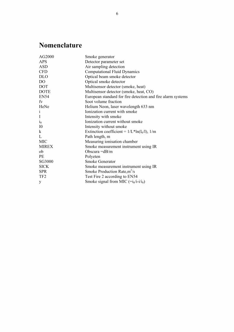
Data on smoke production from smouldering fires is scarce. Tewardson4 Mulholland7 and Drysdale8 have collected some data. Tewardson4 reports that the smoke production, going from flaming to non-flaming combustion, increases a factor of 10 for Red Oak while the difference for Polyurethane is only a factor of 1.7. The ratio obtained here in this work is 4.5 for the PE-box and 0.8 for the white single conductor used in test Cable2 and Cable3. Tewardson reports a Mass Optical density of smoke for Non flaming combustion of Red Oak of 0.3 m2/g (= 3 obm3/g) while Drysdale reports a smoke potential of about 1.8 obm3/g (=0.18 m2/g) for Non Flaming Fibre Insulation Board, Birch plywood, Chipboard and Hardboard. The values obtained here are 4.2 obm3/g for the TF2 fires and 0.4 obm3/g for the particleboard; the particleboard was, however, ignited. Drysdale reports a smoke potential of 1.8 obm3/g for PVC while Mulholland reports 1.2-6.4 depending on the PVC. One can expect that the "Extra plug hole" and some of the cables tested in this project were made of PVC; this gives possible values in the range 0.4 - 8.7 obm3/g for PVC in this project. Due to the large diameter of the MIREX beam (i.e. 4 cm) it was not possible to mount the MIREX close to the smoke measurement position in the cone calorimeter. Instead the MIREX was mounted in a larger duct after the main cone calorimeter duct. Therefore one cannot compare the extinction coefficient obtained by the MIREX and the HeNe laser directly. Instead one has to compare the Smoke Production Rate, SPR. SPR is calculated as the extinction coefficient k times the volumetric flow. A comparison is made between

12

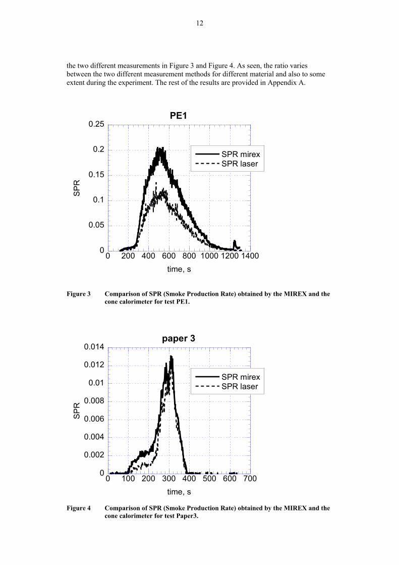
the two different measurements in Figure 3 and Figure 4. As seen, the ratio varies between the two different measurement methods for different material and also to some extent during the experiment. The rest of the results are provided in Appendix A.

0

0.05

0.1

0.15

0.2

0.25

0 200 400 600 800 1000 1200 1400

PE1

SPR mirexSPR laser

SP

R

time, s

Figure 3 Comparison of SPR (Smoke Production Rate) obtained by the MIREX and the

cone calorimeter for test PE1.

0

0.002

0.004

0.006

0.008

0.01

0.012

0.014

0 100 200 300 400 500 600 700

paper 3

SPR mirexSPR laser

SP

R

time, s

Figure 4 Comparison of SPR (Smoke Production Rate) obtained by the MIREX and the cone calorimeter for test Paper3.

13

Some researchers have studied the smoke density or production measured using different wavelengths, however none of these provide an answer to how the smoke density varies relative to the measuring wavelength. The results from Coppa and La Malfa9 are difficult to interpret since the measurements with the different wavelengths were not performed at the same time. Tewarson4 has reported single values for smoke production measured at three different wavelengths, however the results from Andersson1 indicate that the ratio between the smoke density measured at the different wavelengths varies during the fire scenario. In this investigation, the SPR measured with the MIREX was higher than the SPR measured with the HeNe laser. According to theory10 and other investigators1,4,9 it should be the other way around. Therefore an additional measurement was performed using a 670 nm diode laser at the MIREX measuring point. This extra measurement indicated that the SPR measured at the MIREX measuring point was higher than at the HeNe-laser measuring point. The uncertainty of this measurement was however high and therefore this measurement is not reported here. Recently the smoke was analysed at the same two measuring points by an impactor, i.e. an instrument that sort out particles by weight in a cyclone. This measurement did not give any indication on that the smoke had aged be-tween the points. The amount of particles found in the MIREX position was less, but the particle size distribution was the same, so the discrepancy between the measurements is still not resolved.

14

3 Smoke Detector sensitivity Smoke detectors are usually tested against the EN54 standard6. According to the standard the detector is tested in 4 different test fires. Data on detectors performance against other fires is, however, not publicly available. In this project different types of detectors were tested in an EN54 room (10 m long, 6 m wide and 4 m high) against some of the fires tested in the cone calorimeter and against a SG3000 smoke generator. The detectors tested were supplied and mounted by Siemens Fire Safety in the ceiling according to the EN54 standard. The detectors were mounted in the ceiling along a circle with the centre above the fire. The MIC and the detectors were placed on a 3 m radius from the fire. The distance between each detector was 20 cm and the distance between the MIC and detector 1 and 2 was 30 cm. The SICK was placed 3.35 m from the centre. The beam detector was placed 2.5 m from the centre of the room with 8 m between detector and reflector. The placement of the detectors is indicated in Figure 5. The detectors and sensitivity settings used are listed in Table 2. In all 17 tests were performed as listed in Table 3. The sensitivities and types of the detectors were chosen to represent typical sensitive detectors used in industries today.

fire location

86

42

75

31

MIC

samplingsystem

lase

rSI

CK

line

dect

ecto

r

refle

ctor

10m

6m

Figure 5 Placement of detectors in the EN54 room at Delta Electronics.

Table 2 Detectors used for the tests.

Position (in Figure

5)

Detector and setting Nominal aerosol density at alarm (EN54-7 smoke tunnel test)

Meets EN54-7

Comments

1 DOT1151A, APS007 m = 3 %/m Yes Multisensor detector, optical smoke and heat.

2 DOT1151A, APS006 m = 6 %/m Yes Multisensor detector, optical smoke and heat.

3 DO1151A, APS006 m = 3 %/m Yes Optical smoke detector

15

Position (in Figure

5)

Detector and setting Nominal aerosol density at alarm (EN54-7 smoke tunnel test)

Meets EN54-7

Comments

4 DO1151A, APS005 m = 3 %/m Yes Optical smoke detector (slower signal evalua-tion than APS006)

5 DO1151A, APS007 m = 1.5 %/m Yes Optical smoke detector 6 F910, Sens 1 (-), small

smoke entry, short integration)

y = 1.3 Yes Ionisation smoke detector

7 DO1153A, APS072SH m = 0.5 %/m Optical detector, normal use in air sampling systems

8 F910, Sens 2, big smoke entry, short integration

y = 0.9 Yes Ionisation smoke detector

Beam DLO1191, alarm at 50% obscuration

Optical beam detector operated at a medium sensitivity

Sampling DO1161A (in a Titanus 3000, setting for full scale 0.25%/m and normal mode operation)

m = 0.25 %/m (at full scale)

The three different alarm levels are at 33, 66 and 100% of full scale.

Table 3 Tests performed in the EN54 room

Filename Fire Comments SG30001 Smoke generator SG3000 SG30002 Smoke generator SG3000 SG30003 Smoke generator SG3000 Detector6 and 8 were not reset before start

of test SG30004 Smoke generator SG3000 Paper1 Corrugated cardboard in portable cone,

12 kW/m² Flashed at end

Paper2 Corrugated cardboard in portable cone, 12 kW/m²

No CO/CO2 measurement

Paper3 2 pieces of corrugated cardboard, 12 kW/m²

Gren1 Extra plug hole in cone, 20 kW/m² Gren2 Extra plug hole in cone, 20 kW/m², but

distance between material and cone changed so therefore the radiation is higher

Radiation start 20 s after measurement start

Cotton TF3 Paper4 Corrugated cardboard in portable cone,

20 kW/m², two pieces of paper Exposure started 14 s after measuring started. Did not ignite. Probably problem with CO/CO2 measurement

PE1 Blue PE-box 20 kW/m² Exposure started 21 s after measurement started, some measurements were started after the radiation

PE2 Blue PE-box 20 kW/m² Exposure started 17 s after measurement started. Probably problem with CO/CO2 measurement. Steady burning after 2 min.

PE3 Blue PE-box 20 kW/m² Exposure started 18 s after measurement started. Probably problem with CO/CO2 measurement

16

Filename Fire Comments Paper5 Corrugated Cardboard, 3 pieces.

20 kW/m² plus match Fire started 30 s after measuring started.

TF2a TF2 No CO/CO2 measurement TF2b TF2 Probably problem with CO/CO2

measurement The time to alarm is presented in Table 4. Empty places means that no alarm was regis-tered during the experiment. For the sampling detector level 3 was used for alarm. Time to alarm is also presented in Figure 6. If one puts an order number in each experiment where the detector that first gave alarm gets number one and sum up all the order number except for test SG3003, since the ionisation detectors were not reset before that test, we get an ordering like; sampling, detector7, beam, detector5, detector3, detector1, detector8, detector2, detector4 and detector6. The result is in agreement with the sensitivity results obtained by the EN54-7 test provided in Table 2. Table 4 also indicates that the ionisation detectors are better in detecting the SG3000, the flaming and the paper fires compared to the other fires. The smoke obscuration m, dB/m measured with both SICK and a HeNe laser and the parameter y at the time for alarm are presented in Table 5 - Table 7. The parameter y is calculated as

00

ii

ii

y −=

where i0 is the ionisation current without smoke and i the ionisation current with smoke. Studying Table 5 - Table 7 do not, however, make it possible to make any further conclusions. Table 4 Time to alarm (s) from start of fire.

sampling beam detector7 detector5 detector1 detector3 detector6 detector2 detector4 detector8gren1 123 250 154 198 272 264 288 292 296gren2 221 602 412 542 622 594 1005 700 620 592PE1 161 300 226 296 336 330 360 382 477PE2 201 234 244PE3 216 314 270 326 334 336 388 380 488TF2a 195 200 242 244 248 252 359 272 314 315TF2b 187 180 222 222 224 232 354 234 272 273Paper1 157 174 214 230 Paper2 165 224 Paper3 224 272 242 268 288 282 356 342Paper4 101 96 108 120 114 126 164 118Cotton 92 94 134 146 140 130 167 168 224 144SG3001 55 54 56 60 58 52 73 94 108 59SG3002 64 54 62 66 64 60 69 68 112 52

SG3003 65 18 54 52 56 54Not in operation 68 100

Not in operation

SG3004 62 76 58 60 68 66 83 84 108 39

17

gren

1gr

en2

PE

1P

E2

PE

3TF

2aTF

2bP

aper

1P

aper

2P

aper

3P

aper

4co

tton

SG

3001

SG

3002

SG

3003

SG

3004

0

200

400

600

800

1000

1200

time to alarm, s

samplingdetector7beamdetector5detector3detector1detector8detector2detector4detector6

Figure 6 Time to alarm for the different tests and detectors. For the sampling system

level three was used as time to alarm. When no alarm was registered no bar is shown for that case.

Table 5 Ionisation current y at time of alarm.

sampling beam detector7 detector5 detector1 detector3 detector6 detector2 detector4 detector8

gren1 0.14 0.5 0.21 0.33 0.64 0.64 0.67 0.67 0.69 gren2 0.1 0.76 0.37 0.67 0.88 0.7 1 0.79 0.88 0.7 PE1 0.15 0.28 0.26 .28 .37 .42 .5 .52 .73 PE2 0.4 0.58 0.67 PE3 0.17 0.28 0.19 0.35 0.37 0.4 0.42 0.42 0.67 TF2a 0.02 0.02 0.1 0.1 0.1 0.15 1.5 0.69 1.1 1.1 TF2b 0.06 0.06 0.23 0.23 0.26 0.35 1.6 0.42 0.7 0.7 Paper1 0.06 0.06 0.28 0.33 Paper2 0.05 0.19 Paper3 0.02 0.3 0.02 0.2 0.26 0.23 0.67 0.67 Paper4 0.5 0.37 0.79 0.82 0.96 0.64 0.82 0.88 Cotton 1.1 1.1 1.5 2 1.9 1.2 2 2.1 1.8 2 SG3001 1.1 1.1 1 1 1 1.2 1.6 2.7 2.3 1 SG3002 1.6 1.4 1.5 1.7 1.6 1.6 1.7 1.7 2.4 1

SG3003 1.9 0 1.6 1.2 1.6 1.6 Not in operation 1.9 2.1

Not in operation

SG3004 1.6 1.6 1.8 1.6 1.5 1.5 1.7 1.8 2.1 1

18

Table 6 Smoke obscuration m (dB/m) at time of alarm measured with SICK.

sampling beam detector7 detector5 detector1 detector3 detector6 detector2 detector4 detector8gren1 0.05 0.225 0.05 0.1 0.425 0.375 0.525 0.5 0.625 gren2 0.025 0.2 0.05 0.125 0.25 0.2 1.225 0.35 0.25 0.2 PE1 0 0.15 0.05 0.15 0.4 0.35 0.525 0.75 1.05 PE2 0.075 0.15 0.15 PE3 0.05 0.125 0.05 0.2 0.3 0.275 0.45 0.5 1 TF2a 0.225 0.25 0.575 0.625 0.675 0.775 2.07 1.27 1.77 1.8 TF2b 0.2 0.2 0.72 0.72 0.75 0.8 2.1 0.8 1.4 1.4 Paper1 0.02 0.06 0.15 0.1 Paper2 0.025 0.075 Paper3 0.025 0.15 0.05 0.175 0.2 0.175 0.125 0.2 Paper4 0.15 0.15 0.175 0.175 0.225 0.175 0.1 0.225 Cotton 0.175 0.175 0.275 0.3 0.3 0.225 0.5 0.5 0.475 0.3 SG3001 0.2 0.2 0.2 0.15 0.2 0.2 0.175 0.325 0.325 0.15 SG3002 0.225 0.2 0.25 0.2 0.225 0.275 0.25 0.225 0.325 0.2

SG3003 0.25 0.025 0.2 0.125 0.225 0.2 Not in operation 0.225 0.5

Not in operation

SG3004 0.25 0.25 0.2 0.275 0.25 0.25 0.3 0.3 0.35 0.15 Table 7 Smoke obscuration m (dB/m) measured with HeNe laser at time of alarm.

sampling line detector7 detector5 detector1 detector3 detector6 detector2 detector4 detector8gren1 0.019 0.28 0.04 0.12 0.4 0.39 0.59 0.53 0.57 gren2 .0004 0.24 0.039 0.13 0.31 0.18 1.53 0.51 0.31 0.18 PE1 0.016 0.41 0.076 0.44 0.5 0.54 0.77 0.89 1.07 PE2 0.08 0.18 0.23 PE3 0.05 0.18 0.077 0.3 0.24 0.27 0.71 0.56 1.04 TF2a 0.22 0.31 0.65 0.6 0.91 1.1 3.1 1.38 2.3 2.3 TF2b 0.25 0.26 1 1 1.1 1.1 2.7 1.4 2.1 2 Paper1 0.026 0.076 0.17 0.176 Paper2 0.013 0.087 Paper3 0.05 0.37 0.076 0.49 0.36 0.36 0.21 0.32 Paper4 0.2 0.16 0.31 0.36 0.31 0.32 0.151 0.36 Cotton 0.36 0.38 0.81 0.66 0.59 0.85 1.01 0.96 1.02 0.67 SG3001 0.35 0.35 0.49 0.37 0.45 0.28 0.7 0.61 0.39 0.39 SG3002 0.45 0.4 0.48 0.41 0.45 0.5 0.36 0.38 0.36 0.36

SG3003 0.43 0 0.42 0.51 0.49 0.42 Not in operation 0.5 0.83

Not in operation

SG3004 0.36 0.39 0.52 0.41 0.53 0.5 0.66 0.63 0.61 0.2 The smoke density was measured during the test using a diode laser with a wavelength of 670 nm and the SICK which uses an IR wavelength (the same as MIREX), a comparison between the two different measuring methods is presented in Figure 7 - Figure 8. In addi-tion the CO and CO2 concentration was measured during the test together with the tem-perature. However, no significant CO concentration was detected during the tests, this was probably mainly due to problems with the CO/CO2 analyser.

19

m, dB/m

0

0.5

1

1.5

2

2.5

3

0.0 60.0 120.0 180.0 240.0 300.0 360.0 420.0 480.0

time, s

laser mm, SICK

Figure 7 Smoke obscuration measured using a diode laser and the SICK for test

SG3001.

m, dB/m

0

0.2

0.4

0.6

0.8

1

1.2

1.4

0.0 300.0 600.0 900.0 1200.0

time, s

laser mm, SICK

Figure 8 Smoke obscuration measured using a diode laser and the SICK for test PE1.

As seen in Figure 7 and Figure 8, the laser obscuration is higher than the SICK obscura-tion, which complies better with theory. It is also clearly seen that the ratio between the two measurements differs for different fuels. The rest of the results are provided in Appendix A.

20

4 Ventilation systems The ventilation systems used in industries can be divided into two main different types, i.e. mixing systems, which is a "well stirred reactor" type of system where the tempera-ture is the same in the whole room, and displacement systems, where a temperature gra-dient is maintained in the room with high temperatures close to the ceiling, i.e. cold air is supplied at floor level and warm air is extracted higher up. The velocities close to the air supplies can be substantial in the former case while the temperature gradient causes problem in the latter case. It is also common with mixtures of the two different types of ventilation in a room. In many cases there is also a dead volume close to the ceiling that does not take part in the ventilation flow. For ventilation purposes it is the climate rather close to the floor where people are present that is interesting. Ventilation designers do not care about what happens closer to the ceiling. This makes it difficult to get data on the temperature etc. close to the ceiling without measuring at the site.

21

5 Pre-experimental CFD simulations Some CFD simulations were made before the full-scale experiments, these are discussed below. 5.1 The EN54 room A first attempt was made to simulate the results from the EN54 room tests with the PE-box3. This was made mainly to familiarise with the conserved scalar technique and not much effort was spent on modelling correctly the fire source. The work continued, how-ever, in the second project with more thorough simulations presented below. In order to be able to simulate the smoke source as accurate as possible the velocity and temperature above the source was measured11. These results were then compared with the results from different ways of representing the smoke source. These comparisons are provided in Figure 9 and Figure 10. It was decided to use case g since this seemed to be the closest to the experimental values. The legend refers to: the area of the source (8cm x 8cm), the inlet velocity of the smoke and hot air (0.25 m/s), the simulation was made over the entire room since an inter-polation error occurred on the mirror boundaries if only one quarter of the room was simulated (in the whole room) and the Prandtl number for the enthalpy was increased by 10% (Prandtl number +10% for enthalpy).

290300310320330340350360370380390400410420430440

0 0.2 0.4 0.6 0.8 1 1.2 1.4 1.6

height (m)

tem

pera

ture

(K)

a - 12cmx12cm; 723K; 0.15m/s

b - 8cmx8cm; 723K; 0.15m/s

c - 8cmx8cm; 723K; 0.25m/s

d - 8cmx8cm; 723K; 0.25m/s in the whole room

e - 8cmx8cm; 823K; 0.25m/s

f - laminar model; 723K; 0.15m/s

g - 8cmx8cm; 773K; 0.25m/s in the whole room; prandtlnumber +10% for enthalpyexperiments

Figure 9 Temperature profile above the smoke source.

22

0

0.1

0.20.3

0.4

0.5

0.6

0.70.8

0.9

1

1.1

1.21.3

1.4

1.5

0 0.2 0.4 0.6 0.8 1 1.2 1.4height (m)

Velo

city

(m/s

)

a - 12cmx12cm; 723K; 0.15m/s

b - 8cmx8cm; 723K; 0.15m/s

c - 8cmx8cm; 723K; 0.25m/s

d - 8cmx8cm; 723K; 0.25m/s in the whole room

e - 8cmx8cm; 823K; 0.25m/s

f - laminar model; 723K; 0.15m/s

g - 8cmx8cm; 773K; 0.25m/s in the whole room; prandtl number+10% for enthalpyexperiments

Figure 10 Velocity profile above the smoke source

The smoke source was used together with a 0.5 respectively 1 °C/m temperature gradient in the EN54 room. The result for the 1 °C/m case after 1 minute is presented in Figure 11. As seen the smoke reaches the ceiling despite the temperature gradient.

Figure 11 Smoke profile in the 1°C/m case after 1 minute.

5.2 Temperature gradient in a large room The same smoke source was used in a large room 10 m high with a temperature gradient of 0.5 respectively 1 °C/m. The results from the simulations at time 10 minutes are pre-sented in Figure 12 and Figure 13. From these figures we see that the smoke stops at a certain height, in the 0.5°C/m case at about 5 m and in the 1°C/m at about 4 m above the floor.

23

Figure 12 Smoke profile after 10 minutes in the 0.5 °C/m case.

Figure 13 Smoke profile after 10 minutes in the 1 °C/m case.

After discussions with Phil Rubini who has written most of the CFD code SOFIE ( used for the simulations) it was decided to run the scenario again with the smoke source repre-sented as a volumetric source. The results for the 0.5 °C/m and 1 °C/m case are presented in Figure 14 and Figure 15. As seen the smoke levels stop at about the same height but the profile is not as thick as in the previous case.

4.75 m6.35 m

3.75 m 5 m

24

Figure 14 Smoke field for the volumetric source case after 5 minutes. Temperature

gradient of 0.5°C/m, results in that the smoke levels out at 5 m.

Figure 15 Smoke field after 5 minutes for the volumetric source and a temperature

gradient of 1°C/m. The smoke levels out at 3.9 m. This should be compared with the 3.75 m in Figure 13.

When using the volumetric source a volumetric enthalpy source has to be specified in order to create the buoyancy. This enthalpy source was determined by trial and error, i.e. a source was specified and then the velocity and temperature profiles above the source were compared with the experimentally measured profiles. In the end it turned out that a enthalpy source of 290 W reflected best the experimentally measured profiles. 290 W is a small fire, a light bulb is normally 60 W, and a cooking plate on a household stove produces normally 1000 – 1500 W.

25

5.3 Ventilation system In addition a 12 m high room 165x 200m was simulated. Air was let in with 178 litres/s into the room through 68 air inlets with a diameter of 25 cm placed 10.3 m above the floor11. The air outflow of 12 500 litres/s was in one corner of the building. In order to run the simulation in a reasonable time only one quarter of the room was simulated with only a fourth of the air outflow velocity but the same outflow area. The circular inflows were approximated as 22 cm wide squares. Two different scenarios were simulated, one with the smoke source placed between the inflows and one with the smoke source just under an air inlet. The simulated room geometries are presented in Figure 16 and Figure 17.

Figure 16 Schematic of the ventilation system room in the first case with the smoke source

in between the air inlets.

16 m 8 m

24 m

22.5 m

Outflow

Inflow

Smoke source

26

Figure 17 Schematic of the ventilation system room for the second case where the smoke

source is placed right under an air inlet.

The results from the simulations are presented in Figure 18 and Figure 19. Figure 18 shows the smoke field after 10 minutes in the case when the smoke source is placed in between the air inlets (as described in Figure 16). Figure 19 shows the results after 15 minutes when the smoke source is placed under an air inlet. As seen the smoke will reach the ceiling in both cases, but in the case where the smoke source is placed right under the air inlet the smoke will be delayed and diluted.

Figure 18 The smoke field after 10 minutes when the smoke source is placed in

between the air inlets.

48 m

12 m

32 m

24 m16 m

Smoke source

Outflow

Inflow

27

Figure 19 The smoke field after 15 minutes when the smoke source is placed just under an

air inlet. The smoke source is placed on the right hand side in the figure where the smoke emerges from the floor level.

The ventilation system was also simulated using the other approach with a volumetric smoke source. The smoke field after 10 minutes when the smoke source is placed in between the air inlets is displayed in Figure 20. Comparing with Figure 18 shows that the field looks very similar.

Figure 20 Smoke field after 10 minutes same scenario as in Figure 18 but this time using

the volumetric source.

28

6 Full scale experiments Full-scale experiments were conducted in two different industrial buildings. One series was conducted at Fläkt woods in Enköping and one at IKEA in Jönköping. In both cases the experiments were performed during normal operation of the facility i.e. normal working activities were going on. It means that the experiments were not controlled, for instance gates were opened and closed, machines started and switched off, forklifts were driving around etc. 6.1 Displacement system – Fläkt Woods Fläkt Woods has a displacement ventilation system i.e. a temperature gradient is main-tained in the building. The temperature gradient was measured during the experiments. An example of the outcome of these measurements is provided in Figure 22. The air velocity in the room was measured to be between 0.1 and 0.2 m/s, however close to the air inlets the velocity was somewhat higher. The room is 171 x 90 m with a room height of 7.25 m. During the tests the smoke concentration was measured at three different places with laser diodes with a wavelength of 670 nm. 13 optical point detectors (APS006) and one sampling system (ASD using a DO1153 with parameter set APS071, alarm at 0.25%/m) were mounted as well. Two computers registered the output from these. The results are presented in appendix B. Three different smoke generators were used; these were the TF2 fire according to EN54-7, the SG3000 and one called AG2000 that is under development by Siemens Fire Safety. The tests performed are listed in Table 9. A schematic of the equipment placement is given in Figure 21.

ASD

Det5, Det6

ASD, laser2

Det11, Det12

ASD, laser3

ASD

Det3, Det4

origin

Det1, Det2, Fire, Laser1,

thermocouples

Det7, Det8, Det14 Det9, Det10

Figure 21 Schematic of Equipment placement.

A more precise equipment placement is given in Table 8 using a coordinate system with an origin of coordinates placed at the nearest beam outside all the test equipment at floor level close to the wall.

29

Table 8 Detector placement in the Fläkt Woods tests.

Detector/instrument Coordinates Comments Detector 1 (6.2, 6, 7.1) Detector 2 (6.2, 6, 6.2) Laser 1 (7.4, 5.7, 4.8) Midpoint of measuring

beam Thermocouples (6.7, 5.35, 2.2-7.2) One thermocouple every

half meter Detector 3 (2.25, 6, 7.1) Detector 4 (2.25, 6, 6.2) Detector 5 (6.2, 12.4, 7.1) Detector 6 (6.2, 12.4, 6.2) Laser 2 (6.3, 10.7, 6.25) Midpoint of measuring

beam Detector 7 (11.25, 6, 7.1) Detector 8 (11.25, 6, 6.2) Detector14 (11.25, 6, 4.7) Detector 9 (15.75, 6, 7.1) Detector 10 (15.75, 6, 6.2) Detector 11 (11.25, 12.4, 7.1) Detector 12 (11.25, 12.4, 6.2) Laser 3 (10.8, 10.7, 6.25) Midpoint of measuring

beam ASD (2.25-11.25, 10.7, 6.4) One sampling point close to

each detector pair in the x-direction

Table 9 The tests conducted at Fläkt Woods

Test Fire Coordinate Comments 1 SG3000 (7,6,0) Problems with detector signals 1-6 2 SG3000 (7,6,0) 3 AG2000 Disco Fluid 2.2 kW (7,6,0) 4 TF2 20 old type wooden

sticks (7,6,0) Interrupted due to loss of power

5 TF2 20 old type wooden sticks

(7,6,0) Interrupted due to loss of power


(7,6,0) Interrupted when starts to flame

7 SG3000 (7,6,0) 8 AG2000 Paraffin oil (7,6,0) Very little smoke was produced 9 AG2000 Disco Fluid (7,6,0) Interrupted ignition of paraffin oil 10 AG2000 Disco Fluid 4.6 kW (7,6,0) 3-4 drops per second, the liquid lasted

6 min 15 s 11 AG2000 70 g PE box 2.2 kW (7,6,0) Increased to 4.6 kW at 18 minutes 12 AG2000 24 TF2 sticks 2.2

kW (7,6,0)


(8,6,0) Interrupted when flaming

30

Temperature, °C

22.523

23.524

24.525

25.526

26.5

0.00 200.00 400.00 600.00

time, s

7.2 m degC6.7 m degC6.2 m degC5.7 m degC5.2 m degC4.7 m degC4.2 m degC3.7 m degC3.2 m degC2.7 m degC2.2 m degC

Figure 22 The temperature gradient at the Enköping tests.

Studying the results in Appendix B the following observations can be made:

• The smoke concentration measured with the lasers and detectors are in reasonable agreement with each other.

• The sampling system gave alarm first followed by the detectors close to the fire i.e. detector 1 and 2.

• Detectors 9, 10, 11 and 12 gave usually alarm after detector 1 and 2. This is a bit strange since the air movement in the building, according to the ventilation staff at the site, ought to be more towards detector 3 and 4. On the other hand, this was a question that caused a lot of discussion and after discussion with other ventila-tion consultants they concluded that the air should not drift in any direction.

• There was a slight tendency that the lower detectors i.e. detectors with even numbers gave alarm and warning before the detectors close to the ceiling i.e. detectors with odd numbers. However, for time to pre-alarm it was the other way around.

• The TF2 fire was difficult to detect. In test 6 only warnings were achieved. In test 13 the fire was moved about 1 m towards detector 7 and 8. In this test the smoke took another route compared to the other tests, i.e. in this test the smoke took the route that was first predicted by the ventilation staff. The smoke kept hanging in the air and moved downwards to the people working in the building.

• Comparing test 3 (AG2000 2.2 kW) and test 10 (AG2000 4.6 kW) shows that a higher heat results in better possibility to detect the fire. This is partly due to that the smoke production increases with the applied heat in the AG2000 but still there is a tendency for the smoke to reach higher if the heat applied increases.

• There was a problem that the smoke from the disco fluid used for the AG2000 did not have long lifetime enough in such a big building. Using the wooden sticks and especially the PE box worked better.

The fact that the smoke took a different route in test 13 is probably not so much due to that the fire was moved 1 meter to the side in this case. The smoke took a slightly different route also in test 1. This is probably caused by changes in the airflow pattern due to gates being opened etc. Before the test series started all air inlets were reset to the air-flow they were planned to have according to the ventilation staff. Walking around the

31

second day showed however that the production staff had changed the ventilation by means of e.g. corrugated cardboard to eliminate draught at their workplaces. 6.2 Mixing system – IKEA The experiments were conducted in a room 165 x 200 m. The ceiling height was 11.8 m. The building has a total mixing ventilation system. The temperature gradient in the room was measured during the tests together with the air velocity below one of the inlets. The smoke concentration was measured at three different places with laser diodes with a wavelength of 670 nm. 12 optical point detectors (DO1151/APS006), four CO/optical detectors (DOTE/APS216), four beam detectors, a video and one sampling system (ASD) were mounted as well. APS006 means that the detector gives alarm at 3 %/m provided that the 60s pre-history shows a not negligible smoke signal that is mainly increasing. Danger level 1 and 2 is reached at 1 respectively 2 %/m. The APS216 means that the detector when exposed to only aerosols gives alarm at 3%/m like the DO-detectors. When the detector is exposed to a rising CO-concentration (in single digit ppm range) then the smoke sensitivity is increased to 1.5 %/m. Table 10 Detectors and measuring instruments placement

Detector/instrument Coordinates comments Detector 1 (5.35, 0, 11.3) DO1, optical detector Detector 2 (5.35, 0, 9.75) Detector 3 (5.35, 6.1, 11.3) Detector 4 (5.35, 6.1, 9.75) Detector 5 (5.35, 12.2, 11.3) Detector 6 (5.35, 12.2, 9.75) Detector 7 (17.5, 12.2, 11.3) Detector 8 (17.5, 12.2, 9.75) Detector 9 (17.5, 6.1, 11.3) Detector 10 (17.5, 6.2, 9.75) Detector 11 (17.5, 0, 11.3) Detector 12 (17.5, 0, 9.75) DOTE 1 (5.35, 6.1, 11.3) Combination of Optical and

CO detector DOTE2 (5.35, 6.1, 9.75) DOTE3 (17.5, 6.1, 11.3) DOTE4 (17.5, 6.2, 9.75) DLO1 (0, 2.0, 5.6) Line of sight 2 x 24.9m DLO2 (0, 2.0, 9.4) Line of sight 2 x 29.8m DLO3 (0, 6.5, 9.4) Line of sight 2 x 29.8m DLO4 (0, 6.5, 5.6) Line of sight 2 x 24.9m Laser1 (5.35, -3, 11.3) Laser2 (17.9, 1.0, 11.3) Laser 3 (7.4, 6.1, 9.75) ASD (0-25, 6.1, 9.75) 6 Holes 4 m between the

holes Velocity (5.35, -4, 9.45-5.45)

32

The point detectors were mounted in pairs, odd numbers close to the ceiling and even numbers 1.5 meter below that. Computers registered the output from all detectors. Three different smoke generators were used, these were the TF2 fire according to EN54, the SG3000 and one called AG-2000 that is under development by Siemens Fire Safety. The fires were placed at different locations. A schematic drawing is given in Figure 23 and the coordinates in Table 10. The coordinates are from a origin placed in the upper left corner of the schematic with the x direction down along the paper, y in the right direction of the paper and z out of the paper. All test results are reported in Appendix C.

Figure 23 Schematic of detector and fire placement.

33

Table 11 Fire tests conducted.

Test Fire Coordinates Comments 1 SG3000 (9.6, 5.5, 0) 2 SG3000 (17.6, 5.9, 0) 3 SG3000 (17.7, -2.6, 0) 4 SG3000 (11.0, -2.4, 0) Corrupt data file from laser 5 TF2 new type of wooden sticks (9.0, 5.5, 0) 6 AG2000 new type wood, 2.2 kW (9.0, 5.5, 0) 7 AG2000 old type wood, 2.2 kW (12.6, 5.3, 0) 8 AG2000 old type wood, 4.6 kW (12.6, 5.3, 0) 9 AG2000 70g PE-box, 4.6 kW (12.6, 5.3, 0) 10 SG3000 (5.35, -4, 4) At roof to measurement room

close to an air inlet. Studying the results in Appendix C the following observations can be made:

• The measured smoke concentrations were rather low in all tests. • The results include straight lines that mean that there was a data error in the trans-

mission from the detector to the computers. • The sampling system gave alarm/warning first. • The detectors closest to the fire gave alarm/warning earlier than the detectors

more far away • There was also a tendency in these tests that the detectors placed 1.5 m below the

ceiling gave higher smoke signals then those placed close to the ceiling. • Looking at test 1 the DOTE signals it seems like DOTE-1 gives signal for CO but

not so much for obscuration and then for DOTE 2 it is the other way around. • In test 7 one sees that the DOTE detectors receive CO but no smoke. • In test 3 the detectors 11 and 12 give less smoke obscuration than the laser 2. • There is also a tendency for CO but no smoke in test 3. • Comparison of the time to warning, pre alarm and alarm for the tests between

DO3 and 4 with DOTE 1 and 2 and DO 9 and 10 with DOTE 3 and 4 indicates that time to warning and pre-alarm is longer for the DOTEs while time to alarm is slightly shorter for the DOTEs. The results from test 8 and 9 are however a bit strange. In this case DOTE 1 gave signal but nothing on DO 3 and 4.

• The beam detectors 1.5 m below the ceiling gave alarm in most tests. • The DLO1 did not give any alarm or warning in any test. • The agreement between the sampling system and the beam detector DLO3 is very

good except for test 7 and 10 where the sampling system shows less obscuration and test 1 where the beam detector signals show a bit less obscuration.

34

7 CFD simulations of the Full scale experiments

The experiments were simulated using the CFD code Sofie. The simulations were based on the simulations in section 5.2 and 5.3 but the dimensions of the rooms and the temperature gradient were changed to the dimensions at the site and the temperature gradient measured during the tests. In addition, the smoke source was changed to the SG3000. Temperature and velocity comparisons between the PE-cone calorimeter and the SG3000 are given in Figure 24 and Figure 25. Figure 26 shows the measured smoke obscuration above the SG3000.

0

20

40

60

80

100

120

140

160

180

200

0 10 20 30 40 50 60 70 80 90 100 110 120 130 140 150height (cm)

tem

pera

ture

smoke generatorPEPE model

Figure 24 Temperature profile for the SG3000 and the PE box from the cone calorimeter.

0

0.2

0.4

0.6

0.8

1

1.2

1.4

1.6

0 10 20 30 40 50 60 70 80 90 100 110 120 130 140 150

height (cm)

velo

city

smoke generatorPEPE model

Figure 25 Velocity profile for the SG3000 and the PE box from the cone calorimeter.

35

m, db/m

0123456789

10

30 90 150 210 270 330 390

time, s

26 cmabovesource65 cmabovesource

Figure 26 Smoke obscuration measured at different heights above the SG3000. The cyclic

behaviour of the SG3000 is clearly seen. No difference between different heights can be observed, which means that the measuring laser covers the entire plume at the different heights.

7.1 Simulation of the test at Fläkt Woods The tests using the SG3000 were simulated, i.e. test 1, test 2 and test 7. These were simulated in a 20 m wide and 15 m deep room. The room height is 7.3 m. The simulation was run using 311 000 cells, the largest cell size was 0.3 x 0.3 x 0.2 m3. The smoke was let in as a conserved scalar through a hole 0.2 m squared with a velocity of 1.5 m/s and a temperature of 340 K in two cases; one case using the normal k-ε model and one case using the modified k-ε suggested by Bill and Nam12. The smoke source was set to 10 dB/m up to time 10 seconds. At time 10 seconds it was assumed to increase linearly with a factor of 7/350 starting at 0.1. In addition, a third simulation where the SG3000 was modelled as a volumetric source was run. In this case the source was 0.2 by 0.2 m in area and 0.1 m high. The enthalpy source was 400 000 W/m3 which results in a total heat release of 1600 W. The smoke source was set to 10 g/s for the first 10 seconds and then increasing linearly from 0.1 g/s up with a factor of 7/350 g/s. The results for all three simulations are presented in Figure 27 - Figure 41.

36

Figure 27 The iso-curve for 1%/m seen from the staircase looking into the building after 6

minutes using the normal k-ε model. The smoke is slowed down by the beam but reaches the ceiling.

Figure 28 The 1%/m isocurve seen from the reception after 6 minutes using the normal k-

ε model. The smoke is slowed down by the beam but reaches the ceiling.

Figure 29 The 2%/m isocurve seen from the reception.

37

Figure 30 The 2%/m isocurve seen from the staircase.

Figure 31 The 3%/m iso curve seen from the reception at time 6 minutes.

Figure 32 The 3%/m iso curve seen from the staircase at 6 minutes.

38

Figure 33 The iso-curve for 1%/m seen from the staircase looking into the building after 6

minutes using the Bill and Nam k-ε model. The smoke is slowed down by the beam but reaches the ceiling even if the plume is wider in this case.

Figure 34 2%/m seen from the staircase after 6 minutes. The simulation was made using

the Bill and Nam turbulence coefficients; the source had a velocity of 1.5 m/s and a temperature of 340 K.

Figure 35 3%/m seen from the staircase after 6 minutes. The simulation was made using

the Bill and Nam turbulence coefficients; the source had a velocity of 1.5 m/s and a temperature of 340 K.

39

Figure 36 1 %/m for the volumetric source seen from the staircase after 6 minutes.

Figure 37 2 %/m for the volumetric source simulation after 6 minutes seen from the stair-

case.

Figure 38 3 %/m for the volumetric source simulation after 6 minutes seen from the stair-

case.

40

Figure 39 1%/m seen from the reception for the volumetric source after 6 minutes.



Determining the source parameters, i.e. area, height and enthalpy source, is a very tedious process for the volumetric source. One has to run the simulation until it has stabilised in order to find out what velocity and temperature profile that results from the source. In

41

addition, the measured smoke obscuration has to be transformed into a soot mass source. The soot mass source rate sm& (kg/s) can be calculated from

LDVm T

s ⋅⋅=

19000&

&

where TV& is the volumetric flow rate in the plume, D is the optical density (ob) and L is the path length (m) over which the optical density is measured. The constant 19000 is the Particulate optical density for smouldering combustion, 19000 ob m3/kg. The simulated soot volume fraction fv is transformed to %/m from

−⋅=⋅⋅⋅

100//%11log101800109.1 4

mfv

where 1800 kg/m3 is the soot density. A comparison between the different simulations and the experiments is made in Table 12. Table 12 Comparing the simulated and measured obscuration, %/m.

Detector/laser Simulation

Simulation Nam and Bill

Volumetric source

Test1 Test2 Test7

Detector1 6.7 5.8 1.8 6 0 Detector2 5.6 5.2 1.4 3.6 0 Detector 3 4.0 3.4 0.9 0.2 0 Detector4 1.6 1.4 0.5 0.2 0 Detector5 2.8 2.4 0.7 0.7 0 Detector 6 1.0 1.2 0.3 0.5 0 Detector7 4.2 3.6 0.8 0.4 2 0.2 Detector8 1.6 1.7 0.5 0.5 0.1 0.1 Detector 9 3.0 2.1 0.7 1.9 2 1.4 Detector10 1.8 1.4 0.6 3 3 2.8 Detector11 2.7 2.3 0.7 4.2 4.6 0.5 Detector 12 1.4 1.3 0.3 0.1 0.2 1.5 Detector 14 2.7 2.3 0.7 11.4 Laser1 14.3 11.7 2.8 57 56 58 Laser2 1.0 1.3 0.3 4.3 3.2 0.14 Laser3 1.4 1.4 0.3 8.2 1.4 0.088 Studying the table and comparing the three experiments it is obvious that these are very stochastic experiments, a feature that CFD simulations cannot capture. Comparing the laser signals with the simulation is somewhat doubtful since the laser measures over one meter while the simulation values are in a single point taken at the middle of the laser measuring beam. The order of magnitude is about the same in the experiments and simulations except for laser 1 and the volumetric source. The simulations do not, however, capture the variation in smoke levels between the different detector locations. For instance the smoke level at detector 7 and 8 differs significantly from the level at detector 3 and 4 in one of the experiments while it does not in the simulation.

42

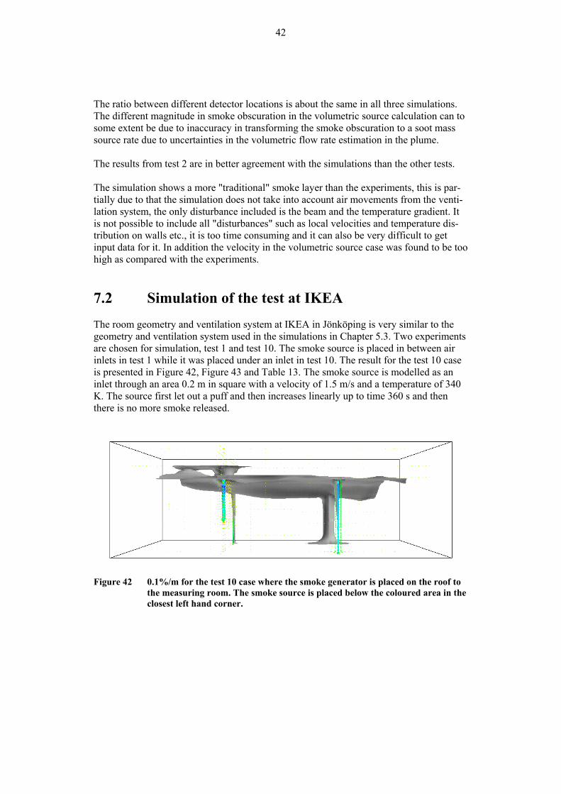
The ratio between different detector locations is about the same in all three simulations. The different magnitude in smoke obscuration in the volumetric source calculation can to some extent be due to inaccuracy in transforming the smoke obscuration to a soot mass source rate due to uncertainties in the volumetric flow rate estimation in the plume. The results from test 2 are in better agreement with the simulations than the other tests. The simulation shows a more "traditional" smoke layer than the experiments, this is par-tially due to that the simulation does not take into account air movements from the venti-lation system, the only disturbance included is the beam and the temperature gradient. It is not possible to include all "disturbances" such as local velocities and temperature dis-tribution on walls etc., it is too time consuming and it can also be very difficult to get input data for it. In addition the velocity in the volumetric source case was found to be too high as compared with the experiments. 7.2 Simulation of the test at IKEA The room geometry and ventilation system at IKEA in Jönköping is very similar to the geometry and ventilation system used in the simulations in Chapter 5.3. Two experiments are chosen for simulation, test 1 and test 10. The smoke source is placed in between air inlets in test 1 while it was placed under an inlet in test 10. The result for the test 10 case is presented in Figure 42, Figure 43 and Table 13. The smoke source is modelled as an inlet through an area 0.2 m in square with a velocity of 1.5 m/s and a temperature of 340 K. The source first let out a puff and then increases linearly up to time 360 s and then there is no more smoke released.

Figure 42 0.1%/m for the test 10 case where the smoke generator is placed on the roof to

the measuring room. The smoke source is placed below the coloured area in the closest left hand corner.

43

Figure 43 0.2%/m for the test 10 case where the smoke generator is placed on the roof to

the measuring room. The smoke source is placed below the coloured area in the closest left hand corner.

Table 13 Simulation and test result for the case Test10, %/m.

Detector/laser Simulation 360 s

Simulation 600 s

Test10 360 s Test10 600s

Detector1 1.1 0.15 0.05 0 Detector2 0.15 0.06 0.02 0.7 Detector 3 0.9 0.2 0.02 0 Detector4 0.002 0.1 0.05 0.3 Detector5 0.6 0.3 0 0 Detector 6 0.004 0.15 0.02 0.02 Detector7 0.5 0.3 0 0 Detector8 0.004 0.1 0.02 0.02 Detector 9 0.7 0.3 0.1 0.02 Detector10 0.002 0.04 0.04 0.1 Detector11 0.007 0.3 0.1 0.04 Detector 12 0.02 0.05 0.04 0.04 DOTE1 0.9 0.2 0 0.05 DOTE2 0.002 0.1 0.02 0.2 DOTE3 0.7 0.3 0.02 0.04 DOTE4 0.002 0.4 0.06 0.06 DLO1 0.00008 0.009 0.007 0.01 DLO2 0.003 0.04 0.15 0.35 DLO3 0.0005 0.04 0.2 0.4 DLO4 0.00008 0.007 0.02 0.02 Laser1 21 0.20 0.4 0.5 Laser2 6.5 3.4 0.07 0.07 Laser3 0.002 0.08 0.6 0.9 ASD 0.001 0.06 0.02 0.2 The results for the test1 case is presented in Figure 44, Figure 45 and Table 14. The smoke source is modelled as an inlet through an area 0.2 m in square with a velocity of 1.5 m/s and a temperature of 340 K. The source first lets out a puff and then increases linearly up to time 360 s.

44

Figure 44 0.1 %/m for the test1 case seen from the measuring room towards the

workshop.

Figure 45 0.2 %/m for the test1 case seen from the measuring room towards the workshop.

Comparing the simulated values with the values from the beam detectors and the sam-pling system is difficult. The value reported for the simulations in Table 13 is the value at the mid point of the beam or sampling system while the experimental values are average values over the entire measuring area for each detector. The experiments show more smoke a bit below the ceiling (i.e. detectors with even numbers) than close to the ceiling. This is, however, not observed in the simulations. Apart from this it is difficult to draw any conclusions except that the simulations do not reflect the experiment reasonably. The geometry used in the simulations was simplified in comparison with the reality, for instance the measuring room and the workshop are not included.

45

Table 14 Comparison between simulated and experimental values for test1 at IKEA.

Detector/laser Simulation (%/m) 360 s Test1 360 s Detector1 8.6 0.014 Detector2 0.3 1.1 Detector 3 9.0 0.69 Detector4 0.22 0.73 Detector5 8.6 0.038 Detector 6 0.097 0.042 Detector7 8.0 0 Detector8 0.0081 1.38 Detector 9 7.1 0.19 Detector10 0.0046 1.14 Detector11 7.1 0.035 Detector 12 0.015 0.018 DOTE1 9 0.21 DOTE2 0.22 0.53 DOTE3 7.1 0.094 DOTE4 0.0046 0.094 DLO1 0.00048 0.00021 DLO2 0.0014 0.0045 DLO3 0.00044 0.003 DLO4 0.00011 0.00007 Laser1 7.7 0.50 Laser2 7.1 0.39 Laser3 0.055 0.76 ASD 0.00025 0.44 7.3 Discussion It is clear that the simulations did not reflect the experiments satisfactorily. There are a number of possible reasons for this. The grid used in the simulations was too coarse. The parametric study indicates, however, that the solutions were grid independent. The grid used for simulating the experiments were similar to the grid used in the parametric study. The time step was too large. The time step used was 1 s in all simulations. The simulation time varied between 2 and 14 days for the different simulations. Decreasing the time step with a factor of 10 would increase the total simulation time a factor of 10. A simulation time longer than several months is hard to justify for such a simplified problem. The scenarios were simplified. In the Fläkt Woods case all machines, air inlets etc. were not put into the simulation as obstructions or heat and air flow producers. The only disturbance included was the temperature gradient. For the IKEA case it was only the air inlet and outlets that were modelled. The workshop and measuring room were not in-cluded. On the other hand, it seems unlikely that the inclusion of the workshop and measuring room would change the results considerably. Of course there can be other sources that produce air currents that we did not identify before and during the experiments.

46

The smoke source was not modelled correctly. The velocity and temperature profile in the centre above the smoke source was measured experimentally and then the smoke source was tuned in to fit these values. This turned, however, out to be very time consuming and difficult. After a couple of weeks it was decided to use the best fit found so far. This process could, maybe, have been improved by measuring the velocity and temperature profile in more points over the smoke source and then representing the smoke source as several small sources with different temperature and velocity. Or, preferably, if there was a function available that automatically determined the best representation of a source with a certain temperature and velocity profile in the plume. The turbulence model used was not appropriate. The k-ε model was used for all simula-tions. In some cases the factors used were those recommended by Nam and Bill12. This did improve the air entrainment in the plume to some extent. Sofie is not useful for such a small fire. The only CFD code used in this project was Sofie. Sofie is developed for use on larger fires than those studied in this project. Perhaps another code more intended to simulate indoor climate or air currents would have been more successful. The problem is not suitable to be solved with CFD. If all other reasons have been investi-gated without any improvement of the result then the only explanation can be that the problem is not suitable to be solved with CFD simulations. It has not been possible to determine what reason(s) is the main explanation for the poor result of the simulations within this project.

47

8 Conclusion The smoke production data presented in this project is consistent with the limited data available on Non-Flaming Combustion in the literature. The experiments performed in the EN54 room showed that the detectors were activated in the order one would expect from the supplier data. The experiments showed also that the ratio between smoke production measured with a laser and the SICK varies between different fuels and burning/vaporisation rate. There are two main different types of ventilation systems used in industries, one is main-taining a temperature gradient in the room, the other uses a total mixing concept. All kinds of mixtures between the two exist as well. Ventilation system manufacturers do not bother about the temperature etc. close to the ceiling, their concern is the climate close to people working and material produced or stored. Therefore "a dead volume", where no air enters, can exist close to the ceiling. It is rather difficult to get data and estimates on airflow patterns etc. for a facility that is in use and have been in use for a while. The systems are changed and new equipment is installed that was originally not planned. In addition, personnel working at the site put up screens etc. in order to prevent themselves from draught etc. The simulations of the full-scale experiments were not very successful. The simulations showed a more traditional smoke layer than the experiments. This is partly due to that the geometry of the room and disturbances was simplified. In the Fläkt Wood case only the temperature gradient and the beam above the fire was modelled while in the IKEA case only the inflows and outflow in the room was modelled. Other geometrical obstructions and airflow patterns within the room were not taken into account. In addition, the turbu-lence model used is known to give to narrow a plume i.e. the air entrainment is under predicted. Adjusting the model by using the constants suggested for fire plumes by Bill and Nam12 did improve the simulations to a limited extent. Furthermore, the difficulties with the simulations can to some extent be due to that the SG3000 differs from a fire and Sofie is mainly intended for simulation of fires. The SG3000 has a higher velocity but lower temperature profile than fires normally have. In addition, one could suspect that the density of the smoke will increase due to coagulation and thus cannot be modelled as a conserved scalar. The parametric study indicates that the temperature gradient required to prevent the smoke from reaching the ceiling in a room 7 m high is substantial. The study was per-formed using a source of 300 W; the SG3000 has a convective heat flow about 5 times that. This implies that other forces than the temperature gradient dilutes the smoke plume as well. These sources include the local air flow pattern due to other heat sources, fork lifts driving by, opening gates, ventilation system etc. especially the beam above the "fire" slowed down the smoke as could be seen in the simulations as well. The full-scale experiments showed that what way the smoke takes differs from each test. Even when all parameters are the same the differences in the smoke field are substantial between each test. This behaviour can never be captured with a CFD simulation. The experiments showed a slight tendency for more smoke at the detectors placed a bit below the ceiling, which indicates that it can be useful to place detector about 10 % from the ceiling (or just below ceiling beams) together with detectors placed in the ceiling. For the IKEA case the experiment showed that the smoke concentration close to the ceiling was lower than the concentration 1.5 m below the ceiling especially after end of

48

smoke from the SG3000. This effect was not seen in the simulations. The reason for this discrepancy could be that the temperature of the ceiling differed from the temperature indoors, but the temperature measurements in the experiments did not indicate such differences, the only test with a temperature difference was test 10, and the difference was only 1º. The fact that the effect was more pronounced after a while could indicate ageing of the smoke. The CFD simulations can be used for studying trends, but for the temperature gradient this can be accomplished by using empirical plume formulas. In order to make true simulations of a facility a huge amount of input data is required and several simulations are required to reflect the different situations that are present during the use of the facility. This makes it probably more efficient to conduct experiments at the site instead. Since CFD simulations visualizes the problem better than empirical formulas for people not so involved in fire problems they can be useful in the construction phase of the building or when planning the detection system at a building not yet built or where it is impossible to conduct full scale experiments. It is very difficult and time consuming to choose the parameters of the smoke inlet so that the velocity and temperature profiles are similar to the experimental profiles. A tool where one could give the profile as input and get the smoke source as output would be useful. SG3000 is useful as a smoke generator since it does not smell and can be used also in sensitive areas. The question is, however, how well the SG3000 reflects a possible small fire. The temperature and velocity profile is not known for small fires, is it more like the profile from the cone or from the SG3000? Another problem is how small fire must be detected. Little work has been done on small fires, probably because it is a difficult problem. Whether a smouldering fire continues to grow or is self extinguished is difficult to predict. Will the fire continue to glow for a long time and then suddenly start to increase or will it start to increase immediately. The glowing fire maybe already has caused severe damage in a sensitive environment when it starts to grow. Finding the optimal placement of detectors is an almost endless project both using simu-lations or experiments since so many different airflow patterns and fires must be covered. The smoke from a larger fire reaches higher than the smoke from a smaller fire. The air-flow pattern depends on the time of the year and day, the activity going on in the build-ing, which machines are in operation, what doors are opened etc. A possible solution is placing sensitive detection at several heights. If point type smoke detectors are used they may have to be so sensitive that they are outside the normal sensitivity range allowed within EN54-7. Using such sensitive detectors requires an intelligent system to minimize false alarms.

49

References 1 Andersson, P. "Evaluation and Mitigation of Industrial Fire Hazards" LUTVDG/(TVBB-

1015) Lund 1997.

2 Thomas, P. H. "The role of the Initial Conditions in the detection of fires" in Minutes from EUSAS-BRANDFORSK WORKSHOP on smoke Detection, September 26-27, 1994, LUTVDG/TVBB 3081, Lund.

3 Andersson, P. and Ingason, H. "Smoke Production and Detection" SP Technical Note 2001:35 Borås 2001

4 Tewardson, A. "Generation of Heat and Chemical Compounds in Fires" in The SFPE Hand-book of Fire Protection Engineering, First ed.1988, pp.1.179-1.199.

5 International Standard – Reaction-to-fire tests -- Heat release, smoke production and mass loss rate -- Part 1: Heat release rate (cone calorimeter method) ISO 5660-1:2002(E). Inter-national Organization for Standardization, Geneva, 2002.

6 EN54-7:2000 E, "Fire Detection and Fire Alarm Systems – Part 7: Smoke detectors – Point detectors using scattered light, transmitted light or ionization".

7 Mulholland, G. "Smoke Production and Properites" in The SFPE Handbook of Fire Protection Engineering, First ed.1988, pp.1.368-1.377.

8 Drysdale D., An Introduction to Fire Dynamics, second edition, John Wiley & Sons, Chichester 1998

9 Coppa, P. and La Malfa A. "Light extincion by Fire Smokes", Journal of Fire Sciences vol.15 no. 3, pp.180-202, 1997.

10 Holmstedt, G., Magnusson, S.E. and Thomas, P.H. "Detector environment and detector response"LUTVDG/(TVBB-3039) Lund 1987.

11 Conte, F. "CFD simulations of smoke detection in rooms with high ceilings" SP Technical Note 2002:30, Borås 2002.

12 Nam, S. and Bill, R. "Numerical Simulation of Thermal Plumes", Fire Safety Journal Vol. 21, No. 3, pp. 231-256, 1993.

A1

Appendix A Smoke production results

1 Cone calorimeter tests The result from the smoke measurements are provided in figure 1- figure 27 below.

0

0.05

0.1

0.15

0.2

0.25

0 200 400 600 800 1000 1200 1400

PE1

SPR mirexSPR laser

SP

R

time, s

Figure 1 Comparison of SPR obtained by the MIREX and the cone calorimeter for test PE1.

0

0.05

0.1

0.15

0.2

0 200 400 600 800 1000 1200 1400

PE2

SPR mirexSPR laser

SP

R

time, s

Figure 2 Comparison of SPR obtained by the MIREX and the cone calorimeter for

test PE2.

A2

0

0.05

0.1

0.15

0.2

0 300 600 900 1200 1500 1800

PE3

SPR mirexSPR laser

SP

R

time, s


0

0.01

0.02

0.03

0.04

0.05

0 300 600 900 1200

PE4

SPR mirexSPR laser

SP

R

time, s


A3

0

0.01

0.02

0.03

0.04

0.05

0.06

0.07

0 120 240 360 480

Paper 1

SPR mirexSPR laser

SP

R

time, s

Figure 5 Comparison of SPR obtained by the MIREX and the cone calorimeter for test Paper1.

0

0.0001

0.0002

0.0003

0.0004

0.0005

0.0006

0.0007

0 120 240 360 480 600 720

Paper 2 SPR mirexSPR laser

SP

R

time, s


A4

0

0.002

0.004

0.006

0.008

0.01

0.012

0.014

0 100 200 300 400 500 600 700

paper 3

SPR mirexSPR laser

SP

R

time, s


0

0.002

0.004

0.006

0.008

0.01

0.012

0 120 240 360 480 600 720

Paper 4

SPR mirexSPR laser

SP

R

time, s


A5

0

0.002

0.004

0.006

0.008

0.01

0.012

0.014

0 120 240 360 480 600 720

Paper 5

SPR mirexSPR laser

SP

R

time, s


0

0.005

0.01

0.015

0.02

0 240 480 720 960 1200

Glim 1

SPR mirexSPR, laser

SP

R

time, s

Figure 10 Comparison of SPR obtained by the MIREX and the cone calorimeter for

test Lighter1.

A6

0

0.0005

0.001

0.0015

0.002

0.0025

0 240 480 720 960 1200

Glim 2

SPR mirexSPR laser

SP

R

time, s

Figure 11 Comparison of SPR obtained by the MIREX and the cone calorimeter for test Lighter2.

0

0.002

0.004

0.006

0.008

0.01

0 120 240 360 480 600 720 840 960

Safe 1

SPR mirexSPR laser

SP

R

time, s

Figure 12 Comparison of SPR obtained by the MIREX and the cone calorimeter for test Safe1.

A7

0

0.002

0.004

0.006

0.008

0.01

0.012

0 240 480 720 960

Glim 3

SPR mirexSPR laser

SP

R

time, s

Figure 13 Comparison of SPR obtained by the MIREX and the cone calorimeter for test Lighter3.

0

0.02

0.04

0.06

0.08

0.1

0 600 1200 1800 2400

Gren 1

SPR mirexSPR laser

SP

R

time, s

Figure 14 Comparison of SPR obtained by the MIREX and the cone calorimeter for test Gren1.

A8

0

0.02

0.04

0.06

0.08

0.1

0 300 600 900 1200 1500 1800

Gren 2

SPR mirexSPR laser

SP

R

time, s


0

0.02

0.04

0.06

0.08

0.1

0 300 600 900 1200 1500

Gren 3

SPR mirexSPR laser

SP

R

time, s


A9

0

0.005

0.01

0.015

0.02

0.025

0.03

0.035

0.04

0 300 600 900 1200 1500

Cable 1

SPR mirexSPR laser

SP

R

time, s

Figure 17 Comparison of SPR obtained by the MIREX and the cone calorimeter for test Cable1.

0

0.005

0.01

0.015

0.02

0.025

0.03

0.035

0 120 240 360 480 600 720

Cable 2

SPR mirexSPR laser

SP

R

time, s


A10

0

0.02

0.04

0.06

0.08

0.1

0.12

0.14

0 120 240 360 480 600

Cable 3

SPR mirexSPR laser

SP

R

time, s


0

0.05

0.1

0.15

0 120 240 360 480 600 720 840

Foam 1

SPR mirexSPR laser

SP

R

time, s

Figure 20 Comparison of SPR obtained by the MIREX and the cone calorimeter for test Foam1.

A11

0

0.005

0.01

0.015

0.02

0.025

0.03

0 120 240 360

Wood 1

SPR mirexSPR laserS

PR

time, s

Figure 21 Comparison of SPR obtained by the MIREX and the cone calorimeter for test Wood1.

0

0.002

0.004

0.006

0.008

0.01

0 300 600 900 1200 1500

Cable 4

SPR mirexSPR laser

SP

R

time, s


A12

0

0.005

0.01

0.015

0.02

0.025

0.03

0.035

0.04

0 300 600 900 1200 1500

Cable 5

SPR mirexSPR laser

SP

R

time, s


0

0.01

0.02

0.03

0.04

0.05

0.06

0 120 240 360 480 600

Cable 6

SPR mirexSPR laser

SP

R

time, s


A13

0

0.02

0.04

0.06

0.08

0.1

0.12

0 300 600 900 1200 1500

Cable 7

SPR mirexSPR laser

SP

R

time, s


0

0.05

0.1

0.15

0.2

0.25

0.3

0.35

0 300 600 900 1200

TF2a

SPR mirexSPR laser

SP

R

time, s

Figure 26 Comparison of SPR obtained by the MIREX and the cone calorimeter for test TF2a.

A14

0

0.05

0.1

0.15

0.2

0.25

0.3

0 300 600 900 1200 1500

TF2b

SPR mirexSPR laser

SP

R

time, s

Figure 27 Comparison of SPR obtained by the MIREX and the cone calorimeter for test TF2b.

A15

2 Smoke Detector sensitivity The smoke density was measured during the tests in the EN54 room using a diode laser with a wavelength of 670nm and the SICK which uses an IR wavelength (the same as MIREX), a comparison between the two different measuring methods is presented in figures 28-44 below.

m, dB/m

0

0.5

1

1.5

2

2.5

3

0 60 120 180 240 300 360 420 480

time, s

laser mm, SICK


SG3001.

m, dB/m

0

0.5

1

1.5

2

2.5

3

3.5

0 60 120 180 240 300 360 420 480 540

time, s

laser mm, SICK


SG3002.

A16

m, dB/m

0

0.5

1

1.5

2

2.5

3

3.5

0 60 120 180 240 300 360 420 480 540

time, s

laser mm, SICK


SG3003.

SG3004

0

0.5

1

1.5

2

2.5

3

0 60 120 180 240 300 360 420 480 540

time, s

m, dB

laser mm, SICK


SG3004.

A17

Paper 1

0

0.05

0.1

0.15

0.2

0.25

0 60 120 180 240 300 360 420 480

time, s

m, dB/m

laser mm, SICK


Paper1.

Paper 2

0

0.02

0.04

0.06

0.08

0.1

0.12

0 60 120 180 240 300 360 420 480

time, s

m, dB/m

laser mm, SICK


Paper2.

A18

Paper 3

0

0.1

0.2

0.3

0.4

0.5

0 60 120 180 240 300 360 420 480 540

time, s

m, dB/m

laser mm, SICK


Paper3.

Paper4

00.050.1

0.150.2

0.250.3

0.350.4

0.45

0 60 120 180 240 300

time, s

m, dB/m

laser mm, SICK


Paper4.

A19

Gren1

00.20.40.60.8

11.21.41.6

0 120 240 360 480 600 720 840 960 1080

time, s

m, dB/m

laser mm, SICK


Gren1.

Gren2

00.20.40.60.8

11.21.41.61.8

0 300 600 900 1200 1500

time, s

m, dB/m

laser mm, SICK


Gren2.

A20

Cotton

0

1

2

3

4

5

6

0 300 600 900

time, s

m, dB/m

laser mm, SICK


Cotton1.

PE1

0

0.2

0.4

0.60.8

1

1.2

1.4

0 300 600 900 1200

time, s

m, dB/m

laser mm, SICK


A21

PE2

0

0.05

0.1

0.15

0.2

0.25

0.3

0 60 120 180 240 300 360 420 480 540 600

time, s

m, dB/m

laser mm, SICK


PE3

0

0.2

0.4

0.60.8

1

1.2

1.4

0 120 240 360 480 600 720 840 960

time, s

m, dB/m

laser mm, SICK


A22

TF2a

00.5

11.5

22.5

33.5

4

0 60 120 180 240 300 360 420 480 540

time, s

m, dB/m

laser mm, SICK

Figure 42 Smoke obscuration measured using a diode laser and the SICK for test TF2a.

TF2b

00.5

11.5

22.5

33.5

4

0 60 120 180 240 300 360 420 480 540

time, s

m, dB/m

laser mm, SICK

Figure 43 Smoke obscuration measured using a diode laser and the SICK for test TF2b.

B1

Appendix B - Test report from the experiments at Fläkt Woods in Enköping 020514-020515 The experiments were conducted in a room 171 x 90 m. The ceiling height was 7.25 m. The building has a displacement ventilation system. The temperature gradient in the room was measured before and during the tests. The air velocity was in the order of 0.1 up to 0.2 m/s. The smoke concentration was measured at three different places with laser diodes with a wavelength of 670 nm. 13 optical point detectors (APS006) and one sam-pling system (ASD) were mounted as well. Two computers registered the outputs from these. Three different smoke generators were used, these were the TF2 fire according to EN54, the SG3000 and one called AG-2000 that is under development by Siemens Fire Safety. The equipment was basically placed like:

ASD

Det5, Det6

AD, laser2

Det11, Det12

AD, laser3

AD

Det3, Det4

origin

Det1, Det2, Fire, Laser1,

thermocouples

Det7, Det8, Det14 Det9, Det10

Using a coordinate system with origin of coordinates placed at the nearest beam outside all the test equipment at floor level close to the wall the detectors and measuring equip-ment were placed according to Table 1. Table 1 Detector and instrument placement

Detector/instrument Coordinates Comments Detector 1 (6.2, 6, 7.1) Detector 2 (6.2, 6, 6.2) Laser 1 (7.4, 5.7, 4.8) Midpoint of measuring beam Thermocouples (6.7, 5.35, 2.2-7.2) One thermocouple every half

meter Detector 3 (2.25, 6, 7.1) Detector 4 (2.25, 6, 6.2) Detector 5 (6.2, 12.4, 7.1) Detector 6 (6.2, 12.4, 6.2) Laser 2 (6.3, 10.7, 6.25) Midpoint of measuring beam Detector 7 (11.25, 6, 7.1) Detector 8 (11.25, 6, 6.2) Detector14 (11.25, 6, 4.7) Detector 9 (15.75, 6, 7.1) Detector 10 (15.75, 6, 6.2) Detector 11 (11.25, 12.4, 7.1) Detector 12 (11.25, 12.4, 6.2) Laser 3 (10.8, 10.7, 6.25) Midpoint of measuring beam AD1 (2.25-11.25, 10.7,

6.4) One sampling point close to each detector pair in the x-direction

B2

Each test is described shortly and the readings from the detectors and lasers are presented in diagrams. Time to warning, pre-alarm and alarm is presented in tables. All times are from onset of the computers.

Test1 Test fire SG3000. The smoke generator was turned on after 30 s pre-measuring time. There was some problem with one of the computers for registering the detector signals (i.e. detector 1-6 and ASD).

Test1

01

23

45

6

0 120 240 360 480 600time, s

Smoke [%/m]

Smoke DO-7Smoke DO-8Smoke DO-9Smoke DO-10Smoke DO-11Smoke DO-12

Figure 1 Smoke signal from detector 7-12 test1.

Test 1

010203040506070

0 120 240 360 480 600

time, s

laser 1 %/mlaser 2 %/mlaser3 %/m

Figure 2 Smoke signal from lasers test1.

Table 2 Time to warning, pre-alarm and alarm test1.

Detector Time to warning, s Time to pre-alarm, s Time to alarm, s Detector 1 Detector 2 Detector 3 Detector 4 Detector 5 Detector 6 ASD

B3

Detector Time to warning, s Time to pre-alarm, s Time to alarm, s Detector 7 406 424 439 Detector 8 537 Detector 9 305 372 457 Detector 10 208 253 417 Detector 11 232 335 372 Detector 12 499 517

Test 2 Same as test1,i.e. SG3000, pre-measuring time 30s, the smoke did however turn in another direction this time, more towards the reception.

Test2

0123456

0 120 240 360 480 600

time, s

Smoke [%/m]

Smoke DO-1Smoke DO-2Smoke DO-3Smoke DO-4Smoke DO-5Smoke DO-6Smoke ASD

Figure 3 Smoke signals from detector 1-6 and ASD, test 2.

Test2

0

12

3

45

6

0 120 240 360 480 600time, s

Smoke [%/m]


Figure 4 Smoke signals from detector 7-12 test2.

B4

Test2

010203040506070

0 120 240 360 480 600

time, s

laser 1 %/mlaser 2 %/mlaser 3 %/m

Figure 5 Smoke signals from lasers, test2.


Detector Time to warning, s Time to pre-alarm, s Time to alarm, s Detector 1 301 326 377 Detector 2 108 296 311 Detector 3 Detector 4 Detector 5 331 Detector 6 332 ASD 157 164 233 Detector 7 262 332 408 Detector 8 421 492 Detector 9 282 343 416 Detector 10 248 318 340 Detector 11 185 206 297 Detector 12 118 516

Test 3 Test fire was AG2000 at same place as SG3000 in test 1 and 2; The "Disco fluid" (50ml) with about 2.2 kW. Three and a half minutes pre-measuring time. The video-time started at the same time as the smoke generator was started.

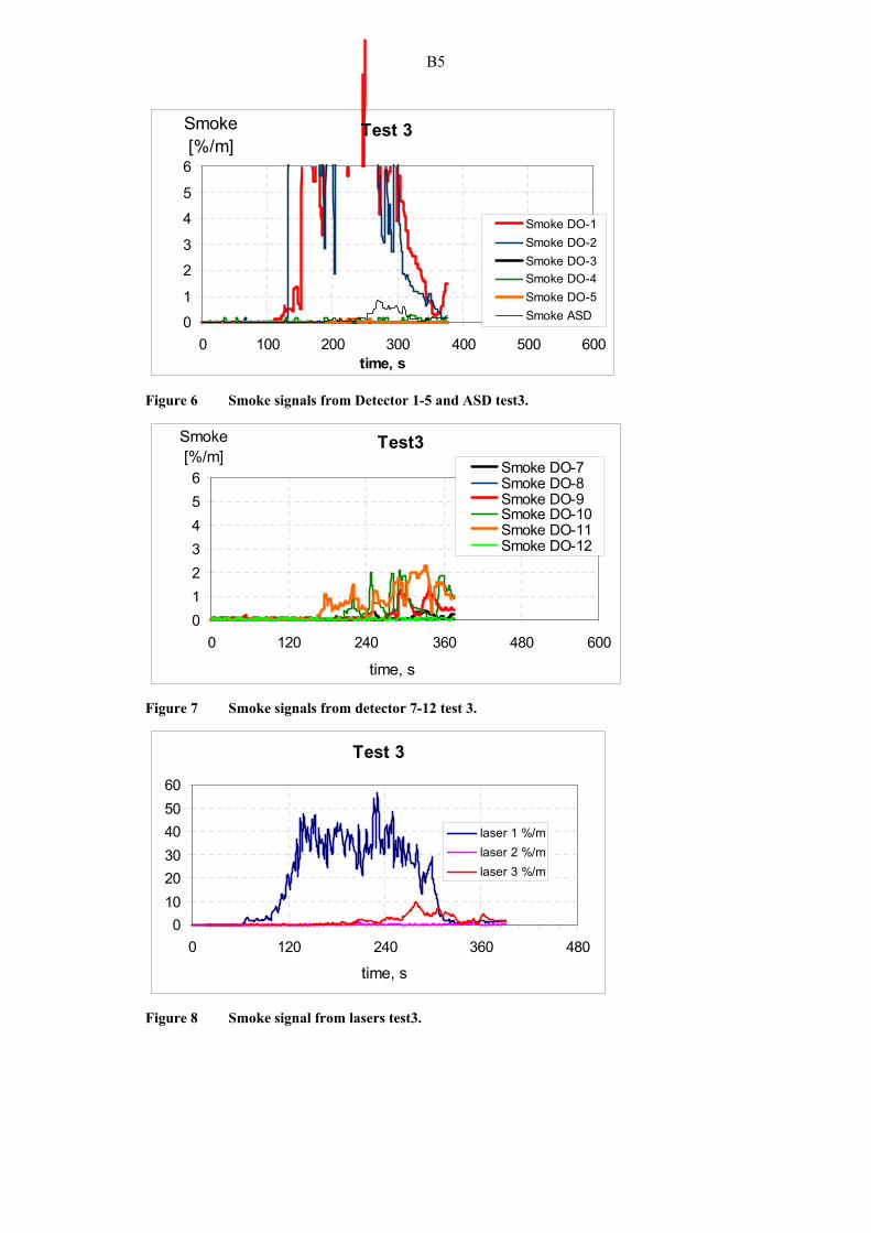
B5

Test 3

0

1

2

3

4

5

6

0 100 200 300 400 500 600time, s

Smoke [%/m]

Smoke DO-1Smoke DO-2Smoke DO-3Smoke DO-4Smoke DO-5Smoke ASD

Figure 6 Smoke signals from Detector 1-5 and ASD test3.

Test3

0123456

0 120 240 360 480 600

time, s

Smoke [%/m]


Figure 7 Smoke signals from detector 7-12 test 3.

Test 3

0102030405060

0 120 240 360 480

time, s


Figure 8 Smoke signal from lasers test3.

B6


Detector Time to warning, s Time to pre-alarm, s Time to alarm, s Detector 1 161 177 192 Detector 2 147 162 181 Detector 3 Detector 4 Detector 5 Detector 6 ASD 242 263 274 Detector 7 Detector 8 341 Detector 9 Detector 10 318 Detector 11 283 313 Detector 12

Test 4 TF2 fire with 20 wooden sticks. The heating plate was turned on at the same time as the measuring and video time started. The experiment was interrupted due to loss of power to the heating plate due to a thermo-fuse in the extension cord.

Test 4

05

1015202530

0 120 240 360 480 600time, s




Detector Time to warning, s Time to pre-alarm, s Time to alarm, s Detector 1 Detector 2 Detector 3 Detector 4 Detector 5 Detector 6 ASD 507 Detector 7 Detector 8 639 Detector 9 614

B7

Detector Time to warning, s Time to pre-alarm, s Time to alarm, s Detector 10 Detector 11 Detector 12

Test 5 TF2 fire with 20 wooden sticks. The heating plate was turned on at the same time as the measuring and video time started. The experiment was interrupted due to loss of power to the heating plate due to a thermo-fuse in the extension cord.

Test 5

0.00.51.01.52.02.53.0

0 120 240 360 480 600 720 840

time, s

Smoke [%/m]



Test5

0.0

0.5

1.0

1.5

2.0

2.5

3.0

0 120 240 360 480 600 720 840time, s

Smoke [%/m]


Figure 11 Smoke signals from detector 7-12, test5.

B8

Test5

0

10

20

30

40

0 120 240 360 480 600 720 840

time, s


Figure 12 Smoke signals from lasers, test 5.

Table 6 Time to warning, pre-alarm and alarm, test6.

Detector Time to warning, s Time to pre-alarm, s Time to alarm, s Detector 1 Detector 2 Detector 3 Detector 4 Detector 5 Detector 6 ASD 451 617 Detector 7 Detector 8 Detector 9 Detector 10 Detector 11 Detector 12

Test 6 TF2 with 24 wooden sticks. Computers, video time and heating plate started at same time. The experiment was interrupted after the wooden sticks started to flame.

B9

Test 6

0.0

0.5

1.0

1.5

2.0

2.5

3.0

0 120 240 360 480 600 720 840 960

time, s

Smoke [%/m]



Test 6

0.00.51.01.52.02.53.0

0 120 240 360 480 600 720 840 960time, s

Smoke [%/m]

Smoke DO-7Smoke DO-8Smoke DO-9Smoke DO-10Smoke DO-11Smoke DO-12Smoke DO-14

Figure 14 Smoke signals from detector 7-14, test 6.

Test 6

0

10

20

30

40

50

0 120 240 360 480 600 720 840 960

time, s



B10

Table 7 Time to warning, pre-alarm and alarm, test6.

Detector Time to warning, s Time to pre-alarm, s Time to alarm, s Detector 1 Detector 2 Detector 3 Detector 4 Detector 5 Detector 6 ASD Detector 7 Detector 8 Detector 9 Detector 10 Detector 11 Detector 12 Detector 14 604

Test 7 SG3000. 30 s pre-measuring time. Video started at same time as smoke generator.

Test 7

0.00.51.01.52.02.53.0

0 100 200 300 400 500 600 700 800 900time, s

Smoke [%/m]


Figure 16 Smoke signals from detector 1-6 and ASD, test7

Test 7

0.01.02.03.04.05.06.0

0 120 240 360 480 600 720time, s

Smoke [%/m]



B11

Test 7

01020304050607080

0 120 240 360 480 600 720time, s



Table 8 Time to warning pre-alarm and alarm, test 7.

Detector Time to warning, s Time to pre-alarm, s Time to alarm, s Detector 1 Detector 2 Detector 3 Detector 4 Detector 5 Detector 6 ASD 182 270 286 Detector 7 420 435 Detector 8 Detector 9 341 411 Detector 10 252 350 410 Detector 11 423 Detector 12 201 Detector 14 111 126 154

Test 8 AG2000 with the paraffin oil from SG3000. This did not work very well, very little smoke was produced.

Test 9 AG2000 with disco fluid. Interrupted due to ignition off leftovers from the paraffin oil.

B12

Test 10 AG2000 with 50 ml of disco fluid, about 3-4 drops per second, 4.6 kW heating power. 30 s of pre-measuring time. The liquid lasted for 6 min and 15 s.

Test 10

0

2

4

6

8

10

12

0 120 240 360 480 600 720time, s

Smoke [%/m]



Test 10

0123456

0 120 240 360 480 600 720time, s

Smoke [%/m] Smoke DO-7


Figure 20 Smoke signals detector 7-14, test 10.

Test 10

0

20

40

60

80

0 120 240 360 480 600 720

time, s



B13

Table 9 Time to warning, pre-alarm and alarm, test 10.

Detector Time to warning, s Time to pre-alarm, s Time to alarm, s Detector 1 91 152 167 Detector 2 81 203 227 Detector 3 Detector 4 Detector 5 Detector 6 ASD 119 171 183 Detector 7 356 414 Detector 8 353 Detector 9 354 393 Detector 10 249 264 391 Detector 11 374 Detector 12 367 Detector 14 351

Test 11 AG2000 with 70 g of small pieces of PE-box. Heating power 2.2 kW. Pre-measuring time 31 s, the video time started at the same time as computers. The heating power was in-creased to 4.6 at time 18 minutes.

Test 11

01

234

56

0 300 600 900 1200 1500time, s

Smoke [%/m]


Figure 22 Smoke signals from detectors 1-6 and ASD, test 11.

B14

Test 11

0

1

2

3

4

5

6

0 300 600 900 1200 1500time, s

Smoke [%/m]


Figure 23 Smoke signals from detectors 7-14, test 11.

Test 11

0102030405060

0 240 480 720 960 1200 1440

time, s




Detector Time to warning, s Time to pre-alarm, s Time to alarm, s Detector 1 734 749 768 Detector 2 736 758 773 Detector 3 Detector 4 Detector 5 Detector 6 ASD 799 811 826 Detector 7 912 Detector 8 931 Detector 9 937 Detector 10 902 917 956 Detector 11 805 887 908 Detector 12 805 820 893 Detector 14 794 821 855

B15

Test 12 AG2000 with 24 TF2 wooden sticks, heating power 2.2 kW. Pre-measuring time 31 s. The video time was started at the same time as the computers. Parts of the video are miss-ing due to change of batteries in the video.

Test 12

0

1

2

3

4

5

6

0 120 240 360 480 600 720 840 960 1080time, s

Smoke [%/m]



Test 12

0

1

2

3

4

5

6

0 120 240 360 480 600 720 840 960 1080time, s

Smoke [%/m]



Test12

05

101520253035

0 120 240 360 480 600 720 840 960 1080time, s



B16


Detector Time to warning, s Time to pre-alarm, s Time to alarm, s Detector 1 525 540 789 Detector 2 439 633 700 Detector 3 Detector 4 Detector 5 Detector 6 ASD 474 602 620 Detector 7 866 Detector 8 Detector 9 799 Detector 10 791 Detector 11 672 Detector 12 621 Detector 14 568 732

Test 13 TF2 plate with 24 wooden sticks. The fire was moved about 1 meter to the right com-pared to the other tests. Pre-measuring time 30 s, video start at same time as heat was turned on. Wooden sticks ignited at time 10.45 i.e. 10.15 after heat of plate was turned on. The smoke took another route this time, more to the left.

Test 13

0.00.51.01.52.02.53.0

0 120 240 360 480 600 720 840time, s

Smoke [%/m]



B17

Test 13

0.0

0.5

1.01.5

2.0

2.5

3.0

0 120 240 360 480 600 720 840time, s

Smoke [%/m]



Test 13

05

1015202530

0 120 240 360 480 600 720 840

time, s


Figure 30 Laser smoke signals, test 13.


Detector Time to warning, s Time to pre-alarm, s Time to alarm, s Detector 1 Detector 2 Detector 3 543 Detector 4 609 Detector 5 Detector 6 ASD 476 501 598 Detector 7 Detector 8 Detector 9 Detector 10 Detector 11 Detector 12 Detector 14 648

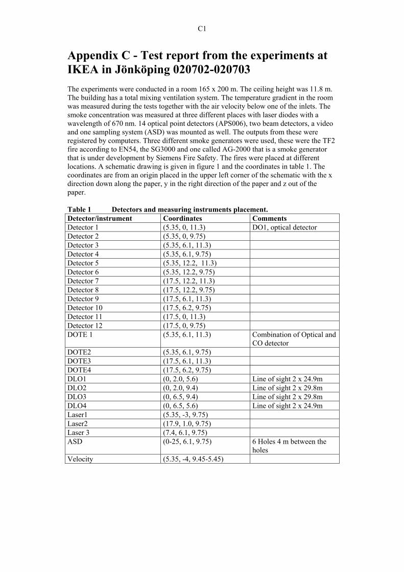
C1

Appendix C - Test report from the experiments at IKEA in Jönköping 020702-020703 The experiments were conducted in a room 165 x 200 m. The ceiling height was 11.8 m. The building has a total mixing ventilation system. The temperature gradient in the room was measured during the tests together with the air velocity below one of the inlets. The smoke concentration was measured at three different places with laser diodes with a wavelength of 670 nm. 14 optical point detectors (APS006), two beam detectors, a video and one sampling system (ASD) was mounted as well. The outputs from these were registered by computers. Three different smoke generators were used, these were the TF2 fire according to EN54, the SG3000 and one called AG-2000 that is a smoke generator that is under development by Siemens Fire Safety. The fires were placed at different locations. A schematic drawing is given in figure 1 and the coordinates in table 1. The coordinates are from an origin placed in the upper left corner of the schematic with the x direction down along the paper, y in the right direction of the paper and z out of the paper. Table 1 Detectors and measuring instruments placement. Detector/instrument Coordinates Comments Detector 1 (5.35, 0, 11.3) DO1, optical detector Detector 2 (5.35, 0, 9.75) Detector 3 (5.35, 6.1, 11.3) Detector 4 (5.35, 6.1, 9.75) Detector 5 (5.35, 12.2, 11.3) Detector 6 (5.35, 12.2, 9.75) Detector 7 (17.5, 12.2, 11.3) Detector 8 (17.5, 12.2, 9.75) Detector 9 (17.5, 6.1, 11.3) Detector 10 (17.5, 6.2, 9.75) Detector 11 (17.5, 0, 11.3) Detector 12 (17.5, 0, 9.75) DOTE 1 (5.35, 6.1, 11.3) Combination of Optical and

CO detector DOTE2 (5.35, 6.1, 9.75) DOTE3 (17.5, 6.1, 11.3) DOTE4 (17.5, 6.2, 9.75) DLO1 (0, 2.0, 5.6) Line of sight 2 x 24.9m DLO2 (0, 2.0, 9.4) Line of sight 2 x 29.8m DLO3 (0, 6.5, 9.4) Line of sight 2 x 29.8m DLO4 (0, 6.5, 5.6) Line of sight 2 x 24.9m Laser1 (5.35, -3, 9.75) Laser2 (17.9, 1.0, 9.75) Laser 3 (7.4, 6.1, 9.75) ASD (0-25, 6.1, 9.75) 6 Holes 4 m between the

holes Velocity (5.35, -4, 9.45-5.45)

C2

Figure 1 Schematic of detector and fire placement.

Smoke and CO output from detectors and lasers In all 10 experiments were conducted. Below is each experiment described and curves presented. For each experiment are the laser signals presented together with the signals from the 12 DOs and the sampling system, the smoke and CO from the DOTE and the light extinction from the beam detectors. Test1. SG3000 placed at (9.6, 5.5, 0). Pre-measuring time 30 s, measurements ended after 14 minutes.

C3

test 1

00.5

11.5

22.5

33.5

0 120 240 360 480 600 720 840 960

time, s

%/m Smoke DO-1Smoke DO-2Smoke DO-3Smoke DO-4Smoke DO-5Smoke DO-6Smoke DO-7

Figure 1 Smoke signals from detector 1-7, test 1

test 1

0

0.5

1

1.5

2

2.5

3

0 120 240 360 480 600 720 840 960

time, s

%/mSmoke DO-8Smoke DO-9Smoke DO-10Smoke DO-11Smoke DO-12Smoke ASD

Figure 2 Smoke signals from detector 8-12 and ASD, test1.

test 1

012345678

0 120 240 360 480 600 720 840 960time, s



C4

test 1

0

0.5

1

1.5

2

2.5

0 120 240 360 480 600 720 840 960

time, s

%/m

Smoke DOTE-1 Smoke DOTE-2 Smoke DOTE-3 Smoke DOTE-4

Figure 4 Smoke signals from the DOTEs, test 1.

test 1

0

0.2

0.4

0.6

0.8

1

0 120 240 360 480 600 720 840 960

time, s

ppm

CO DOTE-1 CO DOTE-2 CO DOTE-3 CO DOTE-4

Figure 5 CO signals from the DOTEs, test1.

test 1

0

20

40

60

80

100

120

0 120 240 360 480 600 720 840 960

time, s

%

Extinc. DLO-1 Extinc. DLO-2 Extinc. DLO-3 Extinc. DLO-4

Figure 6 Smoke signals from the beam detectors, test1.

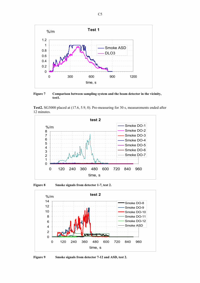
C5

Test 1

00.20.40.60.8

11.2

0 300 600 900 1200

time, s

%/m

Smoke ASDDLO3

Figure 7 Comparison between sampling system and the beam detector in the vicinity,

test1.

Test2. SG3000 placed at (17.6, 5.9, 0). Pre-measuring for 30 s, measurements ended after 12 minutes.

test 2

012345678

0 120 240 360 480 600 720 840 960time, s

%/m Smoke DO-1Smoke DO-2Smoke DO-3Smoke DO-4Smoke DO-5Smoke DO-6Smoke DO-7


test 2

02468

101214

0 120 240 360 480 600 720 840 960

time, s

%/m



C6

test 2

0246

81012

0 200 400 600 800

time, s



test 2

0123456789

0 120 240 360 480 600 720 840 960

time, s

%/m


Figure 11 Smoke signals from DOTEs, test2.

test 2

0

0.2

0.4

0.6

0.8

1

0 120 240 360 480 600 720

time, s

ppmCO DOTE-1 CO DOTE-2 CO DOTE-3 CO DOTE-4

Figure 12 CO signals from DOTEs, test2.

C7

test 2

0

20

40

60

80

100

120

0 120 240 360 480 600 720 840 960

time, s

%/m


Figure 13 Smoke signals from beam detectors, test 2.

Test 2

0

0.2

0.4

0.6

0.8

1

0 300 600 900 1200

time, s

%/m

Smoke ASDDLO3

Figure 14 Comparison between ASD and the beam detector in the vicinity, test2.

Test 3. SG3000 placed at (17.7, -2.6, 0) i.e. in the corridor with to the thermocouple tree in the vicinity of one of the air outlets. Pre-measuring time 30 s. Measurements ended after 10 and a half minutes. The smoke plume turned away from the air outlet.

test 3

0

0.05

0.1

0.15

0.2

0 120 240 360 480 600 720 840 960

time, s

%/mSmoke DO-1Smoke DO-2Smoke DO-3Smoke DO-4Smoke DO-5Smoke DO-6Smoke DO-7

Figure 15 Smoke signals from detectors 1-7, test3.

C8

test 3

0

0.5

1

1.5

2

0 120 240 360 480 600 720 840 960

time, s

%/m Smoke DO-8Smoke DO-9Smoke DO-10Smoke DO-11Smoke DO-12Smoke ASD

Figure 16 Smoke signals from detectors 8-12 ans ASD, test3.

test 3

0

2

4

6

8

0 200 400 600 800

time, s



test 3

0

0.05

0.1

0.15

0.2

0.25

0 120 240 360 480 600 720 840 960

time, s

%/m


Figure 18 Smoke signals from DOTEs test3.

C9

test 3

0

0.2

0.4

0.6

0.8

1

0 120 240 360 480 600 720

time, s

ppm


Figure 19 CO signal from DOTEs test3.

test 3

0

20

40

60

80

100

120

0 120 240 360 480 600 720

time, s

%


Figure 20 Smoke signal from beam detectors, test3.

Test 3

0

0.1

0.2

0.3

0.4

0.5

0 300 600 900 1200time, s

%/m

Smoke ASDDLO3

Figure 21 Comparison between the sampling system and the beam detector in the vicinty.

C10

Test 4. SG3000 placed at (11.0, -2.4, 0) i.e. in the corridor close to the equipment room. Pre-measuring time was about 30 s, measurement ended around 13 minutes. The plume rises straight up. Unfortunately the data-file from the laser measurements was corrupt.

test 4

00.050.1

0.150.2

0.250.3

0.35

0 120 240 360 480 600 720 840 960

time, s

%/m



test 4

01234567

0 120 240 360 480 600 720 840 960

time, s

%/m Smoke DO-8Smoke DO-9Smoke DO-10Smoke DO-11Smoke DO-12Smoke ASD

Figure 23 Smoke signals from detector 8-12 and ASD, test.

test 4

00.10.20.30.40.50.60.70.8

0 120 240 360 480 600 720 840

time, s

%/m



C11

test 4

0

0.2

0.4

0.6

0.8

1

0 120 240 360 480 600 720 840

time, s

ppm



test 4

0

20

40

60

80

100

120

0 120 240 360 480 600 720 840

time, s

%


Figure 26 Smoke signals from beam detectors, test4.

Test 4

00.10.20.30.40.50.60.7

0 300 600 900 1200

time, s

%/m

Smoke ASDDLO3

Figure 27 Comparison between sampling system and the beam detector in the vicinity.

C12

Test 5. TF2 with the new type of wooden sticks placed at (9.0, 5.5, 0). The heating plate was started after 40 s of pre-measuring time. Smoke started to emerge at 3 minutes and 40 s. A power failure to the heating plate occurred at 10 minutes and 50 s. Power came back at time 12 minutes and 20 seconds. The wooden sticks self ignited at time 16 minutes and 20 s. Measurements ended at 18 minutes and 30 s. More alarms occurred in this test than in the previous ones.

test 5

0

2

4

6

8

10

12

0 300 600 900 1200 1500

time, s


Figure 28 Smoke signals from detector 1-7 test5.

test 5

0

0.5

1

1.5

2

0 300 600 900 1200 1500

time, s

%/m


Figure 29 Smoke signals from detectors 8-12 and ASD, test 5.

test 5

0

5

10

15

20

0 120 240 360 480 600 720 840 960 1080 1200

time, s



C13

test 5

0

24

68

1012

14

0 120 240 360 480 600 720 840 960 1080 1200

time, s

%/m



test 5

0

2

4

6

8

10

0 120 240 360 480 600 720 840 960 1080 1200

time, s

ppm


Figure 32 CO signals from DOTEs test5.

test 5

0

20

40

60

80

100

120

0 120 240 360 480 600 720 840 960 1080 1200

time, s

%



C14

Test 5

00.20.40.60.8

11.21.4

0 300 600 900 1200 1500

time, s

%/m

Smoke ASDDLO3

Figure 34 Comparison between ASD and the beam detector in the vicinity.

Test 6. AG2000 with 10 wooden sticks of the new type at 2.2 kW placed at (9.0, 5.5, 0). Pre-measuring time 30 s. The power was increased to 4.6 kW at 18 minutes. Measure-ments ended at 20 minutes.

test 6

0

2

4

6

8

10

12

0 120 240 360 480 600 720 840 960 1080 1200 1320

time, s



test 6

00.10.20.30.40.50.60.7

0 300 600 900 1200 1500 1800

time, s



C15

test 6

0

5

10

15

20

25

30

0 120 240 360 480 600 720 840 960 1080 1200 1320

time, s


Figure 37 Smoke signals lasers, test6.

test 6

0

2

4

6

8

10

12

0 120 240 360 480 600 720 840 960 1080 1200

time, s

%/m


Figure 38 Smoke signals from DOTEs test6.

test 6

0

0.2

0.4

0.6

0.8

1

1.2

1.4

0 120 240 360 480 600 720 840 960 1080 1200

time, s

ppm



C16

test 6

0

20

40

60

80

100

120

0 120 240 360 480 600 720 840 960 1080 1200

time, s

%


Figure 40 Smoke signals from beam detector, test6.

Test 6

0

0.2

0.4

0.6

0.8

1

1.2

0 120 240 360 480 600 720 840 960 1080 1200

time, s

%/m

Smoke ASDDLO3

Figure 41 Comparison between sampling system and the beam detector in the vicinity.

Test 7. AG2000 with 24 small wooden sticks, 2.2 kW, at (12.6, 5.3, 0). Pre-measuring time 30 s.

test 7

0

0.05

0.1

0.15

0.2

0.25

0 120 240 360 480 600 720 840 960 1080

time, s

%/m Smoke DO-1

Smoke DO-2Smoke DO-3

Smoke DO-4

Smoke DO-5

Smoke DO-6Smoke DO-7


C17

test 7

00.10.20.30.40.50.60.70.8

0 120 240 360 480 600 720 840 960

time, s

%/m



test 7

00.050.1

0.150.2

0.250.3

0.35

0 120 240 360 480 600 720 840 960 1080 1200time, s


Figure 44 Laser smoke signals test 7.

test 7

0

0.05

0.1

0.15

0.2

0.25

0.3

0 120 240 360 480 600 720 840 960 1080 1200

time, s

%/mSmoke DOTE-1

Smoke DOTE-2

Smoke DOTE-3

Smoke DOTE-4


C18

test 7

0

1

2

3

4

5

0 120 240 360 480 600 720 840 960 1080 1200

time, s

ppm


Figure 46 CO signals test7.

test 7

0

20

40

60

80

100

120

0 120 240 360 480 600 720 840 960 1080 1200

time, s

%



Test 7

0

0.2

0.4

0.6

0.8

1

0 120 240 360 480 600 720 840 960 1080 1200time, s

%/m

Smoke ASDDLO3

Figure 48 Comparison between sampling system and the beam detector nearby.

Test 8. AG2000 with 24 small wooden sticks at 4.6 kW placed at (12.6, 5.3, 0). Pre-measuring time was 30 s. IKEAs own detectors gave alarm at 8 minutes and 40 s and at 13 minutes and 40 s. The AG2000 was turned off at 12 minutes and 30 s. The measure-ments ended at 13 minutes and 30 s.

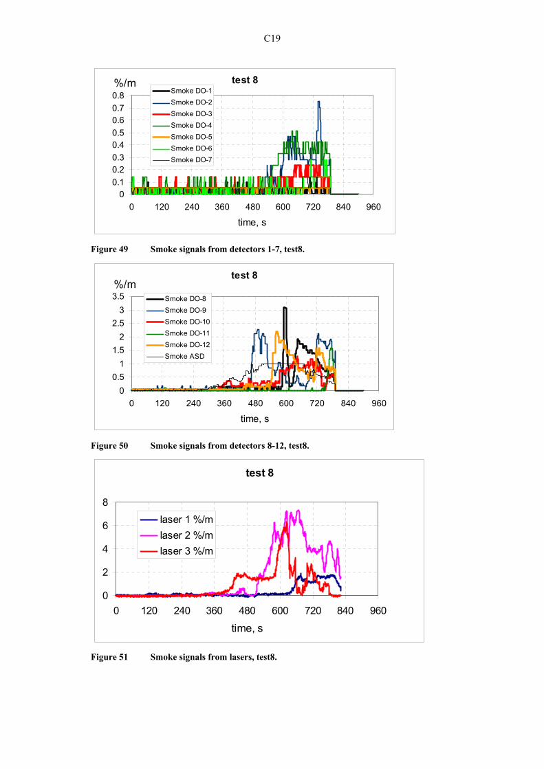
C19

test 8

00.10.20.30.40.50.60.70.8

0 120 240 360 480 600 720 840 960

time, s



test 8

00.5

11.5

22.5

33.5

0 120 240 360 480 600 720 840 960

time, s



test 8

0

2

4

6

8

0 120 240 360 480 600 720 840 960

time, s



C20

test 8

0

0.5

1

1.5

2

2.5

3

0 120 240 360 480 600 720 840 960time, s

%/m



test 8

0

0.5

1

1.5

2

2.5

3

0 120 240 360 480 600 720 840

time, s

ppm


Figure 53 CO signals, test 8.

test 8

0

20

40

60

80

100

120

0 120 240 360 480 600 720 840 960time, s

%



C21

Test 8

0

0.5

1

1.5

2

0 120 240 360 480 600 720 840 960time, s

%/m

Smoke ASDDLO3

Figure 55 Comparison between sampling system and the beam detector nearby, test8.

Test 9. AG2000 with 70 g of PE-box at 4.6 kW at (12.6, 5.3, 0). IKEAs first detector gave alarm at 8 minutes and 20 s, the second after 15 minutes.

test 9

0

0.05

0.1

0.15

0.2

0.25

0.3

0.35

0 120 240 360 480 600 720 840 960

time, s



test 9

00.5

11.5

22.5

33.5

0 120 240 360 480 600 720 840 960

time, s


Figure 57 Smoke signals from detectors 8-12 and ASD, test9.

C22

test 9

02468

101214

0 120 240 360 480 600 720 840 960

time, s



test 9

00.20.40.60.8

11.21.41.6

0 120 240 360 480 600 720 840 960

time, s

%/m



test 9

0

0.5

1

1.5

2

0 120 240 360 480 600 720 840 960

time, s

%/m


Figure 60 CO signals, test9.

C23

test 9

0

20

40

60

80

100

120

0 120 240 360 480 600 720 840 960time, s

%


Figure 61 Smoke signals from beam detector, test9.

Test 9

0

0.5

1

1.5

2

0 120 240 360 480 600 720 840 960time, s

%/m

Smoke ASDDLO3

Figure 62 Comparison between sampling system and the beam detector nearby.

Test 10. SG3000 at the roof of the equipment room below an air outlet at (5.35, -4, 4). Pre-measuring time 30 s. Measurements ended after almost 14 minutes.

test 10

0

0.2

0.4

0.6

0.8

1

1.2

0 120 240 360 480 600 720 840 960time, s



C24

test 10

00.050.1

0.150.2

0.250.3

0.350.4

0 120 240 360 480 600 720 840 960

time, s

%/m


Figure 64 Smoke signals from detector 8-12 and sampling system, test 10.

test 10

00.5

11.5

22.5

33.5

0 120 240 360 480 600 720 840 960

time, s



test 10

00.05

0.10.15

0.20.25

0.30.35

0.4

0 120 240 360 480 600 720 840 960time, s

%/m


Figure 66 Smoke signals from DOTEs, test 10.

C25

test 10

0

0.2

0.4

0.6

0.8

1

0 120 240 360 480 600 720 840 960time, s

ppm


Figure 67 CO signals test 10.

test 10

0

20

40

60

80

100

120

0 120 240 360 480 600 720 840 960

time, s

%


Figure 68 Smoke signals from the beam detectors, test 10.

Test 10

0

0.1

0.2

0.3

0.4

0.5

0 120 240 360 480 600 720 840 960time, s

%/m

Smoke ASDDLO3

Figure 69 Comparison between the sampling system and the nearby beam detector,

test 10.

C26

Time to warning, pre-alarm and alarm Time to warning (=DL1)m time to pre-alarm (=DL2) and time to alarm for each test is given in table 2. The time reported is from onset of fire. Table 2 Time to warning (DL1), time to pre-alarm (DL2) and time to alarm (DL3)

for the tests, time is from onset of fire Test 1 Test 2 Test 3 Test 4 Test 5 DO /

APS DL1 DL2 DL3 DL1 DL2 DL3 DL1 DL2 DL3 DL1 DL2 DL3 DL1 DL2 DL3 1/006 - - - - - - - - - - - - 653 668 990 2/006 402 - - - - - - - - - - - 649 664 - 3/006 - - - - - - - - - - - - 577 602 617 4/006 435 - - - - - - - - - - - 581 597 702 5/006 - - - - - - - - - - - - - - - 6/006 - - - - - - - - - - - - - - - 7/006 - - - 154 242 381 - - - - - - - - - 8/006 429 450 - 460 - - - - - - - - - - - 9/006 - - - 81 136 242 - - - - - - - - -

10/006 441 - - 148 175 242 - - - 485 533 - 948 - - 11/006 - - - 217 - - 161 - - 251 275 366 - - - 12/006 - - - - - - 64 - - 538 - - - - -

DOTE1 - - - - - - - - - - - - 610 622 - DOTE2 - - - - - - - - - - - - 599 610 696 DOTE3 - - - 116 229 238 - - - - - - - - - DOTE4 - - - 180 226 235 - - - - - - - - -

DLO1 - - - - - - - - - - - - - - - DLO2 289 301 383 225 246 298 241 374 - 182 252 319 - - - DLO3 196 205 264 237 313 - - - - 411 420 - 445 463 502 DLO4 - - - 269 325 - - - - - - - 447 447 490

ASD 43 55 67 63 90 120 206 392 422 242 318 330 406 421 448

Test 6 Test 7 Test 8 Test 9 Test 10 DO / APS DL1 DL2 DL3 DL1 DL2 DL3 DL1 DL2 DL3 DL1 DL2 DL3 DL1 DL2 DL3

1/006 633 649 667 - - - - - - - - - - - - 2/006 720 - - - - - - - - - - - - - - 3/006 597 615 633 - - - - - - - - - - - - 4/006 595 613 628 - - - - - - - - - - - - 5/006 - - - - - - - - - - - - - - - 6/006 - - - - - - - - - - - - - - - 7/006 - - - - - - - - - - - - - - - 8/006 - - - - - - 571 - - 498 - - - - - 9/006 - - - - - - 450 478 - 672 - - - - -

10/006 - - - - - - 600 - - 475 534 - - - - 11/006 - - - - - - 740 - - - - - - - - 12/006 - - - - - - 528 - - 682 - - - - -

DOTE1 607 619 631 - - - 596 641 - 685 - - - - - DOTE2 621 631 640 - - - - - - - - - - - - DOTE3 - - - - - - - - - - - - - - - DOTE4 - - - - - - - - - - - - - - -

DLO1 - - - - - - - - - - - - - - - DLO2 628 644 650 705 737 - 411 414 426 428 455 485 458 - - DLO3 592 592 626 581 611 690 348 369 393 369 374 395 541 - - DLO4 592 607 - 662 668 - - - - - - - - - -

ASD 593 611 624 498 571 647 278 305 342 343 361 373 443 525

C27

Temperature and velocity The temperature distribution and velocity below the air inlet did not vary much between tests as expected, the curves from test 1, 5 and 10 are presented in below. The straight line for velocity 1, closest to the inlet is due to that the velocity is higher then the measurement range for the meter, i.e. 2.6 m/s.

test 1

16

16.5

17

17.5

18

18.5

0 120 240 360 480 600 720 840 960

time, s

°CIMP4/Ch1 degCIMP4/Ch2 degCIMP4/Ch3 degCIMP4/Ch4 degCIMP4/Ch5 degCIMP4/Ch6 degCIMP4/Ch7 degCIMP4/Ch8 degCIMP4/Ch9 degCIMP4/Ch10 degCIMP4/Ch11 degC

Figure 70 Temperature distribution test1.

test 1

00.5

11.5

22.5

3

0 120 240 360 480 600 720 840 960

time, s

m/s

vel1 m/s

vel2 m/s

vel3 m/s

vel4 m/s

vel5 m/s

Figure 71 Velocity below an air inlet test1.

test 5

1616.216.416.616.8

1717.217.417.6

0 300 600 900 1200

time, s

°C

IMP4/Ch1 degC

IMP4/Ch2 degCIMP4/Ch3 degC

IMP4/Ch4 degC




IMP4/Ch11 degC

Figure 72 Temperature distribution test5.

C28

test 5

00.5

11.5

22.5

3

0 120 240 360 480 600 720 840 960 1080 1200

time, s

m/s

vel1 m/s

vel2 m/s

vel3 m/s

vel4 m/s

vel5 m/s

Figure 73 Velocity below an air inlet test5.

test 10

16

16.5

17

17.5

18

18.5

19

0 120 240 360 480 600 720 840 960

time, s

°C

IMP4/Ch1 degC

IMP4/Ch2 degC

IMP4/Ch3 degC

IMP4/Ch4 degC

IMP4/Ch5 degC

IMP4/Ch6 degC

IMP4/Ch7 degC

IMP4/Ch8 degC

IMP4/Ch9 degC

IMP4/Ch10 degC

IMP4/Ch11 degC

Figure 74 Temperature distribution test 10.

test 10

00.5

11.5

22.5

3

0 120 240 360 480 600 720 840 960time, s

m/s

vel1 m/s

vel2 m/s

vel3 m/s

vel4 m/s

vel5 m/s

Figure 75 Velocity below an air inlet, test10.

SP Swedish National Testing and Research InstituteBox 857SE-501 15 BORÅS, SWEDENTelephone: + 46 33 16 50 00, Telefax: +46 33 13 55 02E-mail: [email protected], Internet: www.sp.se

SP S

wed

ish

Nat

ion

al T

esti

ng

an

d R

esea

rch

Inst

itu

te



SP Fire TechnologySP REPORT 2003:33

SP Fire TechnologySP REPORT 2003:33ISBN 91-7848-971-7ISSN 0284-5172

SP Swedish National Testing and Research Institute develops and transfers

technology for improving competitiveness and quality in industry, and for safety,

conservation of resources and good environment in society as a whole. With

Swedens widest and most sophisticated range of equipment and expertise for

technical investigation, measurement, testing and certfi cation, we perform

research and development in close liaison with universities, institutes of technology

and international partners.

SP is a EU-notifi ed body and accredited test laboratory. Our headquarters are in

Borås, in the west part of Sweden.

smoke detection in buildings with high ceilings - rise · stage of the fire, i.e. when it is only...

Documents