smooth scheduling for electricity distribution in the …szm0001/papers/isj_2045.final.pdfhuanget...

966 IEEE SYSTEMS JOURNAL, VOL. 9, NO. 3, SEPTEMBER 2015

Smooth Scheduling for Electricity Distributionin the Smart Grid

Yingsong Huang, Student Member, IEEE, Shiwen Mao, Senior Member, IEEE, and R. M. Nelms, Fellow, IEEE

Abstract—The emergence of smart grid (SG) brings about manyfundamental changes in electric power systems. In this paper, westudy the problem of smooth electric power scheduling in powerdistribution networks. We introduce an electricity supply/demandmodel that takes into account the time-varying demands and theirdeadlines. We formulate a constrained nonlinear programmingproblem and incorporate the theory of majorization to developalgorithms that can compute smoothness optimal schedules for thedeferrable load dominant system. An effective heuristic algorithmis also presented by extending the majorization-based algorithmfor the general scenario with both priority loads and deferrableloads. After obtaining the smooth power schedule, a distributeduser benefit maximization load control scheme is used to allocatethe scheduled power to individual users, while maximizing theirlevels of satisfaction. The analysis and simulation results demon-strate the efficacy of the proposed algorithms on smooth electricpower scheduling, peak power minimization, and reducing powergeneration cost.

Index Terms—Convex optimization, demand response (DR),majorization, power distribution, smart grid (SG).

I. INTRODUCTION

THE emergence of smart grid (SG) brings about many fun-damental changes in electric power systems [2]. Various

new power electronics and information techniques are greatlyadvancing the control and management of energy and resourcesin the power system. For example, solid-state transformers canrespond to signals from a facility or a household to changethe voltage and other electric characteristics. On the user side,smart meters and smart facilities pervasively empower moni-toring and controlling at all levels of power usage in responseto power supply and market price fluctuations [2]. The two-way flows of electricity and information in SG are instrumentalto the control and optimization of energy and resource alloca-tion in the grid to achieve efficient, green, and robust energysystems.

Manuscript received March 30, 2013; revised March 10, 2014 and June 30,2014; accepted July 9, 2014. Date of publication August 13, 2014; date ofcurrent version June 12, 2015. This work was supported in part by the NationalScience Foundation under Grant CNS-0953513 and through the BroadbandWireless Access and Applications Center site at Auburn University. This workwas presented in part at IEEE GLOBECOM 2012—Workshop on Smart GridCommunications: Design for Performance. Part of this work was done whenY. Huang was pursuing the Ph.D. degree in electrical and computer engineeringat Auburn University.

Y. Huang is with NetApp Inc., Pittsburgh, PA 15238 USA (e-mail:[email protected]).

S. Mao and R. M. Nelms are with the Electrical and Computer EngineeringDepartment, Auburn University, Auburn, AL 36849 USA (e-mail: [email protected]; [email protected]).

Digital Object Identifier 10.1109/JSYST.2014.2340231

In the SG paradigm, the next-generation distribution net-works are capable of allowing users to control their loads inresponse to the dynamics in the grid. Demand response (DR)is an important technique to balance the power generationand demand in the grid [3]. One of the important goals ofDR is to reduce the peak demand and smooth the powerprofile by scheduling user requests [2], [4]–[6]. With the two-way information flow among provider, users, and the market,various DR schemes based on real-time pricing and day-aheadload response concepts have been recently investigated [7]–[14]. Most of the existing DR schemes aim to maximize thesocial welfare or minimize the electricity payment under givendemand requirements. Although revealing the intrinsic connec-tion between pricing policies and DR, the problem of smoothelectric power scheduling has not been explicitly addressed,which is the key issue in DR. It is shown that the simple off-peak pricing scheme may not be effective in mitigating thedemand peak problem, because simply shifting the off-peakperiod may generate a new rebound peak [15].

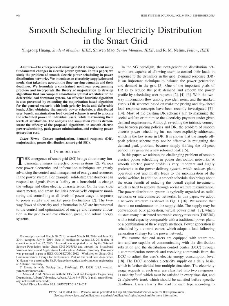
In this paper, we address the challenging problem of smoothelectric power scheduling in power distribution networks. Asmooth electric power profile is very important and highlypreferable in the power delivery system, which reduces plantoperation cost and finally leads to the maximization of thesocial welfare. In addition, a smooth schedule also brings aboutthe extra benefit of reducing the overall capital investment,which is hard to achieve through social welfare maximization.The power distribution system is typically organized as radialnetworks or interconnected networks. In this paper, we adopta network structure as shown in Fig. 1 [16]. We assume thatthere is no randomness on the supply side. The supply may beconventional bulk generation, virtual power plant [17], whichclusters many distributed renewable energy resources (DRERS)with a total capacity comparable with a traditional power plant,or a combination of these supply methods. Power generation isscheduled by a control center, which adopts a load-followinggeneration strategy for the power network.

We assume that end users are equipped with smart me-ters and are capable of communicating with the distributionsubstation and the distribution control center (DCC) througha communication network and receiving commands from theDCC to adjust the user’s electric energy consumption level[18]. The DCC schedules electricity supply on a daily basis,which is further divided into multiple time slots. The electricityusage requests at each user are classified into two categories:1) priority load, which must be satisfied in every time slot, and2) deferrable load, which should be satisfied before specificdeadlines. Users classify the load for each type according to

1932-8184 © 2014 IEEE. Personal use is permitted, but republication/redistribution requires IEEE permission.See http://www.ieee.org/publications_standards/publications/rights/index.html for more information.

HUANG et al.: SMOOTH SCHEDULING FOR ELECTRICITY DISTRIBUTION IN THE SMART GRID 967

Fig. 1. Illustration of the electricity distribution network.

their preference [e.g., lighting, entertainment, or charging aplug-in hybrid electric vehicle (PHEV)] [3]. The DCC aggre-gates the demand profiles from the users through the aggregator[19] and smooths the aggregated electric power supply underthe priority load and deferrable load deadline constraints.

The objective of the smooth electric power scheduling prob-lem is to minimize the power variation during a daily period,based on the concept of day-ahead load response. A deter-ministic electricity supply/demand model is introduced withcumulative electricity demand/supply curves, which character-ize the demand/supply relationship during the day. We findthat the formulated problem suits well with the majorizationtheory, which concerns with the comparison and ordering ofvectors with respect to the distribution of their elements [20].Majorization has been used in solving optimization problems inthe communications and networking area [21], [22]. In this pa-per, we present a majorization-based framework to develop twosmooth electric power scheduling algorithms with low com-putational complexity. Once the smooth electric power profilefor the entire network is obtained, a user benefit maximizationload control algorithm will be executed to allocate the totalamount of supply to the individual users, while maximizingtheir satisfaction of electricity usage. The proposed algorithmscan achieve the minimum peak power, thus requiring smallercapacity for the generators, transmission lines, and transformersto support the same demand. Since electrical generation andtransmission systems are generally designed to accommodatepeak electric power [2], the smooth electric power schedule alsohelps to optimize the deployment and operation cost of the grid.

This paper extends an earlier five-page conference version[1] with the following new contributions: more detailed dis-cussions, introduction of the preliminaries, an in-depth perfor-mance analysis of the proposed schemes, detailed proofs ofthe propositions and lemmas, and a comprehensive simulationevaluation of the proposed schemes. The remainder of thispaper is organized as follows. We first present the system modeland problem statement in Section II. We next provide a brief

TABLE INOTATION

introduction of majorization in Section III. The smooth electricpower scheduling algorithms are described in Section IV, andtheir performance is evaluated in Section V. Related work isdiscussed in Section VI, and Section VII concludes this paper.The notation is summarized in Table I.

II. PROBLEM STATEMENT

A. Load Demand Profile

We consider a power distribution network with two-wayflows of electricity and information. We assume N users inthe power distribution network, which may generate residential,commercial, and industrial load. Let U = {1, 2, . . . , N} be theset of users. The electric demand of a user is daily based.Without loss of generality, we assume that the one-day periodis divided into L time slots, each with length τ . Let pn(t) bethe power consumption of user n in time slot t, which is timevarying but remains constant within the time slot. Each user nknows its own total daily demand, i.e., En =

∑Lt=1 pn(t)τ , and

wishes to schedule the demand over the one-day period [12].We assume that the total demand En consists of two parts:

the priority load and the deferrable load. The priority loadshould be strictly guaranteed in a time slot (e.g., for light-ing), whereas the deferrable load can be flexibly served butwith a specific deadline (e.g., charging a household battery orPHEVs). We define en,p(t) and en,d(t) as the electric energyfor priority load in time slot t and the deferrable load that mustbe satisfied by time slot t, respectively. The minimum demand


Fig. 2. Cumulative demand and supply curves.

of user n in time slot t, which is denoted by eminn (t), is the

sum of en,p(t) and en,d(t). Finally, let emaxn (t) be the maximum

possible demand for user n, which is limited by the amount ofdeferrable loads that have not been satisfied yet and the capacityof protective relays and switches of the users.

B. Cumulative Demand and Supply Curves

At the beginning of a day, the DCC will aggregate theindividual demand profiles received by communicating withthe smart meters and smart facilities via the communicationsnetwork [18]. Let the total minimum electricity demand intime slot t be Emin(t) =

∑n∈U emin

n (t). We have Emin(L) =∑n∈U En = Φ, since the daily aggregated demand of all users,

which is denoted by Φ, should finally be satisfied by the endof the day. We define the cumulative minimum demand curve�Wmin as

Wmin(t) =

t∑l=1

Emin(l), 1 ≤ t ≤ L. (1)

We define the cumulative maximum demand curve �Wmax

to represent the maximum amount of electricity demandthat can be consumed up to t as Wmax(t) = min{Wmin(t−1) +

∑n∈U[e

maxn (t) + Δen(t− 1)],Φ}, 1 ≤ t ≤ L, where

Δen(t) = emaxn (t)− emin

n (t) is the deferrable load thatcan be served in slot t but with deadlines later than t. Toincorporate the priority load in the model, Wmax(t) alsosatisfies Wmax(t) ≥ Wmax(t− 1) +

∑n∈U en,p(t).

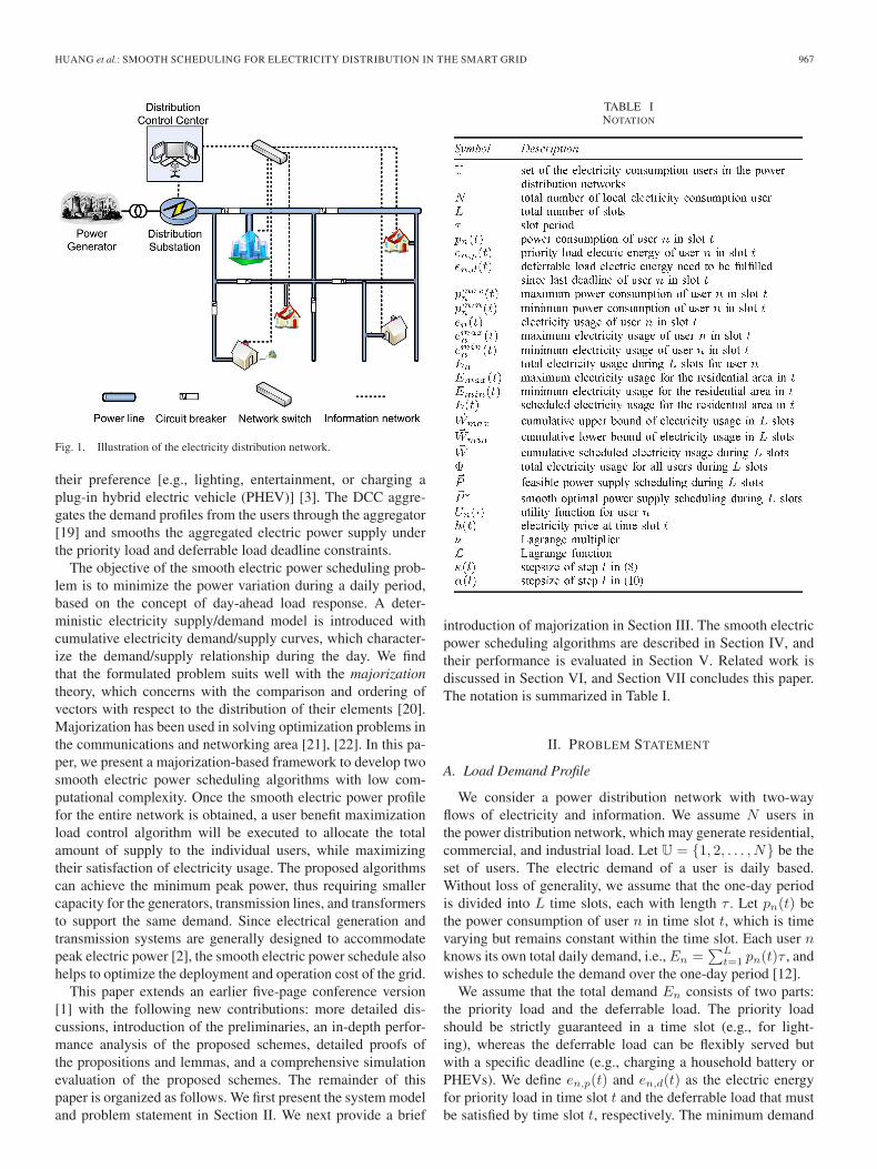
For given demand curves �Wmin and �Wmax, we aim to find afeasible electricity schedule �W , which is the cumulative supplyof electricity to the users that satisfies constraints Wmin(t) ≤W (t) ≤ Wmax(t), for all 1 ≤ t ≤ L, and W (L) = Φ (i.e., thetotal demand should be satisfied by the end of the day). Thethree cumulative curves are illustrated in Fig. 2, which are allnondecreasing over time.

The proposed demand and supply model is quite general.It does not assume any mathematical model for either thesupply or the demand. It is more practical than the complexstatistical models for supply and demand used in the literature

[2]. The cumulative curves represent the demand/supply statusin the power distribution network. In each time slot t, Wmin(t)tracks the priority load and the deferrable load with deadlinet, whereas Wmax(t) represents an upper bound of the possibleconsumption by time t. The gap between Wmax(t) and Wmin(t)may accommodate the future uncertainty of the electric powerusage. The slope of W (t), which is denoted by P (t), corre-sponds to the scheduled electric power. The DCC aims to findan optimal schedule W (t) for every time slot t to achieve aspecific control target. A feasible power supply schedule �P =[P (1), P (2), . . . , P (L)] ensures that �W lies between �Wmin and�Wmax for all the L time slots, thus preventing both outageevents and energy waste.

It is shown in Fig. 2 that the feasible electric power schedulemay not be unique. Among various feasible schedules, we areinterested in the one that distributes electricity most smoothlyamong the L time slots, i.e., the smoothness optimal schedule.Once the DCC obtains the smoothness optimal schedule, it canannounce the schedule to the smart meters and smart utilitiesat the users’ premises via the communication network, and theusers can shape their demand to match the schedule (assumingcooperative users). Therefore, we can achieve smooth electric-ity generation, transmission, and consumption, which is highlypreferable for the grid design and operation [2].

C. Smooth Power Scheduling Problem

Based on the demand and supply model, we formulatethe smooth power scheduling problem here. Let P̄ = Φ/(Lτ)be the average power consumption in the power distribu-tion network through the daily period. The scheduled powerfor each time slot is P (t) = (W (t)−W (t− 1))/τ = E(t)/τ .The smoothness optimal schedule minimizes the variations ofthe supplied power over the entire period, i.e.,

maximize : S(�P )

subject to : Wmin(t) ≤ W (t) ≤ Wmax(t), for all t

W (L) = Wmin(L) = Wmax(L) = Φ

P (t) = [W (t)−W (t− 1)] τ

≥ Ep(t)

τ, for all t (2)

where S(�P ) is the smoothness of a schedule �P , and Ep(t) =∑n∈U en,p(t) is the total priority load in time slot t.Generally, smoothness can be measured by different metrics,

such as variance and cumulative absolute difference. Eachsmoothness measure leads to a different objective function inproblem (2), whereas the solution to the problem will thendepend on the specific form of the objective function. In addi-tion, the smoothness measures are generally nonlinear, makingthe problem nontrivial to solve. In this paper, we resort tothe mathematical theory of majorization [20], which explicitlyaddresses the unique mathematical notion for smoothness. Ap-plying majorization theory, we will see that, for an arbitrarysmoothness objective function in problem (2) that satisfies theSchur-convex properties [20], the problem can be solved by


a universal algorithm in polynomial time. For brevity in thededuction, we minimize the load variance in the rest of thispaper, whereas the solution algorithms developed in Section IVapply to any objective function that is Schur-convex.

We first consider the case where the deferrable load is thedominant component [23], i.e., Ep(t) ≈ 0. Problem (2) is thenreduced to problem (3), i.e.,

minimize :L∑

t=1

[P (t)− P̄

]2/L

subject to : Wmin(t) ≤ W (t) ≤ Wmax(t), for all t

W (L) = Φ

P (t)=[W (t)−W (t− 1)]

τ, for all t. (3)

This problem fits well with the majorization theory, since theobjective function is Schur-convex [20]. We briefly review ma-jorization preliminaries in Section III. Applying majorization,we will design a smooth electric power scheduling algorithmfor solving problem (3) in Section IV-A. We will then extendthe algorithm for solving problem (2) in Section IV-C.

III. MAJORIZATION PRELIMINARIES

The majorization theory [20] describes the “less spreadingout” or the “more nearly equal” properties of the elementsof a vector comparing with the elements of another vector. Itconcerns with the problem of ordering vectors with nonnega-tive real elements, as well as order-preserving functions. Forsimplicity, all the vectors here are row vectors.

Definition 1: For two n-element vectors �X =(x1, x2, . . . , xn) and �Y = (y1, y2, . . . , yn), with elementssorted in the nonincreasing order as x1 ≥ x2 ≥ · · · ≥ xn ≥ 0and y1 ≥ y2 ≥ · · · ≥ yn ≥ 0. �X is said to be majorized by�Y , which is denoted by �X ≺ �Y , if 1)

∑ti=1 xi ≤

∑ti=1 yi,

t = 1, 2, . . . , n− 1, and 2)∑n

i=1 xi =∑n

i=1 yi [20].Definition 2: A real-valued function φ defined on a set A ⊂

Rn is said to be Schur-convex on A if �X ≺ �Y on A ⇒ φ( �X) ≤φ(�Y ) [20].

Schur-convex functions have the “order-preserving” prop-erty, which bridges majorization and optimization. Schur-convex functions can be validated with the following fact.

Fact 1: If φ is symmetric and convex, then φ is Schur-convex. Consequently, �X ≺ �Y implies φ( �X) ≤ φ(�Y ) [20].

This fact provides connection between ordering and its order-preserving functions. By this fact, we may solve the minimiza-tion problem by generating the most spreading out vector as thesolution. If φ =

∑g and g is continuous convex, then we have

the following fact.Fact 2:

∑i g(xi) ≤

∑i g(yi) ⇔ �X ≺ �Y holds for all con-

tinuous convex functions g : R → R [20].Lemma 1: Let �X = ( �X1, . . . , �XK) and �Y = (�Y1, . . . , �YK),

where each element has dimension Ji and satisfying �Xi ≺ �Yi

for all i. Then, �X ≺ �Y .Proof: Let g be the continuous convex function

R→R. By Fact 2, �Xi≺ �Yi⇔∑Ji

j=1 g(xji )≤

∑Ji

j=1 g(yji )⇒∑K

i=1

∑Ji

j=1 g(xji )≤

∑Ki=1

∑Ji

j=1 g(yji )⇔ �X ≺ �Y . �

Fig. 3. Illustration of different Lorenz curves.

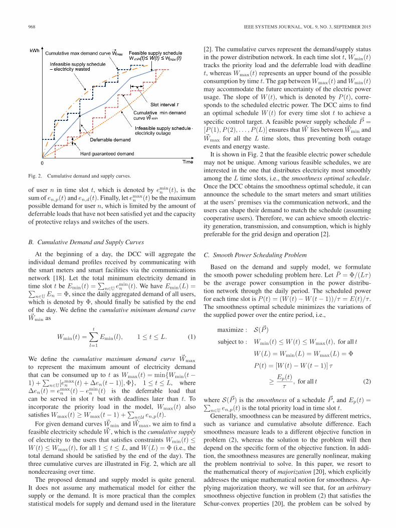
Let �X = (x̄, . . . , x̄), �Y = (y1, . . . , yn), and �Z =(z1, . . . , zn), where

∑ni=1 yi =

∑ni=1 zi = nx̄. If the elements

in each vector are nondecreasing, we can plot the normalizedpoints of �X/(nx̄), �Y /(nx̄), and �Z/(nx̄) as in Fig. 3. Theelements of vectors can be interpreted as the incomes ofindividuals, as in a Lorenz curve, which evaluates the socialincome inequality [24]. The curves show the normalizedcumulative proportion of the income versus the cumulativepercentage of population. The normalized vector �X forms astraight curve A, which corresponds to the equal distribution.Normalized vectors �Y and �Z represent unequal distributionsand bent in the middle, which is denoted by curves B and Cin the figure, respectively. We call them bow curves in theconvex shape. The more the Lorenz curve bents, the higherthe concentration of the elements; the bow curve closer to Arepresents a more even distribution [20]. From the perspectiveof majorization, we have �X ≺ �Y ≺ �Z. Similarly, we canshuffle the elements in �X/(nx̄) and �Y /(nx̄) to get two newLorenz curves B′ and C ′. We call these bow curves in theconcave shape. Since the order of the vectors plays no role inmajorization, �X ≺ �Y ≺ �Z still holds for concave curves.

Proposition 1: The objective function of problems (2) and(3) is Schur-convex. �

Proof: The proof directly follows Fact 1, due to the sym-metric and convex of the objective function in problems (2)and (3). �

IV. SMOOTH ELECTRIC POWER SCHEDULING

A. SEPS-DL Algorithm

We first develop a smooth electric power scheduling fordeferrable load (SEPS-DL) algorithm based on majorization.With Proposition 1, we convert the optimization problem (3)into an ordering problem of vectors, each representing a fea-sible schedule. Thus, we solve problem (3) by computing themost evenly distributed electric power schedule that is feasiblefor the entire period. Obviously, the most evenly distributedschedule is �P opt = [Φ/(Lτ), . . . ,Φ/(Lτ)], corresponding tohaving the average power consumption P̄ in each time slot.However, due to time-varying user demands, �P opt may not befeasible. In general, each feasible schedule is piecewise linearwith a set of power changing points, where the scheduled powerincreases or decreases to prevent outage events or electricenergy waste.


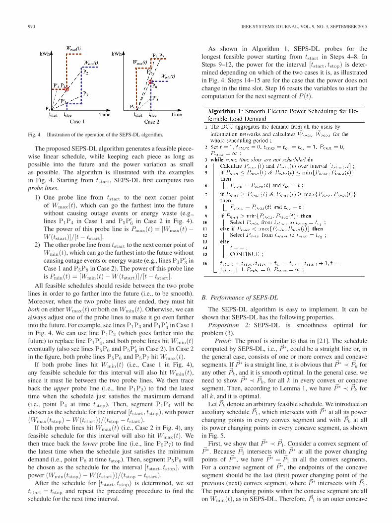
Fig. 4. Illustration of the operation of the SEPS-DL algorithm.

The proposed SEPS-DL algorithm generates a feasible piece-wise linear schedule, while keeping each piece as long aspossible into the future and the power variation as smallas possible. The algorithm is illustrated with the examplesin Fig. 4. Starting from tstart, SEPS-DL first computes twoprobe lines.

1) One probe line from tstart to the next corner pointof Wmax(t), which can go the farthest into the futurewithout causing outage events or energy waste (e.g.,lines P1P4 in Case 1 and P5P

′6 in Case 2 in Fig. 4).

The power of this probe line is Pmax(t) = [Wmax(t)−W (tstart)]/[t− tstart].

2) The other probe line from tstart to the next corner point ofWmin(t), which can go the farthest into the future withoutcausing outage events or energy waste (e.g., lines P1P

′3 in

Case 1 and P5P8 in Case 2). The power of this probe lineis Pmin(t) = [Wmin(t)−W (tstart)]/[t− tstart].

All feasible schedules should reside between the two probelines in order to go farther into the future (i.e., to be smooth).Moreover, when the two probe lines are ended, they must hitboth on either Wmax(t) or both on Wmin(t). Otherwise, we canalways adjust one of the probe lines to make it go even fartherinto the future. For example, see lines P1P3 and P1P

′4 in Case 1

in Fig. 4. We can use line P1P2 (which goes farther into thefuture) to replace line P1P

′4, and both probe lines hit Wmin(t)

eventually (also see lines P5P6 and P5P′8 in Case 2). In Case 2

in the figure, both probe lines P5P6 and P5P7 hit Wmax(t).If both probe lines hit Wmin(t) (i.e., Case 1 in Fig. 4),

any feasible schedule for this interval will also hit Wmin(t),since it must lie between the two probe lines. We then traceback the upper probe line (i.e., line P1P2) to find the latesttime when the schedule just satisfies the maximum demand(i.e., point P4 at time tstop). Then, segment P1P4 will bechosen as the schedule for the interval [tstart, tstop), with power(Wmax(tstop)−W (tstart))/(tstop − tstart).

If both probe lines hit Wmax(t) (i.e., Case 2 in Fig. 4), anyfeasible schedule for this interval will also hit Wmax(t). Wethen trace back the lower probe line (i.e., line P5P7) to findthe latest time when the schedule just satisfies the minimumdemand (i.e., point P8 at time tstop). Then, segment P5P8 willbe chosen as the schedule for the interval [tstart, tstop), withpower (Wmin(tstop)−W (tstart))/(tstop − tstart).

After the schedule for [tstart, tstop) is determined, we settstart = tstop and repeat the preceding procedure to find theschedule for the next time interval.

As shown in Algorithm 1, SEPS-DL probes for thelongest feasible power starting from tstart in Steps 4–8. InSteps 9–12, the power for the interval [tstart, tstop) is deter-mined depending on which of the two cases it is, as illustratedin Fig. 4. Steps 14–15 are for the case that the power does notchange in the time slot. Step 16 resets the variables to start thecomputation for the next segment of P (t).

B. Performance of SEPS-DL

The SEPS-DL algorithm is easy to implement. It can beshown that SEPS-DL has the following properties.

Proposition 2: SEPS-DL is smoothness optimal forproblem (3).

Proof: The proof is similar to that in [21]. The schedulecomputed by SEPS-DL, i.e., �P ∗, could be a straight line or, inthe general case, consists of one or more convex and concavesegments. If �P ∗ is a straight line, it is obvious that �P ∗ ≺ �Pk forany other �Pk, and it is smooth optimal. In the general case, weneed to show �P ∗ ≺ �Pk, for all k in every convex or concavesegment. Then, according to Lemma 1, we have �P ∗ ≺ �Pk forall k, and it is optimal.

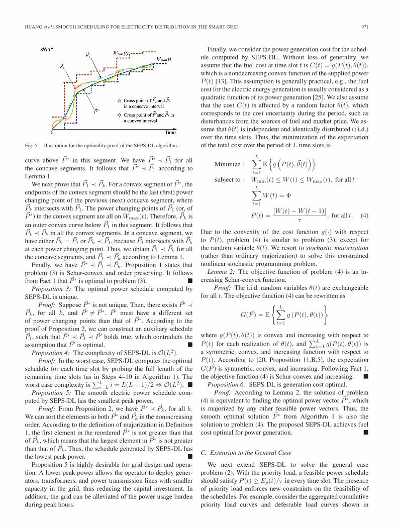
Let �Pk denote an arbitrary feasible schedule. We introduce anauxiliary schedule �P1, which intersects with �P ∗ at all its powerchanging points in every convex segment and with �Pk at allits power changing points in every concave segment, as shownin Fig. 5.

First, we show that �P ∗ ≺ �P1. Consider a convex segment of�P ∗. Because �P1 intersects with �P ∗ at all the power changingpoints of �P ∗, we have �P ∗ = �P1 in all the convex segments.For a concave segment of �P ∗, the endpoints of the concavesegment should be the last (first) power changing point of theprevious (next) convex segment, where �P ∗ intersects with �P1.The power changing points within the concave segment are allon Wmin(t), as in SEPS-DL. Therefore, �P1 is an outer concave


Fig. 5. Illustration for the optimality proof of the SEPS-DL algorithm.

curve above �P ∗ in this segment. We have �P ∗ ≺ �P1 for allthe concave segments. It follows that �P ∗ ≺ �P1 according toLemma 1.

We next prove that �P1 ≺ �Pk. For a convex segment of �P ∗, theendpoints of the convex segment should be the last (first) powerchanging point of the previous (next) concave segment, where�Pk intersects with �P1. The power changing points of �P1 (or, of�P ∗) in the convex segment are all on Wmax(t). Therefore, �Pk isan outer convex curve below �P1 in this segment. It follows that�P1 ≺ �Pk in all the convex segments. In a concave segment, wehave either �Pk = �P1 or �Pk ≺ �P1, because �P1 intersects with �Pk

at each power changing point. Thus, we obtain �P1 ≺ �Pk for allthe concave segments, and �P1 ≺ �Pk according to Lemma 1.

Finally, we have �P ∗ ≺ �P1 ≺ �Pk. Proposition 1 states thatproblem (3) is Schur-convex and order preserving. It followsfrom Fact 1 that �P ∗ is optimal to problem (3). �

Proposition 3: The optimal power schedule computed bySEPS-DL is unique.

Proof: Suppose �P ∗ is not unique. Then, there exists �P ′ ≺�Pk, for all k, and �P ′ = �P ∗. �P ′ must have a different setof power changing points than that of �P ∗. According to theproof of Proposition 2, we can construct an auxiliary schedule�P1, such that �P ∗ ≺ �P1 ≺ �P ′ holds true, which contradicts theassumption that �P ′ is optimal. �

Proposition 4: The complexity of SEPS-DL is O(L2).Proof: In the worst case, SEPS-DL computes the optimal

schedule for each time slot by probing the full length of theremaining time slots (as in Steps 4–10 in Algorithm 1). Theworst case complexity is

∑1i=L i = L(L+ 1)/2 ⇒ O(L2). �

Proposition 5: The smooth electric power schedule com-puted by SEPS-DL has the smallest peak power.

Proof: From Proposition 2, we have �P ∗ ≺ �Pk, for all k.We can sort the elements in both �P ∗ and �Pk in the nonincreasingorder. According to the definition of majorization in Definition1, the first element in the reordered �P ∗ is not greater than thatof �Pk, which means that the largest element in �P ∗ is not greaterthan that of �Pk. Thus, the schedule generated by SEPS-DL hasthe lowest peak power. �

Proposition 5 is highly desirable for grid design and opera-tion. A lower peak power allows the operator to deploy gener-ators, transformers, and power transmission lines with smallercapacity in the grid, thus reducing the capital investment. Inaddition, the grid can be alleviated of the power usage burdenduring peak hours.

Finally, we consider the power generation cost for the sched-ule computed by SEPS-DL. Without loss of generality, weassume that the fuel cost at time slot t is C(t) = g(P (t), θ(t)),which is a nondecreasing convex function of the supplied powerP (t) [13]. This assumption is generally practical, e.g., the fuelcost for the electric energy generation is usually considered as aquadratic function of its power generation [25]. We also assumethat the cost C(t) is affected by a random factor θ(t), whichcorresponds to the cost uncertainty during the period, such asdisturbances from the sources of fuel and market price. We as-sume that θ(t) is independent and identically distributed (i.i.d.)over the time slots. Thus, the minimization of the expectationof the total cost over the period of L time slots is

Minimize :

L∑t=1

E

{g(P (t), �θ(t)

)}subject to : Wmin(t) ≤ W (t) ≤ Wmax(t), for all t

L∑t=1

W (t) = Φ

P (t) =[W (t)−W (t− 1)]

τ, for all t. (4)

Due to the convexity of the cost function g(·) with respectto P (t), problem (4) is similar to problem (3), except forthe random variable θ(t). We resort to stochastic majorization(rather than ordinary majorization) to solve this constrainednonlinear stochastic programming problem.

Lemma 2: The objective function of problem (4) is an in-creasing Schur-convex function.

Proof: The i.i.d. random variables θ(t) are exchangeablefor all t. The objective function (4) can be rewritten as

G(�P ) = E

{L∑

t=1

g (P (t), θ(t))

}

where g(P (t), θ(t)) is convex and increasing with respect toP (t) for each realization of θ(t), and

∑Lt=1 g(P (t), θ(t)) is

a symmetric, convex, and increasing function with respect toP (t). According to [20, Proposition 11.B.5], the expectationG(�P ) is symmetric, convex, and increasing. Following Fact 1,the objective function (4) is Schur-convex and increasing. �

Proposition 6: SEPS-DL is generation cost optimal.Proof: According to Lemma 2, the solution of problem

(4) is equivalent to finding the optimal power vector �P ∗, whichis majorized by any other feasible power vectors. Thus, thesmooth optimal solution �P ∗ from Algorithm 1 is also thesolution to problem (4). The proposed SEPS-DL achieves fuelcost optimal for power generation. �

C. Extension to the General Case

We next extend SEPS-DL to solve the general caseproblem (2). With the priority load, a feasible power scheduleshould satisfy P (t) ≥ Ep(t)/τ in every time slot. The presenceof priority load enforces new constraints on the feasibility ofthe schedules. For example, consider the aggregated cumulativepriority load curves and deferrable load curves shown in


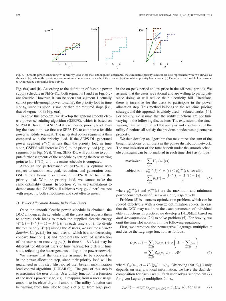
Fig. 6. Smooth power scheduling with priority load. Note that, although not deferrable, the cumulative priority load can be also represented with two curves, asshown in (a), where the maximum and minimum curves meet at each of the corners. (a) Cumulative priority load curves. (b) Cumulative deferrable load curves.(c) Aggregated cumulative load curves.

Fig. 6(a) and (b). According to the definition of feasible powersupply schedule in SEPS-DL, both segments 1 and 2 in Fig. 6(c)are feasible. However, it can be seen that segment 1 actuallycannot provide enough power to satisfy the priority load in timeslot t2, since its slope is smaller than the required slope [i.e.,that of segment 0 in Fig. 6(a)].

To solve this problem, we develop the general smooth elec-tric power scheduling algorithm (GSEPS), which is based onSEPS-DL. Recall that SEPS-DL assumes no priority load. Dur-ing the execution, we first use SEPS-DL to compute a feasiblepower schedule segment. The generated power segment is thencompared with the priority load. If the SEPS-DL generatedpower segment P ∗(t) is less than the priority load in timeslot t, GSEPS will increase P ∗(t) to the priority load [e.g., seesegment 3 in Fig. 6(c)]. Then, SEPS-DL will continue to com-pute further segments of the schedule by setting the new startingpoint to (t,W ∗(t)) until the entire schedule is computed.

Although the performance of SEPS-DL is optimal withrespect to smoothness, peak reduction, and generation cost,GSEPS is a heuristic extension of SEPS-DL to handle thepriority load. With the priority load, we cannot make thesame optimality claims. In Section V, we use simulations todemonstrate that GSEPS still achieves very good performancewith respect to both smoothness and cost effectiveness.

D. Power Allocation Among Individual Users

Once the smooth electric power schedule is obtained, theDCC announces the schedule to all the users and requests themto control their loads to match the supplied electric energyW ∗(t)−W ∗(t− 1) = P ∗(t)τ in each time slot t. To dividethe total supply W ∗(t) among the N users, we assume a benefitfunction Un(pn(t)) for each user n, which is a nondecreasingconcave function [13] and represents the level of satisfactionof the user when receiving pn(t) in time slot t. Un(t) may bedifferent for different users or time varying for different timeslots, reflecting the heterogeneous utility in the power network.

We assume that the users are assumed to be cooperativein the power allocation step, since their priority load will beguaranteed in this step [distributed user benefit maximizationload control algorithm (DUBMLC)]. The goal of this step isto maximize the user utility. User utility function is a functionof the user’s power usage, e.g., a mapping from a users’ usageamount to its electricity bill amount. The utility function canbe varying from time slot to time slot (e.g., from high price

in the on-peak period to low price in the off-peak period). Weassume that the users are rational and are willing to participatesince doing so will reduce their electricity bill. Therefore,there is incentive for the users to participate in the powerallocation step. This method belongs to the real-time pricingstrategy, and this approach is widely used in related works [14].For brevity, we assume that the utility functions are not timevarying in the following discussions. The extension to the time-varying case will not affect the analysis and conclusion, if theutility functions all satisfy the previous nondecreasing concaveproperty.

We then develop an algorithm that maximizes the sum of thebenefit functions of all users in the power distribution network.The maximization of the total benefit under the smooth sched-ule constraint can be formulated in each time slot t as follows:

maximize :∑n∈U

Un (pn(t))

subject to : pminn (t) ≤ pn(t) ≤ pmax

n (t), for alln∑n∈U

pn(t) =[W ∗(t)−W ∗(t− 1)]

τ(5)

where pmaxn (t) and pmin

n (t) are the maximum and minimumpower consumptions of user n in slot t, respectively.

Problem (5) is a convex optimization problem, which can besolved effectively with a convex optimization solver. In casethat the DCC may not know the exact parameters of individualutility functions in practice, we develop a DUBMLC based ondual decomposition [26] to solve problem (5). For brevity, weomit the time slot notation t in the following equations.

First, we introduce the nonnegative Lagrange multiplier νand derive the Lagrange function, as follows:

L(pn, ν) =∑n∈U

Un(pn) + ν

(W −

∑n∈U

pn

)

=∑n∈U

Ln(pn, ν) + νW (6)

where Ln(pn, ν) = Un(pn)− νpn. Observing that Ln(·) onlydepends on user n’s local information, we have the dual de-composition for each user n. Each user solves subproblem (7)for given Lagrange multipliers ν̃, i.e.,

pn(ν̃) = argmaxpminn ≤pn≤pmax

nLn(pn, ν̃), for alln. (7)


Subproblem (7) can be solved with the subgradient method,since Ln is strictly concave [27]. User n iteratively updates itspower pn until pn converges, as

pn(l + 1) = [pn(l) + κ(l) · ∂Ln(pn)/∂pn]+ (8)

where [·]+ denotes the projection of pn onto the range[pmin

n , pmaxn ], and κ(l) is the step size that varies in each step l

according to the Armijo rule [27]. The solution pn can be solvedlocally by the users and converges to the optimal solution of p̃nfor all n as l → ∞.

For a given optimal solution p̃n, the master dual problem isto be solved by the DCC, i.e.,

minimize : L(p̃n, ν)subject to : ν ≥ 0, for alln. (9)

We can also apply the subgradient method to iteratively updatethe multipliers as

ν(l + 1) = max {ν(l)− α(l) · ∂L(ν)/∂ν, 0} (10)

where α(l) is the step size. The Lagrange multipliers convergesto the optimal as l → ∞. Since problem (5) is a convexproblem, the duality gap is zero, and the solution of (7) isunique. The primal variable pn will also converge to the optimalsolutions [26].

The DUBMLC algorithm is presented in Algorithm 2. WithDUBMLC, each user greedily maximizes its own benefit bysolving (7) with current “price” ν, which is controlled bythe DCC through the master dual problem (9). Due to theconvexity of the problem, the optimization gap is zero, and theoptimal total maximum benefit is reached when the algorithmconverges.

Algorithm 2: Distributed User Benefit Maximization LoadControl Algorithm

1) SetAlgoLined l = 0 and the DCC initializes nonnegativeparameter ν(l);

2) The DCC announces the parameters to the users via thecommunications network;

3) Each user locally solves problem (7) as in (8) to obtain itsrequested power;

4) Each user sends its requested power to the DCC viainformation networks;

5) The DCC updates the parameters ν(l) as in (10) andannounces the new value ν(l + 1) to all users;

6) l = l + 1 and go to Step 3, until the solution converges;

Combining GSEPS and DUBMLC, we now present theGeneral Smooth Electric Power Scheduling Policy. Specifically,at the beginning of each period, which can be daily based or bean arbitrary period of time, the users send their slotted demandprofiles to the DCC through the communications network. Theusers do not need to be cooperative at this step. If a user doesnot want to shift its load, it can set all its load as priority load.

The utility company may also set an incentive to encourageusers to put more load deferrable, such as by dynamic pricing.After aggregating all the demand profiles, the DCC calculatesthe deterministic cumulative supply/demand curves for thepower distribution networks and executes GSEPS to computethe smooth power profile. After that, the DCC let the userscontrol their electricity usage to match the smooth schedulewith DUBMLC. The load control does not necessarily needto be fully executed at the exact beginning of the period. Inthe second stage, the users are assumed to be cooperative sincethey have already selected their preference at the first stage andat least all the priority load will be granted in this step. If auser requests a usage exceeding the planned service level, theDCC may allow the distribution substation to temporally fulfillthe excess demand but charging a penalty price based on theelectric energy availability of the power distribution network. Itmay operate at some time ahead of the scheduled time slot.

E. Remarks

The proposed scheme is based on two basic assumptions:1) prediction of the (near) future loads and 2) classification ofcustomer loads. It is worth noting that these are the generalassumptions made in many DR papers, where DR algorithmsare designed to intentionally modify the consumption patternsof customers’ electricity usages, such as altering the timing,the level of instantaneous demand, or the total electricityconsumption. An effective DR algorithm will shift user loadsfrom on-peak to off-peak periods depending on the consumers’preferences and lifestyles. Therefore, for DR to work, thereis a need for knowing the loads and which of the loads aredeferrable [6].

It is a challenging problem for users to perfectly predict theirfuture demand in traditional power systems. However, there arealso some facts that can be exploited for such prediction. Forexample, the electricity usage in a household usually has a dailypattern. Although there is long-term variations, the day-aheadusage is usually similar to the past-day usage. In addition, manyusages are deferrable. For example, heating may be turneddown, air conditioning or refrigeration may be turned up, andwasher and dryer/dishwasher can work in midnight, slightlydelaying the draw until a peak in usage has passed.

In the SG paradigm, with the wide deployment of smartmeters and smart appliance, it is expected that load forecastingcould be more accurate, particularly for short-term predictions(from 1 h to 1 week) [28]–[30]. The intelligent core in smartmeters can track the usage history of the users and assist users toplan the service level of each smart load/appliance and send outthe control commands with the service level of individual loadthrough networks [31]. Several energy-management start-upcompanies, such as Retroficiency, EcoFactor, and AutoGrid, areoffering effective algorithms to crunch the energy usage data sousers ranging from huge factories to individual households cantrack and reduce waste [31].

Nevertheless, the performance of the proposed scheme de-pends on the difficulty or uncertainty in defining day-aheadusages by the individual customers. To deal with such un-certainties or prediction errors, some real-time generation or


real-time electricity market will be helpful to compensate forthe stochastic fluctuations in the future demand. Even in thiscase, the proposed scheme is still helpful since it can smoothout the bulk of the future demands and only leaves the stochasticdisturbance for real-time generation to cover, thus minimizingthe demand for real-time generation and still reducing thegeneration cost.

Note that the proposed model actually does not solely rely onthe accurate load forecasting. The deterministic model is actu-ally based on the lower and upper bounds of the user demand.Thus, some uncertainty in prediction can be accommodated.Meanwhile, due to the increasing deployment of the householdenergy storage system, the uncertainty of the energy may bemanaged by the stored energy. Even in this case, the proposedscheme is still helpful to smooth out the grid load. The integra-tion of energy storage system (and a stochastic component inthe model) into the framework could be an interesting extensionfor future investigation.

Another assumption in this paper is that the users are willingto be cooperative in this framework with certain incentivemechanisms (e.g., pricing). The time-of-use pricing has beenimplemented in many states in the U.S., and the dynamicpricing adoption is fast growing with accelerated pace [32].Although some users are reluctant to shift their load based onthe pricing strategy for now, with the rapid progress in the de-ployment of smart meters and smart appliances, billing softwareavailability, two-way flow of information infrastructure, and theadvances in regulation, it is reasonable to expect that the userswould be more cooperative in DR in the future SG.

V. SIMULATION STUDY

Here, we evaluate the proposed algorithms by simulatingan electric power distribution network with 250 independentusers. We assume a daily period slotted into L = 144 timeslots (i.e., τ = 10 min). Clearly, the trajectories of Wmin andWmax play a major role in determining the smooth powerschedule. Due to the lack of real household usage data, weassume that the demand for each user during the period israndomly distributed from 35 to 50 kWh. The DCC aggregatesthe load profiles and generates the cumulative supply/demandcurves at the beginning of the period. We adopt a benefitfunction Un(t) = k1qn(t)− (1/2)k2q

2n(t) [33], where qn(t) ∈

[0, 1] is the normalized value of power supply pn(t). With thisUn(·), problem (5) becomes a quadratic programming problem,which can be effectively solved with the proposed distributedalgorithm. Without loss of generality, we set k1 = k2 = 1 inthe simulations. The default simulation settings are shownin Table II.

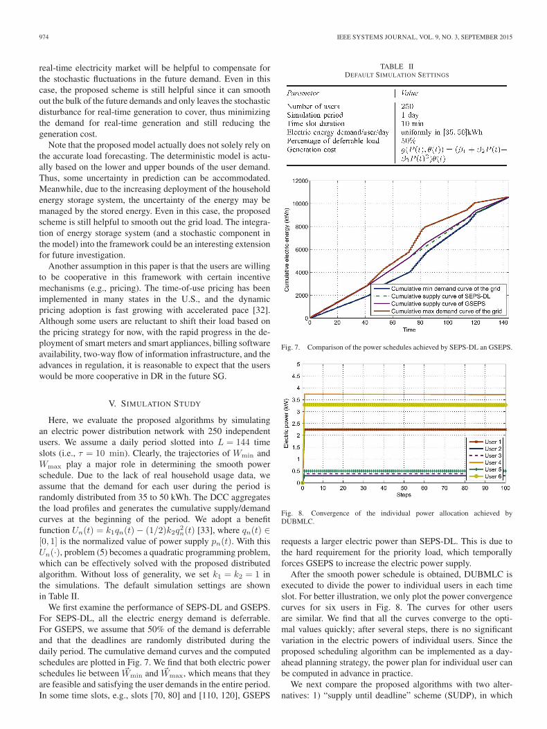
We first examine the performance of SEPS-DL and GSEPS.For SEPS-DL, all the electric energy demand is deferrable.For GSEPS, we assume that 50% of the demand is deferrableand that the deadlines are randomly distributed during thedaily period. The cumulative demand curves and the computedschedules are plotted in Fig. 7. We find that both electric powerschedules lie between �Wmin and �Wmax, which means that theyare feasible and satisfying the user demands in the entire period.In some time slots, e.g., slots [70, 80] and [110, 120], GSEPS

TABLE IIDEFAULT SIMULATION SETTINGS

Fig. 7. Comparison of the power schedules achieved by SEPS-DL an GSEPS.

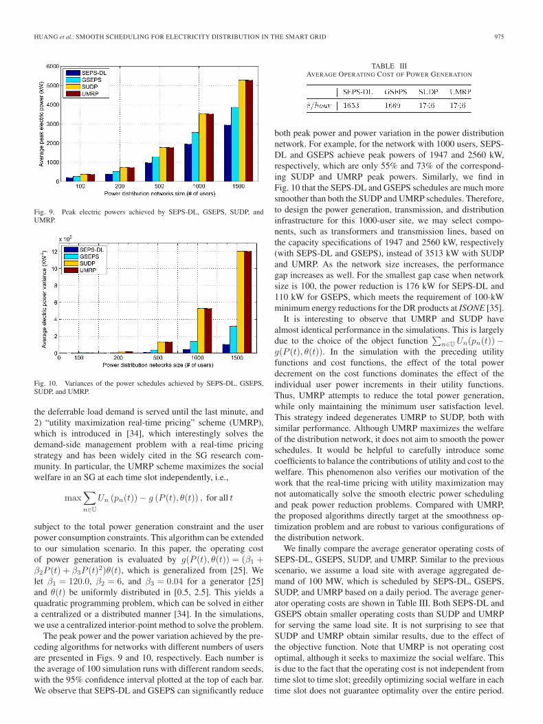
Fig. 8. Convergence of the individual power allocation achieved byDUBMLC.

requests a larger electric power than SEPS-DL. This is due tothe hard requirement for the priority load, which temporallyforces GSEPS to increase the electric power supply.

After the smooth power schedule is obtained, DUBMLC isexecuted to divide the power to individual users in each timeslot. For better illustration, we only plot the power convergencecurves for six users in Fig. 8. The curves for other usersare similar. We find that all the curves converge to the opti-mal values quickly; after several steps, there is no significantvariation in the electric powers of individual users. Since theproposed scheduling algorithm can be implemented as a day-ahead planning strategy, the power plan for individual user canbe computed in advance in practice.

We next compare the proposed algorithms with two alter-natives: 1) “supply until deadline” scheme (SUDP), in which


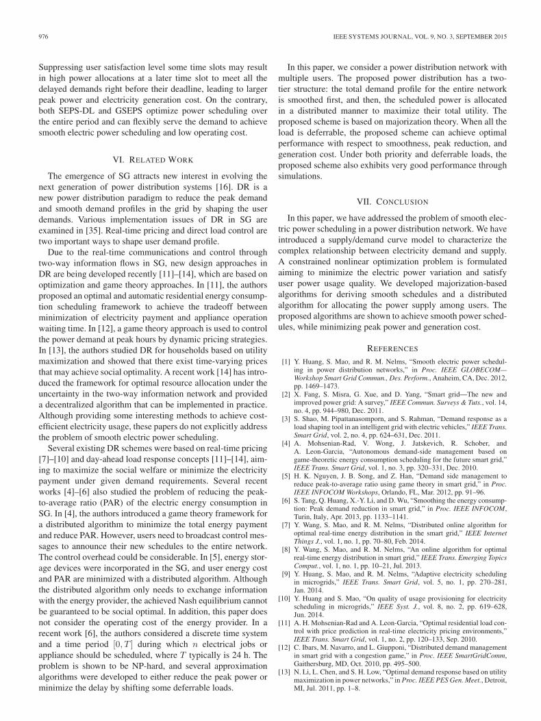
Fig. 9. Peak electric powers achieved by SEPS-DL, GSEPS, SUDP, andUMRP.

Fig. 10. Variances of the power schedules achieved by SEPS-DL, GSEPS,SUDP, and UMRP.

the deferrable load demand is served until the last minute, and2) “utility maximization real-time pricing” scheme (UMRP),which is introduced in [34], which interestingly solves thedemand-side management problem with a real-time pricingstrategy and has been widely cited in the SG research com-munity. In particular, the UMRP scheme maximizes the socialwelfare in an SG at each time slot independently, i.e.,

max∑n∈U

Un (pn(t))− g (P (t), θ(t)) , for all t

subject to the total power generation constraint and the userpower consumption constraints. This algorithm can be extendedto our simulation scenario. In this paper, the operating costof power generation is evaluated by g(P (t), θ(t)) = (β1 +β2P (t) + β3P (t)2)θ(t), which is generalized from [25]. Welet β1 = 120.0, β2 = 6, and β3 = 0.04 for a generator [25]and θ(t) be uniformly distributed in [0.5, 2.5]. This yields aquadratic programming problem, which can be solved in eithera centralized or a distributed manner [34]. In the simulations,we use a centralized interior-point method to solve the problem.

The peak power and the power variation achieved by the pre-ceding algorithms for networks with different numbers of usersare presented in Figs. 9 and 10, respectively. Each number isthe average of 100 simulation runs with different random seeds,with the 95% confidence interval plotted at the top of each bar.We observe that SEPS-DL and GSEPS can significantly reduce

TABLE IIIAVERAGE OPERATING COST OF POWER GENERATION

both peak power and power variation in the power distributionnetwork. For example, for the network with 1000 users, SEPS-DL and GSEPS achieve peak powers of 1947 and 2560 kW,respectively, which are only 55% and 73% of the correspond-ing SUDP and UMRP peak powers. Similarly, we find inFig. 10 that the SEPS-DL and GSEPS schedules are much moresmoother than both the SUDP and UMRP schedules. Therefore,to design the power generation, transmission, and distributioninfrastructure for this 1000-user site, we may select compo-nents, such as transformers and transmission lines, based onthe capacity specifications of 1947 and 2560 kW, respectively(with SEPS-DL and GSEPS), instead of 3513 kW with SUDPand UMRP. As the network size increases, the performancegap increases as well. For the smallest gap case when networksize is 100, the power reduction is 176 kW for SEPS-DL and110 kW for GSEPS, which meets the requirement of 100-kWminimum energy reductions for the DR products at ISONE [35].

It is interesting to observe that UMRP and SUDP havealmost identical performance in the simulations. This is largelydue to the choice of the object function

∑n∈U Un(pn(t))−

g(P (t), θ(t)). In the simulation with the preceding utilityfunctions and cost functions, the effect of the total powerdecrement on the cost functions dominates the effect of theindividual user power increments in their utility functions.Thus, UMRP attempts to reduce the total power generation,while only maintaining the minimum user satisfaction level.This strategy indeed degenerates UMRP to SUDP, both withsimilar performance. Although UMRP maximizes the welfareof the distribution network, it does not aim to smooth the powerschedules. It would be helpful to carefully introduce somecoefficients to balance the contributions of utility and cost to thewelfare. This phenomenon also verifies our motivation of thework that the real-time pricing with utility maximization maynot automatically solve the smooth electric power schedulingand peak power reduction problems. Compared with UMRP,the proposed algorithms directly target at the smoothness op-timization problem and are robust to various configurations ofthe distribution network.

We finally compare the average generator operating costs ofSEPS-DL, GSEPS, SUDP, and UMRP. Similar to the previousscenario, we assume a load site with average aggregated de-mand of 100 MW, which is scheduled by SEPS-DL, GSEPS,SUDP, and UMRP based on a daily period. The average gener-ator operating costs are shown in Table III. Both SEPS-DL andGSEPS obtain smaller operating costs than SUDP and UMRPfor serving the same load site. It is not surprising to see thatSUDP and UMRP obtain similar results, due to the effect ofthe objective function. Note that UMRP is not operating costoptimal, although it seeks to maximize the social welfare. Thisis due to the fact that the operating cost is not independent fromtime slot to time slot; greedily optimizing social welfare in eachtime slot does not guarantee optimality over the entire period.


Suppressing user satisfaction level some time slots may resultin high power allocations at a later time slot to meet all thedelayed demands right before their deadline, leading to largerpeak power and electricity generation cost. On the contrary,both SEPS-DL and GSEPS optimize power scheduling overthe entire period and can flexibly serve the demand to achievesmooth electric power scheduling and low operating cost.

VI. RELATED WORK

The emergence of SG attracts new interest in evolving thenext generation of power distribution systems [16]. DR is anew power distribution paradigm to reduce the peak demandand smooth demand profiles in the grid by shaping the userdemands. Various implementation issues of DR in SG areexamined in [35]. Real-time pricing and direct load control aretwo important ways to shape user demand profile.

Due to the real-time communications and control throughtwo-way information flows in SG, new design approaches inDR are being developed recently [11]–[14], which are based onoptimization and game theory approaches. In [11], the authorsproposed an optimal and automatic residential energy consump-tion scheduling framework to achieve the tradeoff betweenminimization of electricity payment and appliance operationwaiting time. In [12], a game theory approach is used to controlthe power demand at peak hours by dynamic pricing strategies.In [13], the authors studied DR for households based on utilitymaximization and showed that there exist time-varying pricesthat may achieve social optimality. A recent work [14] has intro-duced the framework for optimal resource allocation under theuncertainty in the two-way information network and provideda decentralized algorithm that can be implemented in practice.Although providing some interesting methods to achieve cost-efficient electricity usage, these papers do not explicitly addressthe problem of smooth electric power scheduling.

Several existing DR schemes were based on real-time pricing[7]–[10] and day-ahead load response concepts [11]–[14], aim-ing to maximize the social welfare or minimize the electricitypayment under given demand requirements. Several recentworks [4]–[6] also studied the problem of reducing the peak-to-average ratio (PAR) of the electric energy consumption inSG. In [4], the authors introduced a game theory framework fora distributed algorithm to minimize the total energy paymentand reduce PAR. However, users need to broadcast control mes-sages to announce their new schedules to the entire network.The control overhead could be considerable. In [5], energy stor-age devices were incorporated in the SG, and user energy costand PAR are minimized with a distributed algorithm. Althoughthe distributed algorithm only needs to exchange informationwith the energy provider, the achieved Nash equilibrium cannotbe guaranteed to be social optimal. In addition, this paper doesnot consider the operating cost of the energy provider. In arecent work [6], the authors considered a discrete time systemand a time period [0, T ] during which n electrical jobs orappliance should be scheduled, where T typically is 24 h. Theproblem is shown to be NP-hard, and several approximationalgorithms were developed to either reduce the peak power orminimize the delay by shifting some deferrable loads.

In this paper, we consider a power distribution network withmultiple users. The proposed power distribution has a two-tier structure: the total demand profile for the entire networkis smoothed first, and then, the scheduled power is allocatedin a distributed manner to maximize their total utility. Theproposed scheme is based on majorization theory. When all theload is deferrable, the proposed scheme can achieve optimalperformance with respect to smoothness, peak reduction, andgeneration cost. Under both priority and deferrable loads, theproposed scheme also exhibits very good performance throughsimulations.

VII. CONCLUSION

In this paper, we have addressed the problem of smooth elec-tric power scheduling in a power distribution network. We haveintroduced a supply/demand curve model to characterize thecomplex relationship between electricity demand and supply.A constrained nonlinear optimization problem is formulatedaiming to minimize the electric power variation and satisfyuser power usage quality. We developed majorization-basedalgorithms for deriving smooth schedules and a distributedalgorithm for allocating the power supply among users. Theproposed algorithms are shown to achieve smooth power sched-ules, while minimizing peak power and generation cost.

REFERENCES

[1] Y. Huang, S. Mao, and R. M. Nelms, “Smooth electric power schedul-ing in power distribution networks,” in Proc. IEEE GLOBECOM—Workshop Smart Grid Commun., Des. Perform., Anaheim, CA, Dec. 2012,pp. 1469–1473.

[2] X. Fang, S. Misra, G. Xue, and D. Yang, “Smart grid—The new andimproved power grid: A survey,” IEEE Commun. Surveys & Tuts., vol. 14,no. 4, pp. 944–980, Dec. 2011.

[3] S. Shao, M. Pipattanasomporn, and S. Rahman, “Demand response as aload shaping tool in an intelligent grid with electric vehicles,” IEEE Trans.Smart Grid, vol. 2, no. 4, pp. 624–631, Dec. 2011.

[4] A. Mohsenian-Rad, V. Wong, J. Jatskevich, R. Schober, andA. Leon-Garcia, “Autonomous demand-side management based ongame-theoretic energy consumption scheduling for the future smart grid,”IEEE Trans. Smart Grid, vol. 1, no. 3, pp. 320–331, Dec. 2010.

[5] H. K. Nguyen, J. B. Song, and Z. Han, “Demand side management toreduce peak-to-average ratio using game theory in smart grid,” in Proc.IEEE INFOCOM Workshops, Orlando, FL, Mar. 2012, pp. 91–96.

[6] S. Tang, Q. Huang, X.-Y. Li, and D. Wu, “Smoothing the energy consump-tion: Peak demand reduction in smart grid,” in Proc. IEEE INFOCOM,Turin, Italy, Apr. 2013, pp. 1133–1141.

[7] Y. Wang, S. Mao, and R. M. Nelms, “Distributed online algorithm foroptimal real-time energy distribution in the smart grid,” IEEE InternetThings J., vol. 1, no. 1, pp. 70–80, Feb. 2014.

[8] Y. Wang, S. Mao, and R. M. Nelms, “An online algorithm for optimalreal-time energy distribution in smart grid,” IEEE Trans. Emerging TopicsComput., vol. 1, no. 1, pp. 10–21, Jul. 2013.

[9] Y. Huang, S. Mao, and R. M. Nelms, “Adaptive electricity schedulingin microgrids,” IEEE Trans. Smart Grid, vol. 5, no. 1, pp. 270–281,Jan. 2014.

[10] Y. Huang and S. Mao, “On quality of usage provisioning for electricityscheduling in microgrids,” IEEE Syst. J., vol. 8, no. 2, pp. 619–628,Jun. 2014.

[11] A. H. Mohsenian-Rad and A. Leon-Garcia, “Optimal residential load con-trol with price prediction in real-time electricity pricing environments,”IEEE Trans. Smart Grid, vol. 1, no. 2, pp. 120–133, Sep. 2010.

[12] C. Ibars, M. Navarro, and L. Giupponi, “Distributed demand managementin smart grid with a congestion game,” in Proc. IEEE SmartGridComm,Gaithersburg, MD, Oct. 2010, pp. 495–500.

[13] N. Li, L. Chen, and S. H. Low, “Optimal demand response based on utilitymaximization in power networks,” in Proc. IEEE PES Gen. Meet., Detroit,MI, Jul. 2011, pp. 1–8.


[14] M. G. Kallitsis, G. Michailidis, and M. Devetsikiotis, “Optimal power al-location under communication network externalities,” IEEE Trans. SmartGrid, vol. 3, no. 1, pp. 162–173, Mar. 2012.

[15] M. LeMay, R. Nelli, G. Gross, and C. A. Gunter, “An integrated architec-ture for demand response communications and control,” in Proc. HICSS,Washington, DC, 2008, pp. 174–183.

[16] G. T. Heydt, “The next generation of power distribution systems,” IEEETrans. Smart Grid, vol. 1, no. 3, pp. 225–235, Dec. 2010.

[17] J. Kumagai, “Virtual power plants, real power,” IEEE Spectr., vol. 49,no. 3, pp. 13–14, Mar. 2012.

[18] H. Farhangi, “The path of the smart grid,” IEEE Power Energy Mag.,vol. 8, no. 1, pp. 18–28, Jan./Feb. 2010.

[19] J. Medina, N. Muller, and I. Roytelman, “Demand response and distribu-tion grid operations: Opportunities and challenges,” IEEE Trans. SmartGrid, vol. 1, no. 2, pp. 193–198, Sep. 2010.

[20] A. W. Marshall and I. Olkin, Inequalities: Theory of Majorization and ItsApplications. New York, NY, USA: Academic, 1979.

[21] J. Salehi, Z.-L. Zhang, J. Kurose, and D. Towsley, “Supporting storedvideo: Reducing rate variability and end-to-end resource requirementsthrough optimal smoothing,” IEEE/ACM Trans. Netw., vol. 6, no. 4,pp. 397–410, Aug. 1998.

[22] E. Jorswieck and H. Boche, “Optimal transmission strategies and impactof correlation in multiantenna systems with different types of channel stateinformation,” IEEE Trans. Signal Process., vol. 52, no. 12, pp. 3440–3453, Dec. 2004.

[23] A. Papavasiliou and S. S. Oren, “Supplying renewable energy to de-ferrable loads: Algorithms and economic analysis,” in Proc. IEEE Power& Energy Soc. Gen. Meet., Jul. 2010, pp. 1–8.

[24] B. C. Arnold, Majorization and the Lorenz Order: A Brief Introduction.New York, NY, USA: Springer-Verlag, 1987.

[25] A. J. Wood and B. F. Wollenberg, Power Generation, Operation, andControl. New York, NY, USA: Wiley, 1984.

[26] D. P. Palomar and M. Chiang, “A tutorial on decomposition methodsfor network utility maximization,” IEEE J. Sel. Areas Commun., vol. 24,no. 8, pp. 1439–1451, Aug. 2006.

[27] D. Bertsekas, Nonlinear Programming. Belmont, MA, USA: AthenaScientific, 1995.

[28] M. Ghofrani, M. Hassanzadeh, M. Etezadi-Amoli, and M. Fadali, “Smartmeter based short-term load forecasting for residential customers,” inProc. NAPS, Boston, MA, Aug. 2011, pp. 1–5.

[29] M. Chaouch, “Clustering-based improvement of nonparametric functionaltime series forecasting: Application to intra-day household-level loadcurves,” IEEE Trans. Smart Grid, vol. 5, no. 1, pp. 411–419, Jan. 2014.

[30] B. Stephen, F. Isleifsson, S. Galloway, G. Burt, and H. Bindner, “Onlineamr domestic load profile characteristic change monitor to support ancil-lary demand services,” IEEE Trans. Smart Grid, vol. 5, no. 2, pp. 888–895, Mar. 2014.

[31] B. Walsh, “Breakthrough: Smart Power-Data-crunching algorithms, notsolar panels, are the new darlings of clean tech,” Time Mag., p. 10,Apr. 8, 2013.

[32] Energy.gov, “Energy Policy Act of 2005,” Public Law 10958,109th Congress. [Online]. Available: http://energy.gov/eere/femp/energy-policy-act-2005

[33] M. Fahrioglu and F. L. Alvarado, “Designing incentive compatible con-tracts for effective demand management,” IEEE Trans. Power Syst.,vol. 15, no. 4, pp. 1255–1260, Nov. 2000.

[34] P. Samadi, A. Mohsenian-Rad, R. Schober, V. Wong, and J. Jatskevich,“Optimal real-time pricing algorithm based on utility maximization forsmart grid,” in IEEE SmartGridComm, Oct. 2010, pp. 415–420.

[35] F. Rahimi and A. Ipakchi, “Demand response as a market resource underthe smart grid paradigm,” IEEE Trans. Smart Grid, vol. 1, no. 1, pp. 82–88, Jun. 2010.

Yingsong Huang (S’12) received the B.S. degree inautomation and the M.S. degrees in control theoryand control engineering and from Chongqing Uni-versity, Chongqing, China, and the Ph.D. degree inelectrical and computer engineering from AuburnUniversity, Auburn, AL, USA, in 2013.

From July 2003 to July 2007, he was a Se-nior Research and Development Engineer and aVice-Supervisor with Advantech Corporation, Ltd.,Beijing and Taipei, China. He is currently a Memberof Technical Staff with NetApp, Inc., Pittsburgh, PA,

USA. His research interests include modeling, control and optimization inmicrogrids, smart grid, and computer networks.

Shiwen Mao (S’99–M’04–SM’09) received thePh.D. degree in electrical and computer engineeringfrom Polytechnic University, Brooklyn, NY, USA.

He is currently the McWane Associate Professorin the Electrical and Computer Engineering De-partment, Auburn University, Auburn, AL, USA.His research interests include wireless networks andmultimedia communications, with current focus oncognitive radio, small cells, 60-GHz millimeter-wave networks, free-space optical networks, andsmart grid.

Prof. Mao is a Distinguished Lecturer of the IEEE Vehicular TechnologySociety in the Class of 2014. He is on the Editorial Board of the IEEETRANSACTIONS ON WIRELESS COMMUNICATIONS, the IEEE Internet ofThings Journal, and the IEEE Communications Surveys and Tutorials, amongothers. He was a recipient of the 2013 IEEE ComSoc MMTC OutstandingLeadership Award and the NSF CAREER Award in 2010. He was a corecipientof the IEEE ICC 2013 Best Paper Award and The 2004 IEEE CommunicationsSociety Leonard G. Abraham Prize in the field of communications systems.

R. M. Nelms (F’04) received the B.E.E. and M.S.degrees from Auburn University, Auburn, AL, USA,in 1980 and 1982, respectively, and the Ph.D. degreefrom Virginia Polytechnic Institute and State Univer-sity, Blacksburg, VA, USA, in 1987, all in electricalengineering.

He is currently a Professor and the Chair of theElectrical and Computer Engineering Departmentwith Auburn University. His research interests arein power electronics, power systems, and electricmachinery.

Prof. Nelms was named an IEEE Fellow “for technical leadership andcontributions to applied power electronics.” He is a Registered ProfessionalEngineer in Alabama.

smooth scheduling for electricity distribution in the …szm0001/papers/isj_2045.final.pdfhuanget...

Documents