snr estimation using extended kalman filter...
TRANSCRIPT

i
SNR ESTIMATION USING EXTENDED KALMAN FILTER TECHNIQUE FOR
ORTHOGONAL FREQUENCY DIVISION MULTIPLEXING (OFDM) SYSTEM
SYLVIA ONG AI LING
A thesis submitted in
fulfillment of the requirement for the award of the
Degree of Master of Electrical Engineering
Faculty of Electrical and Electronic Engineering
Universiti Tun Hussein Onn Malaysia
JULY 2012
iv
ABSTRACT
Signal to Noise Ratio (SNR) estimation of a received signal is an important and
essential information for Orthogonal Frequency Division Multiplexing (OFDM)
system. This is because in OFDM system, robustness in frequency selective channels
can be achieved using adaptable transmission parameters. Therefore, to reckon these
parameters, knowledge of SNR estimates obtained by channel state information is
required for optimal performance. The performance of SNR estimation algorithm is
contingent on channel estimates obtained through channel estimation schemes. In
this project, two estimators which are Least Square (LS) and Minimum Mean Square
Error (MMSE) estimators are simulated and analyzed. From the result obtained, LS
shows better performance than MMSE in terms of Symbol Error Rate (SER) and
Mean Square Error (MSE) via computer simulation. With different number of sub
carriers implemented for the system model, 16, 32, 64, the result apparently shows
that the SER curve of the estimator with the highest number of sub carriers, 64 is
significantly lower compare with the other estimators with sub carriers of 16 and 32.
Therefore, a system model which contribute to 64 sub carriers are implemented.
However, in case of wireless channels, they possess non linearity where the LS and
MMSE, linear estimators yield inefficient results. Therefore, to improve the SNR
estimation, an efficient non linear Extended Kalman Filter (EKF) estimation, is
implemented into the OFDM system. The EKF estimator outperforms the LS and
MMSE estimators in terms of SER and MSE for AWGN channel. The beauty of the
estimation is that it can estimate the past, present and future.
v
ABSTRAK
Anggaran nisbah isyarat kepada hingar (SNR) yang diterima adalah maklumat yang
penting dan berguna untuk sistem Pemultipleksan Pembahagian Frekuensi ortogon
(OFDM). Ini adalah kerana dalam sistem OFDM, keteguhan dalam saluran memilih
frekuensi boleh dicapai dengan menggunakan parameter penghantaran yang sesuai.
Oleh itu, untuk mendapatkan maklumat parameter ini, pengetahuan tentang
penganggaran SNR diperolehi melalui saluran maklumat yang diperlukan untuk
prestasi optimum. Prestasi algoritma anggaran SNR adalah bergantung kepada
anggaran saluran yang diperolehi melalui skim anggaran saluran. Dua teknik
anggaran yang telah dikaji oleh penyelidik lain telah dianalisis, Least Square (LS)
dan Minimum Mean Square Error (MMSE). Daripada keputusan kajian ini, LS
menunjukkan prestasi yang lebih baik daripada MMSE dari segi Symbol Error Rate
(SER) dan Mean Square Error (MSE) melalui simulasi komputer. Melalui jumlah
pembawa sub yang berbeza bagi model sistem, 16, 32, 64, hasilnya jelas
menunjukkan bahawa keluk SER penganggar dengan bilangan pembawa sub
tertinggi, 64 adalah jauh lebih rendah berbanding dengan penganggar lain dengan
pembawa sub 16 dan 32. Oleh itu, satu model sistem yang menyumbang kepada 64
pembawa sub dikaji. Walau bagaimanapun, bagi kes saluran tanpa wayar, yang
bukan linear, LS dan MMSE, penganggar linear menghasilkan keputusan yang tidak
cekap. Bagi meningkatkan anggaran SNR dengan tepat, Extended Kalman Filter
(EKF), dilaksanakan dalam sistem OFDM. Melalui simulasi, kaedah EKF melebihi
prestasi LS dan MMSE dari segi SER dan MSE untuk saluran Additive White
Gaussian Noise (AWGN). Kelebihan anggaran adalah bahawa ia boleh
menganggarkan element lepas, semasa dan depan.

vi
CONTENTS
TITLE i
DECLARATION ii
ACKNOWLEDGEMENT v
ABSTRACT vi
CONTENTS viii
LIST OF TABLE x
LIST OF FIGURES xi
LIST OF ABBREVIATIONS xiii
CHAPTER 1 INTRODUCTION
1.1 Introduction 1
1.2 Problem of Statement 2
1.3 Project Objectives 3
1.4 Scopes 3
1.5 Outline 4
CHAPTER 2 SNR ESTIMATION : A REVIEW
2.1 Introduction 6
2.1.1 System Model 6
2.2 SNR estimation algorithms 8
2.2.1 Minimum Mean Square Error (MMSE)
Estimation 13
2.2.2 Least Square (LS) Estimation 14
2.2.3 Kalman Filter Estimation 15
CHAPTER 3 AN OVERVIEW OF OFDM
3.1 Introduction 17
3.2 Overview of OFDM 17

vii
3.2.1 Basic Principles of OFDM System 19
3.2.2 Serial to Parallel Conversion 21
3.2.3 Modulation 21
3.2.4 IFFT Operation 21
3.2.5 Cyclic Prefix Insertion 22
3.2.6 Parallel to Serial Conversion 23
3.3 OFDM System Sub-Carrier Signal 23
3.4 OFDM Advantages and Disadvantages 25
CHAPTER 4 METHODOLOGY : MODEL SIMULATION
4.1 Introduction 27
4.2 Simulink Implementation 27
4.3 Project Model Simulation 29
4.3.1 Random Data Source 30
4.3.2 Forward Error Correction 31
4.3.2.1 Reed Solomon (RS) Encoder 31
4.3.2.2 Convolution Encoder / Viterbi
Decoder 32
4.3.2.3 Interleaver / Deinterleaver 34
4.3.2.4 Modulation / Demodulation 35
4.3.3 OFDM Transmitter 35
4.3.4 OFDM Receiver 37
4.3.5 SNR Estimation using Extended
Kalman Filter (EKF) Estimation 38
CHAPTER 5 RESULTS AND DISCUSSION
5.1 Introduction 44
5.2 Performance Results and Analysis 44
5.2.1 OFDM System Simulation 44
5.2.2 SNR Estimation Simulation 47
5.2.3 EKF Elements 55
CHAPTER 6 SUMMARY
6.1 Introduction 59
6.2 Conclusion 59
6.3 Future Works 60
REFERENCES 61

viii
LIST OF TABLES
1.1 Parameter of OFDM systems 4
2.1 Comparison of previous works by other researchers. 11
2.2 Discrete Kalman filter time and measurement update
equations. 15
4.1 Simulink toolbox parameters 28
ix
LIST OF FIGURES
2.1 OFDM frame structure 6
2.2 Estimation methods 8
2.3 Gaussian Channels 12
2.4 The Kalman filter cycle 15
3.1 The frequency division for OFDM systems 18
3.2 OFDM system 19
3.3 Illustration of the Cyclic Prefix insertion in an OFDM
Symbol 22
3.4 OFDM system sub-carrier signal 23
3.5 OFDM symbol structure 24
4.1 Project Implementation 28
4.2 Project Model 29
4.3 Bernoulli Binary Generator 30
4.4 Reed-Solomon Encoder 31
4.5 (a) Convolutional Encoder (b) Viterbi Decoder 32
4.6 Convolutional Encoder 33
4.7 Interleaver 34
4.8 OFDM Transmitter 36
4.9 OFDM Receiver 37
4.10 Proposed SNR estimation using EFK 38
4.11 Data flow in EKF 41
4.12 SNR estimation 42
5.1 Transmitted and Received QPSK Signal
Constellation Mapper through AWGN channel 46
5.2 Spectrum plot of signal 47

x
5.3 Comparison between MMSE and LS estimator
in terms of MSE 47
5.4 Comparison between MMSE and LS estimator
in terms of SER 49
5.5 SERs performance of the LS and MMSE estimators
with different number of sub carriers 50
5.6 Comparison of MMS/LS/EKF estimators in terms
of SER 52
5.7 Comparison of MMS/LS/EKF estimators in terms
of MSE in AWGN channel 52
5.8 Comparison between estimated versus actual
SNR with proposed method 53
5.9 Comparison of MMS/LS/EKF estimators in terms
of MSE in Rayleigh 54
5.10 Comparison of state with a priori, a posterior
elements and exact values. 55
5.11 Comparison between the actual a priori and a
posteriori error 56
5.12 Comparison between a priori and a posterior
Covariance 56
5.13 Kalman gain 57
xi
LIST OF ABBREVIATIONS
ADSL Asynchronous Digital Subscriber Line
AWGN Additive White Gaussian Noise
BPSK Binary Phase Shift Keying
CP Cyclic Prefix
CTC Convolutional Turbo Coding
DA Data Aided
DAB Digital Audio Broadcasting
DC Direct Current
DFT Discrete Fourier Transform
DSP Digital Signal Processor/Processing
DVB-T Terrestrial Video Broadcasting
EKF Extended Kalman Filtering
FDM Frequency Division Multiplexing
FEC Forward Error Correction
FFT Fast Fourier Transform
HDSL High bit-rate Digital Subscriber Line Systems
IFFT Inverse Fast Fourier Transform
ICI Inter Carrier Interference
ISI Inter Symbol Interference
KF Kalman Filter
LS Least Square
M2 M4 Second- and Fourth- Order Moments
MIMO Multiple Input Multiple Output
ML Maximum Likelihood
MSE Mean Square Error
MMSE Minimum Mean Square Error
xii
NDA Non Data Aided
NMSE Normalised Mean Square Error
NLOS Non Line-Of-Sight
OFDM Orthogonal Frequency Division Multiplexing
PAPR Peak-to-Average Power Ratio
PRBS Pseudorandom Binary Sequence
PSK Pulse Shift Keying
QPSK Quardrature Pulse Shift Keying
QAM Quardrature Amplitude Modulation
RS Reed Solomon
SER Symbol Error Rate
SFN Single Frequency Network
SNR Signal to Noise Ratio
SSME Split Symbol Moments Estimator
SVR Signal to Variance Ratio
VLSI Very Large Scale Integrated Circuits
WiMAX Worldwide Interoperability for Microwave Access

1
CHAPTER 1
INTRODUCTION
1.1 Introduction
Orthogonal Frequency Division Multiplexing (OFDM) have been invented for more
than 40 years ago and is implemented in wide variety of applications in digital
transmission system. OFDM has proven to be useful in frequency-selective channels
to achieve high data rates and has been abundantly proposed for high-data rate
transmission system. In the past, OFDM applications have been scarce because of the
complexity involved in practical implementation. Recent advances in technology
such as Very Large Scale Integrated Circuits (VLSI) and Digital Signal Processors
(DSPs) have enabled the cost-effective and practical implementation of the Discrete
Fourier Transform (DFT) / Inverse Fast Fourier Transform (IFFT) via the Fast
Fourier Transform (FFT) / Inverse Fast Fourier Transform (IFFT) operation on a
single chip for Digital Audio Broadcasting standard (DAB) and TerrestrialVideo
Broadcasting (DVB-T) systems. OFDM is also employed for fixed wireline
applications such as Asynchronous Digital Subscriber Line (ADSL) and High bit-
rate Digital Subscriber Line Systems (HDSL). Standard IEEE 802.11a/g, wireless
broadband access standards IEEE 802.16a (WiMAX), and the core technique for
fourth-generation (4G) wireless mobile communications were also incorporate
OFDM.
OFDM is a multicarrier modulation scheme with excellent robustness in
multi-path environments by dividing the high-data rate channel over multiple and
very narrow parallel channels,where each is modulated on a different subcarriers.
The data rate in the individual carriers are reduced significantly, while still

2
maintaining overall throughput. To ensure that sub-carriers do not interfere with each
other in frequency domain, subchannels orthogonalization is performed using the fast
Fourier transform (FFT). Hence the inter symbol interference (ISI) due to multipath
delay spread is reduced. Pilot symbols are used to estimate the complex gains of the
parallel subchannels. Moreover, cyclic prefix added at the transmitter helps to reduce
the receiver complexity for FFT processing. This mechanism facilitates the design of
single frequency networks (SFNs). However, reliable communication in wireless
system, becomes a difficult task as the transmitted data is not only corrupted by
Additive White Gaussian Noise (AWGN), but also suffers from ISI as well as
interference or colored noise from other users. Color of the noise is caused by its
uneven spectral variation. Accurate Signal to Noise Ratio (SNR) estimation at
receiver is important to modify the transmission parameter for channel quality
control.
SNR can be used to characterize the link quality. It is an important factor in a
receiver performance on how well the recovering of the information-carrying signal
from its corrupted version and hence how reliably information can be communicated.
SNR can be defined in its simplest form as ratio of signal power to noise power.
Generally, there are two categories of knowledge-based SNR estimators, Data-aided
(DA) and Non Data-Aided (NDA). DA estimators are based on the knowledge of the
transmitted data, in which the bandwidth efficiency is reduced, while NDA estimates
SNR from an unknown information.
1.2 Problem of Statement
Modern wireless communication systems has come a long way since 1897. It has the
ability transfer of information between two or more points without the need of a
fixed cable connection. Wireless communication systems is used to meets many
needs, from the traditional voice application to multimedia, pushing the needs for
higher data rate and faster transmission speed. As the demand of data rate and
transmission speed increases in recent years, the noise and ISI also increases due to
multipath fadings.
Multipath signals due to different delays is caused by reflections of the signal
and different propagation paths between the transmitters and receivers. These
reflected components add up either constructively or destructively at the receiver,
3
and the resulting effect is known as frequency selective fading. During the
propagation of the signal through the channel, the signal also suffers rapid fluctuation
in amplitude and phase. It is very important to combat the effects of the fadings
because the amount of fading is directly related to the throughput of the system. A
multicarrier modulation, OFDM is a popular and powerful method to combat the
frequency selective channels. A fixed-mode transceivers cannot perform effectively
over a dispersive channel, as severe SNR fluctuations occurs. It is this drawback that
been a motivating factor for research on adaptive transceivers. Adaptation in
conjunction with OFDM, is a powerful method to mitigate the frequency selective
fading and utilize the maximum available capacity of the time varying channel. The
performance of adaptive OFDM systems depends on the effectiveness of techniques
used in channel quality estimation, particularly SNR estimation. In order to achieve
improvement by exploiting frequency selective channels in designing OFDM system,
accurate and exact SNR estimation is requisite. There are many other applications
that can exploit SNR information, such like channel estimation through interpolation
and optimal soft information generation for high performance decoding algorithms.
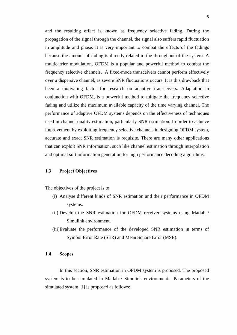
1.3 Project Objectives
The objectives of the project is to:
(i) Analyse different kinds of SNR estimation and their performance in OFDM
systems.
(ii) Develop the SNR estimation for OFDM receiver systems using Matlab /
Simulink environment.
(iii)Evaluate the performance of the developed SNR estimation in terms of
Symbol Error Rate (SER) and Mean Square Error (MSE).
1.4 Scopes
In this section, SNR estimation in OFDM system is proposed. The proposed
system is to be simulated in Matlab / Simulink environment. Parameters of the
simulated system [1] is proposed as follows:

4
Table 1.1 Parameter of OFDM systems
Parameter Values
Channel Bandwidth (MHz) 5
Sampling Frequency (fp, MHz) 5.6
IFFT Size 512
Number of sub carriers 128
Number of sub bands 32
Number of sub carriers per sub band 16
Frame size 6
SNR 1-35dB
Modulation schemes MQAM
Carrier Frequency (GHz) 2
Subcarrier Frequency Spacing (kHz) 10.94
Useful Symbol Time (Tb = 1/f, μs) 91.4
Guard Time Duration (Tg = Tb/8, μs) 11.4
OFDM Symbol duration (Ts = Tb + Tg , μs) 102.9
Number of OFDM Symbols (5 ms Frame) 48
1.5 Outline
This thesis comprises of six chapters.
Chapter 1:
This chapter introduces the project overview, which consists of OFDM and SNR
estimation introduction, problem of statement, objectives, scope and outline.
Chapter 2:
This chapter presents a detailed description of OFDM systems, which consists of the
building blocks, operation, and signal processing.

5
Chapter 3:
This chapter outlines a brief overview of works done by previous researchers which
describes the enabling techniques that facilitate efficient SNR estimation. This
chapter also discuss in details on the consideration of wireless channel models, with
white and Gaussian distributed interfering noise, AWGN and fadings.
Chapter 4:
This chapter presents the MATLAB/SIMULINK project model simulation
discussion. This chapter will also give a brief explanation and description for each
model block.
Chapter 5:
In this chapter, the simulation results on the model performance are illustrated. This
is followed with the simulation result analysis in terms of SER and MSE.
Chapter 6:
This chapter presents the conclusions and topics for further research, of this work.
6
CHAPTER 2
SNR ESTIMATION : A REVIEW
2.1 Introduction
This chapter discuss related research work focusing on SNR estimation algorithms
and channel estimation schemes done by other researchers.
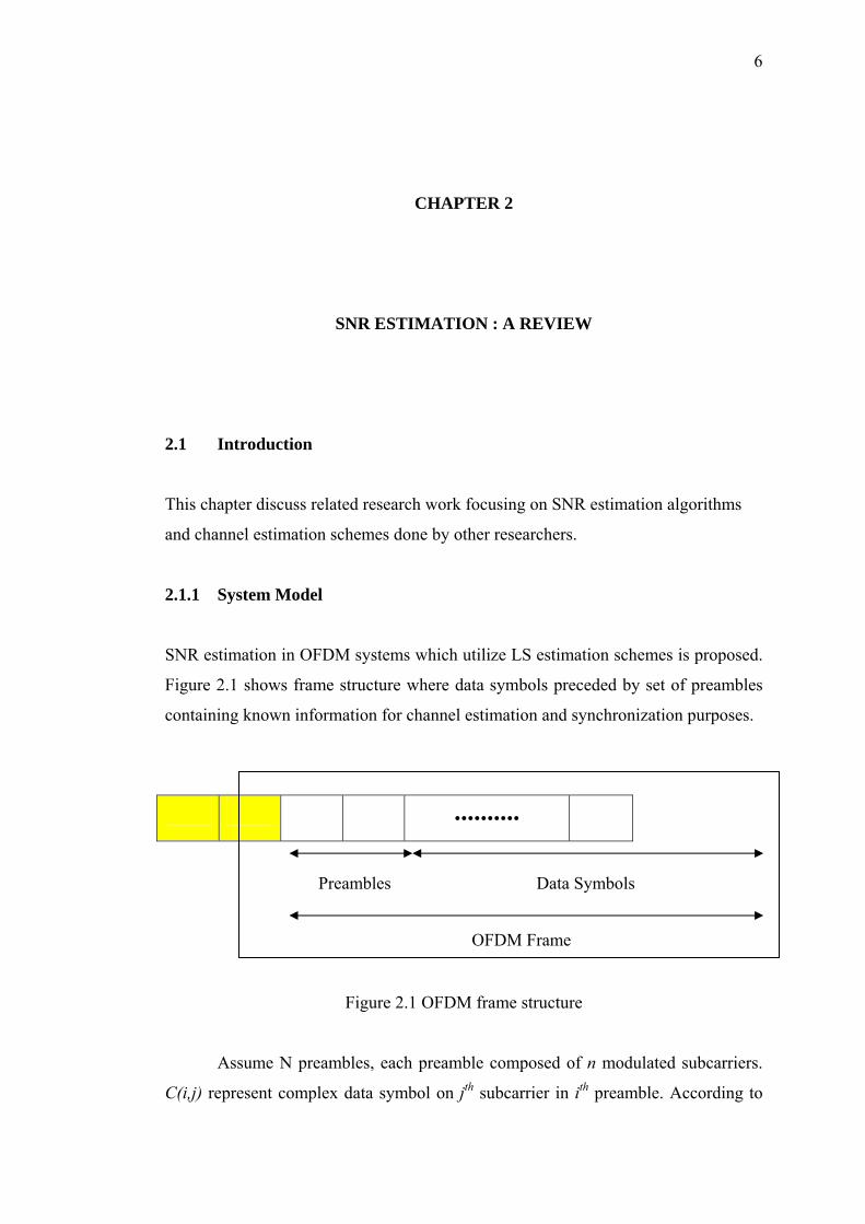
2.1.1 System Model
SNR estimation in OFDM systems which utilize LS estimation schemes is proposed.
Figure 2.1 shows frame structure where data symbols preceded by set of preambles
containing known information for channel estimation and synchronization purposes.
..........
Preambles Data Symbols
OFDM Frame
Figure 2.1 OFDM frame structure
Assume N preambles, each preamble composed of n modulated subcarriers.
C(i,j) represent complex data symbol on jth subcarrier in ith preamble. According to

7
OFDM standards as preambles consist of QPSK modulated subcarriers, assume unit
magnitude modulated subcarrier |C(i,j)|2 = 1. Perfect synchronization is assumed in
frequency domain and the received signal is given as
(2.1)
where S, W are transmitted signal and noise powers respectively, η(i,j) is sampled
complex zero mean AWGN and H(i,j) is channel frequency response expressed as
(2.2)
where L denote the length of Channel Impulse Response (CIR), h(τl + iTs) signify
channel path gain with delay τl in lth path of ith OFDM preamble of duration Ts.
Consider channel to be constant for whole frame assuming that SNR estimation
algorithms are implemented for adaptive transmissions. CIR paths are opted to be
integer multiples of system sampling rate where The
estimates of average SNR and SNR per subcarrier are valid for all data carrying
OFDM symbols.
As shown in [2], the average SNR is given as
(2.3)
The SNR on the jth subcarrier is expressed as
(2.4)

8
2.2 SNR estimation algorithms
SNR has long been used as the standard measure of analog signals quality in noisy
environments. There are various types of SNR estimation methods developed for
OFDM systems usage as shown in Figure 2.2.
Estimation
Bayesian Estimation (Random Parameter)
Classical Estimation (Deterministic
parameter)
Cramer-Rao Lower Bound
Minimum Mean Square Estimation
Least Squares Estimation
Recursive least squares estimation
Kalman Filtering
Autoregressive
Wiener Filtering
Maximum Likelihood Estimation
Minimum Variance Unbiased Estimation
Maximum a Posteriori Estimation
Figure 2.2 Estimation methods
Pauluzzi D.R. [3] present five different SNR estimation techniques for Pulse
Shift Keying (PSK) modulation in an AWGN channel. The algorithms are called
SSME (Split Symbol Moments Estimator), which is valid for Binary Pulse Shift
Keying (BPSK) modulation only, ML (Maximum Likelihood), SNV (Signal to Noise
Variance), M2M4 (Second- and Fourth-Order Moments) and SVR (Signal to

9
Variance Ratio). ML estimator is implemented as NDA and DA estimators where
DA achieves better results at low SNR values. SNV estimator is a special case of ML
estimator which is based on first and second order moments of the sampled output.
Second-and-Fourth-Order Moments (M2M4) estimator shows similar performance as
ML estimator at high SNR values. SVR estimator performs similar to ML at low
SNR values. The performance of the SNR estimator only applies if the transmitter
knows the channel estimates. [3] Pauluzzi D.R. also assumes that in the jth symbol
period, the ith pilot subcarrier is modulated with a complex value a(i,j). The same
pilot signal is assumed to be sent on the same pilot subcarrier in different OFDM
symbol periods, which means a(i,j) = a(i,l) for any i,j and l. Then the complex
baseband system model for the ith pilot subcarrier can be formulated as
(2.5)
where n(i,j) is complex, zero-mean AWGN and h(i,j) is the complex channel factor.
It is assumed that the variance of h(i,j), n(i,j) and a(i,j) are assumed to be normalized
to unity. S is a signal power scale factor, and N is a noise power scale factor. OFDM
converts a multipath channel into a set of parallel time-variant linear channels.
The M2M4 algorithm and Bourmard’s Algorithm [4] does not require the
channel estimates in order to estimate the SNR estimation at the back-end of
receiver. SNR estimation algorithm for 2X2 Multiple Input Multiple Output
(MIMO)-OFDM systems in [5] requires 30 preambles at each transmitting antenna
for noise estimates. The performance of the algorithm deteriorates with faster
channel fading as Doppler frequency increases. This algorithm is based on the
assumption that the channel varies slowly in time as well as frequency. Two
consecutive time-domain channel estimates for any antenna pair are considered
identical. In addition the channel degradation for adjacent OFDM subcarriers is
considered the same. In this technique, SNR estimation is obtained from noise
variance and Least Square (LS) channel estimates. Many of these estimators
estimates at the back-end of the received. Only a few SNR estimations at front-end of
the receiver are proposed. Rana Shahid Manzoor and et. [6] proposed noise power
and SNR estimation autocorrelation-based using only one OFDM preamble at front-
end of the receiver and data-aided linear prediction based SNR estimation for

10
AWGN channel. It is proven that the NMSE performs better result with 1 OFDM
preamble compared to 30 and 50 OFDM preambles by Boumard, S. [4] and Reddy,
S. [7]. It is observed that front-end estimation of SNR is performing excellently and
providing reliable estimation by Rana Shahid Manzoor and et. [6].
Many of these estimators are based on the knowledge of pilot sequence, Data-
Aided (DA) estimation. DA based approaches are widely implemented to estimate
the channel characteristics and to correct the corrupted channel due to multipath
fading. The SNR estimation technique presented by Xiadong, X. [8], data-aided
estimator is based on tracking the delay-subspace using the estimated channel
correlation matrix. This method required M pilot subcarriers to be inserted into every
OFDM symbol. The channel frequency response for each pilot was found when the
received pilot was divided with the original. The correlation matrix R were computed
through eigenvalue decomposition and L, number of paths, was estimated by the
Minimum Descriptive Length technique in [9]. The estimated eigenvalues and
number of paths was then used to compute the SNR. It was shown by simulation
results, that this estimator is able to estimate the true SNR accurately after an
observation interval of about 20 OFDM symbols for various fading channels.
However, in practical wireless system, the assumption that M > L made by M. Wax
[9] may not apply.
DA SNR estimators using training sequence limits system through-out. In
order to overcome DA method limitation, NDA SNR estimator is proposed in [2]
where the technique is targeted towards applications such as cognitive radio. This is
because the terminals need to sense the link quality with all the surrounding networks
in order to find the most suitable link for communication. This method does not
require the receiver to know the pilots’ locations. Instead the cyclostationarity
induced by the cyclic-prefix is used to determine the SNR. They often suffer from
high computation complexity and low convergence speed since they often need a
large amount of receiving data to obtain some statistical information which is the
cyclostationarity induced by the cyclic prefix. Blind channel estimation methods are
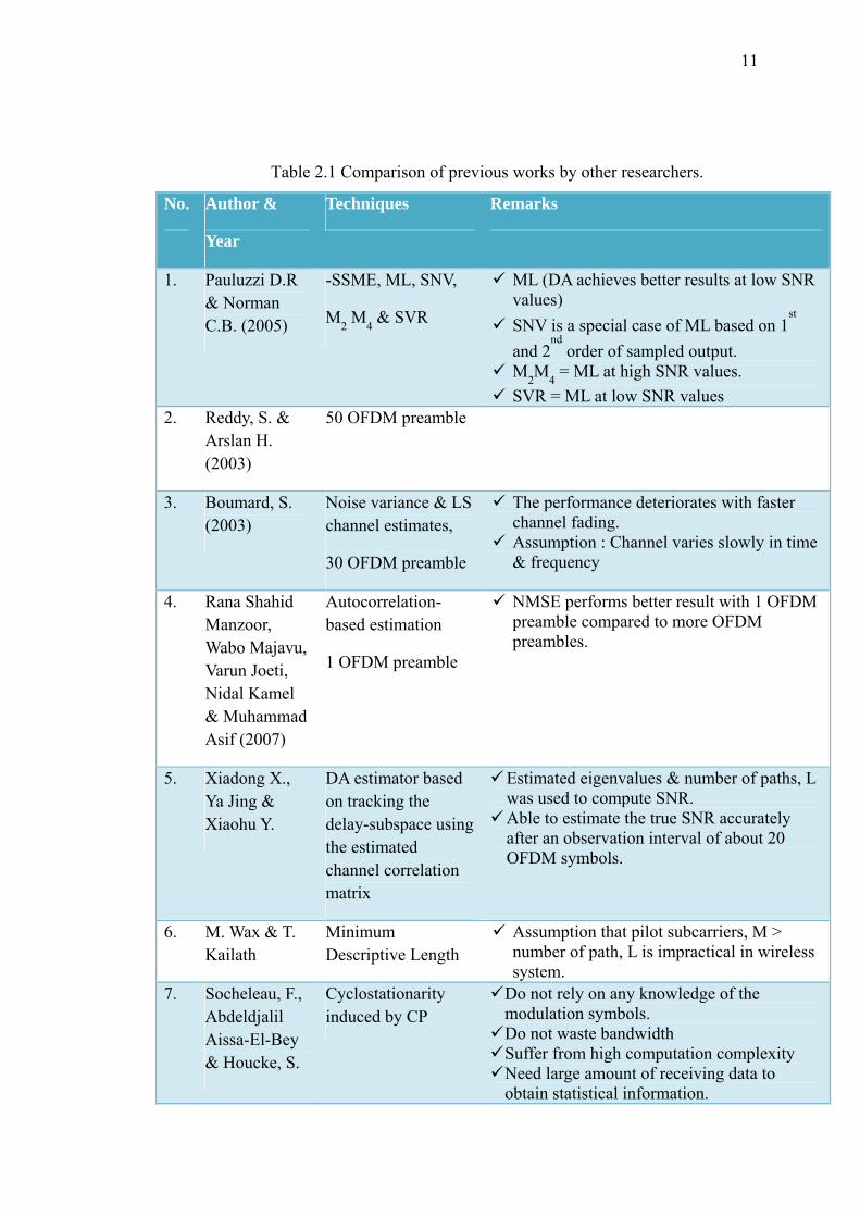
not suitable for applications with fast varying fading channels. Table 2.1 shows the
summary of the previous works by other researchers.
11
Table 2.1 Comparison of previous works by other researchers.
No. Author &
Year
Techniques Remarks
1. Pauluzzi D.R & Norman C.B. (2005)
-SSME, ML, SNV,
M2 M4 & SVR
ML (DA achieves better results at low SNR values)
SNV is a special case of ML based on 1st
and 2nd
order of sampled output. M2M4 = ML at high SNR values. SVR = ML at low SNR values
2. Reddy, S. & Arslan H. (2003)
50 OFDM preamble
3. Boumard, S. (2003)
Noise variance & LS channel estimates,
30 OFDM preamble
The performance deteriorates with faster channel fading.
Assumption : Channel varies slowly in time & frequency
4. Rana Shahid Manzoor, Wabo Majavu, Varun Joeti, Nidal Kamel & Muhammad Asif (2007)
Autocorrelation-based estimation
1 OFDM preamble
NMSE performs better result with 1 OFDM preamble compared to more OFDM preambles.
5. Xiadong X., Ya Jing & Xiaohu Y.
DA estimator based on tracking the delay-subspace using the estimated channel correlation matrix
Estimated eigenvalues & number of paths, L was used to compute SNR. Able to estimate the true SNR accurately after an observation interval of about 20 OFDM symbols.
6. M. Wax & T. Kailath
Minimum Descriptive Length
Assumption that pilot subcarriers, M > number of path, L is impractical in wireless system.
7. Socheleau, F., Abdeldjalil Aissa-El-Bey & Houcke, S.
Cyclostationarity induced by CP
Do not rely on any knowledge of the modulation symbols. Do not waste bandwidth Suffer from high computation complexity Need large amount of receiving data to obtain statistical information.
12
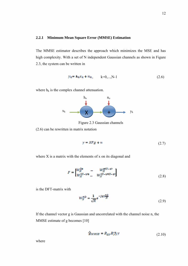
2.2.1 Minimum Mean Square Error (MMSE) Estimation
The MMSE estimator describes the approach which minimizes the MSE and has
high complexity. With a set of N independent Gaussian channels as shown in Figure
2.3, the system can be written in
, k=0,...,N-1 (2.6)
where hk is the complex channel attenuation.
yk
ho
Xxk
no
+
Figure 2.3 Gaussian channels
(2.6) can be rewritten in matrix notation
(2.7)
where X is a matrix with the elements of x on its diagonal and
(2.8)
is the DFT-matrix with
(2.9)
If the channel vector g is Gaussian and uncorrelated with the channel noise n, the
MMSE estimate of g becomes [10]
(2.10)
where

13
(2.11)
is the cross covariance matrix between g and y, Rgg is the auto-covariance matrix of g
and
(2.12)
is the auto-covariance matrix of y, σn2 denotes the noise variance E{|nk|2}.
Since the columns in F are orthonormal, frequency-domain MMSE, hMMSE can be
generated by gMMSE.
(2.13)
where
(2.14)
2.2.2 Least Square (LS) Estimation
Least Square (LS) method is about estimating parameters by minimizing the squared
discrepancies between observed data and their expected values. LS estimation
method attains low computational complexity, and it is easy to implement because it
does not require optimization procedures in its computation. The method is used to
solve imprecisely defined system [11]. The LS estimate of the attenuations h, given
the received data Y and the transmitted symbol X is [12].
(2.15)
This is reduced from
(2.16)

14
where
(2.17)
However, LS estimator has some limitations. It has high mean square error
which unable to give reasonable or correct estimates at all times. Since LS estimation
is a linear estimation scheme, it is not appropriate for the non Gaussian channel,
where in reality wireless channels do posses some non linear characteristics which
need to be considered for processing.
2.2.3 Kalman Filter Estimation
Kalman filter is the optimal estimate for linear system system models. In 1960, R.E
Kalman published his famous paper describing a recursive solution to the discrete-
data linear filtering problem. The Kalman filter is a set of mathematical equations
that provides an efficient computational (recursive) means to estimate the state of a
process, which minimizes the mean of the squared error [13]. It is very powerful in
several aspects: it supports estimations of past, present, and even future states, and
even when the nature of the modeled system is unknown.
The Kalman filter estimates a process by using a form of feedback control:
the filter estimates the process state at some time and then obtains feedback in the
form of noisy measurements. As such, the equations for the Kalman filter fall into
two groups: time update equations and measurement update equations. The time
update equations are responsible for projected forward the current state and error
covariance estimates to obtain the a priori estimates for the next time step. The
measurement update equations are responsible for the feedback for incorporating a
new measurement into the a priori estimate to obtain an improved a posterior
estimate.
The time update equation is also known as predictor equations, while the
measurement update equations can be thought of as corrector equations. The final
estimation algorithm resembles that of a predictor-corrector algorithm for solving
numerical problems as shown in Figure 2.3. It shows the ongoing discrete Kalman
filter cycle. The time update projects and the current state estimate ahead in time.
15
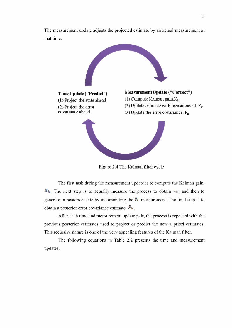
The measurement update adjusts the projected estimate by an actual measurement at
that time.
Figure 2.4 The Kalman filter cycle
The first task during the measurement update is to compute the Kalman gain,
. The next step is to actually measure the process to obtain , and then to
generate a posterior state by incorporating the measurement. The final step is to
obtain a posterior error covariance estimate, .
After each time and measurement update pair, the process is repeated with the
previous posterior estimates used to project or predict the new a priori estimates.
This recursive nature is one of the very appealing features of the Kalman filter.
The following equations in Table 2.2 presents the time and measurement
updates.

16
Table 2.2 Discrete Kalman filter time and measurement update equations.
Discrete Kalman filter time update equations
, (minus) shows the priori state estimate at step k.
= is the posterior state estimate at step k
Q = process noise covariance
, a priori estimate error covariance
where (a priori estimate errors) and
(a posterior estimate errors)
Discrete Kalman filter measurement update equations
= gain or blending factor that minimizes the a posterior error covariance,
R = measurement noise covariance
,
Where = measurement noise
is called the measurement innovation, or residual. The residual reflects the discrepancy between the predicted measurement, and the actual measurement . A residual of zero means that the two are in complete agreement.
, a posterior estimate error covariance
where

17
CHAPTER 3
AN OVERVIEW OF OFDM
3.1 Introduction
In this chapter, the basics of OFDM are discussed. In particular, a general description
and a brief history of OFDM are presented. In addition, the OFDM block diagram,
operation and signal processing are also explained briefly.
3.2 Overview of OFDM
OFDM technology was introduced back to the middle 60s. R.W. Chang [14] proved
that multiple data streams can be transmitted through a linear band limited multi-
channel without the ISI. The transmission of a band limited signal was synthesized
on multi-channel. For further improvement to suppress ISI, S.B. Weinstein [15]
made major contribution to OFDM in 1971 on how to modulate/demodulate band
signal by Discrete Fourier Transformation (DCT). Empty guard interval between two
adjacent symbols was proposed, but the orthogonality between two subcarriers over a
frequency selective channel cannot be ensured. To ensure the orthogonality among
subcarriers of an OFDM symbol, A. Peled [5] introduced the concept of cyclic prefix
(CP) in 1980. The CP is copied from the end of the OFDM symbol and was
transmitted followed by each OFDM symbol. Inter-carrier interference (ICI) can be
avoided when the length of CP is larger than the impulse response of the fading
channel.
OFDM is an efficient high data rate transmission technique for wireless
communication. It is a combination of multi-carrier modulation and multiplexing

18
techniques with high bandwidth efficiency and robustness in multipath and fading
environments where OFDM system is more resilient in Non Line-Of-Sight (NLOS)
environment. This is because of the equalization is done on a subset of sub-carriers
instead of a single broader carrier.
In OFDM, the communication system divides a wide radio channel into
several narrow sub-channels and data is transmitted in parallel on these sub-channels
on different frequencies or sub-carriers. Therefore, by creating the N parallel sub-
channels, the bandwidth of the modulation symbol are also by the factor of N. The
summation of all the individual sub-channels data rates will result in total desired
symbol rate, with the drastic reduction of the ISI distortion. The sub-carriers are
closely spaced to each other without causing interference, removing guard bands
between adjacent sub-carriers because the frequencies (sub-carriers) are orthogonal
(independent of each other). This means that the peak of one sub-carrier coincides
with the null of an adjacent sub-carrier as shown in Figure 3.1. The orthogonality
between sub-carriers prevents the demodulators from seeing frequencies other than
their own.
|S1(f)| |S2(f)| |S3(f)|
|SN(f)|
Sampling point
f3 f2 f1
Figure 3.1 The frequency division for OFDM systems

19
As seen, the spectra of the sub-carriers are not completely separated, but
overlap to some degree. With the so called orthogonality related method, it is the
reason why the information transmitted over the carriers can still be separated. From
the Figure 3.1 also, each sub-carrier is represented by a different peak. In addition,
the peak of each sub-carrier corresponds directly with the zero crossing of all
channels. To preserve perfect orthogonality, certain conditions need to be satisfied.
The receiver and the transmitter must be perfectly synchronized, which means they
both must assume exactly the same modulation frequency and the same time-scale
for transmission. A more important condition is that there should absolutely be no
multipath, which is solved by cyclically extending the symbol by a guard interval,
and the explanation of which is given in the following sections.
3.2.1 Basic Principles of OFDM System
A block diagram of a basic OFDM system is illustrated in Figure 3.2.
Figure 3.2 OFDM system
x s
T R A N S M I T T E R
R E C E I V E R
P/S
IFFT
S/P
QAM Mod.
Tx Bit Stream
(+) CP
Channel
Rx Bit Stream
P/S
FFT
QAM Demod.
S/P (-) CP
SNR Estimation

20
For high speed communications, principle of OFDM posits that frequency
selective channel is evenly divided into N frequency flat subchannels. At the
transmitter, random bits of data are coded and interleaved before modulation. The bit
stream is split into multiple parallel streams, which reduces the bit rate using serial-
to-parallel (S/P) converter. These bit streams lie in the frequency domain, so that
each element in vector bit streams is assigned to one subchannel. The generated
parallel data streams are modulated using QAM signal constellation to map them
individually on each subcarrier. IFFT is applied to these parallel bit streams to obtain
the time domain OFDM symbols. IFFT is used in OFDM system to infix the
orthogonal property between the subcarriers. The N subcarriers are transformed into
N point IFFT, with time domain representation of IFFT written as:
∑−
=
=1
0
2
).(1 N
k
Nnkj
ekXN
π
(3.1)
where X(k) is the symbol transmitted on the kth subcarrier and N is the total number
of subcarriers. Cyclic prefix (CP) is added to the transmitted symbol to avoid ISI
before the signal is transmitted.
At the receiver, the transmitted bit stream accumulates multipath fading
effects of channel. As the CP abides redundant information, removing it reduces the
complexity for FFT. The received signal is transformed into frequency domain using
N point FFT which can be given as
∑−
=
−
=1
0
2
).(1 N
k
Nnkj
enxN
π
(3.2)
X(k) on FFT is demodulated at N subcarrier frequencies relying on N demodulators
to convert them into parallel bit streams. The parallel bit streams are then converted
to serial bit stream using parallel-to-serial (P/S). The symbols are finally decoded to
obtain the transmitted information bits. A detailed system explanation of the function
for each block in Figure 3.2 is presented in the following sections.

21
3.2.2 Serial to Parallel Conversion
The data symbols are divided onto N parallel sub-carriers. This makes the symbols
on each sub-carrier N times longer than its serial counterpart. The effect of a time
dispersive channel is reduced by making the symbol duration longer than the
maximum excess delay of the channel. Each parallel data stream is modulated onto a
sub-carrier at a unique frequency and combined with the other sub-carriers to
produce a serial stream of transmission data. Proper selection of transmission
parameters can greatly reduce, if not eliminate ISI because the delay spread will be
less than the symbol duration.
3.2.3 Modulation
Binary data from a memory device or from a digital processing stream is used as the
modulating (baseband) signal. The following steps may be carried out in order to
apply modulation to the carriers in OFDM:
• Combine the binary data into symbols according to the number of bits/symbol
selected.
• Convert the serial symbol stream into parallel segments according to the
number of carriers, and form carrier symbol sequences.
• Apply differential coding to each carrier symbol sequence.
• Convert each symbol into a complex phase representation.
• Assign each carrier sequence to the appropriate IFFT bin, including the
complex conjugates.
3.2.4 IFFT Operation
S.B. Weinstein [3] proposed the idea of using the FFT to separate the sub-carriers in
the frequency domain. The complexity of OFDM implementation is greatly reduced
with the operation and can be easily incorporated into practical systems. As the
parallel sub-carriers of the signal transmitted are applied with IFFT, the spectrum is
transformed to the time domain to generate one symbol period.
22
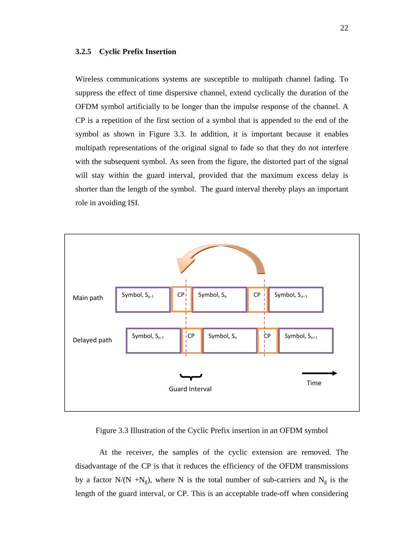
3.2.5 Cyclic Prefix Insertion
Wireless communications systems are susceptible to multipath channel fading. To
suppress the effect of time dispersive channel, extend cyclically the duration of the
OFDM symbol artificially to be longer than the impulse response of the channel. A
CP is a repetition of the first section of a symbol that is appended to the end of the
symbol as shown in Figure 3.3. In addition, it is important because it enables
multipath representations of the original signal to fade so that they do not interfere
with the subsequent symbol. As seen from the figure, the distorted part of the signal
will stay within the guard interval, provided that the maximum excess delay is
shorter than the length of the symbol. The guard interval thereby plays an important
role in avoiding ISI.
Symbol, Sn-1 Symbol, Sn Symbol, Sn+1 CP CP
Symbol, Sn-1 Symbol, Sn Symbol, Sn+1 CP CP
Main path
Guard IntervalTime
Delayed path
Figure 3.3 Illustration of the Cyclic Prefix insertion in an OFDM symbol
At the receiver, the samples of the cyclic extension are removed. The
disadvantage of the CP is that it reduces the efficiency of the OFDM transmissions
by a factor N/(N +Ng), where N is the total number of sub-carriers and Ng is the
length of the guard interval, or CP. This is an acceptable trade-off when considering
23
the advantages. A guard interval length of not more than 10% of the OFDM symbol
duration is employed.
3.2.6 Parallel to Serial Conversion
Once the CP has been inserted to the sub-carrier channels, they must be transmitted
as one signal. Thus, the parallel to serial conversion stage is the process of summing
all sub-carriers and combining them into one signal. As a result, all sub-carriers are
generated perfectly simultaneously.
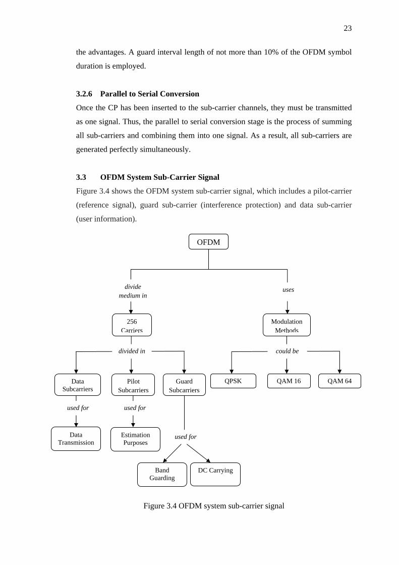
3.3 OFDM System Sub-Carrier Signal
Figure 3.4 shows the OFDM system sub-carrier signal, which includes a pilot-carrier
(reference signal), guard sub-carrier (interference protection) and data sub-carrier
(user information).
OFDM
divide medium in
uses
Data Transmission
Estimation Purposes
Band Guarding
DC Carrying
used for used for
used for
256 Carriers
Modulation Methods
Data Subcarriers
Pilot Subcarriers
Guard Subcarriers
divided in
QPSK QAM 16 QAM 64
could be
Figure 3.4 OFDM system sub-carrier signal

24
A sub-carrier is a modulation signal that is imposed on another carrier that
can be used to independently transfer information from other sub-carriers located on
the radio channel. The modulation techniques used can be QPSK, QAM 16 or QAM
64. The OFDM symbol structure is shown in Figure 3.5.
... ... ......
Pilot subcarriersDC subcarriers
Data subcarriers
Guard band subcarriers
Channel
Figure 3.5 OFDM symbol structure
The symbol consists of:
(a) Pilot sub-carriers as reference signal for use in the reception of other sub-
carrier signal and for various estimation purposes.
(b) Guard sub-carrier for keeping the space between OFDM signals dedicated for
communication channel protection from interference.
(c) Data sub-carriers carry information of data.
(d) DC sub-carrier as the referenced from the center of the radio channel.
The maximum number of carriers used by OFDM is limited by the IFFT size.
This is determined as in the following equation.
(real-valued time signal)
(complex-valued time signal)
In order to generate a real-valued time signal, OFDM (frequency) carriers are
defined in complex conjugate pairs, which are symmetric about the Nyquist
frequency (fmax). This results in the number of potential carriers to IFFT size / 2.
REFERENCES
1. Mobile WiMAX – Part I: A Technical Overview and Performance Evaluation,
2006 WiMAX Forum
2. Socheleau, F., Abdeldjalil Aἳssa-El-Bey and Houcke, S. Non Data-Aided SNR
Estimation of OFDM Signals , IEEE Communications Letters, Vol. 12, No.
11, November 2008
3. Pauluzzi D.R. and Norman C.B. A Comparison of SNR Estimation techniques
for the AWGN Channel, IEEE Transactions on Communications, Vol.48 no.
10, 2000
4. Boumard, S., Novel Noise Variance and SNR Estimation Algorithm for
Wireless MIMO OFDM Systems. IEEE GLOBECOME, VOL., 2003
5. A. Peled and A. Ruiz, Frequency domain data transmission using reduced
computational complexity algorithms, in Proc. IEEE ICASSP, vol. 5, pp. 964-
967, 1980.
6. Rana Shahid Manzoor, Wabo Majavu, Varun Joeti, Nidal Kamel and
Muhammad Asif, Front-End estimation of Noise Power and SNR in OFDM
Systems, IEEE-ICIAS vol., 2007, Pages 435-439
7. Reddy, S. And Arslan H. Noise Power and SNR Estimation for OFDM Based
Wireless Communication Systems. Wireless Communication and Signal
Processing Group, 2003
8. Xiadong X., Ya Jing and Xiaohu Y. Subspace-Based Noise Variance and
SNR Estimation for OFDM Systems. IEEE Wireless Communications and
Networking Conference, 2005
9. M. Wax and T. Kailath, Detection of signals by information theoretic criteria.
IEEE Transactions on Acoustics, Speech and Signal Processing, vol. 33, no.
2, pp. 387-392, 1985.
10. Louis L. Scharf, Statistical Signal Processing. Addison-Wesley, 1991.
11. Cleve B. Moler, Least Squares in Numerical computing with MATLAB, 1st
ed. Philadelphia, SIAM, 2004, ch.5, sec. 5.1-5.2, pp. 141, 143.
12. R. Van Nee and R. Prasad, OFDM for Wireless Multimedia Communications.
Artech House Publishers, Massachusetts, 2000.
13. M. Zivkovic and R. Mathar, Preamble-based SNR estimation in frequency
selective channels for wireless OFDM systems. IEEE 69th Vehicular
Technology Conf., Barcelona, 2009, pp.1-5.
14. R. W. Chang, Synthesis of band-limited orthogonal signals for multi-channel
data transmission. Bell System Technical Journal, vol. 46, pp. 1775-1796,
1966.
15. S. B. Weinstein and P. M. Ebert, Data transmission by frequency-division
multiplexing using the discrete Fourier transform. IEEE Trans.
Communication., vol. 19, no. 5, pp. 628-634, 1971.
16. IEEE 802.16a WMAN organization, Air Interface for Fixed Broadband
Wireless Access Systems. Part A : System between 2-11 GHz, April 2003.