social interaction an individual’s preferences, and therefore behaviour, may depend on what others...
TRANSCRIPT

Social Interaction
• An individual’s preferences, and therefore behaviour, may depend on what others in society are perceived to be doing.
• Learning (e.g. new technology and uncertainty).
• Social influence: a person’s preferences may be altered by those with whom the person interacts.
Social influence
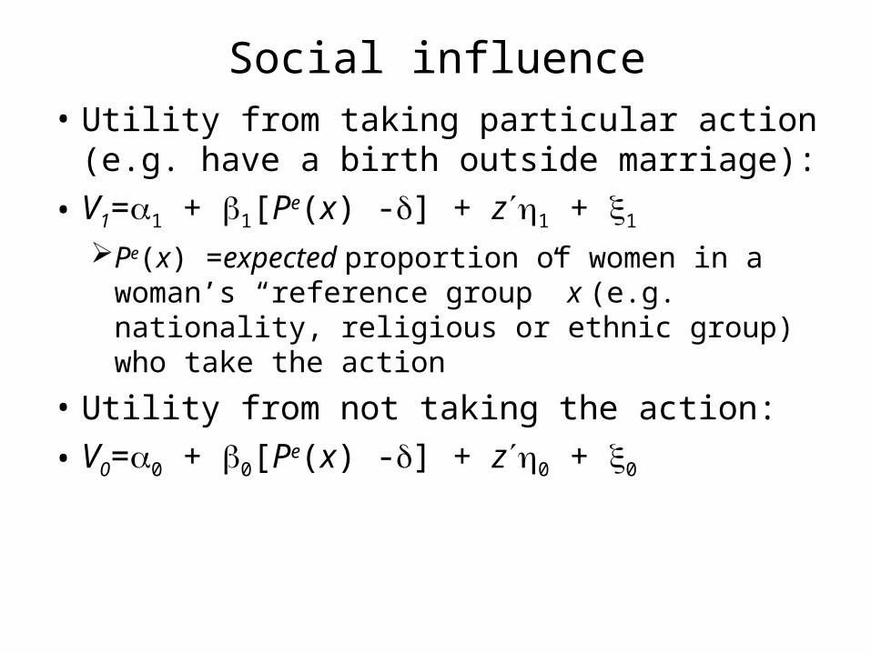
• Utility from taking particular action (e.g. have a birth outside marriage):
• V1=1 + 1[Pe(x) -] + z1 + 1
Pe(x) =expected proportion of women in a woman’s “reference group” x (e.g. nationality, religious or ethnic group) who take the action
• Utility from not taking the action:
• V0=0 + 0[Pe(x) -] + z0 + 0

Social influence/social stigma• Social, or “normative”, influences on utility are
indicated by the terms 1(Pe(x) -) and 0(Pe(x) -), with 00<1.
is a threshold parameter, such that when Pe(x)<, the expected proportion taking the action in a woman’s reference group exerts a negative influence on taking the action.a positive influence on not taking the action.
• the opposite is the case when Pe(x)>.• A value of Pe(x) below could reflect “social
stigma .

Other definitions• z=observable individual attributes (e.g.
educational attainment, wages, non-labour income) affecting utility in the two states.
1 and 0 are unobserved woman-specific variables affecting utility in the two states.
j may reflect policy variables (e.g. state benefits to single mothers (in which case 1> 0), cost and availability of abortion if action is non-marital birth).

Decision
• Take action if and only if V1>V0; that is, when =1-0>-{+[Pe(x) -] + z},
• where =1-0, =1-0 and =1-0.
• Social influence exists when >0
• ‘taste’ variable is assumed to have some random, symmetric (about the origin) distribution in the reference group population (e.g. logistic).

Probability of taking action
• the probability that a woman with reference group x takes the action is given by
• H[ + (Pe(x) -) + z]
• where H[] is a continuous, strictly increasing distribution function.

Proportion in reference group taking the action
The actual proportion in the reference group who take the action is
• P(x) = H[ + (Pe(x) -) + z]dP(z|x),
• where P(z|x) is the distribution of z in the reference group defined by x.

Social equilibrium
• A social equilibrium occurs when people’s expectations are consistent with the average proportion in the reference group who take the action.
• In equilibrium, people’s expectations are consistent with the mathematical expectation P(x).
• That is, Pe(x)=P(x).

Figure 11.1: Equilibrium Proportions becoming a Single Mother, "large" beta
Expected Proportion
Act
ual P
ropo
rtio
n

Figure 11.2: Equilibrium Proportions becoming a Single Mother, "moderate" beta
Expected Proportion
Act
ual P
rop
orti
on

Unique equilibrium or multiple equilibria?
• E.g. H[] is the logistic distribution function and +z is distributed symmetrically about the origin.
• If <4, there is a unique social equilibrium.
• If >4, then there are at least three social equilibria.

Why =4?
• In the neighbourhood of ‘middle’ equilibrium in Figure 1, at which P(x)=0.5, P(x)/Pe(x)>1.
• With the logistic distribution, P(x)/Pe(x)= P(x)[1-P(x)].
• Around middle equil, P(x)/Pe(x)=0.25.
• Implies P(x)/Pe(x)>1 in the neighbourhood of equil. requires >4.

>4 is not a sufficient condition for
multiple equilibria • E.g. the distribution of observable
attributes (z) is sufficiently skewed toward people who favour (are against) the action.
• Or the symmetry is not around the origin.
• Then there can be one high-level (low-level) equilibrium.

Figure 11.3: Equilibrium Proportions becoming a Single Mother, "large" beta
Expected Proportion
Act
ual P
ropo
rtio
n

Figure 11. 4: Equilibrium Proportions becoming a Single Mother, "large" beta
Expected Proportion
Act
ual P
ropo
rtio
n
Stability of equilibria and dynamics
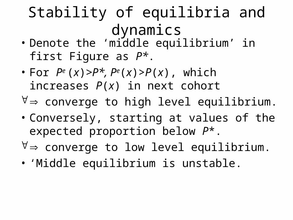
• Denote the ‘middle equilibrium’ in first Figure as P*.
• For Pe (x)>P*, Pe(x)>P(x), which increases P(x) in next cohort
converge to high level equilibrium.• Conversely, starting at values of the expected
proportion below P*. converge to low level equilibrium.• ‘Middle equilibrium is unstable.

Implications
• “History matters” (e.g. initial expectations) for the selection of the low-level or high-level equilibrium.
• Temporary changes in the socio-economic environment that alter behaviour and/or expectations can produce dramatic changes
move from low level to high level equilibirum

Multiplier effects (‘low’ , larger ) Figure 11.2: Equilibrium Proportions becoming a Single Mother,
"moderate" beta
Expected Proportion
Act
ual P
ropo
rtio
n

Shift in the distribution of attributes favourable to action from ‘skewed against’
Figure 11.3: Equilibrium Proportions becoming a Single Mother, "large" beta
Expected Proportion
Act
ual
Pro
por
tion

Shift from multiple equilibria to unique high level equilibrium, e.g. larger )
Figure 11. 4: Equilibrium Proportions becoming a Single Mother, "large" beta
Expected Proportion
Act
ual
Pro
por
tion

Example: rapid increase in non-marital childbearing in Europe
Figure 11.5: Percentage of Births Outside Marriage
0
10
20
30
40
50
60
IT GR
PO ESP IR AU
DE
-E
DE
-W GB
LU B
NL
FR FIN
SW DK
Country
1975 BoM
1997 BoM

Explosion of births outside marriage in BritainBirths Outside Marriage per 1000 Live Births
0
50
100
150
200
250
300
350
400
450
1845 1855 1865 1875 1885 1895 1905 1915 1925 1935 1945 1955 1965 1975 1985 1995Year

Who has a birth before marriage?
• Costs of non-marital birth in terms of labour and marriage market opportunities lost are smaller for women with ‘poorer prospects’ in these markets
• E.g. women with less education.
• Expect women with ‘poorer prospects’ to be more likely to have a birth before marriage.
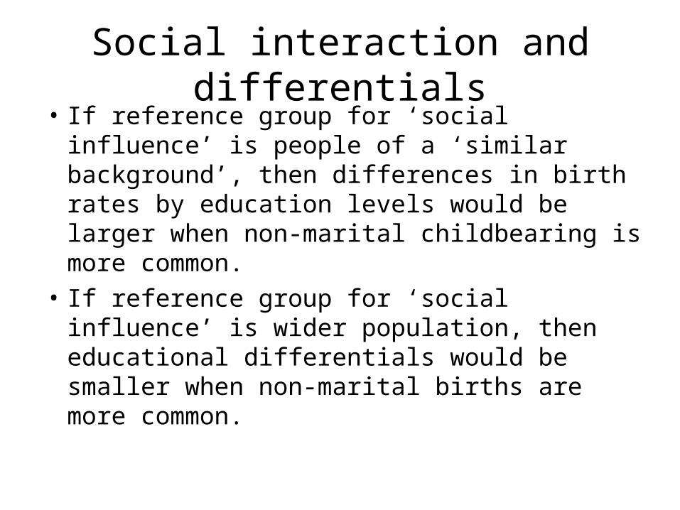
Social interaction and differentials• If reference group for ‘social influence’ is
people of a ‘similar background’, then differences in birth rates by education levels would be larger when non-marital childbearing is more common.
• If reference group for ‘social influence’ is wider population, then educational differentials would be smaller when non-marital births are more common.

Different equilibria by education group
Equilibrium Proportions becoming a Single Mother
Expected Proportion
Act
ual P
ropo
rtio
n
Comparison of birth rates
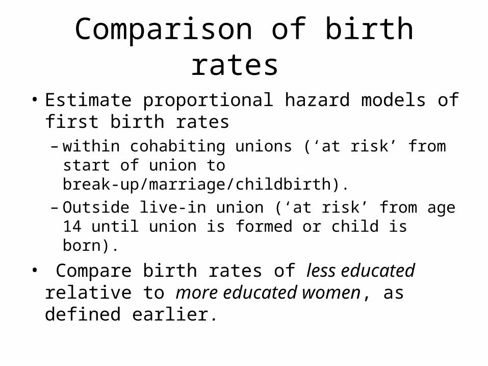
• Estimate proportional hazard models of first birth rates – within cohabiting unions (‘at risk’ from start of
union to break-up/marriage/childbirth).– Outside live-in union (‘at risk’ from age 14
until union is formed or child is born).
• Compare birth rates of less educated relative to more educated women, as defined earlier.

Birth rate: Low educ. relative to High educ. Women
0
0.5
1
1.5
2
2.5
3
3.5
4
4.5
5
Cohab union Outside union
1950s1960s1970s

Geographic clustering and social interaction
• If reference groups are within a country, country-clustering is consistent with a social interaction model with multiple equilibria (e.g. social stigma).
• Example: cohabiting unions in Europe.• Three broad groups in terms of the
percentage of women aged 25-29 who live in a cohabiting union.

Figure 11.6: Percentage of Births Outside Marriage (1997) and Pct. of Women aged 25-29 Cohabiting (1996) in 16 European Countries
R2 = 0.5977
0
10
20
30
40
50
60
0 5 10 15 20 25 30 35 40
Percent cohabiting
Pct
of
birt
hs o
utsi
de m
arri
age

Dramatic increase in cohabitation in Britain: Percent who cohabited in their first live-in
partnership, by birth cohort
0
10
20
30
40
50
60
70
80
90
1950s 1960s 1970s

Percent Cohabiting in First Union by Educational Attainment and Cohort
0
10
20
30
40
50
60
70
80
90
High Educ. Low Educ.
1950s1960s1970s

Cohabitation in first union
• Cohabitation was more likely for more educated women for women born in 1950s and 1960s.
• Less educated women had caught up by 1970s cohort.
• More educated were pioneers in cohabitation.

Markets and Multipliers
• Social multipliers and multiple equilibria can also arise through market interactions.
• E.g. positive social interaction mediated by the marriage market.
• Example 1: Divorce
• Example 2: The impact of the contraceptive pill on women’s career decisions

Divorce and prospects of remarriage• Divorce brings costs, because finding another
partner involves time and effort, and there is a risk of remaining single.
• The expected gain from divorce depends, therefore, on the prospects of remarriage.
• These prospects depend on the decisions of others to divorce and remarry.
a high-divorce or a low-divorce equilibrium may be supported with the same set of fundamental factors affecting divorce decisions.
Divorce and prospects of remarriage
• If many couples are expected to divorce, then the prospects of remarriage are high because there are more people in the remarriage market
divorce less costly more divorce.• Low divorce rates divorce more costly
fewer divorce.• the possibility of multiple equilibria (self-
fulfilling nature of divorce expectations).

Multiplier effects & search externalities
• Even if there is a unique equilibrium, an increase in the divorce rate generated by a small change in its fundamental determinants can give rise to a large change in the divorce rate.
• Because people do not take into account that one’s own divorce increases the remarriage chances of all other divorcees, the marriage market produces too few divorces inefficiency.
The Pill and Women’s Careers
• In the absence of reliable contraception, women undertaking lengthy professional education would have to incur – the cost of sexual abstinence – or the risk of pregnancy.
• The Pill decreased the cost of investment.
• Encouraged more women to enter professional careers.

The costs of delaying marriage
• Lengthy education generally requires the delay of marriage.
• In the interim other women marry.
• Career women are more likely to have to settle for a poorer match (smaller pool of eligible bachelors).
• Argument and evidence in C. Goldin and L. Katz (2000).
Indirect social multiplier effect• By reducing the penalty of delaying
marriage (sexual abstinence or pregnancy risk), the Pill encouraged all women and men to delay marriage to a time when their tastes and character were better formed.
• Created a better (“thicker”) marriage market for career women.
• Reduced the cost of delaying marriage.• Encouraged them to pursue a career.