soft-computing approaches for rescheduling problems in a
TRANSCRIPT

RAIRO-Oper. Res. 55 (2021) S2125–S2159 RAIRO Operations Researchhttps://doi.org/10.1051/ro/2020077 www.rairo-ro.org
SOFT-COMPUTING APPROACHES FOR RESCHEDULING PROBLEMSIN A MANUFACTURING INDUSTRY
Jaime Acevedo-Chedid1, Jennifer Grice-Reyes1, Holman Ospina-Mateus1,Katherinne Salas-Navarro2, Alcides Santander-Mercado3 and
Shib Sankar Sana4,∗
Abstract. Flexible manufacturing systems as technological and automated structures have a highcomplexity for scheduling. The decision-making process is made difficult with interruptions that mayoccur in the system and these problems increase the complexity to define an optimal schedule. Theresearch proposes a three-stage hybrid algorithm that allows the rescheduling of operations in an FMS.The novelty of the research is presented in two approaches: first is the integration of the techniquesof Petri nets, discrete simulation, and memetic algorithms and second is the rescheduling environmentwith machine failures to optimize the makespan and Total Weighted Tardiness. The effectiveness of theproposed Soft computing approaches was validated with the bottleneck of heuristics and the dispatchrules. The results of the proposed algorithm show significant findings with the contrasting techniques. Inthe first stage (scheduling), improvements are obtained between 50 and 70% on performance indicators.In the second stage (failure), four scenarios are developed that improve the variability, flexibility, androbustness of the schedules. In the final stage (rescheduling), the results show that 78% of the instanceshave variations of less than 10% for the initial schedule. Furthermore, 88% of the instances supportrescheduling with variations of less than 2% compared to the heuristics.
Mathematics Subject Classification. 90B35, 90B36, 68M20.
Received March 2, 2020. Accepted July 4, 2020.
1. Introduction
Competition forces organizations to act quickly to preserve their position in the market Flexible manufac-turing systems (FMS) allow the production of a variety of products to meet demand. FMS are the result oftechnological innovations generated through the years, where these problems are classified as highly complex(NP-Hard) [13]. The shop floor is a dynamic environment affected by the arrival of new activities, customer,and materials. The dynamic factors to consider are machine breakdowns, absenteeism from work, the arrival ofnew orders, and a change in the priority of work. Immediately consideration of dynamic factors in production is
Keywords. Flexible manufacturing system, scheduling, reactive scheduling, Petri net, memetics algorithm.
1 Department of Industrial Engineering, Universidad Tecnologica de Bolıvar, Cartagena, Colombia.2 Department of Productivity and Innovation, Universidad de la Costa, Barranquilla, Colombia.3 Department of Industrial Engineering, Universidad del Norte, Barranquilla, Colombia.4 Kishore Bharati Bhagini Nivedita College, Behala, Kolkata 700060, India.∗Corresponding author: [email protected], shib [email protected]
Article published by EDP Sciences c© EDP Sciences, ROADEF, SMAI 2021

S2126 J. ACEVEDO-CHEDID ET AL.
known as reactive or real-time schedules [34]. Seeking the optimization of manufacturing processes, inventoriesand manufacturing costs has a significant impact on the organizational management of a company, and thesehave impacts on the decision-making process [10,15,16,23,32,48]. The plant floor will always require optimizedtasks, to better meet all customers’ requirements [40,41,47]. The processes are aimed to be sustainable, efficient,and profitable [36,50,56]. Customers will recognize the effective management of an organization by factors suchas quality, time, opportunity, and economy in goods and services [24,51,59].
The research proposes a three-stage hybrid algorithm that allows the rescheduling of operations in an FMS.The novelty of the research is presented in two approaches: One is integration of the techniques of Petri nets,discrete simulation, and memetic algorithms and second is rescheduling environment with machine failuresto optimize the makespan and Total Weighted Tardiness. The hybrid algorithm was called “PetNMA”. ThePetNMA algorithm is composed of three (3) sub algorithms. The first performs the initial scheduling of thejobs. The second simulates the initial scheduling until the machine fails, so a rescheduling is required. Thethird generates a reactive scheduling through the application of a memetic algorithm. The proposed algorithmis validated with problems of the FMS library. The results of the initial scheduling are compared with thebottleneck and dispatch rules, and the reactive scheduling was compared with the dispatch rules.
The model has a novel proposal that integrates the Petri net technique as an effective method for productionscheduling. The innovative component of the proposed model has two key elements. First integrates the Petrinets with a genetic algorithm to develop active initial scheduling and second integrates the use of memeticalgorithms with Petri nets for a production rescheduling environment. The integration of Petri net starts fromthe generation of active schedules and their configuration when the machine failure occurs. This research isconsidered a pioneer in a memetic algorithm decoded by Petri nets in an environment of rescheduling whenthere are failures or breakdowns of machines.
The proposed model establishes a modification of the libraries with different ranges of scenarios. The failureof the machine is considered in four instances with the fault simulations in different periods. This analysisidentifies the flexibility and robustness of production schedules. This paper is organized as follows: the theoreticalframework and literature review are in Section 2. In Section 3, the applied methods are described, such as Petrinets, genetic algorithms, memetic algorithms, simulated annealing, and local search. In Section 4, the algorithm“PetNMA” is presented and explained. In Section 5, the results obtained with the “PetNMA” algorithm. Thefindings, conclusions, and discussion are in Section 6.
2. Background and literature review
Production scheduling is the assignment and sequence of jobs to resources for the manufacture of goods orservices [45]. Production schedule are aimed at optimizing deadlines, delivery times, setups, inventories, and theuse of machines [45]. There are many methods and strategies used to develop a production schedule [5]. Amongthe basic and efficient strategies are the well-known dispatch rules. These consider the allocation and sequencingbased on delivery dates, processing time, machine loading, among other strategies, as follows: Shortest ProcessingTime (SPT), Largest Processing Time (LPT), Most Remaining Work Time (MRWT), Earliest Due Date (EDD),Critical Ratio (CR), Apparent Tardiness Cost (ATC), and Minimum Slack (MSLACK). The objectives are usedto evaluate the most important production schedule are: Makespan, Maximum Tardiness, Total Tardiness, TotalWeighted Tardiness, Total Flow, and Total Weighted Flow [45].
2.1. Flexible manufacturing system (FMS)
An FMS is a system with a technological and automated component that can produce a variety of operationsand tasks for production. The route of a job within the system is flexible and is taken in the scheduling process.An FMS be a flexible job shop with an additional number of restrictions [44]. The flexibility within a productionsystem allows us to diversify products, anticipate demand, forecast inventory, increase the efficiency and qualityof processes [28,49,53].

SOFT-COMPUTING APPROACHES FOR RESCHEDULING PROBLEMS IN A MANUFACTURING INDUSTRY S2127
Low and Wu [31] symbolically represented the FMS as a set of machines MT = {m1,m2, . . . ,mM} anda set of jobs J = {J1, J2, . . . , JN}, where each job Jj ,∀j ∈ {1, 2, . . . , N} has a delivery date dj promisedand it consists of a sequence of nj operations. Each operation Oi,j ,∀i ∈ {1, 2, . . . , N} and ∀j ∈ {1, 2, . . . , ni},it can be processed continuously on any machine mk of set of machines MS , (MS ⊆MT ) in a processing timepi,j,k, it is including setup time on the machine. Each machine mk, ∀k ∈ {1, 2, . . . ,M} can process only oneoperation. It is assumed that all pi,j,k, dj and nj are deterministic as well as the jobs available (rj = 0,∀j).From an Operations Research perspective, scheduling in FMS is a more complex version of the classic flexiblescheduling problem, which is known to be NP-hard [13]. This complexity is caused by the versatility, flexibility,and alternate routes in the operations. An FMS contains many variables and restrictions that change over time,and these characteristics justify the use of dynamic scheduling [28].
2.2. Reactive scheduling
Random events involve the rescheduling of production, which affects initial scheduling and the level of cus-tomer service. This action is known as reactive scheduling [11]. The dynamic production environment is exposedto constant adjustments. Among them: machine failures, the arrival of new jobs, change of priorities, job cancel-lation, supplier failures, low-quality materials, absenteeism, and variability in jobs (processing times or deliverydates), changes in due dates. Most of the approaches to reactive scheduling or rescheduling, had been based onthe generation of a basic predictive schedule. The three most common methods for rescheduling are: regeneration,partial rescheduling, and right-shift scheduling [60]. Regeneration includes all operations. Partial reschedulingonly considers affected operations. The right shift method postpones the remaining operations; This methodleads to more stable schedules.
2.3. Machine failure or breakdowns
One of the most frequent random events is machine failure or breakdown. This event may require twotypes of rescheduling. Total repair or reprocessing of the schedule. Repair refers to the local configuration ofthe current schedule, while the total rescheduling of a new schedule is generated from the base. To addressrescheduling, machine failures must determine which jobs have been completed and which are affected. A job iscalled “complete” if it is completed before the failure. A task is considered “affected” if it needs to be relocateddue to the interruption. Reactive scheduling is based on the affected jobs [19].
In a manufacturing system, the unavailability of a machine can be known in advance and better managed,compared to when an unexpected failure occurs. A robust schedule is one that can contain interrupts, such asevents that were considered in their original planning [2]. The probability of failure of the machines is quantifiedby the time the machine has been occupied divided by the total time. A machine with higher occupancy is morelikely to fail. If a manufacturing system has historical data to provide an approximate distribution of machinefailures, it can be used to predict the time of machine failure and repair time to obtain a robust and stablepredictive schedule [33].
2.4. Literature review
The literary review synthesizes the previous contributions of authors in the field of flexible manufacturingsystems and their scope in reactive scheduling or rescheduling. In summary, Table 1 outlines all these findings.
Hatono et al. [20] used a Stochastic Petri Nets to describe the uncertain events of stochastic behavior inthe FMS, such as machine failures, repair time, and processing time. Cho [8] developed a Petri net model formessage manipulation and event monitoring in an FMS cell. ElMaraghy and Elmekkawy [12] proposed schedulingalgorithm that used Petri nets to deal with machine faults in real-time. Chen and Chen [6] simulated a Petrinet in its method for non-hierarchical control for the performance of an FMS. Chen and Chen [7] developed analgorithm for the rescheduling of random events such as machine failures in an FMS. Acevedo and Mejıa [1]carried out a Genetic Algorithm for reactive scheduling in FMS with arrivals of new jobs and priority changes.

S2128 J. ACEVEDO-CHEDID ET AL.
Table 1. Contributions of previous authors.
Author(s) Production
system
Scheduling
strategy
Rescheduling
strategy
Event Objective(s) Petri nets Heuristic(s)
Hatono et al. [20] FMS Petri nets Hierarchical
structures
Machine failures,
repair and, pro-
cessing time
Total time Stochastics FMS simula-
tion
Cho [8] Shop Floor
Control Sys-
tem (SFCS)
Petri nets × × Equipment,
workstation,
and shop
Interpreted
petri nets
Hierarchically
decomposed
ElMaraghy and
ElMekkawy [12]
FMS Petri nets Deadlock-free Machine break-
downs
Total time Timed and
minimal
siphons
×
Chen and Chen
[6]
FMS Petri nets Client-server
paradigm
Object-oriented
approach
Total time Colored
Petri net
simulation
×
Chen and Chen
[7]
FMS Adaptive
scheduling
Rolling horizon Machine failures,
repair time
Completion
time
× Markov pro-
cess
Kumar et al. [27] FMS Fuzzy-based Operation
machine allo-
cation vector
Machine loading
problem
System
imbalance,
throughput
Extended
neuro-fuzzy
Petri net
×
Acevedo and
Mejıa [1]
FMS Petri nets Reactive schedule Machine break-
downs, new jobs
Total time Timed Petri
nets
Memetic
algorithm
Mejia and
Acevedo [34]
FMS Reactive
scheduling
Simulation Machine break-
downs, new jobs
Total time Timed Petri
nets
Genetic algo-
rithm
Tanimizu et al.
[54]
FMS Reactive
scheduling
Based reactive Delay and new
jobs
Total time × Genetic algo-
rithms
Kim et al. [25] FMS Reactive
scheduling
RTA* and rule-
based supervisor
Due date Total time,
tardiness
Timed Petri
net
A reactive
fast graph
Tashnizi et al.
[55]
FMS × × Sharing resources
and processing
times
Total time Petri net ×
Tuysuz and
Kahraman [58]
FMS Petri nets
fuzzy sets
× Uncertainty in
system
Time-critical Stochastic Fuzzy
mathematics
Zhao et al. [61] FMS Petri nets × Discrete events Total time Timed Petri
net
Genetic
algorithm
Patel and Joshi
[43]
FMS Petri nets,
simulation
deadlock
× × Throughput,
completion
time
Stochastic ×
Han et al. [17] FMS Petri nets,
deadlock
× × Makespan Timed petri
net
Genetic
algorithm
Baruwa et al. [4] FMS Petri nets,
deadlock-free
× × Makespan Timed
colored
Petri net
Anytime
heuristic
search algo-
rithm
Basak and
Albayrak [3]
FMS Petri nets,
real-time
scheduling
× × Timed
marked
graph
Object-
oriented
Petri nets
Artifex PN
Han et al. [18] FMS Petri nets,
deadlock
× Lot sizes,
resource capaci-
ties, and routing
flexibility
Makespan Timed Petri
net
Simulated
annealing,
swarm
optimization
Li et al. [30] FMS Petri nets × Available time of
shared resources
Makespan Transition-
timed Petri
nets
Heuristic
search
function
Lei et al. [29] FMS Petri nets,
deadlock
× Deadlock-free Makespan Timed Petri
nets
Heuristic
search
strategies
Mejıa and Nino
[35]
FMS Petri nets × × Makespan Timed place
petri net
Beam search
strategy
Huang et al. [22] FMS Petri nets × × Makespan Timed place
petri net
Ordered
binary
decision
diagrams
This paper FMS Petri nets
Active
schedule
Reactive, Robust,
Simulation
Machine break-
downs
Makespan,
tardiness
Timed Petri
nets
Genetic
algorithm,
simulated
annealing,
local search

SOFT-COMPUTING APPROACHES FOR RESCHEDULING PROBLEMS IN A MANUFACTURING INDUSTRY S2129
Mejia and Acevedo [34] development an integrated system of Petri nets to model an FMS. They presented aprototype that simulated the production plan and implemented dispatch rules to resolve possible conflicts.
Tanimizu et al. [54] developed a genetic algorithms of continuous rescheduling for the arrival of new jobs. Kimet al. [25] presented a new method for an FMS based on Petri nets and a reactive graphical search algorithm,looking for the minimization of the makespan and the total tardiness. Tashnizi et al. [55] develop a Petri netswith non-linear scheduling. Tuysuz and Kahraman [58] modeled a flexible manufacturing cell using stochasticPetri nets with fuzzy parameters. Patel and Joshi [43] developed a model for an FMS with deadlock and analyzedit to generate the reachability tree using Petri net system. Han et al. [17] proposed a scheduling method thatprovides a new approach to evaluate the performance of different deadlock controllers with Petri nets and geneticalgorithms. Baruwa et al. [4] investigated a deadlock-free scheduling method for an FMS based on timed coloredPetri nets with a heuristic.
Basak and Albayrak [3] presented a Petri net-based decision system modeling in real-time scheduling andcontrol of an FMS. Han et al. [18] proposed an effective hybrid particle swarm optimization algorithm with atimed Petri net model to solve the deadlock-free scheduling problem of an FMS. Li et al. [30] modeled schedulingproblems with a transition timed Petri net and an improved heuristic function that also considers the availabletime of shared resources within an FMS. Lei et al. [29] solved a deadlock-free scheduling of FMS with thecontrolled backtracking strategy based on the execution of the Petri nets. Mejıa and Nino [35] developed a fastand efficient Beam Search strategy based on Petri Nets for FMS scheduling. Huang et al. [22] developed an FMSscheduling based on binary decision diagram and Petri net.
Based on the state-of-the-art review, several studies have addressed the problem of scheduling and reschedul-ing due to machine failure in an FMS. Research has focused on developing efficient algorithms, improvingperformance metrics, time and computational cost. In recent years, the use of genetic algorithms combined withlocal search techniques has been emphasized to obtain better results. However, the results found by its authorsare still susceptible to improvement, through the development of new hybridization structures. In this subject,new applications are always required to improve the computational process in its structure, compilation, andintegration. These innovations always allow us to find better solutions.
This study presents a new hybrid algorithm construction that combines the Petri Nets and Genetic Algorithmfor the initial schedule. This combination allows the achievement of very good solutions within active schedulesin environments of an FMS. In reactive rescheduling due to machine breakdowns, the Petri Nets and MemeticAlgorithms are integrated with local search techniques and Simulated Annealing. The integration allows robustschedules after the occurrence of machine failure and unavailability. The proposed model allows us to avoid con-flicts, blocks, and implement real-time controls. The proposed model is justified by its robustness and stability,the ability to manage uncertainty due to machine failure, its resilience and flexibility to adapt easily to differentcircumstances. Finally, the novelty of the research is to consider the integration of efficient scheduling methods.Additionally, it is proposed to optimize two important metrics (makespan and tardiness) and simulate failuresby scenarios to analyze in context of the complexity of an FMS.
3. Method and material
In this section, we describe Petri Nets, Genetic Algorithms, Memetic Algorithms, Simulated Annealing, andLocal Search, as backgrounds.
3.1. Petri Net
A Petri Net (PetN) is a directed graph, heavy and bipartite, consisting of places, transitions, and arcs, wherethe arcs go from a place to a transition or a transition to a place. In the graphical representation places arerepresented by circles, transitions for bars, and bows by arrows. A marking on the PetN indicates the distributionof an integer (positive or zero) token for each position [8]. Murata [38] formally defined Petri Nets as six-folderpresentation PetN = (P, T,O, I,M,W ), where:
• n, number of places in the PetN.

S2130 J. ACEVEDO-CHEDID ET AL.
• m, number of transactions in the PetN.• P = {p1, p2, . . . , pn} is set of n places are drawn as circles, for n > 0.• T = {t1, t2, . . . , tm} is set of m transitions are drawn as bars or boxes, with P ∪ T 6= 0 and P ∩ T = 0 form > 0.
• O : T × P → N is the set of input arcs directed from T to P , where N = {0, 1, 2, . . .}.• I : P × T → N is the set of output arcs directed from P to T , where N = {0, 1, 2, . . .}.• M(p) : P → N is the marking in the pth place or the token number in the pth place at some point. An initial
labeling is denoted by M(0). Tokens (black dots) reside in places and represent the truth of the conditionof action associated with the corresponding place. Tokens move throughout the net by effect of transitionfirings.
• W is the set of weights associated with the arcs.
For purposes of simplifying the other definitions in the Petri Nets, Murata [38] use the following symbolicrepresentations, which have been adopted for purposes of this research:
• K(p), the maximum number of tokens that can hold the place p.• w(p, t), weight of the arc that communicates the place p with the transition t.• w(t, p), weight of the arc that communicates the transition t with the place p.• •t, set of places of input to the transition t.• t•, set of output locations transition t.• •p, set of input transitions to place p.• p•, set of output transitions to place p.• R(M(0)), set of possible markings made from M(0).• L(M(0)), the set of sequences to fire M(0).• C = {Ci,j}, incidence matrix of n×m, such that if all weights are assumed as one, so: Ci,j = 1 if the placei is an output place for the transition j, Ci,j = −1 if the place i is an input place for the transition j, andCi,j = 0 otherwise.
In Petri nets, a transition t is said to be enabled if all its input places are marked at least w(p, t) tokens.Also, a transition can be fired if enabled. When a transition is fired, w(p, t) tokens are removed from their inputplaces and they put w(t, p) tokens in their output places, considering the constraints of the system. A transitionwithout input place is called an enabled transition, while a transition without output place is a final transition.A transition t and a place p form a loop if p is, at the same time, input, and output place of t.
One of the great advantages of the application of Petri nets to real systems is the ability to monitor theirevolution. The evolution of the net allows us to identify the movements of the tokens between the places, whichin turn define the vector of marking and its changes in time. If in a finite capacity PetN transition t fires, itis satisfied that the number of tokens in each output place p of that transition, does not exceed its maximumcapacity K(p), which is represented by: M ′(p) +w(t, p) ≤ K(p). The equations of state make use of C = {Ci,j},where Ci,j = C+
i,j − C−i,j , with C+
i,j = w(i, j) and C−i,j = w(j, i). The evolution of the system from one step toanother, is represented by the equation of state M(k + l) = M(k) + C · u(k), where M(k) represents vectormarking, after of k fired transitions, l the net change in the tokens in place i when transition j is fired, andu(k) the vector transition firing, which contains zeros except jth position containing a 1, indicating that jthtransition is fired after k events. If a marking M(d) destination is reachable from M(0) through a firing sequence{u1, u2, . . . , ud}, the state equation is written as: M(d) = M(0) + C ·
∑dk=1 u(k), or as ∆M = C ·X, if makes
M(d) −M(0) = ∆M and∑d
k=1 u(k) = X, with X column vector whose input the jth position is the numberof times the transition has been fired j. Figure 1 illustrates a Petri Nets model of an FMS with two jobs.
The benefit of using the Petri Nets as a tool for modeling the systems is the knowledge about the state ateach moment of its evolution using the vectors of markings. It is known as the evolution of the network everystep it takes over time, that is, the movement of the tokens between the places after the fire of the transitions.Two types of properties of the Petri Nets have been identified, those that depend on the initial state or marking

SOFT-COMPUTING APPROACHES FOR RESCHEDULING PROBLEMS IN A MANUFACTURING INDUSTRY S2131
Figure 1. Petri Nets model for FMS with two jobs and three machines [1].
of the Petri Nets, called behavioral, and the properties that depend on the structure of the network, calledstructural. The marking of a Petri Net changes after each fire a transition.
Petri Nets have been widely used for the scheduling and rescheduling of production in manufacturing systems.A Petri Nets is most often used as a tool to model and control the production process in an FMS [3,18, 22, 29,35, 39]. Due to the graphic nature, descriptive capacity, Petri Net as a powerful tool to play an important rolein modeling and analysis [27,28,43].
3.2. Memetic algorithm
Memetic Algorithm (MA) is an optimization technique that combines other metaheuristics (population-basedsearch and local improvement). The MA is based on individual improvements of the solutions in each of theagents along with cooperation processes and competitions. Moscato and Cotta [37] related the origins of MAin the late eighties when evolutionary strategies and genetic algorithms began to take advantage. The nameMemetic comes from the term meme introduced by Richard Dawkings to represent a unit of cultural evolution.In the context of optimization, a meme represents a learning or development strategy. MA contributes to thesolution of production scheduling in optimal or near-optimal solutions, avoiding local minima or prematureconvergence [9]. MA convergence is treated with local search techniques [14].
The MA starts from a genetic algorithm, it plays an important role in its structure. They constitute theglobal search tool providing the coverage of diversity while the local search provides the intensification. Geneticalgorithms are part of the evolutionary algorithms that constitute a general technique for solving search andoptimization problems [46]. The form in which evolutionary algorithms work is related to how species evolvein nature. Genetic algorithms use a set of possible solutions or individuals to calculate adaptation measures.Through an iterative process this population changes and each iteration are called generation. For an individualto survive and pass on to the next generation it must have a high level of adaptation and participate in geneticoperations, with which new individuals are created who constitute the next generation. These algorithms allow usto address problems of great complexity of search and optimization. The most popular evolutionary algorithmsare given its efficiency and ease of implementation. Solutions are represented as a bit string before being decoded.The behavior is defined as the following parameters: the size of the initial population, the number of generations,the percentages of mutation and crossover. A schematic representation of the procedure of the genetic algorithmis shown in Figure 2.
Next, the simulated annealing, and the local search are related, as a hybrid strategy within the memeticalgorithms. Local search is a search process in the space of possible solutions. The search begins for a random

S2132 J. ACEVEDO-CHEDID ET AL.
Pseudo-code
P1.Generate Initial population
P1.1. Define a genetic representation of the system (Chromosome
Representation).
P1.2 Generate a random population of n chromosomes (Initial Population).
P2. Evaluate the level of adaptation of each chromosome in the population
(Evaluate the fitness).
P3. Create a new population (Next Generation)
P3.1. Select two chromosomes parents of a population according to their level
of adaptation (Selection mechanism).
P3.2. Chromosomes reproduce among themselves according to a predefined
crossover probability, create a new offspring (the children) (Crossover)
P3.3. Genes of a resulting child individual are exchanged according to the
mutation probability(Mutation).
P3.4 The best % individuals generate the of the children at the next
generation(Elitism )
P3.5. Place the new offspring in a new population (New Generation).
P4. The algorithm terminates after a predefined number of generations or if
after several generations, the algorithm has not found a better solution
(Termination Criterion).
Figure 2. Flow diagram and pseudocode of a genetic algorithm.
solution and then focuses on neighboring solutions iteratively. Iterations are made by setting a parameter bythe memory of the found solutions [21]. The local search has as components: a search space, a set of feasiblesolutions, a neighborhood relation, an initialization function, a step function, and a completion condition.Simulated annealing was proposed by Kirkpatrick et al. [26] motivated by the annealing of the solids, a processin which the solids are heated and subsequently cooled slowly to obtain perfect crystal structures. The main ideaof SA is an observed analogy between a complex system optimization and a description of the physical behaviorof a system. This method is applied in many domains: operational research, production scheduling, and manyothers. Simulated annealing can be considered as a process in which in a neighborhood you try to move fromone current solution to another of your neighbors. SA generates a new solution S′ in the neighborhood of thecurrent solution, then calculates the change d = C(S′) − C(s), where C(s) the value of the objective functionof the initial solution. The algorithm must be designed using certain methods to represent solutions, generateneighboring solutions, and reduce the temperature. The parameter T decreases gradually by a cooling functionuntil a stop condition is satisfied.
4. Problem definition, assumptions, and notation
This section contains problem definition, assumptions followed by notation are used such as it is much easierto understand the model. The hybrid PetNMA algorithm is composed of three (3) sub algorithms. The firstperforms the initial scheduling of the jobs. The second simulates the initial scheduling until the machine failsthat results a rescheduling. The third generates a reactive scheduling through the application of a memeticalgorithm.
4.1. Notation
The notation used to represent mathematically what happens with the set of operations that enter the reactivescheduling of the production is the following:
n : number of places.
The places are operational (O) or resources (R): P = {p1, p2, . . . , pn} = O ∪R.
m : number of transitions.ump : vector of enabled transitions.Xi,j,k : time when the ith operation of the job j on the machine k starts in the initial schedule.

SOFT-COMPUTING APPROACHES FOR RESCHEDULING PROBLEMS IN A MANUFACTURING INDUSTRY S2133
pi,j,k : processing time of the ith operation of the jth job on the machine k.Ci,j,k : completion time of the ith operation of the jth job on the machine k.Oi,j,s : ith operation of jth job on a machine of workstation s.OR
i,j,k : ith operation of jth job on kth machine.TR
k : time availability of kth machine reactive scheduling.α : percentage of the makespan in the weighted objective.β : percentage of total weighted tardiness in the weighted objective.CONP : set of undeveloped operations.PSize : represents the GA parameter, associated with the size of the population.nbd : represents the number of faults of simulated machines.r : rth reactive scheduling activity, due to failure number r = (1, 2, . . . , nbd).tbd : instant when the failure occurs.NTPI : number of transitions programmed to be fired in the initial schedule.NES(tbd) : number of transitions fired during the simulation until the moment of failure.ng : number of genes that make up the chromosome.ngr : number of genes that make up the chromosome for reactive scheduling, due to failure r.ngr−1 : number of genes that formed the chromosome in reactive scheduling, due to the failure r − 1. When
r = 1, ng0 = 2∑N0
j=1 nj .
The operational place represents the action “Operation Oi,j,k in process” and the conditions “job avail-able”, “job completed” and “job Waiting at workstation s”. The resource places represent the “availability of amachine”, where the initial marking of the resource places is 1 for all resources. All resource places are untimed.
4.2. Assumptions
The problem of reactive scheduling due to machine failures in an FMS, is formally declared with the followingassumptions:
(1) The FMS is composed of a set of machines MT = {m1,m2, . . . ,mk, . . . ,mM} and a set of work ordersJ = {J1, J2, . . . , Jj . . . , JN}.
(2) Each work order Jj has a delivery date dj committed to the customer, a priority defined by their level ofimportance wj and consists of a sequence of operations Oj = {O1,j , O2,j , . . . , Oi,j , . . . , Onj ,j}∀j.
(3) Each machine mk∀k can process only one operation until failure P (Fault)k occurs in the scheduling horizon.(4) Assumed that all pi,j,k, dj and wj are deterministic and processing time pi,j,k includes the time of prepa-
ration or setup on the machine. Where k represents the index of machines (k = 1, 2, . . . ,M), j is the indexof work orders (j = 1, 2, . . . , N), and i is the index of operations (i = 1, 2, . . . , nj).
(5) Each workstation s has a space at the beginning which is used for temporary storage of all jobs will beprocessed. where s is the index of workstations (s = 1, 2, . . . , S).
(6) When a job is completely processed in a workstation, it is moved to the next workstation or inventory offinished products.
(7) The interruption of the scheduling is generated due to machine failures.(8) In the reactive scheduling, the operations are in process in a machine without failure, i.e., are not inter-
rupted. Any operation that is being processed on a machine that fails, will be break and will have to bereinitialized.
(9) All operations conform to reschedule operations that have not been done and the operations are affectedby the failure of the machine.
(10) The objective functions considered here is to minimize Makespan (Cmax = max(Cj)), Total WeightedTardiness (
∑Nj=1 wjTj) and weighted objective (αCmax + β
∑Nj=1 wjTj) with α+ β = 1.

S2134 J. ACEVEDO-CHEDID ET AL.
Figure 3. PetNMA: Reactive scheduling algorithm of an FMS with machine failure.
4.3. Scheduling and system simulation
The PetNMA algorithm is based on a series of sub-algorithms which develop in a sequence of three stages:Sub-algorithm of Scheduling, Sub-algorithm of Simulation and Sub-algorithm of Reactive Scheduling (see Fig. 3).
4.3.1. Sub-algorithm scheduling
The sub-algorithm is to structure an initial production schedule in an FMS with all jobs j, using modelingPetri nets, the algorithm for obtaining active schedules, and genetic algorithms. The sub-algorithm is supportedby the LEKIN software. The initial scheduling is constructed, by establishing the sequence of fired transitionssupported by the dispatch rules (SPT, LPT, MRWT, EDD, CR, ATC, and MSNACK). The Sub-algorithmScheduling has the objective of obtaining active schedules. Therefore, genetic algorithms are applied to obtainnew schedules. In the implementation of the Sub-algorithm Scheduling in Microsoft Visual Studio 2010, theformat of the Petri net class was taken from the Afs-Petrinet Algorithm [1] and adapted to represent machinefailures. Below are the detailed steps of the Sub-algorithm Scheduling (see Algorithm 1).

SOFT-COMPUTING APPROACHES FOR RESCHEDULING PROBLEMS IN A MANUFACTURING INDUSTRY S2135
Algorithm 1. Initial scheduling.
The genetic algorithms notice that the completion of an operation requires the firing of a pair of transitions:The first transition of the pair marks the start and the second represents the termination of any operation. Thedecoding is based on the work done by Mejia and Acevedo [34], e.g., take Figure 4 and the following chromosome:The three transitions that are enabled at this state conform the array ump(0) = [t1, t2, t5]. Transitions are putinto the array in lexicographic order. The remainder of the integer division between the first gene (6) and thesize (3) of the array ump is 0. Thus transition t1 in the 0th position of ump is selected to fire. Transition t1is fire and changes the state of the net, generating a new vector of enabled transitions ump(1) = [t3, t5] (seeFig. 4). The second gene (77) is taken. The remainder of the gene (77) and the size of the array (2) is 1 andthe 1th position is selected. This corresponds to transition t5. The process is repeated until reaching the finalmarking.
4.3.2. Sub-algorithm simulation
To perform a simulation of the events we must consider the vector of fired transitions obtained in theScheduling Sub algorithm. This vector relates the times in which each operation must be performed. This list of

S2136 J. ACEVEDO-CHEDID ET AL.
Figure 4. Example of chromosome decoding.
events to be performed varies with time as each event takes place. However, the operations are carried out in somemachines can present failures. This is what should be done reactive scheduling or rescheduling of production.Previously, it is necessary to perform a simulation of the execution of operations that have been programmedand machine failures. It should be noted that it does not have historical data, which is why the failure to generatethe methodology used by Mehta [33]. To determine the time when the failure occurs the normal probabilitydistribution is used, to determine the machine fault, since all machines have the same probability of failure.However, in this study to determine the repair time of the machine we use the Log-Normal distribution toestablish the failure time (Repair time). The time of each failure or repair time, is given by LN(ln(γ1p), γ2).Where, ln(γ1p) is the average of the function, p is the average processing time of the system, γ1 is the percentageof p which is part of the repair timeand γ2 is the variance. Below are the detailed steps of the Sub-algorithmSimulation of scheduled events and failures of machines (see Algorithm 2).
Algorithm 2. Sub-algorithm simulation – Part A.
To carry out the Reactive scheduling in PetNMA, all the operations that at the time of the failure hadnot been executed must be considered, as well as the operation that was being processed in the machine atthat moment, forming the set CONP. The operations that were being processed during the failure inoperablemachines are not interrupted until they have been completed. The following is a series of steps to obtain thelist of those operations (see Algorithm 3).
Algorithm 3. Sub-algorithm simulation – Part B.

SOFT-COMPUTING APPROACHES FOR RESCHEDULING PROBLEMS IN A MANUFACTURING INDUSTRY S2137
Table 2. Route of the operations of two jobs in a manufacturing system with four machines.
Operation Job 1 Job 2
(Operation 1) M1(6) M2 (7)(Operation 2) M3 (8) o M4 (8) M4 (5)
4.3.3. Sub-algorithm of reactive scheduling
When a machine failure occurs during the development of the Sub-algorithm, the rescheduling must be donethrough the Sub-algorithm Reactive Scheduling. For this scheduling, all operations in CONP must be considered.The MA used consists of an evolutionary algorithm and a local search technique. The GA was selected for theevolutionary part. Meanwhile, as a local search technique, the simulated annealing algorithm runs after eachgeneration. The Sub-algorithm Reactive Scheduling is composed of the following steps (see Algorithm 4).
Algorithm 4. Sub-algorithm of reactive scheduling.
5. Experimental evaluation
The experimental tests were developed by running on a Dell Inspiron computer with an Intel Inside CORE I5processor, 8 gigs of RAM, 1 TB of memory, and Windows 7. The algorithms were developed in Microsoft VisualStudio 2010 in C++ language.
5.1. Numerical illustration of the sub-algorithm scheduling
To better understand this stage of the algorithm, corresponding to phase 1 of the Sub-algorithm Scheduling,an example of its application is specified using a numerical example. A manufacturing system develops two (2)jobs with two (2) operations with an established sequence and four (4) machines in the system. The path ofeach job is shown in Table 2, where the process times of each operation are shown in parentheses.
The modeling system described above is as follows:The input and output functions of Petri nets used to represent the manufacturing system in Figure 5, can
be represented using the following incidence matrices (Tabs. 3–5):In the present study, the Timed Petri Nets were used to model the FMS together with the random faults of
the machines. In Figure 6, the system represented above can be evidenced with additional places and transitions

S2138 J. ACEVEDO-CHEDID ET AL.
Figure 5. PetN model for a Job Shop with two jobs, four machines.
Table 3. Positive incidence matrix for the job shop represented in Figure 5.
p0 p1 p2 p3 p4 p5 p6 p7 p8 p9 p10 p11 p12 p13 p14
t0 0 1 0 0 0 0 0 0 0 0 0 0 0 0 0t1 0 0 1 0 0 0 0 0 0 0 0 1 0 0 0t2 0 0 0 1 0 0 0 0 0 0 0 0 0 0 0t3 0 0 0 0 0 1 0 0 0 0 0 0 0 1 0t4 0 0 0 0 1 0 0 0 0 0 0 0 0 0 0
C+ = t5 0 0 0 0 0 1 0 0 0 0 0 0 0 0 1t6 0 0 0 0 0 0 0 1 0 0 0 0 0 0 0t7 0 0 0 0 0 0 0 0 1 0 0 0 1 0 0t8 0 0 0 0 0 0 0 0 0 1 0 0 0 0 0t9 0 0 0 0 0 0 0 0 0 0 1 0 0 0 1
Table 4. Negative incidence matrix for the job shop represented in Figure 5.
p0 p1 p2 p3 p4 p5 p6 p7 p8 p9 p10 p11 p12 p13 p14
t0 −1 0 0 0 0 0 0 0 0 0 0 −1 0 0 0t1 0 −1 0 0 0 0 0 0 0 0 0 0 0 0 0t2 0 0 −1 0 0 0 0 0 0 0 0 0 0 −1 0t3 0 0 0 −1 0 0 0 0 0 0 0 0 0 0 0t4 0 0 −1 0 0 0 0 0 0 0 0 0 0 0 −1
C− = t5 0 0 0 0 −1 0 0 0 0 0 0 0 0 0 0t6 0 0 0 0 0 0 −1 0 0 0 0 0 −1 0 0t7 0 0 0 0 0 0 0 −1 0 0 0 0 0 0 0t8 0 0 0 0 0 0 0 0 −1 0 0 0 0 0 −1t9 0 0 0 0 0 0 0 0 0 −1 0 0 0 0 0

SOFT-COMPUTING APPROACHES FOR RESCHEDULING PROBLEMS IN A MANUFACTURING INDUSTRY S2139
Table 5. Incidence matrix for the job shop represented in Figure 5.
p0 p1 p2 p3 p4 p5 p6 p7 p8 p9 p10 p11 p12 p13 p14
t0 −1 1 0 0 0 0 0 0 0 0 0 −1 0 0 0t1 0 −1 1 0 0 0 0 0 0 0 0 1 0 0 0t2 0 0 −1 1 0 0 0 0 0 0 0 0 0 −1 0t3 0 0 0 −1 0 1 0 0 0 0 0 0 0 1 0t4 0 0 −1 0 1 0 0 0 0 0 0 0 0 0 −1
C = t5 0 0 0 0 −1 1 0 0 0 0 0 0 0 0 1t6 0 0 0 0 0 0 −1 1 0 0 0 0 −1 0 0t7 0 0 0 0 0 0 0 −1 1 0 0 0 1 0 0t8 0 0 0 0 0 0 0 0 −1 1 0 0 0 0 −1t9 0 0 0 0 0 0 0 0 0 −1 1 0 0 0 1
Figure 6. Petri Net model for a Job Shop with 2 jobs, 4 machines, considering machine failures.
that correspond to the machines under repair after a failure. Transitions machine failures are fired when thecorresponding machine simulation has failed while the operation is processed. For this, one must consider theMk vector marking at the time the machine fails. When the corresponding transition is fired, the token thatis in the operation place is removed and two tokens are added to the place corresponding to the repair of themachine and to the available job place (if the operation was the initial one) or to the queue from a job. Atthe end of the repair time of the machine, the corresponding transition is fired, and the token is returned to themachine so that it is available again.
Where, Op. 1 Operation 1; Op. 2 Operation 2; Op. 2.1 Operation 2 option 1; Op. 2.2 Operation 2 option 2;M1 Machine 1; M2 Machine 2; M3 Machine 3; M4 Machine 4; RM1 Repair of the machine 1; RM2 Repair ofthe machine 2; RM3 Repair of the machine 3; RM4 Repair of the machine 4; T0, T3, T6, T12 Transitions thatstart operations; T1, T4, T7, T10, T13 Transitions that end operations; T2 Failure M1 while working in Op. 1of job 1; T5 M3 failure while working in Op. 2.1 of job 1; T8 M4 failure while working in Op. 2.2 of job 1; T11M2 failure while working in Op. 1 of job 2; T14 M4 failure while working in Op. 2 of job 2; T15 Enables M1after being repaired; T16 Enables M2 after being repaired; T17 Enables M3 after being repaired; T18 EnablesM4 after being repaired. When the failure of a machine is generated, the rescheduling of the activities must becarried out with many strategies, through the sub-algorithm of reactive scheduling.

S2140 J. ACEVEDO-CHEDID ET AL.
Table 6. Description of the 10 problems chosen to perform the experimental tests.
No. of problem No. of jobs No. of workstations No. of machines
1 6 10 192 9 8 203 10 5 104 10 5 125 10 5 126 10 7 187 10 10 208 15 5 129 15 6 1710 20 6 13
5.2. Experimental tests of the scheduling sub algorithm in PetNMA
To obtain the initial schedules with the Scheduling Sub algorithm in PetNMA, ten (10) problems thatcharacterize an FMS were used (see Appendix A). Problems that were used for testing were adapted from theproblems developed by Mejia and Acevedo [34] and the classic problems LA and ORB. Each problem has a fewjobs to be scheduled in a few workstations and machines (see Tab. 6).
– The route of the work by stations in the FMS consists of times each of their operations. These times wereset randomly within the range [36,37], to obtain variability problems.
– In the classical problems, the assignment of the machines to each of the workstations is performed randomlywithin the interval [10,13,34]. An assignment of machines stations than three (3) system produces downtimemachines throughout the scheduling.
– The job weights were assigned randomly considering the uniform distribution within the interval [10,13,34].– In the delivery times of each work, the total work rule (TWK) was used, where dj = kPj , where Pj is the
sum of the process times of all operations of work j and k. However, a normal distribution with a range[1.3, 1.5] was used to give more diversification to the delivery times.
– In designing experiments to validate the parameters, the problems according to the number of jobs in small,medium, and large are classified. Considering the classification problems from 1 to 3 correspond to small,from 4 to 7 to medium and from 8 to 10 to large.
To evaluate the performance of the Scheduling Sub algorithm in PetNMA, the results have been comparedwith the dispatch rules SPT, LPT, MRWT, CR, ATC, MSLACK, and with the results obtained with thebottleneck. The comparison is made between the objective functions evaluated, in this case the makespan,total weighted tardiness, and weighted objective. For each of the objectives it has conducted a factorial designexperiment to choose the best parameters for the genetic algorithm. The parameters chosen for the bullfightswere taken from previous studies identified in the literature review. Three types of problems (small problem (2),medium problem (7), and large problem (9)) are chosen to perform the parametrization runs in the experimentaldesign (see Tab. 7). The results of the runs, the experiment design and its graphs are in Appendix B. In thecase of the weighted objective, the tests were carried out with all the weighting options for alpha and beta withone decimal, to choose the combination that finds the best results, varying them simultaneously from 0 to 1. Inaccordance with the tests and the experimental design and Pareto graphs, the weighted objective combinationwas selected 50–50. Considering the results obtained, the following values were chosen for the parameters of thegenetic algorithm of the Initial Scheduling Sub algorithm:
Next, the results of 10 runs of each of the 10 problems studied are shown with the parameters chosen foreach problem (see Tabs. 8–10).

SOFT-COMPUTING APPROACHES FOR RESCHEDULING PROBLEMS IN A MANUFACTURING INDUSTRY S2141
Table 7. Parameters selected for the genetic algorithm of initial Scheduling in PetNMA.
Makespan TWT Weighted objective
Parameters Nomenclature Values S M B S M B S M B
Number of
generations
Maxgen 100; 200 100 100 100 200 200 200 200 200 200
Size of the
initial
population
P 100 100 100 100 100 100 100 100 100 100
Probability of
crossing
Tc 60%; 90% 60% 60% 60% 90% 90% 90% 60% 60% 90%
Probability of
mutation
Tm 10%; 50% 50% 50% 50% 50% 50% 50% 50% 50% 50%
Intensity of
mutations
Im 1; 2; 4 2 2 2 4 4 4 4 4 4
Elitism Te1 Off, On 25%; 50% 50% 50% Off 50% 50% 50% 50% 50% 50%
Notes. S: Small; M: Medium; B: Big.
Table 8. Results of the initial sub-algorithm scheduling in PetNMA for minimization Makespan.
Problem Bottleneck Dispatch rules
SPT LPT MRWT EDD CR ATC M. SLACK Min
FMS01 412 436 464 436 464 436 436 464 436
FMS02 316 377 346 346 377 324 324 361 324
FMS03 536 726 757 536 703 632 632 593 536
FMS04 395 470 483 401 487 483 489 418 401
FMS05 412 476 472 390 516 447 447 506 390
FMS06 342 332 382 357 375 352 352 349 332
FMS07 1143 1152 1146 1149 1110 1132 1155 1209 1110
FMS08 470 561 559 459 574 569 552 555 459
FMS09 269 288 288 263 298 261 275 299 261
FMS10 753 836 935 759 814 912 873 779 759
Problem Active schedules with dispatch rules Genetic algorithm
SPT LPT MRWT EDD CR ATC M. Min Min Max Average
SLACK
FMS01 480 456 412 480 456 456 456 412 436 436 436
FMS02 369 357 326 377 341 367 361 326 324 324 324
FMS03 736 754 536 856 632 662 771 536 536 536 536
FMS04 483 478 395 524 465 569 478 395 394 394 394
FMS05 541 475 379 555 515 469 512 379 390 390 390
FMS06 408 468 368 394 380 398 379 368 332 332 332
FMS07 1291 1198 1164 1149 1158 1160 1323 1149 994 1036 1019.3
FMS08 682 581 487 671 582 633 693 487 442 459 453.8
FMS09 394 344 287 396 318 328 291 287 249 256 252.7
FMS10 924 977 800 995 845 999 809 800 753 753 753

S2142 J. ACEVEDO-CHEDID ET AL.
Table 9. Results of the initial sub-algorithm scheduling in PetNMA for minimization TWT.
Problem Bottleneck Dispatch rules
SPT LPT MRWT EDD CR ATC M. SLACK Min
FMS01 0 0 0 0 0 0 0 0 0
FMS02 0 0 0 0 0 0 0 0 0
FMS03 1716 1919 2525 2387 2332 2177 2130 2183 1919
FMS04 50 208 390 205 326 152 404 183 152
FMS05 156 226 669 472 347 410 519 240 226
FMS06 0 0 130 0 0 0 0 0 0
FMS07 359 1852 1946 0 2672 1325 1917 2415 2369 1325
FMS08 304 548 1882 1043 648 477 995 439 439
FMS09 0 4 310 421 1 69 205 1 1
FMS10 5891 8449 11 815 12 099 7347 10 642 11 293 8647 7347
Problem Active schedules with dispatch rules Genetic algorithm
SPT LPT MRWT EDD CR ATC M. Min Min Max Average
SLACK
FMS01 0 10 0 0 0 0 0 0 0 0 0
FMS02 0 0 0 0 3 29 0 0 0 0 0
FMS03 2008 2656 2418 3676 2158 2462 2733 2008 1577 1604 1581.6
FMS04 202 454 349 295 159 706 131 131 40 40 40
FMS05 446 1172 1014 829 679 702 614 446 144 169 155.5
FMS06 210 436 0 27 37 85 0 0 0 0 0
FMS07 3761 3079 3375 1793 2300 2664 4041 1793 476 630 563.5
FMS08 1896 2518 1933 1634 755 2065 936 755 150 294 230.2
FMS09 902 1126 654 396 186 731 0 0 0 0 0
FMS10 11 041 14 153 13 321 9160 11 586 15 680 9309 9160 6159 6944 6564.5
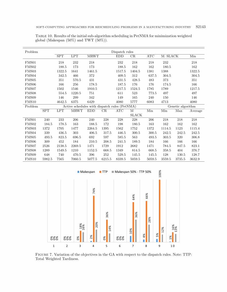
According to the results in the first phase of the algorithm, significant results were obtained using the GA (seeFig. 7). Makespan was improved in 50% of the instances. In these instances, an average improvement of 4% wasachieved. Total weighted tardiness improved in 70% of instances. In these instances, an average improvementof 53% was achieved. The weighted objective (Makespan 50% – TWT 50%) achieved an improvement in 70%of the instances. The average improvement in these instances was 20%. The initial scheduling sub-algorithm inPetNMA has improved the results in the larger instances by comparing them with the dispatch and bottleneckrules, because in small instances the same results can be achieved in the first cycles of the sub-algorithm.
5.3. Experimental tests of the reactive scheduling sub algorithm in PetNMA
To obtain the reactive schedules with the Reactive Sub-algorithm Scheduling in PetNMA, a design of exper-iments was carried out using the three selected problems. For each of the objectives was conducted TaguchiRobust Design to choose the best parameters for the GA considering factors that cannot be controlled whenhaving a breakdown machine. The factors considered to assess the performance of algorithm: Control factors(A: Number of generations, B: Size of the population, C: Probability of crossing, D: Probability of mutation,E: Intensity of mutations, F: Elitism, G: Factor decremental) and Noise factors (H: Instance of the fault,I: Variation of repair time, J: Mean time to repair). Failure scenarios two forms were generated, depending onwhen the scheduling horizon in which the failure occurs, the percentage of the average processing time used forthe repair time of the machine, and the time variation repair. The scenarios can be identified using the followingcoding: B(Cx, γ1, γ2) where, Cx corresponds to the medium and takes values from 1 to 2, γ1 corresponds tothe percentage of the average processing time and takes values 0.5 and 1.0, and γ2 represents the variation
SOFT-COMPUTING APPROACHES FOR RESCHEDULING PROBLEMS IN A MANUFACTURING INDUSTRY S2143
Table 10. Results of the initial sub-algorithm scheduling in PetNMA for minimization weightedglobal (Makespan (50%) and TWT (50%)).
Problem Dispatch rules
SPT LPT MRWT EDD CR ATC M. SLACK Min
FMS01 218 232 218 232 218 218 232 218
FMS02 188.5 173 173 188.5 162 162 180.5 162
FMS03 1322.5 1641 1461.5 1517.5 1404.5 1381 1388 1322.5
FMS04 342.5 466 372 409.5 312 637.5 304.5 304.5
FMS05 351 570.5 431 431.5 428.5 483 373 351
FMS06 166 256 178.5 187.5 176 176 174.5 166
FMS07 1502 1546 1910.5 1217.5 1524.5 1785 1789 1217.5
FMS08 554.5 1220.5 751 611 523 773.5 497 497
FMS09 146 299 342 149 165 240 150 146
FMS10 4642.5 6375 6429 4080 5777 6083 4713 4080
Problem Active schedules with dispatch rules (PetNMA) Genetic algorithm
SPT LPT MRWT EDD CR ATC M Min Min Max Average
SLACK
FMS01 240 233 206 240 228 228 228 206 218 218 218
FMS02 184.5 178.5 163 188.5 172 198 180.5 163 162 162 162
FMS03 1372 1705 1477 2264.5 1395 1562 1752 1372 1114.5 1123 1115.4
FMS04 339 436.5 303 406.5 317.5 446.5 300.5 300.5 242.5 242.5 242.5
FMS05 493.5 823.5 696.5 692 597 585.5 563 493.5 303.5 320 306.8
FMS06 309 452 184 210.5 208.5 241.5 189.5 184 166 166 166
FMS07 2526 2138.5 2269.5 1471 1729 1912 2682 1471 784.5 847.5 823.1
FMS08 1289 1549.5 1210 1152.5 668.5 1349 814.5 668.5 358.5 404 376.7
FMS09 648 740 470.5 396 252 529.5 145.5 145.5 128 130.5 128.7
FMS10 5982.5 7565 7060.5 5077.5 6215.5 8339.5 5059.5 5059.5 3559.5 3735.5 3632.9
Figure 7. Variation of the objectives in the GA with respect to the dispatch rules. Note: TTP:Total Weighted Tardiness.

S2144 J. ACEVEDO-CHEDID ET AL.
Table 11. Values for MA in sub-algorithm of reactive scheduling.
Makespan TWT Weighted objectiveParameters S M B S M B S M B
Number of generations 100 100 100 200 200 200 200 100 200Size of the initial population 100 100 50 100 100 50 50 100 50Probability of crossing 90 90 60 60 60 90 90 90 90Probability of mutation 10 50 10 50 50 50 10 50 50Intensity of mutations 1 2 1 2 2 2 4 4 1Elitism 50 0 0 0 0 50 0 0 50Factor decremental 0.1 0.01 0.01 0.1 0.1 0.01 0.1 0.01 0.01
Notes. S: Small; M: Medium; B: Big.
Figure 8. Percentage of improvement of the final objective with respect to the rules of dispatch.
with values of 0.02 and 0.05. According to the results obtained in the experimental design (see Appendix B)the following values have been selected for the memetic algorithm of the Reactive Scheduling Sub algorithm inPetNMA (Tab. 11).
The small problem always gets the best result both for the makespan and for the Total weighted tardiness inthe first generation because few operations must be programmed in a few machines, so the dispatch rules getgood schedules. For the total weighted tardiness, both the small problem and the large one gets good answers,the medium problem has high delays because most of the jobs start in the same stations and therefore, theyare bottled in them. For the weighted objective, good results are obtained in the small and large instances, thesame inconvenience of the total weighted tardiness in the medium instances is had. The results and graphs ofthe designs of the experiments carried out can be seen in Appendix C. Next, the results of a run of each of the10 problems studied are shown in the Tables 12–14.
Considering the results, we can present the following conclusions of the experimental tests developed:
– 95%, 85%, and 85 of the results in the rescheduling of production with PETNMA generated improvementsbetween 0% and 2% with respect to the values obtained by the dispatch rules for the makespan. Totalweighted tardiness and the objective weighted respectively. 12% of the instances evaluated have improvementsgreater than 2% (see Fig. 8).
– The algorithm was able to generate different variations in the different instances and rescheduling minimizedthose variations. On average 58% of the results had variations between 0% and 2% with respect to the initialscheduling. 33% of the instances had variations between 2% and 60%. While 10% exceeded 100% variations(see Fig. 9).
For the weighted objective, in scenarios 1 and 4, the machine failure occurs in the first half of the ini-tial scheduling horizon shows that the variation of the final scheduling is greater than the initial scheduling.

SOFT-COMPUTING APPROACHES FOR RESCHEDULING PROBLEMS IN A MANUFACTURING INDUSTRY S2145
Table 12. Results of the PetNMA for the evaluation of the Makespan.
Instance Failure Schedule SPT LPT MRWT EDD CR ATC M. SLACK Memetic Variation (%)
scenario initial algorithm
FMS01 6 10 19
1 412 468 468 468 1566 1497 1578 1000 452 9.71
2 412 413 413 413 826 751 810 630 413 0.24
3 412 412 412 412 537 492 513 487 412 0.00
4 412 412 412 412 1162 1074 1141 695 412 0.00
FMS02 9 8 20
1 324 324 324 324 2215 2009 2217 591 324 0.00
2 324 324 324 324 647 578 636 489 324 0.00
3 324 324 324 324 533 505 529 400 324 0.00
4 324 324 375 324 1467 1296 1454 636 324 0.00
FMS03 10 5 10
1 536 632 624 536 1711 1388 1726 949 536 0.00
2 536 623 623 623 623 623 623 623 623 16.23
3 536 536 536 536 573 573 573 537 536 0.00
4 536 719 711 623 1581 1264 1522 1001 623 16.23
FMS04 10 5 121 394 406 426 394 1655 1471 1675 1136 394 0.00
2 394 394 394 394 918 763 918 762 394 0.00
3 394 394 394 394 873 763 868 736 394 0.00
4 394 417 432 401 2224 1934 2247 1162 394 0.00
FMS05 10 5 12
1 379 437 472 406 1665 1314 1672 856 406 7.12
2 379 408 408 408 417 408 408 417 408 7.65
3 379 420 420 420 420 431 431 431 420 10.82
4 379 491 472 438 2222 2048 2198 807 438 15.57
FMS06 10 7 18
1 332 332 349 332 1536 1279 1541 581 332 0.00
2 332 404 439 367 1226 1040 1238 573 359 8.13
3 332 332 335 332 1133 858 1117 566 332 0.00
4 332 332 351 333 2314 2030 2278 632 332 0.00
FMS07 10 10 20
1 1012 1032 1091 1061 3878 3704 3884 2780 1032 1.98
2 1012 1015 1051 1015 1998 1806 1969 1573 1015 0.30
3 1002 1002 1002 1002 1808 1592 1811 1401 1002 0.00
4 1002 1007 1089 1007 3746 3502 3686 2660 1007 0.50
FMS08 15 5 12
1 451 464 489 1477 1806 1471 1772 1073 464 2.88
2 451 544 544 544 544 544 544 544 544 20.62
3 456 583 526 493 1479 1351 1523 1012 493 8.11
4 448 580 586 514 2842 2441 2871 1335 499 11.38
FMS09 15 6 17
1 253 264 269 259 1736 1513 1754 861 259 2.37
2 254 274 274 274 288 299 299 299 274 7.87
3 254 271 271 271 286 299 299 299 271 6.69
4 254 273 276 259 1578 1282 1578 930 259 1.97
FMS10 20 6 13
1 753 758 767 753 1634 1422 1605 1478 753 0.00
2 753 804 839 782 1274 1130 1274 1293 782 3.85
3 753 813 813 813 813 813 813 813 813 7.97
4 753 758 935 754 2722 2387 2698 2291 754 0.13
Average variation 4.21
Figure 9. Percentage of variation of the final objective with respect to the initial scheduling.
S2146 J. ACEVEDO-CHEDID ET AL.
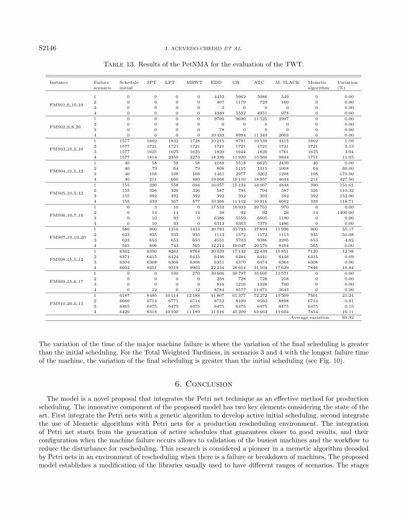
Table 13. Results of the PetNMA for the evaluation of the TWT.
Instance Failure Schedule SPT LPT MRWT EDD CR ATC M. SLACK Memetic Variation
scenario initial algorithm (%)
FMS01 6 10 19
1 0 0 0 0 4452 5962 5086 549 0 0.00
2 0 0 0 0 407 1179 720 160 0 0.00
3 0 0 0 0 2 0 0 0 0 0.00
4 0 0 0 0 4349 5532 4951 978 0 0.00
FMS02 9 8 20
1 0 0 0 0 9700 9690 11 525 2997 0 0.00
2 0 0 0 0 0 0 0 0 0 0.00
3 0 0 0 0 78 0 0 0 0 0.00
4 0 0 0 0 10 433 8994 11 349 2003 0 0.00
FMS03 10 5 10
1 1577 1602 1832 1728 10 215 9791 10 539 4415 1602 1.59
2 1577 1721 1721 1721 1721 1721 1721 1721 1721 9.13
3 1577 1625 1625 1625 1820 1644 1820 1761 1625 3.04
4 1577 1814 2350 2273 18 336 11 920 15 360 9844 1751 11.03
FMS04 10 5 12
1 40 58 58 58 4188 5518 6625 2439 40 0.00
2 40 79 64 79 808 1115 1311 1008 64 60.00
3 40 108 108 108 1461 2977 3262 1208 108 170.00
4 40 211 660 480 19 068 19 116 18 957 4644 211 427.50
FMS05 10 5 12
1 155 390 558 694 16 057 15 124 14 067 4848 390 151.61
2 155 326 326 326 587 794 794 587 326 110.32
3 155 392 392 392 392 392 392 392 392 152.90
4 155 339 567 577 10 366 11 112 10 916 6662 339 118.71
FMS06 10 7 18
1 0 3 10 0 17 552 18 933 20 755 970 0 0.00
2 0 14 14 14 38 92 92 26 14 1400.00
3 0 10 93 0 6386 5559 6605 1190 0 0.00
4 0 10 93 0 6313 6363 7370 1486 0 0.00
FMS07 10 10 20
1 580 900 1216 1433 30 793 35 793 37 894 11 996 900 55.17
2 623 935 935 935 1113 1572 1572 1113 935 50.08
3 623 653 653 653 4551 5703 9386 2295 653 4.82
4 565 806 743 565 12 214 19 047 20 570 8494 565 0.00
FMS08 15 5 12
1 6302 8390 8263 8764 20 039 17 132 22 439 15 851 7120 12.98
2 6371 6415 6424 6415 6446 6484 6441 6446 6415 0.69
3 6304 6308 6308 6308 6351 6370 6474 6364 6308 0.06
4 6602 9351 9319 9903 22 234 26 654 31 504 17 629 7846 18.84
FMS09 15 6 17
1 0 0 100 270 39 606 30 797 35 605 11 571 0 0.00
2 0 0 0 0 258 728 728 258 0 0.00
3 0 0 0 0 816 1216 1328 700 0 0.00
4 0 12 0 12 8784 8577 11 671 3643 0 0.00
FMS10 20 6 13
1 6187 8486 10 114 12 188 41 807 61 377 72 272 15 509 7501 21.24
2 6660 6714 6771 6714 8752 8109 9562 8898 6714 0.81
3 6465 6475 6475 6475 6475 6475 6475 6475 6475 0.15
4 6420 8318 10 100 11 189 31 016 45 209 63 663 19 604 7454 16.11
Average variation 69.92
The variation of the time of the major machine failure is where the variation of the final scheduling is greaterthan the initial scheduling. For the Total Weighted Tardiness, in scenarios 3 and 4 with the longest failure timeof the machine, the variation of the final scheduling is greater than the initial scheduling (see Fig. 10).
6. Conclusion
The model is a novel proposal that integrates the Petri net technique as an effective method for productionscheduling. The innovative component of the proposed model has two key elements considering the state of theart. First integrate the Petri nets with a genetic algorithm to develop active initial scheduling, second integratethe use of Memetic algorithms with Petri nets for a production rescheduling environment. The integrationof Petri net starts from the generation of active schedules that guarantees closer to good results, and theirconfiguration when the machine failure occurs allows to validation of the busiest machines and the workflow toreduce the disturbance for rescheduling. This research is considered a pioneer in a memetic algorithm decodedby Petri nets in an environment of rescheduling when there is a failure or breakdown of machines. The proposedmodel establishes a modification of the libraries usually used to have different ranges of scenarios. The stages

SOFT-COMPUTING APPROACHES FOR RESCHEDULING PROBLEMS IN A MANUFACTURING INDUSTRY S2147
Table 14. Results of the PetNMA for the evaluation of the weighted objective.
Instance Failure Schedule SPT LPT MRWT EDD CR ATC M. SLACK Memetic Variation
scenario initial algorithm (%)
FMS01 6 10 19
1 206 222 232 222 2519 3459 3126 1376.5 213 3.40
2 206 206 206 206 296 368 370.5 253.5 206 0.00
3 206 209 209 209 227 246.5 246.5 223 209 1.46
4 206 220 224 224 1814.5 1628 1733.5 844.5 220 6.80
FMS02 9 8 20
1 162 162 162 162 6355.5 5001.5 7551.5 790 162 0.00
2 162 162 162 162 1580 1461 2017.5 229.5 162 0.00
3 162 162 162 162 452 729 907.5 240 162 0.00
4 162 168.5 167 167 9826.5 7813.5 9952.5 478.5 167 3.09
FMS03 10 5 10
1 1114.5 1559.5 1686.5 1569 5821.5 4393 4736.5 2535.5 1490.5 33.74
2 1114.5 1338 1314.5 1300.5 3011 2103.5 3672 1674.5 1300.5 16.69
3 1123 1123 1123 1123 1594.5 1290 1614 1240 1123 0.00
4 1114.5 1284 1481.5 1404.5 12 349 10 229.5 10 847.5 4929.5 1284 15.21
FMS04 10 5 12
1 242.5 313.5 348 351 9730 9588 10 172 4516 271 11.75
2 242.5 242.5 242.5 242.5 894.5 890.5 1046 532 242.5 0.00
3 242.5 242.5 242.5 242.5 259.5 295 295 270 242.5 0.00
4 242.5 344.5 433.5 296.5 10 458 9714 10 139 4654 284.5 17.32
FMS05 10 5 12
1 306.5 389.5 379 382 7171 6262 6309 3213 379 23.65
2 307 374 374 374 432 432 432 432 374 21.82
3 306.5 324 324 324 532 447.5 447.5 432.5 324 5.71
4 307.5 409 522 497.5 6498 6651 6458.5 4973 393 27.80
FMS06 10 7 18
1 166 171 174.5 171 6256.5 6059 6718.5 2239.5 171 3.01
2 166 192 180.5 178.5 3736.5 4332.5 4431.5 877 178.5 7.53
3 166 182 190 182 2026 2131.5 2662.5 658.5 182 9.64
4 166 206.5 198 175.5 8319 9067.5 9477 936.5 175.5 5.72
FMS07 10 10 20
1 833 1064 1292 1021.5 7489 8891.5 8768 3740 1021.5 22.63
2 823 917.5 917.5 917.5 1119.5 1342.5 1342.5 1119.5 917.5 11.48
3 849 888 882.5 888 1009.5 1415.5 1611 1263 882.5 3.95
4 838 1008 1513.5 1167.5 17 187 17 997.5 19 797 9656 885 5.61
FMS08 15 5 12
1 386.5 559 742 735.5 16 469 16 095 19 489.5 4278.5 559 44.63
2 390 465.5 465.5 465.5 1852.5 2191 2723.5 940.5 465.5 19.36
3 389 422 422 422 1057.5 908.5 908.5 669 422 8.48
4 389 575 763 788.5 5443 6725 9196.5 2788 559.5 43.83
FMS09 15 6 17
1 128 195.5 245.5 227.5 13 500.5 12 903 13 781 4510.5 147 14.84
2 128 130 130 130 137.5 145.5 145.5 142 130 1.56
3 128 175 164.5 161 2961 2712.5 3650 1085 154.5 20.70
4 128 130.5 146 204 8533.5 8093.5 9545.5 3243.5 130 1.56
FMS10 20 6 13
1 3707.5 4911.5 6044 6446.5 16 751.5 25 896.5 28 613.5 8555.5 4479.5 20.82
2 3589 3665.5 3665.5 3665.5 3833.5 3696 3767 3833.5 3665.5 2.13
3 3609.5 3806.5 3924.5 4158 8959 7162.5 9012 6029 3608.5 −0.03
4 3721 4661 5643 6199 22 585 35 414.5 36 346.5 10 281.5 4147.5 11.46
Average variation 11.18
of failure of the machine were considered in four instances that allow the introduction or simulation of faults indifferent stages of production.
PetNMA is able to generate small variations in the different test instances of the algorithm. On average, 58%of the results obtained had variations in the performance measures, with respect to the initial scheduling between0% and 2%. The initial scheduling sub-algorithm in PetNMA manages to improve the results considering themakespan and total weighted tardiness objectives, comparing them with the dispatch rules. The use of SimulatedAnnealing prevents the algorithm from falling into local optima. The low response variability in the reschedulingis a sample of the robustness and flexibility of the new method proposed.

S2148 J. ACEVEDO-CHEDID ET AL.
Figure 10. Variation of the final objective vs. initial scheduling and dispatch rules in machinefailure scenarios.
6.1. Managerial insight and industrial application
There are key factors for the implementation and management of the proposed model for the reactive schedul-ing of production due to the occurrence of machine breakdowns in the FMS, which justify it:
– Instant when the fault occurs: when the failure occurs in the last quartile of the scheduling horizon, it ismore difficult to find a good reactive production schedule. However, computational times are less when thefailure happens at the beginning of production because the chromosome is more extensive.
– Repair time of the machine that fails: when the repair time is longer, the variation of the final objective withrespect to the initial objective tends to be larger, because a machine is disabled for a longer time.
– The number of machines in the system: when the systems are larger, there is a greater probability of findinggood reactive production schedules since the operations can be rescheduling in the other machines of thestation where the machine with the fault is located.
6.2. Future research
As future research, the implementation of the algorithm in a real environment is proposed, due to the occur-rence of machine failure. Tian et al. [57] describe that in practical applications of scheduling and rescheduling,optimization of multiple objectives often are involved. Another option is the inclusion of new parameters suchas machine setup times depending on the sequence of operations and transport time between stations [52].Consideration of other random events on the plant floor, such as order cancellations, new jobs, and changein processing priorities [42]. Use of new neighborhood structures for the Memetic Algorithm, as a strategy toexplore the solution space of active schedules in an FMS environment. Such efforts would contribute to extendand enrich the body of knowledge in the areas of static and dynamic production scheduling in FMS [28].
Acknowledgements. The study is not funded by any agency. The authors do hereby declare that there is no conflict ofinterest in other works regarding the publication of this paper. This article does not contain any studies with humanparticipants or animals performed by any of the authors.
Appendix A. Used problems
The following are the specifications of the problems used to evaluate the PetNMA algorithm with the followingcoding system:
FMSXX J S M with: XX. Identification of the Problem Number (01, 02, . . . ).

SOFT-COMPUTING APPROACHES FOR RESCHEDULING PROBLEMS IN A MANUFACTURING INDUSTRY S2149
J. Number of Jobs to Schedule.S. Number of stations in the FMS.M. Total number of machines in the FMS.
To represent the characteristics of the system and each of the works, the following structures are used:
– Vectors two positions to characterize the information of each station.
(Identification of the Station, Number of Machines in the Station)
– Three-position vectors to characterize the job information.
(Id, Time Availability, Delivery Date)
– Vectors two positions opposite each job to characterize the operations information. The order in which theoperations are recorded in front of the works, represent their sequence by the stations.
(Station, Processing Time)
FMS01 6 10 19
Six (6) jobs, ten (10) stations and a total of nineteen (19) machines.(W001, 2)(W002, 2)(W003, 1)(W004, 2)(W005, 2)(W006, 1)(W007, 3)(W008, 2)(W009, 1)(W0010, 3)
(1, 0, 397) (W008, 23)(W002, 44)(W009, 34)(W004, 48)(W001, 43)(W003, 28)(W006, 42)(W005, 44)(W010, 41)(W007, 50)(2, 0, 325) (W001, 44)(W008, 39)(W010, 34)(W006, 36)(W005, 21)(W007, 24)(W004, 37) (W002, 35)(W009, 35)(W003, 20)(3, 0, 373) (W003, 33)(W006, 35)(W002, 23)(W010, 44)(W009, 31)(W004, 41)(W007, 42) (W008, 49)(W001, 49)(W005, 26)(4, 0, 313) (W009, 29)(W008, 39)(W003, 20)(W007, 32)(W005, 25)(W004, 27)(W010, 42) (W006, 45)(W001, 28)(W002, 26)(5, 0, 294) (W006, 23)(W001, 47)(W008, 31)(W005, 20)(W010, 30)(W009, 20)(W003, 25) (W002, 31)(W007, 46)(W004, 21)(6, 0, 390) (W005, 46)(W002, 41)(W006, 48)(W008, 24)(W001, 44)(W003, 48)(W007, 24) (W004, 26)(W009, 40)(W010, 49)
FMS02 9 8 20
Nine (9) jobs, eight (8) stations and a total of twenty (20) machines.(W001, 2)(W002, 3)(W003, 2)(W004, 3)(W005, 2)(W006, 3)(W007, 3)(W008, 2)
(1, 0, 310) (W001, 40)(W006, 42)(W005, 31)(W003, 24)(W008, 42)(W007, 43)(W004, 38)(W002, 50)(2, 0, 235) (W003, 27)(W001, 31)(W008, 23)(W007, 34)(W006, 28)(W005, 29)(W002, 40) (W004, 23)(3, 0, 314) (W003, 42)(W001, 49)(W002, 42)(W008, 40)(W007, 31)(W004, 32)(W005, 28) (W006, 50)(4, 0, 250) (W002, 25)(W004, 32)(W006, 21)(W005, 21)(W007, 48)(W008, 33)(W001, 22) (W003, 48)(5, 0, 271) (W004, 31)(W002, 40)(W005, 38)(W001, 38)(W006, 28)(W003, 29)(W007, 33) (W008, 34)(6, 0, 254) (W003, 29)(W005, 37)(W006, 20)(W008, 36)(W004, 29)(W007, 45)(W001, 24) (W002, 34)(7, 0, 265) (W004, 50)(W002, 42)(W003, 35)(W007, 29)(W006, 21)(W008, 25)(W005, 35) (W001, 28)(8, 0, 272) (W006, 35)(W004, 32)(W002, 34)(W003, 40)(W001, 46)(W005, 40)(W007, 24) (W008, 21)(9, 0, 269) (W007, 38)(W008, 40)(W003, 35)(W004, 31)(W001, 32)(W005, 24)(W006, 25) (W002, 44)
FMS04 10 5 12
Ten (10) works, five (5) stations and a total of twelve (12) machines.(W001, 3)(W002, 2)(W003, 2)(W004, 3)(W005, 2)
(1, 0, 231) (W001, 20)(W004, 87)(W002, 31)(W005, 76)(W003, 17)(2, 0, 180) (W005, 25)(W003, 32)(W001, 24)(W002, 18)(W004, 81)(3, 0, 280) (W002, 72)(W003, 23)(W005, 28)(W001, 58)(W004, 99)(4, 0, 394) (W003, 86)(W002, 76)(W005, 97)(W001, 45)(W004, 90)(5, 0, 180) (W005, 27)(W001, 42)(W004, 48)(W003, 17)(W002, 46)(6, 0, 231) (W002, 67)(W001, 98)(W005, 48)(W004, 27)(W003, 62)(7, 0, 180) (W005, 28)(W002, 12)(W004, 19)(W001, 80)(W003, 50)(8, 0, 280) (W002, 63)(W001, 94)(W003, 98)(W004, 50)(W005, 80)(9, 0, 394) (W005, 14)(W001, 75)(W003, 50)(W002, 41)(W004, 55)(10, 0, 180) (W005, 72)(W003, 18)(W002, 37)(W004, 79)(W001, 61)
FMS05 10 5 12
Ten (10) jobs, five (5) stations and a total of twelve (12) machines.(W001, 2)(W002, 3)(W003, 3)(W004, 2)(W005, 2)
(1, 0, 272) (W002, 23)(W003, 45)(W001, 82)(W005, 84)(W004, 38)(2, 0, 159) (W003, 21)(W002, 29)(W001, 18)(W005, 41)(W004, 50)(3, 0, 212) (W003, 38)(W004, 54)(W0005, 16)(W001, 52)(W002, 52)(4, 0, 284) (W005, 37)(W001, 54)(W003, 74)(W002, 62)(W004, 57)(5, 0, 297) (W005, 57)(W001, 81)(W002, 61)(W004, 68)(W003, 30)(6, 0, 349) (W005, 81)(W001, 79)(W002, 89)(W003, 89)(W004, 11)(7, 0, 230) (W004, 33)(W003, 20)(W001, 91)(W005, 20)(W002, 66)(8, 0, 203) (W005, 24)(W002, 84)(W001, 32)(W003, 55)(W004, 8)(9, 0, 220) (W005, 56)(W001, 7)(W004, 54)(W003, 64)(W002, 39)(10, 0, 157) (W005, 40)(W002, 83)(W001, 19)(W003, 8)(W004, 7)

S2150 J. ACEVEDO-CHEDID ET AL.
FMS06 10 7 18
Ten (10) jobs, seven (7) stations and a total of eighteen (18) machines.(W001, 2)(W002, 2)(W003, 3)(W004, 2)(W005, 3)(W006, 3)(W007, 3)(1, 0, 272) (W007, 25)(W006, 44)(W005, 45)(W004, 42)(W001, 27)(W002, 49)(W003, 40)(2, 0, 287) (W005, 40)(W007, 28)(W004, 46)(W006, 46)(W003, 41)(W002, 39)(W001, 47)(3, 0, 247) (W003, 32)(W001, 49)(W002, 39)(W004, 43)(W005, 20)(W006, 35)(W007, 29)(4, 0, 259) (W004, 26)(W005, 25)(W003, 35)(W001, 46)(W002, 50)(W007, 35)(W006, 42)(5, 0, 244) (W004, 26) (W005, 29)(W006, 27)(W001, 43)(W002, 44)(W007, 37)(W003, 38)(6, 0, 272) (W003, 48) (W007, 36)(W004, 21)(W001, 42)(W005, 36)(W002, 46)(W006, 43)(7, 0, 217) (W005, 38) (W006, 21)(W004, 20)(W002, 40)(W003, 36)(W001, 36)(W007, 26)(8, 0, 271) (W005, 39) (W007, 49)(W004, 37)(W006, 36)(W002, 42)(W001, 42)(W003, 26)(9, 0, 271) (W004, 32) (W003, 39)(W007, 22)(W001, 46)(W005, 42)(W006, 40)(W002, 50)(10, 0, 258) (W005, 46) (W007, 42)(W003, 50)(W002, 20)(W006, 20)(W004, 39)(W001, 41)
FMS07 10 10 20
Ten (10) jobs, ten (10) stations and a total of twenty (20) machines.(W001, 2)(W002, 1)(W003, 2)(W004, 2)(W005, 3)(W006, 2)(W007, 3)(W008, 2)(W009, 2)(W010, 1)(1, 0, 523) (W001, 72) (W002, 64)(W003, 55)(W004, 31)(W005, 53)(W006, 95)(W007, 11)(W008, 52)(W009, 6)(W010, 84)(2, 0, 667) (W001, 61) (W004, 27)(W005, 88)(W003, 78)(W002, 49)(W006, 83)(W009, 91) (W007, 74)(W008, 29)(W010, 87)(3, 0, 489) (W001, 86) (W004, 32)(W002, 35)(W003, 37)(W006, 18)(W005, 48)(W007, 91) (W008, 52)(W010, 60)(W009, 30)(4, 0, 509) (W001, 8) (W002, 82)(W005, 27)(W004, 99)(W007, 74)(W006, 9)(W003, 33)(W0010, 20)(W008, 59)(W009, 98)(5, 0, 476) (W002, 50) (W001, 94)(W006, 43)(W004, 62)(W005, 55)(W008, 487)(W003, 5)(W009, 36)(W010, 47)(W007, 36)(6, 0, 407) (W001, 53) (W007, 30)(W003, 7)(W004, 12)(W002, 68)(W009, 87)(W005, 28) (W010, 70)(W008, 45)(W006, 7)(7, 0, 502) (W003, 29) (W004, 96)(W001, 99)(W002, 14)(W005, 34)(W008, 14)(W006, 7) (W007, 76)(W009, 57)(W010, 76)(8, 0, 695) (W003, 90) (W001, 19)(W004, 87)(W005, 51)(W002, 84)(W006, 45)(W010, 84)(W007, 58)(W008, 81)(W009, 96)(9, 0, 617) (W003, 97) (W002, 99)(W005, 93)(W001, 38)(W008, 13)(W006, 96)(W004, 40)(W010, 64)(W007, 32)(W009, 45)(10, 0, 524) (W003, 44) (W001, 60)(W009, 29)(W004, 5)(W007, 74)(W002, 85)(W005, 34)(W008, 95)(W010, 51)(W006, 47)
FMS08 15 5 12
Fifteen (15) jobs, five (5) stations and a total of twelve (12) machines.(W001, 3)(W002, 2)(W003, 2)(W004, 2)(W005, 3)(1, 0, 258) (W002, 21)(W003, 34)(W005, 95)(W001, 53)(W004, 55)(2, 0, 186) (W004, 52)(W005, 16)(W002, 71)(W003, 26)(W001, 21)(3, 0, 222) (W003, 31)(W001, 12)(W002, 42)(W004, 39)(W005, 98)(4, 0, 354) (W004, 77)(W002, 77)(W005, 79)(W001, 55)(W003, 66)(5, 0, 237) (W005, 37)(W004, 34)(W003, 64)(W002, 19)(W001, 83)(6, 0, 330) (W003, 43)(W002, 54)(W001, 92)(W004, 62)(W005, 79)(7, 0, 413) (W001, 93)(W004, 69)(W002, 87)(W005, 77)(W003, 87)(8, 0, 246) (W001, 60)(W002, 41)(W003, 38)(W005, 83)(W004, 24)(9, 0, 233) (W003, 98)(W004, 17)(W005, 25)(W001, 44)(W002, 49)(10, 0, 370) (W001, 96)(W005, 77)(W004, 79)(W002, 75)(W003, 43)(11, 0, 241) (W005, 28)(W003, 35)(W001, 95)(W004, 76)(W002, 7)(12, 0, 210) (W001, 61)(W005, 10)(W003, 95)(W002, 9)(W004, 35)(13, 0, 271) (W005, 59)(W004, 16)(W002, 91)(W003, 59)(W001, 46)(14, 0, 200) (W005, 43)(W002, 52)(W001, 28)(W003, 27)(W004, 50)(15, 0, 221) (W001, 87)(W002, 45)(W003, 39)(W005, 9)(W004, 41)
FMS09 15 6 17
Fifteen (15) jobs, six (6) stations and a total of seventeen (17) machines.(W001, 3)(W002, 3)(W003, 2)(W004, 2)(W005, 3)(W006, 4)(1, 0, 156) (W001, 24)(W004, 20)(W002, 13)(W003, 27)(W006, 38)(W005, 34)(2, 0, 181) (W006, 32)(W004, 18)(W002, 37)(W001, 32)(W005, 23)(W003, 39)(3, 0, 116) (W003, 15)(W004, 11)(W006, 10)(W002, 29)(W005, 13)(W001, 38)(4, 0, 213) (W005, 27)(W006, 18)(W003, 47)(W002, 28)(W001, 50)(W004, 43)(5, 0, 169) (W004, 39)(W005, 26)(W003, 14)(W002, 14)(W001, 31)(W006, 45)(6, 0, 177) (W003, 32)(W001, 50)(W005, 23)(W006, 28)(W004, 19)(W002, 25)(7, 0, 170) (W002, 49)(W003, 38)(W004, 23)(W005, 14)(W001, 32)(W006, 14)(8, 0, 210) (W006, 29)(W001, 15)(W003, 48)(W002, 50)(W005, 36)(W004, 32)(9, 0, 222) (W006, 44)(W005, 28)(W004, 45)(W001, 26)(W002, 47)(W003, 32)(10, 0, 192) (W005, 23)(W004, 50)(W006, 36)(W003, 25)(W002, 30)(W001, 28)(11, 0, 148) (W001, 40)(W002, 24)(W004, 18)(W005, 12)(W006, 17)(W003, 37)(12, 0, 153) (W006, 21)(W002, 31)(W005, 12)(W003, 30)(W001, 27)(W004, 32)(13, 0, 227) (W005, 35)(W003, 10)(W006, 50)(W001, 49)(W002, 35)(W004, 48)(14, 0, 201) (W006, 45)(W004, 35)(W001, 30)(W002, 29)(W003, 31)(W005, 31)(15, 0, 130) (W001, 22)(W003, 25)(W002, 13)(W004, 38)(W006, 17)(W005, 15)
FMS10 20 6 13
Twenty (20) jobs, six (6) stations and a total of thirteen (13) machines.
(W001, 2)(W002, 1)(W003, 3)(W004, 3)(W005, 3)(W006, 1)
(1, 0, 178) (W005, 40)(W003, 33)(W006, 26)(W001, 22)(W002, 26)(W004, 31)(2, 0, 239) (W004, 50)(W002, 34)(W005, 32)(W003, 46)(W001, 38)(W006, 39)(3, 0, 248) (W005, 31)(W004, 24)(W003, 47)(W001, 49)(W006, 47)(W002, 50)(4, 0, 218) (W001, 38)(W003, 43)(W004, 37)(W005, 36)(W006, 38)(W002, 26)(5, 0, 204) (W005, 21)(W002, 50)(W001, 29)(W003, 35)(W006, 47)(W004, 22)(6, 0, 191) (W003, 31)(W001, 27)(W005, 44)(W002, 21)(W004, 39)(W006, 29)(7, 0, 206) (W004, 33)(W005, 22)(W001, 28)(W002, 45)(W006, 39)(W003, 39)(8, 0, 211) (W001, 45)(W002, 21)(W005, 46)(W006, 33)(W004, 30)(W003, 36)(9, 0, 171) (W001, 36)(W003, 33)(W005, 24)(W002, 21)(W006, 35)(W004, 22)(10, 0, 196) (W004, 40)(W003, 30)(W002, 32)(W006, 36)(W005, 24)(W001, 34)

SOFT-COMPUTING APPROACHES FOR RESCHEDULING PROBLEMS IN A MANUFACTURING INDUSTRY S2151
(11, 0, 241) (W006, 44)(W002, 42)(W001, 24)(W003, 36)(W005, 46)(W004, 49)(12, 0, 170) (W004, 23)(W005, 30)(W001, 37)(W003, 30)(W006, 21)(W002, 29)(13, 0, 223) (W005, 48)(W003, 47)(W004, 31)(W001, 26)(W006, 28)(W002, 43)(14, 0, 210) (W006, 36)(W003, 33)(W004, 37)(W001, 23)(W005, 46)(W002, 35)(15, 0, 193) (W003, 27)(W002, 40)(W004, 30)(W006, 42)(W001, 24)(W005, 30)(16, 0, 245) (W001, 44)(W005, 36)(W006, 42)(W004, 40)(W002, 48)(W003, 35)(17, 0, 223) (W003, 27)(W004, 32)(W002, 43)(W005, 37)(W001, 50)(W006, 34)(18, 0, 174) (W003, 20)(W002, 25)(W001, 29)(W005, 26)(W004, 30)(W006, 44)(19, 0, 204) (W001, 31)(W002, 23)(W004, 22)(W005, 38)(W006, 50)(W003, 40)(20, 0, 188) (W005, 26)(W004, 22)(W001, 20)(W006, 43)(W002, 29)(W003, 48)
Appendix B. Design of experiments sub algorithm initial scheduling
The experimental tests for the parameterization of the initial scheduling sub-algorithm were made in 3previously selected problems. The small problem yielded the same results regardless of the combination ofparameters, in which experiments in medium and large targets problems are studied. Design experiments wereperformed in Statgraphics Centurion software (Figs. B.1 and B.2, Tabs. B.1–B.6).
Table B.1. Experiment designs (Makespan – Medium Problem – No. 7): analysis of varianceimproved.
Source Sum of squares Df Mean square F -ratio P -valueMain effectsA: Intensity of mutation 334.389 2 167.194 2.03 0.1494B: Percentage of elitism 29.5556 2 14.7778 0.18 0.8366C: Probability of crossing 100.0 1 100.0 1.21 0.2795D: Probability of mutation 484.0 1 484.0 5.88 0.0218InteractionsResidual 2387.28 29 82.3199Total (Corrected) 3335.22 35
Table B.2. Experiment designs (Makespan – Big Problem – No. 9): analysis of variance improved.
Source Sum of squares Df Mean square F -ratio P -valueMain effectsA: Intensity of mutation 9.05556 2 4.52778 1.27 0.2969B: Percentage of elitism 0.388889 2 0.194444 0.05 0.9472C: Probability of crossing 13.4444 1 13.4444 3.76 0.0622D: Probability of mutation 16.0 1 16.0 4.48 0.0431InteractionsResidual 103.667 29 3.57471Total (Corrected) 142.556 35

S2152 J. ACEVEDO-CHEDID ET AL.
Table B.3. Experiment designs (TWT – Medium and Big Problem): analysis of variance improved.
Source Sum of squares Df Mean square F -ratio P -valueMain effectsA: Intensity of mutation 38 848.2 2 19 424.1 2.50 0.0998B: Percentage of elitism 155 545 2 77 772.3 10.00 0.0005C: Probability of crossing 2025.0 1 2025.0 0.26 0.6137D: Probability of mutation 13 301.8 1 13 301.8 1.71 0.2012InteractionsResidual 225 483 29 7775.29Total (Corrected) 435 203 35
Table B.4. Experiment designs (TWT – Big Problem): analysis of variance improved.
Source Sum of squares Df Mean square F -ratio P -valueMain effectsA: Intensity of mutation 6.23389 2 3.11694 3.59 0.0304B: Percentage of elitism 0.842222 2 0.421111 0.49 0.5205C: Probability of crossing 2.77778 1 2.77778 3.20 0.0741D: Probability of mutation 3.86778 1 3.86778 4.46 0.0335InteractionsResidual 25.1672 29 0.867835Total (Corrected) 38.9 35
Table B.5. Design of experiments for combination of the Weighted Objective (α Makespan +β TWT) in the Medium Problem (7).
Source/ Main
effects
P -value
10–90
P -value
20–80
P -value
30–70
P -value
40–60
P -value
50–50
P -value
60–40
P -value
70–30
P -value
80–20
P -value
90–10
A: Intensity of
mutation
0.0715 0.0108 0.7328 0.7271 0.1118 0.0311 0.0235 0.0000 0.0711
B: Percentage
of elitism
0.0051 0.0255 0.0000 0.0262 0.0236 0.0449 0.0668 0.1574 0.6365
C: Probability
of crossing
0.8857 0.3592 0.4780 0.0078 0.8120 0.9359 0.0114 0.0006 0.2208
D: Probability
of mutation
0.5909 0.0622 0.0145 0.1377 0.8205 0.6596 0.9695 0.5104 0.6769

SOFT-COMPUTING APPROACHES FOR RESCHEDULING PROBLEMS IN A MANUFACTURING INDUSTRY S2153
Table B.6. Design of experiments for combination of the Weighted Objective (α Makespan +β TWT) in the Big Problem (9).
Source/ Main
effects
P -value
10–90
P -value
20–80
P -value
30–70
P -value
40–60
P -value
50–50
P -value
60–40
P -value
70–30
P -value
80–20
P -value
90–10
A: Intensity of
mutation
0.0404 0.0629 0.2188 0.1948 0.2808 0.7184 0.9123 0.5951 0.1834
B: Percentage
of elitism
0.6205 0.0354 0.0017 0.0611 0.0002 0.0122 0.0434 0.3536 0.8937
C: Probability
of crossing
0.0841 0.0587 0.0614 0.3431 0.8013 0.4845 0.1843 0.0579 0.0024
D: Probability
of mutation
0.0435 0.0805 0.0168 0.0173 0.8013 0.4078 0.1291 0.0089 0.5186
Figure B.1. Pareto diagram (Makespan (x) vs. TWT (y)) – Medium Problem.
Figure B.2. Pareto diagram (Makespan (x) vs. TWT (y)) – Big Problem.
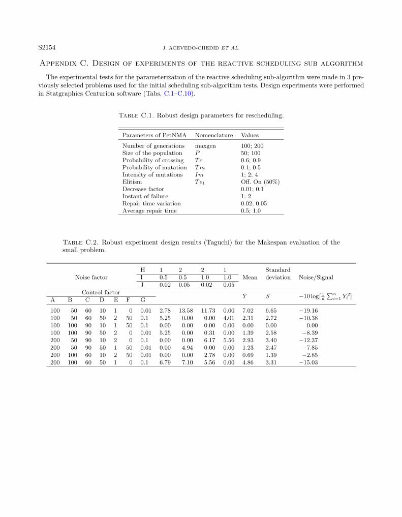
S2154 J. ACEVEDO-CHEDID ET AL.
Appendix C. Design of experiments of the reactive scheduling sub algorithm
The experimental tests for the parameterization of the reactive scheduling sub-algorithm were made in 3 pre-viously selected problems used for the initial scheduling sub-algorithm tests. Design experiments were performedin Statgraphics Centurion software (Tabs. C.1–C.10).
Table C.1. Robust design parameters for rescheduling.
Parameters of PetNMA Nomenclature Values
Number of generations maxgen 100; 200Size of the population P 50; 100Probability of crossing Tc 0.6; 0.9Probability of mutation Tm 0.1; 0.5Intensity of mutations Im 1; 2; 4Elitism Te1 Off. On (50%)Decrease factor 0.01; 0.1Instant of failure 1; 2Repair time variation 0.02; 0.05Average repair time 0.5; 1.0
Table C.2. Robust experiment design results (Taguchi) for the Makespan evaluation of thesmall problem.
H 1 2 2 1 StandardNoise factor I 0.5 0.5 1.0 1.0 Mean deviation Noise/Signal
J 0.02 0.05 0.02 0.05
Control factorY S −10 log[ 1
n
∑ni=1 Y 2
i ]A B C D E F G
100 50 60 10 1 0 0.01 2.78 13.58 11.73 0.00 7.02 6.65 −19.16100 50 60 50 2 50 0.1 5.25 0.00 0.00 4.01 2.31 2.72 −10.38100 100 90 10 1 50 0.1 0.00 0.00 0.00 0.00 0.00 0.00 0.00100 100 90 50 2 0 0.01 5.25 0.00 0.31 0.00 1.39 2.58 −8.39200 50 90 10 2 0 0.1 0.00 0.00 6.17 5.56 2.93 3.40 −12.37200 50 90 50 1 50 0.01 0.00 4.94 0.00 0.00 1.23 2.47 −7.85200 100 60 10 2 50 0.01 0.00 0.00 2.78 0.00 0.69 1.39 −2.85200 100 60 50 1 0 0.1 6.79 7.10 5.56 0.00 4.86 3.31 −15.03

SOFT-COMPUTING APPROACHES FOR RESCHEDULING PROBLEMS IN A MANUFACTURING INDUSTRY S2155
Table C.3. Robust experiment design results (Taguchi) for the Makespan evaluation of themedium problem.
H 1 2 2 1 StandardNoise factor I 0.5 0.5 1.0 1.0 Mean deviation Noise/Signal
J 0.02 0.05 0.02 0.05
Control factorY S −10 log[ 1
n
∑ni=1 Y 2
i ]A B C D E F G
100 50 60 10 1 0 0.01 9.08 7.06 0.00 6.18 5.58 3.91 −16.30100 50 60 50 2 50 0.1 14.39 0.00 13.35 4.41 8.04 6.98 −20.05100 100 90 10 1 50 0.1 9.58 0.00 2.92 12.07 6.14 5.63 −17.89100 100 90 50 2 0 0.01 1.98 0.30 0.00 0.50 0.69 0.88 −0.26200 50 90 10 2 0 0.1 7.37 0.00 0.00 0.00 1.84 3.68 −11.33200 50 90 50 1 50 0.01 7.92 2.93 1.98 7.65 5.12 3.11 −15.24200 100 60 10 2 50 0.01 0.98 6.08 4.86 2.80 3.68 2.25 −12.39200 100 60 50 1 0 0.1 13.06 0.00 7.28 0.00 5.09 6.33 −17.48
Table C.4. Robust experiment design results (Taguchi) for the Makespan evaluation of thebig problem.
H 1 2 2 1 StandardNoise factor I 0.5 0.5 1.0 1.0 Mean deviation Noise/Signal
J 0.02 0.05 0.02 0.05
Control factorY S −10 log[ 1
n
∑ni=1 Y 2
i ]A B C D E F G
100 50 60 10 1 0 0.01 2.37 7.87 6.69 1.97 4.73 3.00 −14.63100 50 60 50 2 50 0.1 5.20 3.59 9.45 4.00 5.56 2.68 −15.60100 100 90 10 1 50 0.1 1.60 14.96 2.36 5.14 6.02 6.15 −18.10100 100 90 50 2 0 0.01 4.02 16.54 12.20 3.92 9.17 6.26 −20.55200 50 90 10 2 0 0.1 6.30 0.00 15.75 9.84 7.97 6.59 −19.83200 50 90 50 1 50 0.01 7.48 16.21 9.84 2.36 8.97 5.74 −20.22200 100 60 10 2 50 0.01 4.33 3.15 9.88 2.39 4.94 3.39 −15.19200 100 60 50 1 0 0.1 3.60 11.76 14.57 1.97 7.98 6.14 −19.63
Table C.5. Robust experiment design results (Taguchi) for the TWT evaluation of the smallproblem.
H 1 2 2 1 StandardNoise factor I 0.5 0.5 1.0 1.0 Mean deviation Noise/Signal
J 0.02 0.05 0.02 0.05Control factor
Y S −10 log[ 1n
∑ni=1 Y 2
i ]A B C D E F G
100 50 60 50 4 50 0.1 0.00 0.00 0.00 0.00 0.00 0.00 0.00100 100 90 10 2 50 0.1 0.00 0.00 0.00 0.00 0.00 0.00 0.00100 100 90 50 4 0 0.01 0.00 0.00 0.00 0.00 0.00 0.00 0.00200 50 90 10 4 0 0.1 0.00 0.00 0.00 0.00 0.00 0.00 0.00200 50 90 50 2 50 0.01 0.00 0.00 0.00 0.00 0.00 0.00 0.00200 100 60 10 4 50 0.01 0.00 0.00 0.00 0.00 0.00 0.00 0.00200 100 60 50 2 0 0.1 0.00 0.00 0.00 0.00 0.00 0.00 0.00

S2156 J. ACEVEDO-CHEDID ET AL.
Table C.6. Robust experiment design results (Taguchi) for the TWT evaluation of the mediumproblem.
H 1 2 2 1 StandardNoise factor I 0.5 0.5 1.0 1.0 Mean deviation Noise/Signal
J 0.02 0.05 0.02 0.05
Control factorY S −10 log[ 1
n
∑ni=1 Y 2
i ]A B C D E F G
100 50 60 10 2 0 0.01 110.43 0.00 16.23 161.63 72.07 77.04 −39.84100 50 60 50 4 50 0.1 45.18 8.36 49.06 110.59 53.30 42.37 −36.22100 100 90 10 2 50 0.1 −3.07 47.11 7.35 235.01 71.60 111.06 −41.58100 100 90 50 4 0 0.01 50.00 5.63 67.22 33.11 38.99 26.24 −33.09200 50 90 10 4 0 0.1 120.65 16.73 0.00 79.87 54.31 56.02 −37.25200 50 90 50 2 50 0.01 64.53 8.62 5.81 94.22 43.30 43.40 −35.17200 100 60 10 4 50 0.01 30.47 0.55 3.75 99.67 33.61 46.04 −34.34200 100 60 50 2 0 0.1 55.17 50.08 4.82 0.00 27.52 29.13 −31.44
Table C.7. Robust experiment design results (Taguchi) for the TWT evaluation of the bigproblem.
H 1 2 2 1 StandardNoise factor I 0.5 0.5 1.0 1.0 Mean deviation Noise/Signal
J 0.02 0.05 0.02 0.05
Control factorY S −10 log[ 1
n
∑ni=1 Y 2
i ]A B C D E F G
100 50 60 10 2 0 0.01 2100 0 0 2100 1050.00 1212.44 −63.43100 50 60 50 4 50 0.1 8100 3300 8400 7500 6825.00 2379.60 −77.06100 100 90 10 2 50 0.1 2100 0 5100 3900 2775.00 2223.17 −70.57100 100 90 50 4 0 0.01 0 5400 0 4700 2525.00 2929.59 −71.08200 50 90 10 4 0 0.1 0 0 0 1300 325.00 650.00 −56.26200 50 90 50 2 50 0.01 0 0 0 0 0.00 0.00 0.00200 100 60 10 4 50 0.01 11400 0 6000 2100 4875.00 5010.24 −76.29200 100 60 50 2 0 0.1 100 0 600 1200 475.00 550.00 −56.56
Table C.8. Robust experiment design results (Taguchi) for the Weighted Objective evaluationof the Small problem.
H 1 2 2 1 StandardNoise factor I 0.5 0.5 1.0 1.0 Mean deviation Noise/Signal
J 0.02 0.05 0.02 0.05
Control factorY S −10 log[ 1
n
∑ni=1 Y 2
i ]A B C D E F G
100 50 60 10 2 0 0.01 0.00 12.65 11.42 4.32 7.10 5.99 −18.88100 50 60 50 4 50 0.1 4.32 2.16 10.49 0.00 4.24 4.52 −15.23100 100 90 10 2 50 0.1 0.00 0.00 12.65 0.00 3.16 6.33 −16.02100 100 90 50 4 0 0.01 0.00 13.89 3.09 0.00 4.24 6.59 −17.04200 50 90 10 4 0 0.1 0.00 0.00 0.00 3.09 0.77 1.54 −3.77200 50 90 50 2 50 0.01 5.25 0.00 1.54 8.33 3.78 3.75 −13.95200 100 60 10 4 50 0.01 0.00 0.00 12.65 0.00 3.16 6.33 −16.02200 100 60 50 2 0 0.1 0.00 13.89 3.09 0.00 4.24 6.59 −17.04

SOFT-COMPUTING APPROACHES FOR RESCHEDULING PROBLEMS IN A MANUFACTURING INDUSTRY S2157
Table C.9. Robust experiment design results (Taguchi) for the Weighted Objective evaluationof the Medium problem.
H 1 2 2 1 StandardNoise factor I 0.5 0.5 1.0 1.0 Mean deviation Noise/Signal
J 0.02 0.05 0.02 0.05
Control factorY S −10 log[ 1
n
∑ni=1 Y 2
i ]A B C D E F G
100 50 60 10 2 0 0.01 11.28 1.31 4.36 87.61 26.14 41.19 −32.91100 50 60 50 4 50 0.1 50.15 11.33 40.96 12.54 28.74 19.77 −30.49100 100 90 10 2 50 0.1 30.15 0.45 1.73 30.69 15.75 16.94 −26.66100 100 90 50 4 0 0.01 22.63 11.48 3.95 5.61 10.92 8.45 −22.37200 50 90 10 4 0 0.1 11.74 56.55 48.13 9.88 31.58 24.24 −31.58200 50 90 50 2 50 0.01 5.50 9.69 25.80 32.86 18.46 12.99 −26.70200 100 60 10 4 50 0.01 90.57 4.24 0.00 20.81 28.90 42.08 −33.35200 100 60 50 2 0 0.1 33.86 31.67 5.06 107.44 44.51 43.95 −35.35
Table C.10. Robust experiment design results (Taguchi) for the Weighted Objective evaluationof the Big problem.
H 1 2 2 1 StandardNoise factor I 0.5 0.5 1.0 1.0 Mean deviation Noise/Signal
J 0.02 0.05 0.02 0.05
Control factorY S −10 log[ 1
n
∑ni=1 Y 2
i ]A B C D E F G
100 50 60 10 1 0 0.01 1.95 0.00 17.51 44.92 16.10 20.75 −27.65100 50 60 50 4 50 0.1 7.03 7.00 12.11 145.70 42.96 68.54 −37.30100 100 90 10 1 50 0.1 21.40 0.00 0.00 69.14 22.64 32.60 −31.17100 100 90 50 4 0 0.01 27.48 61.87 20.70 147.27 64.33 58.15 −38.24200 50 90 10 4 0 0.1 27.13 9.38 17.69 39.45 23.41 12.92 −28.28200 50 90 50 1 50 0.01 14.84 1.56 20.70 1.56 9.67 9.66 −22.13200 100 60 10 4 50 0.01 43.58 15.23 2.34 7.42 17.14 18.40 −27.39200 100 60 50 1 0 0.1 22.27 0.00 3.83 24.22 12.58 12.44 −24.38
References
[1] J. Acevedo and G. Mejıa, Programacion reactiva y robusta de la produccion en un ambiente sistema de manufactura flexible:llegada de nuevas ordenes y cambios en la prioridad de las ordenes de trabajo. Maestria, Departamento de Ingenierıa Industrial,Universidad de los Andes (2006).
[2] N. Al-Hinai and T. El-Mekkawy, An efficient hybridized genetic algorithm architecture for the flexible job shop schedulingproblem. Flexible Serv. Manuf. J. 23 (2011) 64–85.
[3] O. Basak and Y.E. Albayrak, Petri net based decision system modeling in real-time scheduling and control of flexible automotivemanufacturing systems. Comput. Ind. Eng. 86 (2015) 116–126.
[4] O.T. Baruwa, M.A. Piera and A. Guasch, Deadlock-free scheduling method for flexible manufacturing systems based on timedcolored Petri nets and anytime heuristic search. IEEE Trans. Syst. Man Cybern. 45 (2014) 831–846.
[5] J.A. Chedid, K.S. Navarro, H.O. Mateus and A.S. Mercado, Reprogramacion de produccion en cadenas de suministro colabo-rativas: Una revision de la literatura. Espacio 38 (2017) 23.
[6] F. Chen and J. Chen, Performance modelling and evaluation of dynamic tool allocation in flexible manufacturing systemsusing coloured Petri nets: an object-oriented approach. Int. J. Adv. Manuf. Technol. 21 (2003) 98–109.
[7] J. Chen and F.F. Chen, Adaptive scheduling in random flexible manufacturing systems subject to machine breakdowns. Int.J. Prod. Res. 41 (2003) 1927–1951.
[8] H. Cho, Petri net models for message manipulation and event monitoring in an FMS cell. Int. J. Prod. Res. 36 (1998) 231–250.
[9] C. Cotta, L. Mathieson and P. Moscato, Memetic algorithms. In: Handbook of Heuristics edited by R. Martı, P. M. Pardalos,M. G. C. Resende. Springer, Cham (2018) 607–638.

S2158 J. ACEVEDO-CHEDID ET AL.
[10] B.K. Dey, S. Pareek, M. Tayyab and B. Sarkar, Autonomation policy to control work-in-process inventory in a smart productionsystem. Int. J. Prod. Res. (2020) 1–23. DOI: 10.1080/00207543.2020.1722325.
[11] J. Dorn, R. Kerr and G. Thalhammer, Reactive scheduling: improving the robustness of schedules and restricting the effectsof shop floor disturbances by fuzzy reasoning. Int. J. Human-Comput. Stud. 42 (1995) 687–704.
[12] H.A. Elmaraghy and T.Y. Elmekkawy, Deadlock-free rescheduling in flexible manufacturing systems. CIRP Ann. 51 (2002)371–374.
[13] M.R. Garey, D.S. Johnson and R. Sethi, The complexity of flowshop and jobshop scheduling. Math. Oper. Res. 1 (1976) 117–129.
[14] P. Garg, A comparison between Memetic algorithm and Genetic algorithm for the cryptanalysis of simplified data encryptionstandard algorithm. Int. J. Network Secur. App. 1 (2009) 34–42.
[15] A. Gholami, R. Sheikh, N. Mizani and S.S. Sana, ABC analysis of the customers using axiomatic design and incomplete roughset. RAIRO:OR 52 (2018) 1219–1232.
[16] R. Guchhait, B.K. Dey, S. Bhuniya, B. Ganguly, B. Mandal, R.K. Bachar, B. Sarkar, H.M. Wee and K. Chaudhuri, Invest-ment for process quality improvement and setup cost reduction in an imperfect production process with warranty policy andshortages. RAIRO:OR 54 (2020) 251–266.
[17] L. Han, K. Xing, X. Chen, H. Lei and F. Wang, Deadlock-free genetic scheduling for flexible manufacturing systems usingPetri nets and deadlock controllers. Int. J. Prod. Res. 52 (2014) 1557-1572.
[18] L. Han, K. Xing, X. Chen and F. Xiong, A Petri net-based particle swarm optimization approach for scheduling deadlock-proneflexible manufacturing systems. J. Intel. Manuf. 29 (2018) 1083–1096.
[19] S.K. Hasan, R. Sarker and D. Essam, Genetic algorithm for job-shop scheduling with machine unavailability and breakdowns.Int. J. Prod. Res. 49 (2011) 4999–5015.
[20] I. Hatono, K. Yamagata and H. Tamura, Modeling and online scheduling of flexible manufacturing systems using stochasticPetri nets. IEEE Trans. Softw. Eng. 17 (1991) 126–132.
[21] H. Hoos and T. Stutzle, Stochastic Local Search: Foundations and Applications. Morgan Kaufmann Publishers, San Francisco,CA (2005).
[22] B. Huang, Z. Cai, M. Zhou and J. Hao, Scheduling of FMS based on binary decision diagram and Petri net. In: IEEE 15thInternational Conference on Networking, Sensing and Control (ICNSC). (2018) 1–6.
[23] G. Jamali, S.S. Sana and R. Moghdani, Hybrid improved cuckoo search algorithm and genetic algorithm for solving markov-modulated demand. RAIRO:OR 52 (2018) 473–497.
[24] A. Khanna, P. Gautam, B. Sarkar and C.K. Jaggi, Integrated vendor–buyer strategies for imperfect production systems withmaintenance and warranty policy. RAIRO:OR 54 (2020) 435–450.
[25] Y.W. Kim, T. Suzuki and T. Narikiyo, FMS scheduling based on timed Petri Net model and reactive graph search. Appl.Math. Modell. 31 (2007) 955–970.
[26] S. Kirkpatrick, C.D. Gelatt and M.P. Vecchi, Optimization by simulated annealing. Science 220 (1983) 671–680.
[27] R.R. Kumar, A.K. Singh and M. Tiwari, A fuzzy based algorithm to solve the machine-loading problems of a FMS and itsneuro fuzzy Petri net model. Int. J. Adv. Manuf. Technol. 23 (2004) 318–341.
[28] B.S. Kumar, G.J. Raju and G.R. Janardhana, Production planning in flexible manufacturing system by considering the multi-objective functions. In: Advances in Materials and Manufacturing Engineering. Lecture Notes in Mechanical Engineering.(ICAMME 2019) Springer, Singapore (2020) 343–352.
[29] H. Lei, K. Xing, L. Han and Z. Gao, Hybrid heuristic search approach for deadlock-free scheduling of flexible manufacturingsystems using Petri nets. Appl. Soft Comput. 55 (2017) 413–423.
[30] C. Li, W. Wu, Y. Feng and G. Rong, Scheduling FMS problems with heuristic search function and transition-timed Petri nets.J. Intell. Manuf. 26 (2015) 933–944.
[31] C. Low and T.H. Wu, Mathematical modelling and heuristic approaches to operation scheduling problems in an FMS environ-ment. Int. Jo. Prod. Res. 39 (2001) 689–708.
[32] D.R. Mahapatra, S. Panda and S.S. Sana, Multi-choice and stochastic programming for transportation problem involved insupply of foods and medicines to hospitals with consideration of logistic distribution. RAIRO:OR 54 (2020) 1119–1132.
[33] S.V. Mehta, Predictable scheduling of a single machine subject to breakdowns. Int. J. Comput. Integr. Manuf. 12 (1999) 15–38.
[34] G. Mejia and J. Acevedo, Reactive scheduling in FMS: an integrated approach based on petri nets, genetic algorithms andsimulation. In: Third International Conference on Production Research, Americas’ Region (2006).
[35] G. Mejıa and K. Nino, A new Hybrid Filtered Beam Search algorithm for deadlock-free scheduling of flexible manufacturingsystems using Petri Nets. Comput. Ind. Eng. 108 (2017) 165–176.
[36] U. Mishra, J.Z. Wu and B. Sarkar, A sustainable production-inventory model for a controllable carbon emissions rate undershortages. J. Cleaner Prod. 256 (2020) 120268.
[37] P. Moscato and C. Cotta, Una introduccion a los algoritmos memeticos. Intel. Artif. Rev. Iberoamericana Intel. Artif. 7 (2003)131–148.
[38] T. Murata, Petri nets: properties, analysis and applications. Proc. IEEE 77 (1989) 541–580.
[39] H.Z. Nabi and T. Aized, Performance evaluation of a carousel configured multiple products flexible manufacturing systemusing Petri net. Oper. Manag. Res. 13 (2020) 109–129.
[40] K.S. Navarro, J.A. Chedid, G.M. Arquez, W.F. Florez, H.O. Mateus, S.S. Sana and L.E. Cardenas-Barron, An EPQ inventorymodel considering an imperfect production system with probabilistic demand and collaborative approach. J. Adv. Manage.Res. 17 (2019) 282–304.

SOFT-COMPUTING APPROACHES FOR RESCHEDULING PROBLEMS IN A MANUFACTURING INDUSTRY S2159
[41] K.S. Navarro, J.A. Chedid, W.F. Florez, H.O. Mateus, L.E. Cardenas-Barron and S.S. Sana, A collaborative EPQ inventorymodel for a three-echelon supply chain with multiple products considering the effect of marketing effort on demand. J. Ind.Manage. Optim. 16 (2020) 1613–1633.
[42] P.S. Pachpor, R. Shrivastava, D. Seth and S. Pokharel, Application of Petri nets towards improved utilization of machines injob shop manufacturing environments. J. Manuf. Technol. Manage. 28 (2017) 169–188.
[43] A.M. Patel and A.Y. Joshi, Modeling and analysis of a manufacturing system with deadlocks to generate the reachability treeusing Petri net system. Proc. Eng. 64 (2013) 775–784.
[44] M. Pinedo, Scheduling. Springer, Cham (2012).
[45] M. Pinedo, Planning and Scheduling in Manufacturing and Services. Springer, New York, NY (2005).
[46] S.S. Sana, H. Ospina-Mateus, F.G. Arrieta and J.A. Chedid, Application of genetic algorithm to job scheduling under ergonomicconstraints in manufacturing industry. J. Ambient Intell. Humanized Comput. 10 (2019) 2063–2090.
[47] S.S. Sankar, S. Ponnanbalam and C. Rajendran, A multiobjective genetic algorithm for scheduling a flexible manufacturingsystem. Int. J. Adv. Manuf. Technol. 22 (2003) 229–236.
[48] S.S. Sankar, S. Ponnambalam and M. Gurumarimuthu, Scheduling flexible manufacturing systems using parallelization ofmulti-objective evolutionary algorithms. Int. J. Adv. Manuf. Technol. 30 (2006) 279–285.
[49] B. Santosa, R. Damayanti and B. Sarkar, Solving multi-product inventory ship routing with a heterogeneous fleet model usinga hybrid cross entropy-genetic algorithm: a case study in Indonesia Prod. Manuf. Res. 4 (2016) 90–113.
[50] N. Saxena, B. Sarkar and S. Singh, Selection of remanufacturing/production cycles with an alternative market: a perspectiveon waste management. J. Cleaner Prod. 245 (2020) 118935.
[51] B.K. Sett, S. Sarkar and B. Sarkar, Optimal buffer inventory and inspection errors in an imperfect production system withpreventive maintenance. Int. J. Adv. Manuf. Technol. 90 (2017) 545–560.
[52] M. Souier, M. Dahane and F. Maliki, An NSGA-II-based multiobjective approach for real-time routing selection in a flexiblemanufacturing system under uncertainty and reliability constraints. Int. J. Adv. Manuf. Technol. 100 (2019) 2813–2829.
[53] A.A. Taleizadeh, L.E. Cardenas-Barron and B. Mohammadi, A deterministic multi product single machine EPQ model withbackordering, scraped products, rework and interruption in manufacturing process. Int. J. Prod. Econ. 150 (2014) 9–27.
[54] Y. Tanimizu, T. Sakaguchi, K. Iwamura and N. Sugimura, Evolutional reactive scheduling for agile manufacturing systems.Int. J. Prod. Res. 44 (2006) 3727–3742.
[55] E.S. Tashnizi, S. Farahani and A.F. Nahrekhalaji, Production process optimization in flexible manufacturing system usingPetri nets. In: Proceedings of the World Congress on Engineering and Computer Science (2008) 22–24.
[56] M. Tayyab, J. Jemai, H. Lim and B. Sarkar, A sustainable development framework for a cleaner multi-item multi-stage textileproduction system with a process improvement initiative. J. Cleaner Prod. 246 (2020) 119055.
[57] S. Tian, T. Wang, L. Zhang and X. Wu, Real-time shop floor scheduling method based on virtual queue adaptive control:algorithm and experimental results. Measurement 147 (2019) 106689.
[58] F. Tuysuz and C. Kahraman, Modeling a flexible manufacturing cell using stochastic Petri nets with fuzzy parameters. ExpertSyst. App. 37 (2010) 3910–3920.
[59] M. Ullah and B. Sarkar, Recovery-channel selection in a hybrid manufacturing-remanufacturing production model with RFIDand product quality. Int. J. Prod. Econ. 219 (2020) 360–374.
[60] G.E. Vieira, J.W. Herrmann and E. Lin, Rescheduling manufacturing systems: a framework of strategies, policies, and methods.J. Schedul. 6 (2003) 39–62.
[61] Z. Zhao, G. Zhang and Z. Bing, Scheduling optimization for FMS based on Petri net modeling and GA. In: IEEE InternationalConference on Automation and Logistics (ICAL) (2011) 422–427.