soil moisture remote sensing using gps-interferometric...
TRANSCRIPT

i
Soil Moisture Remote Sensing using GPS-Interferometric Reflectometry
by
Clara Chew
B.A., Dartmouth College, 2009
A thesis submitted to the Faculty of the Graduate School
of the University of Colorado in partial fulfillment
of the requirements for the degree of
Doctor of Philosophy
Department of Geological Sciences
2015

ii
This thesis entitled:
Soil Moisture Remote Sensing using Global Positioning System-Interferometric Reflectometry
Written by Clara C. Chew
Has been approved for the Department of Geological Sciences by:
_______________________________________________
Eric Small
________________________________________________
Kristine Larson
________________________________________________
Shemin Ge
________________________________________________
Greg Tucker
________________________________________________
Valery Zavorotny
Date: ________________________
The final copy of this thesis has been examined by the signatories, and we find that both the
content and the form meet acceptable presentation standards of scholarly work in the above
mentioned discipline.

iii
Clara C. Chew
Soil moisture remote sensing using Global Positioning System-Interferometric Reflectometry
Thesis directed by Prof. Eric Small
Ground-reflected Global Positioning System (GPS) signals can be used opportunistically
to infer changes in land-surface characteristics surrounding a GPS monument. GPS satellites
transmit at L-band, and at microwave frequencies the permittivity of the ground surface changes
primarily due to its moisture content. Temporal changes in ground-reflected GPS signals are thus
indicative of temporal changes in the moisture content surrounding a GPS antenna.
The interference pattern of the direct and reflected GPS signal for a single satellite track
is recorded in signal-to-noise ratio (SNR) data. Alternating constructive and destructive
interference as the satellite passes over the antenna results in a noisy oscillating wave at low
satellite elevation angles, from which the phase, amplitude, and frequency (or reflector height)
can be calculated.
Here, an electrodynamic model that simulates SNR data is validated against field
observations. The model is then used to show that temporal changes in these SNR metrics may
be used to estimate changes in surface soil moisture in the top 5 cm of the soil column. Results
show that changes in SNR phase are best correlated with changes in soil moisture, with an
approximately linear slope. Surface roughness decreases the sensitivity of SNR phase to soil
moisture, though the effect is not significant for small roughness values (<5 cm).
Modeling experiments show that all three SNR metrics are affected by changes in the
permittivity and height of a vegetation canopy. SNR amplitude is the best indicator of changes in
vegetation. An increase in either canopy permittivity or height will cause a corresponding
decrease in SNR phase. Seasonal changes in vegetation must be removed if soil moisture is to be
estimated using phase data.
An algorithm is presented that uses modeled relationships between canopy parameters
and SNR metrics to remove seasonal vegetation effects from the phase time series, from which
soil moisture time series may be estimated. Results indicate that this algorithm can successfully
estimate surface soil moisture with an RMSE of 0.05 cm3
cm-3
or lower for many of the antennas
that comprise the Plate Boundary Observatory (PBO) network.

iv
Acknowledgements
Five years ago, Eric Small made the strange decision to allow me to work in the GPS
reflections group. I often look back to this time of my life and wonder just what possessed him to
give me such an opportunity, and I have to chalk it up to serendipity. I am incredibly thankful to
him for making my graduate school experience not only fruitful, but even enjoyable. He has
always done his best to keep me thinking about the big picture, which has kept me from falling
too deeply into numerous rabbit holes.
Along with Eric, Kristine Larson has also been an incredible advisor. Her dedication to
GPS and work ethic is inspiring, and I can only hope a little rub of this has rubbed off on me.
Her attention to detail is responsible for much of the success of the GPS reflections project, and I
am very lucky to have been able to call her my mentor.
I am also indebted to Valery Zavorotny, without whom this entire thesis would not have
been possible. His expertise in electromagnetic scattering is unparalleled, and I am certain he
could have done all the work that I did in a tenth of the time. Even so, he patiently answered all
of my questions, and always with a grin.
Next, I would like to thank Greg Tucker and Shemin Ge for serving on my committee.
They have both been very encouraging during my time here, and seeing them excel at their own
research has motivated me to work harder at mine.
I am very thankful for the opportunities I have had to work with current and past
collaborators and colleagues—John Braun, Andria Bilich, Felipe Nievinski, Sarah Evans, Peter
Shellito, Karen Boniface, James McCreight, John Pratt, Evan Pugh, Tevis Blom, Shahen Huda,
Maria Rocco, and Cheney Shreve. Thank you for the support you have given, insightful
conversations we have had, and the fieldwork we have shared.
This research would not have been possible without the support of funding from the
University of Colorado, NASA, and NSF.

v
Table of Contents
Acknowledgements ...................................................................................................................................... iv
List of Figures ............................................................................................................................................ viii
List of Tables .............................................................................................................................................. xii
Chapter 1: Introduction ................................................................................................................................. 1
Chapter 2: Background ................................................................................................................................. 3
2.1 Soil moisture measurement ................................................................................................................. 3
2.2 Soil moisture variability ...................................................................................................................... 6
2.3 The Plate Boundary Observatory Network ......................................................................................... 7
2.4 Remote sensing using GPS reflected signals ...................................................................................... 8
2.5 GPS-Interferometric Reflectometry .................................................................................................... 9
2.6 Signal-to-Noise Ratio Data ............................................................................................................... 12
2.6.1 SNR Equation and metrics ......................................................................................................... 12
2.6.2 Temporal changes in SNR metrics ............................................................................................. 15
Chapter 3: Ground truth experiments and data ........................................................................................... 18
3.1 Description of measurement techniques ........................................................................................... 18
3.1.1 In situ soil moisture data ............................................................................................................ 18
3.1.2 Vegetation surveys ..................................................................................................................... 21
3.2 Data Summary .................................................................................................................................. 21
3.2.1 Soil Moisture Data ..................................................................................................................... 21
3.2.2 Vegetation Data.......................................................................................................................... 24
Chapter 4: Forward modeling of SNR data in relation to soil moisture and vegetation ............................. 27
4.1 Model architecture ............................................................................................................................ 28
4.1.1 Reflection coefficient calculations ............................................................................................. 28
4.1.2 Permittivity profile generation: Soil .......................................................................................... 30
4.1.3 Permittivity profile generation: Vegetation ............................................................................... 31
4.1.4 Note on the plane-stratified model for a vegetation canopy ...................................................... 35
4.1.5 Calculation of direct and indirect power .................................................................................... 36
4.2 Model validation ............................................................................................................................... 38
4.2.1 Validation Set-Up: Field Observations and Model Input .......................................................... 38
4.2.2 Comparison of Simulated and Observed SNR Data .................................................................. 40
4.2.3 Comparison of Simulated SNR and Observed Metrics .............................................................. 43
4.3 Bare Soil Modeling ........................................................................................................................... 46

vi
4.3.1 Soil moisture profiles ................................................................................................................. 46
4.3.2 Modeled SNR interferograms .................................................................................................... 48
4.3.3 The effect of soil moisture on SNR metrics ............................................................................... 50
4.4 Vegetation-soil model ....................................................................................................................... 55
4.4.1 First case: random combinations of vegetation parameters ....................................................... 57
4.4.2 Second case: Assuming relationships between canopy parameters ........................................... 66
4.4.3 Third case: When specific vegetation parameters are correlated with one another ................... 69
4.4.4 Effects of underlying soil moisture changes .............................................................................. 71
4.4.5 Problems with the constant-frequency SNR equation ............................................................... 76
4.4.6 Conclusions ................................................................................................................................ 77
Chapter 5: Correcting for vegetation effects on SNR data ......................................................................... 79
5.1 Extent of vegetation effects in observed data ................................................................................... 79
5.2 Development of the vegetation filter ................................................................................................ 80
5.2.1 SNR model simulations ............................................................................................................. 81
5.2.2 Relationships between SNR metrics .......................................................................................... 82
5.3 Processing observed SNR metrics .................................................................................................... 83
5.4 Estimating phase change due to vegetation ...................................................................................... 84
5.5 Justification for the current filter ...................................................................................................... 87
5.5.1 Concurrent inverse estimation of soil moisture and vegetation ................................................. 87
5.5.2 The use of a more complex characteristic SNR equation .......................................................... 91
5.6 Limitations of the vegetation filter .................................................................................................... 93
Chapter 6: Soil Moisture Estimations using GPS-IR .................................................................................. 97
6.1 Empirical data issues ......................................................................................................................... 97
6.1.1 Persistent amplitude anomalies .................................................................................................. 97
6.1.2 Reflector height considerations ................................................................................................ 101
6.2 Soil moisture retrieval algorithm .................................................................................................... 115
6.3 Validation of soil moisture retrievals .............................................................................................. 127
6.4 Effect of changing model parameters ............................................................................................. 129
6.4.1 Sensitivity to changing the a priori reflector height ................................................................ 131
6.4.2 Sensitivity to changes in the smoothing method ...................................................................... 133
Chapter 7: Error Quantification ................................................................................................................ 135
7.1 Errors for bare soil .......................................................................................................................... 135
7.1.1 Imperfect knowledge of a priori reflector height .................................................................... 135

vii
7.1.2 Vertical gradients in SMC profiles .......................................................................................... 137
7.1.3 Differences in antenna height .................................................................................................. 139
7.1.4 Differences in soil texture ........................................................................................................ 140
7.1.5 Changes in soil temperature ..................................................................................................... 141
7.1.6 Changes in receiver temperature .............................................................................................. 142
7.1.7 Surface roughness .................................................................................................................... 143
7.2 Errors for vegetated environments .................................................................................................. 146
7.2.1 Imperfect knowledge of antenna height ................................................................................... 146
Chapter 8: Future Work ............................................................................................................................ 150
8.1 Improvements in model simulations for the vegetation filter ......................................................... 150
8.2 Improvements in quality control of observations............................................................................ 153
Chapter 9: Conclusions ............................................................................................................................. 156
Bibliography ............................................................................................................................................. 158

viii
List of Figures
Figure 1: Locations of selected PBO GPS sites that are currently being used to estimate soil
moisture.
Figure 2: Geometry of a multipath signal.
Figure 3: Plan view diagrams for the GPS station okl3.
Figure 4: Examples of SNR interferograms.
Figure 5: Examples of SNR metric time series.
Figure 6: Distributions of in situ soil moisture at the validation sites.
Figure 7: Relationships between vegetation field measurements.
Figure 8: Vegetation-soil model schematic.
Figure 9: Validation of the model with observed SNR interferograms.
Figure 10: Comparison between observed and modeled SNR metrics at the alfalfa field.
Figure 11: Validation of the soil-vegetation model against observed SNR metrics.
Figure 12: Modeled relationships between SNR metrics and soil moisture, for a bare soil.
Figure 13: Model simulations and observed data from a wheat field.
Figure 14: Modeled interferograms for a bare soil.
Figure 15: Modeled normalized amplitude and soil moisture, and modeled change in effective
reflector height, for a bare soil.
Figure 16: Observed vegetation data and SNR metrics for a GPS station in Oklahoma.
Figure 17: Modeled relationships between dry biomass and SNR metrics.
Figure 18: Modeled relationships between vegetation wet weight and SNR metrics.
Figure 19: Modeled relationships between canopy height and SNR metrics.
Figure 20: Modeled relationships between vegetation true density and SNR metrics.
Figure 21: Relationships between modeled canopy permittivity, height, and SNR metrics.
Figure 22: Examples of observed changes in Lomb-Scargle Periodograms throughout the
growing season.
Figure 23: Vegetation field data comparison between a desert steppe and alfalfa site.

ix
Figure 24: Modeled relationships between vegetation wet weight and SNR metrics, for typical
vegetation present at the desert steppe and alfalfa sites.
Figure 25: Modeled relationships between vegetation wet weight and SNR metrics, when
vegetation true density is pinned to water content.
Figure 26: Sensitivity of SNR metrics to changes in soil moisture underlying modeled vegetation
canopies.
Figure 27: Characterization of the misfit between interferograms and their associated metrics.
Figure 28: The fraction of PBO H2O data that is likely affected by vegetation.
Figure 29: Distributions of vegetation parameters used in the vegetation filter.
Figure 30: Relationships between SNR metrics and phase, given changes in modeled vegetation
canopies.
Figure 31: Relationships between multiple SNR metrics and phase, given changes in modeled
vegetation canopies.
Figure 32: SNR metrics for multiple satellite tracks at a GPS site in Oklahoma.
Figure 33: Estimated versus observed canopy height at the alfalfa site, bcgr.
Figure 35: Depiction of how the vegetation filter would change, given soil moisture change.
Figure 34: Modeled reflection coefficients for example vegetation canopies.
Figure 36: Modeled interferograms and SNR metrics for a theoretical, isotropic antenna.
Figure 37: Examples of observed amplitude anomalies.
Figure 38: Amplitude time series for one satellite track at a GPS site in Oklahoma.
Figure 39: Depiction of the tolerance limits for determining systemic amplitude problems.
Figure 40: Time series of normalized LSP amplitude data for several satellite tracks and the
tolerance limits.
Figure 41: Time series of effective reflector height for one satellite track at the desert steppe site
p041.
Figure 42: Time series of estimated soil moisture at site p041, before and after a flooding event.
Figure 43: Estimated and in situ soil moisture data from p041 at the beginning of 2012.
Figure 44: The effect of using an incorrect a priori reflector height on phase and amplitude.

x
Figure 45: Time series of effective reflector heights at p041, and phase time series before and
after reflector height correction.
Figure 46: Comparison of estimated soil moisture time series at p041, with and without a
reflector height correction.
Figure 47: Modeled relationships between canopy height and effective reflector height.
Figure 48: Examples of the current a priori reflector heights versus the median value of the
effective reflector height.
Figure 49: Effects of changing the a priori reflector height on soil moisture retrievals.
Figure 50: Digital elevation model and ground tracks at the GPS site okl3.
Figure 51: Histogram of the number of satellite tracks used at PBO H2O stations and an example
of the track number increasing at a site over time.
Figure 53: Soil moisture retrieval algorithm flowchart.
Figure 52: Soil moisture retrievals and in situ data from a desert steppe site mfle.
Figure 54: Soil moisture retrievals with and without using the vegetation filter at GPS site okl3.
Figure 55: A soil pit in Oklahoma and measurements from three different types of in situ soil
moisture probes.
Figure 56: Validation plot showing GPS versus in situ soil moisture estimations.
Figure 57: Examples of how changing the a priori height at ames changes results from the
vegetation filter.
Figure 58: Examples of how the choice of smoothing parameters affects the outcome of the
vegetation filter.
Figure 59: Modeled errors in soil moisture retrievals from a priori reflector height errors.
Figure 60: Errors introduced from vertical gradients in soil moisture profiles.
Figure 61: Errors introduced from using data from antennas of different heights.
Figure 62: Differences in the relationship between soil moisture and phase for different soil
textures.
Figure 63: Effect of ground temperature on phase and amplitude.
Figure 64: Observed effects of temperature on SNR metrics.

xi
Figure 65: The effect of surface roughness on the relationships between soil moisture and SNR
metrics.
Figure 66: The RMS error between surface roughness and subsequent soil moisture estimations.
Figure 67: Errors in estimated phase change due to vegetation, if the a priori reflector height is
over- or under-estimated.
Figure 68: Phase observations and predictions using two versions of the vegetation filter at p042.
Figure 69: Estimated soil moisture time series for masw using two versions of the vegetation
filter.
Figure 70: Time series of track-by-track soil moisture retrievals and in situ data at okl3.

xii
List of Tables
Table 1: Historical and current satellite missions with observations of soil moisture.
Table 2: Summary of theta probe and volumetric soil moisture surveys.
Table 3: GPS stations, antenna heights, and vegetation information.
Table 4: Mean Cross-Correlation Coefficients
Table 5: Slopes and r2 values for linear regressions of soil moisture and phase.
Table 6: Parameters used in the soil-vegetation model
Table 7: Description of parameters used in the soil moisture algorithm.
1
Chapter 1: Introduction
Soil moisture has long been recognized as an important hydrologic variable, as it
determines the relative partitioning between the turbulent sensible and latent heat fluxes [1], [2].
Soil moisture anomalies are likely to initiate positive feedback mechanisms due to the thermal
inertia of soil moisture relative to precipitation anomalies [1]. It has been shown that in areas that
lie in the transition zone between wet and dry climates, such as the Great Plains in the United
States, the Sahel, and parts of India, soil moisture and precipitation are strongly coupled. In these
areas, persistent soil moisture anomalies are likely to influence precipitation [3]. Better
initialization of soil moisture will lead to better predictive skill in numerical weather forecasts
and global climate models [3].
Currently, there is a paucity of soil moisture observations at all spatial and temporal
scales that would be needed to initialize models or validate soil moisture products. In particular,
there are few methods of soil moisture measurement or estimation that yield data on the field
scale (~1000 m2). Direct soil moisture measurement using either soil gravimetry or
electromagnetic probes yield measurements for small volumes of soil (<1 m3) [4], and remotely
sensed products from satellites have resolutions of many square kilometers [5]. Methods that do
exist for field-scale soil moisture measurement, such as instruments mounted on truck booms or
flown on aircraft, are usually used in field campaigns and not for long-term data collection.
In recent years, Global Positioning System (GPS) multipath signals have been used
opportunistically to infer land surface characteristics, such as snow depth, soil moisture, and
changes in vegetation. GPS antennas and receivers are well suited for land surface remote
sensing because the GPS satellite transmit frequency is L-band (microwave frequency) with

2
wavelengths of ~19 (L1) or 24.4 (L2) cm. Microwave remote sensing of land surface properties
has been studied for over 20 years [6]–[8]. For microwave frequencies, the permittivity or
dielectric constant of a medium is highly dependent on its water content [9]. For example, the
dielectric constant of water is around 80, compared to a dielectric constant of 3.5 for dry soils.
The permittivity of a material determines the extent to which an electromagnetic wave will
reflect off of the material, with higher permittivity materials resulting in a greater reflection [10].
As a result, the ground-reflected GPS signal will be altered by the amount of moisture
contained near the ground surface. The receiving antenna can record temporal changes in the
ground-reflected signal, which correlate with changes in properties such as soil moisture, snow,
vegetation, surface roughness, and surface temperature.
Here, I will present results pertaining to the development of a methodology for soil
moisture remote sensing using commercial GPS antennas and receivers. This work has included
adapting and validating an electrodynamic model that simulates the response of GPS ground
reflections to changes in soil moisture and vegetation canopy parameters. There is also a field
component to this research, with several years of observations made at several GPS stations that
also have concurrent soil moisture and/or vegetation observations. Using the electrodynamic
model as well as observations, I have created a soil moisture retrieval algorithm that can be used
at GPS stations with choke ring antennas, located in areas with variable vegetation cover.

3
Chapter 2: Background
2.1 Soil moisture measurement
Soil moisture in this document will always refer to volumetric soil moisture, which is the
volume of water in a soil divided by the total volume of the soil. Soil moisture content will be
abbreviated as SMC and will have units of cm3 cm
-3.
SMC varies between residual and saturated values. The residual moisture content of a soil
is always greater than zero due to the adsorption of a certain amount of water molecules to soil
grains. The residual moisture content is controlled by its soil texture, and soils with higher clay
contents will tend to have higher residual moisture contents. Typically, residual moisture
contents vary between 0.02 cm3 cm
-3 and 0.075 cm
3 cm
-3 [11]. The saturated moisture content for
a soil is equal to its porosity, or the amount of void space within the soil. Thus, a soil with a
porosity of 0.4 will also have a maximum SMC of 0.4 cm3 cm
-3.
Soil moisture is measured with both in situ and remote sensing methods. The two most
popular methods of in situ soil moisture monitoring include gravimetric/volumetric sampling and
the use of electromagnetic probes (time domain reflectometry (TDR), frequency domain
reflectometry (FDR), etc.). Volumetric sampling for volumetric water content determination
involves removing a known volume of soil and drying it to determine the mass of water lost. If
the density of water is assumed to be 1000 kg m-3
, then the volume of water present in the
original volume of soil can be determined. Gravimetric sampling is similar to volumetric
sampling, except that the technique does not require a known volume—numbers are scaled by
bulk density values. Gravimetric and volumetric surveys are time consuming, site destructive,
and are usually only conducted during field campaigns. They are also unreliable where soils are
rocky.

4
There are a variety of different kinds of electromagnetic probes, which yield
instantaneous estimations of soil moisture. Some probes may be emplaced in the ground for a
long period of time, or they may be used in short field campaigns to get point estimates of soil
moisture. TDR probes work by measuring the time it takes for an electromagnetic wave to travel
between probe rods in the soil and relating the impedance to soil moisture content [12]. FDR
probes are constructed similarly to TDR probes, but they measure the change in the frequency of
the transmitted signal, which is affected by the ground’s permittivity/moisture content.
Electromagnetic probes should be calibrated to the specific soil type for most accurate results.
Both gravimetric/volumetric and electromagnetic methods estimate soil moisture for a small
volume of soil (<1 m3) [12].
Two remote sensing methods exist for soil moisture—the use of radar or radiometers.
Radar remote sensing, also called active remote sensing, involves using an antenna to transmit
signals towards the soil surface of a specified frequency, and changes in the reflected signal are
measured by the receiving antenna. If the receiving antenna is the same as the transmitting
antenna, it is deemed monostatic radar, and if the receiving antenna is different than the
transmitting antenna, it is deemed bistatic radar. By and large the most popular method of active
radar remote sensing is using monostatic radar measurements.
Soil moisture remote sensing is typically done using either a monostatic radar or
radiometer. A monostatic radar system measures how transmitted electromagnetic waves are
attenuated by changes in soil moisture (or vegetation). Transmitted waves are reflected back to
the same transmitting antenna, and a backscatter coefficient is calculated, with higher backscatter
usually correlated with higher moisture contents [6], [13]. Monostatic radar for soil moisture
measurement, like GPS-IR, most commonly uses microwave frequencies. Radiometers differ
5
from radars in that they passively collect naturally-emitted microwave radiation from the soil.
They are able to estimate changes in moisture content due to the fact that thermal emission of
microwave radiation from soil is highly dependent on its moisture content [14].
Both monostatic radars and radiometers may be mounted on towers or truck booms [15],
flown on airplanes [16]–[18], or be mounted on satellites or spacecraft [19]. Those that are
mounted on towers or truck booms can give soil moisture estimates on the field scale, or tens to
hundreds of square meters, while those on airplanes and satellites have successively larger
sensing areas. These measurements tend to be conducted during field campaigns and do not tend
to yield long-term records. The exception to this would be instruments on satellites, such as the
Soil Moisture and Ocean Salinity (SMOS) or the recently-launched Soil Moisture Active Passive
(SMAP) satellites, which give estimates of soil moisture approximately every three days [5]. The
sensing area of spaceborne radars or radiometers is on the order of many square kilometers or
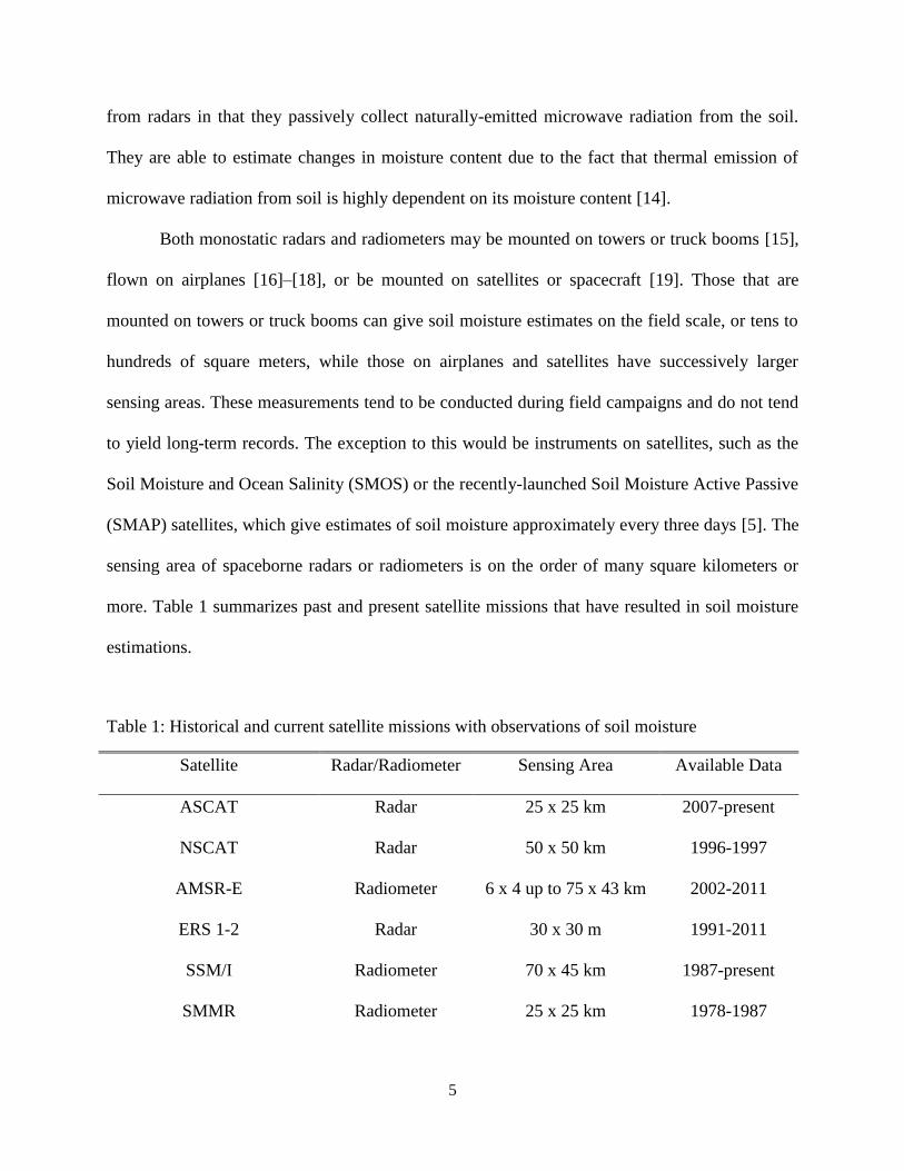
more. Table 1 summarizes past and present satellite missions that have resulted in soil moisture
estimations.
Table 1: Historical and current satellite missions with observations of soil moisture
Satellite Radar/Radiometer Sensing Area Available Data
ASCAT Radar 25 x 25 km 2007-present
NSCAT Radar 50 x 50 km 1996-1997
AMSR-E Radiometer 6 x 4 up to 75 x 43 km 2002-2011
ERS 1-2 Radar 30 x 30 m 1991-2011
SSM/I Radiometer 70 x 45 km 1987-present
SMMR Radiometer 25 x 25 km 1978-1987
6
SMOS Radiometer 35 x 35 km 2009-present
SMAP Radar, Radiometer 3 x 3 km 2015 - ?
2.2 Soil moisture variability
As described in the previous section, different methods of soil moisture measurement
yield data representative of different spatial scales. Large differences in results regarding spatial
variability exist due to the use of widely different sampling schemes, spacing between samples,
number of samples, and measurement errors [20]. In general, soil moisture variability depends on
a number of factors, such as vegetation, topography, season, and soil texture [21]. The relative
importance of each factor will change depending on the moisture content [21]. For example, the
role of vegetation in moisture regulation is relatively more important when the soil is dry, and
the role of topography is relatively more important when the soil is wet [21].
Soil moisture variance is also related to the mean moisture content of the field, though
studies have found contrasting trends. For example, in [22] it was found that the standard
deviation of soil moisture was greatest at intermediate moisture contents and lower when the
sampling area was either very dry or very wet. However, [23] found that soil moisture variability
tends to decrease linearly with increasing moisture content. [24] observed that soil moisture
variability is greater upslope than downslope immediately after a rainstorm, but this variability
decreases as the soil dries.
Given the complicating factors just described, it is difficult to say with any certainty a
typical value of soil moisture variability for the spatial scale that I will be working with—the
field scale. [22] reported standard deviations of moisture contents between 0.025 and 0.04 cm3
cm-3
, for a 10 ha maize field with low relief. [21] reported standard deviations between 0.01 and

7
0.049 cm3 cm
-3, for transects approximately 300 m long. [24] reported deviations upwards of
0.06 cm3 cm
-3 for a 200 m long transect, though these data were taken on a hillslope. Thus, when
comparing our GPS soil moisture estimations against in situ observations, as will be done in
Chapter 8, it will be important to keep in mind that the natural spatial variability of soil moisture
will fluctuate through time and be inherently different for sites located in areas of differing
vegetation and soil classes.
2.3 The Plate Boundary Observatory Network
The PBO network is an installation of over 1000 geodetic-quality GPS antennas, the
majority of which are located in either the western United States or Alaska (Figure 1). The
antennas are maintained by UNAVCO via support from NSF. Nearly all of them are choke-ring
antennas covered by a radome and are between 1-2.5 m in height (Figure 2b). A choke-ring
antenna is designed such that the patch antenna is surrounded by several concentric rings, which
are put there to suppress GPS ground reflections, or multipath signals. The radome is a
hemispherical dome placed on top of the antenna such that the antenna will not be damaged due
to weather or other events. Each antenna has between 1-5 monument legs, which are drilled
directly into underlying bedrock, sometimes over 20 m into the ground. Antennas and
monuments are designed to record movement due to plate tectonics using predominantly Trimble
NetRS receivers.
8
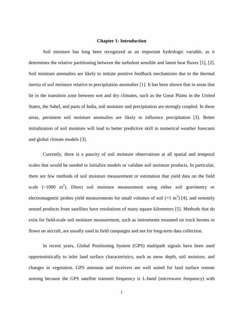
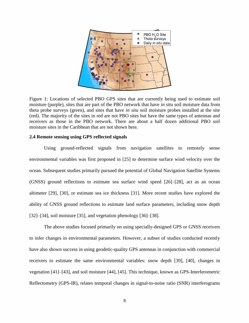
Figure 1: Locations of selected PBO GPS sites that are currently being used to estimate soil
moisture (purple), sites that are part of the PBO network that have in situ soil moisture data from
theta probe surveys (green), and sites that have in situ soil moisture probes installed at the site
(red). The majority of the sites in red are not PBO sites but have the same types of antennas and
receivers as those in the PBO network. There are about a half dozen additional PBO soil
moisture sites in the Caribbean that are not shown here.
2.4 Remote sensing using GPS reflected signals
Using ground-reflected signals from navigation satellites to remotely sense
environmental variables was first proposed in [25] to determine surface wind velocity over the
ocean. Subsequent studies primarily pursued the potential of Global Navigation Satellite Systems
(GNSS) ground reflections to estimate sea surface wind speed [26]–[28], act as an ocean
altimeter [29], [30], or estimate sea ice thickness [31]. More recent studies have explored the
ability of GNSS ground reflections to estimate land surface parameters, including snow depth
[32]–[34], soil moisture [35], and vegetation phenology [36]–[38].
The above studies focused primarily on using specially-designed GPS or GNSS receivers
to infer changes in environmental parameters. However, a subset of studies conducted recently
have also shown success in using geodetic-quality GPS antennas in conjunction with commercial
receivers to estimate the same environmental variables: snow depth [39], [40], changes in
vegetation [41]–[43], and soil moisture [44], [45]. This technique, known as GPS-Interferometric
Reflectometry (GPS-IR), relates temporal changes in signal-to-noise ratio (SNR) interferograms

9
to changes in environmental parameters surrounding a GPS antenna for an area which scales
with the monument height [46].
2.5 GPS-Interferometric Reflectometry
The constellation of GPS transmitting satellites (up to 32 in number) sends out earth-
bound signals indiscriminately, with receiving antennas passively intercepting incoming signals.
Part of the incoming signal will travel directly from the GPS satellite to the receiving antenna
(called the direct signal), and part of the signal will reflect off of the ground of nearby surfaces
before being intercepted by the antenna (indirect, ground-reflected, or multipath signal).
The ground-reflected signal represents a source of noise that geodesists attempt to
suppress. Figure 2a shows that the indirect, or multipath, signal tends to pierce the antenna at low
angles—this is why the choke-rings are in place, to suppress this signal to the greatest extent
possible. The gain pattern of the antenna is also designed such that the antenna itself tries to
suppress information coming in from these angles. This causes the indirect signal to be small in
magnitude compared to the direct signal, the pierce-point of which is at higher elevation angles.
Figure 2: a. Geometry of a multipath signal, for antenna height (Ho) and satellite elevation angle
(E). Bold black lines represent the direct signal transmitted from the satellite. The gray line is the
reflected signal from the ground. The antenna’s phase center is shown as the small dot. The blue
line/outer ring (higher gain) represents the RHCP gain of the antenna. The red line/inner ring
(lower gain) represents the LHCP gain of the antenna. At 0˚, the RHCP and LHCP gains are
approximately -38 dB and -50 dB, respectively. At 90˚, the RHCP and LHCP gains are

10
approximately -20 dB and -40 dB, respectively. b. Photo of a GPS antenna located in an alfalfa
field near Boulder, Colorado.
GPS receivers record information about the amount of noise in the environment in signal-
to-noise ratio (SNR) interferograms. These data are satellite track specific, such that each track
on a given day has its own SNR data time series. SNR data are recorded as a function of time,
which is also a function of the elevation angle of the satellite with respect to the horizon (90
degrees defined as zenith). A GPS satellite will rise above the horizon, sending out signals,
eventually will pass overheard or nearly so (with respect to the antenna) and then eventually set.
Most satellites rise and set over different azimuths with respect to the antenna (Figure 3a). Here,
SNR data resulting from different satellite tracks will be referred to by the pseudo-random
number sequence (PRN) of the satellite as well as the quadrant that the ground-reflections come
from. Thus, if PRN 7 is rising in quadrant 4, the SNR data resulting from this pass will be
labeled as PRN 7 Q 4.
Figure 3: Plan view diagrams for the GPS station OKL3. The GPS antenna is in the situated at
the center of each diagram. (a) Reflection point diagram, which shows path traces for selected
satellites. Gaps in traces indicate problems with data from trees or other obstructions. Concentric
circles show distances illuminated by the first Fresnel zone at that elevation angle. (b) Fresnel
zones for selected satellite tracks, which show the total area illuminated by the first Fresnel zone
for each track at 5 degrees (large ellipse). (c) Digital elevation model for the GPS site.

11
At low satellite elevation angles, both the direct and indirect signals are greatly
suppressed, so the SNR is relatively low (Figure 4a). At these angles, the indirect signal
interferes with the direct signal. The frequency of the oscillating interference pattern is primarily
a function of the difference in path lengths. As the satellite rises overhead, the relative proportion
of the direct signal received increases due to the antenna’s gain pattern, which increases the SNR
and decreases the effect of the oscillation pattern (Figure 4a). The time that it takes for a satellite
to go from 5-30 degrees above the horizon is approximately one hour. Note that rarely is there
SNR data for a satellite below 5 degrees, as the receiver is often hardwired to not accept data
from such low angles.
Figure 4: (a) SNR interferogram from PRN 7, quadrant 4. Data are for DOY 120 in 2012 at the
Oklahoma GPS station (OKL3). (b) Same SNR data as in (a), but converted to a linear scale and

12
detrended with a low-order polynomial. (c) Detrended SNR interferograms from four different
satellite tracks for DOY 120 in 2012 at the Oklahoma GPS station (OKL3). Interferograms are
vertically offset for clarity. (d) Lomb-Scargle Periodograms for the interferograms in (c).
2.6 Signal-to-Noise Ratio Data
2.6.1 SNR Equation and metrics
The interference between the direct and reflected GPS signals is recorded in SNR
interferograms. For a typical geodetic-quality GPS antenna’s gain pattern, this interference is
greatest at satellite elevation angles smaller than 30 degrees, as shown in Figure 4a.
The influence of the direct signal is seen in a large arcing trend in the SNR interferogram
in Figure 4a. In order to remove this influence and only see the interference pattern, the SNR
interferogram is converted to a linear scale (volt/volt) (1) and then detrended with a low-order
polynomial, estimated for each satellite track on each day (Figure 4b).
𝑆𝑁𝑅𝑉/𝑉 = 10𝑆𝑁𝑅𝑑𝐵−𝐻𝑧 20⁄ (1)
Where: 𝑆𝑁𝑅𝑑𝐵−𝐻𝑧 are the raw data, and 𝑆𝑁𝑅𝑉/𝑉 are the data transformed to a linear, volt/volt,
scale. Hereafter, the V/V subscript is dropped for clarity.
The resulting, detrended data are shown in Figure 4b. Note that the interferogram itself is
quite noisy. This noise comes from irregularities in the environment and instrument noise. Each
satellite track will have its own interferogram for each day, examples of which are shown in
Figure 4c. The amplitude of the interferogram is partly determined by the transmit power of the
satellite. Newer satellites have higher transmit powers and thus higher amplitudes, relative to
interferograms for older satellites. Other factors that affect interferograms that are not the result
of changes in the environment include the length of the cable between the antenna and the
receiver and the internal temperature of the receiver.

13
The amplitude of the interferogram decreases as elevation angle increases—this is
primarily due to the gain pattern of the antenna. However, changes in soil moisture and
vegetation surrounding the antenna will also lead to elevation-angle dependent amplitude
changes, as will be shown in later chapters.
Detrended SNR data have previously been modeled using the following equation [47]:
𝑆𝑁𝑅 = 𝐴 cos (4𝜋𝐻0
𝜆sin 𝐸 + 𝜙) (2)
Where: H0 is the height of the antenna, E is the elevation angle of the satellite, A is a constant
amplitude, λ is the GPS wavelength, and ϕ is a phase shift. This expression assumes that the SNR
data have a constant frequency (4𝜋𝐻0
𝜆). The observations in Figure 4c show that A is not constant
but depends upon elevation angle. A and ϕ are found from the SNR data using least-squares
estimation, with H0 set to the best approximation of the height of the antenna.
Eq. (2) forms the foundation for remote sensing of soil moisture using GPS-IR. The
parameters in (2), A and ϕ, are two of four metrics that have been investigated with regards to
their utility in inferring changes in surface soil moisture. The simplification of A and ϕ being
independent of elevation angle, when at least A certainly is not independent, do make certain
aspects of soil moisture estimation not straightforward, as will be shown later. However, because
complications from topography, tilted surfaces, and slight differences in antenna gain patterns
exist in real data, it will be shown that implementing a more complicated parameterization of A
with elevation angle would not be practical.
Although A and ϕ are calculated under the assumption that H0 is a known constant, for
observed data, H0 must be derived empirically and varies between satellite tracks due to changes

14
in the microtopography surrounding an antenna. H0, or the ‘a priori reflector height’ is estimated
using a Lomb-Scargle Periodogram (LSP), which is a method of spectral analysis that is akin to a
Fourier transform, except that it can process the unevenly-sampled SNR data recorded by the
GPS receiver. The LSP returns the spectral amplitude of a range of frequencies in the
interferogram, and the dominant/peak frequency is converted to an effective reflector height, Heff,
using the following relationship [48]:
meff fH2
1 (3)
Where fm is the peak frequency of the LSP. The power of the dominant frequency will be
referred to as ALSP. In cases where Heff and H0 are identical or nearly so, ALSP and A will be equal
or nearly so. Examples of LSPs are shown in Figure 4d. Note that two of the satellite tracks from
Figure 4c do not have distinguishable, dominant frequencies relative to noise, as shown by the
LSPs in Figure 4d (orange and blue lines). Calculated phase and amplitude for these two tracks
will not be as reliable as phase and amplitude calculated from the other two satellite tracks,
shown in red and green.
In order to estimate H0, the median of a relatively long time series of Heff values are used.
What constitutes a long enough time series varies depending on the site conditions, though in
general the longer the time series, the better. However, one needs to ensure that the data are not
being chosen during times of year when there is likely to be snow or significant vegetation
present.
Together, A, ϕ, Heff, and ALSP constitute the four ‘SNR metrics’ that will be investigated
with regards to their sensitivities to changes in land surface characteristics.

15
2.6.2 Temporal changes in SNR metrics
Observed time series of the four SNR metrics each undergo data processing before they
may be compared to time series of SNR metrics from different satellite tracks. The absolute
magnitudes of both A and ALSP are primarily contolled by the transmit power of the particular
GPS satellite—newer satellites have higher transmit powers. The time series in Figure 5 show
time series for both A and ALSP from two satellite tracks. All of the time series exhibit similar
seasonal fluctuations throughout the year; however, both A and ALSP for PRN 5 are consistently
higher than for PRN 12, indicating a higher transmit power for PRN 5.
Figure 5: (left column) Raw SNR metric time series for four satellite tracks at the GPS station
OKL3. There is significant noise present in all four time series around 2011.1, indicating a snow
16
event. (right column) The corresponding zeroed, normalized, or differenced metric time series.
The snow signature has not been removed from these time series.
In order to compare relative changes in the A and ALSP time series across satellite tracks
and GPS sites, each time series is normalized with respect to the mean of the top 20% of the data
in each time series:
𝐴𝐿𝑆𝑃𝑛𝑜𝑟𝑚 = 𝐴𝐿𝑆𝑃 𝐴𝐿𝑆𝑃20% ⁄ (4)
𝐴𝑛𝑜𝑟𝑚 = 𝐴 𝐴20% ⁄ (5)
Where: 𝐴20% and 𝐴𝐿𝑆𝑃20%
are the mean of the top 20% of data from each time series. 𝐴𝑛𝑜𝑟𝑚 and
𝐴𝐿𝑆𝑃𝑛𝑜𝑟𝑚 are thus unitless measures of relative change in each satellite track’s amplitude time
series (see Figure 5 for examples of the conversion).
Similarly, the absolute magnitude of Heff varies between satellite tracks due to differences
in microtopography surrounding the antenna. In order to see relative changes in Heff, the Heff time
series is subtracted from the estimated antenna height, yielding ΔHeff:
∆𝐻𝑒𝑓𝑓 = 𝐻0 − 𝐻𝑒𝑓𝑓 (5)
Example time series of the conversion between Heff and ΔHeff are shown in Figure 5.
Phase, calculated under the assumption that antenna height is equal to H0, is also
characterized as having a satellite-track specific ‘baseline’ value, as shown in Figure 5. Figure 5
shows that each ϕ time series exhibits similar seasonal and higher frequency fluctuations, despite
the different baseline values. The baseline phase value for each satellite track is determined by
many factors, such as tilting of the ground surface and errors in H0 estimation. When the baseline
values are subtracted from each track’s time series, as in Figure 5, data are more easily

17
comparable to one another. For empirical data, the following equation is used to ‘zero’ each
phase time series.
∆𝜙 = ∆𝜙𝑜𝑏𝑠 − ��30% (10)
Where ��30% is the mean of the lowest 30% of observed phase values for a specific year.
Phase data tend to be zeroed on a per-year basis, whereas amplitude normalization and effective
reflector height differencing tend to use the entire time series. The reason for this will be
described in Chapter 6.2.
All further analyses will show results in terms of ∆𝜙, ∆𝐻𝑒𝑓𝑓, 𝐴𝑛𝑜𝑟𝑚, and 𝐴𝐿𝑆𝑃𝑛𝑜𝑟𝑚.

18
Chapter 3: Ground truth experiments and data
In order to investigate the sensitivity of GPS-IR to changes in soil moisture and
vegetation in field settings, dozens of vegetation surveys were conducted, and several years’
worth of in situ soil moisture data were collected, either using permanently-installed probes or
from surveys with a theta probe. This section summarizes the field data. The data were used for
validating the electrodynamic soil and vegetation model described in Chapter 4 as well as
validating soil moisture retrievals using GPS-IR described in Chapter 6.
3.1 Description of measurement techniques
3.1.1 In situ soil moisture data
3.1.1.1 Time domain reflectometry probes
Fig. 1 from Chapter 2.2 shows a map of GPS sites that either have permanently-installed
soil moisture probes (red points) or have at least one soil moisture survey (green points). The
majority of the sites with permanently-installed probes are not part of the PBO network, with the
exception of p041 in north-western Colorado, though most of these sites are part of the PBO H2O
network. Most stations have been providing 30-minute soil moisture data for approximately the
past five years. Time-domain reflectometry probes at these sites are Campbell Scientific 616
moisture probes. The typical installation at the GPS sites is as follows: 3 or more probes are
connected to a data logger powered near the GPS receiver. Each probe has at least a 40 ft. long
cable connecting the data logger to the probe itself, which means probes may be installed up to
40 feet away from the GPS antenna. The probes tend to be installed south of the antenna and at
least 10 or more feet away from one another, in order to record spatial heterogeneities in soil
moisture. The first 3-5 probes are buried at a depth of only 2.5 cm. This depth actually gives a

19
vertical-average of the soil moisture between 0-5 cm. If there are more probes available at the
site, they are buried at 7.5 cm, which gives the average soil moisture between 5-10 cm. At a few
sites, there are also probes buried at 20 cm, and in rare cases, 40 cm.
Time-domain reflectometry probes, like the CS 616s, emit an electromagnetic pulse that
travels down the length of the rod and is reflected back to its source. The velocity of the pulse
depends on the dielectric permittivity of the surrounding medium (in this case, soil). The higher
the moisture content of the soil, the higher the permittivity, and the slower the signal velocity
[49]. The probes record the time it takes between the emitted pulse and the subsequent received
reflection, and if the length of the probe is known, travel velocity may be calculated. The
velocity of the reflected signal is related to the moisture content, using the factory-calibrated
relationships. Factory calibrations may not be representative of true field conditions if the
conductivity of the soil is unusually high, if the soil is compacted, or if the soil has a high clay
content. In these situations, more accurate results would be achieved using a field-specific
calibration. We have used the factory calibration (quadratic fit) at all of our field sites since there
is a good correlation between our probe data and data from volumetric samples.
Variations in ground temperature are a significant source of error in soil moisture
estimations using the CS616 probes that we account for at all of the sites. A standard temperature
correction is used before conversion to soil moisture, using Cambpell Scientific temperature
probes (thermistors) buried at either 2.5 cm or 7.5 cm depth. In cases where there are probes
buried at 20 or 40 cm, these data are not corrected for temperature effects.

20
3.1.1.2 Theta probe surveys
We have conducted several theta probe surveys at select GPS sites, which yield estimates
of soil moisture content over the top 6 cm of the soil column. Many of these sites are PBO
stations, and some sites have data from both CS616 and theta probe surveys. The theta probe we
use is the ML3, manufactured by Delta-T Devices. The theta probe also emits an electromagnetic
pulse into the soil and measures the resulting voltage, relating the voltage to the refractive index
of the soil, which is close to the square root of the permittivity [50]. The ML3 probe provides
factory calibrations to relate the recorded voltage to the moisture content of mineral and organic
soils. We use the factory calibration for the organic soil to produce our soil moisture estimates.
These data are not corrected for temperature.
Theta probe surveys consist of several point measurements within 35 m of a GPS
antenna, usually on the order of 20-30 measurements, which are then averaged.
3.1.1.3 Gravimetric soil moisture surveys
Gravimetric soil moisture surveys have also been conducted at selected GPS stations.
Gravimetric soil moisture sampling is one of the only ways to directly measure soil moisture.
Gravimetric sampling involves inserting a column (usually metal) with a known volume
vertically into the soil and removing all of the soil contained within the column. The soil is
weighed, dried at 100 degrees Celsius for 24 hours, and then weighed again. This method may
provide a measurement of volumetric moisture content, assuming the density of water is 1000 kg
m-3
.

21
3.1.2 Vegetation surveys
At GPS sites with vegetation field data, vegetation samples are generally collected
regularly throughout the growing season, though some sites only have a few surveys. An
individual vegetation sampling survey consists of collecting seven vegetation samples, at random
azimuths and distances (between 7-35 m), around an antenna. At each sampling location, a 30 x
30 cm or 50 x 50 cm grid is tossed on the ground, and vegetation canopy height is measured. The
measured canopy height is meant to represent the 90th
percentile height. For some very
heterogeneous environments, the height measurement may not be representative of the
vegetation that is actually within the sampling grid. All of the vegetation within the grid is then
cut and weighed. The cut vegetation is then dried for 48 hours at 50 degrees Celsius and weighed
again, to measure how much water was in each sample. The dried vegetation is referred to as the
dry biomass. Once the data from the seven samples are averaged, we have estimates of the mean
canopy height, water content, and dry biomass on each day that samples were collected. This
vegetation collection does not modify site characteristics to any noticeable degree, given the
relatively larger sensing area of each antenna. For example, 15 sampling days during a growing
season would disturb only 10 m2 of vegetation, about 1% of the sensing area within the GPS
footprint.
3.2 Data Summary
3.2.1 Soil Moisture Data
Figure 6 shows the distributions of 30-minute soil moisture using data from the CS616
probes for each GPS station that has data. Data are grouped by rough site location; for example
the three wheat/oat sites are labeled “Wheat,” and the sites in Oklahoma are labeled

22
“Rangeland.” Note that most of the soil moisture distributions are not Gaussian, which means
using statistics like the mean or median will be slightly misleading.
Figure 6: Distributions of 30-minute soil moisture content for the GPS stations with CS 616
probes. Data are from probes buried at 2.5 cm depth.
Table 2 indicates how many theta probe and gravimetric soil moisture surveys exist at
official and provisional PBO H2O sites. More surveys have been conducted at other sites that are
not sites used for soil moisture estimation.
Table 2: Summary of theta probe and volumetric soil moisture surveys conducted at GPS
stations. The horizontal line indicates that split between our validation sites and PBO sites.
Site Years Total # of theta
survey points
Total # of gravimetric
survey points
OKL2 2011-2012 33 0
OKL3 2011-2012 33 0

23
OKL4 2011-2012 32 0
P041 2014 25 4
bcgr 2011-2014 38 15
Oats 2012 14 3
ames 2012 1 2
Bcw2 2011 5 8
P036 2013-2014 5 1
P070 2013-2014 5 1
P040 2013-2014 5 1
P037 2013-2014 5 1
P039 2013-2014 5 1
P123 2014 3 0
P035 2014 2 0
P038 2014 2 0
P032 2013 2 2
P042 2013 2 2
P360 2013 1 1
P048 2011 0 1
P049 2011 0 1
P050 2011 0 1
P053 2011 0 1
P103 2011 0 1
P678 2011 0 1
P679 2011 0 1
P684 2011 0 1
24
P719 2011 0 1
P722 2011 0 1
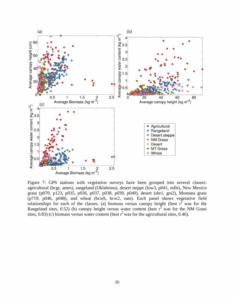
3.2.2 Vegetation Data
Table 3: GPS stations, antenna heights, and vegetation information shows, for many of
the stations for which we have vegetation field data, the range of wet weight (Mf), dry biomass
(Md), and canopy height (Hveg) measurements. The sites vary significantly from one another,
depending on the vegetation type. For example, the vegetation at the alfalfa site can contain more
than three times the amount of water as the vegetation at the rangeland sites. Figure 7 shows
vegetation data from field surveys in the form of how different vegetation parameters vary with
one another. In this figure, GPS stations have been grouped into different classes, which depend
on either the location of the GPS antenna or the vegetation type. Each point in Figure 7 is the
average of each vegetation field survey. Figure 7a shows how vegetation biomass and canopy
height vary with one another, depending on the vegetation group. Plotting biomass on the x-axis
is not meant to imply that biomass determines canopy height. The outliers in the agricultural
group (red points) are bcgr 2013 (alfalfa field) data, which differ from the other data due to
heavy rains that caused the canopy to fall over and made measurement difficult. There tends to
be a good relationship between biomass and canopy height within vegetation groups. Figure 7b
shows the relationship between canopy height and water content. There is more scatter in this
relationship than between biomass and height, especially for the agricultural sites. Figure 7c
shows the relationship between canopy biomass and water content. There is a good relationship
between 2010-2012 agricultural data, but no clear relationships for the other vegetation groups.

25
The relevance of Figure 7 will be described in Chapter 4.4. For now, the important thing
to keep in mind is that there is a large amount of variability in the relationships between
vegetation parameters, even within the same vegetation class. These relationships change
throughout a growing season and between growing seasons. General conclusions about the
vegetation characteristics at a site could be made based on class (i.e. “At grasslands, it is unlikely
the water content will exceed 1 kg m-2
”), but conclusions with any more detail would be difficult
to draw.
Table 3: GPS stations, antenna heights, and vegetation information
26
Figure 7: GPS stations with vegetation surveys have been grouped into several classes:
agricultural (bcgr, ames), rangeland (Oklahoma), desert steppe (low3, p041, mfle), New Mexico
grass (p070, p123, p035, p036, p037, p038, p039, p040), desert (shr1, grs2), Montana grass
(p719, p046, p048), and wheat (bcwh, bcw2, oats). Each panel shows vegetative field
relationships for each of the classes. (a) biomass versus canopy height (best r2 was for the
Rangeland sites, 0.52) (b) canopy height versus water content (best r2 was for the NM Grass
sites, 0.83) (c) biomass versus water content (best r2
was for the agricultural sites, 0.46).
27
Chapter 4: Forward modeling of SNR data in relation to soil moisture and vegetation
In this chapter, I describe an electrodynamic model that simulates how SNR
interferograms (and their resulting metrics) are affected by changing the moisture content of the
soil as well as changing vegetation canopy parameters. Data from the previous chapter will be
used to validate this model. Modeling interferograms is useful because observed SNR metric
time series from different satellite tracks, even at the same site, show large differences, as in
Figure 5. There are many complicating factors that exist in observed data that cannot always be
adequately quantified or identified (temperature effects, spatial heterogeneities, azimuthal
differences in gain pattern, etc.). Modeling is the only way to remove these effects and only look
at contributions of soil moisture and vegetation parameters to changes in SNR data.
This chapter is organized as follows. First, the model architecture is described. I cannot
take credit for the majority of the model development; the heavy lifting in model design was all
accomplished by Valery Zavorotny of NOAA. However, in order to better understand the
contribution that I made to the model (addition of a vegetation canopy), it is necessary to
describe the model from the ground up. The model is then validated, using observed SNR data,
vegetation field data, and in situ soil moisture data for comparison. Next, how soil moisture
content affects SNR metrics for a bare soil is quantified. A simple relationship is derived for
estimating soil moisture using SNR metrics. Following this, the effect of adding a vegetation
canopy on SNR metrics is explored, assuming that the moisture content of the soil does not
change. The most important canopy parameters are identified, and the influence of interactions
between parameters on metrics is explored. Finally, the effect of changing the underlying soil
moisture content, with variable overlying vegetation, on SNR metrics is investigated.

28
4.1 Model architecture
The theoretical basis for the relationships between SNR metrics and soil and vegetation
parameters is derived from a 1-D, electrodynamic, single-scattering, forward model. The
foundation for the model was developed in [51]. The model simulates SNR interferograms, from
which metrics may be calculated, given antenna, soil, and vegetation canopy information as input
parameters. The model assumes that the topography surrounding the antenna is perfectly smooth,
though some experiments with adding surface roughness have been done. A large part of this
project was adapting the model foundation, which was developed for bare soil simulations, to
include the effects of a vegetation canopy.
4.1.1 Reflection coefficient calculations
The core component of the model is the numerical calculation of reflection coefficients
for a GPS signal reflecting from a surface. The procedure for calculating the coefficients is
presented in [10]. For a vertically layered medium with arbitrary dielectric constants assigned to
each layer, the model calculates the horizontal and vertical polarization reflection coefficients for
the signal reflecting out of each layer, taking into consideration absorption within each layer. The
soil layers in the model are very thin—fractions of a millimeter, so the model is basically
calculating reflection coefficients for a continuous profile. Calculation of coefficients is outlined
in the following equations:
𝜀𝑚 = 𝜀𝑚′ + 𝑖𝜀𝑚
′′ (3)
𝑅𝐻𝑡 = √𝜀𝑚+1−𝜀𝑀𝑠𝑖𝑛2𝜃−√𝜀𝑚−𝜀𝑀 𝑠𝑖𝑛2 𝜃
√𝜀𝑚+1−𝜀𝑀𝑠𝑖𝑛2𝜃+√𝜀𝑚−𝜀𝑀 𝑠𝑖𝑛2 𝜃 (4)
𝑅𝑉𝑡 = 𝜀𝑚√𝜀𝑚+1−𝜀𝑀𝑠𝑖𝑛2𝜃−𝜀𝑚+1√𝜀𝑚−𝜀𝑀 𝑠𝑖𝑛2 𝜃
𝜀𝑚√𝜀𝑚+1−𝜀𝑀𝑠𝑖𝑛2𝜃+𝜀𝑚+1√𝜀𝑚−𝜀𝑀 𝑠𝑖𝑛2 𝜃 (5)
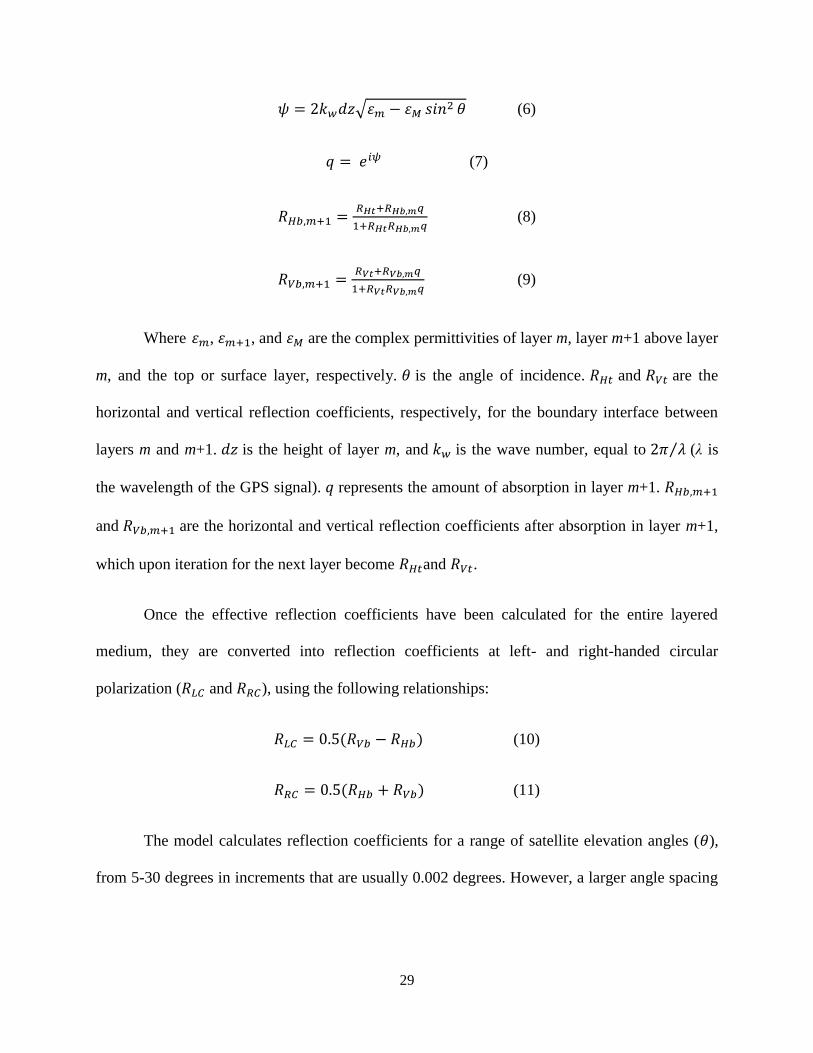
29
𝜓 = 2𝑘𝑤𝑑𝑧√𝜀𝑚 − 𝜀𝑀 𝑠𝑖𝑛2 𝜃 (6)
𝑞 = 𝑒𝑖𝜓 (7)
𝑅𝐻𝑏,𝑚+1 =𝑅𝐻𝑡+𝑅𝐻𝑏,𝑚𝑞
1+𝑅𝐻𝑡𝑅𝐻𝑏,𝑚𝑞 (8)
𝑅𝑉𝑏,𝑚+1 =𝑅𝑉𝑡+𝑅𝑉𝑏,𝑚𝑞
1+𝑅𝑉𝑡𝑅𝑉𝑏,𝑚𝑞 (9)
Where 𝜀𝑚, 𝜀𝑚+1, and 𝜀𝑀 are the complex permittivities of layer m, layer m+1 above layer
m, and the top or surface layer, respectively. 𝜃 is the angle of incidence. 𝑅𝐻𝑡 and 𝑅𝑉𝑡 are the
horizontal and vertical reflection coefficients, respectively, for the boundary interface between
layers m and m+1. 𝑑𝑧 is the height of layer m, and 𝑘𝑤 is the wave number, equal to 2𝜋 𝜆⁄ (λ is
the wavelength of the GPS signal). 𝑞 represents the amount of absorption in layer m+1. 𝑅𝐻𝑏,𝑚+1
and 𝑅𝑉𝑏,𝑚+1 are the horizontal and vertical reflection coefficients after absorption in layer m+1,
which upon iteration for the next layer become 𝑅𝐻𝑡and 𝑅𝑉𝑡.
Once the effective reflection coefficients have been calculated for the entire layered
medium, they are converted into reflection coefficients at left- and right-handed circular
polarization (𝑅𝐿𝐶 and 𝑅𝑅𝐶), using the following relationships:
𝑅𝐿𝐶 = 0.5(𝑅𝑉𝑏 − 𝑅𝐻𝑏) (10)
𝑅𝑅𝐶 = 0.5(𝑅𝐻𝑏 + 𝑅𝑉𝑏) (11)
The model calculates reflection coefficients for a range of satellite elevation angles (𝜃),
from 5-30 degrees in increments that are usually 0.002 degrees. However, a larger angle spacing

30
does not significantly affect conclusions for how resulting SNR interferograms vary with
environmental input parameters.
4.1.2 Permittivity profile generation: Soil
For GPS-IR, the layered medium of interest is a soil with an overlying vegetation canopy.
As stated previously, the permittivity of a soil at microwave frequencies is predominantly
dependent on its moisture content, though there is a second-order dependence on soil texture, or
the relative amounts of sand, silt, and clay within the soil. The relationships between soil texture,
moisture content, and permittivity at microwave frequencies is fairly well studied. This model
uses relationships found in [9], [52] which presents complex permittivity measurements using
semi-empirical relationships for 1.4 GHz (L-band), five soil textures ranging from a sandy loam
to a silty clay, and a wide range of moisture contents.
The soil component of the model requires user-specified volumetric soil moisture
estimates at variable depths in the soil column and as well as a soil texture. The depths at which
soil moisture is specified is up to the user, though the model does not currently consider moisture
contents below 20 cm depth. Specified moisture contents are allowed to vary between 0.01 and
0.5 cm3 cm
-3. The model discretizes, interpolates, and extrapolates as necessary the input
moisture contents using a cubic spline to create a vertical soil moisture profile with soil layers
that are generally 0.1 mm thick, though this parameter may be specified. The vertical soil
moisture profile is then converted to a vertical complex permittivity profile, using the specified
soil texture and semi-empirical relationships found in [9] in a lookup table.

31
4.1.3 Permittivity profile generation: Vegetation
A vertical permittivity profile of the overlying vegetation canopy, if there is one present,
must also be calculated. Although the model is able to accommodate the addition of vegetation
layers (analogous to the soil layers), here I assume the vegetation canopy is comprised of only
one layer, the reason for which is discussed below. The permittivity of vegetation material has
been the subject of many studies [53]–[56]; however, empirical measurements are more difficult
to make than for soil, and other properties than water content (i.e. volume fraction of vegetation
within the canopy) affect the overall permittivity of the vegetation canopy. A lookup table of
permittivity estimates is not possible here. Most empirical measurements of vegetation
permittivity focus on vegetation that is already mostly dried, so there are not many published
data on the range of permittivities possible for a specific vegetation type. In addition, the
permittivity of the vegetation material itself will be quite different from the effective permittivity
of the canopy, which itself is a mixture of vegetation material and air. Few studies exist that
directly attempt to measure the permittivity of a vegetation canopy, and those that do note that
the volume fraction of vegetation within the canopy is an important factor [56]. The volume
fraction of vegetation within the canopy will be highly dependent on vegetation type and will
vary depending on the point in the growth cycle.
Due to the complexities described above, it is most common to use a model to estimate
vegetation permittivity. The vegetation permittivity model that is used here was developed in
[55]. This model was validated using data from corn leaves and only calculates the permittivity
of the vegetation material, not of a canopy, which would include contributions from both
vegetation and air. It requires user-specified input parameters of signal frequency, vegetation
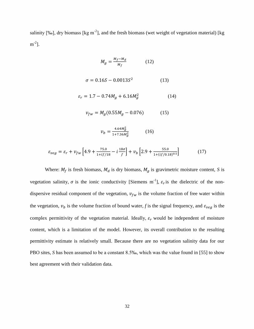
32
salinity [‰], dry biomass [kg m-2
], and the fresh biomass (wet weight of vegetation material) [kg
m-2
].
𝑀𝑔 =𝑀𝑓−𝑀𝑑
𝑀𝑓 (12)
𝜎 = 0.16𝑆 − 0.0013𝑆2 (13)
𝜀𝑟 = 1.7 − 0.74𝑀𝑔 + 6.16𝑀𝑔2 (14)
𝑣𝑓𝑤 = 𝑀𝑔(0.55𝑀𝑔 − 0.076) (15)
𝑣𝑏 =4.64𝑀𝑔
2
1+7.36𝑀𝑔2 (16)
𝜀𝑣𝑒𝑔 = 𝜀𝑟 + 𝑣𝑓𝑤 [4.9 +75.0
1+𝑖𝑓/18− 𝑖
18𝜎
𝑓] + 𝑣𝑏 [2.9 +
55.0
1+(𝑖𝑓/0.18)0.5] (17)
Where: 𝑀𝑓 is fresh biomass, 𝑀𝑑 is dry biomass, 𝑀𝑔 is gravimetric moisture content, S is
vegetation salinity, 𝜎 is the ionic conductivity [Siemens m-1
], 𝜀𝑟 is the dielectric of the non-
dispersive residual component of the vegetation, 𝑣𝑓𝑤 is the volume fraction of free water within
the vegetation, 𝑣𝑏 is the volume fraction of bound water, f is the signal frequency, and 𝜀𝑣𝑒𝑔 is the
complex permittivity of the vegetation material. Ideally, 𝜀𝑟 would be independent of moisture
content, which is a limitation of the model. However, its overall contribution to the resulting
permittivity estimate is relatively small. Because there are no vegetation salinity data for our
PBO sites, S has been assumed to be a constant 8.5‰, which was the value found in [55] to show
best agreement with their validation data.

33
Once the permittivity of vegetation material has been determined, the permittivity of the
canopy is calculated. The model assumes that the only constituents in the canopy are vegetation
and air, or:
𝑣𝑡𝑜𝑡𝑎𝑙 = 𝑣𝑎𝑖𝑟 + 𝑣𝑣𝑒𝑔 (18)
The volume fraction of vegetation within the canopy, 𝑣𝑣𝑒𝑔, is determined to be:
𝑣𝑣𝑒𝑔 = 𝑀𝑓
𝐻𝑣𝑒𝑔×𝜌𝑣𝑒𝑔 (19)
Where: Hveg is the height of the canopy, and 𝜌𝑣𝑒𝑔 is the true density of vegetation
material [kg m-3
]. Eq. 19 simply calculates how ‘spread-out’ the water and bulk vegetation
material is in the canopy. 𝜌𝑣𝑒𝑔 is expected to vary with vegetation type and moisture content, and
its relationship with moisture content can be somewhat unintuitive. For example, if one assumed
that the volume of vegetation material stays the same regardless of moisture content, the addition
of water would increase 𝜌𝑣𝑒𝑔 to a maximum value of 1000 kg m-3
, if gravimetric moisture
content were 100%. However, in reality it can be assumed that when vegetation water content
decreases, the volume will shrink an amount proportional to that of the lost water [55] and vice
versa. The exact relationship will depend on plant type and even within specific plant geometric
components. For example, the dependence of true density with moisture content of plant seeds
has been shown to be a parabolic function of moisture content for some seed types [57].
Unfortunately, there is a dearth of published data for a wide range of moisture content and
natural plant types (most studies address fruits and seeds). 𝜌𝑣𝑒𝑔 is an important parameter for
determining effective canopy permittivity. In model validation, discussed in a later section, we
assumed 𝜌𝑣𝑒𝑔 to be directly proportional to water content, which assumes volume changes to be
34
negligible, and found good agreement with observations. In the vegetation filter, which is also
discussed in a later section, we no longer assume this relationship to ensure the filter can be
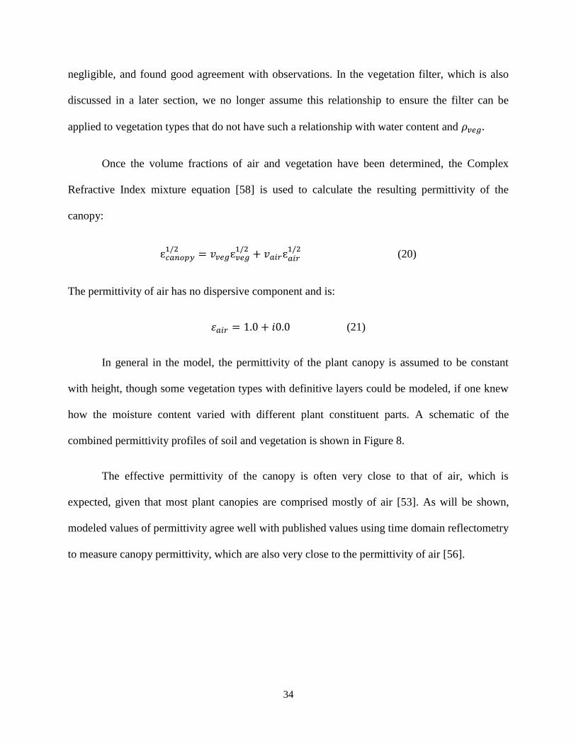
applied to vegetation types that do not have such a relationship with water content and 𝜌𝑣𝑒𝑔.
Once the volume fractions of air and vegetation have been determined, the Complex
Refractive Index mixture equation [58] is used to calculate the resulting permittivity of the
canopy:
ɛ𝑐𝑎𝑛𝑜𝑝𝑦1/2
= 𝑣𝑣𝑒𝑔ɛ𝑣𝑒𝑔1/2
+ 𝑣𝑎𝑖𝑟ɛ𝑎𝑖𝑟1/2
(20)
The permittivity of air has no dispersive component and is:
𝜀𝑎𝑖𝑟 = 1.0 + 𝑖0.0 (21)
In general in the model, the permittivity of the plant canopy is assumed to be constant
with height, though some vegetation types with definitive layers could be modeled, if one knew
how the moisture content varied with different plant constituent parts. A schematic of the
combined permittivity profiles of soil and vegetation is shown in Figure 8.
The effective permittivity of the canopy is often very close to that of air, which is
expected, given that most plant canopies are comprised mostly of air [53]. As will be shown,
modeled values of permittivity agree well with published values using time domain reflectometry
to measure canopy permittivity, which are also very close to the permittivity of air [56].

35
Figure 8: Schematic of the combined soil moisture and vegetation permittivity profiles.
4.1.4 Note on the plane-stratified model for a vegetation canopy
The model I have presented here is a plane-stratified model—many studies have used
plane-stratified models to simulate emission from vegetation canopies at microwave frequencies
(e.g. [59], [60]). This is in contrast to a geometrical modeling approach, in which each
component of the plant canopy, such as stalks and leaves, is modeled by their geometrical shapes
(e.g. [15], [61]). Geometrical modeling is used because, at microwave frequencies, a canopy
layer is often considered inhomogeneous and anisotropic [54]. Geometric effects are most
important when the components of the canopy, i.e. stalks, leaves, or branches, are the same size
or larger than the wavelength of the signal. Because the wavelength of the GPS L-band signal is
~24 cm, which is much longer than X- or C-bands (~3 and 5 cm, respectively), we use a plane-
stratified model that does not consider internal canopy geometry. Geometric models, which
would take into account the relative distribution and orientation of stalks of leaves, are
commonly used in radar remote sensing and would likely lead to better agreement with
observations. We decided on a plane-stratified approach due to its ability to use only
commonly-measured field parameters as input, with no additional information needed about
individual plant components. For natural, non-forested environments, geometric components of

36
the canopy tend to be smaller than the wavelength of the L-band signal. The model might not
accurately simulate vegetation types that have geometric components of greater than 24 cm.
Assuming that structural geometric effects are negligible means that coherence losses of
the reflected wave due to volume scattering within the plant canopy due to geometric effects are
neglected. However, the model can take into account multiple reflections between one-
dimensional layers within the medium, if they are specified, which does allow for modeling the
resulting coherence loss from permittivity changes.
4.1.5 Calculation of direct and indirect power
The permittivity profiles for soil and the optional vegetation layer are used in the
reflection coefficient calculations, described in Section 4.1.1. After reflection coefficients are
calculated, they must be combined with the antenna gain pattern to calculate direct and indirect
power, from which an SNR interferogram may be simulated. A more detailed explanation of this
part of the model is found in [51]. Complex signal amplitudes, both reflected (ref) and direct
(dir) for both circular polarization components (R for right-handed and L for left-handed) are
calculated. Because the direct signal is only right-handed circularly polarized, the left-handed
component of this term is zero. The gain pattern, G, is specified by the user for both right- and
left-handed polarizations, at all elevations (assumed to be azimuthally symmetrical). The gain
pattern used in the model is for a choke ring antenna, whose radiation pattern was measured in an
anechoic chamber.
An additional phase shift term (unrelated to ϕ calculated from the SNR interferogram)
must be included in the reflected powers to account for the extra path delay from the direct and
reflected signal. This geometric phase delay is a function of the a priori reflector height, H0.

37
When there is significant vegetation or snow present, the height of either the vegetation canopy
or snow layer has to be subtracted first. Equations for complex signal amplitudes and geometric
phase shifts are summarized below.
Φ = 2𝑘𝑤𝐻0 cos 𝜃 (22)
𝑢𝑅𝑑𝑖𝑟 = 𝐺𝑅𝑑𝑖𝑟 (23) 𝑢𝑅𝑟𝑒𝑓 = 𝐺𝑅𝑟𝑒𝑓 × 𝑅𝑅𝐶 × 𝑒𝑖𝜋Φ (24)
𝑢𝐿𝑑𝑖𝑟 = 0 (25) 𝑢𝐿𝑟𝑒𝑓 = 𝐺𝐿𝑟𝑒𝑓 × 𝑅𝐿𝐶 × 𝑒𝑖𝜋Φ (26)
𝑢𝑅 = 𝑢𝑅𝑟𝑒𝑓 + 𝑢𝑅𝑑𝑖𝑟 (27) 𝑢𝐿 = 𝑢𝐿𝑟𝑒𝑓 + 𝑢𝐿𝑑𝑖𝑟 (28)
𝑢𝑑𝑖𝑟 = 𝑢𝐿𝑑𝑖𝑟 + 𝑢𝑅𝑑𝑖𝑟 (29) 𝑢𝑟𝑒𝑓 = 𝑢𝐿𝑟𝑒𝑓 + 𝑢𝑅𝑟𝑒𝑓 (30)
The incoherent power received is:
𝑃𝐼 = |𝑢𝑢𝑝|2
+ |𝑢𝑑𝑛|2 (31)
The coherent power received is:
𝑃𝐶 = |𝑢𝑅 + 𝑢𝐿|2 (32)
Although observed SNR interferograms must be detrended with a low-order polynomial
to remove the effect of the direct signal, because both coherent and incoherent power are known
in the model, the incoherent power can simply be subtracted from the coherent power to produce
the detrended interferogram. The interferogram is multiplied by 105
in order for the amplitude to
be the correct magnitude.
𝑆𝑁𝑅 = 𝑃𝐶 − 𝑃𝐼 (33)

38
4.2 Model validation
In this section, the soil and vegetation model is validated using SNR observations and in
situ measurements of soil moisture and vegetation field data. The purpose of model validation is
to evaluate whether the model can successfully simulate SNR data observed in the field. First,
the modeled and observed SNR curves are compared, calculating how the correlation between
modeled and observed data varies with vegetation water content. Here, we test the assumption
that the vegetation canopy can be characterized as one bulk layer by also testing a gradually-
varying canopy top. Then, whether or not the model can reproduce observed SNR metrics and
how they vary with vegetation parameters is evaluated.
4.2.1 Validation Set-Up: Field Observations and Model Input
The validation data comprise observed SNR data from GPS antennas located in different
vegetative environments. Antennas are surrounded by a managed alfalfa field (BCGR), a
cultivated soybean field (AMES), a grazed rangeland (OKL2, OKL3, OKL4), and a desert steppe
(p041). The GPS systems at these sites have identical hardware (Trimble NetRS receivers and
Choke-Ring antennas with a radome), though the height of each antenna varies slightly. Some of
the field sites have multiple antennas operating concurrently and/or located closely to one
another; this information is summarized in Table 3.
Each of the sites is also instrumented with Campbell Scientific 616 soil moisture probes
(at least five probes at 2.5 cm depth, five at 7.5 cm, and two at 20 cm). The soil moisture probes
each record data every 30 minutes, though here the data are averaged from the probes to get one
daily value at each depth. Vegetation samples were collected regularly throughout the growing
season (see Table 3 for vegetation statistics). The samples were collected using the procedure as
described in Chapter 3. Data from vegetation samples collected during each survey were
39
averaged, such that we have estimates of the mean canopy height, water content, and dry
biomass on each day that samples were collected.
The vegetation field observations and soil moisture observations for each day are
averaged and are used as the inputs to the soil-vegetation model. Thus, each sampling day has
one corresponding modeled SNR curve generated using the mean vegetation and soil moisture
data collected on that day.
Because observed SNR data from different satellite tracks are characteristically different,
I compare the model simulations to observations from several satellite tracks. Observed SNR
data from five satellite tracks are used for most sites, though only two and three tracks from
Antennas D and E at the rangeland site are used, respectively. Tracks were selected such that
none were influenced by trees or had significant topography (much greater than 5%). Phase,
amplitude, and effective reflector height are computed from the SNR data from each satellite
track. H0 for each satellite track was determined empirically. Amplitude was normalized for each
site by dividing each daily-mean amplitude value by the maximum daily-mean amplitude
observed at that site. Because the height of the GPS antenna is different for every site, we only
looked at Heff deviations from H0 (ΔHeff).
Phase was zeroed with respect to the median phase value. For the four field sites, this
occurs during times of the year when vegetation is either dormant or absent. We also zero our
modeled phase values, though a slightly different approach had to be used. There are relatively
few modeled phase values in our time series because the model is only run for days when
vegetation was sampled. Therefore, we chose the zeroing value to be the value that corresponds
to the lowest observed vegetation wet weight. After zeroing observed and modeled phase time

40
series, both are approximately zero when there is little to no vegetation and are less than zero
when vegetation grows.
4.2.2 Comparison of Simulated and Observed SNR Data
The first goal of model validation is to evaluate whether modeled SNR data matches well
with observed. Comparing SNR data requires that one curve is shifted to account for offsets
introduced by the different baseline phase values of different satellite tracks. Because of this, we
performed a cross-correlation on the modeled and observed SNR curves to determine the phase
lag that would allow for the highest correlation (𝛾) between the two curves. This shifting is done
on a track-by-track basis. The modeled data are thus shifted to best match the observed data. This
means that when we compare the shapes of modeled and observed SNR data, we are comparing
their shape only and not how their respective phases change due to soil moisture or vegetation.
The modeled and observed phase shifts are compared separately.
Two examples of observed and modeled SNR data from the soybean site are shown in
Figure 9a,b. The observed SNR data are from one satellite track—different satellite tracks have
slightly different SNR data. The modeled SNR curves for bare soil and vegetated conditions
match the corresponding observed SNR curves. The model reproduces the reduction of
amplitude resulting from the addition of vegetation. In addition, variations in amplitude with
elevation angle that result from the presence of vegetation are also well simulated. The SNR data
simulated using the gradual canopy top (meaning the permittivity was allowed to decrease to 1.0
over the top 10% of the canopy) does not match observations as well as the SNR data simulated
with the homogeneous canopy, although the differences between the two are small compared to
the changes associated with adding a vegetation canopy.

41
Figure 9: (a) Black line is SNR data from one satellite passing over the soybean site when
ground was bare. Blue line is one modeled representation with a soil moisture of 0.15 cm3 cm
-3,
using field inputs from the same day as the observed data. (b) Same as in a., except for when the
vegetation was at its maximum extent (vegetation wet weight 2.5 kg m-2
). The red line uses the
same field inputs as the blue line, except also with a gradual canopy top that begins to thin out at
90% height. (c) Corresponding Lomb-Scargle periodograms for the curves in a. (d)
Corresponding Lomb-Scargle periodograms for the curves in b.
The modeled and observed periodograms are similar (Figure 9c,d), although the match is
not as close as for the SNR data. In particular, the maximum power of the periodogram is less in
the observed data than modeled data, for both bare soil and vegetated conditions. This could be a
result of colored noise in the observations, due to terrain effects in real environments, or
differences in the modeled and observed satellite transmit power or antenna gain pattern.
In the bare soil example (Figure 9a), 𝛾 between the model simulation and observed SNR
data is 0.87. For the example with vegetation, 𝛾 between the observed SNR data and the
simulation with the abrupt canopy top is 0.81; between the observed SNR data and the

42
simulation with the gradual canopy top, 0.70. A 𝛾 value of 1 would indicate a perfect match;
however, because observed data contains noise, 𝛾 will never be 1.
We computed 𝛾 between our modeled and observed SNR data at the four field sites. For
each day that vegetation was sampled at our sites, we chose observed SNR data for up to five
different satellite tracks and computed 𝛾 between the modeled SNR data and each satellite
observation. We also computed 𝛾 between observed SNR data from the different satellite tracks.
This means that we computed 𝛾 between the 1st satellite track and the 2nd, between the 1st
satellite track and the 3rd, 𝛾 between the 2nd satellite track and the 3rd, and so on. Observed 𝛾
values are useful because they indicate the differences that may occur in observed data—due to
azimuthal differences in vegetation or soil moisture, differences in the amount of noise in the
observed data, or differences in satellite transmit powers. At all four field sites, the average 𝛾
value between the model and observations was higher than the value between concurrent
observations (Table 4). This indicates that the variability between data from individual satellite
tracks is greater than the differences between observations and the modeled data. From this
analysis, we conclude that our model is able to successfully simulate observed SNR data, at least
relative to the natural variability that exists in observed data.

43
Table 4: Mean Cross-Correlation Coefficients
4.2.3 Comparison of Simulated SNR and Observed Metrics
The second goal of model validation is to evaluate whether modeled SNR metrics (phase,
amplitude, effective reflector height) respond to changes in vegetation in the same way as
observed SNR metrics. Example time series of observed and modeled SNR metrics for the
alfalfa site from 2013 are shown in Figure 10. In a qualitative sense, the model is able to
reproduce the fluctuations in SNR phase, amplitude, and effective reflector height observed at
this site. Vegetation field data (Figure 10a) shows that the alfalfa was harvested three times
during 2013. The relationship between vegetation wet weight and canopy height changed
substantially after the 1st harvest. The observed SNR data (Figure 10b-d) mimic the three
observed growth cycles. The magnitude of each metric decreases as the alfalfa grows. Then, each
metric returns to approximately the original value after each harvest. The return to pre-harvest
values is not instantaneous, as the alfalfa is first cut and then left in the field for a period of a few
days to dry before it is collected. Simulated metrics, based only on the average measured
vegetation and soil moisture parameters, show the same variations associated with growth and
harvest. The magnitude of change is the same as determined from the observed SNR data. The
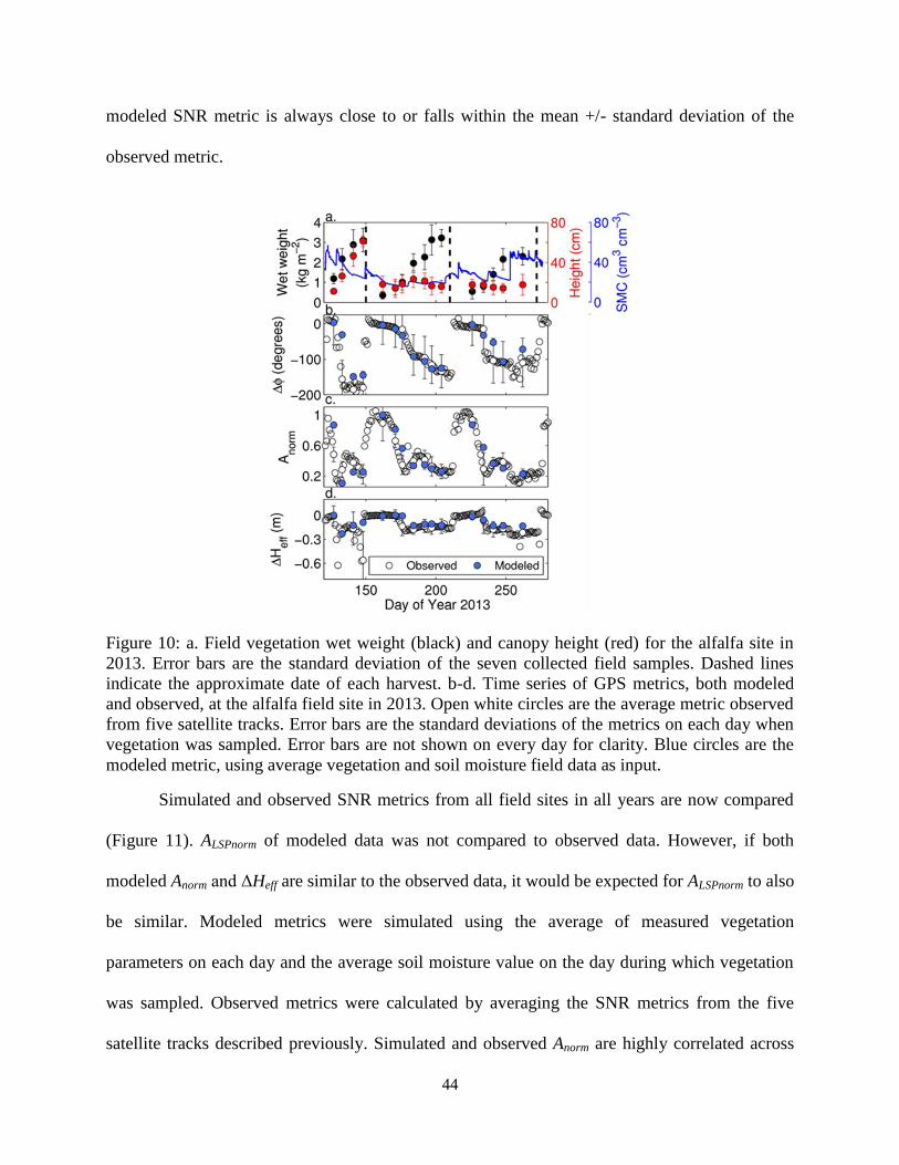
44
modeled SNR metric is always close to or falls within the mean +/- standard deviation of the
observed metric.
Figure 10: a. Field vegetation wet weight (black) and canopy height (red) for the alfalfa site in
2013. Error bars are the standard deviation of the seven collected field samples. Dashed lines
indicate the approximate date of each harvest. b-d. Time series of GPS metrics, both modeled
and observed, at the alfalfa field site in 2013. Open white circles are the average metric observed
from five satellite tracks. Error bars are the standard deviations of the metrics on each day when
vegetation was sampled. Error bars are not shown on every day for clarity. Blue circles are the
modeled metric, using average vegetation and soil moisture field data as input.
Simulated and observed SNR metrics from all field sites in all years are now compared
(Figure 11). ALSPnorm of modeled data was not compared to observed data. However, if both
modeled Anorm and ΔHeff are similar to the observed data, it would be expected for ALSPnorm to also
be similar. Modeled metrics were simulated using the average of measured vegetation
parameters on each day and the average soil moisture value on the day during which vegetation
was sampled. Observed metrics were calculated by averaging the SNR metrics from the five
satellite tracks described previously. Simulated and observed Anorm are highly correlated across

45
the entire range of observed vegetation wet weight (0-5 kg m-2
), with an r2 value of 0.79 and
root-mean-square error (RMSE) of 0.12. The r2 value between modeled and observed values of
Δϕ is also very high (0.84), and the RMSE is 20 degrees. ΔHeff has the lowest r2
of the three
metrics, with a value of 0.62 and RMSE of 0.09 m. This is likely due to the fact that, when there
high vegetation, there are sometimes two very prominent reflector heights shown in the LSP,
which compete to be the dominant frequency. Small adjustments in vegetation input would cause
one reflector height to be slightly more powerful than the other, causing apparent jumps in ΔHeff
time series.
Figure 11: Observed versus modeled SNR metrics, which includes data from all four field sites.
Points are colored by the observed vegetation wet weight, which was used as model input.
Observed metrics are the average, for a given day, of the metrics calculated using five satellite
tracks. Modeled metrics are created using the average vegetation field parameters collected on
that day. There is the same number of points in each panel. Many of the points in the ΔHeff plot
are clustered around zero.

46
4.3 Bare Soil Modeling
4.3.1 Soil moisture profiles
Now that the soil and vegetation model has been validated, relationships between soil and
vegetation input parameters and SNR metrics are quantified. This section assumes that the
environment surrounding a GPS antenna is devoid of vegetation. Here, contribution of only soil
moisture change to subsequent changes in SNR metrics is quantified. For this analysis, soil
moisture profiles that are constant with depth as well as ‘wetting’ or ‘drying’ profiles are
simulated in the model. These profiles are depicted in Figure 12a. In these profiles, soil moisture
was constant below 5 cm. The model was also run with soil profiles that had moisture variations
with depth down to 10 cm, but no significant differences were found compared with results from
the above profiles. It was thus deemed reasonable to keep soil moisture values constant below 5
cm depth. For profiles that vary with depth, the surface volumetric soil moisture value is denoted
as SM0, and the average volumetric soil moisture value for the top 5 cm of soil is denoted as
SM0-5.

47
Figure 12: (a) Simulated soil moisture profiles. Only the top 7 cm of the profiles are shown, as
soil moisture values were constant below 5 cm depth. (b) Relationship between ϕ and soil
moisture averaged over the top 5 cm, SM0-5. The unmarked line indicates results for profiles in
which soil moisture did not vary with depth. For these cases, the surface soil moisture is equal to
SM0-5. Other data (lines with symbols) are grouped by the value of soil moisture at the surface,
SM0. Within each group, each point corresponds to one profile in (a). The inset provides an
example of one group of profiles with the same surface soil moisture (0.15 cm3 cm
-3), taken from
(a). (c) Relationship between amplitude and soil moisture averaged over the top 5 cm, SM0-5. The
unmarked line indicates results for profiles in which soil moisture did not vary with depth. Other
data (lines with symbols) are grouped by the value of soil moisture at the surface, as in (b). (d)
Relationship between effective reflector height, Heff, and volumetric soil moisture averaged over
the top 5 cm, SM0-5. The unmarked line indicates results for profiles in which soil moisture did
not vary with depth. Other data (lines with symbols) are grouped by the value of soil moisture at
the surface, as in (b).
In addition to the theoretical wetting, drying, and depth-invariant soil moisture profiles,
in situ soil moisture data from the unirrigated agricultural wheat field (bcwh, see 3.1.1.1 and
3.2.2) were used to provide a representation of a set of realistic soil moisture profiles (Figure
13a). The data used to generate these profiles were collected using eleven Campbell Scientific
616 water content reflectometers: five were buried at a depth of 2.5 cm, five at 7.5 cm, and one
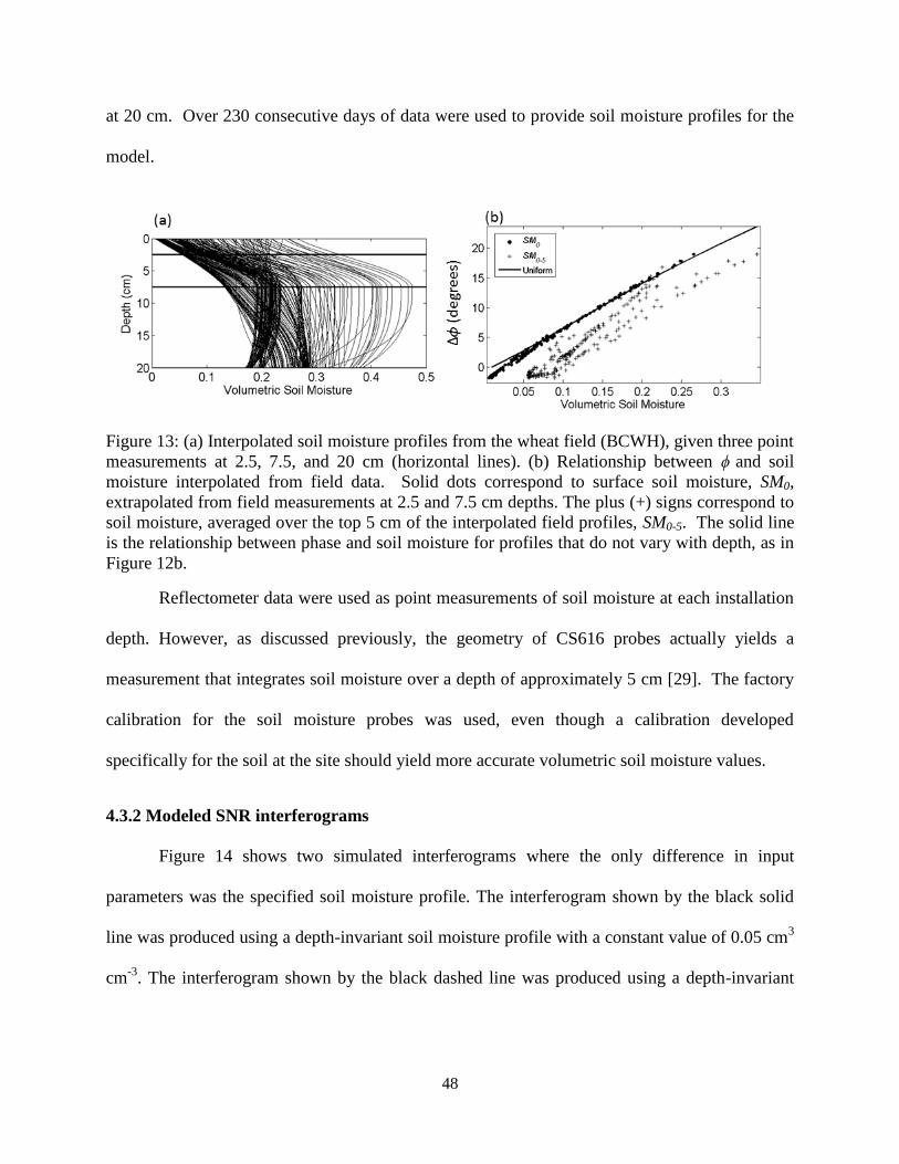
48
at 20 cm. Over 230 consecutive days of data were used to provide soil moisture profiles for the
model.
Figure 13: (a) Interpolated soil moisture profiles from the wheat field (BCWH), given three point
measurements at 2.5, 7.5, and 20 cm (horizontal lines). (b) Relationship between ϕ and soil
moisture interpolated from field data. Solid dots correspond to surface soil moisture, SM0,
extrapolated from field measurements at 2.5 and 7.5 cm depths. The plus (+) signs correspond to
soil moisture, averaged over the top 5 cm of the interpolated field profiles, SM0-5. The solid line
is the relationship between phase and soil moisture for profiles that do not vary with depth, as in
Figure 12b.
Reflectometer data were used as point measurements of soil moisture at each installation
depth. However, as discussed previously, the geometry of CS616 probes actually yields a
measurement that integrates soil moisture over a depth of approximately 5 cm [29]. The factory
calibration for the soil moisture probes was used, even though a calibration developed
specifically for the soil at the site should yield more accurate volumetric soil moisture values.
4.3.2 Modeled SNR interferograms
Figure 14 shows two simulated interferograms where the only difference in input
parameters was the specified soil moisture profile. The interferogram shown by the black solid
line was produced using a depth-invariant soil moisture profile with a constant value of 0.05 cm3
cm-3
. The interferogram shown by the black dashed line was produced using a depth-invariant

49
profile with a constant value of 0.45 cm3 cm
-3. Changing the input antenna height, H0, would
change the number of oscillations in each interferogram.
Figure 14: Two simulated interferograms, using either a constant soil moisture profile of 0.05
cm3 cm
-3 or 0.45 cm
3 cm
-3 as input. All other input parameters were the same between
simulations.
The interferogram simulated using the saturated soil moisture profile (dashed line) has a
lower amplitude than the interferogram simulated using the dry soil moisture profile (solid line)
except when sin(elevation angle) is greater than about 0.45. This is somewhat counterintuitive
because a higher soil moisture content should result in greater reflection and thus a greater
interference amplitude. However, reflection coefficients are both right- and left-handed circularly
polarized. The proportions of right- and left-handed polarization in the reflected wave depends
on soil moisture and the angle of incidence. Also, the gain pattern of the antenna accepts both
right- and left-handed polarizations differently depending on satellite elevation angle. These
complications make it difficult to predict SNR amplitude based solely on ground permittivity.

50
4.3.3 The effect of soil moisture on SNR metrics
4.3.3.1 Relationship between phase and soil moisture
Given uniform soil moisture profiles, ϕ exhibits a positive and nearly linear relationship
with volumetric soil moisture (Figure 12b). Phase varies by 30 degrees over the range of dry to
wet uniform soil moisture profiles that we tested. The slope of this relationship, or the sensitivity
of ϕ to uniform soil moisture, is 65.1 deg cm3 cm
-3. This means that a 20 degree change in ϕ
would correspond to a 0.31 change in volumetric soil moisture. This relationship is the same
regardless of soil type and does not depend on the height of the antenna, H0 (Table 5).
Table 5: Slopes and r2 values for linear regressions of soil moisture and phase using different soil
types for H0 = 2.4 m. Linear regressions assume soil moisture profiles do not vary with depth.
For soil moisture profiles that vary with depth, ϕ does not vary consistently with SM0-5.
Figure 12b shows the relationship between SM0-5 and ϕ for a variety of different soil moisture
profiles, a subset of which are depicted in the inset. The subset of profiles, labeled a-k in the
figure, all have the same surface volumetric soil moisture (0.15 cm3 cm
-3). However, the
volumetric soil moisture beneath the surface may be lower (profiles a-c) or higher (e-k) than at
the surface. As a result, these profiles have different values of SM0-5. As can be seen in the
figure, the relationship between SM0-5 and ϕ for these profiles is not linear, and the slope is much
smaller than that for uniform moisture profiles. This is true for the other groups of profiles that
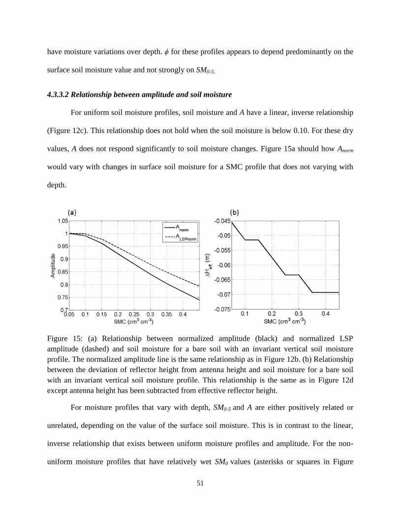
51
have moisture variations over depth. ϕ for these profiles appears to depend predominantly on the
surface soil moisture value and not strongly on SM0-5.
4.3.3.2 Relationship between amplitude and soil moisture
For uniform soil moisture profiles, soil moisture and A have a linear, inverse relationship
(Figure 12c). This relationship does not hold when the soil moisture is below 0.10. For these dry
values, A does not respond significantly to soil moisture changes. Figure 15a should how Anorm
would vary with changes in surface soil moisture for a SMC profile that does not varying with
depth.
Figure 15: (a) Relationship between normalized amplitude (black) and normalized LSP
amplitude (dashed) and soil moisture for a bare soil with an invariant vertical soil moisture
profile. The normalized amplitude line is the same relationship as in Figure 12b. (b) Relationship
between the deviation of reflector height from antenna height and soil moisture for a bare soil
with an invariant vertical soil moisture profile. This relationship is the same as in Figure 12d
except antenna height has been subtracted from effective reflector height.
For moisture profiles that vary with depth, SM0-5 and A are either positively related or
unrelated, depending on the value of the surface soil moisture. This is in contrast to the linear,
inverse relationship that exists between uniform moisture profiles and amplitude. For the non-
uniform moisture profiles that have relatively wet SM0 values (asterisks or squares in Figure

52
12c), A does not vary with SM0-5. For the profiles with lower SM0 (circles or ‘x’s in Figure 12c),
A is positively related to SM0-5. As is the case for ϕ, it appears that amplitude also depends
primarily on surface soil moisture, not SM0-5.
Figure 15a shows the relationship between amplitude and soil moisture for a constant soil
moisture profile for the more general case when amplitude is normalized with respect to its
maximum value. This figure also shows the relationship between normalized LSP amplitude
(ALSPnorm) and soil moisture for a constant soil moisture profile. Normalized LSP amplitude is not
affected by soil moisture as much as normalized amplitude calculated using the constant
frequency assumption, though the relationship does have the same general shape.
4.3.3.3 Relationship between effective reflector height and soil moisture
For uniform moisture profiles, as the soil becomes wetter the height estimated from the
Lomb-Scargle Periodogram (Heff) decreases (Figure 12d). The variation in Heff is approximately
3.3 cm for the range of soil moisture values tested.
As with both ϕ and A, once soil moisture profiles are allowed to vary with depth, the
dependence of Heff on SM0-5 is neither strong nor consistent. As is seen in Figure 12d, Heff varies
by < 1 cm with SM0-5 for moisture profiles that vary with depth. Thus, Heff appears to be
primarily influenced by SM0. The millimeter differences in Heff that result from moisture
variations at depth would be difficult to distinguish in field measurements. However, the cm-
level changes between uniform wet and dry profiles should be observable, as previously shown
by [14] and [15].
Figure 15b shows the same relationship as in Figure 12d for effective reflector height and
soil moisture, for a constant soil moisture profile with depth, though here antenna height, H0, has

53
been subtracted from Heff, yielding ΔHeff. Because the ground surface is not a perfect reflector,
there will be a frequency change upon reflection, resulting in the dominant frequency of the LSP
being different from that of the height of the antenna. In soil moisture simulations, the effective
reflector height is always lower than the actual input antenna height.
4.3.3.4 Relationship between metrics and SMC from field data
Here, results are presented for SNR data that were simulated using soil moisture profiles
interpolated from field data. SM0 and ϕ have a near-perfect correlation with an r2
value of 0.997
(Figure 13b) despite the wide range of soil moisture profiles tested. This indicates that ϕ is highly
dependent on changes in surface soil moisture. The correlation between ϕ and SM0-5 is still
excellent (r2 = 0.91) (Figure 13b). However, some of this correlation is the result of the
covariance between SM0-5 and SM0 rather than the effects of soil moisture at depth on SNR. Soil
moisture at 0 cm was extrapolated from the value measured at 2.5 cm using the gradient
measured at depths of 2.5 and 7.5 cm. Thus, the predicted SM0 was always tightly coupled with
this gradient. The covariance between SM0 and the soil moisture at deeper depths may not be as
strong in the field. Nearly all of the interpolated profiles have dryer soil at the surface than at
depth. Therefore, each ϕ -SM0-5 point plots to the right of the corresponding ϕ -SM0 point. This is
consistent with results shown in Figure 12a (e.g., points e-k), for cases when the soil is drier at
the surface than at depth.
A and Heff have similar correlations with the soil moisture profiles that were interpolated
from field measurements. The r2 value for the correlation between A and SM0 is 0.81 and 0.63 for
the correlation between A and SM0-5. The smaller r2
(compared to that for ϕ and soil moisture) is
expected, given the complex relationship between A and soil moisture (Figure 12c). The r2 value
for the correlation between Heff and SM0 is 0.97; between Heff and SM0-5, it is 0.86.

54
4.3.3.5 Note on signal penetration depth
It is well known that L-band signals penetrate further into soils that are dry than soils that
are wet [31]. It is possible to calculate the effective penetration depth, which is usually defined
as the depth at which the signal’s power has been attenuated to 1/e of its value at the soil surface
[31]. For passive L-band remote sensing, this depth varies from 0.1-1 m, depending on whether
the soil is wet or dry [31].
This definition of penetration depth, however, is not appropriate for defining the depth of
soil that significantly affects SNR. The signal may penetrate to this depth in the soil. However,
this does not mean that a significant portion of the signal returns back through the soil surface to
the antenna. In addition, SNR depends not only upon the depth at which the wave was reflected
but also on the dielectric properties of the soil. Other studies have also addressed this issue
[31][32]. The term for the region of soil that affects the overall signal is sometimes referred to as
the “moisture sensing depth” and is often taken to be one-tenth of a wavelength in the soil, which
corresponds to less than 2 cm for L-band [31].
Figure 13b indicates that the surface soil moisture value (top ~1 mm) is the determining
factor in ϕ. This is to be expected, since low elevation angles have higher surface reflection
coefficients than higher angles [28]. It appears that the observed correlations between ϕ and soil
moisture averaged over the top 5 cm of soil, like those shown in Figure 12b, result from a
combination of (1) strong covariance between SM0 and soil moisture at 2.5 cm and (2) soil
moisture at deeper depths affecting the overall signal. Although the relative contributions of
these two factors were not quantitatively compared, results show that the correlation between
SM0 and soil moisture at 2.5 cm is the driving factor in the correlation between the GPS
interferogram metrics A, Heff, and ϕ and SM0-5.
55
4.4 Vegetation-soil model
With the exception of deserts and plowed agricultural fields, there are few examples of
environments that are completely devoid of all vegetation. In natural environments, there is
almost always some amount of standing biomass, even in winter. It is thus important to quantify
the contribution of vegetation to changes in SNR metrics.
Observed SNR metric time series show significant variations in all metrics during times
of seasonal vegetation change (Figure 16). Figure 16 shows field vegetation and soil moisture
data collected from a GPS station in Oklahoma (OKL3) along with SNR metric time series from
that station. There are a few important things to note from this figure. One, the vegetation field
data show that the site is spatially heterogeneous, indicated by the large error bars in some of the
samples. Two, the vegetation field data do not show the same magnitude of change during the
summers of 2011 and 2012 (The site was burned in the winter of 2012.). Three, the SNR data
from different satellite tracks (indicated by the different colors in Figure 16) show wide ranges of
responses in every metric. Four, there is significant seasonality in the amplitude and phase time
series. Seasonality in the effective reflector height time series is not as apparent. And five, there
are smaller frequency oscillations in the phase time series that correspond with rain events and
subsequent dry downs.

56
Figure 16: In situ vegetation and soil moisture data for a GPS station in Oklahoma (OKL3) and
associated changes in SNR metrics for the same time interval. SNR metrics from different
satellite tracks are indicated by different colors.
It is clear from Figure 16 that SNR metrics are affected by seasonal variations in land
surface characteristics. The goal of this section is to identify and quantify the most important
parameters controlling the seasonal changes in SNR metric time series using the soil-vegetation
model. This section will also address how concurrent changes in soil moisture and overlying
vegetation lead to complicated responses in SNR metrics.
The soil-vegetation model is able to reproduce the changes in the shape of SNR
interferograms as well as changes in associated metrics due to changes in a vegetation canopy, as

57
shown in Figure 9. I will now address what vegetation and soil parameters are most important in
affecting metrics.
I will start with the most general case, which is how random combinations of the
vegetation parameters in Table 6 affect SNR metrics. I will then present how assigning
relationships between vegetation parameters affects our results. In addition, the role of changing
underlying soil moisture will be discussed.
Table 6: Parameters used in the soil-vegetation model
4.4.1 First case: random combinations of vegetation parameters
Here, vegetation parameters, specifically Mf, Md, Hveg, and ρveg, are varied randomly, and
combinations of the random parameters are used as input to the model. Antenna height and
vegetation salinity are held constant, and soil moisture is kept at 0.15 cm3 cm
-3. Some bounds are
placed on parameters, such that Mf must be under 3 kg m-2
, Md is under 1.5 kg m-2
, Hveg is under
80 cm, and ρveg is between 200-1500 kg m-3
. Approximately 10,000 model simulations were run

58
with random combinations of these parameters, and SNR metrics were calculated. Anorm, ALSPnorm,
ΔHeff, and Δϕ were calculated using the bare soil case (SMC = 0.15 cm3 cm
-3) as a reference from
which to normalize and zero metrics. In these simulations, ΔHeff is defined as the change in
effective reflector height with respect to its value during times when soil is essentially ‘bare.’
Note that this is slightly different than how it would normally be defined in the model, when the
a priori reflector height is perfectly known.
Figure 17-Figure 20 show the relationships between the vegetation parameters in the
model and corresponding SNR metrics. Figure 17, which shows how metrics vary with the dry
biomass of vegetation (Md), indicates very weak relationships with all metrics. An increase in dry
biomass in general causes a decrease in Anorm, ALSPnorm, and Δϕ. Also, an increase in dry biomass
causes Heff to decrease with respect to its bare soil value, indicated by the positive values of ΔHeff.
The small cloud of outliers in the ΔHeff plot is caused by a second, competing frequency in the
LSP that will sometimes be the most powerful frequency. This is discussed in more detail below.
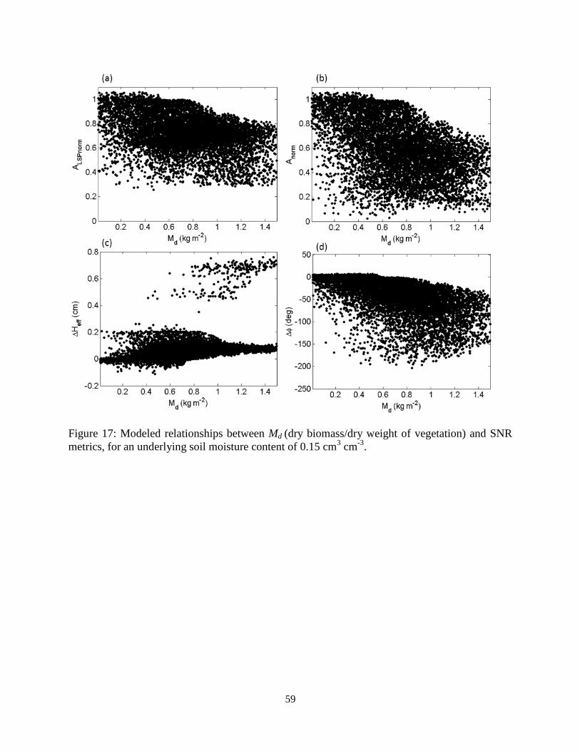
59
Figure 17: Modeled relationships between Md (dry biomass/dry weight of vegetation) and SNR
metrics, for an underlying soil moisture content of 0.15 cm3 cm
-3.

60
Figure 18: Modeled relationships between Mf (fresh biomass/wet weight of vegetation) and SNR
metrics, for an underlying soil moisture content of 0.15 cm3 cm
-3.

61
Figure 19: Modeled relationships between Hveg (height of vegetation canopy) and SNR metrics,
for an underlying soil moisture content of 0.15 cm3 cm
-3.

62
Figure 20: Modeled relationships between ρveg (true density of vegetation) and SNR metrics, for
an underlying soil moisture content of 0.15 cm3 cm
-3.
Figure 18 shows the relationship between the wet weight/fresh biomass of vegetation
(Mf) and SNR metrics. Like Md, Mf also causes SNR metrics to decrease. The relationship
between Mf and the amplitude metrics is clearer than that for Md, though there is still significant
scatter. There do not appear to be significant differences between the relationships of Mf, Md and
Δϕ, ΔHeff.
Changes in vegetation canopy height result in very different changes in SNR metrics than
changes in fresh or dry biomass (Figure 19). Vegetation canopy growth from bare soil to 14 cm
results in only very small changes in SNR metrics, relative to larger changes in vegetation

63
height. Beyond 14 cm, changes in canopy height could result in significant decreases in all SNR
metrics, or result in no changes. This is a good indication that changes in SNR metrics are
controlled by the interaction between multiple canopy parameters. When the canopy height is
between 20 and 50 cm, SNR amplitude metrics could actually begin to increase again, depending
on the value of other parameters, which will be explored below. In general, the relationship
between changes in canopy height and ΔHeff are not 1:1, except for a small number of cases. This
will also be discussed in more detail below.
Figure 20 shows how SNR metrics are affected by changes in the true density of
vegetation. True density is weakly associated with amplitude and phase metrics, with an increase
in true density resulting in increases in Δϕ, Anorm, and ALSPnorm. There is no obvious relationship
between changes in true density and changes in ΔHeff.
Now that the relationships between changes in single vegetation parameters and SNR
metrics has been presented, it is apparent that SNR metrics are affected by changes in not just
one, but multiple, vegetation parameters. Combining vegetation parameters into a single
parameter, the effective canopy permittivity, yields better relationships with SNR metrics, and
the combination of canopy height and permittivity yields the best relationships. Presenting
results in terms of canopy permittivity also makes sense because reflection coefficients are
calculated using the permittivity value—not any individual vegetation parameter.
How Anorm is affected by changes in canopy permittivity and canopy height is shown in
Figure 21a. For low values of canopy permittivity (<1.04), an increase in canopy height will not
affect Anorm. When canopy permittivity is higher than 1.04, an increase in canopy height will
cause a general decrease in Anorm. Depending on the specific plant type, canopy height and

64
permittivity could be correlated at part or all of its growth cycle, which means an increase in
either one would cause a decrease in Anorm.
Figure 21: Relationships between canopy permittivity (real part), canopy height, and SNR
metrics. Underlying soil moisture was kept at 0.15 cm3 cm
-3.
Figure 21b shows the relationship between ALSPnorm, canopy height, and permittivity.
ALSPnorm is affected by canopy height and permittivity somewhat similarly as Anorm, with some
notable exceptions. For low values of canopy permittivity or low values of canopy height, both
ALSPnorm and Anorm respond similarly. However, for some combinations of canopy height and
permittivity, ALSPnorm may increase substantially for a period of time (again, depending on the
particular plant’s growth strategy). This increase is likely due to the growth of a second dominant
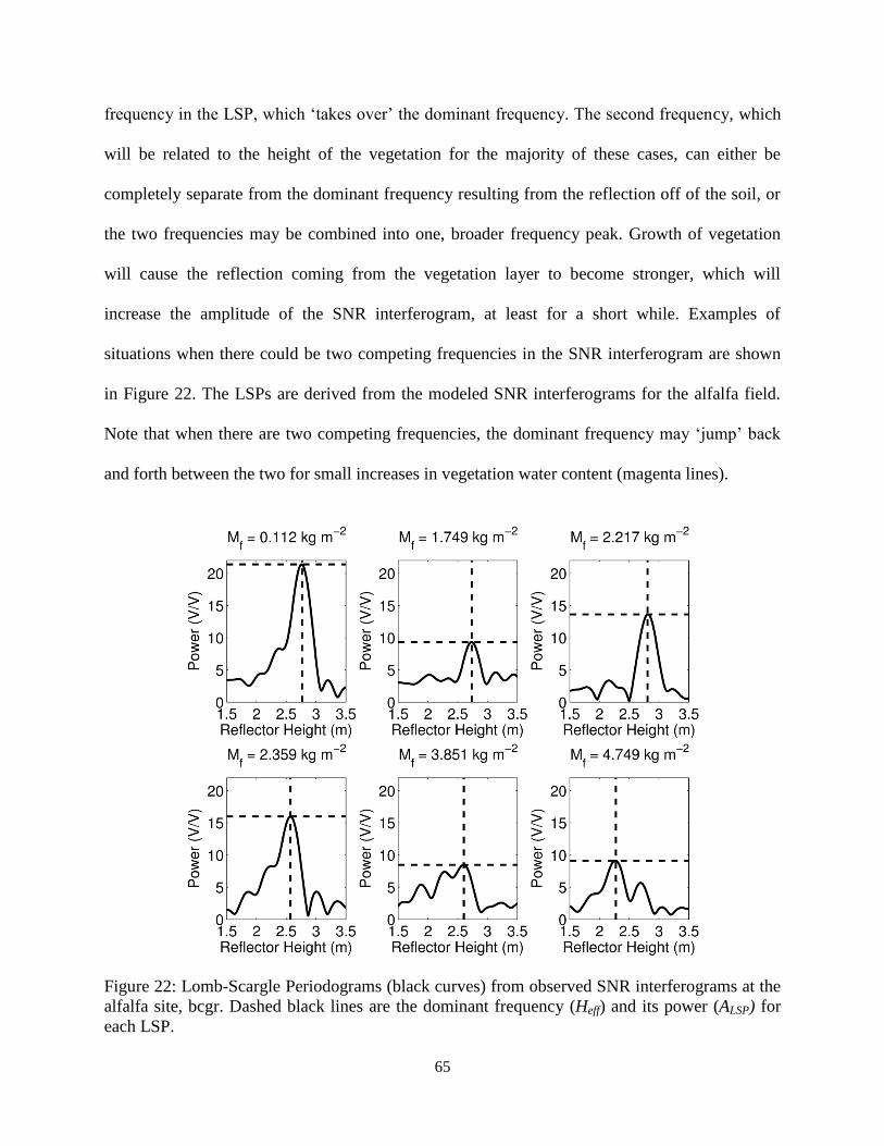
65
frequency in the LSP, which ‘takes over’ the dominant frequency. The second frequency, which
will be related to the height of the vegetation for the majority of these cases, can either be
completely separate from the dominant frequency resulting from the reflection off of the soil, or
the two frequencies may be combined into one, broader frequency peak. Growth of vegetation
will cause the reflection coming from the vegetation layer to become stronger, which will
increase the amplitude of the SNR interferogram, at least for a short while. Examples of
situations when there could be two competing frequencies in the SNR interferogram are shown
in Figure 22. The LSPs are derived from the modeled SNR interferograms for the alfalfa field.
Note that when there are two competing frequencies, the dominant frequency may ‘jump’ back
and forth between the two for small increases in vegetation water content (magenta lines).
Figure 22: Lomb-Scargle Periodograms (black curves) from observed SNR interferograms at the
alfalfa site, bcgr. Dashed black lines are the dominant frequency (Heff) and its power (ALSP) for
each LSP.

66
How ΔHeff is affected by canopy permittivity and height is presented in Figure 21c. For a
large portion of the permittivity/canopy height parameter space, ΔHeff does not change more than
20 cm. For very tall canopies with high permittivities, ΔHeff is strongly correlated with canopy
height, with second-order effects from changes in permittivity.
Figure 21d shows how height and permittivity affect Δϕ. Changes in Δϕ are generally
restricted to less than 200 degrees for the canopies simulated here. The small region with
changes larger than 360 (dark blue) resulted from inadequate phase zeroing. In almost all cases,
phase will decrease due to a combination of permittivity and height increases, unlike ALSPnorm.
4.4.2 Second case: Assuming relationships between canopy parameters
As mentioned above, SNR metrics will respond differently to plants with different
growth strategies. To illustrate differences, I will present examples using vegetation field data
from mfle and bcgr (the desert steppe and alfalfa sites). For these examples, I derived general
empirical relationships between vegetation canopy parameters for each site and used these
relationships in model simulations.
Empirically derived relationships are shown in Figure 23. Figure 23a shows how, at each
site, biomass varies with water content. Each data point is the average from one field survey. The
vegetation at the desert steppe site does not vary as much as the vegetation at the alfalfa site. The
vegetation at the desert steppe site is also much drier, as indicated by the smaller slope between
biomass and water content. The linear regressions for each site are shown by the dashed lines—
this relationship is strong for both sites. Figure 23b shows how canopy height varies with
biomass. Relationships are not as strong, though linear regressions are still shown.
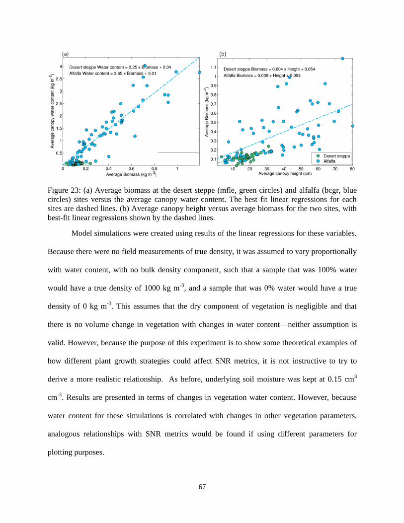
67
Figure 23: (a) Average biomass at the desert steppe (mfle, green circles) and alfalfa (bcgr, blue
circles) sites versus the average canopy water content. The best fit linear regressions for each
sites are dashed lines. (b) Average canopy height versus average biomass for the two sites, with
best-fit linear regressions shown by the dashed lines.
Model simulations were created using results of the linear regressions for these variables.
Because there were no field measurements of true density, it was assumed to vary proportionally
with water content, with no bulk density component, such that a sample that was 100% water
would have a true density of 1000 kg m-3
, and a sample that was 0% water would have a true
density of 0 kg m-3
. This assumes that the dry component of vegetation is negligible and that
there is no volume change in vegetation with changes in water content—neither assumption is
valid. However, because the purpose of this experiment is to show some theoretical examples of
how different plant growth strategies could affect SNR metrics, it is not instructive to try to
derive a more realistic relationship. As before, underlying soil moisture was kept at 0.15 cm3
cm-3
. Results are presented in terms of changes in vegetation water content. However, because
water content for these simulations is correlated with changes in other vegetation parameters,
analogous relationships with SNR metrics would be found if using different parameters for
plotting purposes.

68
Figure 24 shows how changes in vegetation water content for the scenarios described
above affect SNR metrics. One can think of this as theoretical changes in SNR metrics
throughout the growing season for the two different vegetation types. Figure 24a indicates that
both the desert steppe and alfalfa sites would see a slight increase in Anorm at the beginning of the
growing season, followed by sharp decreases. The decrease in Anorm would be more significant at
the beginning of the desert steppe’s growth cycle relative to alfalfa, but much shorter lived.
Figure 24: (a) Modeled decreases in Anorm at the desert steppe (green) and alfalfa (blue) sites as
vegetation water content increases. (b) Modeled effect of vegetation water content on ALSPnorm at
the desert steppe and alfalfa sites. (c) Modeled effect of vegetation water content on ΔHeff at the
desert steppe and alfalfa sites. (d) Modeled effect of vegetation water content on Δϕ at the desert
steppe and alfalfa sites.
69
Figure 24b, which shows how ALSPnorm varies with vegetation water content, indicates that
for the desert steppe site, ALSPnorm and Anorm are virtually the same. At the alfalfa site, however,
there is an increase and subsequent decrease in ALSPnorm from 1.5-2.5 kg m-2
, which is much
larger than the effect seen in Anorm.
There is hardly any change in ΔHeff at the desert steppe site (Figure 24c). Conversely,
there are large step changes in ΔHeff as vegetation water content increases at the alfalfa site.
These step changes are also indicated in Figure 21c as well. These step changes are caused by
two or more frequencies in the SNR interferogram that compete to be the dominant frequency.
The effect of increasing vegetation water content on Δϕ is shown in Figure 24d. The
effect is very similar to both Anorm and ALSPnorm—the desert steppe site shows a faster decrease of
phase for low increases in water content than the alfalfa site. Δϕ does show a small increase at 2
kg m-2
at the alfalfa site, though there is no intermittent increase/decrease effect as in the
amplitude data.
4.4.3 Third case: When specific vegetation parameters are correlated with one another
The example above shows very specific cases for when the relationships between all
vegetation parameters are linear and known. However, in real field settings these relationships
are never known with 100% certainty, as indicated by the significant scatter in Figure 23. In
addition, most PBO sites have little to no vegetation data. Even sites that do have data will be
expected to vary substantially from year to year. Thus, although the above example is instructive
for showing how different the response of metrics to vegetation may be at two different sites, it
cannot be used practically. A slightly less specific example, though still more specific than when
vegetation parameters are completely unknown, is now presented.

70
For these simulations, vegetation wet weight (Mf) was allowed to vary between 0-4 kg
m−2
, canopy height (Hveg) between 1-100 cm, and vegetation percent water content (from which
one can infer dry biomass) between 10-90%. Parameter sets which resulted in permittivites
higher than 1.1 were excluded from the final analysis. The primary difference between these
simulations and the completely random simulations described previously is in the treatment of
vegetation true density, ρveg, which now is set to be directly proportional to its water content, as
in the desert steppe/alfalfa simulations above. Here, underlying soil moisture was 0.05 cm3 cm
-3
in our ‘dry’ library. An identical library of vegetation model simulations for ‘wet’ conditions was
also created, in which soil moisture was 0.4 cm3 cm
-3. This allowed investigation of how
changing soil moisture beneath a vegetation canopy will affect SNR metrics. ALSPnorm was not
calculated for these model simulations, as they were completed before this metric was
recognized as being potentially valuable in vegetation estimation.
Figure 25 shows how changes in vegetation wet weight (Mf) affects SNR metrics for
these simulations. Each model simulation is colored by its canopy height. Notably in Fig. 34a
(bottom), it appears that even at high values of vegetation wet weight, differences in canopy
height can significantly change Δϕ. Canopy height does not change the relationship between wet
weight and Anorm as drastically, as shown in Figure 25b (bottom). There are similar step changes
in ΔHeff (Figure 24c) as in the simulations modeling the alfalfa field.

71
Figure 25: Model SNR metrics using random combinations of vegetation parameters and a dry
(0.05) soil moisture profile as input. Metrics are plotted against modeled vegetation wet weight
and colored by modeled canopy height. a. (top) The absolute magnitude of phase change if a wet
(0.40) soil moisture profile were used as input. The range of the box is the same as the range in
the box below. The subscript SMC is used to denote that the phase change is from soil moisture
only. (bottom) The relationship between phase and vegetation wet weight for random model
simulations with the dry soil moisture profile. b. (top) The absolute magnitude of normalized
amplitude change if a wet (0.40) soil moisture profile were used as input. The range of the box is
the same as the range in the box below. The subscript SMC is used to denote that the amplitude
change is from soil moisture only. (bottom) The relationship between normalized amplitude and
vegetation wet weight for random model simulations with the dry soil moisture profile. c. The
relationship between change in effective reflector height and vegetation wet weight for random
model simulations with the dry soil moisture profile.
4.4.4 Effects of underlying soil moisture changes
The above three scenarios describe how vegetation affects SNR metrics, and section 4.3
showed how fluctuations in soil moisture for a bare surface changed SNR metrics. This section
describes how concurrent changes in both soil moisture and vegetation obfuscate much of what
was stated above (but don’t worry, you didn’t completely waste your time by reading the
previous two sections!). Temporal changes in each SNR metric are some combination of changes
of that metric from soil moisture and changes from vegetation. The simplest of combinations

72
would be if the total change of a metric were a linear combination of the two contributors, i.e.
total phase change is the summation of the phase change due to vegetation and the phase change
due to soil moisture.
We will now investigate whether or not this is the case, first by showing how changing
soil moisture would affect conclusions drawn from the third scenario described in the previous
section. Figure 25 (a-b, top) indicates the change in phase or normalized amplitude if soil
moisture changes from 0.05 cm3 cm
-3 to 0.4 cm
3 cm
-3, for a given overlying vegetation canopy.
Here, I have plotted the absolute value of the change and scaled each box to the range of their
respective boxes below. I did not include the analogous panel for effective reflector height
because changes exceeded +/- 0.1 m, or 10% of the range, in only a handful of cases. Figure 25
(b, top) shows that the influence of soil moisture on Anorm is relatively small compared to the
influence of vegetation on this metric. The figure also shows that the influence of soil moisture
on normalized amplitude is relatively constant, compared to the Anorm changes expected from
vegetation.
If one were only worried about estimating vegetation changes using SNR metrics, using
Anorm as a proxy for vegetation change would have relatively small uncertainties introduced from
soil moisture variations. Figure 25 (a, top) shows that the case for Δϕ is different. The change in
phase due to soil moisture is approximately one third of that caused by vegetation for most of the
canopies tested. However, for short and dense canopies, Δϕ from soil moisture is roughly equal
to that from vegetation. This suggests that a large phase change could be due to either a change
in soil moisture or in vegetation, or concurrent changes in both.

73
The model simulates changes in both phase and amplitude from soil moisture across the
range of canopies tested here. Intuitively, one would expect a decrease in sensitivity to soil
moisture for denser vegetation canopies. This general effect is simulated by the model: the
influence of soil moisture on phase does generally diminish as permittivity increases. However,
the simulated vegetation canopy does not completely obscure soil moisture effects until the
canopy permittivity exceeds ~2.0 (not shown). The canopies tested here are primarily composed
of air, so the permittivity in almost always between 1.01 and 1.10. These permittivity values are
consistent with published values [56]. For these permittivity values, the vegetation canopy does
not completely obscure the underlying soil.
We now return to the original case of not having any a priori knowledge of vegetation at
the site. How does a change in soil moisture change our conclusions drawn from Figure 21? The
same combinations of randomized vegetation parameters as above were used to create additional
simulations, except the parameters were each paired with an underlying soil moisture of 0.05 cm3
cm-3
and 0.45 cm3 cm
-3. SNR metrics were recalculated. Then, for each modeled vegetation
canopy, the difference between metrics was calculated for the case when soil moisture was 0.45
cm3 cm
-3 and the case when soil moisture was 0.05 cm
3 cm
-3.
In other words, this experiment essentially shows how the slope between phase and soil
moisture will change as overlying vegetation changes. The sensitivity of phase to soil moisture
for the bare soil case was approximately 25 degrees, for typical ranges of possible moisture
contents. Figure 26d shows how the sensitivity of phase to soil moisture changes depending on
the vegetation canopy. For example, a change in soil moisture of 0.4 cm3 cm
-3 would result in a
phase change of approximately 25 degrees for a canopy with permittivity of 1.05 and height of
10 cm. However, the same soil moisture change would result in a greater than 50 degree phase

74
change if the permittivity were 1.1 and the height were 30 cm. Again, this is not intuitive.
Shouldn’t phase sensitivity to soil moisture decrease when either the height or permittivity of the
canopy increases?
Figure 26: Model simulations showing the relationship between vegetation canopy permittivity
(ɛcanopy), the height of the vegetation (Hveg), and how much (a) amplitude (b) LSP amplitude (c)
effective reflector height and (d) phase would respond to a change in soil moisture from 0.05 cm3
cm-3
to 0.45 cm3
cm-3
for the given vegetation canopy parameters. The amplitude metrics were
normalized with respect to the bare soil values at 0.15 cm3
cm-3
moisture content.
The difference between the frequency/a priori reflector height (H0) used to estimate
phase and amplitude and the actual frequency(cies)/effective reflector height(s) (Heff) of the SNR
data is largely, though not totally, responsible for the apparent increase in the response of phase
to soil moisture for some vegetation canopies, which is seen in Figure 26d. When the

75
discrepancy between H0 and Heff becomes large, the frequency that is used in least-squares
estimation of phase and amplitude is no longer characteristic of the actual data, and errors will be
introduced in their estimation. The apparent large response of phase to soil moisture changes for
these dense canopies is more reflective of the errors introduced by the frequency discrepancies in
least-squares estimation than in an actual phase response. However, assuming all other things
equal, these types of responses of phase to soil moisture should also be apparent in observed
data. Though, additional noise and other complexities found in real data could preclude this
effect.
Figure 26a-c show the sensitivity changes of other metrics to changes in soil moisture.
Figure 26a, which shows how Anorm responds to soil moisture beneath vegetation canopies, is
subject to the same errors as phase, in terms of inappropriate frequency assignment in least-
squares estimation. Figure 26b, which shows how ALSPnorm responds to soil moisture changes, is
also subject to analogous errors due to multiple strong ground- and canopy-reflections, though
mostly once the reflection coming from the canopy layer is strong enough to compete with the
reflection coming from the soil layer. Both amplitude metrics indicate that the amplitude value
may either decrease or increase from its bare soil value, depending on the vegetation canopy.
Figure 26c indicates that ΔHeff does not behave in the same way as the phase and
amplitude metrics do. There is not as apparent oscillatory behavior in its sensitivity to soil
moisture fluctuations. Large jumps in sensitivity are probably caused by the presence of a
second, competing frequency in the SNR data. For the most part, sensitivity of ΔHeff to soil
moisture fluctuations is between 0-2 cm.

76
4.4.5 Problems with the constant-frequency SNR equation
As briefly discussed earlier, SNR metrics are calculated under the assumption that the
SNR interferogram is comprised of a singular amplitude, phase, and frequency. Just looking at
an interferogram, it is apparent that at least the amplitude of the interferogram is not constant
with elevation angle. This is mostly due to the effect of the antenna’s gain pattern of the ground-
reflected signal. As Figure 9 shows, amplitude at different elevation angles increases or
decreases depending on the vegetation canopy. The LSPs shown in Figure 22 indicate that there
are situations in which there are multiple frequencies in the interferograms.
I have shown that SNR metrics are affected in nonlinear, complex ways due to concurrent
changes in soil moisture and vegetation. Part of these complicated interactions is due to the fact
that the SNR metrics themselves do not always describe the interferogram adequately. Using
least-squares with the constant-frequency characterization of (2) can be fraught with problems
when the actual data have non-constant amplitude and potentially multiple frequencies. What I
will show now is how the characteristic equation of SNR data (2) will sometimes mischaracterize
the actual data, particularly when there is high vegetation present.
One can visualize the mischaracterization of SNR data by plugging the estimated A and ϕ
values back into (2) and assuming that the frequency is a function of H0, the a priori reflector
height. Figure 27 shows how the SNR metrics from the model simulations in Figure 25 actually
characterize their respective interferograms. Here, model simulations have been plotted with
respect to their wet weight/Mf values, though they could have been plotted against another
parameter. I chose to quantify how well each modeled interferogram can be recreated using the
estimated SNR metrics from (2) alone using r2. In other words, I computed the r
2 value between
each interferogram and the interferogram that results from plugging in the SNR metrics into (2).

77
What we see is that as wet weight increases, the r2 value decreases non-linearly and significantly.
This confirms the suspicion that vegetation growth causes an increase in the mischaracterization
of the actual interferogram, due to the fact that the constant-frequency assumption in (2) is no
longer appropriate.
Figure 27: Results from random model simulations using the soil-vegetation model. The fresh
mass/wet weight of the model simulation is plotted against the r2 value between the simulated
interferogram, and the interferogram that would result if its estimated phase and amplitude were
used in Eq. (2).
It is apparent that assuming the dominant frequency of the SNR data is equal to the a
priori reflector height can oftentimes result in the mischaracterization of SNR data. The way
SNR data are characterized with the current SNR metrics is obviously a problem, though the way
this problem is addressed is discussed in later sections.
4.4.6 Conclusions
In summary, this chapter has explored the theoretical effects of both soil moisture and
vegetation canopy parameters on SNR interferograms and metrics. The model was first validated
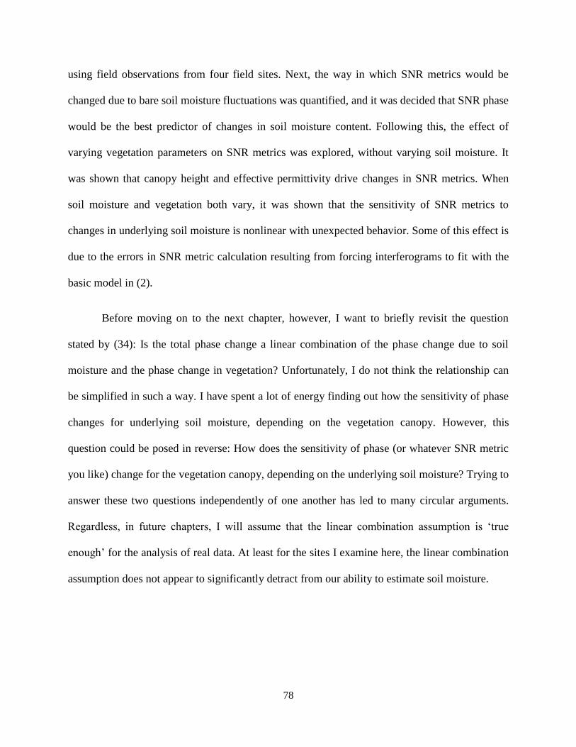
78
using field observations from four field sites. Next, the way in which SNR metrics would be
changed due to bare soil moisture fluctuations was quantified, and it was decided that SNR phase
would be the best predictor of changes in soil moisture content. Following this, the effect of
varying vegetation parameters on SNR metrics was explored, without varying soil moisture. It
was shown that canopy height and effective permittivity drive changes in SNR metrics. When
soil moisture and vegetation both vary, it was shown that the sensitivity of SNR metrics to
changes in underlying soil moisture is nonlinear with unexpected behavior. Some of this effect is
due to the errors in SNR metric calculation resulting from forcing interferograms to fit with the
basic model in (2).
Before moving on to the next chapter, however, I want to briefly revisit the question
stated by (34): Is the total phase change a linear combination of the phase change due to soil
moisture and the phase change in vegetation? Unfortunately, I do not think the relationship can
be simplified in such a way. I have spent a lot of energy finding out how the sensitivity of phase
changes for underlying soil moisture, depending on the vegetation canopy. However, this
question could be posed in reverse: How does the sensitivity of phase (or whatever SNR metric
you like) change for the vegetation canopy, depending on the underlying soil moisture? Trying to
answer these two questions independently of one another has led to many circular arguments.
Regardless, in future chapters, I will assume that the linear combination assumption is ‘true
enough’ for the analysis of real data. At least for the sites I examine here, the linear combination
assumption does not appear to significantly detract from our ability to estimate soil moisture.

79
Chapter 5: Correcting for vegetation effects on SNR data
This chapter addresses how the vegetation effect on SNR data is mitigated using
simulations generated from the soil and vegetation model described in Chapter 4.
5.1 Extent of vegetation effects in observed data
At a number of Plate Boundary Observatory (PBO) network GPS sites, the SNR data are
affected by both soil moisture change and seasonal vegetation growth cycles. One way that we
have estimated the extent of vegetation effects on SNR data is by looking at smoothed and
normalized SNR amplitude (Anorm) time series. [62] showed that Anorm is the SNR metric that is
affected predominantly by changes in vegetation, and to a lesser extent by soil moisture. We use
the amplitude time series as a proxy for changes in vegetation.
Figure 28 shows a histogram of Anorm values for all satellites tracks at all PBO H2O sites.
The dashed line shows an approximate cutoff where one can be reasonably certain that there are
significant changes in vegetation at the GPS site (Anorm = 0.78). The cutoff is an approximation
of how much Anorm would be expected to decrease when soil moisture content (SMC) increases
from residual to saturated values (Figure 15), though this cutoff would change for soil types that
could have larger or smaller SMC ranges. Figure 28 indicates that at least 20% of the data are
affected by vegetation. This is a minimum estimate, as higher Anorm values may still indicate
vegetation changes, depending on soil moisture changes.

80
Figure 28: Histogram showing the percentage of PBO H2O data that fall into normalized
amplitude bins. The dashed line indicates the point at which observations are significantly
affected by vegetation.
5.2 Development of the vegetation filter
As stated previously, an increase in vegetation amount could be mistaken for a decrease
in soil moisture in the phase time series. Before final soil moisture estimations may be made, the
SNR phase time series at the sites with relatively significant vegetation change must be cleaned,
or filtered, for vegetation effects. I will now describe the method used in the PBO H2O database
for filtering phase time series for vegetation.
The filter described here is a compromise between the need for accuracy, computational
efficiency, and generality for the variety of vegetation conditions found at the PBO sites. The
filter relies on the soil-vegetation model, described and validated in [62], to provide simulations
of how SNR metrics change with canopy height and permittivity changes (Figure 21), in the

81
absence of soil moisture change. Relationships between SNR metrics themselves, which result
from the vegetation changes, are used to clean the SNR phase time series. In other words,
changes in Anorm, ALSPnorm, and ΔHeff are used to predict changes in Δϕ from vegetation.
5.2.1 SNR model simulations
The SNR model simulations used in the vegetation filter are the result of pseudo-random
combinations of vegetation parameters. Parameter sets representing different vegetation canopies
needed to be realistic, but they also needed to be varied enough to encompass a wide range of
canopy possibilities. The final filter includes 16000 vegetation parameter sets meant to represent
both semi-dry natural environments as well as wetter agricultural fields, though a larger
proportion of simulations represent natural environments. Parameter sets that resulted in
vegetation canopies with an effective (real) permittivity of greater than 1.2 were excluded from
the filter. Figure 29 shows distributions of vegetation parameters used in the model simulations.
Figure 29: Distributions and ranges of vegetation parameters used in vegetation filter model
simulations. Fresh biomass or the wet weight of vegetation is denoted by Mf, dry biomass is
denoted by Md, canopy height by Hveg, and true density by ρveg. Vegetation salinity was kept at its
default value.

82
The model was run for these parameter sets assuming an underlying bare soil moisture
content of 0.15 cm3 cm
-3. I chose to use 0.15 cm
3 cm
-3 because it was a compromise between the
drier average SMC for desert or arid environments and the wetter average SMC for other sites,
like Oklahoma (Figure 6). Assuming different underlying moisture contents does in fact change
the filter—this is discussed below.
5.2.2 Relationships between SNR metrics
After the model simulations were created, SNR metrics were calculated. Once metrics
were calculated, it was necessary to then understand how Anorm, ALSPnorm, and ΔHeff could be used
to predict changes in Δϕ. Keep in mind that we are not actually trying to first estimate changes in
vegetation with the filter—we only want to discover how the relationships between metrics
themselves change due to changes in vegetation only.
Depending on the vegetation parameters, relationships between metrics themselves will
change. Examples are shown in Figure 30 which depicts how the relationship between different
metrics and phase will change depending on the vegetation canopy. It is apparent from Figure 30
that no one SNR metric, in the absence of abundant vegetation field data, can accurately predict
the change in phase. However, using the combination of SNR metrics can provide more accurate
predictions (Figure 31). Figure 31a shows how Anorm and ALSPnorm can be used together to predict
changes in phase due to vegetation. Once Anorm decreases to about 0.4, phase is not well-
predicted by changes in the two amplitude metrics. However, as Figure 31b shows, using
information contained in reflector height variations can help predict changes in phase past an
amplitude decrease beyond 0.4. It should be noted that the relationships between SNR metrics
and phase are not smoothly-varying when amplitudes are below 0.4 and reflector height has not

83
changed by more than 10 cm (Figure 31b). One would thus expect more error in phase
predictions in these situations.
Figure 30: The relationships between SNR metrics and Δϕ, which vary depending on vegetation
parameters. Here, points are colored by canopy permittivity (real part).
5.3 Processing observed SNR metrics
Because soil moisture changes will affect all SNR metrics to different degrees, the
observed LSP amplitude, amplitude, and reflector height time series are first smoothed before
being used in the filter (examples shown in Figure 32). Smoothing the time series means that we
are assuming that long-term changes in the SNR metrics are only due to vegetation change and
not due to long-term (i.e., seasonal) changes in surface soil moisture. Despite this, I have found

84
that the filter does a sufficient job at preserving the longer term soil moisture signals, at least at
our validation sites in Oklahoma.
The choice of a smoothing method is relatively important due to the fact that changes in
vegetation may occur rapidly at a site. Moving mean and median filters are sometimes
successful, though occasionally they can over-smooth rapid vegetation growth and senescence.
For very small vegetation changes, a moving mean or median is probably sufficient, though in
these cases the necessity of the vegetation filter itself is questionable.
Using a Savitzky-Golay filter has shown to be more successful at preserving the timing
and magnitude of vegetation growth and senescence while still being relatively insensitive to
noise. A Savitzky-Golay filter fits subsets of adjacent data points with low-order polynomials
using least-squares. The parameters needed for the filter have been found to be important in
smoothing the SNR metric time series. In the current version of the vegetation filter, a
polynomial order of 4 and data span of 63 days is used to smooth each time series. The filter is
least successful in smoothing reflector height time series due to the relatively high proportion of
noise to long-term change.
5.4 Estimating phase change due to vegetation
As it was shown in Figure 30 and Figure 31, the effect of vegetation on the relationship
between SNR metrics is complicated without obvious functional relationships. For this reason,
the SNR metrics derived from the model simulations are saved in a data cube or lookup table. An
observed triplet of Anorm, ALSPnorm, and Heff (after smoothing) is compared to the triplets contained
in the metric lookup table. A linear nearest neighbor search algorithm is used to find the best-
matching modeled triplet and its associated phase change. Although generally computationally

85
inefficient for large data sets, the search algorithm does not take significantly long for the
modeled data set used in the vegetation filter.
Figure 31: (a) Relationship between Anorm, ALSPnorm, and Δϕ, for the simulations used in the
vegetation filter. (b) Same relationships as in (a) except also with ΔHeff.
Predicted phase changes due to vegetation are also smoothed to mitigate noise introduced
by the linear nearest neighbor search algorithm. The predicted phase change due to vegetation,
Δϕveg, is subtracted from the observed phase time series, to retain only the phase change due to
soil moisture, ΔϕSMC (35) (example shown in Figure 32). Note that this is just a modified version
of (34), which means the vegetation filter assumes that the total phase change is a linear
combination of the phase change from vegetation and soil moisture.

86
Figure 32: SNR metrics for four satellite tracks at the Oklahoma site. The left column contains
SNR metrics for the four tracks, except they have been either normalized (in the case of
amplitude), subtracted from the estimated a priori antenna height, or zeroed with respect to the
baseline phase values. The right column contains smoothed ΔHeff and amplitudes used in the
vegetation filter. The panel at the bottom of the right hand column shows the phase time series
after the vegetation effect has been removed.
∆𝜙𝑆𝑀𝐶 = ∆𝜙 − ∆𝜙𝑣𝑒𝑔 (35)
The same vegetation parameter sets used in the vegetation filter are also used to predict
the sensitivity change of phase to soil moisture. These sensitivity changes are similar to those
shown in Figure 26d. To compute the sensitivity changes, I ran the model simulations used in the
filter twice again—once assigning the underlying soil moisture to be 0.05 cm3 cm
-3 and once
assigning it to be 0.45 cm3 cm
-3. Assuming a linear relationship between phase and soil moisture

87
regardless of vegetation extent, I calculate a new slope based on the phase changes from the two
different model simulation sets. The set of slopes (or relationships between phase and changes in
soil moisture) for each vegetation parameter set is matched with the vegetation parameter set
used to create the data cube described above. Thus, when the linear nearest-neighbor search is
conducted, it will not only choose a predicated phase change due to vegetation, but also the
predicted relationship between phase and a change in soil moisture for that point in time.
5.5 Justification for the current filter
There are numerous ways a vegetation filter could have been developed. This section
briefly describes why this design was chosen over others.
5.5.1 Concurrent inverse estimation of soil moisture and vegetation
The obvious question has always been: why not concurrently solve for both soil moisture
and vegetation changes using the modeled SNR data? It was shown in [62] that the soil-
vegetation model is able to recreate the overall shape of SNR data, given appropriate vegetation
and soil moisture inputs. Unfortunately, the modeled shape is not able to be used to estimate soil
and vegetation parameters in an inverse procedure for the following reasons (though it has been
tried):
1. Frequency of SNR oscillations: In order to match observed SNR interferograms to
modeled, the modeled interferograms must have the correct frequency. Each satellite
track at each GPS site has its own a priori reflector height, which means any library of
modeled interferograms would require many duplicates of simulations with varying a
priori heights. The a priori reflector height would need to be known perfectly.

88
2. Surface roughness and tilting in observed data: Since real environments are not flat, slight
surface roughness or surface tilting will result in smaller amplitudes of SNR oscillations
at higher elevation angles. This seemingly-small effect causes both vegetation and soil
moisture to be overestimated at a site.
3. Noise in observed oscillations: Interferograms recorded from some satellite tracks at
some sites have what should be called ‘trademarks.’ One satellite track could have a
persistent amplitude or other anomaly at certain elevation angles, which could be caused
by receiver, gain pattern, or topographic issues. Even small ‘trademarks’ cause a mis-
estimation of vegetation.
4. Magnitude of amplitude oscillations: As discussed previously, the magnitude of the
amplitude of oscillations is determined by factors such as the transmit power of the
satellite. Modeled SNR interferograms would all need to be scaled to match this
amplitude for each satellite track, negating some of the initial advantages of shape-
matching.
5. Phase of bare soil interferograms: As also discussed previously, the baseline phase value
for each satellite track is different. Modeled interferograms would need to be shifted to
match the satellite track’s bare soil phase value. This also negates some of the initial
advantages of shape-matching.
If comparing modeled and observed interferograms directly to one another is not feasible,
could one compare modeled and observed SNR metrics to inversely estimate soil and vegetation
parameters concurrently? The answer to this question is: sometimes, but not without at least as
much effort as is put into the current vegetation filter, and soil moisture estimation is still
unfeasible. Inverse estimation of both soil and vegetation parameters using the simplified SNR

89
metrics is difficult due to the combination of (basically) non-unique solutions and the presence of
noise in observed SNR metrics.
For example, the variance of the observed Anorm and ALSPnorm time series for one satellite
track at a PBO site is on the order of 0.03. If one were to look at, say, model simulations that
could produce Anorm and ALSPnorm between 0.75 and 0.78, one would see that very dissimilar
vegetation canopies could result in this range of amplitude values. For this particular example,
simulations that could produce such SNR metrics range from a 20 cm tall canopy with a
permittivity of 1.004, to an 80 cm tall canopy with a permittivity of 1.0178. And this is assuming
the underlying soil moisture content is perfectly known. It is thus difficult to inversely estimate
vegetation parameters, due to variance in observed data, which is why the vegetation filter skips
this step.
However, it is important to point out that there has been some success in implementing
this procedure at a GPS site located next to an alfalfa field near Boulder, Colorado. Figure 33
shows inversely-estimated vegetation height using observed SNR metrics and assuming that
underlying soil moisture remained a constant 0.15 cm3 cm
-3. Each estimated height is the median
estimated height from all available satellite tracks in the southern quadrants. Observed heights
show the mean and standard deviation from field sampling surveys. Part of the errors in
estimated heights are attributed to the smoothing of the SNR amplitude time series—smoothing
does not allow for abrupt changes such as harvests. I have not had as much success at estimating
canopy height in natural environments, possibly due to the complicating effects of soil moisture.
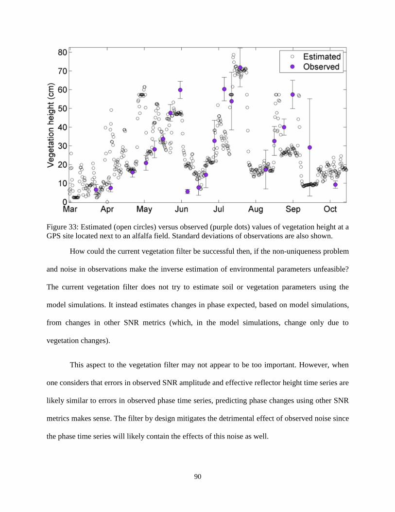
90
Figure 33: Estimated (open circles) versus observed (purple dots) values of vegetation height at a
GPS site located next to an alfalfa field. Standard deviations of observations are also shown.
How could the current vegetation filter be successful then, if the non-uniqueness problem
and noise in observations make the inverse estimation of environmental parameters unfeasible?
The current vegetation filter does not try to estimate soil or vegetation parameters using the
model simulations. It instead estimates changes in phase expected, based on model simulations,
from changes in other SNR metrics (which, in the model simulations, change only due to
vegetation changes).
This aspect to the vegetation filter may not appear to be too important. However, when
one considers that errors in observed SNR amplitude and effective reflector height time series are
likely similar to errors in observed phase time series, predicting phase changes using other SNR
metrics makes sense. The filter by design mitigates the detrimental effect of observed noise since
the phase time series will likely contain the effects of this noise as well.

91
5.5.2 The use of a more complex characteristic SNR equation
It was discussed in Chapters 4 and 5 that oftentimes the presence of vegetation introduces
complexities into SNR interferograms that are not adequately characterized using the metrics
derived from (2). The presence of multiple frequencies in the interferogram or no clear distinct
frequency introduces errors into our estimation of phase and amplitude. The vegetation filter’s
success hinges on the assumption that the errors in phase and amplitude estimation of both
observed and simulated interferograms are the same.
This then, begs the question: Why use Eq. 2 to characterize the interferograms at all?
Why not come up with an alternative characterization of SNR data, one that allows for multiple
frequencies or the variation of amplitude with elevation angle?
Here enter the problems that arise when applying a model to a large network of antennas
and receivers that were not designed to do remote sensing. It has been a struggle to balance
investigating the science behind what drives changes in SNR interferograms, and actually putting
the conclusions of these investigations into practice. Observed SNR data are, for a lack of a
better word, quirky.
To illustrate potential complications that would arise from introducing a more complex
version of (2), let’s assume for a moment that it was possible to introduce variations of amplitude
with elevation into the soil-vegetation model, such that A in (2) was replaced with 𝐴sin (𝐸), which
is the variation of amplitude with elevation angle. This collection of terms that comprise 𝐴sin (𝐸)
all vary to different degrees with changes in soil moisture, vegetation, surface roughness,
topography, tilting of the ground surface and the gain pattern of the antenna, not to mention the

92
phase of the interferogram (which determines ‘where’ in elevation angle the peaks and troughs of
the interferogram begin).
Soil moisture and vegetation changes would be included in 𝐴sin (𝐸) as some sort of
function of the reflection coefficients at that elevation angle, which cannot be determined
analytically due to the nature of variable vegetation canopy heights, among other factors. Figure
34 shows the complicated relationships between elevation angle, the reflection coefficients, and
soil and vegetation parameters. In Figure 34a,b reflection coefficients are presented as a function
of elevation angle for a bare soil, for the case when soil moisture is 0.04 cm3 cm
-3 and also when
soil moisture is 0.4 cm3 cm
-3. One could see that perhaps an analytical relationship could be
derived for the relationship between the uniform soil moisture profile and reflection coefficients
at every elevation angle for the bare soil case. But now, when we introduce a vegetation layer on
top of the soil layer, as in Figure 34c,d, we see that deriving such relationships are not going to
be so simple. (For reference, the vegetation layer added in Figure 34c,d was a 30 cm tall canopy,
with a wet weight of 1 kg m-2
, dry weight of 0.5 kg m-2
, and true density of 500 kg m-3
.)

93
Figure 34: (a) Left- (black) and right-handed (blue) reflection coefficients at circular polarization
for a bare soil with moisture content 0.04 cm3 cm
-3. (b) Same as (a), except moisture content is
0.04 cm3 cm
-3. (c) Same as (a), except now a vegetation layer of 30 cm and permittivity (real
part) of 1.05. (d) Same as (c), except with a soil moisture content of 0.40 cm3 cm
-3.
5.6 Limitations of the vegetation filter
There are several limitations of the vegetation filter that are important to mention. One of
the most obvious limitations is the fact that the filter was designed assuming the base soil
moisture content is 0.15 cm3 cm
-3. Figure 35 shows how the assumed relationships between
Anorm, ALSPnorm, and Δϕ change when the assumed underlying soil moisture content is changed
from 0.05 cm3 cm
-3 to 0.45 cm
3 cm
-3. Even though short term variations in observed SNR
metrics are smoothed out before the vegetation filter is used, if the mean observed soil moisture
content is not 0.15 cm3 cm
-3, there will be error introduced in the estimated phase change due to
vegetation. These errors appear to increase as the SNR amplitude metrics decrease. In order to

94
mitigate these errors, for sites with minimal changes in vegetation, soil moisture content is
allowed to vary randomly in the model simulations. Otherwise, I have found that the vegetation
filter consistently will over-correct for vegetation.
Figure 35: (a) Variation of SNR amplitude metrics with phase for the simulations used in
vegetation filter, assuming an underlying SMC of 0.05 cm3 cm
-3. (b) Variation of SNR amplitude
metrics with phase for the simulations used in vegetation filter, assuming an underlying SMC of
0.45 cm3 cm
-3.
A second important limitation of the filter is that it currently assumes that the a priori
reflector height is known perfectly, and that at some point during the year the site is completely
bare.
The success of the vegetation filter hinges on the assumption that the mischaracterization
of the SNR interferogram using the constant frequency equation is exactly the same in model
simulations and observations. It was mentioned in both [62] and [43] that shifting the dominant
frequency of the interferogram too far away from the bare soil frequency will lead to an overall
mischaracterization of the SNR interferogram and essentially make the phase and amplitude
estimates ‘meaningless’ in that they are no longer representative of the interferogram. The
vegetation filter assumes that modeled SNR metrics and observed metrics are meaningless in the

95
same way and that the meaningless metrics are related to one another in the same way. The filter
thus, to some extent, is matching modeled and observed errors to one another. If and when this
assumption breaks down, the vegetation filter will not work.
In addition, it cannot be stressed enough how important the gain and phase patterns of the
antenna are in determining the characteristics of the SNR interferogram. The relationships
described in this document are very specific to the choke ring antenna. The procedure for
determining the relationships would be the same for other antennas, however, and the soil-
vegetation model still works for other antenna power patterns. It just produces different SNR
interferograms, and hence different SNR metrics.
For example, let us pretend that we have a GPS antenna that is isotropic in both right- and
left-handed circular polarizations. An isotropic antenna allows radiation in from all elevation
angles indiscriminately. This means that the antenna does not suppress ground-reflections from
higher elevation angles. Changes in the amplitude of the SNR interferogram with elevation angle
are now only the result of soil and vegetation parameters. For this experiment, the gain pattern of
the antenna at all elevation angles, for both right- and left-handed polarizations, was set to be the
mean value of the right-handed gain pattern. Other values were tested, and while the absolute
magnitude of the SNR interferogram changed, its variation with elevation angle was the same no
matter the value of gain used.
SNR interferograms for a bare soil and varying moisture content were simulated for the
isotropic antenna. Some examples are shown in Figure 36a. Ignoring the absolute magnitude of
power on the y-axis, Figure 36a shows that there are still oscillations with elevation angle, as
expected, since this is mostly a geometric effect. It also shows that drier soils have a larger
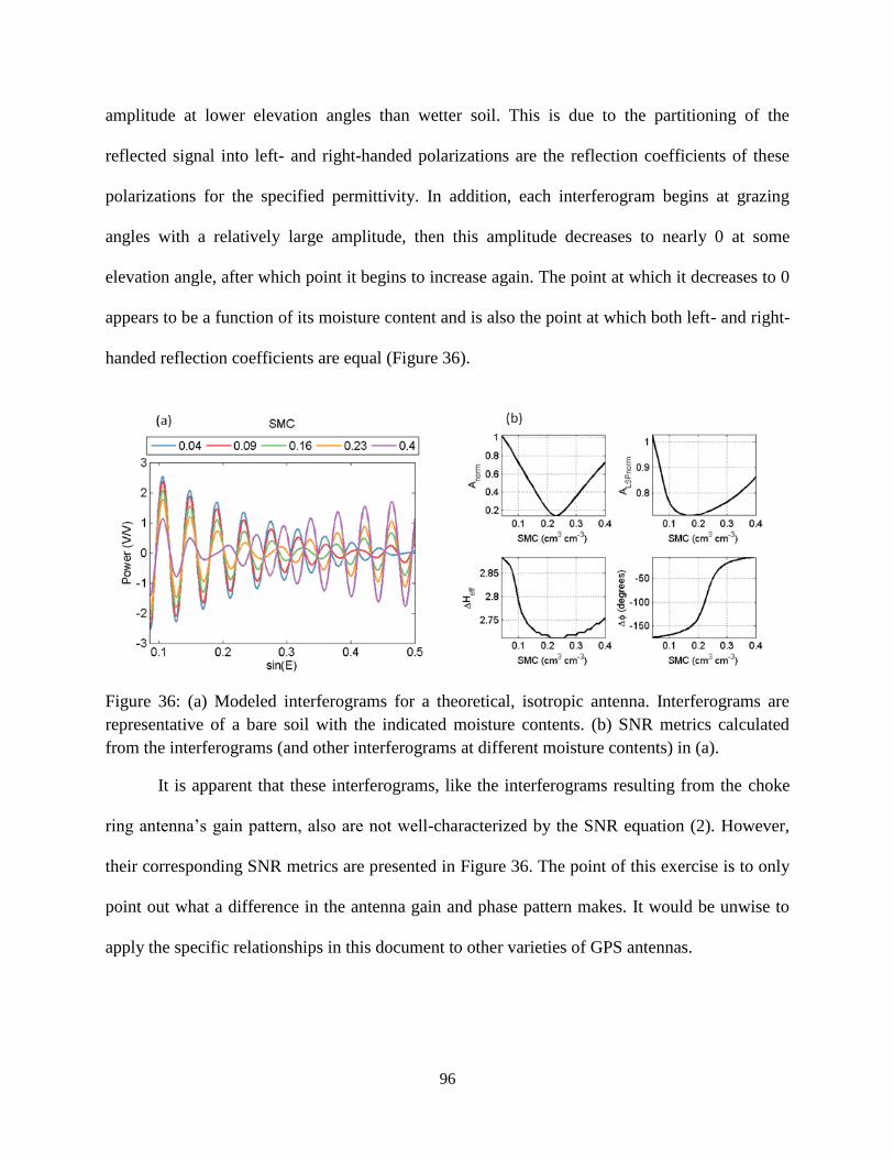
96
amplitude at lower elevation angles than wetter soil. This is due to the partitioning of the
reflected signal into left- and right-handed polarizations are the reflection coefficients of these
polarizations for the specified permittivity. In addition, each interferogram begins at grazing
angles with a relatively large amplitude, then this amplitude decreases to nearly 0 at some
elevation angle, after which point it begins to increase again. The point at which it decreases to 0
appears to be a function of its moisture content and is also the point at which both left- and right-
handed reflection coefficients are equal (Figure 36).
Figure 36: (a) Modeled interferograms for a theoretical, isotropic antenna. Interferograms are
representative of a bare soil with the indicated moisture contents. (b) SNR metrics calculated
from the interferograms (and other interferograms at different moisture contents) in (a).
It is apparent that these interferograms, like the interferograms resulting from the choke
ring antenna’s gain pattern, also are not well-characterized by the SNR equation (2). However,
their corresponding SNR metrics are presented in Figure 36. The point of this exercise is to only
point out what a difference in the antenna gain and phase pattern makes. It would be unwise to
apply the specific relationships in this document to other varieties of GPS antennas.

97
Chapter 6: Soil Moisture Estimations using GPS-IR
This chapter is a departure from the model simulations presented in Chapter 4, though it
does make use of the vegetation filter presented in Chapter 5. This chapter describes how SNR
data are transformed into soil moisture estimations. First, examples of issues that may be present
in empirical data are shown, after which the algorithm currently used for soil moisture estimation
is described.
6.1 Empirical data issues
The vegetation filter cannot resolve all data issues that arise in every observed SNR time
series. Other complications may arise, either due to permanent changes in the environment
(trenching, etc.) or problems within the antenna or receiver that can cause data from one or more
satellite tracks to be of poor quality. These long-term or permanent changes in data quality are
different from the occasional random noise in the interferogram that may cause the data to be of
bad quality for a day or two. Systemic, long-term, or permanent changes to the SNR data quality
for a satellite track have the potential to introduce large errors in soil moisture estimations,
especially for sites with few good satellite tracks to begin with. Here, I will provide examples of
some of these problems and my attempts to mitigate them. However, the problems described
here are by no means the only problems that may be present in the data, though they are some of
the biggest complicating factors in using the vegetation filter on empirical data.
6.1.1 Persistent amplitude anomalies
One example of a persistent amplitude anomaly comes from the GPS sites in Oklahoma
(okl3). PRN 7 Q 4 at okl3 began to exhibit an SNR anomaly on DOY 300 in 2012 (Figure 37).
From 7-12 degrees, amplitude remains depressed throughout the winter, while the amplitude of
surrounding angles increases, as expected. This anomaly persists in the interferograms for this
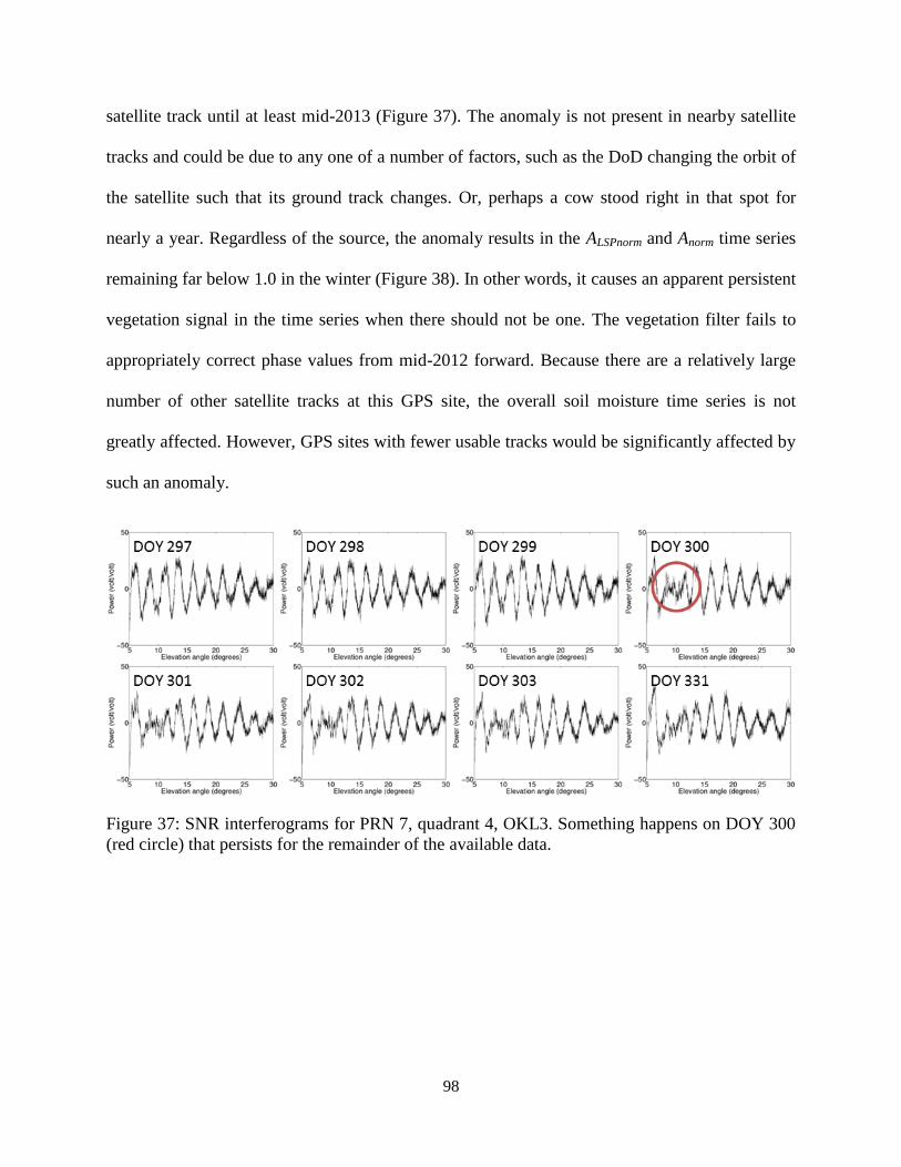
98
satellite track until at least mid-2013 (Figure 37). The anomaly is not present in nearby satellite
tracks and could be due to any one of a number of factors, such as the DoD changing the orbit of
the satellite such that its ground track changes. Or, perhaps a cow stood right in that spot for
nearly a year. Regardless of the source, the anomaly results in the ALSPnorm and Anorm time series
remaining far below 1.0 in the winter (Figure 38). In other words, it causes an apparent persistent
vegetation signal in the time series when there should not be one. The vegetation filter fails to
appropriately correct phase values from mid-2012 forward. Because there are a relatively large
number of other satellite tracks at this GPS site, the overall soil moisture time series is not
greatly affected. However, GPS sites with fewer usable tracks would be significantly affected by
such an anomaly.
Figure 37: SNR interferograms for PRN 7, quadrant 4, OKL3. Something happens on DOY 300
(red circle) that persists for the remainder of the available data.
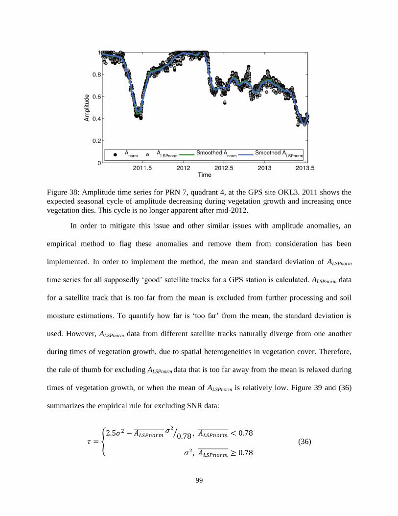
99
Figure 38: Amplitude time series for PRN 7, quadrant 4, at the GPS site OKL3. 2011 shows the
expected seasonal cycle of amplitude decreasing during vegetation growth and increasing once
vegetation dies. This cycle is no longer apparent after mid-2012.
In order to mitigate this issue and other similar issues with amplitude anomalies, an
empirical method to flag these anomalies and remove them from consideration has been
implemented. In order to implement the method, the mean and standard deviation of ALSPnorm
time series for all supposedly ‘good’ satellite tracks for a GPS station is calculated. ALSPnorm data
for a satellite track that is too far from the mean is excluded from further processing and soil
moisture estimations. To quantify how far is ‘too far’ from the mean, the standard deviation is
used. However, ALSPnorm data from different satellite tracks naturally diverge from one another
during times of vegetation growth, due to spatial heterogeneities in vegetation cover. Therefore,
the rule of thumb for excluding ALSPnorm data that is too far away from the mean is relaxed during
times of vegetation growth, or when the mean of ALSPnorm is relatively low. Figure 39 and (36)
summarizes the empirical rule for excluding SNR data:
𝜏 = {2.5𝜎2 − 𝐴𝐿𝑆𝑃𝑛𝑜𝑟𝑚
𝜎2
0.78⁄ , 𝐴𝐿𝑆𝑃𝑛𝑜𝑟𝑚 < 0.78
𝜎2, 𝐴𝐿𝑆𝑃𝑛𝑜𝑟𝑚 ≥ 0.78
(36)

100
Where: 𝜎2 is the standard deviation of the ALSPnorm time series for all good satellite tracks,
𝐴𝐿𝑆𝑃𝑛𝑜𝑟𝑚 is the mean of the ALSPnorm time series for all good satellite tracks, and 𝜏 is the upper
and lower allowance for the deviation of one satellite track’s ALSPnorm time series away from the
mean. Data are excluded when ALSPnorm for a satellite track exceed this limit.
Figure 39: The relationship between ALSPnorm for a single satellite track and the standard
deviation of the mean ALSPnorm time series used to determine how much a particular ALSPnorm time
series is allowed to deviate from the mean.
An example of these bounds for the GPS station in Oklahoma (OKL3) is shown in Figure
40. The empirical filter would not consider much of the aberrant data for PRN 7 quadrant 4 in
2012, indicated by the data (green dots) falling outside the bounds (black lines). It also excludes
data for other satellite tracks at different points in the time series.

101
Figure 40: Time series of ALSPnorm for all supposedly good satellite tracks at OKL3 (colored
dots). Black lines indicate the range of values allowed to be considered for further processing in
the vegetation filter and in soil moisture estimations. Colored points outside this range would be
removed from final soil moisture estimations.
6.1.2 Reflector height considerations
6.1.2.1 Anomalous reflector height shifts
We have at least one example of a potential long-term reflector height change unrelated
to soil moisture or vegetation. At p041 in late 2013, we observe an apparent step change in
reflector height that appears thus far to be permanent. We believe the step change was caused by
the large flooding event in September of that year, with enough sediment being redistributed to
cause changes in the reflector height that should be used as the a priori height.
Figure 41 shows a time series of ΔHeff for PRN 1, quadrant 1. Positive values indicate
that the reflector height is lower than the prescribed a priori height, and vice versa. After the

102
flood, reflector height showed a step change of approximately 3 cm, which would indicate
sedimentation of no more than 3 cm in the footprint of that satellite track (this is the upper bound
because an increase in soil moisture will also cause a decrease in apparent reflector height).
Figure 41: Time series of ΔHeff for PRN 1, quadrant 1 at p041. Circled are time periods of
significant reflector height change. Note the step change in reflector height in late 2013,
coincident with the date of a significant flooding event.
In situ probe data does show that 5 cm average soil moisture did remain quite high post-
flood and into the winter (Figure 42). However, using the same a priori reflector height after the
flood results in soil moisture estimates that are too high. The cyan points in Figure 42 are GPS
estimated soil moisture (with no vegetation filter), and the blue line shows data from TDR
probes. GPS soil moisture tracks nicely with TDR estimates until the flood, after which time they
are too high. If these problems are not detected, errors can obviously be significant.

103
Figure 42: Time series of satellite-track averaged soil moisture estimated (grey points) and in situ
probe data (blue line) for p041 near Marshall, Colorado.
The reflector height problem could manifest itself in ways other than step changes. In the
reflector height time series above, note the time period circled in 2012 with a question mark.
Here, reflector height increases with respect to the a priori height, in other words making the
ground surface appear lower than it actually is. This could be due to changes in the vegetation
canopy, though the reflector height anomaly does not appear to be seasonal in nature, as it
persists into the spring of the following year, which might be an indicator that this wouldn’t be
due to ‘normal’ vegetation effects.
The effect of this anomaly of the phase and subsequently estimated soil moisture time
series is not small. Figure 43 shows the estimated time series along with TDR estimates (here,
theta probe surveys are shown in yellow). The second half of 2012 shows great agreement with
TDR estimates. However, the first half of 2012 shows that GPS estimates are much too high.
This is not due to errors in the relationship between phase and soil moisture, since we see that the
rest of 2012 is fine. Instead, I believe these errors are due to the unexplained reflector height
anomalies described and shown above, as they are well-correlated in time.

104
Figure 43: Data from p041 in Marshall, Colorado. In situ probe data are shown by the blue line.
Yellow points are theta probe data. Grey points are the track-averaged soil moisture estimates
from GPS.
6.1.2.2 Correcting reflector height issues
I have attempted to quantify effects in the phase time series and subsequent soil moisture
estimations due to anomalous variations in reflector height that the vegetation filter might not
account for. Let us create a cosine wave with a known frequency, amplitude, and phase, which
are constant with elevation angle. Frequency is determined using the equation for SNR frequency
as a function of antenna height (4𝜋𝐻
𝜆). For now, let us say that H = 2.4 m, amplitude = 20
volt/volt, and phase = 0 degrees. What if we were to estimate phase and amplitude for this sine
wave, except we are mistaken in the frequency that we use in least-squares? There will be some
amount of error in phase and amplitude estimation. These errors would be similar to expected
errors introduced when the frequency of an observed SNR interferogram change anomalously. In
Figure 44 I show errors in phase and amplitude estimation as a function of the error in frequency
used for least-squares (black line).
This correction is not exactly the same as it would be for re-calculating phase and
amplitude using the raw SNR data. If one were to re-calculate phase using the raw SNR data, the
relationships change. They change because SNR data are not constant frequency, constant
amplitude, or constant phase sine waves. One would expect for these relationships to also depend
on the permittivity of the reflecting surface. Figure 44 (colored points) shows these relationships

105
for bare soil with a uniform moisture profile. Figure 44a shows that, when one uses an a priori
height that is greater than the actual antenna height, the calculated phase will be greater than it
would be if one used the actual antenna height for phase calculation (points to the right of (0,0)
in Figure 44a). The theoretical relationship for these variables, if the SNR data were constant
frequency, amplitude, and phase is shown by the black line. The fact that the black line is quite
close to the SNR data points indicates that phase is relatively constant with elevation angle.
Figure 44: (a) The relationship between mistakes in the a priori reflector height (H0guess) and the
actual antenna height (H0) and corresponding differences in phase. Points are colored by soil
moisture content. The relationship using a constant frequency, amplitude, and phase sine wave is
shown by the black line. (b) The relationship between mistakes in the a priori reflector height
(H0guess) and the actual antenna height (H0) and corresponding differences in amplitude. Points
are colored by soil moisture content. The relationship using a constant frequency, amplitude, and
phase sine wave is shown by the black line. Black points are locations of the maximum values of
amplitude. These locations correspond to peak frequencies in the LSP.
Figure 44b shows the same relationships for amplitude. Phase error does not depend on
the starting value of phase, though amplitude error does, which is why the y-axis in the
amplitude figure above is normalized. Here, amplitude is being normalized with respect to its
‘correct’ value. In this figure, the black, theoretical relationship is no longer close to the
relationship using SNR data. This makes sense, since the SNR data are not constant amplitude.
The locations of maximum amplitudes are indicated by the black points. These locations
106
correspond to the peak frequencies of the LSPs, which also makes sense, as the best estimate of
amplitude will occur when a best-matching frequency is used in its estimation.
I have applied a correction to the phase and amplitude data, using the modeled SNR
relationships in Figure 44. This involves a few assumptions. These relationships vary with soil
moisture, so a median soil moisture content of 0.15 cm3 cm
-3 is assumed. It is also assumed that
the overall correction needed is:
𝐻𝑐𝑜𝑟𝑟𝑒𝑐𝑡𝑖𝑜𝑛 = 𝐻0𝑔𝑢𝑒𝑠𝑠 − 𝐻0
𝐻0 ≅ 𝐻𝑒𝑓��
Where 𝐻𝑐𝑜𝑟𝑟𝑒𝑐𝑡𝑖𝑜𝑛 is the bias needed to be introduced to the SNR metric time series,
𝐻0𝑔𝑢𝑒𝑠𝑠 is the current approximation of the a priori reflector height, and 𝐻0 is the actual a priori
reflector height. 𝐻0 is approximated by the median reflector height in the time series (𝐻𝑒𝑓��).
The equations for the correction, assuming a median SMC of 0.15 cm3 cm
-3 are:
𝐴𝑐𝑜𝑟𝑟𝑒𝑐𝑡𝑒𝑑 =𝐴𝑔𝑢𝑒𝑠𝑠
−18𝐻𝑐𝑜𝑟𝑟𝑒𝑐𝑡𝑖𝑜𝑛2 −2.1𝐻𝑐𝑜𝑟𝑟𝑒𝑐𝑡𝑖𝑜𝑛+1
(37)
𝜙𝑐𝑜𝑟𝑟𝑒𝑐𝑡𝑒𝑑 = 𝜙𝑔𝑢𝑒𝑠𝑠 − 759𝐻𝑐𝑜𝑟𝑟𝑒𝑐𝑡𝑖𝑜𝑛 (38)
𝐻𝑒𝑓𝑓 = 𝐻𝑒𝑓𝑓 − 𝐻𝑐𝑜𝑟𝑟𝑒𝑐𝑡𝑖𝑜𝑛 (39)
Where 𝜙𝑔𝑢𝑒𝑠𝑠 and 𝐴𝑔𝑢𝑒𝑠𝑠 are the phase and amplitude time series currently calculated
using 𝐻0𝑔𝑢𝑒𝑠𝑠, respectively, and 𝜙𝑐𝑜𝑟𝑟𝑒𝑐𝑡𝑒𝑑 and 𝐴𝑐𝑜𝑟𝑟𝑒𝑐𝑡𝑒𝑑 are the corrected time series.
107
Note that in Eq. (38), a 1 cm reflector height drift would equate to a 7.59 degree phase
change. Since the total expected response of phase due to maximum changes in soil moisture is
less than 30 degrees, a 1 cm reflector height drift is actually quite significant.
Let’s revisit our reflector height and phase time series from p041 that were shown in
Figure 41 and Figure 43. In the winter of 2012, reflector height was lower than the a priori
height, which in that plot are positive values on the y-axis (i.e. the reflector height might have
been 1.9 m, and the a priori height was 1.95 m or similar). During the summer of 2012, reflector
height then increases and remains slightly above the a priori height until 2013 (i.e. reflector
height might have been 1.96 m, if the a priori height was 1.95 m). So, in the winter of 2012 at
p041, reflector height variations would be associated with positive values on the x-axis in the
phase error plot in Figure 44. This means that we would expect to see higher than normal phase
estimates during the winter of 2012 at p041. Indeed, in the phase time series (Figure 43), we see
exactly this. Note that this example does not preclude vegetation being the source of this
anomaly, though since it is either not seasonal in nature or just not obviously-seasonal, it could
be from another source.
What happens if the phase and amplitude error relationships (Eq. (37) and (38)) for
constant frequency sinewaves are used on observed SNR data? Let’s examine p041 2012 data
again. Figure 45a shows a reflector height time series for satellite 7, quadrant 3, and the best fit
linear slope to the data. Nearly all satellite tracks in 2012 at p041 have a negative slope, similar
to the one shown below. The reflector height trend can be converted to expected phase changes,
using Eq. (38). These expected changes can be removed from the phase time series, which is
what is shown in Figure 45b. In this figure, black points are the raw phase data, and the red
points are the remainder after the reflector height trend has been removed. Note that there is still

108
a decrease in phase around 2012.4, which does correspond to the expected decrease due to
vegetation growth. There is also an increase in phase at the end of summer, which would be
expected once the vegetation water content decreases.
Figure 45: (a) ΔHeff time series for PRN 7 Q 3 at p041 (black dots) along with the best fit linear
trend to the data (red line). (b) Phase time series for the same satellite track as in (a) (black dots).
Red dots are the phase time series after the linear trend in reflector height has been removed,
using the relationship in Eq. (38).
What is the final effect on the soil moisture time series, if these linear trends are removed
on a track by track basis, and then vegetation filtered as normal? The results are shown in Figure
46. Figure 46a shows the track-averaged time series if there is no linear trend removed, and
Figure 46b shows the time series if these trends are removed. If there is no trend removed,
estimated soil moisture in the winter of 2012 is much too high. Estimated SMC is too low around
2012.7-2012.8. If a linear trend is removed, estimated SMC agrees quite well with in situ probe
SMC in early 2012 and the SMC from 2012.7-2012.8 is also improved, though SMC at the end
of the year is a little too high.
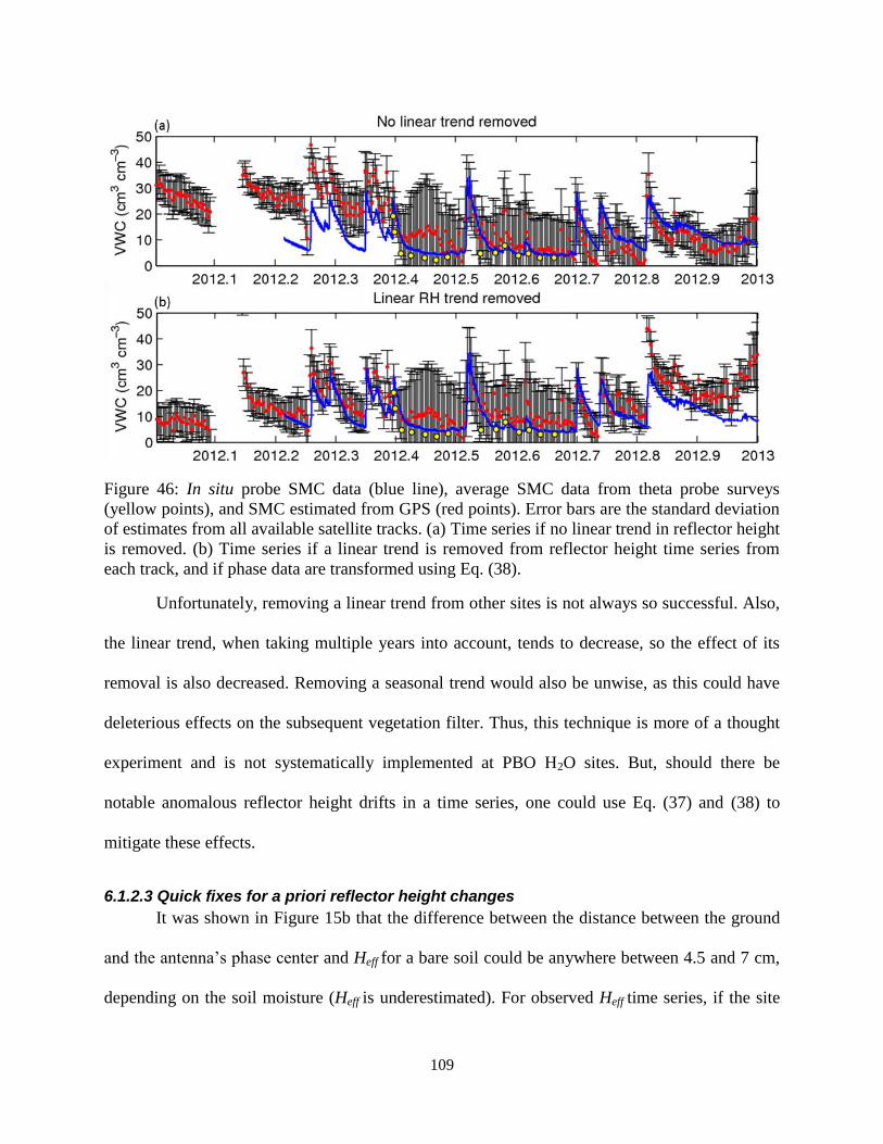
109
Figure 46: In situ probe SMC data (blue line), average SMC data from theta probe surveys
(yellow points), and SMC estimated from GPS (red points). Error bars are the standard deviation
of estimates from all available satellite tracks. (a) Time series if no linear trend in reflector height
is removed. (b) Time series if a linear trend is removed from reflector height time series from
each track, and if phase data are transformed using Eq. (38).
Unfortunately, removing a linear trend from other sites is not always so successful. Also,
the linear trend, when taking multiple years into account, tends to decrease, so the effect of its
removal is also decreased. Removing a seasonal trend would also be unwise, as this could have
deleterious effects on the subsequent vegetation filter. Thus, this technique is more of a thought
experiment and is not systematically implemented at PBO H2O sites. But, should there be
notable anomalous reflector height drifts in a time series, one could use Eq. (37) and (38) to
mitigate these effects.
6.1.2.3 Quick fixes for a priori reflector height changes
It was shown in Figure 15b that the difference between the distance between the ground
and the antenna’s phase center and Heff for a bare soil could be anywhere between 4.5 and 7 cm,
depending on the soil moisture (Heff is underestimated). For observed Heff time series, if the site
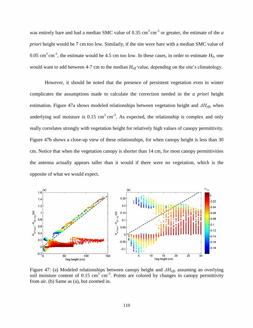
110
was entirely bare and had a median SMC value of 0.35 cm3
cm-3
or greater, the estimate of the a
priori height would be 7 cm too low. Similarly, if the site were bare with a median SMC value of
0.05 cm3
cm-3
, the estimate would be 4.5 cm too low. In these cases, in order to estimate H0, one
would want to add between 4-7 cm to the median Heff value, depending on the site’s climatology.
However, it should be noted that the presence of persistent vegetation even in winter
complicates the assumptions made to calculate the correction needed in the a priori height
estimation. Figure 47a shows modeled relationships between vegetation height and ΔHeff, when
underlying soil moisture is 0.15 cm3
cm-3
. As expected, the relationship is complex and only
really correlates strongly with vegetation height for relatively high values of canopy permittivity.
Figure 47b shows a close-up view of these relationships, for when canopy height is less than 30
cm. Notice that when the vegetation canopy is shorter than 14 cm, for most canopy permittivities
the antenna actually appears taller than it would if there were no vegetation, which is the
opposite of what we would expect.
Figure 47: (a) Modeled relationships between canopy height and ΔHeff, assuming an overlying
soil moisture content of 0.15 cm3 cm
-3. Points are colored by changes in canopy permittivity
from air. (b) Same as (a), but zoomed in.

111
Residual vegetation could, then, negate the need for the adjustment of the estimated a
priori reflector height. However, in the absence of detailed site information, it’s difficult to
determine what the residual vegetation state is. After all, if the minimal vegetation canopy is
greater than 14 cm tall, then the adjustment of the a priori reflector height would need to be even
larger than for just bare soil. Corrections are generalizations and may not work everywhere.
One could apply a correction to all time series, such that the a priori reflector height
value is ‘essentially’ the median of the complete Heff time series. I write ‘essentially’ because
recalculating phase and amplitude for nearly all satellite tracks at every site would be too time-
consuming. Most satellite tracks have been assigned H0 values quite close to the median value,
though in some cases, values are a few centimeters off (Figure 48). This is because the a priori
height is set once, but over time, the median value of the reflector height time series may change.
Instead of recalculating phase and amplitude using the raw SNR data and the median value of
H0, one could use Eq. (37) and (38) as a sort of ‘quick fix.’ I do not necessarily advocate for this
approach, but it can give a first look at what happens when the value of H0 is changed.
6.1.2.4 Effect of changing the a priori reflector height
The theoretical relationship between phase and soil moisture is based on the assumption
that phase is calculated using the true value of H0, though observed phase data are calculated
using the median value of Heff, or close to it (Figure 48). Therefore, it would be natural to think
that if the ‘true value’ of H0 were somehow found, the RMSE between GPS-derived soil
moisture and in situ data would decrease. Here, I show a few examples to see whether or not this
is the case. I compare the RMSE between GPS soil moisture and in situ data on a track-by-track
basis, first using the phase time series calculated using the current a priori reflector height, and

112
then re-calculating phase after introducing a reflector height bias. Phase is recalculated using Eq.
(38).
Figure 48: Examples of the set a priori reflector height (H0) versus the median reflector height,
colored by PRN number and quadrant. (a) OKL3 (b) BCGR (c) p041 (d) grs2.
Results are shown in Figure 49. The left column of Figure 49 indicates that there can be a
wide range of RMSE values for each satellite track at a specific site, either exhibiting the failure
of the vegetation filter to remove vegetation for these tracks or perhaps indicating that some
tracks are just not usable. The right column shows the difference in RMSE that one would get
when introducing a bias versus no bias (0 cm). Results from these three sites indicate that

113
introducing additional biases into the a priori reflector height will cause inconsistent increases
and decreases in RMSE across satellite tracks. Some satellite tracks are not sensitive to changes
in the bias, whereas others show large effects. At this point, it appears that the addition of further
reflector height biases will not significantly affect the RMSE of a site as a whole, without
introducing track-specific biases for each track.

114

115
Figure 49: (left column) The RMSE between GPS soil moisture for individual satellite tracks and
in situ probes at three sites, with additional reflector height biases added in. (right column) Same
data as in the left column, but with the RMSE at 0 cm additional bias subtracted out.
6.2 Soil moisture retrieval algorithm
Here is described the algorithm that is currently used to produce the soil moisture
estimations for the PBO H2O network. The vegetation filter from Chapter 5 is included in the
algorithm. Parts of the algorithm are also described more completely in other chapters, though to
make the steps of the algorithm coherent, I have chosen to repeat them in this section so that
jumping around to other chapters isn’t necessary.
1. Selection of useful satellite tracks
Not all satellite tracks at a particular site are useful for GPS-IR. Tracks should have
consistent reflections between satellite elevation angles of 5-25 or 5-30 degrees; oscillations in
the interferogram for higher angles are obscured by the antenna’s gain pattern. Tracks should
also not be obstructed by trees or buildings or reflect from manmade surfaces like roads. A track
should have a relatively stable singular dominant frequency for periods of the year when
vegetation water content or height is nearly constant. In general, the power (ALSP) of the
dominant frequency (Heff) should be at least twice as high as the power of the noise or second
most powerful frequency in the periodogram.
Examples of SNR data from two useful satellite tracks (red and green) and two tracks
with significant noise corruption (blue and orange) are shown in Figure 4c. The noise-corrupted
satellite tracks lack any dominant frequency, which could introduce significant errors in
subsequent phase and amplitude estimation (Figure 4d). Part of the reason for these two tracks
lacking a dominant frequency is due to the fact that the two satellites ground tracks pass over a
region of sloped topography (see Figure 50 for a digital elevation model and ground paths of the
satellite tracks). Satellite tracks that encompass areas with large topographic changes (on the
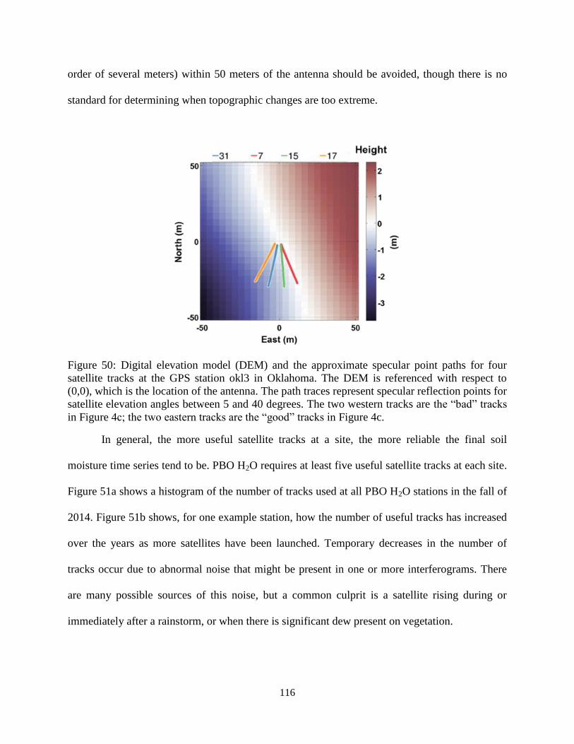
116
order of several meters) within 50 meters of the antenna should be avoided, though there is no
standard for determining when topographic changes are too extreme.
Figure 50: Digital elevation model (DEM) and the approximate specular point paths for four
satellite tracks at the GPS station okl3 in Oklahoma. The DEM is referenced with respect to
(0,0), which is the location of the antenna. The path traces represent specular reflection points for
satellite elevation angles between 5 and 40 degrees. The two western tracks are the “bad” tracks
in Figure 4c; the two eastern tracks are the “good” tracks in Figure 4c.
In general, the more useful satellite tracks at a site, the more reliable the final soil
moisture time series tend to be. PBO H2O requires at least five useful satellite tracks at each site.
Figure 51a shows a histogram of the number of tracks used at all PBO H2O stations in the fall of
2014. Figure 51b shows, for one example station, how the number of useful tracks has increased
over the years as more satellites have been launched. Temporary decreases in the number of
tracks occur due to abnormal noise that might be present in one or more interferograms. There
are many possible sources of this noise, but a common culprit is a satellite rising during or
immediately after a rainstorm, or when there is significant dew present on vegetation.

117
Figure 51: (a) Histogram of the number of satellite tracks used at PBO H2O stations during the
fall of 2014. (b) Time series of the number of tracks used at site p038. Step increases occur when
additional satellites were launched.
2. Estimation of each track’s a priori reflector height, H0
Due to microtopography surrounding the antenna, the a priori reflector height (H0) is not
known perfectly and has to be estimated from the SNR data. PBO H2O uses the median of Heff
data that are free of snow events and significant vegetation for the value of H0 for each satellite
track.
3. Calculate SNR metrics: ϕ, A, Heff, and ALSP
SNR metrics for each day and each satellite track are calculated using the procedure
described in section 2.6.1 and 2.6.2.
4. Quantify vegetation effects
As described in section 5.1, if a satellite track’s Anorm time series stays below 0.78 for an
extended period of time is likely to be affected by something other than soil moisture variations

118
(i.e. vegetation changes). A track whose time series remains above 0.78 may have small
vegetation effects, though for these cases it is difficult to determine whether decreases in Anorm
are from vegetation or from soil moisture changes. In these cases, one may skip to Step 6 in the
algorithm below and not use the vegetation filter.
If the GPS site does have a significant vegetation effect as determined by the Anorm time
series, then one should proceed to the section “Algorithm for removing vegetation effects”
before estimating soil moisture in Step 6. If there is a significant vegetation effect but the effect
is of a short-enough duration, then the phase data when Anorm is below 0.78 may be removed,
without using the vegetation filter. However, simply removing the phase data without
implementing a vegetation correction will result in error for periods surrounding the affected
interval, which are still affected by vegetation growth. It is up to the user whether or not greater
error is acceptable for the tradeoff in simplicity of data analysis.
6. Soil moisture estimation
At GPS sites with limited seasonal change in vegetation, as indicated by the Anorm time
series, soil moisture estimation is relatively straightforward. We use data from the site mfle as an
example.
6a. Zero the phase time series
For each year of data, the phase time series for each satellite track is zeroed, such
that the lowest values are near zero. Sites in the PBO H2O network are zeroed by first
calculating the mean of the lowest 15% of observed phase data for each year and each
track. The mean is then subtracted from the phase time series. 15% is a parameter that
may be decreased or increased, depending on the amount of noise present in the data.

119
Phase time series are zeroed yearly; this assumes that soil moisture at the site
reaches its residual value at some point during the year. This assumption is generally
valid, at least for the PBO H2O sites. Yearly zeroing is done so that any period of
anomalously low phase data (due to non-removal of vegetation effects or random noise)
will not affect the entire time series.
6b. Determine the residual soil moisture content
Because temporal phase changes are relative and the minimum moisture content
of a soil is never zero, the baseline phase value needs to be associated with the soil’s
residual moisture content. Residual moisture content, SMCresid, is correlated with soil
texture, and this data can be found in publicly-available data sets such as the U.S.
Geological Survey’s STATSGO data set [63]. However, optimally the residual moisture
content of the soil at the site would be measured through the use of gravimetry or time
domain reflectometry probes.
6c. Estimate the soil moisture time series for each satellite track
Modeled relationships between phase and soil moisture are used to compute the
estimated soil moisture time series.
𝑆𝑀𝐶𝑡 = 𝑆∆𝜙𝑡 + 𝑆𝑀𝐶𝑟𝑒𝑠𝑖𝑑 (40)
Where S is the expected slope between phase and soil moisture. For time series
with no significant vegetation affect, S = 1.48 cm3 cm
-3 deg
-1.
7. Estimate the soil moisture time series for the GPS site as a whole
To estimate site-averaged soil moisture on the daily timescale, the median soil moisture
value of all tracks for each day is used. Uncertainties are computed as the standard deviation of
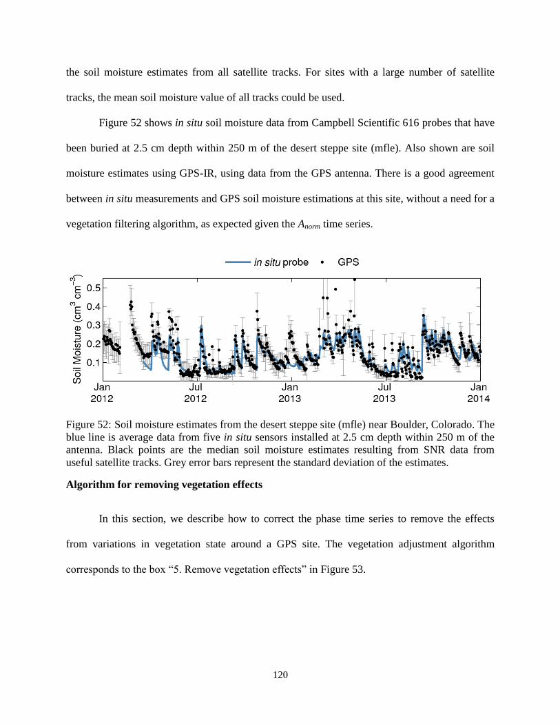
120
the soil moisture estimates from all satellite tracks. For sites with a large number of satellite
tracks, the mean soil moisture value of all tracks could be used.
Figure 52 shows in situ soil moisture data from Campbell Scientific 616 probes that have
been buried at 2.5 cm depth within 250 m of the desert steppe site (mfle). Also shown are soil
moisture estimates using GPS-IR, using data from the GPS antenna. There is a good agreement
between in situ measurements and GPS soil moisture estimations at this site, without a need for a
vegetation filtering algorithm, as expected given the Anorm time series.
Figure 52: Soil moisture estimates from the desert steppe site (mfle) near Boulder, Colorado. The
blue line is average data from five in situ sensors installed at 2.5 cm depth within 250 m of the
antenna. Black points are the median soil moisture estimates resulting from SNR data from
useful satellite tracks. Grey error bars represent the standard deviation of the estimates.
Algorithm for removing vegetation effects
In this section, we describe how to correct the phase time series to remove the effects
from variations in vegetation state around a GPS site. The vegetation adjustment algorithm
corresponds to the box “5. Remove vegetation effects” in Figure 53.

121
Figure 53: Flowchart depicting steps in the algorithm to estimate soil moisture for a GPS site.

122
We use data from the Oklahoma GPS site to demonstrate the importance of adjusting
phase time series for vegetation. Fig. 6 (bottom) shows that the Oklahoma GPS station, okl3, is
surrounded by vegetation that varies in water content and height, both seasonally and from year-
to-year. Figure 54a shows how following the simple soil moisture estimation procedure
described above would lead to poor agreement with in situ data. Because an increase in
vegetation causes a decrease in phase, and the residual moisture content is set to the lowest
observed phase value, vegetation growth causes the resulting soil moisture estimations to be
over-estimated in winter. Clearly, an adjustment for vegetation is needed at this site. This could
be determined solely from the Anorm time series, which shows values as low as 0.5 during the
growing season.
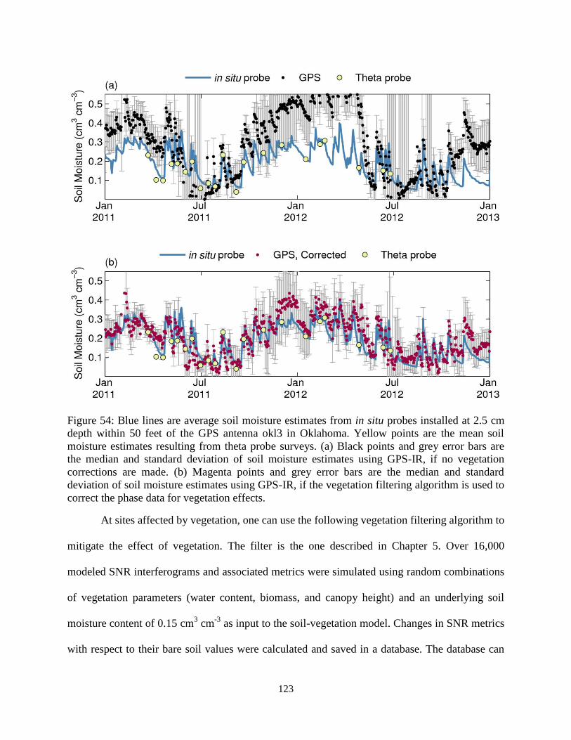
123
Figure 54: Blue lines are average soil moisture estimates from in situ probes installed at 2.5 cm
depth within 50 feet of the GPS antenna okl3 in Oklahoma. Yellow points are the mean soil
moisture estimates resulting from theta probe surveys. (a) Black points and grey error bars are
the median and standard deviation of soil moisture estimates using GPS-IR, if no vegetation
corrections are made. (b) Magenta points and grey error bars are the median and standard
deviation of soil moisture estimates using GPS-IR, if the vegetation filtering algorithm is used to
correct the phase data for vegetation effects.
At sites affected by vegetation, one can use the following vegetation filtering algorithm to
mitigate the effect of vegetation. The filter is the one described in Chapter 5. Over 16,000
modeled SNR interferograms and associated metrics were simulated using random combinations
of vegetation parameters (water content, biomass, and canopy height) and an underlying soil
moisture content of 0.15 cm3 cm
-3 as input to the soil-vegetation model. Changes in SNR metrics
with respect to their bare soil values were calculated and saved in a database. The database can

124
be queried to estimate the change in phase corresponding to any observed combination of Anorm,
ALSPnorm, and ΔHeff time series. The same random combinations of vegetation parameters were
then used with underlying soil moisture contents of both 0.05 cm3 cm
-3 and 0.45 cm
3 cm
-3 and
the soil-vegetation model was run again. Another database was created from these simulations,
which shows how SNR metrics are expected to respond to changes in underlying soil moisture
given a particular vegetation state.
Now we describe how to use the model database to remove vegetation effects from
observed SNR phase data. This is done on a track-by-track basis, as the input data (SNR metrics)
are all track specific.
5a. Process data for use in the vegetation filter
The vegetation filter assumes that the phase time series has been zeroed such that
data most affected by vegetation go below zero. In order to conform to this convention,
the phase time series should be zeroed with respect to the median of the highest values in
the time series. We have found the median of the highest 15% of observed phase data
works well.
Use a low-pass filter to remove high frequency noise associated with soil moisture
fluctuations from the Anorm, ALSPnorm, and ΔHeff time series. The ends of the Anorm, ALSPnorm,
and ΔHeff time series are first padded to decrease edge effects. Thirty repetitions of the
mean of the first and last 15 days of Anorm, ALSPnorm, and ΔHeff values are appended to the
beginning and end of each time series.
Anorm, ALSPnorm, and ΔHeff are smoothed using a Savitzky-Golay filter, a least-
squares smoothing method. The S-G filter tends to be more successful than a moving

125
average or moving median filter, since with the right parameters it does not introduce
time lags into smoothed time series and will not smooth out the maximum or minimum
extents of the time series. Most of the time, a moving average filter is sufficient, though
one must be careful to not over-smooth time series that may have significant, though
short-lived, vegetation effects.
5b. Estimate and subtract the phase change from vegetation from the observed time
series
A linear nearest neighbor search algorithm is used to find the estimated phase
caused by vegetation fluctuations, given observed Anorm, ALSPnorm, and ΔHeff and the
modeled database described in Chapter 5. Thus, one can estimate the effects of vegetation
on phase using time series of the other three SNR metrics. No field observations of
vegetation amount are needed. Estimated phase changes from the database are smoothed
through time using the same Savitzky-Golay filter, and the padded ends are removed.
The expected phase changes due to vegetation are subtracted from the observed,
unsmoothed phase time series, resulting in phase time series that indicate soil moisture
variations only.
𝜙𝑆𝑀𝐶,𝑡 = ∆𝜙𝑡 − 𝜙𝑣𝑒𝑔,𝑡 (41)
Where 𝜙𝑆𝑀𝐶,𝑡 is the expected phase change due to soil moisture at time t, ∆𝜙𝑡 is the
original observed time series at time t, and 𝜙𝑣𝑒𝑔is the predicted phase change due to
vegetation at time t. This relationship is a simplification, as it is based on the assumption
that the total phase change is a linear combination of the phase change due to soil
moisture and the phase change due to vegetation.
5c. Determine the sensitivity change between phase and soil moisture due to vegetation

126
Expected sensitivity changes between phase and soil moisture are estimated,
using the same procedure and linear search algorithm described above. The sensitivity of
phase to soil moisture will change depending on the extent of overlying vegetation, and
thus the slope of the relationship between phase and soil moisture, S, will change
throughout the year. Equation 40 used in Step 6 thus does not have a constant value of S
for data processed with the vegetation filter, but rather a value that varies depending upon
the vegetation state.
Once the phase data are processed with the vegetation filter, one can calculate a soil
moisture time series for each track (Step 6, Figure 53). Residual moisture content is selected in
the same way as for a bare soil case (Step 6b). When converting phase to soil moisture, S is a
function of time, as described in Step 5c. The soil moisture time series for a phase time series
filtered for vegetation will thus be a variant of Eq. (40):
𝑆𝑀𝐶𝑡 = 𝑆𝑡∆𝜙𝑆𝑀𝐶,𝑡 + 𝑆𝑀𝐶𝑟𝑒𝑠𝑖𝑑 (42)
As described above, the median of the track soil moisture time series is taken to be
representative of the soil moisture of the site as a whole. There are additional uncertainties due to
assumptions made in the vegetation filtering algorithm, which are not yet incorporated into final
soil moisture estimates.
The vegetation-corrected soil moisture time series for the GPS station in Oklahoma is
shown in Figure 54b, using the median soil moisture value for all tracks. Agreement between the
GPS-derived soil moisture estimations and those from in situ data has been much improved over
the non-vegetation-filtered estimations (Figure 54a). In particular, the large wintertime
deviations described in the previous section have been significantly reduced.

127
6.3 Validation of soil moisture retrievals
This section describes the validation results from using the soil moisture retrieval
algorithm described in 6.2 with observed data. Before results are presented, however, it is
important to note that the choice of in situ data against which to compare GPS soil moisture time
series is not a trivial one. All of the GPS soil moisture estimations presented here are either
compared against the average from Theta probe surveys, or against Campbell Scientific 616
probe data. It is easy to assume that these in situ data represent the ‘true’ value of soil moisture.
However, differences in spatial sensitivities of the probes versus GPS estimates (see Chapter 2.2)
will lead to inherent differences in the data.
In addition, the probes themselves will not yield data that are perfectly comparable to
even other probe data. Figure 55a shows a soil pit dug as part of the SMAP in situ test bed
experiment in Oklahoma. Several different types of soil moisture probes were buried at the same
depths and close to one another, to allow for the comparison of soil moisture time series. Figure
55b shows time series from three different types of probes from one of these pits; each probe was
buried at 5 cm depth. There are clear differences between the probes, and the RMS error between
each kind of probe is on the order of 0.03 cm3 cm
-3. One might question the practically of
producing GPS soil moisture time series, or satellite soil moisture estimations, with an RMS
error below 0.04 cm3 cm
-3 when the probes themselves show such disagreement. Even so, since
we conducted several soil moisture surveys with a theta probe, I will present validation results
plotted against data from the theta probe.

128
Figure 55: (a) A 1 m deep pit in Oklahoma with several types of soil moisture probes. (b) Probe
data from three different brands of probes buried at the same depth, next to one another.
Figure 56a is a scatterplot of soil moisture estimated using GPS-IR and the algorithm
presented in 6.2 and in situ data from theta probe surveys. No bias has been removed from the
data. Not all sites with theta probe surveys are shown; these are just a subset of the data.
Figure 56: GPS soil moisture estimates versus in situ soil moisture data taken with a theta probe.
GPS soil moisture values represent the mean of the soil moisture estimates from available useful
tracks. Theta probe estimates are the mean of at least 25 points measurements taken within 50 m

129
of the GPS antenna during each survey. (a) Estimates using the vegetation filter. (b) Estimates
without using the vegetation filter.
There is good correspondence between the two methods of soil moisture estimation; the
RMS error is 0.053 cm3 cm
-3. This is a bit higher than the 0.04 cm
3 cm
-3 required by the SMAP
mission, though some of these estimations were produced during times when vegetation extent
was relatively high (>1 kg m-2
). For comparison, the GPS-IR soil moisture estimates without
using the vegetation filter are shown in Figure 56b (note the scale difference of the x-axis). The
RMS error for these estimates is 0.12 cm3 cm
-3. Thus, the addition of the vegetation has
decreased the RMS error by almost 0.07 cm3 cm
-3.
One improvement that has not yet been made to the data is taking into account the fact
that the residual moisture content has been set for each satellite track. Therefore, the lowest of
the mean moisture content of the tracks is going to always be somewhat higher than the residual.
This could lower the RMS error for some sites like p032, for example. I also believe that if I
were actually to develop an outlier detection algorithm beyond the bare bones one currently in
place, the RMS error could decrease further.
6.4 Effect of changing model parameters
The soil moisture algorithm outlined in 6.2 has several parameters that are important in
the final soil moisture estimations. Here, I describe the parameters in more detail and the
potential effects of changing some of the key parameters.
Table 7 contains a summary of the parameters that are used in the algorithm. Some of
these parameters, though not all, were mentioned in 6.2. Many of the parameters, such as the
parameters relating to amplitude normalization or phase zeroing, only need to be set
‘reasonably,’ i.e. a small change in the parameter will not visibly affect soil moisture time series.

130
Other parameters, such as the a priori reflector height offset (for some sites) and choice of
smoothing method and associated parameters, are extremely important for the algorithm to work.
I will now show the effects of changing these parameters.
Table 7: Description of parameters used in the soil moisture algorithm.
Parameter Description Abbreviation Range of values Default
value
H0 offset* hbias 0-9 cm 0 cm
Outlier removal remoutli 0 (no) or 1 (yes) 1
Correct for Heff anomalies Acc_rhdrift 0 (no) or 1 (yes) 0
Amplitude veg flag Smm 0-1 0.8
Use all tracks, or the list of good
ones Which_sats 0 (all) or 1 (good tracks) 1**
Fraction of ϕ to zero to zphival 0.05-0.25 0.15
Method to fill in NaN values nanopt 0-5 5
# of days to calculate amplitude
variance for outliers Ampvarday 3-7 3
Amplitude variance limit (V/V)
for outliers ampvarlimit 0-3 1
Remove phase outliers remoutliP 0 (no) or 1 (yes) 1
Zero the entire phase time series
(or yearly) zallts
0 (yearly) or 1 (full time
series) 0
2nd
ϕ zeroing parameter zphivalP 0.05-0.25 0.15
For veg filter, zeroing w.r.t. max
ϕvalues Mzphival 0.05-0.25 0.15
Smoothing method Sm_method 1 (Savitzky-Golay) or 2 1
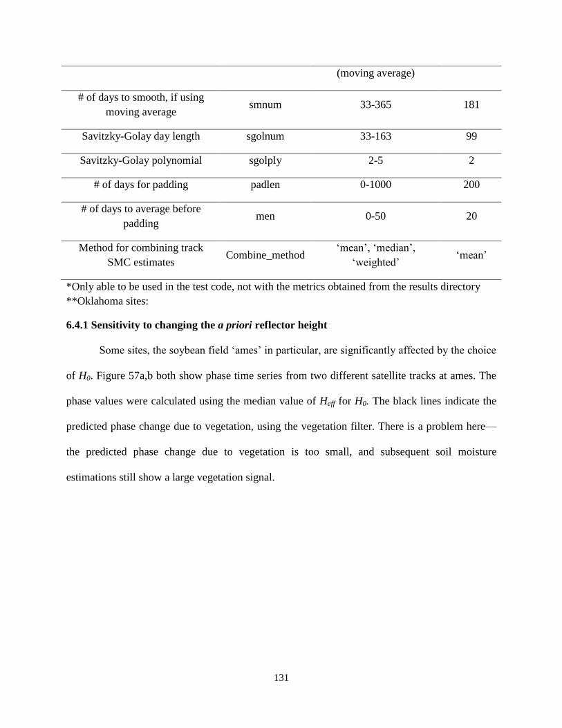
131
(moving average)
# of days to smooth, if using
moving average smnum 33-365 181
Savitzky-Golay day length sgolnum 33-163 99
Savitzky-Golay polynomial sgolply 2-5 2
# of days for padding padlen 0-1000 200
# of days to average before
padding men 0-50 20
Method for combining track
SMC estimates Combine_method
‘mean’, ‘median’,
‘weighted’ ‘mean’
*Only able to be used in the test code, not with the metrics obtained from the results directory
**Oklahoma sites:
6.4.1 Sensitivity to changing the a priori reflector height
Some sites, the soybean field ‘ames’ in particular, are significantly affected by the choice
of H0. Figure 57a,b both show phase time series from two different satellite tracks at ames. The
phase values were calculated using the median value of Heff for H0. The black lines indicate the
predicted phase change due to vegetation, using the vegetation filter. There is a problem here—
the predicted phase change due to vegetation is too small, and subsequent soil moisture
estimations still show a large vegetation signal.
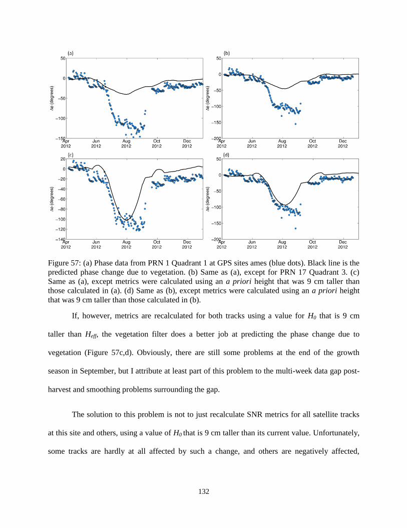
132
Figure 57: (a) Phase data from PRN 1 Quadrant 1 at GPS sites ames (blue dots). Black line is the
predicted phase change due to vegetation. (b) Same as (a), except for PRN 17 Quadrant 3. (c)
Same as (a), except metrics were calculated using an a priori height that was 9 cm taller than
those calculated in (a). (d) Same as (b), except metrics were calculated using an a priori height
that was 9 cm taller than those calculated in (b).
If, however, metrics are recalculated for both tracks using a value for H0 that is 9 cm
taller than Heff, the vegetation filter does a better job at predicting the phase change due to
vegetation (Figure 57c,d). Obviously, there are still some problems at the end of the growth
season in September, but I attribute at least part of this problem to the multi-week data gap post-
harvest and smoothing problems surrounding the gap.
The solution to this problem is not to just recalculate SNR metrics for all satellite tracks
at this site and others, using a value of H0 that is 9 cm taller than its current value. Unfortunately,
some tracks are hardly at all affected by such a change, and others are negatively affected,

133
meaning that adding 9 cm to H0 actually causes an over-prediction of phase change due to
vegetation.
6.4.2 Sensitivity to changes in the smoothing method
This section might be unnecessary if a better alternative for the linear nearest-neighbor
search could be found. Predicted phase changes due to vegetation can be noisy, due to the search
algorithm, the number of simulations used in the search algorithm, and mismatches between
simulations and observations. Because of this noise, it is necessary to smooth the phase change
predictions before removing them from the observed phase time series. And, because of the
noise, the changing the smoothing method or the method’s parameters can change the phase
predictions significantly. Although I will only describe the differences between moving average
and Savitzky-Golay filters, I have also tried other filtering techniques (Fourier filters and
wavelets, for example) and have found similar results to the ones described below.
An example of the different phase predictions for different smoothing methods is shown
in Figure 58. In this figure, the different panels represent either predictions made with the
Savitzky-Golay filter (Figure 58a,c) or the moving average filter (Figure 58b,d). The filters span
either 15 days (Figure 58a,b) or 63 days (Figure 58c,d). It is apparent that the 15-day filters are
characterized by too much high frequency noise. The 63-day filters are less influenced by noise,
though the moving average filter is starting to be over-smoothed, whereas the Savitzky-Golay
filter better preserves the timing and magnitude of phase change due to increases in vegetation.
134
Figure 58: All data in this figure are from PRN 25 Quadrant 2 at GPS station okl3. Blue dots in
each panel are the raw phase observations—data end in July 2013 due to power issues at the site.
Black lines are the predicted phase changes due to vegetation using different smoothing
methods: (a) Savitzky-Golay filter, 15 day span (b) moving average filter, 15 day span (c)
Savitzky-Golay filter, 63 day span (d) moving average filter, 63 day span.

135
Chapter 7: Error Quantification
This chapter focuses on potential sources of error in soil moisture estimates. The errors
mentioned here are only errors that can be quantified using the electrodynamic model. Errors
due to issues like noise in SNR observations, the DoD changing the orbit of a satellite, etc. are
not included.
7.1 Errors for bare soil
7.1.1 Imperfect knowledge of a priori reflector height
The electrodynamic model assumes that the distance from the ground to the phase center
of the antenna, is known perfectly. This is what is deemed the a priori reflector height. However,
even for a bare, flat soil in model simulations, the calculated reflector heights never match the
input H0. Model simulations instead show that, if one were to estimate antenna height using
calculated reflector height, one would underestimate the height of the antenna by 3-7 cm,
depending on the soil moisture. This is due to the fact that the permittivity of the ground is not
high enough to act as a perfect reflector. Changes in microtopography surrounding a real antenna
will add additional uncertainty to this estimate.
The errors introduced from this uncertainty are illustrated in the following example. The
model was run for a bare soil, using a set of soil moisture observations as input. Phase is then
calculated using three different a priori reflector heights: the ‘known’ antenna height, a height
that is 3 cm shorter than the known height, and a height that is 7 cm shorter than the known
height. Phase is then converted into its corresponding soil moisture time series, using the
equation derived from the bare soil model, which assumes H0 is known perfectly. The resulting

136
soil moisture time series along with the synthetic soil moisture input data (in situ) are shown in
Figure 59.
Figure 59: Synthetic soil moisture observations (in situ) and corresponding soil moisture
estimates, assuming different under-estimations of the a priori reflector height (colored points).
We see that, as antenna height is underestimated, there is an underestimation of soil
moisture, particularly for high soil moisture. Although the RMS error for the 7 cm case is only
0.013 cm3 cm
-3, when the target RMS error is below 0.04, errors in antenna height estimation
(for a bare, flat soil with no other sources of errors) will account for 25% of the target RMS
error, which is certainly not insignificant. Conversely, if one were to over-estimate antenna
height, soil moisture would thus be overestimated as well.
In theory, if one had a long enough ‘perfect’ reflector height time series (i.e. perfectly
flat, satellite tracks not moving spatially, no noise in estimations, no vegetation, etc.) one could
probably estimate the correct a priori height perfectly by adding ~3-5 cm (depending on the
soil’s residual SMC value) to the highest reflector height observation.

137
7.1.2 Vertical gradients in SMC profiles
The current retrieval algorithm assumes that soil moisture profiles do not vary with depth,
though in reality gradients will occur—immediately after a rainstorm the surface will be wetter
than at depth and otherwise the surface will nearly always be drier. This was briefly mentioned
in Section 4.3.3.5.
Shows results from model simulations generated from 1500 soil moisture profiles for a
loam soil with an a priori height of 2.4 m. Soil moisture was specified at 2.5, 7.5, and 20 cm
depth, which were random values between 0.05 and 0.40. The model interpolates between depths
to get the full soil moisture profile, the number of layers being 1001, which means each
interpolated layer was 0.2 mm thick. Because of the cubic extrapolation method to find soil
moisture at the surface, some surficial soil moisture values were nearly 0, which is unrealistic, so
these simulations were removed. This resulted in about 1000 total simulations from which the
Each soil moisture profile has an associated phase value from the SNR data. Figure 60a
shows phase versus the surface soil moisture value and phase versus the average soil moisture
value for the top 5 cm of soil.

138
Figure 60: (a) Phase versus soil moisture for ~1000 randomly-generated soil moisture profiles.
Points are plotted by either the value of the soil moisture at the surface (black), or by the value of
the average soil moisture of the top 5 cm of soil (red). (b) The same model simulations used in
(a) are plotted by the difference between the surface soil moisture and the average top 5 cm soil
moisture (red points). Points to the right of zero are wetter on the surface than at depth, and vice
versa.
We see that soil moisture at depths beneath the surface do not change the retrieval
algorithm between surface soil moisture and phase (black points all cluster closely around the
constant soil moisture profile relationship). It is also apparent that if there is a strong soil
moisture gradient in the near-surface profile (i.e. surface SMC is not close the average SMC for
the top 5 cm of soil), the correlations between probe estimates and GPS estimates could disagree
significantly.
In the example below we will consider the soil moisture gradient to just be the difference
between the soil moisture at the surface and the average value over the top 5 cm. A negative
value indicates that the soil is wetter at depth, and vice versa. I will use the quadratic retrieval
algorithm (fit a quadratic to modeled, non-varying SMC profiles, i.e. Figure 12b) to see errors in
surface soil moisture estimation for the above simulations, as a function of the soil moisture
gradient. We will also see what the perceived errors could be if we compare the soil moisture
estimates to the actual average soil moisture in the top 5 cm. In this case, we are quantifying the

139
disagreement we could see when we compare our soil moisture estimations to probe data. Of
course this experiment assumes that both wetting and drying profiles are nearly equally present
in real field data, even though drying profiles will likely occur more frequently for the vast
majority of sites.
The results are in Figure 60b. If one uses the retrieval algorithm derived from Figure 12b
on the phase data from the simulated soil moisture profiles, and compares the estimated soil
moisture to the actual surface soil moisture, then one would get errors similar to the black dots in
Figure 60b. Errors are not large, except for the case of extreme soil moisture gradients. However,
if you compare the estimated soil moisture to the actual average soil moisture over the top 5 cm
of soil, errors are much larger (red dots). Thus, extreme wetting or drying profiles could result in
large disagreement between in situ probes and GPS estimations.
7.1.3 Differences in antenna height
The relationship between soil moisture and phase does not significantly change if you
have a short (1 m) vs. tall (3 m) antenna Figure 61. The ‘baseline’ phase value does change,
however, but since the phase time series is always zeroed, this does not affect soil moisture
estimations.
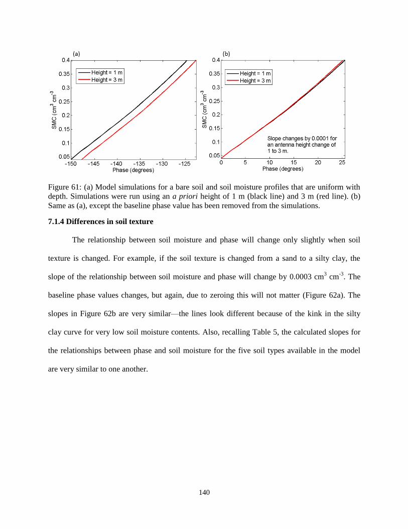
140
Figure 61: (a) Model simulations for a bare soil and soil moisture profiles that are uniform with
depth. Simulations were run using an a priori height of 1 m (black line) and 3 m (red line). (b)
Same as (a), except the baseline phase value has been removed from the simulations.
7.1.4 Differences in soil texture
The relationship between soil moisture and phase will change only slightly when soil
texture is changed. For example, if the soil texture is changed from a sand to a silty clay, the
slope of the relationship between soil moisture and phase will change by 0.0003 cm3 cm
-3. The
baseline phase values changes, but again, due to zeroing this will not matter (Figure 62a). The
slopes in Figure 62b are very similar—the lines look different because of the kink in the silty
clay curve for very low soil moisture contents. Also, recalling Table 5, the calculated slopes for
the relationships between phase and soil moisture for the five soil types available in the model
are very similar to one another.

141
Figure 62: (a) The relationship between phase and soil moisture for uniform moisture profiles,
specifying the soil texture as either a sand (black line) or silty clay (red line). (b) Same as (a),
except with the baseline phase values removed.
7.1.5 Changes in soil temperature
A few of the PBO H2O sites are located in areas with large diurnal or seasonal
temperature swings, such as those in Alaska or in deserts like the Sevilleta. Therefore, it is
important to know how changes in ground temperature will affect SNR metrics. In order to
investigate this, I used published relationships between soil temperature, soil texture, and
permittivity found in [64]. One shortcoming of these data was that soil moisture was kept at 0.30
cm3 cm
-3, so different moisture contents could respond differently to changes in temperature.
Data from [64] were used in the electrodynamic model, assuming a bare soil, constant
temperature profile with depth, and constant soil moisture with depth of 0.30 cm3 cm
-3. The
ground temperature was varied, SNR data were simulated, and both phase and amplitude were
computed. As always, the elevation angle range for the SNR data was the standard 5-30 degrees.
Results from this experiment are shown in Figure 63. It appears that changes in soil temperature
only minimally affect SNR metrics, except during periods of thawing or freezing, during which
effects will be significant.

142
Figure 63: (top) Effect of ground temperature changes on phase, when SMC = 0.3 cm3 cm
-3.
(bottom) Effect of ground temperature changes on amplitude, when SMC = 0.3 cm3 cm
-3.
7.1.6 Changes in receiver temperature
I do not have a way to model receiver temperature. Though, there does appear to be a
correlation between average surface temperature and amplitude at grs2 in New Mexico (Figure
64a), but not as much of a correlation between surface temperature and phase (Figure 64b).
Amplitude and temperature appear to perhaps be inversely correlated, which I believe would be
expected. Since there isn’t a corresponding effect in phase, I think the amplitude effect is indeed
due to temperature and not to temperature/soil moisture or temperature/vegetation correlations. If
the temperature effect is real, this could affect how successful the vegetation filter is (an increase
in temperature could be mistaken for an increase in vegetation).

143
Figure 64: (a) Observed relationship between the daily-average surface temperature and
amplitude for several satellite tracks (colored points) at site grs2 in New Mexico. (b) Same as (a),
except for phase.
7.1.7 Surface roughness
The soil moisture retrieval algorithm is based on the assumption that the surface
surrounding the antenna is perfectly flat—of course, this is never really the case. It is expected
that increasing surface roughness will increase the amount of signal scattering and decrease the
reflection coefficient. The rough surface reflection coefficient is given by [65]:
𝑆𝑟 = exp (−2 (2𝜋ℎ𝑟𝑚𝑠 sin 𝐸
𝜆)
2
) (43)
Where hrms is the root mean square surface height irregularity. Sr may be multiplied by the
horizontal or vertical reflection coefficients to obtain the total reflection coefficient at either
horizontal or vertical polarizations. These reflection coefficients may then be transformed into
reflection coefficients for circular polarization via the equations in 4.1.1.
I have not included any divergence factor, which takes into account a curved earth, into
the reflection coefficient calculations. However, I expect the divergence factor to be negligible,

144
since it is related to the ratio of (basically) the specular reflection point distance to the antenna
and the radius of the Earth, and this value is nearly zero [65].
I added surface roughness into the bare soil model and simulated SNR interferograms for
varying soil moisture (uniform with depth) and surface roughness. Figure 65 shows how the
relationships between SNR metrics and soil moisture are expected to change with increasing
surface roughness. As surface roughness increases, the range of the response of metrics to soil
moisture decreases (i.e. sensitivity decreases). Effective reflector height does not change
significantly for roughness increases up to 10 cm. Surface roughness affects the absolute
maximum value of amplitude, though when normalized, the effect of surface roughness is greatly
diminished. Surface roughness perhaps most significantly affects phase, though only after the
roughness value is larger than about 4 cm.
Since surface roughness changes the slope between phase and soil moisture, using the
modeled slope for a flat surface will introduce errors into soil moisture estimations. The
theoretical error in soil moisture estimations that would be introduced from the presence of
surface roughness is shown in Figure 66. If one wants the error to be less than 0.04 cm3 cm
-3,
then the surface roughness must not exceed ~6 cm.

145
Figure 65: The effect of surface roughness on phase, amplitude, and effective reflector height.
Lines are colored by the surface roughness height. Soil moisture profiles were uniform with
depth.

146
Figure 66: The RMS error (in cm3 cm
-3) between simulated soil moisture and ‘truth’ if no
correction for surface roughness is made in the slope between phase and soil moisture. The
dashed line denotes the 0.04 cm3 cm
-3 target for this project.
7.2 Errors for vegetated environments
Here, I address errors or uncertainties in the vegetation filter described in Chapter 5,
which takes into account changes in amplitude, LSP amplitude, and reflector height in order to
estimate changes in phase from vegetation.
7.2.1 Imperfect knowledge of antenna height
Just like in the bare soil case, we still do not have a perfect knowledge of antenna height
for areas with soil and vegetation. Unfortunately vegetation in natural environments causes
additional uncertainty in knowing what the a priori reflector height should be. Natural
environments are almost never completely devoid of vegetation; even in the winter there will be
some amount of standing vegetation. Thus, the a priori reflector height that is estimated for these

147
environments is the height for bare soil plus some amount of residual vegetation. Figure 47
showed how the estimated a priori height could be higher or lower than the actual antenna
height, depending on vegetation amount.
This is important because the modeled relationships between SNR metrics to correct for
vegetation are not linear. In Section 4.4.2 and Figure 25, it was determined that vegetation water
content affects both phase and amplitude linearly until water content exceeds 1-1.5 kg m-2
. (This
is true for vegetation types that have a 1:1 relationship with true density and water content; it’s
not quite as linear for those that do not.) However, the relationship between metrics and other
metrics is not as straightforward, given the wide scatter in relationships in Figure 31. Therefore,
if we attempt to use any vegetation filter that assumes relationships between ALSPnorm and Anorm
for example, there will be errors due to this residual vegetation amount. Vegetation filters,
without extensive knowledge of vegetation at the site, assume that at some point during the year,
vegetation extent was zero and that the a priori height was determined from this time period.
This could be the case for agricultural environments, but not for natural areas.
We can quantify theoretical errors in the vegetation filter from using an incorrect a priori
reflector height to estimate phase and amplitude. Let us take a random set of 365 of the model
simulations used in the vegetation filter (out of ~16000 possible simulations) and recalculate
phase and amplitude, using an a priori height that is X cm away from the actual antenna height.
This subset becomes our one year dataset of synthetic observations. Here, we still assume that
we know the ‘bare soil’ amplitude and phase values, though in reality these are also unknown.
We can implement the vegetation filter on our synthetic observations and see how uncertainties
vary with errors in the a priori height. Figure 67 shows how errors in phase change estimation
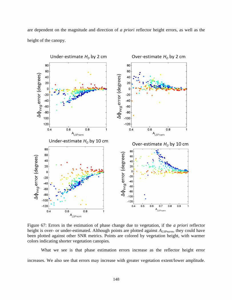
148
are dependent on the magnitude and direction of a priori reflector height errors, as well as the
height of the canopy.
Figure 67: Errors in the estimation of phase change due to vegetation, if the a priori reflector
height is over- or under-estimated. Although points are plotted against ALSPnorm, they could have
been plotted against other SNR metrics. Points are colored by vegetation height, with warmer
colors indicating shorter vegetation canopies.
What we see is that phase estimation errors increase as the reflector height error
increases. We also see that errors may increase with greater vegetation extent/lower amplitude.

149
An over-estimation of antenna height would subsequently lead to an ‘overfixing’ of phase, and
vice versa. Recall that normally, the a priori height will be under-estimated, leading to an
‘underfixing’ of phase with the vegetation filter. This could potentially be the cause of the
significant differences in predicted phase at ames when the a priori height is changed, as in
Figure 57.
The relationships in Figure 67 may change with the presence of residual vegetation, as
shown in the reflector height plot in the beginning of this section. General rules of thumb for
estimating these errors, however, is difficult, since we do not know what our reflector height
error is, or any information as to canopy height or permittivity.

150
Chapter 8: Future Work
There are many ways that the soil moisture retrieval algorithm could be improved in the
future to make the addition of new sites easier and to refine retrievals at existing sites.
8.1 Improvements in model simulations for the vegetation filter
As was stated previously, the current plane-stratified model does not take into account the
effects of plant geometry on the reflected signal, nor does it consider volume scattering. I have
found that the vegetation filter does not work well for agricultural environments such as bcgr
(alfalfa field) or ames (soybean field). I believe part of the problem lies in the plane stratified
approach to modeling the vegetation canopy. It is possible that including these effects could
provide insight into why relationships between SNR metrics are not well simulated at these sites.
In addition, modeling sites with topography or a significant slope and the effects of the slope on
SNR metric relationships would probably improve retrievals, though doing so could reduce the
algorithm’s efficiency.
The vegetation filter could also be refined to improve retrievals. The filter is currently
comprised of thousands of random combinations of vegetation parameters, which is useful when
there is no a priori vegetation information for a site. However, in reality, we do know at least a
little bit about most of the sites in the PBO network. For example, we know that nearly all of the
sites in Montana are natural grasslands, and we have dozens of in situ vegetation measurements
from some of these stations. It could be advantageous, for the sites in Montana, to restrict the
vegetation parameter sets in the filter to only those representing typical grasslands. Similarly,
one could restrict the filter for desert environments, and so on.

151
In addition, the assumption in the simulations that soil moisture does not change
seasonally, concurrently with vegetation, is a limitation that needs further work. The current
simulations used in the filter assume the bare soil moisture content is 0.15 cm3 cm
-3 and allows
soil moisture and vegetation amount to change concurrently. If the simulations instead assume
the bare soil moisture content is 0.25 cm3 cm
-3 and that soil moisture when vegetation is present
decreases to 0.15 cm3 cm
-3, then the filter predicts different changes in vegetation.
Figure 68a shows, for one satellite track at site p042, the phase observations and the
predicted phase change due to vegetation. We see that phase is under-predicted around 2013.75.
Figure 68b shows how the predictions change if the simulations are changed to those described
above (0.25 cm3 cm
-3 decreasing to 0.15 cm
3 cm
-3). Phase is no longer under-predicted.
Figure 68: (a) Observed phase data from PRN 25 Quadrant 4 at site p042 in Wyoming (open
circles) and predicted phase change due to vegetation (black line), using the model simulations
assuming an underlying soil moisture of 0.15 cm3 cm
-3. (b) Same as (a) except the model

152
simulations assumed a bare soil moisture content of 0.25 cm3 cm
-3 that decreases to 0.15 cm
3
cm−3
when vegetation is present.
Similarly, Figure 69a shows soil moisture retrievals for site masw in California, using the
standard vegetation filter. Soil moisture is unrealistically high in the winters of 2012 and 2013.
However, if the alternate simulations are used in the vegetation filter, soil moisture retrievals are
more realistic (Figure 69b). More work needs to be done to determine whether imposing
different soil moisture restrictions in the model simulations would improve retrievals across
sites, and if so, what the optimum restrictions are.
Figure 69: GPS-estimated soil moisture for site masw in California. (a) The vegetation filter used
model simulations that assumed an underlying soil moisture content of 0.15 cm3 cm
-3. (b) The
vegetation filter used model simulations that assumed the bare soil moisture content was 0.25
cm3 cm
-3and decreased to 0.15 cm
3 cm
-3when vegetation was present.

153
An effort should also be made to better incorporate the uncertainties described in Chapter
8 into the soil moisture retrievals. Currently, the error bars represent the variability in retrievals
from different satellite tracks. If this variability could be decreased, either by better outlier
identification or by improving the algorithm, then the errors described in Chapter 8 could be
more reasonably incorporated.
8.2 Improvements in quality control of observations
Even if the vegetation filter were refined, a big challenge that still remains is better
identifying when and where data from tracks are reliable. Although one method of identifying
bad data based on amplitude was described in Section 6.1.1, there are other issues that must be
mitigated, such as satellite maneuvers that change the ground track (and a priori reflector
height). One could recognize that the DoD changed the satellite’s orbit slightly and adjust the
track’s a priori height accordingly, though automating this and other quality controls is
desirable.
The saying, “One bad apple can spoil the bunch,” definitely applies to final soil moisture
estimations, especially if and when the mean of the track-by-track soil moisture estimates is
taken. It is expected that there is some variation in the track-by-track soil moisture estimations,
though occasionally one track will perform much worse than the others. Reasons for worse
performance can be related to the empirical issues described above, but there are also times when
the vegetation filter does not do a good job. Here, I will describe what some of these outliers may
look like, and how I have attempted to remove them.
Figure 70 shows what the track-by-track soil moisture estimates look like at site okl3,
along with in situ data. The light orange points in this figure are data from PRN 25 Quadrant 1,
and we see that right before mid-2011, the soil moisture estimates are unreasonably high for a

154
very short period. Similarly, the light blue points in this figure are data from PRN 1 Quadrant 2,
which also show unreasonably high soil moisture retrievals in the first half of 2012.
Although retrievals from both satellite tracks are anomalously high, their reasons for
being so are different. PRN 25 (orange points) are too high because for an unknown reason the
amplitude time series began to decrease before the phase time series did, which caused phase to
be ‘over-fixed’ during that brief interval. PRN 1 (blue dots), on the other hand was not corrected
enough in 2012 for vegetation. This is possibly because the smoothing algorithm over-smoothed
the reflector height time series, making the magnitude of vegetation change appear smaller than
it actually was. The end result is anomalously high soil moisture during the spring months.
Improving the smoothing algorithm could mitigate this issue. However, there is not
currently a way to automatically detect when there are outliers, since there are many causes for
outliers, as was just described.

155
Figure 70: Time series of track-by-track estimated soil moisture (colored dots are retrievals from
different PRNs), and in situ data (black line) from Oklahoma GPS site okl3.

156
Chapter 9: Conclusions
Here I have described the development of an algorithm to retrieve soil moisture from
GPS ground reflection data, which includes corrections for deleterious effects from vegetation
growth. The algorithm was designed for use with the choke ring antennas frequently used in GPS
networks, though similar algorithms with different parameters could be developed for use with
different types of antennas.
Initial observations of SNR metrics from several GPS sites indicated a change in soil
moisture induced changes in SNR metrics to different degrees. Observations also indicated that
seasonal changes in SNR metrics were associated with vegetation growth and senescence. Due to
spatial heterogeneities in soil moisture and vegetation and other unknowns (receiver influences
on the ground-reflected signal, etc.) an electrodynamic model was used to elucidate the effects of
soil moisture and vegetation changes alone on the ground-reflected signal.
The electrodynamic model was originally developed for a bare, planar surface. How
changes in soil moisture affected each SNR metric was first investigated for this simple case. It
was found that the SNR metric phase is the variable most indicative of changes in soil moisture,
though all SNR metrics are affected by soil moisture change. Soil texture and antenna height
were determined to not significantly impact the relationships between soil moisture and SNR
metrics. Additionally, it was also determined that surface soil moisture change was the most
important driver of SNR metric change, as opposed to changes in soil moisture at depth.
The allowance for a vegetation canopy was next included in the model, and this model
was validated against observations from four different GPS sites. It was determined that the
height of the canopy as well as its permittivity, which itself is a combination of other vegetation

157
parameters, are the two metrics that determine how SNR metrics respond to changes within in
the canopy. Commonly measured vegetation parameters, such as vegetation water content, will
only be well correlated with SNR metric change if it is also correlated with other vegetation
canopy parameters, in particular the true density of vegetation. All SNR metrics were determined
to be affected by vegetation growth. It is nearly impossible to untangle the influences of
concurrent changes in soil moisture and vegetation, for short or low permittivity canopies.
Vegetation growth mimics a decrease in soil moisture; a rise in soil moisture mimics a decrease
in vegetation growth.
In order to remove the effect of vegetation on the phase time series, which is then used to
estimate changes in soil moisture, a vegetation filter was designed. The vegetation filter used
SNR metrics from model simulations that represented how theoretical vegetation canopies would
affect SNR metrics. The filter does not estimate vegetation; rather, it compares three of the four
observed SNR metrics to modeled metrics and predicts how much phase, the fourth metric, likely
changed due to changes in the vegetation canopy.
The vegetation filter makes up part of the final soil moisture algorithm. Possible errors in
final soil moisture estimates are caused by inaccurate values of the a priori reflector height,
confounding influences of underlying soil moisture on total SNR metric change that is not well
represented in the model simulations, and inadequate smoothing of the SNR metric time series.
Validation of the algorithm and vegetation filter at sites with in situ soil moisture data
indicates that the addition of the vegetation filter improves retrieval accuracy. Data resulting
from the algorithm are available for download at http://xenon.colorado.edu/portal.

158
Bibliography
[1] D. Entekhabi, I. Rodriguez-Iturbe, and F. Castelli, “Mutual interaction of soil moisture state and
atmospheric processes,” J. Hydrol., vol. 184, pp. 3–17, 1996.
[2] A. Robock, K. Y. Vinnikov, G. Srinivasan, J. K. Entin, S. E. Hollinger, N. A. Speranskaya, S. Liu,
and A. Namkhai, “The Global Soil Moisture Data Bank,” Bull. Am. Meteorol. Soc., vol. 81, no. 6,
pp. 1281–1299, 2000.
[3] R. D. Koster, P. a Dirmeyer, Z. Guo, G. Bonan, E. Chan, P. Cox, C. T. Gordon, S. Kanae, E.
Kowalczyk, D. Lawrence, P. Liu, C.-H. Lu, S. Malyshev, B. McAvaney, K. Mitchell, D. Mocko,
T. Oki, K. Oleson, A. Pitman, Y. C. Sud, C. M. Taylor, D. Verseghy, R. Vasic, Y. Xue, and T.
Yamada, “Regions of strong coupling between soil moisture and precipitation.,” Science (80-. ).,
vol. 305, no. 5687, pp. 1138–40, Aug. 2004.
[4] K. Rajkai and B. E. Ryden, “Measuring areal soil moisture distribution with the TDR method,”
Geoderma, vol. 52, pp. 73–85, 1992.
[5] B. D. Entekhabi, E. G. Njoku, P. E. O. Neill, K. H. Kellogg, W. T. Crow, W. N. Edelstein, J. K.
Entin, S. D. Goodman, T. J. Jackson, J. Johnson, J. Kimball, J. R. Piepmeier, R. D. Koster, N.
Martin, K. C. Mcdonald, M. Moghaddam, S. Moran, R. Reichle, J. C. Shi, M. W. Spencer, S. W.
Thurman, L. Tsang, and J. Van Zyl, “The soil moisture active passive (SMAP) mission,” Proc.
IEEE, vol. 98, no. 5, pp. 704–716, 2010.
[6] J. R. Wang, E. T. Engman, J. C. Shiue, and M. Rusek, “Observations of Microwave Dependence
on Soil Moisture , Surface Roughness , and Vegetation Covers,” IEEE Trans. Geosci. Remote
Sens., vol. GE-24, no. 4, pp. 510–516, 1986.
[7] F. T. Ulaby, R. K. Moore, and A. K. Fung, Microwave Remote Sensing Active and Passive-
Volume II: Radar Remote Sensing and Surface Scattering and Enission Theory. Addison-Wesley
Publishing Company, 1982.
[8] L. Tsang, J. A. Kong, and R. T. Shin, Theory of microwave remote sensing, 1st ed. Wiley-
Interscience, 1985.
[9] M. T. Hallikainen, F. T. Ulaby, M. C. Dobson, M. A. El-Rayes, and L.-K. Wu, “Microwave
Dielectric Behavior of Wet Soil-Part 1: Empirical Models and Experimental Observations,” IEEE
Trans. Geosci. Remote Sens., vol. GE-23, no. 1, pp. 25–34, 1985.
[10] I. M. Fuks and A. G. Voronovich, “Wave diffraction by rough interfaces in an arbitrary plane-
layered medium,” Waves in Random Media, vol. 10, pp. 37–41, 2000.
[11] W. J. Rawls, D. L. Brakensiek, and K. E. Saxton, “Estimation of Soil Water Properties,” Trans.
ASAE, vol. 25, no. 5, pp. 1316–1320, 1982.

159
[12] P. A. Ferre, D. L. Rudolph, and R. G. Kachanoski, “Spatial Averaging of Water Content by Time
Domain Reflectometry: Implications for Twin Rod Probes with and without Dielectric Coatings,”
Water, vol. 32, no. 2, pp. 271–279, 1996.
[13] F. T. Ulaby, P. P. Batlivala, and M. C. Dobson, “Microwave Backscatter Dependence on Surface
Roughness , Soil Moisture , and Soil Texture : Part 1I-Bare Soil,” IEEE Trans. Geosci. Electron.,
vol. GE-16, no. 4, pp. 286–295, 1978.
[14] E. G. Njoku and D. Entekhabi, “Passive microwave remote sensing of soil moisture,” J. Hydrol.,
vol. 184, no. 1–2, pp. 101–129, Oct. 1996.
[15] M. Schwank, C. Mätzler, S. Member, M. Guglielmetti, and H. Flühler, “L-Band Radiometer
Measurements of Soil Water Under Growing Clover Grass,” IEEE Trans. Geosci. Remote Sens.,
vol. 43, no. 10, pp. 2225–2237, 2005.
[16] T. J. Jackson and D. E. Le Vine, “Mapping surface soil moisture using an aircraft-based passive
microwave instrument: algorithm and example,” J. Hydrol., vol. 184, pp. 85–99, 1996.
[17] I. Mladenova, V. Lakshmi, T. J. Jackson, J. P. Walker, O. Merlin, and R. A. M. de Jeu,
“Validation of AMSR-E soil moisture using L-band airborne radiometer data from National
Airborne Field Experiment 2006,” Remote Sens. Environ., vol. 115, no. 8, pp. 2096–2103, Aug.
2011.
[18] T. J. Jackson, D. M. Le Vine, C. T. Swifi, T. J. Schmugge, and F. R. Schiebe, “Large Area
Mapping of Soil Moisture Using the ESTAR Passive Microwave Radiometer in Washita ’ 92,”
Remote Sens. Environ., vol. 53, pp. 27–37, 1995.
[19] F. T. Ulaby, P. C. Dubois, and J. van Zyl, “Radar mapping of surface soil moisture,” J. Hydrol.,
vol. 184, pp. 57–84, 1996.
[20] A. W. Western, G. Bloschl, and R. B. Grayson, “Geostatistical characterisation of soil moisture
patterns in the Tarrawarra catchment,” J. Hydrol., vol. 205, pp. 20–37, 1998.
[21] A. Gomez-Plaza, M. Martinez-Mena, J. Albaladejo, and V. M. Castillo, “Factors regulating spatial
distribution of soil water content in small semiarid catchments,” J. Hydrol., vol. 253, pp. 211–226,
2001.
[22] G. Baroni, B. Ortuani, a. Facchi, and C. Gandolfi, “The role of vegetation and soil properties on
the spatio-temporal variability of the surface soil moisture in a maize-cropped field,” J. Hydrol.,
vol. 489, pp. 148–159, May 2013.
[23] L. Brocca, R. Morbidelli, F. Melone, and T. Moramarco, “Soil moisture spatial variability in
experimental areas of central Italy,” J. Hydrol., vol. 333, no. 2–4, pp. 356–373, Feb. 2007.
[24] J. S. Famiglietti, J. W. Rudnicki, and M. Rodell, “Variability in surface moisture content along a
hillslope transect: Rattlesnake Hill, Texas,” J. Hydrol., vol. 210, no. 1–4, pp. 259–281, Sep. 1998.

160
[25] C. D. Hall and R. A. Cordey, “Multistatic Scatterometry,” in Proceedings of IGARSS ’88
Symposium, 1988, pp. 561–562.
[26] V. U. Zavorotny and A. G. Voronovich, “Scattering of GPS Signals from the Ocean with Wind
Remote Sensing Application,” IEEE Trans. Geosci. Remote Sens., vol. 38, no. 2, pp. 951–964,
2000.
[27] A. Komjathy, V. U. Zavorotny, P. Axelrad, G. H. Born, and J. L. Garrison, “GPS Signal Scattering
from Sea Surface : Wind Speed Retrieval Using Experimental Data and Theoretical Model,”
Remote Sens. Environ., vol. 73, pp. 162–174, 2000.
[28] E. Cardellach, G. Ruffini, D. Pino, A. Rius, A. Komjathy, and J. L. Garrison, “Mediterranean
Balloon Experiment: ocean wind speed sensing from the stratosphere, using GPS reflections,”
Remote Sens. Environ., vol. 88, no. 3, pp. 351–362, Dec. 2003.
[29] S. T. Lowe, C. Zuffada, Y. Chao, P. Kroger, L. E. Young, and J. L. Labrecque, “5-cm-Precision
aircraft ocean altimetry using GPS reflections,” Geophys. Res. Lett., vol. 29, no. 10, pp. 10–13,
2002.
[30] M. Martin-Neira, “A passive reflectometry and interferometry system (PARIS): Application to
ocean altimetry,” ESA J., vol. 17, pp. 331–355, 1993.
[31] A. Komjathy, J. Maslanik, V. U. Zavorotny, P. Axelrad, and S. J. Katzberg, “Sea Ice Remote
Sensing Using Surface Reflected GPS Signals,” in Geoscience and Remote Sensing Symposium,
2000., 2000, pp. 2855–2857.
[32] M. D. Jacobson, “Inferring Snow Water Equivalent for a Snow-Covered Ground Reflector Using
GPS Multipath Signals,” Remote Sens., vol. 2, no. 10, pp. 2426–2441, Oct. 2010.
[33] E. Cardellach, F. Fabra, A. Rius, S. Pettinato, and S. D’Addio, “Characterization of dry-snow sub-
structure using GNSS reflected signals,” Remote Sens. Environ., vol. 124, pp. 122–134, Sep. 2012.
[34] N. Rodriguez-Alvarez, A. Aguasca, E. Valencia, X. Bosch-Lluis, I. Ramos-Perez, H. Park, A.
Camps, and M. Vall-llossera, “Snow monitoring using GNSS-R techniques,” Geosci. Remote
Sens. Symp., pp. 4375–4378, 2011.
[35] D. S. Masters, “Surface Remote Sensing Applications of GNSS Bistatic Radar : Soil Moisture and
Aircraft Altimetry,” University of Colorado at Boulder, 2004.
[36] N. Rodriguez-Alvarez, X. Bosch-lluis, A. Camps, I. Ramos-Perez, E. Valencia, H. Park, and M.
Vall-llossera, “Vegetation Water Content Estimation Using GNSS Measurements,” IEEE Geosci.
Remote Sens. Lett., vol. 9, no. 2, pp. 282–286, 2012.
[37] N. Rodriguez-Alvarez, X. Bosch-Lluis, A. Camps, A. Aguasca, M. Vall-llossera, E. Valencia, I.
Ramos-Perez, and H. Park, “Review of crop growth and soil moisture monitoring from a ground-
based instrument implementing the Interference Pattern GNSS-R Technique,” Radio Sci., vol. 46,
no. 6, p. n/a–n/a, Dec. 2011.

161
[38] P. Ferrazzoli, L. Guerriero, N. Pierdicca, and R. Rahmoune, “Forest biomass monitoring with
GNSS-R: Theoretical simulations,” Adv. Sp. Res., vol. 47, no. 10, pp. 1823–1832, May 2011.
[39] K. M. Larson and F. G. Nievinski, “GPS snow sensing: results from the EarthScope Plate
Boundary Observatory,” GPS Solut., vol. 17, no. 1, pp. 41–52, Mar. 2013.
[40] F. G. Nievinski and K. M. Larson, “Forward modeling of GPS multipath for near-surface
reflectometry and positioning applications,” GPS Solut., vol. 18, no. 2, pp. 309–322, Jun. 2014.
[41] E. E. Small, K. M. Larson, and J. J. Braun, “Sensing vegetation growth with reflected GPS
signals,” Geophys. Res. Lett., vol. 37, no. 12, pp. 1–5, Jun. 2010.
[42] S. G. Evans, E. E. Small, and K. M. Larson, “Comparison of vegetation phenology in the western
USA determined from reflected GPS microwave signals and NDVI,” Int. J. Remote Sens., vol. 35,
no. 9, pp. 2996–3017, Apr. 2014.
[43] W. Wan, K. M. Larson, E. E. Small, C. C. Chew, and J. J. Braun, “Using geodetic GPS receivers
to measure vegetation water content,” GPS Solut., May 2014.
[44] K. M. Larson, J. J. Braun, E. E. Small, V. U. Zavorotny, E. D. Gutmann, and A. L. Bilich, “GPS
Multipath and Its Relation to Near-Surface Soil Moisture Content,” IEEE J. Sel. Top. Appl. Earth
Obs. Remote Sens., vol. 3, no. 1, pp. 91–99, 2010.
[45] K. M. Larson, E. E. Small, E. Gutmann, A. Bilich, P. Axelrad, and J. Braun, “Using GPS
multipath to measure soil moisture fluctuations: initial results,” GPS Solut., vol. 12, no. 3, pp.
173–177, Aug. 2008.
[46] F. G. Nievinski, “Forward and Inverse Modeling of GPS Multipath for Snow Monitoring,”
University of Colorado at Boulder, 2013.
[47] K. M. Larson, E. E. Small, E. D. Gutmann, A. L. Bilich, J. J. Braun, and V. U. Zavorotny, “Use of
GPS receivers as a soil moisture network for water cycle studies,” Geophys. Res. Lett., vol. 35, no.
24, pp. 1–5, Dec. 2008.
[48] P. Axelrad, K. M. Larson, and B. Jones, “Use of the correct satellite repeat period to characterize
and reduce site-specific multipath errors,” ION GNSS 18th Int. Tech. Meet. Satell. Div., no.
September, pp. 2638–2648, 2005.
[49] “CS616 and CS625 Water Content Reflectometers.” .
[50] “User Manual for the ML3 ThetaProbe.” pp. 1–47.
[51] V. U. Zavorotny, K. M. Larson, J. J. Braun, E. E. Small, E. D. Gutmann, and A. L. Bilich, “A
Physical Model for GPS Multipath Caused by Land Reflections : Toward Bare Soil Moisture
Retrievals,” IEEE J. Sel. Top. Appl. Earth Obs. Remote Sens., vol. 3, no. 1, pp. 1–11, 2010.

162
[52] M. C. Dobson, F. T. Ulaby, M. T. Hallikainen, and M. A. El-Rayes, “Microwave Dielectric
Behavior of Wet Soil-Part Dielectric Mixing Models,” IEEE Trans. Geosci. Remote Sens., vol.
GE-23, no. 1, pp. 35–46, 1985.
[53] E. P. W. Attema and F. T. Ulaby, “Vegetation modeled as a water cloud,” Radio Sci., vol. 13, no.
2, pp. 357–364, Mar. 1978.
[54] F. T. Ulaby and E. A. Wilson, “Microwave Attenuation Properties of Vegetation Canopies,” IEEE
Trans. Geosci. Remote Sens., vol. GE-23, no. 5, pp. 746–753, 1985.
[55] F. T. Ulaby and M. a El-Rayes, “Microwave Dielectric Spectrum of Vegetation - Part II: Dual-
Dispersion Model,” IEEE Trans. Geosci. Remote Sens., vol. GE-25, no. 5, pp. 550–557, 1987.
[56] E. J. Burke, R. C. Harlow, and T. P. A. Ferré, “Measuring the dielectric permittivity of a plant
canopy and its response to changes in plant water status: An application of Impulse Time Domain
Transmission,” Plant Soil, vol. 268, no. 1, pp. 123–133, Jan. 2005.
[57] E. Baümler, A. Cuniberti, S. M. Nolasco, and I. C. Riccobene, “Moisture dependent physical and
compression properties of safflower seed,” J. Food Eng., vol. 72, no. 2, pp. 134–140, Jan. 2006.
[58] S. O. Nelson, “Dielectric properties of agricultural products-measurements and applications,”
IEEE Trans. Instrum. Meas., vol. 41, no. 1, pp. 385–387, 1991.
[59] R. Bindlish and A. P. Barros, “Parameterization of vegetation backscatter in radar-based, soil
moisture estimation,” Remote Sens. Environ., vol. 76, no. 1, pp. 130–137, Apr. 2001.
[60] K. Lee, R. Chawn Harlow, E. J. Burke, and W. J. Shuttleworth, “Application of a plane-stratified
emission model to predict the effects of vegetation in passive microwave radiometry,” Hydrol.
Earth Syst. Sci., vol. 6, no. 2, pp. 139–152, 2002.
[61] T. Mo, B. J. Choudhury, T. J. Schmugge, J. R. Wang, and T. J. Jackson, “A Model for Microwave
Emission from Vegetation-Covered Fields,” J. Geophys. Res., vol. 87, no. 1, pp. 11229–11237,
1982.
[62] C. C. Chew, E. E. Small, K. M. Larson, and V. U. Zavorotny, “Vegetation sensing using GPS-
Interferometric Reflectometry: Theoretical effects of canopy parameters on signal-to-noise ratio
data,” IEEE Trans. Geosci. Remote Sens., vol. 53, no. 5, pp. 2755–2764, 2015.
[63] G. E. Schwarz and R. B. Alexander, “Soils data for the Conterminous United States Derived from
the NRCS State Soil Geographic (STATSGO) Data Base. [Original title: State Soil Geographic
(STATSGO) Data Base for the Conterminous United States.].” U.S. Geological Survey, Reston,
VA, 1995.
[64] L. Zhang, J. Shi, Z. Zhang, and K. Zhao, “The estimation of dielectric constant of frozen soil-
water mixture at microwave bands,” Geosci. Remote Sens. Symp. 2003. IGARSS ’03.
Proceedings. 2003 IEEE Int., vol. 4, pp. 2903–2905, 2003.

163
[65] B. R. Mahafza, Radar Systems Analysis and Design using MATLAB Second Edition. Boca Raton:
Chapman and Hall, 2005.