solar storage 1019581

7/15/2019 Solar Storage 1019581

http://slidepdf.com/reader/full/solar-storage-1019581 1/188

Solar Thermocline Storage Systems

Preliminary Design Study

7/15/2019 Solar Storage 1019581


7/15/2019 Solar Storage 1019581


EPRI Project ManagerC. Libby

ELECTRIC POWER RESEARCH INSTITUTE3420 Hillview Avenue, Palo Alto, California 94304-1338 ▪ PO Box 10412, Palo Alto, California 94303-0813 ▪ USA

800.313.3774 ▪ 650.855.2121 ▪ [email protected] ▪ www.epri.com

Solar Thermocline Storage SystemsPreliminary Design Study

1019581

Final Report, June 2010

7/15/2019 Solar Storage 1019581


DISCLAIMER OF WARRANTIES AND LIMITATION OF LIABILITIES

THIS DOCUMENT WAS PREPARED BY THE ORGANIZATION(S) NAMED BELOW AS ANACCOUNT OF WORK SPONSORED OR COSPONSORED BY THE ELECTRIC POWER RESEARCHINSTITUTE, INC. (EPRI). NEITHER EPRI, ANY MEMBER OF EPRI, ANY COSPONSOR, THEORGANIZATION(S) BELOW, NOR ANY PERSON ACTING ON BEHALF OF ANY OF THEM:

(A) MAKES ANY WARRANTY OR REPRESENTATION WHATSOEVER, EXPRESS OR IMPLIED, (I)WITH RESPECT TO THE USE OF ANY INFORMATION, APPARATUS, METHOD, PROCESS, ORSIMILAR ITEM DISCLOSED IN THIS DOCUMENT, INCLUDING MERCHANTABILITY AND FITNESSFOR A PARTICULAR PURPOSE, OR (II) THAT SUCH USE DOES NOT INFRINGE ON ORINTERFERE WITH PRIVATELY OWNED RIGHTS, INCLUDING ANY PARTY'S INTELLECTUALPROPERTY, OR (III) THAT THIS DOCUMENT IS SUITABLE TO ANY PARTICULAR USER'SCIRCUMSTANCE; OR

(B) ASSUMES RESPONSIBILITY FOR ANY DAMAGES OR OTHER LIABILITY WHATSOEVER(INCLUDING ANY CONSEQUENTIAL DAMAGES, EVEN IF EPRI OR ANY EPRI REPRESENTATIVEHAS BEEN ADVISED OF THE POSSIBILITY OF SUCH DAMAGES) RESULTING FROM YOURSELECTION OR USE OF THIS DOCUMENT OR ANY INFORMATION, APPARATUS, METHOD,PROCESS, OR SIMILAR ITEM DISCLOSED IN THIS DOCUMENT.

THE FOLLOWING ORGANIZATION(S), UNDER CONTRACT TO THE ELECTRIC POWERRESEARCH INSTITUTE (EPRI), PREPARED THIS REPORT:

Black & Veatch

National Renewable Energy Laboratory

Sandia National Laboratories

Purdue University

Electric Power Research Institute (EPRI

NOTE

For further information about EPRI, call the EPRI Customer Assistance Center at 800.313.3774 ore-mail [email protected].

Electric Power Research Institute, EPRI, and TOGETHER…SHAPING THE FUTURE OFELECTRICITY are registered service marks of the Electric Power Research Institute, Inc.

Copyright © 2010 Electric Power Research Institute, Inc. All rights reserved.

7/15/2019 Solar Storage 1019581


iii

ACKNOWLEDGMENTS

The following organizations prepared this report:

Black & Veatch650 California, Fifth Floor San Francisco, CA 94108

Project Manager J. Pietruszkiewicz, PE

Principal InvestigatorsB. Brandon, EstimationR. Hollenbach, Process DesignM. Lamar, Process DesignJ. Smith, Mechanical Design

National Renewable Energy Laboratory1617 Cole Blvd, MS 5202Golden, CO 80401

Principal InvestigatorsC. TurchiD. BharathanG. Glatzmaier M. Wagner

Sandia National LaboratoriesP.O. Box 5800, MS 1127Albuquerque, NM 87185-1127

Principal Investigator G. Kolb

Purdue University585 Purdue MallWest Lafayette, IN 47907-2088

Principal Investigator S. GarimellaS. Flueckiger Z. Yang

Electric Power Research Institute (EPRI)

3420 Hillview AvenuePalo Alto, CA 94304

Principal InvestigatorsC. LibbyL. CerezoR. Bedilion

This report describes research sponsored by EPRI.

This publication is a corporate document that should be cited in the literature in the following

manner:

Solar Thermocline Storage Systems: Preliminary Design Study. EPRI, Palo Alto, CA: 2010.1019581.

7/15/2019 Solar Storage 1019581


7/15/2019 Solar Storage 1019581


v

PRODUCT DESCRIPTION

Solar thermal energy storage (TES) has the potential to significantly increase the operatingflexibility of solar power. TES allows solar power plant operators to adjust electricity productionto match consumer demand, enabling the sale of electricity during peak demand periods and boosting plant revenues. To date, TES systems have been prohibitively expensive except incertain markets. Two of the most significant capital costs in a TES system are the storagemedium (typically molten salt) and the storage tanks. Thermocline storage is a relatively

unproven TES method that has the potential to significantly reduce these costs. In a thermoclinesystem, approximately 75% of the required storage medium is replaced with an inert quartziterock, and only one storage tank is required instead of the two typically needed for high-temperature TES. This report includes preliminary designs and cost estimates for molten saltthermocline systems with capacities ranging from pilot scale to commercial scale. Thermaland system level modeling was conducted to determine the performance of these systems.

Results and FindingsThe study determined the application areas in which thermoclines might be economicallycompetitive. Cost estimates were developed for the construction of thermocline systems,and similar estimates were developed for the corresponding state-of-the-art two-tank storage

systems for comparison. Both parabolic trough indirect storage and central receiver directstorage systems were evaluated, ranging from 100 to 3500 thermal megawatt-hours (MWht)in size. The results confirm that the thermocline offers the lowest installed capital cost over thetwo-tank system at each design capacity.

Challenges and ObjectivesThe potential benefits of TES are significant; however, experience is limited and costs and performance of the various technology options remain uncertain. The intent of this study was todevelop a basic design for the thermocline technology as well as detailed process flow diagrams,heat and material balances, and detailed equipment lists that provide a starting point to developthis technology at pilot scale and later at full commercial scale. One key objective was to provide

a meaningful comparison to the current state-of-the-art two-tank TES technology to determinewhether the thermocline cost and performance might be competitive.

7/15/2019 Solar Storage 1019581


vi

Applications, Value, and UseAlthough the cost of solar energy is still high compared to traditional generation options, thiscost is expected to decrease as technologies mature and deployment increases. Thermal energystorage presents a unique opportunity to reduce the levelized cost of electricity while providingincreased plant operating flexibility and energy value. This report shows that thermocline

systems might offer a lower cost option for a wide range of solar technologies and storageapplications. The results of this study will be beneficial to any energy company or projectdeveloper considering a solar thermal project.

EPRI PerspectiveThe first utility-scale concentrating solar thermal power plants in the world were built insouthern California in the 1980s, and several new large-scale plants are currently under development in the United States, Spain, and other locations throughout the world. Although atwo-tank molten salt system is now operational in Spain, there has been limited RD&D in theUnited States to implement the multi-tank molten salt technology and develop next-generationTES technologies. There is also a need to determine the ideal operation and integration of

those technologies into electric grid operations. The thermocline process has the potential tosignificantly reduce the costs of thermal energy storage without compromising performance,which could in turn greatly increase the utility of solar power and lead to wide-scale adoption of the technology. Continued research along with the operation of the first utility-scale thermalenergy storage units in the next few years will provide more concrete data by which to comparethermal energy storage systems. This work supports a long-term vision for a broad generation portfolio that includes renewable energy as a cost-competitive option.

ApproachThe approach was to define and optimize parameters for several design cases and developAACE Class 4 project estimates for each. The main components of the Class 4 estimate are the

design basis, process flow diagrams, and equipment lists. These design details allowed the project team to work with vendors and obtain quotes for necessary equipment. These data wereused to complete an EPC estimate for the construction of the thermocline systems. In parallel,thermodynamic and system models were developed to determine the thermal stability of thesystem under different operating scenarios and examine the performance of thermoclines.

KeywordsThermal energy storageSolar thermal energyThermoclineParabolic trough

Central receiver Power tower Renewable energyMolten salt

7/15/2019 Solar Storage 1019581


vii

CONTENTS

1 EXECUTIVE SUMMARY........................................................................................................1-1

Introduction ...........................................................................................................................1-1

Background ...........................................................................................................................1-1

Project Overview ...................................................................................................................1-2

Project Objectives .................................................................................................................1-3

Results ..................................................................................................................................1-3 Performance..........................................................................................................................1-4

Organization of Report ..........................................................................................................1-5

2 TECHNOLOGY OVERVIEW ..................................................................................................2-1

Solar Technologies................................................................................................................2-1

Parabolic Trough ..............................................................................................................2-1

Central Receiver...............................................................................................................2-2

Thermal Energy Storage Operation ......................................................................................2-4

Thermal Energy Storage Technologies.................................................................................2-5

Two-Tank Indirect.............................................................................................................2-6

Two-Tank Direct ...............................................................................................................2-7

Single-Tank Thermocline (Indirect or Direct)....................................................................2-9

Operating Experience..........................................................................................................2-10

Two-Tank Indirect...........................................................................................................2-11

Two-Tank Direct .............................................................................................................2-13

Single-Tank Thermocline (Indirect or Direct)..................................................................2-15

Development Status............................................................................................................2-16

3 THERMOCLINE DESIGN AND OPERATION........................................................................3-1

Design Basis .........................................................................................................................3-1

Design Conditions ............................................................................................................3-2

Process Designs...............................................................................................................3-3

7/15/2019 Solar Storage 1019581


viii

Tank Sizing.......................................................................................................................3-4

Material Selection .............................................................................................................3-6

Tank Design ..........................................................................................................................3-6

Heat and Material Balance ...............................................................................................3-8

Insulation ..........................................................................................................................3-9

Impoundment Wall Design ...............................................................................................3-9

Thermocline Distributors Design ....................................................................................3-11

Surge Tanks and Molten Salt Pumps .............................................................................3-24

Heat Exchanger..............................................................................................................3-24

Additional Design Considerations...................................................................................3-24

Operating Modes.................................................................................................................3-26

Process Description ............................................................................................................3-26

Indirect Parabolic Trough Design ...................................................................................3-27 Operating Mode 1: TC ...............................................................................................3-27

Operating Mode 2: TD ...............................................................................................3-27

Operating Mode 4: TS ...............................................................................................3-27

Direct Central Receiver Design ......................................................................................3-28

Operating Mode 1: TC ...............................................................................................3-28

Operating Mode 2: TD ...............................................................................................3-28

Operating Mode 3: TR ...............................................................................................3-28

Operating Mode 4: TS ...............................................................................................3-29 Preheating the Thermocline ...........................................................................................3-29

Charging the System with Salt .......................................................................................3-29

Thermocline Tank Efficiencies ............................................................................................3-30

4 CAPITAL COST ESTIMATES................................................................................................4-1

5 PERFORMANCE ANALYSIS.................................................................................................5-1

Annual Performance..............................................................................................................5-1

Thermal Performance............................................................................................................5-8 NREL Analysis..................................................................................................................5-8

Core Model ................................................................................................................5-10

Wall Model .................................................................................................................5-14

NREL Conclusions.....................................................................................................5-17

Purdue Analysis..............................................................................................................5-18

7/15/2019 Solar Storage 1019581


ix

Tank Discharge Performance ....................................................................................5-18

Tank Behavior during Dwell Conditions.....................................................................5-28

Discussion and Comparison of NREL and Purdue Thermal Performance Results........ 5-32

Discharge Cycle Model ..............................................................................................5-32

Dwell-Time Model ......................................................................................................5-33

Nomenclature......................................................................................................................5-33

6 CONCLUSIONS .....................................................................................................................6-1

Next Steps.............................................................................................................................6-2

A DESIGN REQUIREMENTS................................................................................................... A-1

B THERMOCLINE PROCESS FLOW DIAGRAMS .................................................................B-1

C HEAT AND MATERIAL BALANCE...................................................................................... C-1

D MAXIMUM TANK HEIGHT CALCULATIONS...................................................................... D-1

E STEEL SENSITIZATION....................................................................................................... E-1

F EQUIPMENT LIST..................................................................................................................F-1

G COMPLETE DESIGN ESTIMATE ........................................................................................G-1

H THERMOCLINE SURGE TANK ........................................................................................... H-1

I TANK ALTERNATIVE MATERIAL COSTS.............................................................................I-1

J MAXIMUM TANK CAPACITY CALCULATIONS...................................................................J-1

K THERMOCLINE DESIGN DETAILS..................................................................................... K-1

L TANK MECHANICAL DIAGRAM ..........................................................................................L-1

M ACRONYMS.........................................................................................................................M-1

7/15/2019 Solar Storage 1019581


7/15/2019 Solar Storage 1019581


xi

LIST OF FIGURES

Figure 1-1 Thermocline Test at Sandia National Laboratories (Source: Sandia NationalLaboratories) ......................................................................................................................1-2

Figure 1-2 Total Cost Estimates (Direct & Indirect Costs) per kWhtStorage.............................1-4

Figure 2-1 Parabolic Trough Collector Field ..............................................................................2-2

Figure 2-2 Central Towers and Heliostats at Abengoa’s Central Receiver Plants in Spain(2008).................................................................................................................................2-3

Figure 2-3 Displacement and Extension of Power Production using Thermal Energy

Storage...............................................................................................................................2-5 Figure 2-4 Two-Tank Indirect Thermal Storage System ............................................................2-6

Figure 2-5 Two-Tank Direct Thermal Storage System ..............................................................2-8

Figure 2-6 Single Tank Direct Thermocline System ..................................................................2-9

Figure 2-7 Indirect and Direct Thermocline Fluid Temperatures during Storage SystemCharging and Discharging................................................................................................2-10

Figure 2-8 Thermal Storage Tanks under Construction at Andasol 1 (2007) ..........................2-12

Figure 2-9 Artist’s Rendering of APS Solana Power Plant; Molten Salt Storage Tanks areLabeled “5” .......................................................................................................................2-12

Figure 2-10 Thermal Energy Storage System at Solar Two, Barstow, CA ..............................2-14

Figure 3-1 Design Option 1, Indirect Molten Salt Thermocline Storage for ParabolicTrough Design....................................................................................................................3-3

Figure 3-2 Design Option 2, Direct Molten Salt Thermocline Storage for Central ReceiverDesign ................................................................................................................................3-4

Figure 3-3 Efficiency Curve as a Function of Allowable Discharge Temperature ......................3-5

Figure 3-4 General Arrangement of the Impoundment Wall ....................................................3-10

Figure 3-5 Thermocline Distributor Design ..............................................................................3-11

Figure 3-6 Thermocline Distributor Feeder Pipe Design..........................................................3-12

Figure 3-7 (a) Distributor and its Adjacent Regions, and (b) the Corresponding Mesh ...........3-13

Figure 3-8 Flow Friction Coefficients from Moody’s Chart .......................................................3-14

Figure 3-9 Flow through an Orifice ..........................................................................................3-15

Figure 3-10 Normalized Flux Distribution over the Cross Section at a Distance 0.2DAway from the Distributor – Case 1 .................................................................................3-16



7/15/2019 Solar Storage 1019581


xii



Figure 3-15 Normalized Flux Distribution over the Cross Section at a Distance 0.2D

Away from the Distributor – Case 6 .................................................................................3-19 Figure 3-16 Normalized Flux Distribution over the Cross Section at a Distance 0.2D

Away from the Distributor – Case 7 .................................................................................3-19


Figure 3-18 Normalized Flow Flux Distribution for Case 8 with Increased FeederDiameter...........................................................................................................................3-20

Figure 3-19 Distributor Manifold with Two Inlets......................................................................3-21

Figure 3-20 Normalized Flux Distribution over the Cross Section at a Distance 0.2DAway from the Distributor (Case 1, Two Inlets)................................................................3-22

Figure 3-21 Non-Uniform Distribution of the ½-inch Holes on the Distributor Manifold ...........3-23 Figure 3-22 Normalized Flux Distribution over the Cross Section at a Distance 0.2D

Away from the Distributor (Case 1, Distributor in Figure 3-21).........................................3-23

Figure 4-1 Molten Salt Energy Storage Capital Cost Estimates ................................................4-3

Figure 4-2 Molten Salt Thermal Energy Storage Capital Cost Estimates as a Function ofInstalled Capacity, $/kWh

t..................................................................................................4-4

Figure 5-1 Schematic of Andasol-Type Parabolic Trough Plant ................................................5-1

Figure 5-2 TRNSYS Model of Andasol-Type Power Plant .........................................................5-3

Figure 5-3 Expanded TRNSYS Two-Tank Macro ......................................................................5-3

Figure 5-4 Empirical Model of a 50 MWe Steam-Rankine Power Block – HTF Return

Temperature.......................................................................................................................5-4 Figure 5-5 Empirical Model of a 50 MWe Steam-Rankine Power Block – Turbine

Generator Output ...............................................................................................................5-5

Figure 5-6 Andasol-Type Plant with 1000 MWhtThermocline Storage System.........................5-6

Figure 5-7 TRNSYS Model of Thermocline Storage System .....................................................5-7

Figure 5-8 Variation in Key Tank Parameters with Tank Void Fraction ...................................5-10

Figure 5-9 Cross Sectional View of Filler and Fluid Volumes ..................................................5-11

Figure 5-10 Variation of Fluid Outlet and Solid Average (Non-dimensional) Temperaturesas Functions of Elapsed Time (Minutes) ..........................................................................5-13

Figure 5-11 Two-Dimensional Representation of Wall Flow and Heat Transfer in the

Simulated Domain............................................................................................................5-15 Figure 5-12 Temperature Profiles at Varied Heights with 100 W/m2 Heat Flux on External

Wall and 300°C Constant Temperature on Internal Wall .................................................5-16

Figure 5-13 Variations of Vertical Velocity with Distance from Walls at Various Heights inthe Tank ...........................................................................................................................5-17

Figure 5-14 GAMBIT Mesh for Case 5 Tank Dimensions: Discharge Half Cycle ....................5-19

7/15/2019 Solar Storage 1019581


xiii

Figure 5-15 Fluid Temperature Profiles During a Discharge Half-Cycle for (a) anAdiabatic Wall Boundary, and (b) a Heat Loss Boundary Condition. ...............................5-21

Figure 5-16 Fluid Temperature Distribution after Six Hours of Discharge for 100 W/m2

Heat Loss at the Tank Wall ..............................................................................................5-22

Figure 5-17 CFD Domain for Simulation of Thermocline Tank Operation ...............................5-23

Figure 5-18 Molten Salt Temperature Profiles during the Discharge Process .........................5-25 Figure 5-19 Temperature and Velocity Vectors along the Tank Wall in the Lower Mixture-

Extension Region .............................................................................................................5-26

Figure 5-20 Exit Fluid Temperature and Velocity Profiles Six Hours into the DischargeProcess ............................................................................................................................5-27

Figure 5-21 Wall Temperature of the Thermocline Tank as a Function of Dwell Time............ 5-29

Figure 5-22 Molten Salt Velocity Along the Tank Wall During the Initial Four Hours ofDwell Time .......................................................................................................................5-30

Figure 5-23 Fluid Temperature Distribution after Four Hours of Dwell Conditions ..................5-31

Figure 5-24 Interior Wall Temperatures in the Thermocline Tank during the Dwell Time........5-31

Figure B-1 Indirect Thermocline Process Flow Diagram .......................................................... B-2

Figure B-2 Direct Thermocline Process Flow Diagram............................................................. B-3

Figure C-1 Heat and Material Balance Spreadsheet, Page 1 ...................................................C-1







Figure C-8 Heat and Material Balance Spreadsheet, Page 8 ...................................................C-8 Figure C-9 Heat and Material Balance Spreadsheet, Page 9 ...................................................C-9

Figure E-1 Steel Sensitization................................................................................................... E-1

Figure G-1 Total Capital Cost (Direct & Indirect) for Thermocline Design Cases .....................G-2

Figure G-2 Total Capital Cost (Direct & Indirect) for Two-Tank Design Cases.........................G-3

Figure G-3 Molten Salt Energy Storage Capital Cost Estimates ............................................G-10

Figure G-4 Molten Salt Thermal Energy Storage Capital Cost Estimates as a Function ofInstalled Capacity, $/kWh

t...............................................................................................G-11

Figure H-1 Thermocline Surge Tank......................................................................................... H-2

Figure K-1 Thermocline Design Details .................................................................................... K-2 Figure L-1 Tank Mechanical Diagram........................................................................................L-2

7/15/2019 Solar Storage 1019581


7/15/2019 Solar Storage 1019581


xv

LIST OF TABLES

Table 1-1 Total Capital Cost Summary (Direct & Indirect Costs)...............................................1-4

Table 2-1 Current Development Needs for Thermal Storage Technology...............................2-17

Table 3-1 EPRI Thermocline Molten Salt Energy Storage Design Cases .................................3-1

Table 3-2 Summary of Molten Salt Thermocline Storage Tank Sizes .......................................3-7

Table 3-3 Summary of Molten Salt Two-Tank Storage Tank Sizes ...........................................3-8

Table 3-4 Molten Salt Flow Rates..............................................................................................3-8

Table 3-5 System Line Sizes .....................................................................................................3-9

Table 3-6 Summary of Insulation Thickness..............................................................................3-9

Table 3-7 Impoundment Wall Design Information....................................................................3-10

Table 3-8 Distributor Pipe Size ................................................................................................3-13

Table 3-9 Molten Salt Thermocline Storage Tank Estimated Thermal Efficiencies .................3-30

Table 4-1 Molten Salt Thermocline Storage Capital Costs ........................................................4-1

Table 4-2 Two-Tank Molten Salt Thermal Storage Capital Costs..............................................4-2

Table 5-1 Key Design Parameters for Andasol-Type Parabolic Trough Plant ...........................5-2

Table 5-2 Additional Model Parameters for TRNSYS................................................................5-4

Table 5-3 Comparison of Minimum Temperature Limitation Results.........................................5-7

Table 5-4 Modeling Assumptions...............................................................................................5-9

Table 5-5 Summary of Molten Salt and Filler Material Properties Used in the Simulation.......5-11

Table 5-6 Thermal Transport Properties of AISI 347 Stainless Steel ......................................5-24

Table A-1 Design Requirements............................................................................................... A-1

Table D-1 Bearing Stress Calculations ..................................................................................... D-2

Table F-1 Equipment List Summary ..........................................................................................F-2

Table F-2 Equipment List Summary – 100 MWhtIndirect Trough .............................................F-3

Table F-3 Equipment List Summary – 100 MWhtDirect Central Receiver ................................F-4

Table F-4 Equipment List Summary – 500 MWhtIndirect Trough .............................................F-5

Table F-5 Equipment List Summary – 500 MWht Direct Central Receiver ................................F-6 Table F-6 Equipment List Summary – 1000 MWh

tIndirect Trough ...........................................F-7

Table F-7 Equipment List Summary – 1000 MWhtDirect Central Receiver ..............................F-8

Table F-8 Equipment List Summary – 3000 MWhtIndirect Trough ...........................................F-9

Table F-9 Equipment List Summary – 3000 MWhtDirect Central Receiver ............................F-10

Table G-1 Capital Costs for Thermocline Tank Designs...........................................................G-4

Table G-2 Capital Costs for Two-Tank Designs .......................................................................G-6

7/15/2019 Solar Storage 1019581


xvi

Table G-3 Molten Salt Thermocline Storage Capital Costs ......................................................G-8

Table G-4 Two-Tank Molten Salt Thermal Storage Capital Costs ............................................G-9

Table I-1 Comparison of Material Costs .....................................................................................I-1

Table J-1 Maximum Storage Capacities ....................................................................................J-1

7/15/2019 Solar Storage 1019581


1-1

1 EXECUTIVE SUMMARY

Introduction

A broad portfolio of cost-competitive supply technologies will be needed to satisfy the world’srising demands for energy while meeting climate policy and other societal objectives. EPRI isinterested in the near-term development and deployment of concentrating solar power (CSP)technologies, that can serve growing electricity demand and offer energy companies aneconomical, zero emissions generation option. The highest intensity solar energy is typicallywithin a few hours of peak summer loads, making it a particularly attractive renewable option.

The advancement of solar thermal energy storage (TES) systems is critical to lowering the costof electricity, firming capacity, and providing operating flexibility to utility scale CSP plants.Successful implementation of TES is expected to increase the value proposition for CSP plantsand accelerate deployment. In order for TES to be widely adopted, lower system capital costsmust be developed and demonstrated. This study shows that thermocline systems are potentiallylower cost than the current state-of-the-art technology.

A molten salt thermocline system is a single tank storage system that uses a thermal gradient toseparate the heated salt arriving from the solar field from the cold return salt. It uses a low-costfiller material to reduce the amount of more expensive molten nitrate salt required. The tank stores energy as cold salt is pumped from the cold base of the tank, either directly through the

solar field or indirectly through a salt-to-oil heat exchanger to absorb heat, and is then returned tothe hot top of the tank. The flow is reversed when the steam generator requires additional heatfrom the stored salt. The use of a single tank instead of a two-tank storage system, along with theuse of an inexpensive filler material to reduce the amount of molten salt required is expected toresult in a lower cost TES option.

Background

The first major demonstration of solar TES technology was a 182 MWht single-tank indirectmineral oil thermocline at Solar One in 1982. A two-tank direct mineral oil system later followed at the SEGS I trough plant in California in 1985. Both TES demonstrations ended prematurely

due to fires and were not rebuilt. In the mid-1990s, the Solar Two central receiver projectsuccessfully demonstrated two-tank direct molten salt storage. This R&D project wasdecommissioned in 1999. Although a two-tank molten salt system is now operational in Spain,there has been limited RD&D in the U.S. to implement the multi-tank molten salt technology and develop next generation TES technologies. Molten salt thermocline has only been demonstrated at small scale. Figure 1-1 shows the schematic for a 2.3-MWht packed-bed thermocline storagedemonstration conducted by Sandia National Laboratories in 2001 using binary molten-salt fluid and a mix of quartzite rock and silica sand filler material.

7/15/2019 Solar Storage 1019581


Executive Summary

1-2

Figure 1-1Thermocline Test at Sandia National Laboratories (Source: Sandia National Laboratories)

Many new CSP plants are expected to be developed in the Southwestern U.S. in the next fewyears. Arizona Public Service has plans for a 280 MW parabolic trough plant with indirect,two-tank molten salt storage. Recently SolarReserve announced central receiver projects withtwo-tank direct molten salt storage in Nevada and California. California has over 6 GW of

announced CSP projects that may be candidates for TES systems. These new plants and othersyet to be announced offer opportunities to conduct applied TES technology research at utility-scale installations. There is also a need to determine the ideal operation and integration of thesetechnologies into electric grid operations.

Project Overview

Under its Generation Technology Industry Demonstration Program, EPRI is researching nextgeneration TES systems. EPRI has chosen to f ocus on a molten salt thermocline TES system based on a recent review of TES technologies1. The thermocline preliminary design work

conducted under this project includes utilizing existing thermodynamic and operational thermalstorage modeling capability and determining system design parameters. It is expected that thework will ultimately transition into a demonstration project if the results are favorable. Further pilot-scale analysis and testing may be prudent before developing a full-scale demonstration.

1 Program on Technology Innovation: Evaluation of Solar Thermal Energy Storage Systems. EPRI, Palo Alto, CA:2008. 1018464.

7/15/2019 Solar Storage 1019581


Executive Summary

1-3

Basic structural and engineering designs of a molten salt thermocline TES system weredeveloped by Black & Veatch for a range of storage capacities and molten salt compositions tocreate a meaningful cost comparison with conventional two-tank systems and determine theapplications areas where thermocline systems may be more competitive. Detailed thermal and operational models were used by Sandia National Laboratories, the National Renewable Energy

Laboratory, and Purdue University to determine thermal stability and evaluate performanceunder different operating conditions. Prior studies have shown single tank thermoclines to beeconomical for parabolic trough systems. The current study evaluates parabolic troughapplications as well as higher temperature central receiver systems.

Project Objectives

The potential benefits of TES are significant; however, experience is limited and costs and performance of the various technology options remain uncertain. The intent of the study was todevelop basic structural and engineering designs for the thermocline technology, as well asdetailed process flow diagrams, heat and material balances, and detailed equipment lists to

provide a starting point to develop this technology at pilot scale and later at full commercialscale. One key objective was to provide a meaningful comparison to the current state-of-the-arttwo-tank TES technology to determine if the thermocline cost and performance may becompetitive. Cost estimates for thermocline and two-tank, direct and indirect systems weredeveloped for the range of storage temperatures and capacities.

Results

Cost estimate results are summarized in Table 1-1 and Figure 1-2. The costs include bothdirect and indirect costs, which may make them appear higher than historically reported values

(see Chapter 4 for more details). The thermocline system offers the lowest installed capital costover the two-tank system at each design capacity. The main capital cost difference between thethermocline design and the two-tank design is the amount of molten salt required for each.The thermocline requires roughly half as much salt as the traditional two-tank design, greatlyreducing the cost of expensive molten salt. The main capital cost difference between the indirect parabolic trough (synthetic oil) design and the direct central receiver (molten salt) design is theoil/molten salt heat exchanger, which is not required for direct storage designs. The installed cost per kWht decreases as the capacity of the TES increases. This is expected, as most processequipment benefits from economies of scale. It was determined that the largest single-tank thermocline capacities for the selected design conditions is approximately 1500 MWht for theindirect parabolic trough design and 3500 MWht for the direct central receiver design. These

represent the lowest cost designs for the two types of systems.

7/15/2019 Solar Storage 1019581


Executive Summary

1-4

Table 1-1Total Capital Cost Summary (Direct & Indirect Costs)

Total Capital Cost ($/kWht) Thermal EnergyStorage Method 100 MWht 500 MWht 1000 MWht 1500 MWht 3000 MWht 3500 MWht

Direct ThermoclineCentral Receiver

132 61 46 44 37 34

Direct Two-TankCentral Receiver

181 78 57 55 50 50

Indirect ThermoclineParabolic Trough

246 106 84 70 72 73

Indirect Two-TankParabolic Trough

275 143 116 111 95 89

$-

$50

$100

$150

$200

$250

$300

Thermal Storage Capacity

C o s t p e r k W h t

Thermocline Trough Indirect

Two-Tank Trough Indirect

Thermocline Central Receiver Direct

Two-Tank Central Receiver Direct

1000 MWht 1500 MWht100 MWht 500 MWht 3000 MWht 3500 MWht

Figure 1-2Total Cost Estimates (Direct & Indirect Costs) per kWht Storage

Performance

The performance analyses investigated the annual performance of a thermocline systemcompared to a two-tank system, the thermal performance of the thermocline with regards to

thermal gradients and natural convection during dwell periods, and the distributor manifold performance. The system-level modeling analysis showed that if sliding pressure operation

2is

employed, the annual performance of a thermocline storage system should be comparable to atwo-tank system. The thermal analysis determined that the use of filler materials, which providecost benefits, unfortunately promote diffusion in the tank and spread of the thermocline region.

2 The term sliding pressure refers to steam turbine operation when the Rankine cycle temperature and pressure isdropped to maintain the minimum amount of superheat (typically about 50°C).

7/15/2019 Solar Storage 1019581


Executive Summary

1-5

During tank discharge, the thermal model showed some heat loss occurring over the courseof a 6-hour discharge cycle, particularly close to the tank wall, but the salt remained within twodegrees of the hot operation limit. During dwell conditions, there was significant cooling of themolten salt at the bottom of the fillbed, but the salt at the top of the tank was largely insensitiveto external tank losses.

Thermal ratcheting was identified as a potential concern for the thermocline technology, and itshould be examined as part of a detailed design process before large scale systems are developed.Thermal ratcheting may occur over time as the packed bed is thermally cycled. As the quartziterock filler is cooled it contracts and compacts in the bottom of the tank. When the tank isreheated the quartzite cannot return to its original position. The quartzite then expands and places pressure on the walls of the tank. Over time this process could potentially damage the tank.In the current proposed design, there are no provisions in place to manage thermal ratcheting.Past operating experience has not shown ratcheting to be an issue; however, with the higher temperature systems proposed in this report, the study group concluded that further examinationis necessary.

Organization of Report

The conceptual design study consists of five main areas:

• Technology overview (Chapter 2)

• Thermocline design (Chapters 3)

• Cost estimates (Chapter 4)

• Thermal stability and performance modeling (Chapter 5)

• Conclusions (Chapter 6)

The table of contents further guides the reader to specific discussion areas. There are manyappendices that contain detailed information about the designs, costs and materials.

7/15/2019 Solar Storage 1019581


7/15/2019 Solar Storage 1019581


2-1

2 TECHNOLOGY OVERVIEW

Solar Technologies

Solar thermal electric technologies, or concentrating solar thermal power (CSP) plants, produceelectricity by collecting solar radiation using various mirror or lens configurations. Theconcentrated energy from the sun is focused on a receiver that contains a heat transfer fluid,which is used to transfer heat energy to a power block with a turbine or engine that converts theheat to electricity. Four main types of CSP plants are currently in use or in development:

• Parabolic trough

• Central receiver (power tower)

• Compact linear Fresnel reflector (CLFR)

• Dish/engine

This study includes discussions of parabolic trough and central receiver technologies, whichuse a centralized power block to generate electricity; this configuration makes large scale power plants of 50 MW or greater the most economically viable option for these systems.These two technologies are currently the most mature CSP technologies and could be coupled

with thermocline storage systems.

In a CSP system only the direct normal insolation (DNI) component of solar radiationcontributes to the thermal energy absorbed by the plant. As a result, a single-axis or two-axis suntracking system can be an important component of a CSP plant, allowing the mirrors tomaximize the amount of DNI that is reflected onto the receiver and achieve high workingtemperatures for the heat transfer fluid.

Parabolic Trough

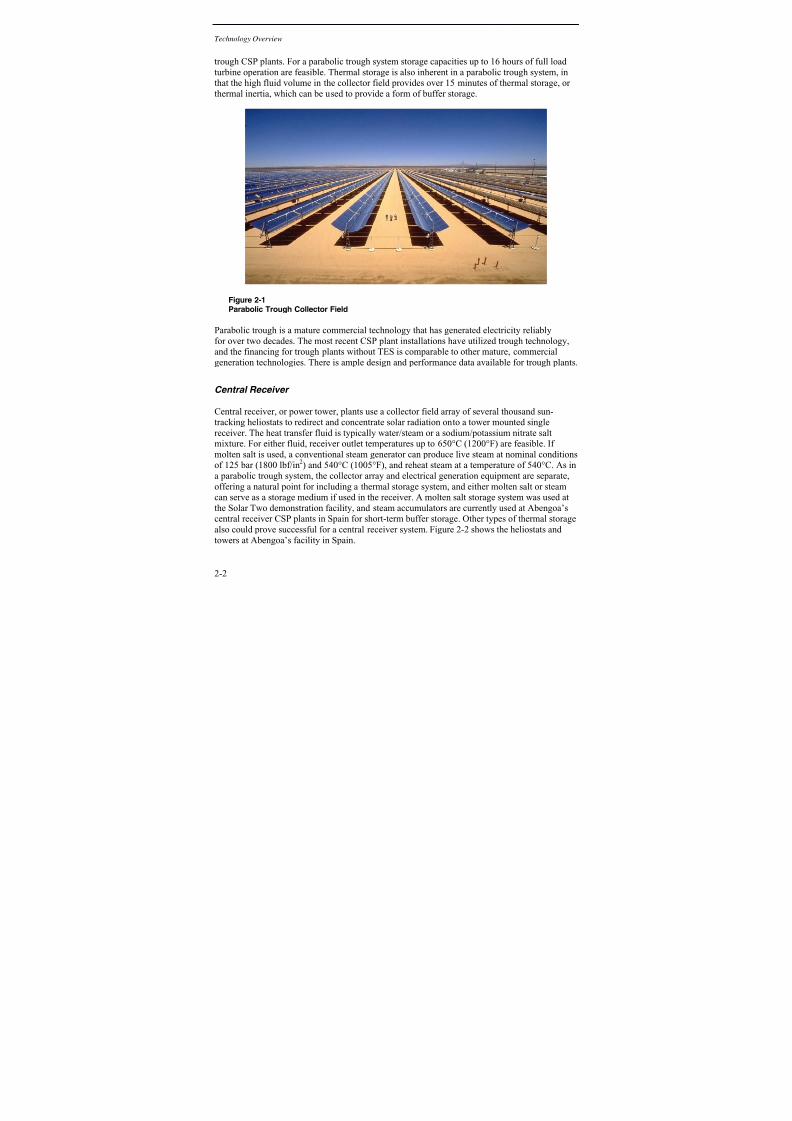
Parabolic trough plants use a field of linear parabolic collectors, shown in Figure 2-1, to redirect

and concentrate sunlight onto a tube receiver located at the focal line of the mirrors. Eachcollector tracks the sun by rotation about a horizontal axis. The heat transfer fluid is typically asynthetic oil mixture with a maximum operating temperature of 390°C (735°F). With a syntheticoil HTF, the steam generator produces live steam at nominal conditions of 377°C (711°F) and 100 bar (1465 lbf/in2), and reheat steam also at a temperature of 377°C (711°F). An importantaspect of parabolic trough technology is that the electrical energy production is separated fromthe solar energy collection, creating a natural insertion point between these two elements for athermal energy storage system. Most thermal storage technologies are compatible with parabolic

7/15/2019 Solar Storage 1019581


Technology Overview

2-2

trough CSP plants. For a parabolic trough system storage capacities up to 16 hours of full load turbine operation are feasible. Thermal storage is also inherent in a parabolic trough system, inthat the high fluid volume in the collector field provides over 15 minutes of thermal storage, or thermal inertia, which can be used to provide a form of buffer storage.

Figure 2-1Parabolic Trough Collector Field

Parabolic trough is a mature commercial technology that has generated electricity reliablyfor over two decades. The most recent CSP plant installations have utilized trough technology,

and the financing for trough plants without TES is comparable to other mature, commercialgeneration technologies. There is ample design and performance data available for trough plants.

Central Receiver

Central receiver, or power tower, plants use a collector field array of several thousand sun-tracking heliostats to redirect and concentrate solar radiation onto a tower mounted singlereceiver. The heat transfer fluid is typically water/steam or a sodium/potassium nitrate saltmixture. For either fluid, receiver outlet temperatures up to 650°C (1200°F) are feasible. If molten salt is used, a conventional steam generator can produce live steam at nominal conditionsof 125 bar (1800 lbf/in2) and 540°C (1005°F), and reheat steam at a temperature of 540°C. As in

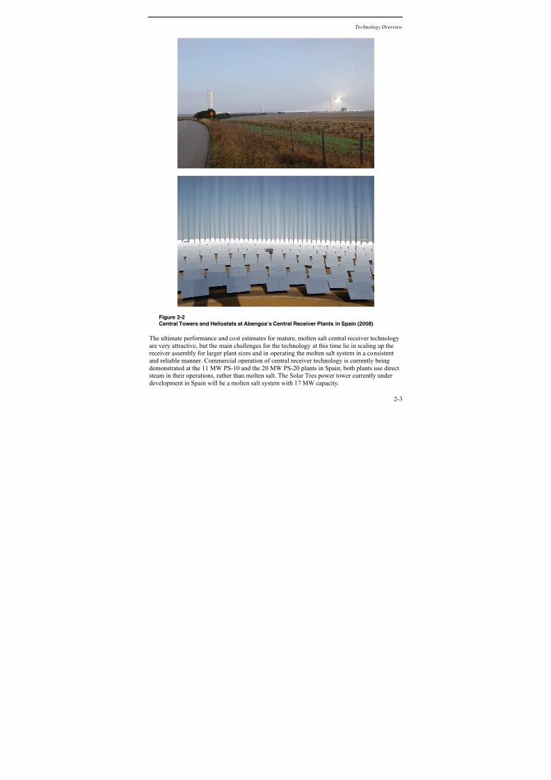
a parabolic trough system, the collector array and electrical generation equipment are separate,offering a natural point for including a thermal storage system, and either molten salt or steamcan serve as a storage medium if used in the receiver. A molten salt storage system was used atthe Solar Two demonstration facility, and steam accumulators are currently used at Abengoa’scentral receiver CSP plants in Spain for short-term buffer storage. Other types of thermal storagealso could prove successful for a central receiver system. Figure 2-2 shows the heliostats and towers at Abengoa’s facility in Spain.

7/15/2019 Solar Storage 1019581


Technology Overview

2-3

Figure 2-2Central Towers and Heliostats at Abengoa’s Central Receiver Plants in Spain (2008)

The ultimate performance and cost estimates for mature, molten salt central receiver technologyare very attractive, but the main challenges for the technology at this time lie in scaling up thereceiver assembly for larger plant sizes and in operating the molten salt system in a consistentand reliable manner. Commercial operation of central receiver technology is currently beingdemonstrated at the 11 MW PS-10 and the 20 MW PS-20 plants in Spain; both plants use directsteam in their operations, rather than molten salt. The Solar Tres power tower currently under development in Spain will be a molten salt system with 17 MW capacity.

7/15/2019 Solar Storage 1019581


Technology Overview

2-4

Thermal Energy Storage Operation

The primary purpose of thermal energy storage is to compensate for the sometimes variablenature of solar energy, as well as enabling operation of a solar energy system during times of the day when the sun is no longer available. The energy contained in the storage system can be

dispatched in any number of ways according to the desired output profile, but the strategies for using energy from storage fall into three main categories:

• Buffering power delivery

• Extending delivery period

• Displacing delivery period

Both two-tank TES and single-tank thermocline have the ability to extend or displace thedelivery of energy from the solar facility. Electrical utilities designate time-of-use (TOU) periodsfor electricity demand from customers; during periods of high demand, or on-peak times, themarket price of electricity is higher than during off-peak, or low demand periods. While solar

thermal power plants appear capable of providing energy for a large part of the on-peak TOU period, in some regions the on-peak period can extend well into the evening hours when solar facilities without storage are no longer capable of delivering energy. Two main options exist for altering the output of a solar thermal power plant to better match the load profile in locations thathave significant demand into the evening hours. The first operations strategy requires diverting a portion of the output from the collector field over the course of daily operation to charge thestorage system, which is then discharged once the sun has set to extend the delivery period.Alternatively, all of the energy output from the collector field can be used to charge the storagesystem at the beginning of daily operation, delaying plant startup until the storage system has been fully charged. The plant will then have sufficient energy in storage to continue operatingthrough the peak and into the evening use period. This strategy simply shifts the delivery period

a couple hours later into the day. Both of these storage options are depicted in Figure 2-3.

7/15/2019 Solar Storage 1019581


Technology Overview

2-5

Figure 2-3Displacement and Extension of Power Production using Thermal Energy Storage

3

Thermal Energy Storage Technologies

Two-tank and thermocline systems use sensible heat storage, in which the temperature of a liquid is raised without the material changing phase. They are considered active storage technologies,characterized by a storage medium that circulates through the storage system, and relies onforced convective heat transfer to move energy into and out of the storage medium. Nitrate saltsare the most common liquid storage media used in solar thermal energy systems.

3 Solar Millennium

7/15/2019 Solar Storage 1019581


Technology Overview

2-6

Two-Tank Indirect

The distinguishing feature of the two-tank indirect system is that the HTF that circulates throughthe collector field remains separate from the storage medium kept in the tanks. The HTF istypically a synthetic oil such as Therminol VP-1 (currently in use at the California SEGS plants

4)

or Dowtherm A, and the storage medium is likely to be molten salt. The system consists of a cold tank, normally operating at 290°C (554°F) or less, a hot tank, operating at temperatures up to390°C (703°F), the storage medium, the heat exchangers for transferring energy from the heattransfer fluid to the storage medium (and back), the storage medium pumps, and the associated balance of system equipment, such as an ullage gas system and electric heat tracing for allmolten salt components. Electric heat tracing is required to maintain inventory temperature in theevent of an extended plant outage, while the ullage gas system prevents oxidation of the storagemedium. A schematic diagram of a two-tank indirect system is shown in Figure 2-4.

Figure 2-4Two-Tank Indirect Thermal Storage System

The thermal energy storage system is charged by taking hot HTF from the solar field and runningit through the oil-to-salt heat exchangers. Simultaneously, cold molten salt is pumped from the

cold storage tank, and delivered to the heat exchangers. In the heat exchangers, the salt and theheat transfer fluid flow in a countercurrent arrangement. Heat is transferred from the HTF to thecold salt flowing through the heat exchanger, which leaves as hot salt that is then stored in thehot salt tank. When the energy in storage is needed, the flows of both the HTF and the salt are

4 S.D. Odeh, G.L. Morrison, and M. Behnia, “Thermal Analysis of Parabolic Trough Solar Collectors for ElectricPower Generation”, Darwin: ANZES Annual Conference, 1996.

7/15/2019 Solar Storage 1019581


Technology Overview

2-7

reversed in the oil-to-salt heat exchangers in order to reheat the HTF. Countercurrent flows in theheat exchangers are necessary in order to maximize heat transfer between the two fluids. Thereheated HTF is then used in the power block to generate steam to run the power plant.

The feasibility of the indirect system is proven and at present the concept is associated with the

lowest technological risk. However, the transfer of energy from the heat transfer fluid to the saltduring charging, and the transfer of heat from the salt to the heat transfer fluid duringdischarging, both require a temperature drop across the oil-to-salt heat exchanger. As such, thetemperature of the heat transfer fluid delivered to the steam generator when operating fromthermal storage is 10 to 20 °C lower than when operating directly from the collector field. Due totemperature and efficiency reductions associated with the heat exchangers, both the output and the efficiency of the Rankine cycle are unavoidably lower when operating from thermal storage.The round trip efficiency of a storage system is defined as the net electricity delivered from thestorage system divided by the amount of electricity that would have been generated from thesolar field thermal energy had it been directly converted to electricity. A typical efficiency for anindirect two-tank trough storage system is about 93 percent, whereas a future trough with a direct

two-tank molten salt storage system might be 98 percent efficient.

Two-Tank Direct

In a two-tank direct system, the fluid which circulates through the receiver of a power tower isalso used as the storage medium. Like the indirect system, the direct system consists of a cold tank and a hot tank, the storage medium and the associated balance of system equipment, such asthe electric heaters for inventory maintenance during plant outages. However, unlike the indirectsystem, this design uses the same fluid in both the storage system and the receiver, whicheliminates the need for a second set of heat exchangers used to transfer thermal energy between

the heat transfer fluid and the storage medium in the indirect system. When molten salt is used asthe storage medium, the cold and hot tanks can operate at temperatures up to 293°C (559°F) and 560°C (1040°F), respectively. A schematic diagram of the system is shown in Figure 2-5.

7/15/2019 Solar Storage 1019581


Technology Overview

2-8

Figure 2-5Two-Tank Direct Thermal Storage System

To charge the system, fluid from the cold tank is circulated through the receiver, and returned tothe hot tank. To discharge the system, fluid from the hot tank is circulated through the steamgenerator, and returned to the cold tank. All of the fluid from the receiver passes through the hotstorage tank. Depending on the residence time in the tank, the temperature of the fluid leavingthe tank is 0 to perhaps 1.5°C lower than the temperature entering the tank. As a result, the performance of the Rankine cycle in a plant with a two-tank direct storage system is essentiallythe same as a plant without thermal storage.

It may seem that only a single tank would be needed for the charged storage medium, but a cold tank is required to contain the volume of storage material that has already discharged its energyto the steam generator. During storage system discharging, the collector field will likely not bereceiving solar energy, although it is possible to charge and discharge simultaneously, as wasdemonstrated at Solar Two.

Two-tank direct TES systems will likely use a molten salt as the storage medium. Nitrate saltsare relatively inexpensive compared to synthetic oils and can provide tank storage capacityranging between 3 and 16 hours of full load turbine operation. The primary disadvantage to amolten salt storage system is the relatively high freeze point of typical nitrate salts. As such,

considerable care must be taken to ensure that the salt does not freeze in the solar field or elsewhere in the storage system. This includes installing an electric heat trace system on allequipment that comes in contact with the salt.

7/15/2019 Solar Storage 1019581


Technology Overview

2-9

Single-Tank Thermocline (Indirect or Direct)

Like the two-tank systems, a thermocline can operate either directly, with the storage mediumalso serving as the HTF in the collector field, or indirectly, with a separate storage media and

HTF. A thermocline system involves a single tank that is used to store both the hot and cold fluid, further reducing the cost of the TES system. This single-tank configuration features the hotfluid on top and the cold fluid at the bottom of the tank. The zone between the hot and cold fluidsis called the thermocline. While a thermocline can simply combine the hot and cold storagefluids into a single tank, the primary advantage of the thermocline storage system is that most of the storage fluid can be replaced with a low-cost filler material. This filler displaces the majorityof the molten salt that would be used in a comparable two-tank system, and provides a robust and inexpensive storage medium. A thermocline with a packed bed would actually be considered adual-media storage system, as it utilizes both a liquid and solid medium for storing energy.

To charge the system, hot fluid is introduced at the top of the tank, flows down through the

porous bed, and leaves from the bottom of the tank; in the process, heat is transferred from thehot fluid to the porous filler material. To discharge the system, the flow is reversed; cold fluid enters at the bottom of the tank, and is heated as the fluid flows up through the porous bed. Aschematic diagram of a direct thermocline system is shown in Figure 2-6. On the cold fluid sideof the tank, the system includes a bypass line to return cold fluid to the suction side of the pumpduring storage charging.

Figure 2-6Single Tank Direct Thermocline System

The principal liability for a thermocline is a fluid-to-solid media heat transfer coefficient whichis necessarily less than infinite. As a result, a thermal gradient is established in the storage media,and the gradient can grow to occupy the entire height of the tank. To prevent the gradient from

7/15/2019 Solar Storage 1019581


Technology Overview

2-10

increasing to the full tank height, the temperature of the fluid leaving the tank at the end of adischarge cycle must be allowed to fall below the design collector field outlet temperature, and the temperature of the fluid leaving the tank at the end of a charge cycle must be allowed to riseabove the design collector field inlet temperature. Figure 2-7 shows the performance of both adirect and indirect thermocline system at the end of a 3-hour charge cycle and at the end of a

discharge cycle. As predicted, the temperature at the tank outlet decays below the collector field outlet temperature throughout the discharge cycle, while the tank inlet temperature graduallyrises above the collector field inlet throughout the charge cycle.

Figure 2-7Indirect and Direct Thermocline Fluid Temperatures during Storage System Charging andDischarging

Thus, as the temperatures entering and leaving the thermocline tank diverge from the designtemperatures, the operation of the thermocline tank will influence the performance of both theRankine cycle and the collector field. Further, the magnitude of the effect will depend on thecoincident output of the Rankine cycle, and the coincident thermal output of the collector field.In addition, the degree to which the thermocline is subjected to a full or partial charge cycleduring the day, and a full or partial discharge cycle at the end of a day, will influence the shapeand the size of the thermal gradient the following day. Further discussion of thermocline performance is included in Chapter 5.

Operating Experience

The two-tank direct and indirect storage systems are the only thermal energy storage systems tohave seen commercial operation at a grid-connected CSP plant. The two-tank indirect system is

275

300

325

350

375

400

0.0 0.5 1.0 1.5 2.0 2.5 3.0

Time, Hours

F l u i d T e m p e r a t u r e ,

C

.

To Rankine - Direct To Field - Direct To Rankine - Indirect To Field - Indirect

7/15/2019 Solar Storage 1019581


Technology Overview

2-11

the closest to achieving commercial status, with one unit now operational at the Andasol 1 plantin Spain, and more either under construction or planned for operation in the next few years. Therest of the storage system concepts have undergone testing as prototypes and are poised to become commercial ventures with further research and development. For most of these systemsin the demonstration stage, a pilot plant presents the logical next step required for achieving

technological maturity.

Several early storage systems used oil as the storage fluid. Oils are not practical for futurecommercial projects for several reasons. The maximum operating temperatures are limited to300-400°C (570-750°F) due to thermal degradation. The lower operating temperatures relative tomolten salt central receiver systems means the steam cycles have lower Rankine conversionefficiencies. Even at these operating temperatures oils have a fairly high vapor pressure. A pressurized vessel would be required if oil were used as the thermal storage medium. Pressurized tanks can significantly increase the cost of the TES system, and the large tank sizes required tostore thermal energy in this temperature range could make the TES prohibitively expensive.Pressurized tanks of oil also pose a fire hazard. The commodity prices of synthetic oils are too

high for them to be considered as storage fluids. Molten salt and water are lower cost fluid options, and molten salt has the benefit of atmospheric pressure operation.

National laboratories, particularly in Europe and the U.S., are investing heavily in thermalenergy storage research. The U.S. Department of Energy has awarded 15 grants totaling up to$67.6 million dollars for FY 2009. The projects cover a broad range of TES technologies,including the proposed construction of a prototype thermocline system at the Arizona PublicService CSP plant in Red Rock, AZ, solid media storage, thermochemical storage and phasechange materials. Through these grants and other renewable research, the DOE intends to spur the commercialization and deployment of solar technologies and to reduce the levelized cost of electricity generated at CSP facilities. The DOE goals include reducing the LCOE from 13-16cents/kWh today with no storage to 8-11 cents/kWh with 6 hours of thermal storage capacity by2015, and to less than 7 cents/kWh with 12-17 hours of thermal storage by 2020.5

Two-Tank Indirect

The two-tank indirect system has recently been proven at large scale. The first large scalecommercial system was commissioned in early 2009 at the Andasol 1 plant in Spain. Thetechnology is expected to be commercially viable and is considered the current state-of-the-art inthermal energy storage systems. Andasol 2 was commissioned in late 2009. Both plants have1010 MWht storage capacity, providing roughly 7.5 hours of full power output at 50 MWe. TheAndasol storage systems represent an important step towards incorporating thermal energy

storage into CSP plants – the performance data from these plants will provide a valuable sourceof information for future thermal storage systems, and the knowledge and experiences gained will help pave the way for future two-tank TES systems. Andasol 3 is currently under construction with an identical TES system, and other plants with the same design are indevelopment. Figure 2-8 shows the Andasol 1 storage tanks during construction.

5 Department of Energy, “ DOE Funds 15 New Projects to Develop Solar Power Storage and Heat Transfer ProjectsFor Up to $67.6 Million”, http://www.energy.gov/news/6562.htm, 2008.

7/15/2019 Solar Storage 1019581


Technology Overview

2-12

Figure 2-8

Thermal Storage Tanks under Construction at Andasol 1 (2007)

In addition to the Andasol storage systems, Arizona Public Service has contracted Abengoa todesign and build a plant that will include an indirect thermal storage system using molten salt asthe storage medium. As of this publication, ground breaking was scheduled for late 2010. TheSolana plant will be located near Gila Bend, Arizona and will provide 280 MW of electricity toAPS customers. The design uses a molten salt storage system consisting of six to eight storagetanks (three to four pairs of hot and cold tanks) with the capability for six hours of full load operation. Figure 2-9 shows the proposed layout for the Solana plant; the molten salt storagetanks are labeled “5” in the figure.

Figure 2-9Artist’s Rendering of APS Solana Power Plant; Molten Salt Storage Tanks are Labeled “5”

6

6 Arizona Power Service, “About Solana Generating Station” ,http://www.aps.com/main/green/Solana/Technology.html, © 1999-2009

7/15/2019 Solar Storage 1019581


Technology Overview

2-13

With the multiple TES systems at Andasol in operation and the APS Solana plant planned for 2009, the two-tank indirect storage system will likely be the first TES technology to achieve fullcommercial status, and can be considered the state of the art for thermal energy storage systems.

Two-Tank Direct

The SEGS I system included a 110-MWht two-tank direct TES system that was used in plantoperation from 1985-1999. SEGS 1 used Caloria, a type of mineral oil, as both the HTF in thecollector field and the storage medium. In 1999, the storage tanks were completely destroyed when the flammable oil caught on fire. Like other thermal energy storage systems that are either in the pre-commercial prototype or demonstration stages, the SEGS I TES was a one-of-a-kind storage system, and was not included in any of the later SEGS facilities. In SEGS II-IX Caloriawas replaced by higher-temperature Therminol oil in the collector field, but since Therminol isdifficult to store due to its higher vapor pressure at the operating temperatures in the plant, thelater SEGS systems did not include thermal energy storage systems.

A two-tank molten salt storage system was first used at the Themis central receiver plant inFrance in the late 1980s. It used circular-horizontal hot and cold tanks with a total capacity of 40 MWht. Hitec salt was used in the receiver and storage system. In 1996 another centralreceiver project, Solar Two, demonstrated the same direct molten salt concept except with twovertical cylindrical tanks. This design provided the foundation for current two-tank molten saltthermal storage systems. Figure 2-10 shows the two-tank direct molten salt TES system at Solar Two, which has since been dismantled.

There are several direct central receiver projects in various stages of development. Gemasolar (also known as Solar Tres) is currently under construction in Spain and is expected to be runningin mid-2011. The plant is 17 MW and will have 15 hours of storage capacity using the two-tank

direct molten salt approach. SolarReserve recently announced power purchase agreements for three central receiver projects that are considerably larger, but will employ similar two-tank direct storage technology. The SolarReserve plant generation capacities range from 50 MW to150 MW and will have a minimum of 7 hours of storage capacity. The 50 MW plant in Spainwill have sufficient capacity to operate up to 24 hours a day with an annual capacity factor of about 80%.

7/15/2019 Solar Storage 1019581


Technology Overview

2-14

Figure 2-10Thermal Energy Storage System at Solar Two, Barstow, CA

The Italian National Agency for New Technologies, Energy and the Environment (ENEA) has been testing molten salt in a Solar Collector Test Loop facility since 2004 to study the effects of molten salt on the valves and other process components of a parabolic trough installation. After more than 2000 hours of operation and approximately 200 fill and drain cycles, ENEA reported that no major obstacles to molten salt operation in the test collector loop were encountered.According to ENEA, further research is needed to fully characterize such items as the sealingand gasket materials and any rotating joints that come into contact with the molten salt.

While conducting the collector loop tests, ENEA simultaneously developed a design for a pilot project, dubbed Archimede, which will integrate a parabolic trough and a direct two-tank TESsystem with a combined-cycle plant, using molten salt as the HTF. The project stalled due to adelay in receiving national subsidies for solar thermal power plants, but is expected to comeonline in 2010. Like Andasol for indirect systems, Archimede will be an important source of operating and performance data for a direct storage system.

For indirect trough TES applications, the cost of the oil-to-salt heat exchanger is high due to thelarge surface area needed for the low approach temperature of the oil. Significant cost savingsare anticipated for direct trough storage systems if the collector field can be operated usingmolten salt as the HTF. Circulating molten salt through the collector field presents distinct

challenges in contrast to a central receiver plant. Salt freeze recovery and heat loss in thecollector field loops is a concern, as are the capabilities of the collector field processcomponents, such as the piping, valves, and pumps.

The high freezing point of molten salt remains an issue for both direct and indirect systems, introughs especially, and is the subject of current R&D efforts. Both the DLR and the DOE aredeveloping salts with much lower melting temperatures than those associated with the common

7/15/2019 Solar Storage 1019581


Technology Overview

2-15

binary nitrate salts, having achieved melting points as low as 100°C (212°F)7, and they are performing experiments with these salts to study freeze recovery

8. The Department of Energy

has also awarded grants for near-term development of advanced heat transfer fluids, includingfunding for projects that will attempt to develop low melting point eutectic salt mixtures.

Single-Tank Thermocline (Indirect or Direct)

The Solar One central receiver project included a 182 MWht indirect mineral oil thermoclinesystem which began operating in 1982. It was shut down when a steam explosion caused a smallrupture of the thermocline tank in 1988. Although the resulting fire was extinguished relativelyquickly and with minimal damage, the storage tank was not reused. A single-tank thermoclineusing thermal oil has also been successfully tested at the Plataforma Solar de Almería, one of Europe’s most prominent CSP research facilities. The PSA thermocline is a component of theSmall Solar Power Systems – Distributed Control System (SSPS – DCS), which includes a parabolic trough collector field and a Multi-Effect Distillation (MED) desalination plant inaddition to the thermal energy storage system. The direct thermocline systems uses dual-media

storage; Therminol 55 from the collector field is the storage fluid and a metal filler inside thetank stores the heat. The system provides up to 5 MWht storage capacity. Although thethermocline testbed has been operating successfully since the early 1980’s, no plans for further commercial development of this system are proposed at this time.

In 2001, Sandia National Laboratories successfully demonstrated a 2.3-MWht, packed-bed thermocline storage system with binary molten salt fluid and quartzite rock and sand filler material.

9In developing the design of the thermocline testbed, Sandia evaluated various filler

materials and found that a quartzite and sand mixture was an economical and practical choiceand that both materials were able to withstand immersion in an isothermal molten salt bath aswell as repeated thermal cycling tests with molten salt. Relatively simple cost analyses were

conducted to evaluate the costs of materials, molten salt and filler materials for a larger commercial-scale thermocline TES system. The analyses showed that thermocline-based energystorage configurations may offer the least-cost energy storage option, being about 35 percentcheaper than a similar-sized two-tank TES system. The system studied by Sandia sought toimprove on the indirect two-tank storage system concept, but a thermocline concept could also be applied to a direct system, and, like the two-tank system, will benefit from molten salt HTFresearch.

A single-tank direct thermocline storage system was proposed and designed for the 1 MWSaguaro parabolic trough power plant owned by Arizona Power Service. The plant began

7 Brosseau, D. and Kolb, G., “Sandia Thermal Storage Activities”, Presented at Trough Workshop, Golden, CO.2007.

8 G. Kolb, C. Ho, B. Iverson, T. Moss, and N. Siegel, “Free-thaw Tests of Trough Receivers Employing a MoltenSalt Working Fluid”, Proceedings of 2010 ASME Energy Sustainability Conference, ES2010-90040, Sandia National Laboratories, Albuquerque, NM, May 2010.

9 D.A. Brosseau, P.F. Hlava, and M.J. Kelly, “Testing Thermocline Filler Materials and Molten Salt Heat Transfer Fluids for Thermal Energy Storage Systems Used in Parabolic Trough Solar Power Plants”, Albuquerque, NM2004.

7/15/2019 Solar Storage 1019581


Technology Overview

2-16

operation in December 2005 without a TES system, but APS and the national labs beganstudying options for retrofitting the plant to include six hours of thermal storage in order to provide electricity during the evening peak period. A design and cost estimate for the system wasdeveloped by Nexant, Inc. and Sandia National Laboratories provided a performance analysis of the proposed system. Both studies indicated that the thermocline was a viable option for the

Saguaro plant, and a recent grant from the DOE will be used to build and test the thermoclinestorage system. The project is one of three thermal storage systems that will be incorporated intoan operational power plant as part of this research phase. The results of the Saguaro project will provide much-needed performance data and operations experience for a thermocline system.

Development Status

Only the two-tank technologies have been demonstrated in commercial operation, and although a two-tank direct system using Caloria oil was successfully operated for fourteen yearsat SEGS I, systems using molten salt as the storage medium have yet to see continuous long-term

commercial operation. Both the compatibility of the raw materials and the long-term durability,reliability, and performance of critical components of thermal storage systems using molten saltremain uncertain. Extended operation of molten salt systems in addition to further testing and research will be required to complete commercial development and to fully characterize thetechnical constraints on molten salt TES.

Thermocline technology would benefit greatly from operation and testing at a non-commercial pilot plant, much like Solar Two, or by simply incorporating a storage system into an operationalCSP plant, as Arizona Public Service intends to do at the Saguaro plant. Although the oilthermocline at the PSA has performed well, the molten salt thermocline has yet to see any testing beyond the prototype studied at Sandia National Laboratories, and a full-scale pilot system

integrated with a CSP plant will permit further observation and validation of this concept.Table 2-1 has a summary of current development needs for two-tank and thermoclinetechnologies.

7/15/2019 Solar Storage 1019581


Technology Overview

2-17

Table 2-1Current Development Needs for Thermal Storage Technology

StorageTechnology

Development Needs

Two-Tank Indirect • Operating experience from the planned commercial facilities (Andasol,Solana)

• More units in commercial operation

• An established supply-chain for system components

• Evaluation of long-term durability and reliability of materials in use withmolten salt

Two-Tank Direct • Validation of molten salt operation in a full-sized collector field

• Operation and evaluation of a commercially operated unit

• Evaluation of long-term durability and reliability of materials in use withmolten salt

Single-Tank

Thermocline(Direct or Indirect)

• Improved modeling techniques, including an effective method for sizing the

thermocline tank

• A pilot plant or commercially operated unit

• Thermal ratcheting assessment

7/15/2019 Solar Storage 1019581


7/15/2019 Solar Storage 1019581


3-1

3 THERMOCLINE DESIGN AND OPERATION

Design Basis

Initially four storage capacities were modeled for both indirect trough and direct central receiver systems for a total of eight design cases. Over the course of the analysis, the largest possiblesingle-tank sizes were identified as roughly 1500 MWht for the indirect trough and 3500 MWht for the direct central receiver. Two additional design cases were developed to show the full rangeof tank sizes that may be feasible for this technology. Although cost estimates were not

specifically developed for the 1500 MWht direct central receiver and the 3500 MWht indirect parabolic trough, cost estimates can reasonably be extrapolated or interpolated for thesecorresponding cases. Table 3-1 contains a summary of all the design cases considered.

Table 3-1EPRI Thermocline Molten Salt Energy Storage Design Cases

Design Case MWht Maximum TESTemperature

Technology

1 400°C (752°F) Indirect Trough

2100

560°C (1040 °F) Direct Central Receiver


4500



61000



83000



10*1500


11* 400°C (752°F) Indirect Trough

123500


* Values were interpolated or extrapolated from other design case results

7/15/2019 Solar Storage 1019581


Thermocline Design and Operation

3-2

The selected storage fluid for all cases was a binary sodium/potassium nitrate salt mixture(60% NaNO3/40% KNO3). It is likely that any future system incorporating a liquid storage mediawill use molten salt, with the exception of steam storage, which can be used for short-term buffer storage. Therminol is the most common heat transfer fluid in parabolic trough systems, and itsmaximum operating temperature is limited due to thermal degradation. Consequently the

maximum inlet temperature for the molten salt storage fluid was set as 400°C (752°F) for theindirect trough storage systems in this study. For central receiver systems, the maximumtemperature was set by the thermal degradation temperature of the molten salt; the inlet storagetemperature was set as 560°C (1040°F).

Design Conditions

The complete thermocline storage system design requirements are presented in Appendix A. Themajor assumptions include the following:

• Molten salt temperature at solar receiver inlet (direct and indirect systems): 293°C (559°F)

• Six hours storage (solar multiple is approximately 1.8)

• Void fraction is 25%

• Barstow, California is assumed as the basis for cost and weather conditions

High level design considerations include:

• Structural integrity of tank and foundation

• Thermal analysis of tank and connected auxiliary hot piping systems

• Tank height/diameter ratio optimization (multiple modular thermocline tanks possible)

• Wall material

• Thermal insulation

• Heat tracing

Design details considered:

• Design of tank pressure boundary as per API standards

• Basic foundation design

• Upper, auxiliary and lower manifold designs to minimize entrainment

• Ullage space

• Pumps

• Piping

• Valves

• Heat exchangers

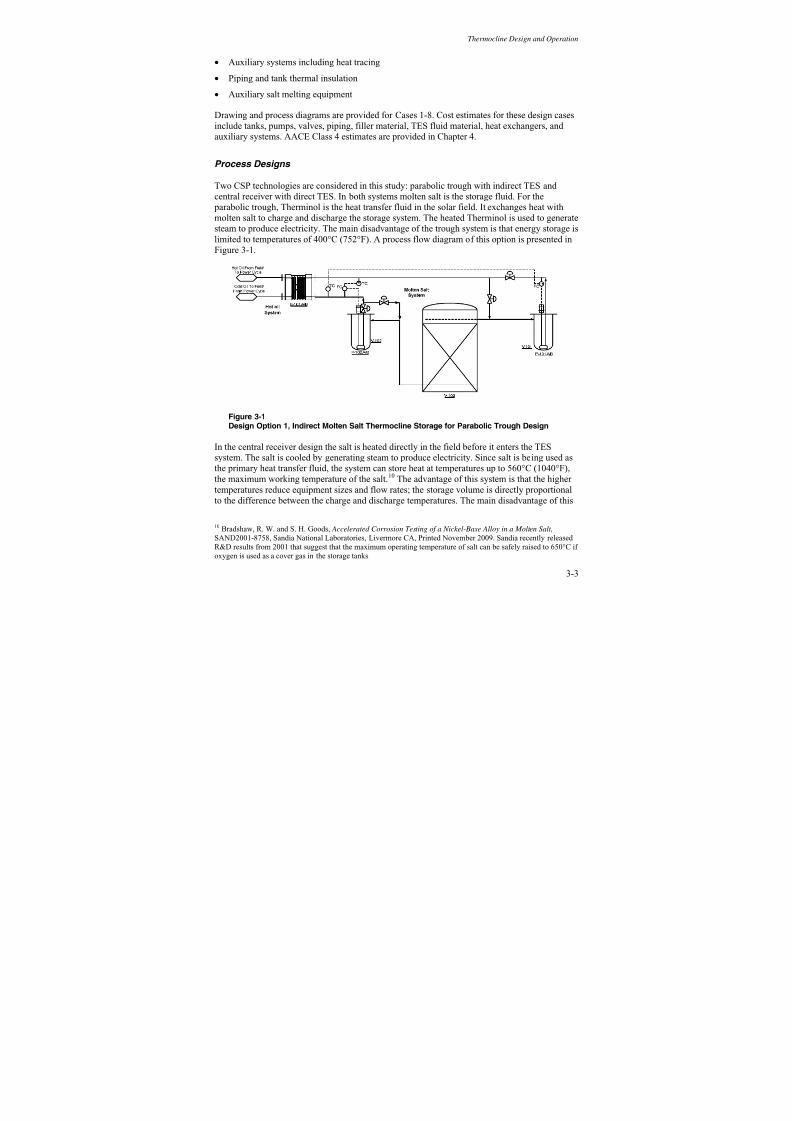
7/15/2019 Solar Storage 1019581



3-3

• Auxiliary systems including heat tracing

• Piping and tank thermal insulation

• Auxiliary salt melting equipment

Drawing and process diagrams are provided for Cases 1-8. Cost estimates for these design casesinclude tanks, pumps, valves, piping, filler material, TES fluid material, heat exchangers, and auxiliary systems. AACE Class 4 estimates are provided in Chapter 4.

Process Designs

Two CSP technologies are considered in this study: parabolic trough with indirect TES and central receiver with direct TES. In both systems molten salt is the storage fluid. For the parabolic trough, Therminol is the heat transfer fluid in the solar field. It exchanges heat withmolten salt to charge and discharge the storage system. The heated Therminol is used to generatesteam to produce electricity. The main disadvantage of the trough system is that energy storage is

limited to temperatures of 400°C (752°F). A process flow diagram of this option is presented inFigure 3-1.

Figure 3-1Design Option 1, Indirect Molten Salt Thermocline Storage for Parabolic Trough Design

In the central receiver design the salt is heated directly in the field before it enters the TESsystem. The salt is cooled by generating steam to produce electricity. Since salt is being used asthe primary heat transfer fluid, the system can store heat at temperatures up to 560°C (1040°F),

the maximum working temperature of the salt.10 The advantage of this system is that the higher temperatures reduce equipment sizes and flow rates; the storage volume is directly proportionalto the difference between the charge and discharge temperatures. The main disadvantage of this

10 Bradshaw, R. W. and S. H. Goods, Accelerated Corrosion Testing of a Nickel-Base Alloy in a Molten Salt,

SAND2001-8758, Sandia National Laboratories, Livermore CA, Printed November 2009. Sandia recently released R&D results from 2001 that suggest that the maximum operating temperature of salt can be safely raised to 650°C if oxygen is used as a cover gas in the storage tanks.

7/15/2019 Solar Storage 1019581



3-4

process is that it requires more expensive materials due to the higher temperatures. A processflow diagram of this option is presented in Figure 3-2. Complete process flow diagrams for boththe indirect and direct systems are given in Appendix B.

Figure 3-2Design Option 2, Direct Molten Salt Thermocline Storage for Central Receiver Design

Tank Sizing

Thermocline tanks were sized using the method designed by Zhen Yang and Suresh Garimella11

.In this method, a tank diameter is assumed and the energy density of the tank is determined bydividing the desired power generation by the area of the cross section. This can then be used tosolve for the Reynolds number using Appendix C.

Pr Re,

s

chcl

d

T T k

A

P −= Equation 3-1

In this equation P is the power generation, A is the horizontal cross-sectional area of the tank, k l,c is the thermal conductivity of the salt, Th is the temperature of the hot salt, Tc is the temperatureof the cold salt, d s is the diameter of the tank, Re is the Reynolds number, and Pr is the Prandtlnumber. Since the Prandtl number is a known constant, it is possible to solve this equation for the Reynolds number.

The next step is to calculate the stored thermal energy of the tank per unit area. This makes it

possible to solve for the non-dimensional useful energy (Hη95) as shown in Equation 3-2.

( )[ ] ( ) 95,, 1 η ρ ε ερ H d T T T C C A

Qschhs pss pl −−+= Equation 3-2

11 Yang, Z., Garimella, S.V. “Thermal Analysis of Solar Thermal Energy Storage in a Molten-salt Thermocline,”Solar Energy, Vol. 84, 2010, pp. 974-985.

7/15/2019 Solar Storage 1019581



3-5

In this equation Q is the useful energy extracted from the tank, ε is the void fraction, ρ is density,and C p is the specific heat capacity at constant pressure, H is the tank height divided by the filler

size (nondimensional variable), and η95 is the efficiency. The subscripts l and s refer to themolten salt liquid and the solid filler, respectively. The efficiency is based on a 95% allowablethreshold between the lower and upper temperature limits of the molten salt stored. Under this

thermal constraint, any salt outflow with temperature below the 95% threshold is considered notuseful for steam generation (just as one example of a cut-off). This value is somewhat arbitrary,chosen to reflect the inherent thermal degradation of the discharge process with time. If colder temperatures are viable for steam generation, the threshold should be lowered to reflect greater flexibility of the thermocline tank operation. This in turn would increase the discharge efficiencyof a given tank as more of the energy extracted is considered useful. Figure 3-3 shows the changein efficiency for a tank of fixed height and Reynolds number as a function of minimum allowabledischarge temperature. As the allowable discharge temperature is lowered, the dischargeefficiency increases (going to the left of the x-axis).

Figure 3-3Efficiency Curve as a Function of Allowable Discharge Temperature

Once Hη95 is known the efficiency is assumed to be 100% and H is calculated. Then the

efficiency is calculated from Equation 3-3.

485.0Re00055.0Re00234.0

1801.0

95

6151.0

100Re1807.01

−+−

⎟ ⎠

⎞⎜⎝ ⎛ −=

H η Equation 3-3

7/15/2019 Solar Storage 1019581



3-6

This efficiency is substituted into the previous calculation, and the final result is determined through multiple iterations until the height of the tank converges on a single value. This height isthe minimum height required to provide the design power generation while also maintaining astable thermocline. It can be seen from repeated calculations that taller tanks with smaller diameters have the highest efficiencies if the tanks are of equal volume. For a fixed tank height

tanks of different diameters will perform identically under adiabatic conditions.

This approach implies that taller tanks are preferred. However, there are many designconsiderations that limit the height of the tank such as the maximum bearing capacity of the soil and earthquake code requirements. A civil engineering study was performed using soilinformation for Barstow, California.12 Due to the density of the salt and quartzite-sand mixture,it was determined that the maximum liquid level in the tank should be limited to 39 ft. Thedetails of this study are included in Appendix D. This is the maximum height that can besupported by a typical foundation, and it was used for the basis of the thermocline design. If a10% oversized foundation is designed (above 150’ in diameter), it is possible to support a moltensalt level up to 49 ft (50 ft tank height). A figure showing the maximum thermocline capacity for

standard and oversized foundations is presented in Appendix K.

No active convection cooling is required in the assumed civil foundation design. The insulation bricks and lower temperature salt at the bottom of the tank limit the concrete temperature well below 100°C (212°F) for both the parabolic trough and the central receiver thermocline designs.

Material Selection

The binary molten salt used in this project was assumed to be a mixture of sodium nitrate and potassium nitrate. This compound is corrosive in the presence of liquid water. However there is

little to no water present at the process conditions. As a result, material selection is driven only by the temperature and pressure requirements of the process.

All equipment and tanks that operate below 800°F (427°C) were assumed to use hightemperature carbon steel SA-285-C. This includes all piping and surge tanks, as well as the head and base plate of the tanks. This material is well suited to the service, and is very cost effective.

All equipment and tanks operating above 800°F (427°C) were assumed to be composed of Stainless Steel 347 (SA-240-347). This material has been historically used in this service;however, there is a slight risk of material sensitization. Black & Veatch recommends a materialstesting program be completed to further qualify the material for use in the final design. A

discussion of sensitization and its potential impact is presented in Appendix E.

Tank Design

The final height of the tank was assumed to be 40 feet for all of the original design cases exceptCase 8, in which the larger foundation permitted constructing a tank 47 feet tall. All of the tanks

12 “Environmental Conditions Barstow, California”

7/15/2019 Solar Storage 1019581



3-7

are designed with 1 foot of ullage space available at the top to accommodate thermal expansion,as well as 3 feet of molten salt at the top to provide space for the distribution manifold. Theremainder of the tank is filled with quartzite packing and molten salt. A summary of results is presented in Table 3-2. Results for the additional design cases (9-12), representing the maximumfeasible single-tank sizes for indirect and direct systems, can be found in Appendix J. Based on

industry experience, a maximum practical tank diameter of 160 feet was assumed. Completesizing information for all of the remaining process equipment (surge tanks, heat exchangers, pumps) is provided in Appendix F.

Due to the heating and cooling of the salt, the liquid level in the tank will vary over time. At560°C (1040°F) the salt will have a liquid level of 39 feet, providing 3 feet of heel in the tank above the hot molten salt nozzle. When the salt is cooled to 293°C (559°F), it will loseapproximately 10% of its volume. If the entire vessel were cooled to 293°C, the salt would lose 1foot 3 inches of height.

Table 3-2Summary of Molten Salt Thermocline Storage Tank Sizes

Design Case MWht Number of TanksTank Height

(ft)Tank Diameter

(ft)

1 Indirect Trough 1 40 48

2 Direct Central Receiver100

1 40 31



1 40 69


6 Direct Central Receiver

1000

1 40 987 Indirect Trough 2 40 160


1 47 155

For cost comparison purposes, a two-tank thermal energy storage system was designed as well asthe thermocline system. The two-tank TES system is similar to the thermocline system, exceptthe single thermocline tank and the surge tanks are replaced with two molten salt tanks. Onemolten salt tank holds cold salt at 293°C (559°F), and the other molten salt tank holds salt ateither 400°C (752°F) or 560°C (1040°F) depending on the design case. The sizes for theequivalent capacity two-tank systems are provided in Table 3-3.

7/15/2019 Solar Storage 1019581



3-8

Table 3-3Summary of Molten Salt Two-Tank Storage Tank Sizes

Design Case MWht

Number ofTwo-Tank

Sets

Tank Height(ft)

Cold Tank Diameter

(ft)

Hot Tank Diameter

(ft)

1a Indirect Trough 1 46 35.5 36.5

2a Direct Central Receiver100

1 46 22.5 23

3a Indirect Trough 1 46 78.5 81.5


1 46 50 51.5

5a Indirect Trough 1 46 111 115


1 46 70.5 73

7a Indirect Trough 2 46 136 141

8a Direct Central Receiver

3000

1 46 122 126

Heat and Material Balance

Molten salt flow rates are presented in Table 3-4. The charging salt flow is the amount of saltheated by the solar collector field. The discharging salt flow is the amount of salt used to produceelectricity. For the purposes of this design, a solar multiple of 1.8 was assumed. A detailed heatand material balance containing physical properties and the different operating modes is presented in Appendix C.

Line sizes for the system are presented in Table 3-5. Line sizes were calculated to provide

pressure drops below 1 psi per 100 feet of pipe. For the purposes of line sizing, all pipes areassumed to be schedule 40.

Table 3-4Molten Salt Flow Rates

Design CaseThermal

Storage (MWh)Charging Molten Salt Flow

(lb/hr)Discharging Molten Salt Flow

(lb/hr)

1 Indirect 100 1,488,444 826,913

2 Direct 100 596,493 331,385

3 Indirect 500 7,442,220 4,134,567

4 Direct 500 2,982,463 1,656,924

5 Indirect 1000 14,884,441 8,269,134

6 Direct 1000 5,964,926 3,313,848

7 Indirect 3000 44,653,323 24,807,402

8 Direct 3000 17,894,777 9,941,543

7/15/2019 Solar Storage 1019581



3-9

Table 3-5System Line Sizes

Design Case Charging Line Size (inches) Discharging Line Size (inches)

1 Indirect 10 8

2 Direct 8 6

3 Indirect 20 16

4 Direct 14 12

5 Indirect 24 20

6 Direct 18 16

7 Indirect 36 30

8 Direct 26 20

Insulation

A data sheet for the thermocline tank is attached in Appendix K. This data sheet shows themechanical details considered in the design of the vessel and the fundamental design of the shelland vessel head. Insulation is required both for personal protection and to minimize the operatingcosts of the facility. Mineral wool was selected as insulation because it is suitable for the hightemperatures of the tank and because it offers the best process economics. The thickness of theinsulation was optimized to minimize project costs. These costs were estimated assuminginsulation prices of $1.71/ft

2for a 2-inch-thick board of insulation. Labor costs were assumed to

be $38.25/hr, which is typical for California. Power prices were assumed to be $0.35 per kWheand prices were assumed to escalate at 3% per year. Capital costs were depreciated over a period

of 5 years, which is typical for renewable energy projects. The final insulation thicknesses are presented in Table 3-6.

Table 3-6Summary of Insulation Thickness

Service Temperature Thickness (in)

Cold Salt 288°C (550°F) 15

Hot Salt (Trough Design) 400°C (752°F) 17

Hot Salt (Power Tower Design) 560°C (1050°F) 23

Impoundment Wall Design

In order to ensure molten salt containment in the event of a tank failure, an impoundment wallmust be constructed around the thermocline tank. Figure 3-4 shows a general arrangement of thisdesign. The impoundment wall would be constructed from compacted soil and is designed tocontain the complete volume of the tank, including molten salt and quartzite rock.

7/15/2019 Solar Storage 1019581



3-10

Thermocline Tank(V-103)

40'

V-101 V-102

20 feet 20 feet

ImpoundmentWall

40'

Figure 3-4General Arrangement of the Impoundment Wall

The minimum distance from the thermocline tank to the impoundment wall is 40’. This distancewas selected following the guidelines provided by NFPA 59A. Impoundment wall dimensionsare provided in Table 3-7. This information is to be taken as a general guideline, and should beconfirmed in a detailed design.

Table 3-7Impoundment Wall Design Information

Case Wall Height (ft) Distance From Tank (ft)

1 Indirect 4.5 40

2 Direct 2.5 40

3 Indirect 10 40

4 Direct 7 40

5 Indirect 13 40

6 Direct 10 40

7 Indirect 13 40

8 Direct 10 45

7/15/2019 Solar Storage 1019581



3-11

Thermocline Distributors Design

The molten salt distributors are critical to the operation of the thermocline. The intended role of the distributors is to provide a uniform distribution of the molten salt flow over the entire cross-

sectional area of the tank. This is necessary to maintain the separate temperature regions withinthe tank. A sketch of the proposed upper and lower distributor designs is given in Figure 3-5.

Figure 3-5Thermocline Distributor Design

Additional details about the feeder pipe are provided in Figure 3-6. The bottom feeder pipe usesa larger guard pipe to support the weight of the quartzite material. The larger pipe is screened toremove quartzite from the molten salt. The top feeder pipes do not require a supporting external pipe, and simply rest on top of the quartzite rock. A sketch showing the manifold arrangement,as well as the nozzle placement and thermocouple placement is provided in Appendix M.

7/15/2019 Solar Storage 1019581



3-12

Figure 3-6Thermocline Distributor Feeder Pipe Design

An orifice density of 3 holes per square meter was assumed to ensure adequate circulation of themolten salt. The orifice diameter is 0.5 inches, which was selected to minimize plugging of thedistributor due to the presence of quartzite fines. A hydraulic analysis was completed on thedistributor and the recommended pipe sizes are given in Table 3-8. It was assumed that screeningmaterial could be placed over the orifice holes to prevent sand from entering the distributor. Thisinformation is preliminary, and a detailed analysis of the distributor will need to be completed inthe future in order to ensure proper separation and support of the quartzite material in thethermocline environment. This design is only a preliminary concept of the distributor, and further details will need to be determined through a detailed design. The distribution of theorifice holes will need to be optimized for uniform flow across the thermocline.

7/15/2019 Solar Storage 1019581



3-13

Table 3-8Distributor Pipe Size

Design Case1

Indirect2

Direct3

Indirect4

Direct5

Indirect6

Direct7

Indirect8

Direct

Inlet Pipe Diameter (in) 12 10 20 14 24 18 36 26

Header Pipe Diameter (in) 8 6 12 8 16 12 24 18

Feeder Pipe Diameter (in) 3 2 6 4 8 5 8 6

Number of distributionpoints 420 200 2,100 900 4,200 1,800 11,000 5,100

Total Pressure Drop (psi) 0.37 0.10 0.99 0.42 1.07 0.72 1.10 0.63

Purdue University also performed a CFD investigation of the distributor manifold design proposed for the thermocline system. The manifold model was applied to the eight original

proposed design cases to assess the uniformity of the outflow from the manifold into the fillerbed region. GAMBIT was used to mesh the distributor and the adjacent filler regions, as shown inFigure 3-7.

(a) Geometry (b) Mesh

Figure 3-7(a) Distributor and its Adjacent Regions, and (b) the Corresponding Mesh

The following equations govern the computation of distributor flow:

Flow in the tube region: The relation between pressure p and mean flow velocity um is expressed

below, where D is tube diameter, l the flow distance and λ the flow friction factor which isdetermined by Figure 3-8:

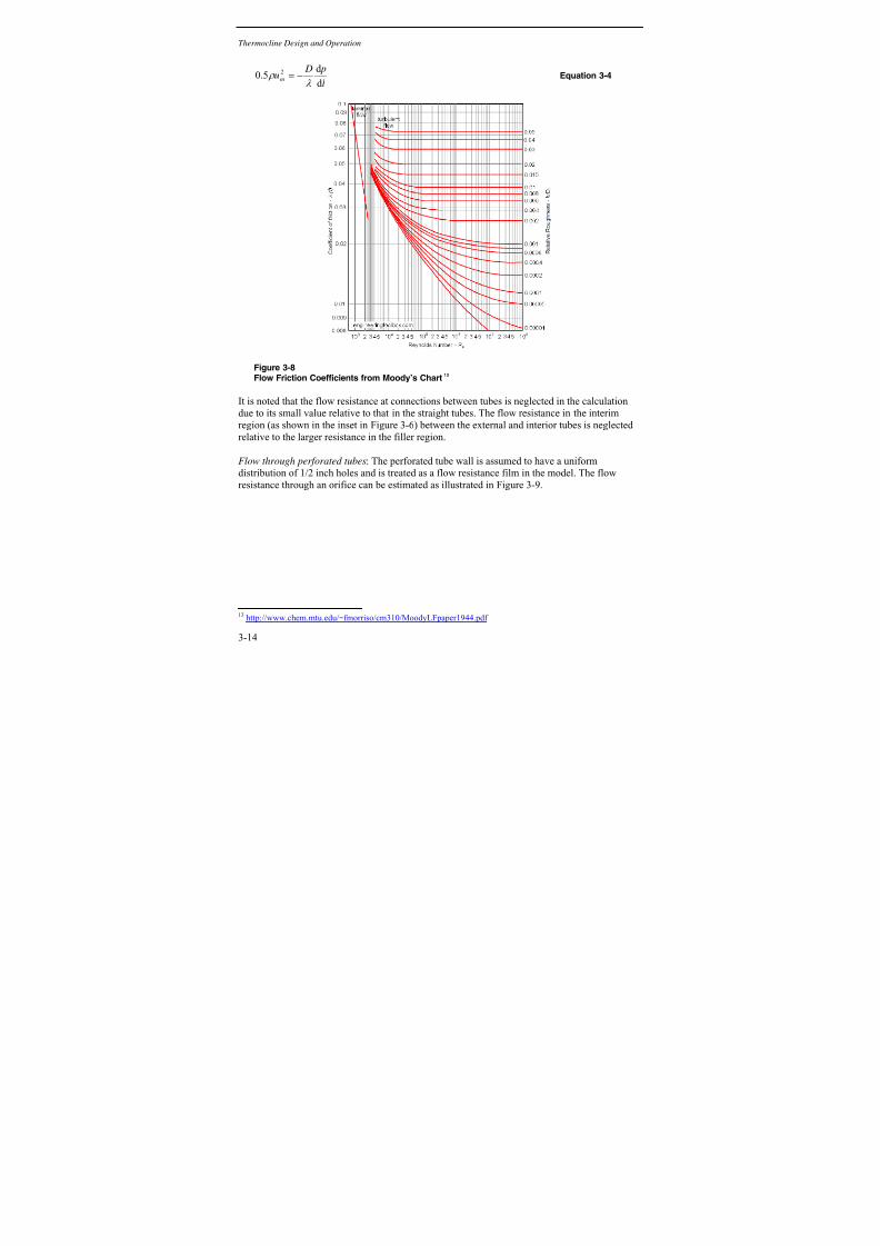
7/15/2019 Solar Storage 1019581



3-14

l

p Du

md

d 5.0 2

λ ρ −= Equation 3-4

Figure 3-8Flow Friction Coefficients from Moody’s Chart

13

It is noted that the flow resistance at connections between tubes is neglected in the calculationdue to its small value relative to that in the straight tubes. The flow resistance in the interimregion (as shown in the inset in Figure 3-6) between the external and interior tubes is neglected relative to the larger resistance in the filler region.

Flow through perforated tubes: The perforated tube wall is assumed to have a uniformdistribution of 1/2 inch holes and is treated as a flow resistance film in the model. The flowresistance through an orifice can be estimated as illustrated in Figure 3-9.

13 http://www.chem.mtu.edu/~fmorriso/cm310/MoodyLFpaper1944.pdf

7/15/2019 Solar Storage 1019581



3-15

Figure 3-9Flow through an Orifice

The relationship between flow rate and pressure difference across the orifice is given as14:

( ) ρ

π 21

4

1

2

22 2

1

1

4

p p

D

D

DQ

−

⎟⎟ ⎠

⎞⎜⎜⎝

⎛ −

= Equation 3-5

In the case of perforated feeder tubes, D2 is equivalent to the diameter of the holes in the feeder

tubes and D1 can be represented by the pitch between the holes. With the given geometries in the8 cases, the ratio between D2 and D1 is very small (≈ 0.02), and therefore, the above equationreduces to:

( ) ρ

π 21

2

2 2

4

p p DQ

−≈ Equation 3-6

Flow in the filler region: Flow in the filler region can be modeled by Darcy’s Law which isapplicable for flows in porous media at low Reynolds numbers. The typical Reynolds number inthe eight cases considered is very low (~1), and thus may be readily modeled as follows:

pK

u ∇=μ

vEquation 3-7

14 http://www.pipeflowcalculations.com/orifice/theory.htm

D2 D1

7/15/2019 Solar Storage 1019581



3-16

( )2

32

1175 ε

ε

−=

d K Equation 3-8

In Equation 3-7, uv

is velocity vector, K is permeability and μ is liquid viscosity. K is determined using Equation 3-815. The diameter of the filler particles is fixed at 1 cm in this study.

The effectiveness of the distributor is assessed based on the distribution of fluid flux over the cross section at a distance of 0.2D (D is the tank diameter) away from the distributor.Figure 3-10 through Figure 3-17 show the normalized fluid flux distribution for the differentcases. In the figures, the flux is normalized by the average value over the cross section. Asshown, the maximum flux is about 2 times the minimum, indicating that the distributor designcould be improved. Note that the velocity scales are different for each plot, as indicated by eachcolor legend.

Figure 3-10Normalized Flux Distribution over the Cross Section at a Distance 0.2D Away from theDistributor – Case 1

15 Beckermann, C., and Viskanta, R., 1988, “Natural Convection Solid/Liquid Phase Change in Porous Media,” Int.J. Heat Mass Transfer, 31, pp. 35–46.

7/15/2019 Solar Storage 1019581



3-17



7/15/2019 Solar Storage 1019581



3-18



7/15/2019 Solar Storage 1019581



3-19



7/15/2019 Solar Storage 1019581



3-20


To improve flow uniformity of the distributor, two potential options are:

1. Reduce the diameter and increase the number of orifices.

2. Use header and inlet tubes of larger diameter.

Case 8 is considered as an example: increasing the feeder diameter to 26 inches generates theflux distribution shown in Figure 3-18 below. The ratio of the maximum and minimum fluxes isnow reduced from 2 to 1.86.

Figure 3-18Normalized Flow Flux Distribution for Case 8 with Increased Feeder Diameter

7/15/2019 Solar Storage 1019581



3-21

Further investigation of the thermocline distributor manifolds with different structures wasconsidered in order to achieve a more uniform flow flux distribution inside the thermocline tank,relative to the original manifold structure.

Figure 3-19Distributor Manifold with Two Inlets

Figure 3-19 illustrates a modification of the original manifold. Two inlets are installed at thetwo opposite corners in this case. Figure 3-20 shows the normalized flow flux for Case 1 over a

cross-sectional plane that is at a distance of 0.2D from the distributor. The flow flux distributionappears symmetric, unlike that obtained earlier with only one inlet. The maximum/minimumflow flux ratio in Figure 3-20 is 1.47, which represents a significantly improved distributioncompared to the ratio of 2.23 obtained with only one inlet. This indicates that the flow fluxdistribution is more uniform with a two-inlet distributor.

7/15/2019 Solar Storage 1019581



3-22

Figure 3-20Normalized Flux Distribution over the Cross Section at a Distance 0.2D Away from theDistributor (Case 1, Two Inlets)

Another approach for improving the uniformity of flow flux distribution is to use a non-uniformdistribution of hole density (hole number per unit area) at the feeder walls. The distributor can besegregated into different sections with different hole densities, as shown in Figure 3-21. The ratioof hole number density among areas A, B, C, D, and E is 15:35:35:21:21. Areas C and B, whichare the farthest away from the inlet, have the higher densities of holes.

The resulting flow flux distribution is shown in Figure 3-22. It is clear from the figure that themaximum/minimum flow flux ratio is reduced further to 1.33 (compared to 1.47 in the two-inletdistributor case above), which indicates that the flow flux distribution is more uniform. It is possible to achieve further improvements in flow distribution uniformity if the pore number density in each area in Figure 3-21 is better-optimized.

7/15/2019 Solar Storage 1019581



3-23

Figure 3-21Non-Uniform Distribution of the ½-inch Holes on the Distributor Manifold

Figure 3-22Normalized Flux Distribution over the Cross Section at a Distance 0.2D Away from theDistributor (Case 1, Distributor in Figure 3-21)

Area A

Area B

Area CArea D

Area E

7/15/2019 Solar Storage 1019581



3-24

Surge Tanks and Molten Salt Pumps

The main function of the surge tanks (V-101 and V-102) is to provide a platform for the hot and cold molten salt pumps. The pumps are mounted in the surge tanks because the main thermoclinetank is filled with quartzite rock and sand. Although it was recommended that the molten salt pumps be placed directly inside the tank following the Solar Two project, the current projectteam chose to mount the pumps in the gravity-fed surge tanks adjacent to the main tank. Byremoving the pumps from the main thermocline tank it will not be necessary to install wells for the pumps, which will simplify the design of the thermocline tank. In addition, the surge tankswill allow the pump shafts to be significantly shorter which will have a considerable impact onthe final cost of the pumps. Next, if the pumps were housed in the thermocline tank the cold salt pipe would pass through the hot salt zone, which could significantly impact pump reliability and operation. Finally, this design simplifies pump maintenance and will allow for easier access. It isnoted that the alternative approach to embed pumps with long shafts and sleeves in the tanks mayalso be acceptable and potentially reduce costs. This may be explored further in a detailed design phase.

The surge vessels were designed with a diameter large enough to accommodate the number of pumps required for each design scenario in addition to an installed spare. The height of thevessel was selected to allow for approximately 30 seconds of residence time in the tank. Thesurge tanks are gravity fed, which means salt will flow between them only when there is adifference in liquid level. This difference is measured in liquid head (units: feet). For the flowrates reported in the heat and material balance, a 3 foot difference in head is required for the saltto flow from the surge tanks to the thermocline tank. This height difference is accomplished byraising the surge tank skirt height such that it can support a liquid level at least 3 feet above thetop of the thermocline tank. A mechanical sketch of the surge tank is presented in Appendix H.

The pumps for this process were limited to 4000 gallons per minute of throughput at any design pressure. Based on the largest commercially available pump, capacities above this limit would require multiple pumps. Using a standard design for the pump lowers the overall cost of theequipment and makes it easier to obtain replacement parts. Each pump was assumed to have avariable speed drive, and one installed spare was included in the estimates for both the hotservice and cold service to ensure reliable operation.

Heat Exchanger

For the trough design, a welded plate and frame heat exchanger was selected to accomplish theheat transfer between the salt and the circulating oil. This was chosen over a shell and tube heatexchanger due to the high duties and close temperature approaches required in each design case.

A welded plate and frame exchanger has been successfully used before in this service and is a proven design. The plate and frame heat exchanger is based on sizing from Alfa Laval, whichhas experience with heat exchangers in this service.

Additional Design Considerations

There are a number of assumptions made in this study that should be confirmed for a finaldesign.

7/15/2019 Solar Storage 1019581



3-25

1. The tank heights were selected based on a soil study performed in Barstow, California.Different locations may permit larger tanks to be constructed, which would increase theefficiency of the system and reduce costs. Conversely, building a thermocline tank in alocation with poor soil may reduce the height of the tank or increase the foundation size,either of which would increase costs.

2. Based on the operating experience at Solar One, which did not experience increased stresses on the tank from thermal ratcheting

16, the current process design does not make any

allowances for the structural impact of thermal ratcheting. Thermal ratcheting may occur over time as the packed bed is thermally cycled. As the quartzite is cooled it contracts and compacts in the bottom of the tank. When the tank is reheated the quartzite cannot returnto its original position. The quartzite then expands and places pressure on the walls of thetank. Over time this could potentially damage the tank. To eliminate risk associated withthermal ratcheting there is an R&D effort at Sandia to analyze this issue for differenttemperature spreads, size and type of aggregates used as filler, and packing density.Design considerations to minimize the impact of thermal ratcheting will be provided, if needed, to minimize the impact on the structure.

3. Depending on the exact application of the thermocline system, some of the equipment inthe scope of the estimate may be unnecessary. For example, if an existing solar plant wereretrofitted to use thermal energy storage, the main circulation pumps may already be installed as part of the existing facility. Therefore some cost savings may be achieved in the actualapplication of the thermocline system compared to the estimates presented in this study.

4. The rock and sand filler design is an important consideration. It is important to provideadequate screening and support material to separate the quartzite from the distributionmanifold. This is necessary to prevent rock and sand from exiting the thermocline tank and potentially damaging other pieces of process equipment. In addition, the quartzite has the potential to generate a significant amount of fines that may need to be filtered from the

system periodically. It may be necessary to install a filter that can be purged outside thethermocline tank. A rock only region around the distribution manifolds may help filter quartzite fines from the distribution system.

5. It may be necessary to inspect the welding on the thermocline tank periodically to check for potential corrosion damage. For this reason, provisions should be made to removesome insulation from the outside walls as necessary to inspect the bare metal surface.

6. Instead of relying on the thermocline to keep the hot and cold fluids separate, the use of insulating floaters as separators has been suggested in the literature. A floater would consistof a horizontal disk made of insulating material of an appropriate density that falls betweenthe densities of the hot and cold fluids. Active mechanisms can be used to locate and traverse

the floater within the tank and position it to yield the maximum returned energy from thestorage tank. Use of a floater, however, will rule out the use of fillers in the tank,simultaneously. NREL believes the floater option is a potentially viable, practical solution toTES that would be worth further investigation.

16 S. E. Faas, L. R. Thorne, E. A. Fuchsm and N. D. Gilbertsen,“10 MWe Solar Thermal Central Receiver PilotPlant: Thermal Storage Subsystem Evaluation Final Report.” Sandia National Laboratories: June 1986.

7/15/2019 Solar Storage 1019581



3-26

Operating Modes

Four TES operating modes are examined in this study.

In Operating Mode 1, Thermal Charging (TC), cold molten salt is removed from the bottom of the tank and heated with solar energy. The heated molten salt is then returned to the top of the

tank. There is no electricity generation. In this scenario thermal energy is stored in the tank.

In Operating Mode 2, Thermal Discharging (TD), hot molten salt is removed from the top of thetank and used to generate electricity. The cooled molten salt is then returned to the bottom of thetank. There is no thermal input in this scenario. As a result, thermal energy is being removed from the thermocline tank.

In Operating Mode 3, Thermal Regulation (TR), the system is simultaneously charging and discharging; the molten salt is heated by the solar collector field at the same time salt is beingused to generate electricity. If the solar input exceeds the power generation, thermal energy isstored. If the solar input is less than the power generation, there is a net removal of thermalenergy from the tank. For the purposes of equipment sizing it is assumed that the system has a

solar multiple of 1.8, i.e., at the design point, the solar field generates 1.8 times more thermalenergy than the energy required to operate the Rankine cycle at full load. This operating modedoes not apply to the indirect parabolic trough cases because the oil-to-salt heat exchangers onlyallow energy to be transferred in one direction at any given time. Only the direct central receiver design cases, in which the charging and discharging operations are decoupled, reference thisoperating mode.

Finally, in Operating Mode 4, Stand-by (TS), which occurs nightly or whenever the solar inputdrops below a certain level, no electricity generation takes place. In this mode a small amount of molten salt is circulated throughout the system to maintain the temperature above the freezing point of the salt. This slowly reduces the energy stored in the tank. If the molten salt in the tank

is in danger of dropping below the freezing point, all lines will be drained and the heat tracingwill be activated. Note that the lines between the thermocline tank and the surge tanks cannot bedrained. If necessary, salt can be drained to the salt melting sump.

Process Description

This section describes the general scope and operation of the TES system. The information isintended to serve as a general description of the process for both design options (trough and central power tower). Please refer to the process flow diagrams (PFDs) in Appendix B and the heat and material balances (H&MBs) in Appendix C while reading through the processdescription. Plant streams and components marked as outside battery limits (OSBL), such as

the solar field and the power block, were considered to be outside the scope of this project.The functions of each component will be explained further in the sections below.

For all of the thermocline systems, cold molten salt is added or removed from the bottom layer of the Thermocline Storage Tank (V-103), and hot molten salt is added or removed from the toplayer. Heat tracing protects the lines from freezing in the event of a no-flow scenario.

7/15/2019 Solar Storage 1019581



3-27

Indirect Parabolic Trough Design

Operating Mode 1: TC

Cold molten salt is gravity fed from the Thermocline Storage Tank (V-103) to the Cold Molten

Salt Surge Tank (V-102) at 293°C (559°F). The gravity feed allows salt to flow in either direction between the tanks, and allows cold molten salt to be added or removed from theThermocline Storage Tank (V-103) through a single nozzle. Cold molten salt is then pumped from the Cold Molten Salt Surge Tank (V-102) to either the Oil/Molten Salt Exchanger (E-101)or the Thermocline Storage Tank (V-103) using the Cold Molten Salt Pump (P-102).

The Oil/Molten Salt Exchanger (E-101) is a plate heat exchanger that transfers energy betweenthe molten salt and hot circulating oil. The flow rate of molten salt through the exchanger isadjusted by flow control to maintain the outlet salt temperature at 400°C (752°F). Flow control isaccomplished by manipulating the variable speed drive of the Cold Molten Salt Pump.

Hot oil is supplied to the heat exchanger by the parabolic trough field (OSBL) to heat the cold molten salt. The cooled oil is then returned to the trough field (OSBL) for reheating. The hot saltis then returned to the Thermocline Storage Tank (V-103).

Operating Mode 2: TD

Hot molten salt is gravity fed from the Thermocline Storage Tank (V-103) to the Hot Molten SaltSurge Tank (V-101) at 400°C (752°F). The surge tank and thermocline liquid levels aremaintained near the same elevation because the tanks are connected with an open pipe. Thegravity feed allows salt to flow in either direction between the tanks. The hot molten salt is then pumped from the Hot Molten Salt Surge Tank (V-101) to either the Oil/Molten Salt Exchanger (E-101) or the Thermocline Storage Tank (V-103).

In the heat exchanger, the hot molten salt is cooled by the Therminol oil returning from thePower Generation Facility (OSBL). The flow rate of molten salt through the exchanger isadjusted by flow control to maintain the outlet salt temperature at 293°C (559°F). Flow control isaccomplished by a variable speed drive set on the Hot Molten Salt Pump (P-101).

Cool molten salt from the Oil/Molten Salt Exchanger (E-101) is returned to the ThermoclineStorage Tank (V-103). The oil heated in the heat exchanger is then returned to the Power Generation Facility to produce electricity (OSBL).

Operating Mode 4: TS

In Operating Mode 4, a small amount of molten salt will circulate throughout the TES systemusing both the hot and cold molten salt pumps. Thermal oil circulating pumps will be maintained at low flow. This is done to maintain the temperatures above the minimum for both the TESsystem and the HTF oil loop to prevent freezing. If the salt temperature approaches the freezing point, flow will be stopped and all lines will be allowed to drain back to the thermocline tank.

7/15/2019 Solar Storage 1019581



3-28

Heat tracing will then be used to maintain the temperatures of both the molten salt and Therminol oil systems.

Direct Central Receiver Design

Operating Mode 1: TC

In this mode cold molten salt is gravity fed from the Thermocline Storage Tank (V-103) to theCold Molten Salt Surge Tank (V-102) at 293°C (559°F). The gravity feed allows salt to flow ineither direction between the tanks, and allows cold molten salt to be added or removed from theThermocline Storage Tank (V-103) through a single nozzle. Cold molten salt is then pumped from the Cold Molten Salt Surge Tank (V-102) to the Central Power Tower (OSBL) with theCold Molten Salt Pump (P-101).

In the central power tower, solar energy is used to heat the molten salt from 293°C (559°F) to

560°C (1040°F). This temperature is maintained through flow control of the molten salt. Flowcontrol is accomplished using a variable speed drive on the Cold Molten Salt Pump (P-102). Hotsalt from the Central Power Tower (OSBL) is returned to the Thermocline Storage Tank (V-103) by gravity flow.

Operating Mode 2: TD

In this mode hot molten salt is gravity fed from the Thermocline Storage Tank (V-103) to theHot Molten Salt Surge Tank (V-101) at 560°C (1040°F). The gravity feed allows salt to flow ineither direction between the tanks, and allows salt to be added or removed from the ThermoclineStorage Tank (V-103) through a single nozzle. Hot molten salt is then pumped from the Hot

Molten Salt Surge Tank (V-102) to the Power Generation Facility (OSBL) using the Hot MoltenSalt Pump (P-101).

At the Power Generation Facility thermal energy will be removed from the molten salt, cooling itdown to the minimum defined TES operating cut-off temperature (See Chapter 5). Thistemperature is maintained through flow control of the salt. This flow control is accomplished using a variable speed drive on the Hot Molten Salt Pump (P-101). Cold salt from the Power Generation Facility (OSBL) is returned to the Thermocline Storage Tank (V-103) by gravityflow.

Operating Mode 3: TRIn Operating Mode 3 there are two molten salt circulation loops. In the first loop cold salt isremoved from the bottom of the Thermocline Storage Tank (V-103) at 293°C (559°F) and pumped to the Central Power Tower (OSBL). The salt is then heated to 560°C (1040°F) and returned to the top of the thermocline tank. This loop is the same as Operating Mode 1, and isdescribed in detail above.

7/15/2019 Solar Storage 1019581



3-29

In the second molten salt loop, hot salt is removed from the top of the tank at 560°C (1040°F)and pumped to the Power Generation Facility (OSBL). At the Power Generation Facility the saltis cooled to 293°C (559°F) and returned to the bottom of the thermocline tank. This loop is thesame as Operating Mode 2, which is described above.

If the flow rate of molten salt through the receiver is greater than the flow rate of molten salt

through the power cycle loop, the thermocline boundary layer in the tank will descend as hotmolten salt occupies a larger fraction of the tank. If the flow rate of the power cycle loop isgreater than the flow rate through the receiver, the thermocline boundary layer in the tank willascend. In the event that both flow rates are equal, the thermocline zone will remain at a constantlevel. Heat tracing is used to ensure that the lines will not freeze in a no-flow condition.

The temperature control of the hot molten salt and the cold molten salt is accomplished by flowcontrol. This is done through the use of variable speed drives on the Hot and Cold Molten SaltPumps. The flow rate of the cold molten salt is adjusted to provide hot molten salt at 560°C(1040°F). This flow rate varies depending on the available solar thermal energy. The flow rate of the hot molten salt is adjusted to provide cold molten salt at 293°C (559°F). The flow rate of this

stream is determined by the required power generation.

Operating Mode 4: TS

In Operating Mode 4 a small amount of molten salt will be circulated throughout the systemusing both the hot and cold molten salt pumps. This is done to maintain the temperature of thesystem. If the salt temperature approaches the freezing point, flow will be stopped and all lineswill be allowed to drain back to the thermocline tank. Heat tracing will then be used to maintainthe temperature of the system.

Preheating the Thermocline

Due to the high temperature of the salt system, it is necessary to preheat the thermocline tank before molten salt is added. The preheating system is designed to raise the temperature of thequartzite bed and the tank shell to 288°C (550°F), which is above the melting point of the salt.This is to both prevent damage to the tank from thermal stress, and to ensure that the salt doesnot freeze on any cold spots during the initial fill. The preheating system defined consists of arotary blower and a fired heater. The blower moves air through the heater and raises thetemperature to 315°C (599°F). The equipment is sized to heat the tank to 288°C (550°F) over a period of 30 days. This temperature was chosen because it is 50°C above the freezing point of the salt, which should provide adequate safety margin. This time period was chosen to ensurethat thermal stresses would not damage the tank or the packing, and also to minimize the size

of the temporary equipment. The tank also has electric heat tracing.

Charging the System with Salt

To introduce salt into the system, solid salt will be added to the Salt Melting Sump (V-104). TheSalt Melting Sump is a small carbon steel tank with an immersion heater (E-102, Salt MeltingHeater) and a Salt Charging Pump (P-103). The system has been sized in all design cases to melt

7/15/2019 Solar Storage 1019581



3-30

all of the salt for the system in 30 days. After the thermocline system has begun operation, theequipment will be used as necessary to add any makeup salt to the system. In the event of asystem upset, provisions have been included to drain salt to the sump as necessary.

Thermocline Tank Efficiencies

As mentioned above, the thermocline tank design was based on the Purdue methodology11

. Thetank sizing relative to two-tank systems was determined using the efficiency calculations below.The tank efficiency is defined in Equation 3-3, and is roughly a measure of how much of the tank volume is lost in the tank to maintaining the thermocline boundary. The thermocline tank efficiencies for the 95% threshold (threshold temperatures are 395°C and 547°C for trough and central receiver, respectively) are given in Table 3-9. The efficiencies of the two-tank system areassumed to be 100%. The thermal losses17 constitute energy lost to the atmosphere through thetank insulation. These losses are the same for both the thermocline tank and an equivalent state-of-the-art two-tank system. They include the thermal energy storage system only, and do notinclude energy lost in electricity generation.

Table 3-9Molten Salt Thermocline Storage Tank Estimated Thermal Efficiencies

Design Case MWht

Maximum TESTemperature

TechnologyTank

EfficienciesThermalLosses

1 400°C (752°F) Indirect Trough 89% 0.40%

2100

560°C (1040 °F) Direct Central Receiver 89% 0.38%


4500

560°C (1040 °F) Direct Central Receiver 89% 0.10%


61000

560°C(1040 °F) Direct Central Receiver 89% 0.06%


83000

560°C (1040 °F) Indirect Trough 89% 0.07%

Note: Design tank efficiencies estimated by Black & Veatch were determined to be conservative by roughly15%. This additional design margin effectively accounts for the lack of uniform distribution, wall effects, as- built void coefficient, filler, and as-built height. The result is an extension of the discharge time by over an hour and increased energy extraction from the thermocline tank.

It can be seen from the definition of tank efficiency that η95 is a function of both the Reynolds

number and the tank height. In the above design cases the tank height is always set at 40 feet(except for Case 8, where the tank height is 47 feet). This means that the Reynolds number is theonly variable in the efficiency calculation. The Reynolds number is defined as:

17 Yang, Z., Garimella, S.V. Molten-salt Thermal Energy Storage in Thermoclines under Different EnvironmentalBoundary Conditions. Applied Energy (2010), doi:10.1016/j.apenergy.2010.04.024.

7/15/2019 Solar Storage 1019581



3-31

c

d u

ν

⋅=Re Equation 3-9

Where u is the salt flow rate, d is the diameter of the filler, and νc is the viscosity of the fluid atthe cold inlet temperature.

7/15/2019 Solar Storage 1019581


7/15/2019 Solar Storage 1019581


4-1

4 CAPITAL COST ESTIMATES

The cost estimates indicate that the proposed thermocline thermal energy storage system hasthe potential to significantly reduce TES costs compared to a two-tank storage system. There is awide cost range that depends largely on the scale of the project and the operating temperature.The cost estimates developed in this study include both direct and indirect costs with acontingency of 15% and sales tax. They are presented in January 2010 dollars. A complete breakdown of the equipment and engineering costs is provided in Appendix G. A summaryof the total installed capital costs is provided in Table 4-1.

Table 4-1 Molten Salt Thermocline Storage Capital Costs

Storage Capacity(MWht)

TechnologyMaximum TESTemperature

ThermoclineCost ($)

Cost Per UnitCapacity($/kWht)

Indirect Trough 400°C (752°F) 24,613,000 246100

Direct Central Receiver 560°C (1040 °F) 13,184,000 132






Direct Central Receiver 560°C (1040 °F) 66,000,000* 44*



Indirect Trough 400°C (752°F) 254,333,333* 73*3500


* Values were interpolated or extrapolated from other design case results.

For comparison, estimates were prepared for an equivalent set of two-tank thermal energystorage systems. These estimates are provided in Table 4-2. Both sets of quotes provided inTable 4-1 and Table 4-2 have an uncertainty of approximately +40%/-20% in accordance withAACE Class 4 estimate. The uncertainty with these estimates can be reduced with additionaldesign or demonstration of the concepts identified in this report. Detailed modeling, design or demonstration of the following items will likely be necessary to confirm the conceptual designs presented here:

7/15/2019 Solar Storage 1019581


Capital Cost Estimates

4-2

• Dynamic modeling of thermocline

• Thermal ratcheting

• Tank materials

• Distributor design

• Other tank internals, including structural supports

Table 4-2 Two-Tank Molten Salt Thermal Storage Capital Costs

Storage Capacity(MWht)


Two-Tank Cost ($)

Cost Per UnitCapacity($/kWht)














It can be seen from this information that the thermocline system offers the lowest installed capital cost at each design capacity. The average savings for the thermocline system isapproximately $25 per kWht, which is an average reduction of 24%. For the largest single-tank designs, the savings were 37% for the indirect trough 1500 MWht case and 33% for the directcentral receiver 3500 MWht case. It can also be seen that the direct TES systems are less

expensive than indirect thermal energy storage due to the higher charging temperatures, whichminimizes the required storage volume. This information is presented graphically in Figure 4-1.

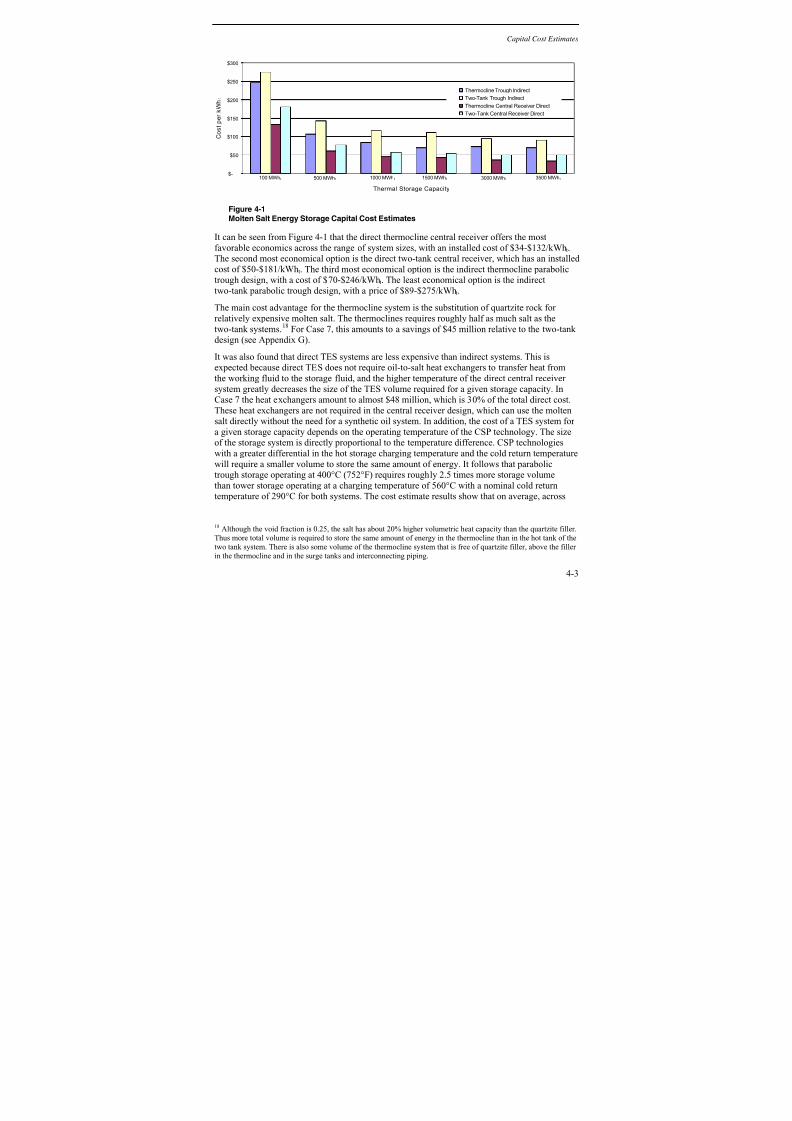
7/15/2019 Solar Storage 1019581



4-3

$-

$50

$100

$150

$200

$250

$300


C o s t p e

r k W h t






Figure 4-1 Molten Salt Energy Storage Capital Cost Estimates

It can be seen from Figure 4-1 that the direct thermocline central receiver offers the mostfavorable economics across the range of system sizes, with an installed cost of $34-$132/kWht.The second most economical option is the direct two-tank central receiver, which has an installed cost of $50-$181/kWht. The third most economical option is the indirect thermocline parabolictrough design, with a cost of $70-$246/kWht. The least economical option is the indirecttwo-tank parabolic trough design, with a price of $89-$275/kWht.

The main cost advantage for the thermocline system is the substitution of quartzite rock for relatively expensive molten salt. The thermoclines requires roughly half as much salt as thetwo-tank systems.

18For Case 7, this amounts to a savings of $45 million relative to the two-tank

design (see Appendix G).

It was also found that direct TES systems are less expensive than indirect systems. This isexpected because direct TES does not require oil-to-salt heat exchangers to transfer heat fromthe working fluid to the storage fluid, and the higher temperature of the direct central receiver system greatly decreases the size of the TES volume required for a given storage capacity. InCase 7 the heat exchangers amount to almost $48 million, which is 30% of the total direct cost.These heat exchangers are not required in the central receiver design, which can use the moltensalt directly without the need for a synthetic oil system. In addition, the cost of a TES system for a given storage capacity depends on the operating temperature of the CSP technology. The sizeof the storage system is directly proportional to the temperature difference. CSP technologieswith a greater differential in the hot storage charging temperature and the cold return temperaturewill require a smaller volume to store the same amount of energy. It follows that parabolic

trough storage operating at 400°C (752°F) requires roughly 2.5 times more storage volumethan tower storage operating at a charging temperature of 560°C with a nominal cold returntemperature of 290°C for both systems. The cost estimate results show that on average, across

18 Although the void fraction is 0.25, the salt has about 20% higher volumetric heat capacity than the quartzite filler.Thus more total volume is required to store the same amount of energy in the thermocline than in the hot tank of thetwo tank system. There is also some volume of the thermocline system that is free of quartzite filler, above the filler in the thermocline and in the surge tanks and interconnecting piping.

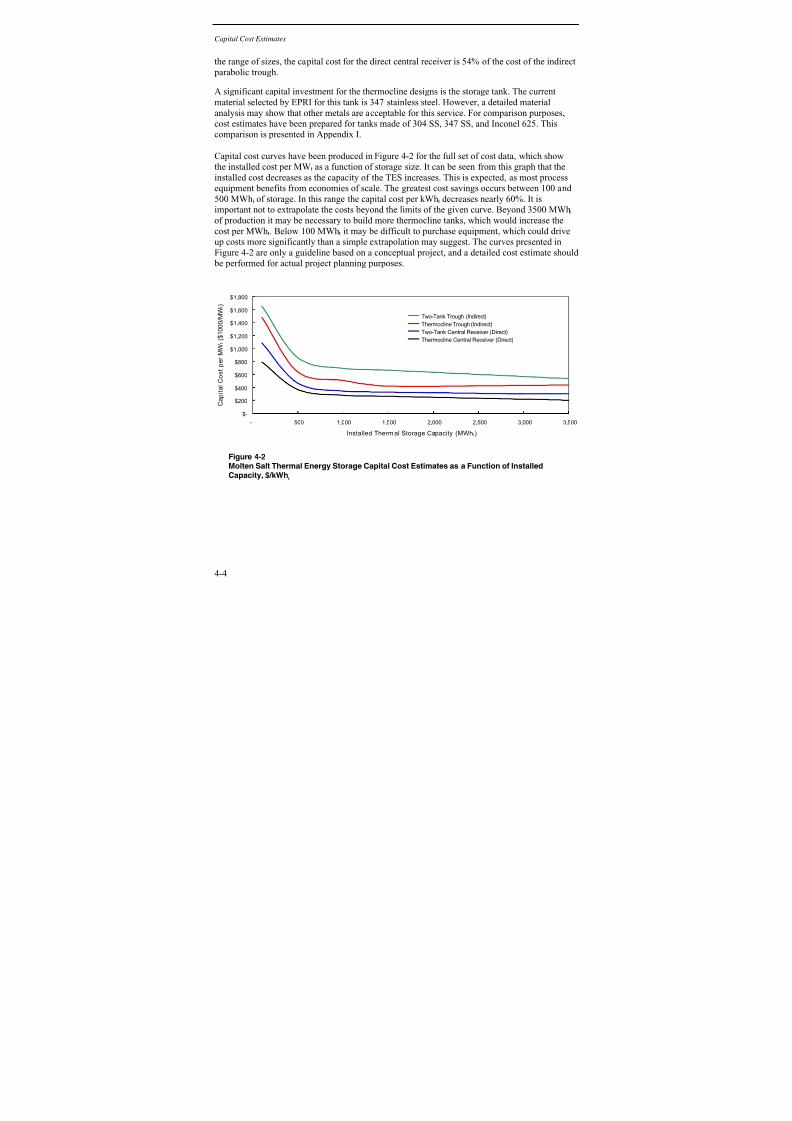
7/15/2019 Solar Storage 1019581



4-4

the range of sizes, the capital cost for the direct central receiver is 54% of the cost of the indirect parabolic trough.

A significant capital investment for the thermocline designs is the storage tank. The currentmaterial selected by EPRI for this tank is 347 stainless steel. However, a detailed materialanalysis may show that other metals are acceptable for this service. For comparison purposes,cost estimates have been prepared for tanks made of 304 SS, 347 SS, and Inconel 625. Thiscomparison is presented in Appendix I.

Capital cost curves have been produced in Figure 4-2 for the full set of cost data, which showthe installed cost per MWt as a function of storage size. It can be seen from this graph that theinstalled cost decreases as the capacity of the TES increases. This is expected, as most processequipment benefits from economies of scale. The greatest cost savings occurs between 100 and 500 MWht of storage. In this range the capital cost per kWht decreases nearly 60%. It isimportant not to extrapolate the costs beyond the limits of the given curve. Beyond 3500 MWht of production it may be necessary to build more thermocline tanks, which would increase thecost per MWht. Below 100 MWht it may be difficult to purchase equipment, which could driveup costs more significantly than a simple extrapolation may suggest. The curves presented inFigure 4-2 are only a guideline based on a conceptual project, and a detailed cost estimate should be performed for actual project planning purposes.

$-

$200

$400

$600

$800

$1,000

$1,200

$1,400

$1,600

$1,800

- 500 1,000 1,500 2,000 2,500 3,000 3,500

Installed Therm al Storage Capacity (MWht)

C a p i t a l C o s t p e r M W t ( $ 1 0 0 0 / M W t )

Two-Tank Trough (Indirect)

Thermocline Trough (Indirect)

Two-Tank Central Receiver (Direct)

Thermocline Central Receiver (Direct)

Figure 4-2 Molten Salt Thermal Energy Storage Capital Cost Estimates as a Function of Installed

Capacity, $/kWht

7/15/2019 Solar Storage 1019581


5-1

5 PERFORMANCE ANALYSIS

In conjunction with the structural design study conducted by Black & Veatch, the performanceof a thermocline TES system was analyzed by Sandia National Laboratories, the NationalRenewable Energy Laboratory (NREL), and Purdue University. These analyses investigated theannual performance of a thermocline system compared to a two-tank system, the thermal performance of the thermocline with regards to thermal gradients and natural convection duringdwell periods, and the distributor manifold performance.

Annual Performance

The analysis performed by Sandia compared the annual performance of a thermocline systemwith that of a two-tank TES design for a parabolic trough power plant. The two-tank systemrepresents today’s baseline technology as demonstrated at the 50 MWe Andasol plant nowoperating in Spain. With a solar multiple of ~2, the excess collector field energy at Andasol isstored within a two-tank molten-salt system for later use by the steam turbine. A simplified schematic and some key design parameters19

for this two-tank system are shown in Figure 5-1 and Table 5-1.

Figure 5-1Schematic of Andasol-Type Parabolic Trough Plant

19 Relloso, Sergio and Yolanda Gutierrez, “Real Application of Molten Salt Thermal Storage to Obtain HighCapacity Factors in Parabolic Trough Plants,” SENER, SolarPACES 2008, Las Vegas, NV

7/15/2019 Solar Storage 1019581


Performance Analysis

5-2

Table 5-1Key Design Parameters for Andasol-Type Parabolic Trough Plant

Turbine Capacity (gross) 50 MWe

Turbine Efficiency (Full Power) 37%

Storage Thermal Rating 1010 MWht, 7.4 hrs

Storage Tank Size*, H x D 2 tanks, 14 m x 37 m each

Storage Fluid Solar salt (60% NaNO3, 40% KNO3)

Storage Heat Exchanger 16,000 m2

Solar Collector Field Aperture Area 510,000 m2

Solar Collector Assembly, W x L 5.77 m x 148 m

Solar Collector Row Spacing 16.2 m

Solar Collector Fluid (HTF) Therminol VP-1

*It was observed that the Black & Veatch tank design volume for 1000 MWht is approximately13% lower than the reported volume of the Andasol system. This may be a result of severalfactors, such as slightly lower capacity (1000 MWht vs. 1010 MWht), tank heel level, head space, turbine efficiency used to determine hours of storage, etc.

TRNSYS 16 was used to simulate the annual perfor mance of this two-tank plant. A combinationof standard-TRNSYS components, STEC-TRNSYS

20components, and some new system-

control components were used to create the model. The logic model is depicted in Figure 5-2 and Figure 5-3 and the important model parameters are listed in Table 5-1 and Table 5-2.

20 STEC components can be downloaded from http://sel.me.wisc.edu/trnsys/trnlib/stec/stec.htm

7/15/2019 Solar Storage 1019581



5-3

Figure 5-2TRNSYS Model of Andasol-Type Power Plant

Figure 5-3Expanded TRNSYS Two-Tank Macro

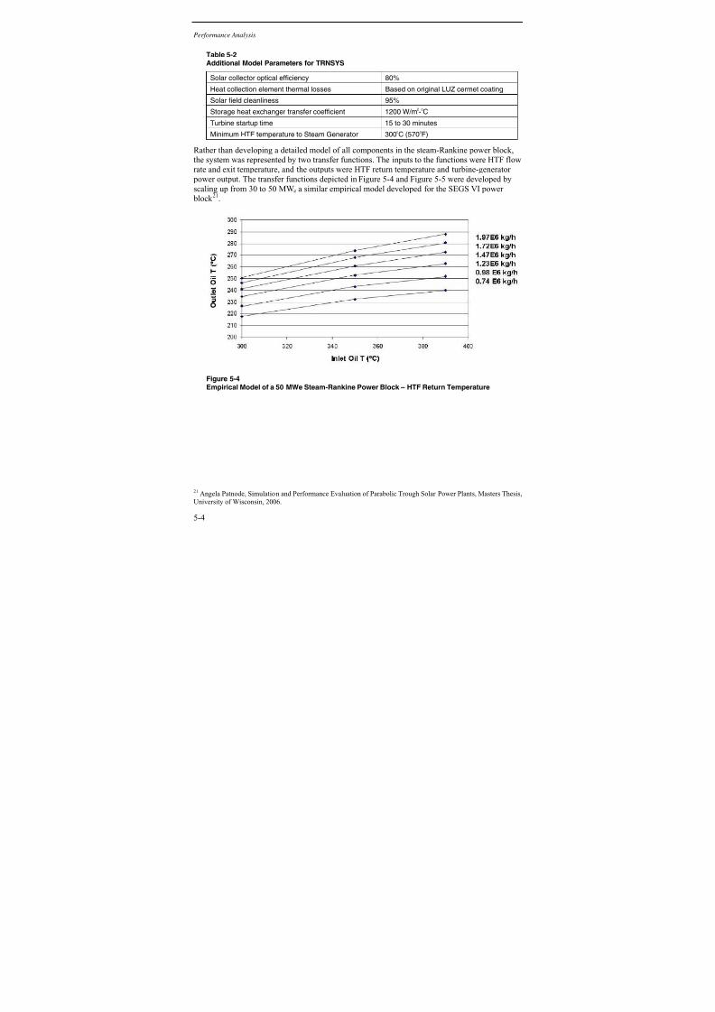
7/15/2019 Solar Storage 1019581



5-4

Table 5-2Additional Model Parameters for TRNSYS

Solar collector optical efficiency 80%

Heat collection element thermal losses Based on original LUZ cermet coating

Solar field cleanliness 95%

Storage heat exchanger transfer coefficient 1200 W/m2-

oC

Turbine startup time 15 to 30 minutes

Minimum HTF temperature to Steam Generator 300oC (570

oF)

Rather than developing a detailed model of all components in the steam-Rankine power block,the system was represented by two transfer functions. The inputs to the functions were HTF flowrate and exit temperature, and the outputs were HTF return temperature and turbine-generator power output. The transfer functions depicted in Figure 5-4 and Figure 5-5 were developed byscaling up from 30 to 50 MWe a similar empirical model developed for the SEGS VI power block 21.

Figure 5-4Empirical Model of a 50 MWe Steam-Rankine Power Block – HTF Return Temperature

21 Angela Patnode, Simulation and Performance Evaluation of Parabolic Trough Solar Power Plants, Masters Thesis,University of Wisconsin, 2006.

7/15/2019 Solar Storage 1019581



5-5

Figure 5-5Empirical Model of a 50 MWe Steam-Rankine Power Block – Turbine Generator Output

The minimum oil-inlet temperature to the steam generator is shown in Figure 5-5 to be 300°C(570°F). This is based on actual experience at SEGS VI; near noontime in the winter, the field outlet temperature is dropped from the design value of 390°C (734°F) to ~300°C (570°F) and theRankine cycle temperature and pressure is dropped to maintain 50°C of superheat (called sliding pressure operation). The Kramer Junction plant staff and Sandia’s evaluation have found thatthis operating approach maximizes the overall solar-to-electric efficiency.22 Establishing theminimum oil operating temperature is very important to evaluation of thermocline storage, asdescribed later.

The two-tank TRNSYS model was run using a three-minute time step and the hourly TMY filefor Tucumcari, New Mexico. This weather file was chosen because the annual DNI is similar tosouthern Spain, i.e., 2.3 MWh/m2-yr. The model predicted an annual gross electricity output of 152 GWh. This value is similar to values predicted for Andasol prior to plant startup 23,indicating that the model’s results are reasonable.

The next step in the analysis was to replace the two-tank model with a thermocline model. Thethermocline chosen for this study is Case 5 defined by Black and Veatch, in Chapter 3: a 1000MWht thermocline with a height of 12.2 m (40 ft) and a diameter of 46.3 m (152 ft). A simplified schematic is shown in Figure 5-6.

22 Lippke, Frank, Simulation of the Part-Load Behavior of a 30 MWe SEGS Plant, SAND95-1293, June 1995. Thisreport also describes the basis for the STEC Type 197 trough model.23 Geyer, et. al., “Dispatchable Solar Electricity for Summerly Peak Loads from the Solar Thermal Projects Andasol1 Y Andasol 2 (sic),” Solar Millennium, SolarPACES 2006, Seville, Spain. The paper quotes 3589 full load hourswith 12% from fossil. Thus, solar-only performance = 0.88*49.9 MWe*3589 = 157.6 GWh.

7/15/2019 Solar Storage 1019581



5-6

Figure 5-6Andasol-Type Plant with 1000 MWht Thermocline Storage System

The TRNSYS logic model for this plant is depicted in Figure 5-7. Only the storage portion of the model is shown since the remainder is the same as the two-tank model. The void fraction of the tank is assumed to be 24% based on experience at the Solar One thermocline tank. This is

comparable to the 25% void fraction assumed in the Black & Veatch design. The density of the rock is 1940 kg/m3

and the specific heat is 880 J/kg-C. The basis of the thermocline tank model was the STEC Type 502, which was developed for SolarPACES a few years ago and is avariation of the standard TRNSYS Type 10 component. The tank is divided into several equally-sized control volumes (23 stacked cylinders used here) and a first-order differential equationdescribes the energy balance of each cylinder.

7/15/2019 Solar Storage 1019581



5-7

Figure 5-7TRNSYS Model of Thermocline Storage System

The thermocline TRNSYS model was run using the same time step and the hourly TMY file as

for the two-tank system. The model predicted an annual gross electricity output of 153 GWh.This value is virtually identical to the two-tank plant, which suggests that it should be possible to

develop a thermocline system that achieves the same overall power plant performance as atwo-tank system.

Previous investigators of thermoclines have assumed that thermocline exit temperatures

must remain high to produce useful electricity. As discussed previously, the SEGS VI power

block is designed to operate up to 90°C below the design value, i.e., 300°C (570°F) vs. 390°C(734°F). Thermocline plants would not perform as well as a two-tank plant if the degradation in

temperature was not allowed. To estimate the effect, the TRNSYS models were rerun assuming a

minimum temperature of 340°C (644°F) and 360°C (680°F). The results of this investigation are

shown in Table 5-3.

Table 5-3Comparison of Minimum Temperature Limitation Results

Min Oil T to Power Block 2-Tank Plant Electricity Themocline Plant Electricity

300o

C 152 GWh 149 GWh

340o

C 149 GWh 135 GWh

360o

C 146 GWh 125 GWh

7/15/2019 Solar Storage 1019581



5-8

Thermal Performance

The thermal performance of the thermocline systems was evaluated by both NREL and PurdueUniversity. While the solid fill used within a thermocline tank helps to lower the overall cost of the TES by reducing the amount of relatively expensive molten salt required, the presence of

solids in the tank can cause the temperature gradients at the hot/cold salt interface to spread outmore than in the absence of solids. This spreading reduces the effective capacity of the tank. Toassess its behavior and the overall thermal cycling efficiency of the TES, it is necessary to modelthe thermal/hydraulic mechanisms that occur in the thermocline tank.

NREL Analysis

The thermocline system analyzed by NREL was modeled in two separate steps by first modelingthe core of the tank and then analyzing its wall regions. The core region has adiabatic boundaryconditions, whereas the wall region’s external wall loses heat to the environment.

The core region model should be applicable to tanks of all sizes (diameters). As per Black &Veatch, the largest tank feasible for TES is estimated to be about 15.2 m (50 ft) in height and about 48.8 m (160 ft) in diameter. This size represents a volumetric capacity of about 28,400 m3

(over 7 million gallons). Based on their assumed temperature difference of 107°C, such a tank represents a storage capacity of about 1500 MWht or a power generation capacity of about 85MWe over a 6-hour period.

The NREL model used solid fillers shaped in a structurally regular manner to eliminate lateralstructural loads to the side walls of the tank. The selected structural solid fills were in the form of hexagonal rods or a honeycomb-like structure that spans the entire height of the tank (Note: thisdesign was not consistent with the Black & Veatch design analysis; capital costs were based on a

quartzite rock/sand mixture). The void fraction, denoted by α, is filled by the molten salt.

Table 5-4 summarizes the key assumptions made for the numerical model.

7/15/2019 Solar Storage 1019581



5-9

Table 5-4Modeling Assumptions

Quantity Value Units Remarks

Hot salt temperature 385 (°C)

Cold salt temperature 300 (°C)

Tank void fraction α (---) Variable (between 0 and 1)

Tank height 14 (m)

Tank discharge time 6*3600 (s)

Molten salt velocity 0.648/ α (mm/s) Varies with tank void fraction

For a nominal 600 MWt tank, Figure 5-8 shows the variation of the required tank volume,equivalent density of the fluid/filler mixture and the fluid residence time, as functions of the tank

void fraction, α. When α=1, the tank contains fluid only, and when α=0, it is all solid.

Due to the higher density of the solid fill, the bulk density of the mixture increases withdecreasing α. The solid also has a lower specific heat capacity than the fluid. Therefore,increasing the amount of solid increases the required tank volume.

Also plotted in this figure is the fluid residence or breakthrough time, which represents the timeto replace the tank fluid once. At a residence time of 6 hours the tank is completely filled with

only fluid (α=1). As more solid is introduced, the void fraction decreases, and the fluid is forced to move through the tank more rapidly, resulting in decreased residence times. For example, theresidence time for the fluid is only 1.5 hours when the tank has a void fraction of 0.25. These

results hold true for all size tanks. Increased thermal capacity for the tank will increase itsvolume proportionately.

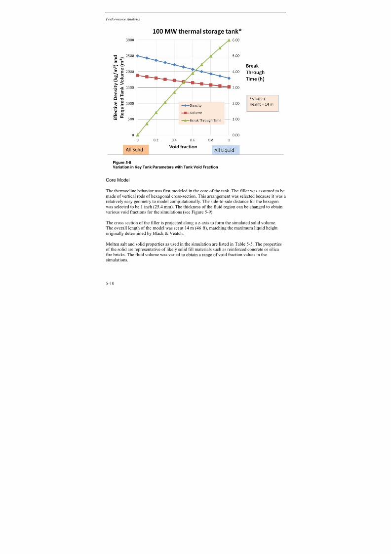
7/15/2019 Solar Storage 1019581



5-10

Figure 5-8Variation in Key Tank Parameters with Tank Void Fraction

Core Model

The thermocline behavior was first modeled in the core of the tank. The filler was assumed to bemade of vertical rods of hexagonal cross-section. This arrangement was selected because it was arelatively easy geometry to model computationally. The side-to-side distance for the hexagonwas selected to be 1 inch (25.4 mm). The thickness of the fluid region can be changed to obtainvarious void fractions for the simulations (see Figure 5-9).

The cross section of the filler is projected along a z-axis to form the simulated solid volume.The overall length of the model was set at 14 m (46 ft), matching the maximum liquid height

originally determined by Black & Veatch.

Molten salt and solid properties as used in the simulation are listed in Table 5-5. The propertiesof the solid are representative of likely solid fill materials such as reinforced concrete or silicafire bricks. The fluid volume was varied to obtain a range of void fraction values in thesimulations.

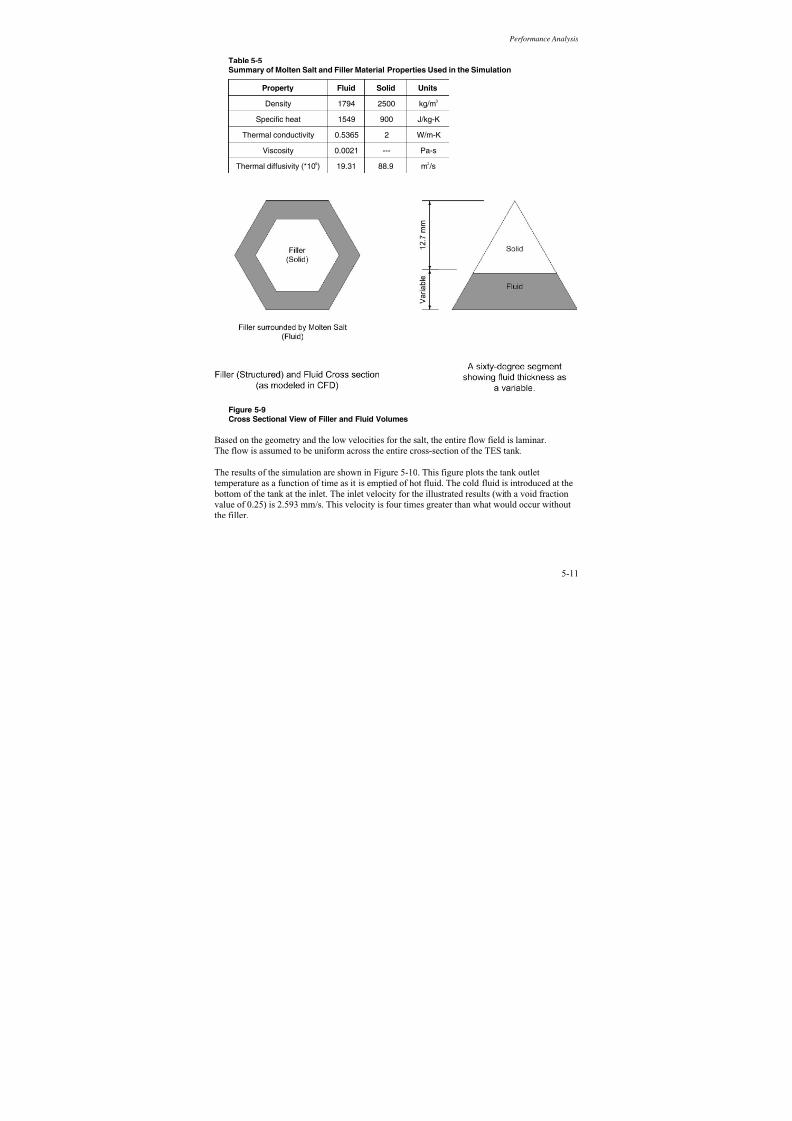
7/15/2019 Solar Storage 1019581



5-11

Table 5-5Summary of Molten Salt and Filler Material Properties Used in the Simulation

Property Fluid Solid Units

Density 1794 2500 kg/m3

Specific heat 1549 900 J/kg-K

Thermal conductivity 0.5365 2 W/m-K

Viscosity 0.0021 --- Pa-s

Thermal diffusivity (*106) 19.31 88.9 m

2 /s

Figure 5-9Cross Sectional View of Filler and Fluid Volumes

Based on the geometry and the low velocities for the salt, the entire flow field is laminar.The flow is assumed to be uniform across the entire cross-section of the TES tank.

The results of the simulation are shown in Figure 5-10. This figure plots the tank outlettemperature as a function of time as it is emptied of hot fluid. The cold fluid is introduced at the bottom of the tank at the inlet. The inlet velocity for the illustrated results (with a void fractionvalue of 0.25) is 2.593 mm/s. This velocity is four times greater than what would occur withoutthe filler.

7/15/2019 Solar Storage 1019581



5-12

Two temperatures are plotted as a function of time over 8 hours. The outlet temperature of thefluid exiting the thermocline tank is indicated using red squares for the simulation. An averagesolid filler temperature is indicated using blue diamonds. The elapsed time is indicated on thex-axis in minutes. All temperatures are normalized using the temperature difference between themaximum and minimum temperatures, as indicated below:

The temperature of the outlet fluid, τfo, is normalized as:

minmax

min fo fo

T T

T T

−

−=τ Equation 5-1

and the solid average temperature is normalized as:

minmax

minsasa

T T

T T

−

−=τ Equation 5-2

where, Τsa is the average solid temperature. Τmax and Τmin are 385°C (725°F) and 300°C (570°F),respectively, as listed in Table 5-4.

From this figure, it can be seen that the average solid temperature decreases mostly linearly,except at the tail end when the entire solid has cooled to the incoming fluid temperature. Thefluid outlet temperature remains constant for up to 4.5 hours and then begins to drop off gradually.

7/15/2019 Solar Storage 1019581



5-13

Figure 5-10Variation of Fluid Outlet and Solid Average (Non-dimensional) Temperatures as Functionsof Elapsed Time (Minutes)

The drop-off in the outlet temperature is the result of the spread of the thermocline interface between hot and cold fluids. In simple one-dimensional conduction, partial differential equationsfor thermal diffusion lead to a temperature distribution that is fully represented by an error function24.

The approximation for the error function follows the form:

( )⎪⎭

⎪⎬⎫

⎪⎩

⎪⎨⎧

⎟⎟

⎠

⎞⎜⎜⎝

⎛ −−=

π

241

xexpsqrt xerf Equation 5-3

24 The error function, normally denoted as erf(x) is defined as ( ) ∫ −= x

dx xe xerf 0

.2

In this case, for ease of

evaluation, this function was approximated as: ( )⎪⎭

⎪⎬⎫

⎪⎩

⎪⎨⎧

⎟⎟

⎠

⎞⎜⎜⎝

⎛ −−=

π

241

xexpsqrt xerf . See Oona’s approximation

provided by S. Kalkaja. This approximation differs from its actual value by less than 0.8%.

7/15/2019 Solar Storage 1019581



5-14

The fluid outlet temperature is expressed as:

( ){ }δ τ erf fo −= 1 Equation 5-4

where δ is a non-dimensional time, based on the time for breakthrough, defined as:

s

dyr

t

t t t −−=δ ) sdyr t / t t t −−=δ Equation 5-5

Here, three time parameters are indicated, and all times are represented in seconds.

t r is the residence time for the fluid, or the tank height divided by the actual fluid verticalabsolute velocity.

t dy is a delay caused by the heat transfer that occurs between the solid and the liquid.

t s represents the inverse of the slope of the decline in temperature versus time, which indicatesthe spread of the thermocline region.

Using these parameters, a fit for the variation of fluid outlet temperature versus time was found and is shown in the figure by the green line. For this fit, the “time” parameters were found to be:

.st and ;st ;st sdyr 2400147005400 ===

This fit was developed for this particular case, where the liquid height is 14 m (46 ft) with solid fill resulting in a void fraction of 0.25. The solid fillers assumed a characteristic dimension of 2.54 cm (1 inch). This dimension was chosen such that the fillers would have some structuralstability and rigidity while maintaining the size small enough that the heat transfer occurs

relatively quickly. Smaller diameter fillers would react more quickly, resulting in smaller spreading of the thermocline. The tank is filled with hot fluid initially and the cold fluid isintroduced from the bottom.

Although this curve fit determines the overall tank effectiveness of large thermocline tanks for indirect trough applications, the normalized temperature means that it also should hold for other system applications, such as direct molten salt troughs and for higher temperature centralreceiver systems.

Wall Model

The behavior of the thermocline along the outer wall of the tank was modeled next. In contrast tothe core of the tank, the flow and heat transfer that occur next to the outer wall of the tank isdominated by natural convection in the fluid. The wall flow influence extends about 0.5 m(1.5 ft) into the tank from the wall. This distance is small compared to the overall diameter of thetank, which ranges from 14 m to 50 m (46 ft to 164 ft). Therefore, the flow and heat transfer inthis region can be handled as a two-dimensional (2-D) flow.

7/15/2019 Solar Storage 1019581



5-15

The flow field was modeled using a 2-D flow in a region that is 0.5-m (1.5-ft) wide and 14-m(46-ft) tall. For this study, the region is considered void of any solids. The fluid domain, shownin Figure 5-11, contains a right-side wall on which a heat loss of 100 W/m2 is imposed. This lossis estimated to range from 50 to 150 W/m

2, depending upon the type of insulation used and the

potential presence of flow diverters inside the tank. The left boundary condition of the model is

set at a uniform temperature of 300°C (570°F) for this simulation.

Figure 5-11Two-Dimensional Representation of Wall Flow and Heat Transfer in the Simulated Domain

Five horizontal lines at vertical heights of 0, 1, 7, 13, and 14 m are also indicated in this figure.The lines at 0 and 14 m represent the bottom and top of the domain (tank), respectively. In the

following figures these lines represent the vertical profiles of temperatures and velocities atvarious heights in the tank.

Figure 5-12 illustrates the temperature profiles in the tank. The temperature falls adjacentto the external (right) wall and increases adjacent to the left boundary condition. The drop intemperature next to the external wall is about 3°C to 4°C at the imposed heat flux of 100 W/m

2.

This decline is confined to a fairly small thermal boundary layer region of about 5 cm.

7/15/2019 Solar Storage 1019581



5-16

Figure 5-12Temperature Profiles at Varied Heights with 100 W/m

2Heat Flux on External Wall and

300°C Constant Temperature on Internal Wall

Figure 5-13 shows the vertical velocity profiles at various heights. These profiles look similar atthe three heights indicated. The velocity goes to zero at the no-slip internal boundary conditionand external wall. Adjacent to the outer wall at right, the colder fluid is sinking with gravity at anominal maximum velocity of about -25 mm/s. This profile extends horizontally for about 30 cm(1 ft) into the tank. Adjacent to the internal boundary condition, the hot fluid rises, reaching amaximum velocity of about 70 mm/s. Note that only the wall profiles adjacent to the outer wallare of interest. However, to simulate steady state, a heat source on the left boundary condition isnecessary to provide heat to the modeled volume.

These profiles were generated with no fillers adjacent to the wall. Any type of filler material or other flow diverters will reduce the circulation velocity induced in the fluid.

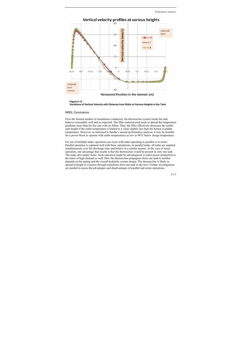
7/15/2019 Solar Storage 1019581



5-17

Figure 5-13Variations of Vertical Velocity with Distance from Walls at Various Heights in the Tank

NREL Conclusions

Over the limited number of simulations conducted, the thermocline system inside the tank behaves reasonably well and as expected. The filler material used tends to spread the temperaturegradients more than for the case with no fillers. Thus, the filler effectively decreases the usabletank height if the outlet temperature is limited to a value slightly less than the hottest availabletemperature. However, as indicated in Sandia’s annual performance analysis, it may be feasiblefor a power block to operate with outlet temperatures as low as 90°C below design temperature.

For use of multiple tanks, operation can occur with tanks operating in parallel or in series.

Parallel operation is captured well with these simulations. In parallel tanks, all tanks are emptied simultaneously over the discharge time and behave in a similar manner. In the case of seriesoperation, one advantage that results is that the thermocline would be present in only one tank.The tanks also empty faster. Such operation might be advantageous to tailor power production tothe times of high demand as well. How the thermocline propagates from one tank to another depends on the piping and the overall hydraulic system design. The thermocline is likely tospread in height as it passes through transitions from one tank to the next. Further investigationsare needed to assess the advantages and disadvantages of parallel and series operations.

7/15/2019 Solar Storage 1019581



5-18

The NREL results are limited in scope to a single tank undergoing the first cycle of dischargeover a period of 6 hours. The results show that the tank outlet temperature can begin to show adecline as early as 1.5 hours before the expected time of 6 hours (without diffusion at thethermocline interface). The presence of fillers promotes the diffusion and spread of thethermocline farther than for the case without fillers, reducing the effective thermal storage

capacity of the tank. The filler may reduce the quantity of salt needed, but may also increasethe cost of the tank.

Depending on how the plant is operated, the hot fluid may remain stagnant in the TES systemover many hours before being discharged. In such cases, the thermocline can be expected toincrease in width in proportion to the square root of the elapsed time. Longer discharge timeswill also increase the spread of the thermocline. Many cycles of charge/discharge would have to be simulated to arrive at the effective long-term behavior of the tank and its effective capacity.

Purdue Analysis

As a follow-on to the analysis performed by NREL, Purdue University performed additionalanalysis using computational fluid dynamics (CFD) to investigate the performance of thedischarge flow as well as the susceptibility to natural convection during dwell conditionsand over multiple cycles.

Tank Discharge Performance

For Purdue’s analysis of the thermocline tank discharge, the Case 5 design from Black &Veatch’s analysis was rendered and meshed with GAMBIT (Figure 5-14) and exported to theFLUENT CFD solver. To manage computational requirements, an axisymmetric boundary

condition was assumed along the tank centerline, which is a valid assumption as the transportequations contain no circumferential dependence. For the discharge half-cycle, a uniformvelocity inflow was assumed at the tank bottom. Inside the filler bed, flow momentum wascomputed according to Darcy’s Law with the Brinkman-Forchheimer extension. To track thethermal response of both the fluid and solid, co-located temperature storage was enacted throughout the domain mesh.

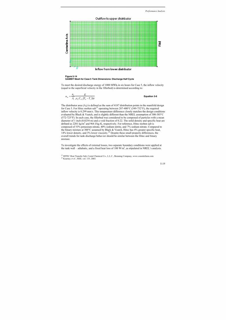
7/15/2019 Solar Storage 1019581



5-19

Figure 5-14GAMBIT Mesh for Case 5 Tank Dimensions: Discharge Half Cycle

To meet the desired discharge energy of 1000 MWht in six hours for Case 5, the inflow velocity(equal to the superficial velocity in the fillerbed) is determined according to:

( ) t T T C

E

A

Au

chPct

d

in Δ−=

1,1 ρ Equation 5-6

The distributor area (Ad ) is defined as the sum of 4187 distribution points in the manifold designfor Case 5. For Hitec molten salt

25operating between 287-400°C (549-752°F), the required

inflow velocity is 0.299 mm/s. This temperature difference closely matches the design conditionsevaluated by Black & Veatch, and is slightly different than the NREL assumption of 300-385°C(572-725°F). In each case, the fillerbed was considered to be composed of particles with a meandiameter of 1 inch (0.0254 m) and a void fraction of 0.22. The solid density and specific heat aredefined as 2201 kg/m3

and 964 J/kg-K, respectively. For reference, Hitec molten salt iscomposed of 53% potassium nitrate, 40% sodium nitrite, and 7% sodium nitrate. Compared tothe binary mixture at 300°C assumed by Black & Veatch, Hitec has 4% greater specific heat,14% lower density, and 3% lower viscosity.26 Despite these small property differences, the

overall trends for tank discharge behavior should be similar between the Hitec and binarymixture.

To investigate the effects of external losses, two separate boundary conditions were applied atthe tank wall – adiabatic, and a fixed heat loss of 100 W/m2, as stipulated in NREL’s analysis.

25 HITEC Heat Transfer Salt, Costal Chemical Co., L.L.C., Brenntag Company, www.coastalchem.com26 Kearney et al., JSSE, vol. 135, 2003.

7/15/2019 Solar Storage 1019581



5-20

Prior to discharge, the tank domain is initialized to 400°C (752°F). Cold fluid enters thelower boundary at the defined inflow velocity to simulate the discharge process. To track the progression of the heat exchange zone through the filler bed, the fluid temperature profiles atthe wall were plotted in Figure 5-15 for both wall boundary conditions considered. To improveunderstanding of the temperature loss, the axial centerline temperature profiles were also plotted

for the non-adiabatic case Figure 5-15(b). Also provided in Figure 5-16 is a contour plot of thefluid temperature at the end of the discharge half cycle for the 100 W/m2

wall condition.

As expected, the adiabatic tank maintained a fluid outflow at 400°C throughout the dischargehalf cycle. In contrast, the tank with a 100 W/m2 heat loss at the wall experienced sometemperature decay in both the hot and cold regions outside of the heat exchange zone. It should be noted, however, that this decay only exists very close to the tank wall. Beyond a distance of two feet from the wall, the fillerbed behaves similar to the adiabatic condition. Also, the decay islimited to a few degrees of temperature drop within the six-hour discharge period. As theminimum required fluid temperature for steam generation was defined as 364°C (687°F) in theDesign Requirements Table (see Appendix A), the non-adiabatic tank appears viable for the

desired operation.

7/15/2019 Solar Storage 1019581



5-21

(a) Adiabatic

(b) 100 W/m2 Heat Loss

Figure 5-15Fluid Temperature Profiles During a Discharge Half-Cycle for (a) an Adiabatic WallBoundary, and (b) a Heat Loss Boundary Condition.

7/15/2019 Solar Storage 1019581



5-22

Figure 5-16Fluid Temperature Distribution after Six Hours of Discharge for 100 W/m

2Heat Loss at the

Tank Wall

Some simplifying assumptions, such as the inclusion of monodisperse solid and uniform packing structure, were employed in the modeling results above. In addition, the discharge process has thus far incorporated the presence of the tank wall as two different boundaryconditions (adiabatic and fixed heat flux) along the fillerbed exterior. In reality, this surfacewould be coupled to the tank wall behavior, which is itself driven by external convection to the

surroundings. In the following discussion, more realistic tank operation is simulated by relaxingthese assumptions.

The preferred composition of a thermocline fillerbed is a mixture of rock and sand-scalequartzite, which improves the overall packing structure as well as the thermal exchange behavior at the solid interface. However, the use of sand creates potential for distributor clogging or entrainment during periods of tank operation (charge and discharge processes). These unwanted phenomena are avoided through the inclusion of rock stratification within the fillerbed. Near the two distributor manifolds on either end, the fillerbed is composed only of the rock-scalequartzite. Sandwiched between these two thin layers is the mixture of rock and sand. With thismodified structure, the rock layers isolate the sand and minimize contact with the distributor

manifolds.

To enforce this stratified structure within the CFD simulation, the tank domain is modified toinclude three different porous media regions for the rock and mixture, respectively, with distinct properties in each region. Given the dimensions for the Case 5 tank (152 ft diameter, 40 ftheight), the pure rock zones are defined at the lower and upper three feet of fillerbed while themixture is defined at the remaining interior. The equivalent diameters of the rock and sand are

7/15/2019 Solar Storage 1019581



5-23

defined as 1.905 cm and 0.2 cm, with a 2:1 ratio of rock to sand in the mixture region27. A Sauter mean diameter of 0.5 cm is calculated for the mixture to serve as an equivalent diameter for theregion. The void fractions of the rock and mixture regions are assumed to be 0.4 and 0.22,respectively.

With known geometry and void fraction, the permeability of both regions is determined as

28

:

( )3

32

1175 d

d K

−=

ε Equation 5-7

Due to its larger particle size and void fraction, the permeability of the rock is greater by a factor of 147.5, a two orders of magnitude difference. The increased permeability of the rock layer generates the potential for natural convection currents to develop along the tank wall due tolosses to the surroundings. These currents disrupt flow uniformity as well as the thermoclineregion itself by developing radial temperature gradients. To inhibit this behavior, the lower- permeability mixture region is extended along the wall surface to provide a buffer from the

rock layers. These extensions encompass a two-foot radial distance along the entire tank wall(Figure 5-17).

Figure 5-17CFD Domain for Simulation of Thermocline Tank Operation

27 Pacheco, J.E., Showalter, S.K., Kolb, W.J., 2002. Thermocline thermal storage system for parabolic trough plants.J. Sol. Energy Eng. 124, 153-159.28 Beckermann, C., and Viskanta, R., 1988, “Natural convection solid/liquid phase change in porous media,” Int. J.Heat Mass Transfer, 31, pp. 35–46.

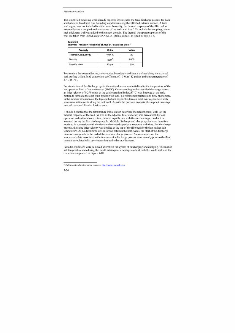
7/15/2019 Solar Storage 1019581



5-24

The simplified modeling work already reported investigated the tank discharge process for bothadiabatic and fixed heat flux boundary conditions along the fillerbed exterior surface. A tank wall region was not included in either case. In reality, the thermal response of the fillerbed toexternal losses is coupled to the response of the tank wall itself. To include this coupling, a twoinch thick tank wall was added to the model domain. The thermal transport properties of this

wall are taken from known data for AISI 347 stainless steel, as listed in Table 5-6.

Table 5-6Thermal Transport Properties of AISI 347 Stainless Steel

29

Property Units Value

Thermal Conductivity W/m-K 20

Density kg/m3 8000

Specific Heat J/kg-K 500

To simulate the external losses, a convection boundary condition is defined along the externaltank surface with a fixed convection coefficient of 10 W/m2

-K and an ambient temperature of 27°C (81°F).

For simulation of the discharge cycle, the entire domain was initialized to the temperature of thehot operation limit of the molten salt (400°C). Corresponding to the specified discharge power,an inlet velocity of 0.299 mm/s at the cold operation limit (287°C) was imposed at the tank bottom to simulate the cold fluid entering the tank. To resolve temperature and flow phenomenain the mixture extensions at the top and bottom edges, the domain mesh was regenerated withsuccessive refinements along the tank wall. As with the previous analysis, the implicit time step

interval remained fixed at 1.44 seconds.

It should be noted that the temperature initialization described included the tank wall. As thethermal response of the wall (as well as the adjacent filler material) was driven both by tank operation and external convection, thermal equilibrium with the surroundings could not beassumed during the first discharge cycle. Multiple discharge and charge cycles were thereforemodeled in succession until the domain developed a periodic response with time. For the charge process, the same inlet velocity was applied at the top of the fillerbed for the hot molten salttemperature. As no dwell time was enforced between the half cycles, the start of the discharge process corresponds to the end of the previous charge process. As a consequence, thetemperature data associated with time zero of a discharge process were actually prior to the flow

reversal associated with cycle transition in the thermocline tank.

Periodic conditions were achieved after three full cycles of discharging and charging. The moltensalt temperature data during the fourth subsequent discharge cycle at both the inside wall and thecenterline are plotted in Figure 5-18.

29 Online materials information resource, http://www.matweb.com

7/15/2019 Solar Storage 1019581



5-25

Figure 5-18Molten Salt Temperature Profiles during the Discharge Process

Results are shown for four different times during the discharge cycle (zero, two, four, and six

hours). Due to the large diameter of the thermocline tank, the influence of the externalconvection losses does not span the entire domain. Thus the centerline profiles remained withinthe hot and cold operation limits of the molten salt, as was the case with the previous adiabaticmodel. Due to the periodic nature of the charge-discharge cycles, it can be seen that the bottomof the fillerbed remained below the hot temperature limit at time zero of the discharge process.

Unlike the behavior along the centerline, the convection losses lead to significant cooling of themolten salt near the tank wall. As seen in Figure 5-18 above, the overall trend still shows anincreasing temperature with height from 150 to 350°C (302 to 662°F), consistent with theimposed temperature gradient across the fillerbed throughout the six-hour discharge. Apart fromthis trend, some spatial oscillations were present along the wall at the tank bottom. The negative

temperature gradient present at zero height (at the left end of the x-axis) is attributed to thecooling of the tank wall below the cold operation fluid temperature. Thus the entering cold fluid was warmer than the adjacent wall and led to additional cooling with height. The zero-time profile does not show such a negative temperature gradient, as it precedes flow reversal for discharge. The negative gradient is only seen at the later times.

7/15/2019 Solar Storage 1019581



5-26

The temperature fluctuation in space at the lower heights is attributed to flow disruptions in thesand-rock mixture extensions along the wall. While these were included with the intention of diminishing natural convection currents, the extensions also created vertical interfaces betweenthe rock and mixture layers. Due to the large disparity in permeability between the rock and mixture (two orders of magnitude as previously reported), the fluid prefers to travel through the

more conductive rock layer. At the vertical intersection of the different media, radial velocitiesdeveloped to allow transport of the fluid from the mixture region to the rock layer. As a result,a swirl flow developed on the rock side of the intersection while fluid flow in the mixture-extension region decayed to stagnant conditions. The temperature and velocity field in thelower mixture-extension region after six hours of discharge are provided in Figure 5-19.

Figure 5-19Temperature and Velocity Vectors along the Tank Wall in the Lower Mixture-ExtensionRegion

These radial velocities generate large vortices as well as flow stagnation within the lower extension. This stagnant region prevents heating of the fluid by advective transport; this region

thus experiences further cooling due to external wall heat loss. It is noted that the vortices exhibitturbulent characteristics and may not have been fully resolved despite the localized meshrefinement. As the fluid velocity and temperature are coupled, this may also lead to somediscrepancies in the temperature results; however, the effects of this very limited and smallregion are expected to be negligible, and the mesh size was chosen to limit computation time.

To illustrate the influence of the external losses and mixture and rock layers on the tank operation, the discharge temperature and axial velocity profiles along the top of the fillerbed

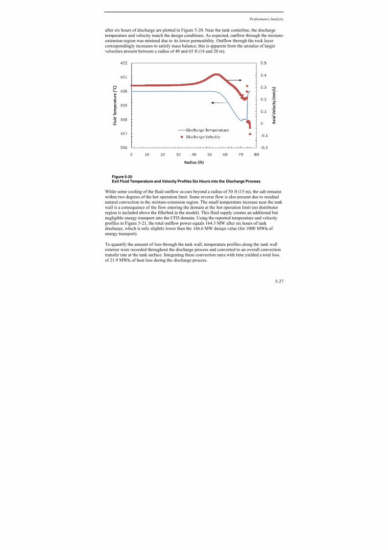
7/15/2019 Solar Storage 1019581



5-27

after six hours of discharge are plotted in Figure 5-20. Near the tank centerline, the dischargetemperature and velocity match the design conditions. As expected, outflow through the mixture-extension region was minimal due to its lower permeability. Outflow through the rock layer correspondingly increases to satisfy mass balance; this is apparent from the annulus of larger velocities present between a radius of 40 and 65 ft (14 and 20 m).

Figure 5-20Exit Fluid Temperature and Velocity Profiles Six Hours into the Discharge Process

While some cooling of the fluid outflow occurs beyond a radius of 50 ft (15 m), the salt remainswithin two degrees of the hot operation limit. Some reverse flow is also present due to residualnatural convection in the mixture-extension region. The small temperature increase near the tank wall is a consequence of the flow entering the domain at the hot operation limit (no distributor region is included above the fillerbed in the model). This fluid supply creates an additional butnegligible energy transport into the CFD domain. Using the reported temperature and velocity profiles in Figure 5-21, the total outflow power equals 164.3 MW after six hours of tank discharge, which is only slightly lower than the 166.6 MW design value (for 1000 MWht of

energy transport).

To quantify the amount of loss through the tank wall, temperature profiles along the tank wallexterior were recorded throughout the discharge process and converted to an overall convectiontransfer rate at the tank surface. Integrating these convection rates with time yielded a total lossof 21.9 MWht of heat loss during the discharge process.

7/15/2019 Solar Storage 1019581



5-28

Tank Behavior during Dwell Conditions

To simulate the thermal performance of the molten salt thermocline tank during dwell conditions between cycles, a constant heat flux of 100 W/m

2was applied at the tank wall to simulate

external losses. Near the wall, the molten salt is cooled, which generates a density gradient.

Buoyancy forces cause the denser fluid to flow down the wall and natural convection currentsdevelop in the tank. To accurately model the thermal performance of the thermocline tank withthis loss, the existing mesh was significantly refined at the tank wall to capture the velocity profiles associated with natural convection. The control volumes in this region were discretized to a length of 1.5 inches along the wall. Grid-independence was verified by using controlvolumes that are half this size (0.75 inch). A time step of 5 seconds was used for the duration of the dwell time.

To better approximate the no-flow conditions associated with the stagnant tank, the bottom of thefillerbed domain was changed to a wall boundary condition to prevent fluid from leaving thedomain. Moreover, due to the density change of the molten salt with temperature, the bulk

volume of the molten salt in the tank decreased with dwell time. In an actual thermocline tank,this reduction would generate some void space as the fluid level would drop to a lower tank height. To maintain continuity in the CFD model, the upper boundary condition is rendered permeable for additional molten salt to enter the domain and make up for the lost volumeassociated with the thermal contraction. While continuity is ensured in this manner, this permeability distorts the energy balance of the stagnant tank as the molten salt enters at the hottemperature and thus transports some additional energy into the domain. However, this artificialenergy transfer is approximately two orders of magnitude less than the fixed heat loss throughthe tank wall, and may be readily neglected.

A total dwell time of eight hours was simulated. The thermal response at the wall is shown in

Figure 5-21 at three different heights in the tank of 0, 20, and 40 feet (the bottom, middle, and top of the tank, respectively).

7/15/2019 Solar Storage 1019581



5-29

Figure 5-21Wall Temperature of the Thermocline Tank as a Function of Dwell Time

As seen in the plot, the top of the tank appears largely insensitive to the external tank losses. Itshould be remembered that the top of the tank was replenished with hot molten salt to make upfor the density change of the cooled fluid and may have distorted the local temperature values to

some extent. At the midpoint of the tank height, the wall temperature shows an initial decrease but decays to a constant temperature of approximately 395°C (743°F) after 3.5 hours of dwelltime. This temperature response can be attributed to the development of the natural convectionvelocity profile along the wall (shown in Figure 5-22). As the molten salt velocity along the walldevelops with time, the temperatures in the fully developed regions approach an approximatelysteady-state condition.

In contrast, the bottom of the tank continues to cool during the entire dwell time. Due to theimpermeable wall boundary condition stipulated for the bottom of the stagnant, the naturalconvection currents do not develop in this corner and the fluid remains relatively stagnant withtime. As such, this area of the tank is not replenished with warmer fluid from above and

continues to cool due to heat losses.

7/15/2019 Solar Storage 1019581



5-30

Figure 5-22Molten Salt Velocity Along the Tank Wall During the Initial Four Hours of Dwell Time

As with the tank discharge performance, further analysis was conducted by Purdue using morerealistic tank assumptions to further understand the dwell-time performance of the thermocline.Using the CFD model with rock stratification and heat losses at the tank wall, forced fluid flow

was stopped after a discharge half-cycle during periodic operation so that the tank thermalresponse during dwell conditions could be investigated. To prevent any outflow during this period, the bottom of the fillerbed was converted to a wall boundary condition. These conditionswere applied for four hours of dwell time. As with the discharge process, the total heat loss fromexternal convection was determined from the exterior temperature profiles and found to be 12.6MWht during the total period of the dwell time. The fluid temperature throughout the fillerbed atthis time is provided in Figure 5-23.

7/15/2019 Solar Storage 1019581



5-31

Figure 5-23Fluid Temperature Distribution after Four Hours of Dwell Conditions

The thermocline stratification is retained throughout most of the tank region with convectionlosses still being limited to the region very close to the tank wall. To resolve the externalconvection effects, the temperature response at five height locations along the interior wallsurface is plotted in Figure 5-24 against dwell time.

Figure 5-24Interior Wall Temperatures in the Thermocline Tank during the Dwell Time

7/15/2019 Solar Storage 1019581



5-32

The largest temperature change occurs at the bottom of the fillerbed during the first hour of dwellconditions. As mentioned in the discussion of the discharge cycle, the bottom of the fillerbed wasinfluenced by molten salt entering at a warmer temperature than the adjacent wall. As this inflowwas not present during the dwell state, the local fillerbed could no longer support a greater temperature than the surroundings which led to the cooling shown in the figure. After this initial

effect, the bottom (as well as the other wall locations) maintained a minimal temperaturedecrease with time.

Discussion and Comparison of NREL and Purdue Thermal Performance Results

Comparing the results from the models developed at Purdue University with the work performed by NREL, discrepancies are evident with respect to the overall performance predictions of thethermocline system. The reasons for the differences between the two sets of predictions are provided below, for both the discharge model and the natural convection analysis.

Discharge Cycle Model

In the NREL thermocline discharge model, the superficial velocity (the product of real fluid velocity and fillerbed void fraction) was constrained to a fluid flow residence time equal to thetank discharge time. For the specified liquid height and discharge time of 14 meters and 6 hours,respectively, the resultant superficial velocity was 0.648 mm/s. The real velocity was thenvaried according to the user-defined bed void fraction. In reality, the fluid flow does not have a“superficial” residence time in the tank. The residence time of the fluid is the ratio of the tank height to the real fluid velocity. The merit of superficial velocity in a porous medium is to correctfor the deviation in mass flow due to the presence of solids in the cross-sectional tank area. Thus by constraining the superficial velocity, the residence time of the fluid flow in the tank still

varied with the user-defined void fraction.

In the Purdue analysis, the fluid velocity was determined from the required discharge power and the diameter of the tank and not by constraining it to a residence time. As thermocline tanks aresized for a required storage energy and cycle time, the discharge power is subsequently equal tothe ratio of this energy to the cycle time. In addition, the power associated with the dischargeflow can also be related to the molten salt mass flow rate as:

( )chPT T C mP −= & Equation 5-8

For known material properties and tank area, this mass flow rate can be converted to a discharge

outflow velocity using:

UAmh ρ =& Equation 5-9

This would be the velocity at the outflow of the fillerbed, and therefore equal to the superficialvelocity of the molten salt inside the fillerbed. Using the model parameters listed by NREL for a50 ft diameter tank, the superficial velocity would be 0.387 mm/s to satisfy the outflow power associated with the tank energy and discharge cycle time. This result is entirely independent of

7/15/2019 Solar Storage 1019581



5-33

the tank height. Applying the artificial residence time constraint instead generated a superficialvelocity that is 67% greater than necessary for nominal tank operation. As a consequence, theoutflow supplied excess thermal power which drained the stored tank energy too quickly, asnoted by the sharp temperature decrease at 4.5 hours in Figure 5-10.

Dwell-Time Model

In both the NREL and Purdue models for a stagnant tank filled with hot molten salt, naturalconvection currents are generated by applying a constant heat flux of 100 W/m2 at the tank wallto simulate external losses to the surroundings. In the NREL simulation of the wall heat transfer,the left side of the domain has a fixed temperature imposed, which causes a big slope in theliquid temperature profiles which does not truly represent the real situation. Since the heattransfer in the fluid region is dominated by convection, it is not likely for the fluid to have asudden change in temperature in the regions far away from the wall.

Nomenclature

A AreaCP Specific heatd Filler diameter D Diameter E EnergyK Permeability p PressureQ Flow rateT Temperature

u Velocity

Greek

ε Void fractionλ Friction factor μ Viscosity

ρ Density

Subscript

l fluid c Cold

d Distributor h Hotm Meant Tank

7/15/2019 Solar Storage 1019581


7/15/2019 Solar Storage 1019581


6-1

6 CONCLUSIONS

Thermal energy storage holds the promise of providing an efficient and cost-effective way totransform solar thermal energy from a variable resource into a firm, more dispatchable source of electricity. Studies have shown that a thermal energy storage system improves the performanceof a solar thermal plant by smoothing power production and/or allowing it to continue during brief periods of lost solar resource, such as intermittent cloud cover, or into the evening hourswhen the solar resource is no longer available. Used in this way, thermal storage can increasethe utilization of the power block and the annual capacity factor of a CSP facility, decrease thelevelized cost of electricity produced by the plant, and facilitate the incorporation of solar

thermal power plants into the utility grid.

This study showed the potential of thermocline storage systems to significantly reduce the costof TES. The potential cost advantage for the thermocline is the use of a single tank instead of two tanks and a much lower volume of solar salt. For a 1000 MWht system, this means a tank volume of 20,600 m3 instead of two 16,300 m3 tanks, and a salt volume of roughly 5,000 m3 instead of about 18,000 m

3for the two tanks. These systems require relatively simple designs,

involving chemically inert media that remain in a single phase throughout the storage chargingand discharging process. The direct central receiver thermocline systems appear to be thelowest cost option on an absolute basis. The study confirmed the feasibility of achieving total(direct & indirect) capital costs below $35/kWht and $70/kWht for direct and indirect systems,respectively, compared to $50/kWht and $90/kWht for the equivalent two-tank cases. For the500-1500 MWht size range the indirect parabolic trough thermocline systems have the greatestcost benefit on a percentage basis compared to two-tank; the 1500 MWht indirect trough case hasa 37% cost reduction compared to 20% for the direct central receiver. For the larger tank sizes,3000-3500 MWht the direct systems show greater benefit than the indirect systems, a 33% vs.23% advantage over the equivalent two-tank designs for the 3500 MWht cases. For all systems500 MWht and larger, the cost benefit was 20% or more compared to the corresponding two-tank designs. In the future a direct storage system for parabolic trough also should be considered tofurther reduce cost and efficiency losses. Developing cost effective trough storage is a significantR&D challenge that will likely require development of a new lower cost HTF.

On the spectrum of commercial maturity, the two-tank indirect molten salt system represents

the current state-of-the-art for thermal energy storage, with two projects recently completed and several more scheduled to begin construction. Two-tank direct systems are close behind, both for central receiver CSP plants and parabolic trough plants if molten salt proves viable in a parabolictrough collector field. The logical next step for the thermocline system is a pilot plant or a smallcommercial unit that can validate the operation of the storage system outside of the laboratory.Given the expanding number of CSP plant deployments, there is ample room for further development in the field of thermal energy storage. In addition to further testing and validationin the field, standardized design and modeling procedures would be a valuable addition to TES

7/15/2019 Solar Storage 1019581


Conclusions

6-2

system design to improve the design process and speed up production and deployment of thermalenergy storage systems. The development of the thermocline TES would benefit greatly fromimproved modeling and tank design techniques, which would offer a more complete picture of design and performance. Testing and operation of a larger scale pilot thermocline will alsodemonstrate the capabilities of the system.

Next Steps

Two potential courses of action are under consideration for further development of thethermocline technology under EPRI’s Generation Technology Industry Demonstration Program.

• The first is a front-end engineering design of a thermocline storage system to reduce thespread in the budget estimation and develop a complete design for the first commercial-scaledemonstration plant. This follow-on study would include the following:

– Detailed design of storage tank shell, reinforcements, internal structures, distributorssystems, civil foundations, etc.

– Detailed process diagrams and P&IDs – Main equipment specifications for salt pumps, heat exchangers, and auxiliary equipment

– Interconnection with the solar plant

– Operating modes and transient analysis

– Project schedule

• In the second approach EPRI would develop a small capacity pilot project that could resolveoutstanding R&D questions. This project would likely be done in collaboration with thenational laboratories and would include testing and modeling activities. The equipment could potentially be sited at the Solar Technology Acceleration Center (SolarTAC) in Colorado, atSandia in Albuquerque, or at a thermal plant (solar or fossil). Sandia plans to study thermal

ratcheting in 2010. Detailed finite element analysis (FEA) models of various thermoclinetank geometries, such as vertical and sloped tank walls, will be analyzed with ANSYSsoftware. The temperature difference between the top and bottom of the tank will be varied from 100°C (today's trough) to 350°C (next-generation super-critical tower). Low-costmethods of eliminating the thermal ratcheting issue will be proposed, e.g., sloped walls,inserts, etc. If the analytical work indicates that ratcheting is a manageable issue, Sandia plans to build a lab-scale prototype to validate the FEA models of the most promisingsolution(s) in 2011. Further work is ongoing at NREL to develop a more universal fit for evaluation of thermocline-based thermal energy storage systems. NREL plans to develop aset of approximations for the thermocline tank behavior for a variety of tank and filler geometries, heat-transfer parameters, and operating conditions. The objectives of the pilot

project would include:

– Validate model performance across different operating strategies

– Determine potential impact, if any, due to thermal ratcheting

– Review performance of active components (pumps, valves, seals, etc.) operating inmolten salt environment

– Examine transients and fatigue effects on materials due to thermal cycling

7/15/2019 Solar Storage 1019581


A-1

A DESIGN REQUIREMENTS

Table A-1Design Requirements

ITEM REQUIREMENT

ApproachDesign single thermocline tank or multiplemodular thermocline tanks for each designcase as appropriate.

Storage Fluid Molten binary nitrate salts: 60%Na/40%K

Density at 300°C (572°F) 1830 kg/m3

Viscosity at 300°C (572°F) 3.26 cP

Heat Capacity at 300°C (572°F) 1,495 J/kg-K

Filler 75% of the volume filled with rocks and sand

Material Quartzite (SiO2) 1- 2" sphere equivalent

Rock density 165 lbm/ft3

HOT-Top of the tank 585°C (1085°F)Design Storage Temperatures (Direct)

COLD-Bottom of the tank 287°C (550°F)HOT-Top of the tank 400°C (752°F)

Design Storage Temperatures (Indirect)COLD-Bottom of the tank 287°C (550°F)

Working Capacity: Full Power TES Hours SIX (6) HOURS

Minimum Heel 0.9 m (3 feet)

Cover GasVented to atmosphere; NO

Xscrubbing system

for initial salt fill

Site Conditions (See Environmental ConditionsDocument below for additional details )

Seismic API 650 Zone 3

Wind 40.2 m/sec (90 mph)

Soil 480 kPa (10,000 psi) allowable bearing

Instrumentation Level, pressure and temperatures indication

7/15/2019 Solar Storage 1019581


Design Requirements

A-2

Table A-1Design Requirements (Continued)

ITEM REQUIREMENT

Tank Valving Vented to atmosphere

AuxiliariesDetermined that no active convection coolingis required

Tank warm-up/start-up system – hot air toheat tank internals, filler, etc.

Tank thermal insulation and supportingstructures as required

Earthen impoundment dikes to contain a saltspill of the complete content of the tank aboveground

Upper and lower manifolds and internalplumbing to minimize entrainment

Inlet/outlet ports design details (orientationand geometry including baffles)

Salt drain tank for gravity drain of auxiliarypiping and heat exchangers, if required

Auxiliary piping, hot/cold pumps and valves asrequired by system design.

Auxiliary salt melter

BOP-salt-to-steam heat exchanger (solar

steam generator); LMTD 7°C-salt side

System heat exchanger with solar field HTF-(thermal oil) for indirect TES system; LMTD7°C-salt side

Any other auxiliary system required for thestart-up/operation of the TES thermoclinesystem (e.g., salt maintenance system)

Design Life 30 years

Design Standards

Basic Design API 650

Seismic Design API 650 APP E

Foundations ACI 318

Piping B 31.1

High Temperature Allowable Stresses ASME Section VIII

7/15/2019 Solar Storage 1019581


Design Requirements

A-3


ITEM REQUIREMENT

TES Storage Tank Design Vertical, cylindrical with dome roof

Tank ullage space provided over the uppermanifold

Dome roofs self supporting

Tank height added as freeboard to allow forsalt sloshing during safe shutdownearthquake (SSE)

Tank bottom design developed by B&V tominimize thermal stresses (e.g., sloped-wallconical bottom concept) and cost

Tank Height/Diameter Optimized for capacity vs. cost

Taller thermocline tanks with smallerdiameters are favored over shorter tanks withlarger diameters. Soil bearing capacity limitstank height.

Piping/Valves/Instrumentation Heat Tracing

All TES salt piping, valves, instrumentation tobe heat traced to prevent salt freeze-up duringoperation and allow pre-heating during start-up.

Expansion Joints Expansion joints included, if required

Solar Steam Generator Subsystem Only the molten salt side

Steam Generator Configuration Forced recirculation

Heat Exchanger Welded plate and frame

Thermal Rating (MWt) 16.7 to 583.3 MWt

LMTD 5°C

Materials

Tanks operating up to 425°C (800°F) Carbon steel SA-285C

Tanks operating above 425°C up to 560°C (1040°F) Stainless steel SA-240-347

Side Wall Thermal Insulation Mineral wool

Base InsulationCombination of foam glass and insulating firebrick

Salt Cold Piping ASTM A 106 Grade B seamless carbon steel

Salt Hot Piping ASTM A312, TP 304 seamless stainless steel

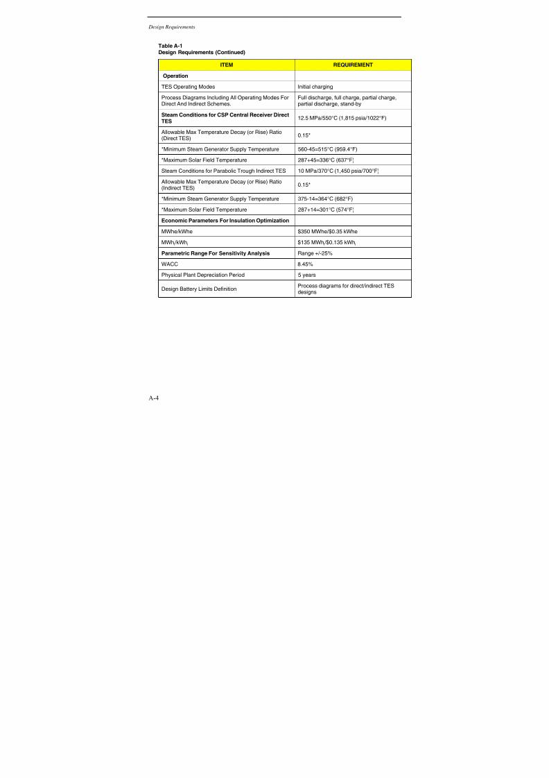
7/15/2019 Solar Storage 1019581


Design Requirements

A-4


ITEM REQUIREMENT

Operation

TES Operating Modes Initial charging

Process Diagrams Including All Operating Modes ForDirect And Indirect Schemes.

Full discharge, full charge, partial charge,partial discharge, stand-by

Steam Conditions for CSP Central Receiver DirectTES

12.5 MPa/550°C (1,815 psia/1022°F)

Allowable Max Temperature Decay (or Rise) Ratio(Direct TES)

0.15*

*Minimum Steam Generator Supply Temperature 560-45=515°C (959.4°F)

*Maximum Solar Field Temperature 287+45=336°C (637°F)

Steam Conditions for Parabolic Trough Indirect TES 10 MPa/370°C (1,450 psia/700°F)

Allowable Max Temperature Decay (or Rise) Ratio(Indirect TES)

0.15*

*Minimum Steam Generator Supply Temperature 375-14=364°C (682°F)

*Maximum Solar Field Temperature 287+14=301°C (574°F)

Economic Parameters For Insulation Optimization

MWhe/kWhe $350 MWhe/$0.35 kWhe

MWht /kWht $135 MWht /$0.135 kWht

Parametric Range For Sensitivity Analysis Range +/-25%

WACC 8.45%

Physical Plant Depreciation Period 5 years

Design Battery Limits DefinitionProcess diagrams for direct/indirect TESdesigns

7/15/2019 Solar Storage 1019581


Design Requirements

A-5

7/15/2019 Solar Storage 1019581


Design Requirements

A-6

7/15/2019 Solar Storage 1019581


Design Requirements

A-7

7/15/2019 Solar Storage 1019581


Design Requirements

A-8

7/15/2019 Solar Storage 1019581


Design Requirements

A-9

7/15/2019 Solar Storage 1019581


Design Requirements

A-10

7/15/2019 Solar Storage 1019581


B-1

B THERMOCLINE PROCESS FLOW DIAGRAMS

7/15/2019 Solar Storage 1019581


Thermocline Process Flow Diagrams

B-2

Figure B-1Indirect Thermocline Process Flow Diagram

7/15/2019 Solar Storage 1019581


T

Figure B-2Direct Thermocline Process Flow Diagram

7/15/2019 Solar Storage 1019581


7/15/2019 Solar Storage 1019581


C-1

C HEAT AND MATERIAL BALANCE

Figure C-1Heat and Material Balance Spreadsheet, Page 1

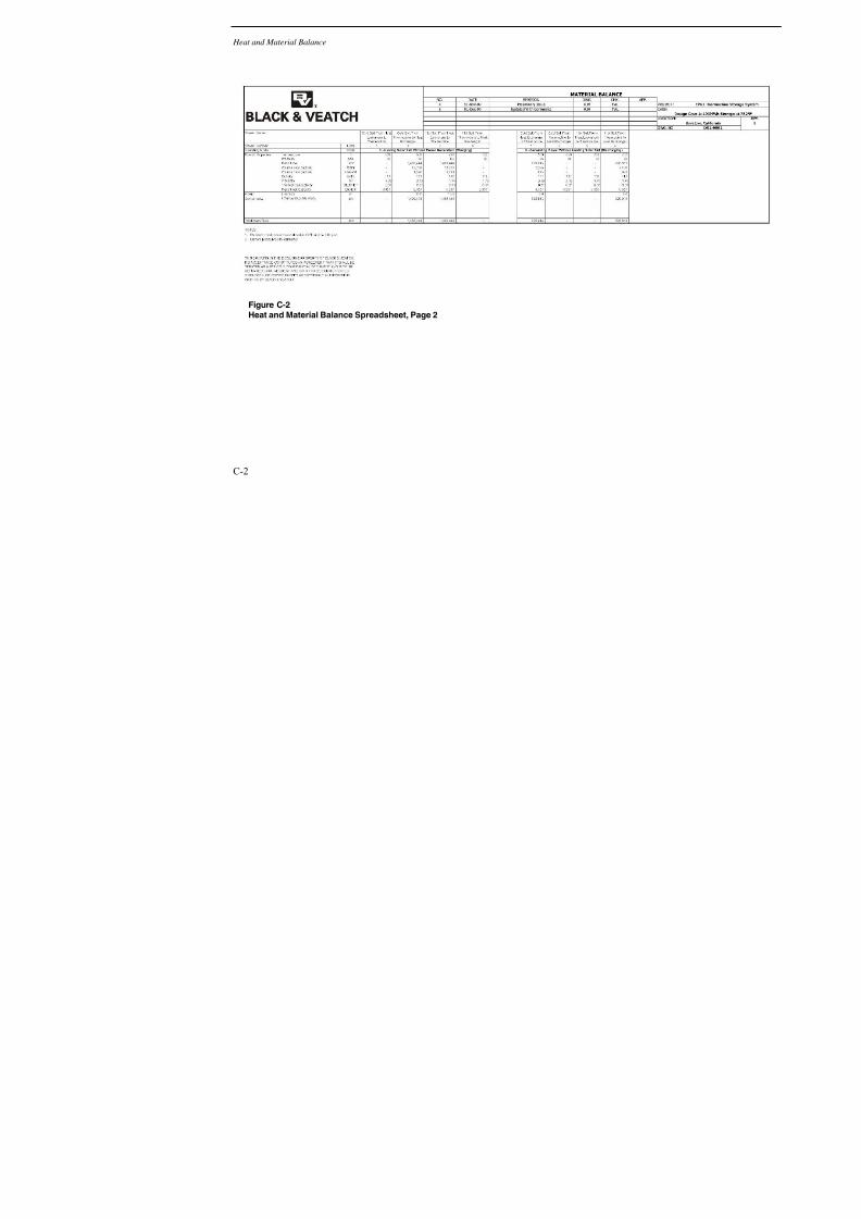
7/15/2019 Solar Storage 1019581



C-2


7/15/2019 Solar Storage 1019581



7/15/2019 Solar Storage 1019581



C-4


7/15/2019 Solar Storage 1019581



7/15/2019 Solar Storage 1019581



C-6


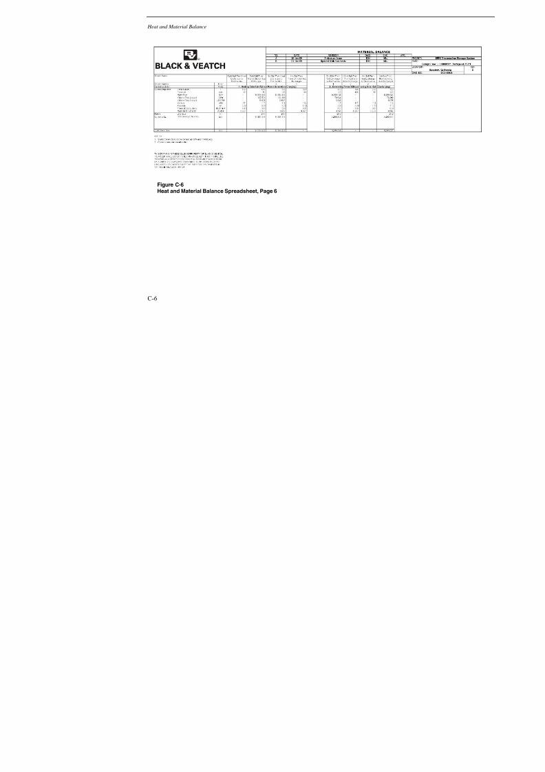
7/15/2019 Solar Storage 1019581



7/15/2019 Solar Storage 1019581



C-8


7/15/2019 Solar Storage 1019581



7/15/2019 Solar Storage 1019581


D-1

D MAXIMUM TANK HEIGHT CALCULATIONS

This analysis is a reference to a civil engineering study prepared by B&V. The goal of thisanalysis was to determine the maximum feasible height of a thermocline tank.

In designing a thermocline system, it is desirable to maximize the height of the storage tank.Increasing the height of the tank improves the efficiency such that the volume of the tank can bereduced. The smaller tank volume means that less salt is required to store a given amount of energy, which reduces the overall cost of the project. The goal of this study is to determine themaximum feasible tank height for this project.

The main consideration in this study is the amount of pressure that the soil can support. Based onthe environmental conditions of Barstow California, it was found that a spread foundation cansupport approximately 10,000 lb/ft

2.

The bearing stress was calculated for tank diameters of 70, 75, 80, and 85 feet. The stress wascalculated for all heights between 8 and 40 feet tall. It should be noted that this is a liquid height,and this does not include any empty space at the top of the tank. This space does not contributesignificantly to the bearing pressure. The reference parameters for the calculations include:

• Dia (ft): The diameter of the thermocline tank, in feet

• Height (ft): The liquid height in the thermocline tank

• Area (ft2): The area of the tank foundation

• Weight (K): The total mass of the thermocline tank contents in Kips (1,000 lb increments)

• V (K): UBC 97 Limiting base sheer

• OTM (ft-K): Overturning moment

• P/A (K/ft2): The weight of the tank divided by the area

• S (ft3): Section modulus (inertia / distance to the edge of the tank)

• M/S (K/ft

2

): The overturning moment divided by the section modulus• Bearing (ksf): The estimated bearing pressure on the soil

• e/D < 0.123: The overturning moment divided by the weight of the structure * diameter

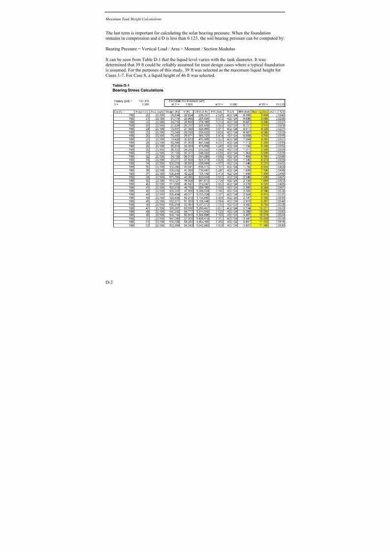
7/15/2019 Solar Storage 1019581


Maximum Tank Height Calculations

D-2

The last term is important for calculating the solar bearing pressure. When the foundationremains in compression and e/D is less than 0.123, the soil bearing pressure can be computed by:

Bearing Pressure = Vertical Load / Area + Moment / Section Modulus

It can be seen from Table D-1 that the liquid level varies with the tank diameter. It wasdetermined that 39 ft could be reliably assumed for most design cases where a typical foundationis assumed. For the purposes of this study, 39 ft was selected as the maximum liquid height for Cases 1-7. For Case 8, a liquid height of 46 ft was selected.

Table D-1Bearing Stress Calculations

7/15/2019 Solar Storage 1019581



D-3

Table D-1Bearing Stress Calculations (Continued)

7/15/2019 Solar Storage 1019581



D-4


7/15/2019 Solar Storage 1019581



D-5


7/15/2019 Solar Storage 1019581



D-6


7/15/2019 Solar Storage 1019581



D-7


7/15/2019 Solar Storage 1019581



D-8


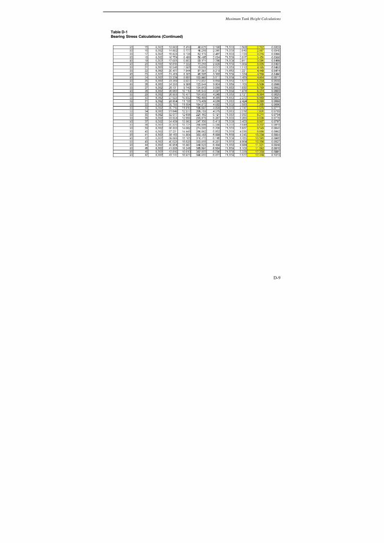
7/15/2019 Solar Storage 1019581



D-9


7/15/2019 Solar Storage 1019581



D-10


7/15/2019 Solar Storage 1019581



D-11


7/15/2019 Solar Storage 1019581


7/15/2019 Solar Storage 1019581


E-1

E STEEL SENSITIZATION

If stainless steel is heated above 500°C (932°F) there is a risk that chrome may react with carbonto form chrome carbides. These chrome carbides deplete the surrounding areas of chrome, whichdecreases the corrosion resistance of the steel. This phenomenon is called sensitization. Over time, this leads to preferential corrosion of the affected area, which can lead to cracking and possible failure of the steel.

This phenomenon was investigated in an article that was published in a Nippon Steel TechnicalReport in 2004.

30The most relevant piece of information provided in this article is a graph

indicating the temperatures and conditions at which sensitization occurs.

Figure E-1Steel Sensitization

The thermocline process operates at 560°C (1040 °F). At these conditions, Stainless Steel 347(SUS347HTB in Figure E-1) became sensitized after approximately 20 hours of exposure. For this reason, Black & Veatch selected Inconel 625 for the high temperature thermocline process.The addition of significant amounts of nickel, chrome, niobium, and titanium decrease thesensitization potential of the metal.

30 “Development of New Austenitic Stainless Steel Boiler Tube with High Strength at Elevated Temperatures and Intergranular Corrosion Resistance.” Nippon Steel Technical Report No 90,: July 2004.

7/15/2019 Solar Storage 1019581


7/15/2019 Solar Storage 1019581


F-1

F EQUIPMENT LIST

7/15/2019 Solar Storage 1019581


F-2

Table F-1Equipment List Summary

EPRI Thermocline Study BLACK & VEATCH

Barstow, California Equipment List Summary

Project Number 165470.0010

Design

Case

Working

Storage

(MWh) # Tanks

Tank ID

(ft)

Tank

Height

(ft)

Surge

Tank ID

(ft)

Surge Tank

Height (ft)

Hot Salt Flow

Rate (lb/hr)

Number of

Operating Hot

Pumps

Hot Pump

Motor Size

(hp)

Hot Pump

ΔP (psia)

Cold Salt Flow

Rate (lb/hr)

Number o

Operating C

Pumps

1 100 1 48 40 4.0 10.0 1,488,444 1 75 60 826,913

2 100 1 31 40 5.0 8.0 596,493 1 30 60 331,385

3 500 1 107 40 7.5 10.0 7,442,220 3 125 60 4,134,567

4 500 1 69 40 8.0 10.0 2,982,463 1 150 60 1,656,924

5 1000 1 152 40 11.0 10.0 14,884,441 5 150 60 8,269,134

6 1000 1 98 40 11.0 10.0 5,964,926 2 150 60 3,313,848

7 3000 2 160 50 20.0 16.0 44,653,323 13 200 60 24,807,402

8 3000 1 155 47 14.0 16.0 17,894,777 6 150 60 9,941,543

7/15/2019 Solar Storage 1019581


7/15/2019 Solar Storage 1019581


Equipment List

F-4

Table F-3Equipment List Summary – 100 MWh

tDirect Central Receiver


Barstow, California PRELIMINARY Equipment List

Project Nu mber 165470.0010 Design Case 2: 100MWh Storage at 1040°F

Size Electrical

Tag Service Qty Type Parameter 1 Parameter 2 MOC Oper. Conn.

(HP) (HP)

VESSELS & TANKS

V-101 Hot Molten Salt Surge Tank 1 Vertical Inconel 625

V-102 Cold Molten Salt Surge Tank 1 VerticalCarbonSteel

V-103 Thermocline Storage Tank 1 API-650 Inconel 625

V-104 Salt Melting Sump 1 VerticalCarbon

Steel

HEAT EXCHANGERS & FIRED EQUIPMENT

CarbonSteel

CarbonSteel

ROTATING EQUIPMENT

P-101 A/B Hot Molten Salt Pump 2Vertical

SubmergedBy vendor 30.0

P-102 A/B Cold Molten Salt Pump 2Vertical


P-103 Salt Charging Pump 1 VerticalSubmerged By vendor 7.5

B-101 Quartz Preheating Blower 1 RotaryCarbonSteel

125.0

Tank Packing and Process Chemicals

M-101 Quartzite Packing 1700 ton By vendor

M-102 Molten Salt 480 ton By vendor

Void Fraction:0.25

Density: 165 lb/ft3

60:40 wtNaNO3:KNO3

Standard Grade

TL-TL = 8' ID =5'

TL-TL = 8' ID =5'

TL-TL =40'

Gas FiredHeater

TL-TL = 6'

ID =31'

ID =6'

4.6 MMBtu/h

Duty

Electric

3.4 MMSCFD dp =10 inH2O

709 gpm dP =60 psi

637 gpm dP =260 psi

94 gpm dP =60 psi

F-101 Quartz Preheater 1

E-102 Salt Melting Heater 175 kW

Duty

7/15/2019 Solar Storage 1019581


7/15/2019 Solar Storage 1019581


Equipment List

F-6

Table F-5Equipment List Summary – 500 MWht Direct Central Receiver



Project Number 165470.0010 Design Case 4: 500MWh Sto rage at 1040°F

Size Electrical


(HP) (HP)

VESSELS & TANKS





Steel


CarbonSteel

CarbonSteel

ROTATING EQUIPMENT





P-103 Salt Charging Pump 1

Vertical

Submerged By vendor 25.0


550.0




Void Fraction:0.25

Density: 165 lb/ft3

60:40 wtNaNO3:KNO3

Standard Grade


3545 gpm dP =60 psi

3185 gpm dP =260 psi

472 gpm dP =60 psi

F-101 Quartz Preheater 115.6 MMBtu/h

DutyGas Fired

Heater

ID =69'

TL-TL = 8' ID =10'

TL-TL = 8' ID =10'

TL-TL =40'

TL-TL = 10' ID =10'

E-102 Salt Melting Heater 1 ElectricDuty

350 kW

7/15/2019 Solar Storage 1019581


7/15/2019 Solar Storage 1019581


Equipment List

F-8

Table F-7Equipment List Summary – 1000 MWh

tDirect Central Receiver



Project Number 165470.0010 Design Case 6: 1000MWh Storage at 1040°F

Size Electrical


(HP) (HP)

VESSELS & TANKS




V-104 Salt Melting Sump 1 VerticalCarbonSteel


CarbonSteel

CarbonSteel

ROTATING EQUIPMENT





P-103 Salt Charging Pump 1Vertical



1100.0




Void Fraction:0.25

Density: 165 lb/ft3

60:40 wtNaNO3:KNO3

Standard Grade

TL-TL = 8' ID =11'

TL-TL = 8' ID =11'

TL-TL =40'

Gas FiredHeater

TL-TL = 10'

ID =98'

ID =14'

31.3 MMBtu/h

Duty

Electric


3185 gpm dP =60 psi


944 gpm dP =60 psi

F-101 Quartz Preheater 1

E-102 Salt Melting Heater 1700 kW

Duty

7/15/2019 Solar Storage 1019581


7/15/2019 Solar Storage 1019581


Equipment List

F-10

Table F-9Equipment List Summary – 3000 MWht Direct Central Receiver


Barstow, California PRELIMINARY Equipment L ist

Project Number 165470.0010 Design Case 8: 3000MWh Storage at 1040°F

Size Electrical


(HP) (HP)

VESSELS & TANKS





Steel


CarbonSteel

CarbonSteel

ROTATING EQUIPMENT





P-103 Salt Charging Pump 1Vertical

Submerged By vendor 60.0


1700.0




Void Fraction:0.25

Density: 165 lb/ft3

60:40 wtNaNO3:KNO3

Standard Grade


3545 gpm dP =60 psi


1416 gpm dP =60 psi

F-101 Quartz Preheater 147.6 MMBtu/h

DutyGas Fired

Heater

ID =155'

TL-TL = 16' ID =11'

TL-TL = 16' ID =11'

TL-TL =47'

TL-TL = 10' ID =17'

E-102 Salt Melting Heater 1 ElectricDuty

1100 kW

7/15/2019 Solar Storage 1019581


G-1

G COMPLETE DESIGN ESTIMATE

The cost estimates indicate that the proposed thermocline thermal energy storage system has the potential to significantly reduce TES costs compared to a two-tank storage system. There is awide cost range that depends largely on the scale of the project and the operating temperature.The cost estimates developed in this study include both direct and indirect costs with acontingency of 15% and sales tax. They are presented in January 2010 dollars.

The results in Figure G-1 and Figure G-2 represent the total installed capital costs (direct and indirect) for the thermocline and two-tank systems, respectively, including 15% contingency and

sales tax. Table G-1, and Table G-2 show the detailed breakdown of these costs. Values for thesystems not included in the tables were calculated through linear interpolation or linear extrapolation.

Estimates provided in Table G-1 and Table G-2 have an uncertainty of approximately +40%/-20% in accordance with AACE Class 4 estimate. The uncertainty with these estimates can bereduced with additional design or demonstration of the concepts identified in this report. Detailed modeling, design or demonstration of the following items will likely be necessary to confirm theconceptual designs presented here:

• Dynamic modeling of thermocline

• Thermal ratcheting

• Tank materials

• Distributor design

• Other tank internals, including structural supports

7/15/2019 Solar Storage 1019581


Complete Design Estimate

G-2

$24,613,000

$104,553,000

$215,425,

$84,219,000

$53,146,000$66,000,000

$45,955,000

$30,503,000$13,184,000

$-

$50,000,000

$100,000,000

$150,000,000

$200,000,000

$250,000,000

$300,000,000


T o t a l C a p i t a l C

o s t

Indirect Trough Thermocline

Direct Central Receiver Thermocline

100 MWh t 500 MWh t 1500 MWh t 3000 1000 MWh t

Figure G-1Total Capital Cost (Direct & Indirect) for Thermocline Design Cases

7/15/2019 Solar Storage 1019581


$166,500,000

$284,45

$27,532,000

$71,348,000

$115,525,000

$18,059,000

$38,783,000$57,139,000

$82,500,000

$-

$50,000,000

$100,000,000

$150,000,000

$200,000,000

$250,000,000

$300,000,000

$350,000,000


T o t a l C a p i t a l

C o s t

Indirect Trough Two-Tank

Direct Central Receiver Two-Tank

100 MWht 500 MWht 1500 MWh t 30001000 MWh t

Figure G-2Total Capital Cost (Direct & Indirect) for Two-Tank Design Cases

7/15/2019 Solar Storage 1019581


7/15/2019 Solar Storage 1019581


Table G-1Capital Costs for Thermocline Tank Designs (continued)

ThermoclineDesign Estimate

Design Case100 MWht Indirect

Trough100 MWht DirectCentral Receiver

500 MWht IndirectTrough

500 MWht DirectCentral Receiver

1000 MWht Indirect Trough

1000 MWht DCentral Rece

Indirect

Contingency (15%on Direct) $2,580,000 $1,259,000 $5,858,000 $3,166,000 $9,359,000 $4,790,00

Sales Tax (8.75%on material) $1,100,000 $944,000 $1,660,000 $1,990,000 $2,860,000 $3,580,00

Engineering - (3%of direct) $516,000 $252,000 $1,172,000 $633,000 $1,872,000 $958,000

ConstructionIndirects IncludingScaffolding) $1,720,000 $839,000 $3,905,000 $2,110,000 $6,239,000 $3,195,00

ConstructionManagement $1,500,000 $1,500,000 $1,500,000 $1,500,000 $1,500,000 $1,500,00

Indirect Subtotal $7,416,000 $4,794,000 $14,095,000 $9,399,000 $21,830,000 $14,023,00

Total $24,613,000 $13,184,000 $53,146,000 $30,503,000 $84,219,000 $45,955,00

Capital InvestmentPer MWProduction $1,476,780 $791,040 $637,752 $366,036 $505,314 $275,730

Capital InvestmentPer kWh

tStorage $246 $132 $106 $61 $84 $46

7/15/2019 Solar Storage 1019581


7/15/2019 Solar Storage 1019581


Table G-2Capital Costs for Two-Tank Designs (Continued)

Design Case100 MWht

Indirect Trough

100 MWht Direct Central

Receiver500 MWht

Indirect Trough


Receiver1000 MWht

Indirect Trough


Receiver3

Ind

Construction Indirects(Including Scaffolding) $2,450,000 $3,870,000 $6,120,000 $6,400,000 $5,130,000 $3,950,000 $

ConstructionManagement $1,500,000 $1,500,000 $1,500,000 $1,500,000 $1,500,000 $1,500,000 $

Indirect Subtotal $9,795,000 $8,775,000 $20,350,000 $15,100,000 $28,230,000 $18,000,000 $

Total $27,532,000 $18,059,000 $71,348,000 $38,783,000 $115,525,000 $57,139,000 $2

Capital Investment PerMW Production $1,651,920 $1,083,540 $856,176 $465,396 $693,150 $342,834

Capital Investment PerkWh

tStorage $275 $181 $143 $78 $116 $57

7/15/2019 Solar Storage 1019581



G-8

Table G-3 provides a summary of the total installed capital costs on a per-kilowatt-hour-thermal basis.

Table G-3Molten Salt Thermocline Storage Capital Costs

Storage Capacity(MWh

t)


ThermoclineCost ($)

Cost Per UnitCapacity ($/kWh

t)














7/15/2019 Solar Storage 1019581



G-9

For comparison, estimates were prepared for an equivalent set of two-tank thermal energystorage systems. These estimates are provided in Table G-4.

Table G-4Two-Tank Molten Salt Thermal Storage Capital Costs

Storage Capacity(MWh

t)


Two-Tank Cost ($)

Cost Per UnitCapacity ($/kWh

t)














It can be seen from this information that the thermocline system offers the lowest installed capital cost at each design capacity. The average savings for the thermocline system isapproximately $25 per kWht, which is an average reduction of 24%. For the largest single-tank designs, the savings were 37% for the indirect trough 1500 MWht case and 33% for the directcentral receiver 3500 MWht case. It can also be seen that the direct TES systems are lessexpensive than indirect thermal energy storage due to the higher charging temperatures, whichminimizes the required storage volume. This information is presented graphically in Figure G-3.

7/15/2019 Solar Storage 1019581



G-10

$-

$50

$100

$150

$200

$250

$300


C o s t p e

r k W h t






Figure G-3Molten Salt Energy Storage Capital Cost Estimates

It can be seen from Figure G-3 that the direct thermocline central receiver offers the mostfavorable economics across the range of system sizes, with an installed cost of $34-$132/kWht.The second most economical option is the direct two-tank central receiver, which has an installed cost of $50-$181/kWht. The third most economical option is the indirect thermocline parabolictrough design, with a cost of $70-$246/kWht. The least economical option is the indirect two-tank parabolic trough design, with a price of $89-$275/kWht.

The main cost advantage for the thermocline system is the substitution of quartzite rock for relatively expensive molten salt. The thermoclines requires roughly half as much salt as thetwo-tank systems.31 For Case 7, this amounts to a savings of $45 million relative to the two-tank

design.

It was also found that direct TES systems are less expensive than indirect systems. This isexpected because direct TES does not require oil-to-salt heat exchangers to transfer heat fromthe working fluid to the storage fluid, and the higher temperature of the direct central receiver system greatly decreases the size of the TES volume required for a given storage capacity. InCase 7 the heat exchangers amount to almost $48 million, which is 30% of the total direct cost.These heat exchangers are not required in the central receiver design, which can use the moltensalt directly without the need for a synthetic oil system. In addition, the cost of a TES system for a given storage capacity depends on the operating temperature of the CSP technology. The sizeof the storage system is directly proportional to the temperature difference. CSP technologieswith a greater differential in the hot storage charging temperature and the cold return temperaturewill require a smaller volume to store the same amount of energy. It follows that parabolictrough storage operating at 400°C (752°F) requires roughly 2.5 times more storage volumethan tower storage operating at a charging temperature of 560°C with a nominal cold return

31 Although the void fraction is 0.25, the salt has about 20% higher volumetric heat capacity than the quartzite filler.Thus more total volume is required to store the same amount of energy in the thermocline than in the hot tank of thetwo tank system. There is also some volume of the thermocline system that is free of quartzite filler, above the filler in the thermocline and in the surge tanks and interconnecting piping.

7/15/2019 Solar Storage 1019581



G-11

temperature of 290°C for both systems. The cost estimate results show that on average, acrossthe range of sizes, the capital cost for the direct central receiver is 54% of the cost of the indirect parabolic trough.

A significant capital investment for the thermocline designs is the storage tank. The current

material selected by EPRI for this tank is 347 stainless steel. However, a detailed materialanalysis may show that other metals are acceptable for this service. For comparison purposes,cost estimates have been prepared for tanks made of 304 SS, 347 SS, and Inconel 625. Thiscomparison is presented in Appendix I.

Capital cost curves have been produced in Figure G-4 for the full set of cost data, which showthe installed cost per MWt as a function of storage size. It can be seen from this graph that theinstalled cost decreases as the capacity of the TES increases. This is expected, as most processequipment benefits from economies of scale. The greatest cost savings occurs between 100and 500 MWht of storage. In this range the capital cost per kWht decreases nearly 60%. It isimportant not to extrapolate the costs beyond the limits of the given curve. Beyond 3500 MWht

of production it may be necessary to build more thermocline tanks, which would increase thecost per MWht. Below 100 MWht it may be difficult to purchase equipment, which could driveup costs more significantly than a simple extrapolation may suggest. The curves presented inFigure G-4 are only a guideline based on a conceptual project, and a detailed cost estimateshould be performed for actual project planning purposes.

$-

$200

$400

$600

$800

$1,000

$1,200

$1,400

$1,600

$1,800

- 500 1,000 1,500 2,000 2,500 3,000 3,500

Installed Therm al Storage Capacity (MWht)

C a p i t a l C o s t p e r M W t ( $ 1 0 0 0 / M W t )

Two-Tank Trough (Indirect)

Thermocline Trough (Indirect)

Two-Tank Central Receiver (Direct)

Thermocline Central Receiver (Direct)

Figure G-4Molten Salt Thermal Energy Storage Capital Cost Estimates as a Function of InstalledCapacity, $/kWht

7/15/2019 Solar Storage 1019581


7/15/2019 Solar Storage 1019581


H-1

H THERMOCLINE SURGE TANK

7/15/2019 Solar Storage 1019581


Thermocline Surge Tank

H-2

Figure H-1Thermocline Surge Tank

7/15/2019 Solar Storage 1019581


I-1

I TANK ALTERNATIVE MATERIAL COSTS

An important criterion in the design of the thermocline system is the selection of an appropriatematerial for the tank. The low temperature thermocline tanks (below 850°F (454°C)) have beendesigned using a high temperature carbon steel. For the high temperature thermocline tanks(above 850°F), three materials were considered, SS304, SS347, and Inconel 625. For preliminarycost comparison purposes, the estimated costs for the tanks using each of the materials is shownin Table I-1. These costs are for comparison purposes only, and final material selection should bemade at the conclusion of a materials testing program.

Table I-1Comparison of Material Costs

Design Case Inconel 625 SS 347 SS 304

2 6,270,000 1,700,000 1,200,000

4 16,300,000 7,900,000 5,000,000

6 31,500,000 11,700,000 7,900,000

8 73,100,000 31,100,000 19,800,000

7/15/2019 Solar Storage 1019581


7/15/2019 Solar Storage 1019581


J-1

J MAXIMUM TANK CAPACITY CALCULATIONS

The current thermocline design capacity is based on a soils analysis performed in Barstow,California. The original eight thermocline design cases assume that a standard foundation typewill be used in the construction of the tanks. The soils analysis in Appendix D provided amaximum bearing pressure of the soil, which limited the maximum height of the thermoclinetank to 47 ft (46 ft liquid height) for the largest tanks with standard foundations. Taller tanksexert more force on the soil, and if the bearing pressure is exceeded the foundation may notsupport the tank. To determine the maximum single tank capacity, oversized foundations wereassumed to reduce the maximum soil bearing pressure by 10%. It was determined that the tanks

could be as tall as 50 ft with the oversized foundations. This increased height would increase themaximum storage capacity of the tanks by approximately 10% to about 1500 MWht for the

indirect trough and 3500 MWht for the direct central receiver. The maximum storage capacitiesof these optimized tanks are shown in Table J-1.

Table J-1Maximum Storage Capacities

Tank Diameter (ft) Tank Height (ft) Storage Temp (°C) Capacity (MWh)

160 46 560 3374

160 46 400 1352

160 50 560 3695

160 50 400 1481

The potential economic benefit of this option will have to be analyzed on a case by case basisconsidering the thermal capacity targets and costs at specific sites. For the additional designcases (9-12) located in Barstow, California, cost estimates were developed in Appendix G.

7/15/2019 Solar Storage 1019581


7/15/2019 Solar Storage 1019581


K-1

K THERMOCLINE DESIGN DETAILS

7/15/2019 Solar Storage 1019581


7/15/2019 Solar Storage 1019581


L-1

L TANK MECHANICAL DIAGRAM

7/15/2019 Solar Storage 1019581


Tank Mechanical Diagram

L-2

Figure L-1Tank Mechanical Diagram

7/15/2019 Solar Storage 1019581


M-1

M ACRONYMS

ASME – American Society of Mechanical Engineers

BOP – balance of plant

CLFR – compact linear Fresnel reflector

CSP – concentrating solar power

DNI – direct normal irradiation/insolation

DOE – U.S. Department of Energy

EPC – Engineer – Procure – Construct

HCE – heat collection element

HTF – heat transfer fluid

kW – kilowatt

kWht – kilowatt-hour thermal

LCOE – levelized cost of electricity

MW – megawatt

MWht – megawatt-hour thermal

NREL – National Renewable Energy Laboratory

PFD – process flow diagram

P&ID – piping and instrumentation diagram

PSIA – pounds per square inch absolute

SCA – solar collector assembly

7/15/2019 Solar Storage 1019581


Acronyms

M-2

SEGS – Solar Electric Generating Station

SSE – Safe Shutdown Earthquake

TES – thermal energy storage

TMY – typical meteorological year

7/15/2019 Solar Storage 1019581


7/15/2019 Solar Storage 1019581


The Electric Power Research Institute Inc., (EPRI, www.epri.com)

conducts research and development relating to the generation, delivery

and use of electricity for the benefit of the public. An independent,

nonprofit organization, EPRI brings together its scientists and engineers

as well as experts from academia and industry to help address challenges

in electricity, including reliability, efficiency, health, safety and the

environment. EPRI also provides technology, policy and economic

analyses to drive long-range research and development planning, and

supports research in emerging technologies. EPRI’s members represent

more than 90 percent of the electricity generated and delivered in the

United States, and international participation extends to 40 countries.

EPRI’s principal offices and laboratories are located in Palo Alto, Calif.;

Charlotte, N.C.; Knoxville, Tenn.; and Lenox, Mass.

Together...Shaping the Future of Electricity

solar storage 1019581

Documents