Solubility and Diffusion Coefficient of HydrogenSulphide in Polyethylene Glycol 400 from

100 to 140°CN. Ferrando*, P. Mougin, D. Defiolle and H. Vermesse

Institut français du pétrole, IFP, Thermodynamic and Molecular Simulation Department,1-4 avenue de Bois-Préau, 92852 Rueil-Malmaison Cedex, France

e-mail: nicolas.ferrando@ifp.fr - pascal.mougin@ifp.fr - denis.defiolle@ifp.fr - helene.vermesse@ifp.fr

* Corresponding author

Résumé — Solubilité et coefficient de diffusion du sulfure d’hydrogène dans le polyéthylène glycol400 de 100 à 140 ºC — La limitation des rejets de gaz à effet de serre et de gaz acides, comme le sulfured’hydrogène, est désormais une préoccupation majeure lors de la conception de procédés industriels.Dans ce contexte, Clauspol® est un procédé de traitement des gaz de queue du Claus qui répond à cebesoin en atteignant des taux de récupération en soufre élevés. Il consiste à convertir chimiquement H2Set SO2 en soufre élémentaire dans un solvant composé de polyéthylène glycol 400. L’optimisation de ceprocédé requiert une connaissance précise de la solubilité et de la diffusivité des gaz dans ce solvant.Ainsi, ce travail présente dans le cas de H2S des mesures expérimentales de ces grandeurs et leurmodélisation dans les conditions opératoires du procédé. Les données de solubilité sont modélisées avecl’équation d’état de Sanchez-Lacombe avec un simple coefficient d’interaction binaire indépendant de latempérature. Les coefficients de diffusion sont déterminés en appliquant le modèle Infinite-Acting sur lacourbe expérimentale de la chute de pression. Ils apparaissent être inversement proportionnels à laviscosité du solvant.

Abstract — Solubility and Diffusion Coefficient of Hydrogen Sulphide in Polyethylene Glycol 400from 100 to 140°C — The limitation of greenhouse and sour gas emissions in the atmosphere, such ashydrogen sulphide, is nowadays a major preoccupation in industrial processes. In this context, theClauspol® process is a Claus tail gas treatment able to respond to this challenge of reaching high sulphurrecovery. It consists of chemically converting H2S and SO2 into elementary sulphur in a polyethyleneglycol 400 solvent. The optimisation of the process design requires a precise knowledge of both thesolubility and diffusivity of these gases in this solvent. Hence, this work presents, in the case of H2S,experimental measurements and modelling of these data in the process operating conditions. Thesolubility data are modelled by the Sanchez-Lacombe equation of state with a single temperature-independent binary interaction coefficient. The diffusion coefficients are determined by applying theInfinite-Acting model to the experimental pressure decay curve. It is found to be inversely proportional tothe viscosity of the solvent.

Oil & Gas Science and Technology – Rev. IFP, Vol. 63 (2008), No. 3, pp. 343-351Copyright © 2008, Institut français du pétroleDOI: 10.2516/ogst: 2008009

Thermodynamics 2007

International ConferenceCongrès international

ogst07104_FOLIO 13/06/08 11:51 Page 343

Oil & Gas Science and Technology – Rev. IFP, Vol. 63 (2008), No. 3

INTRODUCTION

The limitation of greenhouse and sour gas emissions in theatmosphere is nowadays a major preoccupation in industrialprocesses. In a refining plant, many rich hydrogen sulphideeffluents are generated and have to be treated due to the hightoxicity of this gas. The future specifications on the sulphurcontent of fuel blends will become more severe, andhydrotreatment units will consequently produce largeramounts of hydrogen sulphide. At the same time, the specifi-cations on the global sulphur gases emitted into the atmos-phere are becoming more and more restrictive. Therefore, theactual hydrogen sulphide treatment processes have to beimproved in order to achieve these goals.

The Clauspol® process is one of the processes aiming toachieve a very high sulphur recovery [1-4]. It is a Claus tailgas treatment whose goal is to chemically convert hydrogensulphide and sulphur dioxide into elementary sulphur andwater, according to the reaction:

2 H2S + SO2 ↔ 3/x Sx + 2 H2O (1)

This reaction occurs in a non-volatile liquid organic sol-vent, polyethylene glycol 400 (PEG 400). Hydrogen sulphurand sulphur dioxide are absorbed in the solvent before react-ing at a temperature slightly above the sulphur melting point,around 120°C. Hence, to simulate this process exactly and toimprove its performance, it is necessary to know preciselysome physical data, such as the solubility and the diffusivityof gas in the solvent.

In this work, we first present new experimental solubilitydata of hydrogen sulphide in PEG 400 between 100 and140°C, i.e. in the process operating conditions range. Thesedata are modelled with the Sanchez-Lacombe equation ofstate [5] with a single temperature-independent binary para-meter. As the hydrogen sulphide contents are very low in thevapour phase, we focused on the Henry area of the phase dia-gram, and the Henry constants are predicted with this model.Secondly, the diffusion coefficient of H2S in this solvent isexperimentally estimated with the same apparatus. Themethodology and the temperature dependence of this coeffi-cient are highlighted.

1 EXPERIMENT

1.1 Apparatus and Material

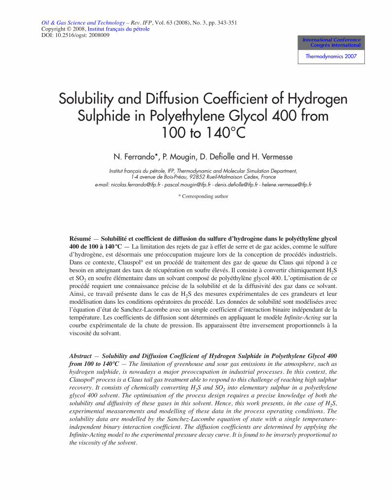
The experimental setup used in this work has been describedelsewhere [6, 7]. We only present here the main points of theapparatus schemed in Figure 1.

A 253.5-cm3 static cell made of Hastelloy is immerged ina LAUDA thermostatic liquid bath whose temperature fluc-tuation does not exceed 0.05 K. Two stirring rotors ensurethe homogeneity of liquid and vapour phases. Thermostatedtubing links this equilibrium cell to a 169.1-cm3 H2S storagetank immerged in a thermostatic liquid bath. Additional tub-ing is used to link the equilibrium cell either to a vacuum sys-tem to allow the degassing of the solvent, or to sodiumhydroxyl traps to securely clean the cell after each experi-ment. A Pt 100 probe measures temperature with an accuracyof 0.03 K. The pressure is measured with a HBM® 100 barpressure sensor with an accuracy of 0.015 MPa or with aHBM® 20 bar pressure sensor with an accuracy of0.0028 Mpa, depending on the experimental pressure range.

Hydrogen sulphide was provided by Air Liquid, with apurity of 99.7%. Polyethylene glycol 400 was provided byBASF. A Karl-Fisher titration indicated a water content of0.34 weight percent in the polymer. Hence, a dehydrationstep is included in the experimental procedure describedfurther.

1.2 Experimental Procedure

To measure solubility and estimate diffusion of H2S in PEG400, a three-step experimental procedure is performed.

The first step is the solvent dehydration in order to elimi-nate any traces of water dissolved in the commercial PEG400. The equilibrium cell is filled with a well-known amount

344

The Clauspol® process is licensed by Prosernat, 100% IFP subsidiary(http://www.prosernat.com), and is part of Advasulf™, a complete choiceof technologies to reach overall sulphur recovery up to 99.9+%.

C

B

PT

P T

PT

H2S

NaOH traps

Vacuum Solvent

C

A

BAB

Equilibrium cell

Thermostatic bath

Storage cell

Pressure sensor

Pt 100 probe

Figure 1

Experimental setup.

ogst07104_FOLIO 13/06/08 11:51 Page 344

of solvent (around 100 g). The temperature is then increasedto 120°C, and a vacuum is made in the cell for degassing it.At this temperature, the vapour pressure of polyethylene gly-col 400 is about 1 Pa according to the manufacturer. Hence,no loss of polymer is expected during this purification step.From the vacuum pressure in the cell, Pini, the residual dis-solved water is estimated in terms of molar fraction, xwater,from Raoult’s law:

(2)

where denotes the vapour pressure of water, computed fromthe DIPPR database [8]. Basically, this procedure allows oneto decrease the water content by up to 0.04 weight percent.

The diffusion acquisition is the second step of the mea-surement. The temperature of the thermostated bath isadjusted to the desired operating temperature. No agitation ofthe cell is performed in this measurement procedure. At theinitial time, a gas injection is performed and the pressuredecay is recorded during a three-day period. The preciseamount of hydrogen sulphide introduced, named n0

H2Sis

determined by a mass balance in the storage bottle before andafter the injection:

(3)

where V, T and P denote volume, temperature and pressure,respectively. R is the ideal gas constant (R = 8.31451J/mol/K), and Z the compressibility factor calculated fromthe Goodwin pure component equation of state [9]. Thesuperscripts initial and final denote the time before and afterthe gas injection, respectively. The subscript st refers to thestorage bottle. During the first two hours, the pressure in thecell is stored on a computer disk every five seconds. Afterthat, it is stored every five minutes. The final pressure decaycurve is exploited according to the model described further.

Finally, the third step of the experimental procedure is thehydrogen sulphur solubility measurements. Once the previ-ously described three-day period is ended, the agitation rotorsare started to completely reach thermodynamic equilibrium.The equilibrium pressure is noted, and a new gas injection isperformed. The hydrogen sulphur amount injected is alwayscalculated from the equation.

The amount of hydrogen sulphur dissolved in the solventafter each gas injection is determined by a mass balance:

nLH2S

= n0H2S

– nVH2S

(4)

where the superscripts L and V refer to the liquid and thevapour phases.

The amount of hydrogen sulphur in the vapour phase iscalculated from the relation:

2

0

( , ) ( , )

initial finalst st st

H S initial initial initial final final finalst st st st st st

V P Pn

R Z T P T Z T P T

⎛ ⎞= −⎜ ⎟

⋅ ⋅⎝ ⎠

( )

ini

waterwater

Px

P Tσ=

(5)

where the superscript eq refers to the thermodynamic equi-librium state, and the subscript cell refers to the equilib-rium cell. The vapour pressure of the solvent is assumed tobe negligible.

The volume of the vapour phase is known from a volumebalance:

VV = Vcell – VL (6)

The volume of the liquid phase is calculated from themass and density of the solvent, assuming that the variationin volume due to the dissolved gas is negligible:

(7)

where ms is the mass of the solvent and ρs its density at theoperating temperature. Preliminary work was done to deter-mine the density of the dehydrated polyethylene glycol 400used in this work according to the temperature:

(8)3 3( / ) 0.9037 ( ) 1.394 10s kg m T Kρ = − ⋅ + ⋅

L s

s

mV

ρ=

( , )

eq V

vap eqcell cellcell

P Vn

Z T P R T

⋅=

⋅ ⋅cell

N Ferrando et al. / Solubility and Diffusion Coefficient of Hydrogen Sulphide in Polyethylene Glycol 400 from 100 to 140°C 345

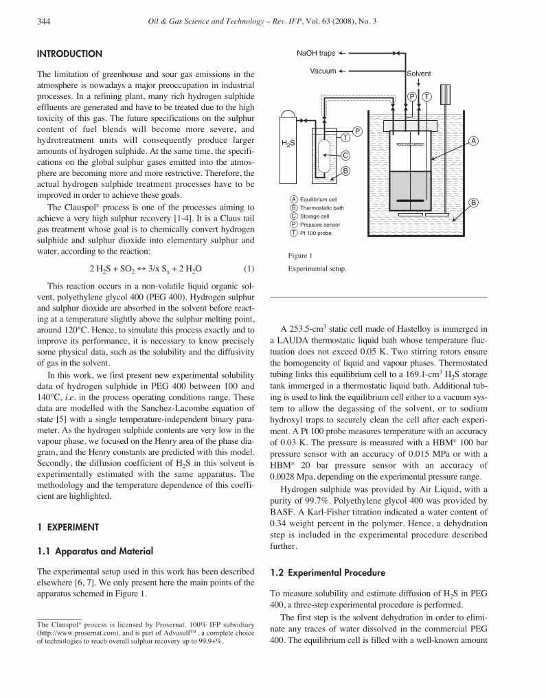
TABLE 1

Table of the experimental and calculated solubility of H2S in PEG 400

T P × H2S exp. × H2S calc. AAD1

K bar mol.frac. mol.frac. %

373.15 1.18 0.062 0.057 6.97

373.15 2.75 0.128 0.126 2.01

373.15 4.43 0.190 0.190 0.34

373.15 6.03 0.243 0.244 0.41

373.15 7.29 0.280 0.283 0.98

373.15 8.31 0.308 0.312 1.27

393.15 1.83 0.070 0.066 5.93

393.15 3.87 0.133 0.132 0.84

393.15 5.87 0.189 0.189 0.33

393.15 7.04 0.218 0.219 0.66

393.15 8.53 0.252 0.256 1.29

393.15 9.59 0.276 0.280 1.38

413.15 1.81 0.049 0.051 4.44

413.15 3.16 0.084 0.087 3.23

413.15 4.56 0.119 0.121 1.44

413.15 6.02 0.152 0.154 1.80

413.15 7.18 0.177 0.179 1.53

413.15 8.68 0.208 0.210 1.14

1 . .100

.

Exp value Calc valueAAD

Exp value

−= ⋅

ogst07104_FOLIO 13/06/08 11:51 Page 345

Oil & Gas Science and Technology – Rev. IFP, Vol. 63 (2008), No. 3

1.3 Experimental Results

Three isotherms are investigated: 100, 120 and 140°C. Foreach isotherm, the pressure decay is measured, and a series offive additional injections are carried out. Figure 2 shows thepressure decay experimental curve for each temperature.

Figure 3 plots the hydrogen solubility for each isothermfor pressure from about 1 to 10 bar. The experimental pointsare listed in Table 1. There are no other data of H2S solubilityin PEG 400 available in the literature. Hence, no direct com-parison or deviation estimation are possible. However, previ-ous experiments on H2S solubility in the same experimentalsetup, but in another solvent, have been reported in the litera-ture [10]. The reproducibility of these experiments was esti-mated at about 2.5%. We assume here the same uncertaintyfor our experimental points.

2 SOLUBILITY MODELLING

H2S solubility in PEG 400 is modelled with the Sanchez-Lacombe equation of state [5]:

(9)

where P–, T

–and ρ

–are the reduced pressure, temperature and

density given by:

(10)*

*

PvP

ε=

( ) 2111ln ρρρ −⎥

⎦

⎤⎢⎣

⎡⎟⎠

⎞⎜⎝

⎛ −+−−=r

TP

(11)

(12)

where ε*, v* and r are the microscopic parameters specific toeach pure component, corresponding to the interactionenergy between non-bonded molecular segments, the volumeof a lattice site, and the number of lattice sites occupied bythe molecule, respectively. For a mixture of c components,we adopt the following mixing rules:

(13)

(14)

with

(15)

(16)

(17)

where kij is an empirical binary interaction parameter.For polyethylene glycol 400, several sets of pure com-

ponent parameters, adjusted on PVT data, are available.We choose to use the parameters proposed by Sanchezand Panayiotou [11]. For hydrogen sulphide, two sets of

( ) ( )1/ 2* * * 1ij i j ijkε ε ε= −

( )* * *1

2ij i jv v v= +

r

rx iii =φ

* * * *

1 1

c c

i j ij iji j

v vε φφ ε= =

= ∑∑

∑=

=c

iiiivv

1

** φ

*rvρ ρ=

*

RTT

ε=

346

1.0

1.5

2.0

2.5

3.0

3.5

4.0

4.5

5.0

5.5

6.0

Time (s)

Pre

ssur

e (b

ar)

120°C140°C

100°C

0 50000 100000 150000 200000 250000

Figure 2

Pressure decay measurement during H2S diffusion in PEG400 at 100, 120 and 140°C.

0

2

4

6

8

10

12

Pre

ssur

e (b

ar)

This work: 100°CThis work: 120°CThis work: 140°CSanchez-Lacombemodel - kij = 0.0355

0.00 0.05 0.10 0.15 0.20 0.25 0.30 0.35 0.40

H2S molar fraction

Figure 3

Experimental and calculated solubility of H2S in PEG 400 at100, 120 and 140°C.

ogst07104_FOLIO 13/06/08 11:51 Page 346

parameters are found: one proposed by Kilpatrick and Chang[12] adjusted on experimental data of the pure componentproperties, and another determined from a correlation pro-posed by Gauter and Heidemann [13] based on the critical

properties. As shown in Figures 4 and 5, it is found that theset proposed by Kilpatrick and Chang naturally allows a bet-ter prediction of both vapour pressure (deviation about 3%)and saturated liquid density (deviation about 2%) of pureH2S. As a consequence, we choose to use this set of parame-ters for this compound. Finally, Table 2 resumes the pure-component Sanchez-Lacombe parameters used in this work.

TABLE 2

Pure-component Sanchez-Lacombe parameters of PEG 400 and H2S

Compound r ε* (J/mol) v* (m3/mol) Ref.

PEG 400 30.35 5495.55 1.1215.10-5 [11]

H2S 6.3540 3076.48 4.9080.10-6 [12]

Additionally, a binary interaction parameter is adjusted onour experimental data to reproduce them best. It is found thata single independent-temperature coefficient is sufficient toachieve a good accuracy. The optimal value is:

kH2S/PEG400 = 0.0355 (18)

The modelled data are plotted in Figure 3 and reported inTable 1. The average deviation between model and experi-ments is globally about 2.0%.

The model performed being accurate at predicting the sol-ubility data, it is used to calculate the Henry constant of H2Sin the solvent. By definition, the Henry constant is:

(19)

where ϕi denotes the fugacity coefficient of the solute in thevapour phase, and xi and yi its molar fraction in the liquid andthe vapour phases, respectively. As the solvent can beassumed to be non-volatile, the molar fraction of H2S in thevapour phase is equal to one. The fugacity coefficient can beextracted from the Sanchez-Lacombe equation of state. Itsanalytic expression is the following [14]:

(20)

with

(21)

(22)∑=

=c

iinn

1

RT

Pvz =

* *

* *

1

j ji in n

z nr v nrr v n nT

ρ εε

⎡ ⎤ ⎡ ⎤⎛ ⎞ ⎛ ⎞− ∂ ∂⎛ ⎞ ⎢ ⎥ ⎢ ⎥−⎜ ⎟ ⎜ ⎟⎜ ⎟ ∂ ∂⎢ ⎥ ⎢ ⎥⎝ ⎠ ⎝ ⎠ ⎝ ⎠

( )ln ln 2 ln 1i iz rT

ρϕ ρ

⎡ ⎤= − + − − − +⎢ ⎥

⎣ ⎦

⎣ ⎦ ⎣ ⎦

0limi

i ii x

i

P yH

x

ϕ→

⎛ ⎞= ⎜ ⎟

⎝ ⎠

N Ferrando et al. / Solubility and Diffusion Coefficient of Hydrogen Sulphide in Polyethylene Glycol 400 from 100 to 140°C 347

0

10

20

30

40

50

60

70

80

90

Temperature (K)

Vap

our

pres

sure

(ba

r)Experimental [8]Sanchez-Lacombe model with Kipatrickand Chang parametersSanchez-Lacombe model with Gauterand Heidemann parameters

180 200 220 240 260 280 300 320 340 360 380

Figure 4

Experimental and calculated vapour pressure of pure H2S.Experimental data are from the DIPPR database [8].Modelled data are calculated with the Sanchez-Lacombeequation of state with the Kilpatrick and Chang [12] and theGauter and Heidemann [13] parameter sets.

Temperature (K)

Experimental [8]Sanchez-Lacombe model with Kipatrickand Chang parametersSanchez-Lacombe model with Gauterand Heidemann parameters

180 200 220 240 260 280 300 320 340 360 3808000

13000

18000

23000

28000

Sat

urat

ed li

quid

den

sity

(m

ol/m

3 )

Figure 5

Experimental and calculated saturated liquid density of pureH2S. Experimental data are from the DIPPR database [8].Modelled data are calculated with the Sanchez-Lacombeequation of state with the Kilpatrick and Chang [12] and theGauter and Heidemann [13] parameter sets.

ogst07104_FOLIO 13/06/08 11:51 Page 347

Oil & Gas Science and Technology – Rev. IFP, Vol. 63 (2008), No. 3

(23)

Hence, the fugacity coefficient at infinite dilution (i.e.when the concentration of the solute leads to zero) is givenby:

(24)

where, with the chosen mixing rules:

(25)

(26)

(27)

(28)

(29)

The saturated molar volume of the pure solvent vσs is com-

puted from the equation of state. Finally, the Henry constantsof hydrogen sulphide in polyethylene glycol for the threetemperatures investigated are given in Table 3. According tothe uncertainty of the experimental data and the precision ofthe model, we assume an uncertainty of about 5% for theseHenry constant values.

TABLE 3

Henry constant of H2S in PEG 400 at 100, 120 and 140°C

T (K) H (bar/mol.frac.)

373.15 19.59

393.15 26.15

413.15 33.65

3 DIFFUSION COEFFICIENT MODELLING

The diffusion coefficient is determined with an inverse prob-lem methodology, in which the experimental data can be

RT

vPz ss

σσ

=∞

*s

RTT

ε=

∞

σρ

s

ss

v

vr *

=∞

( )( ) ( )* * * * * **

1 11

2 s i is s i i s is

k v v r v vv

ε ε⎤⎞ ⎡ ⎤− + − − +⎟⎥ ⎣ ⎦⎠⎦

** *

* * *

1lim 2 i s s

i s s

nrr v

n vε

εε ε

⎡ ⎤ ⎡∂ ⎛= − +⎢ ⎥ ⎜⎢∂ ⎝⎣⎣ ⎦

( )[ ]***

*

*

1lim isi

si

vvrvn

v

v

nr+−=⎥

⎦

⎤⎢⎣

⎡

∂∂

1 1

* *

* *0 0

1lim limn n

s i i

z nr v nrr v n nT

ρ εε

∞∞

∞→ →

⎛ ⎞ ⎡ ⎤ ⎡ ⎤− ∂ ∂−⎜ ⎟ ⎢ ⎥ ⎢ ⎥∂ ∂⎝ ⎠ ⎣ ⎦ ⎣ ⎦

( )ln ln 2 ln 1i iz rT

ρϕ ρ

∞∞∞ ∞

∞

⎡ ⎤= − + − − − +⎢ ⎥

⎢ ⎥⎣ ⎦

∑=

=c

iii rxr

1

reproduced on the basis of unknown parameters. In our case,the unknown parameter is the diffusion coefficient, and theexperimental data are the pressure decay curve. The modelused to reproduce this curve is the so-called Infinite-Actingmodel, largely described by Sheikha et al. [15] in their bibli-ographic review of diffusion coefficient determinationmethodologies. The assumptions of the methodology are thefollowing: the system is non-reactive, isothermal conditionsare assumed throughout the pressure decay experiment, thesolvent is non-volatile, the diffusion coefficient is constant,there is only a diffusion phenomenon which follows Fick’ssecond law, the Henry law can be applied to the gas-liquidequilibrium at the interface, and the liquid phase is a semi-infinite medium.

Following Fick’s second law:

(30)

where D is the diffusion coefficient, and C(z,t) the dissolvedgas concentration in the liquid phase at the depth z in the liq-uid phase (origin is taken at the gas-liquid interface) and atthe time t.

A mass balance at the interface (z = 0) gives:

(31)

where Vg is the volume of the vapour phase, calculated fromthe equation, Cg(t) the gas concentration in the vapour phase,and S the surface of the gas-liquid interface known from thegeometry of the equilibrium cell.

The Henry law at the gas-liquid interface is:

(32)

where v– is the molar volume of the liquid phase, assumed tobe equal to the molar volume of the solvent (as for the solu-bility data calculation methodology, the variation in volumedue to the dissolved gas is neglected).

With the relation:

P = Z (T, P) Cg (t) RT (33)

the Henry law expression is equivalent to:

Cg (t) = α · C (0, t) (34)with

(35)

This differential equations system is solved using theLaplace transforms. In the mathematical resolution, it isassumed that the α parameter does not depend on the time.

( , )Hv

Z T P RTα =

(0, )

PH

v C t=

⋅

0

),()(

=

⎟⎠

⎞⎜⎝

⎛

∂∂

−=∂

∂−

z

gg z

tzCSD

t

tCV

ttzC

z

tzCD

∂∂

=∂

∂ ),(),(2

2

348

ogst07104_FOLIO 13/06/08 11:51 Page 348

N Ferrando et al. / Solubility and Diffusion Coefficient of Hydrogen Sulphide in Polyethylene Glycol 400 from 100 to 140°C 349

Because the pressure difference between the initial and thefinal time of the pressure decay curve is relatively small(3 bar at max.), this assumption is realistic. Rigorously, afterthe initial degassing process, the pressure in the cell is equalto the vapour pressure of the solvent Pb. Because of theextremely low volatility of PEG 400, it is in fact the vapourpressure of the traces of water in this solvent. Therefore, it isnecessary to work with relative pressures. Finally, the expres-sion of pressure as a function of time is:

(36)

where P(0) is the pressure just after the gas introduction, andwith:

(37)

and L is the height of the vapour phase, calculated with:

(38)

At this step, the methodology consists of fitting the coeffi-cient diffusion in order to reproduce well the experimentalpressure decay curve. However, due to the non-linearity ofthe equation, the adjustment method is complex. Thus, weshould modify equation to obtain a linear form. Moreover, itis important to note that this Infinite-Acting model gives foran infinite time a pressure equal to zero and not, as we canexpect, equal to the equilibrium pressure. Hence, this modelcannot be used in the whole range of time, and has to beemployed only at the beginning of the pressure decay curve.The linearisation of equation must allow one to easily deter-mine the validity range of the model.

In this way, we use the methodology proposed by Sheikhaet al. [16], consisting of using a development of the erfcfunction. Indeed, following the mathematical form proposedby Abramovitch [17]:

(39)

with

(40)

and a1 = 0.3480242, a2 = _0.0958798, a3 = 0.7478556, a4 =0.47047, ⎪ε⎪ < 2.5.10-5. Reporting that in equation, we find:

(41)

Such an equation can be reformulated in:

(42)3 2 0a b c dφ φ φ+ + + =

[ ] [ ]( )3 2

3 2 1

( ) ( , (0))( ) ( ) ( )

(0) ( , ( ))b

b

P t P Z T Pa a a

P P Z T P tβ φ β φ β φ

−⋅ = + +

−

4

1( )

1x

a xβ =

+

[ ] [ ]( )3 2 23 2 1( ) ( ) ( ) ( ) exp( )erfc x a x a x a x xβ β β ε= + + − +

gVLS

=

2 2

DtL

φα

=

( ) ( )2( ) ( , ( ))exp

(0) ( , (0))b

b

P t P Z T P terfc

P P Z T Pφ φ

−= ⋅

−

with:

(43)

(44)

(45)

(46)

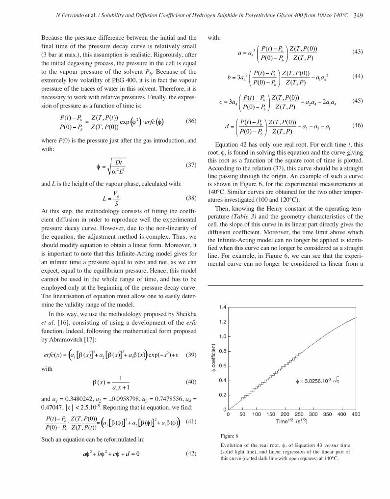
Equation 42 has only one real root. For each time t, thisroot, φ, is found in solving this equation and the curve givingthis root as a function of the square root of time is plotted.According to the relation (37), this curve should be a straightline passing through the origin. An example of such a curveis shown in Figure 6, for the experimental measurements at140°C. Similar curves are obtained for the two other temper-atures investigated (100 and 120°C).

Then, knowing the Henry constant at the operating tem-perature (Table 3) and the geometry characteristics of thecell, the slope of this curve in its linear part directly gives thediffusion coefficient. Moreover, the time limit above whichthe Infinite-Acting model can no longer be applied is identi-fied when this curve can no longer be considered as a straightline. For example, in Figure 6, we can see that the experi-mental curve can no longer be considered as linear from a

3 2 1

( ) ( , (0))(0) ( , )

b

b

P t P Z T Pd a a a

P P Z T P

⎛ ⎞−= − − −⎜ ⎟

−⎝ ⎠

4 2 4 1 4

( ) ( , (0))3 2

(0) ( , )b

b

P t P Z T Pc a a a a a

P P Z T P

⎛ ⎞−= − −⎜ ⎟

−⎝ ⎠

2 24 1 4

( ) ( , (0))3

(0) ( , )b

b

P t P Z T Pb a a a

P P Z T P

⎛ ⎞−= −⎜ ⎟

−⎝ ⎠

34

( ) ( , (0))(0) ( , )

b

b

P t P Z T Pa a

P P Z T P

⎛ ⎞−= ⎜ ⎟

−⎝ ⎠

0

0.2

0.4

0.6

0.8

1.0

1.2

1.4

φ co

effic

ient

Time1/2 (s1/2)0 50 100 150 200 250 300 350 400 450

φ = 3.0256.10-3 . t

Figure 6

Evolution of the real root, φ, of Equation 43 versus time(solid light line), and linear regression of the linear part ofthis curve (dotted dark line with open squares) at 140°C.

ogst07104_FOLIO 13/06/08 11:51 Page 349

square root of time of about 350 s1/2. This example showsthat we consider a decay of pressure by a factor of around2 to deduce the diffusion coefficient. Hence, not only the ini-tial slope of the pressure decay curve is used. Moreover, inthis example, after 34 hours the curve still follows Fick’slaw, and no convection phenomenon is noticed. For eachtemperature, the calculated diffusion coefficient is sum-marised in Table 4. With this methodology, the diffusioncoefficient appears to be very sensitive to the Henry constantvalue. According to the uncertainty of our previously deter-mined Henry constants, we assume an uncertainty of about10% in the diffusion coefficient. It is also important to notethat according to the large number of assumptions and thesimplification in the mathematical treatment of the curve,these values cannot be considered as rigorous measurementsof the diffusion coefficient, but only as estimations.

TABLE 4

Diffusion coefficient of H2S in PEG 400 at 100, 120 and 140°C

T (K) 109 D (m2/s)

373.15 1.6853

393.15 2.2270

415.15 3.6214

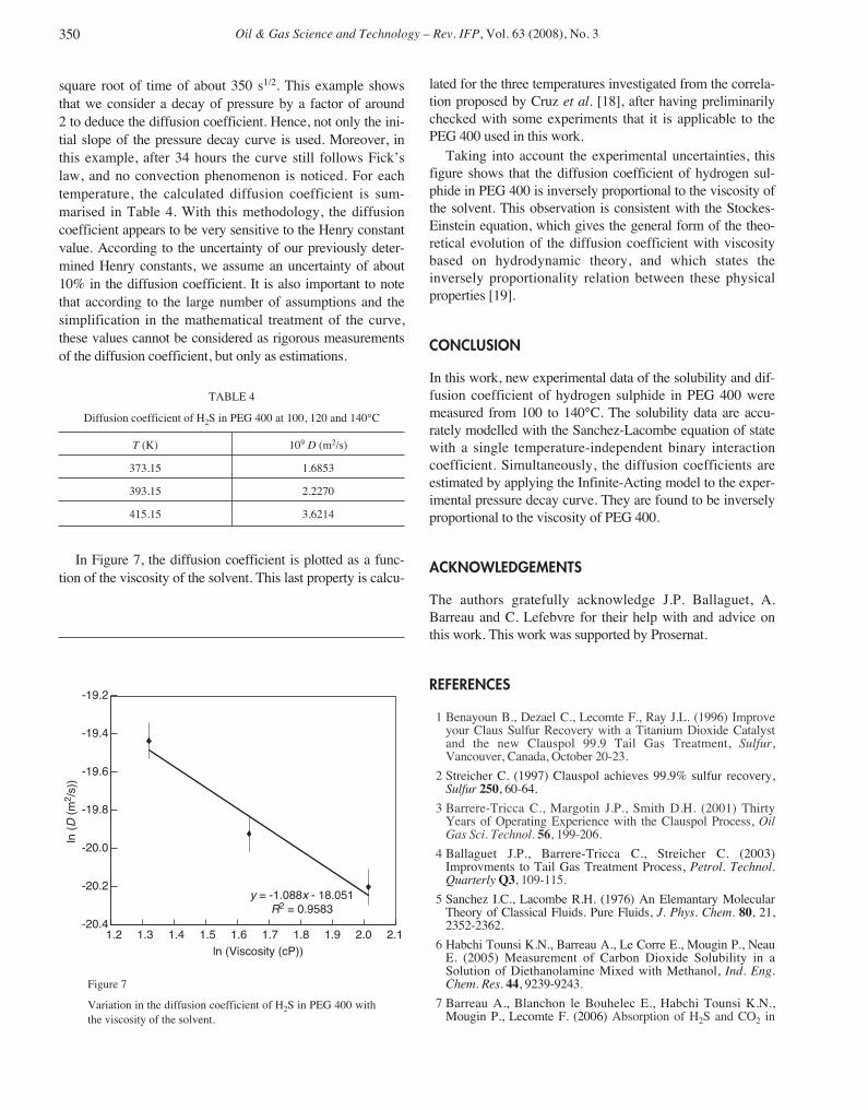
In Figure 7, the diffusion coefficient is plotted as a func-tion of the viscosity of the solvent. This last property is calcu-

lated for the three temperatures investigated from the correla-tion proposed by Cruz et al. [18], after having preliminarilychecked with some experiments that it is applicable to thePEG 400 used in this work.

Taking into account the experimental uncertainties, thisfigure shows that the diffusion coefficient of hydrogen sul-phide in PEG 400 is inversely proportional to the viscosity ofthe solvent. This observation is consistent with the Stockes-Einstein equation, which gives the general form of the theo-retical evolution of the diffusion coefficient with viscositybased on hydrodynamic theory, and which states theinversely proportionality relation between these physicalproperties [19].

CONCLUSION

In this work, new experimental data of the solubility and dif-fusion coefficient of hydrogen sulphide in PEG 400 weremeasured from 100 to 140°C. The solubility data are accu-rately modelled with the Sanchez-Lacombe equation of statewith a single temperature-independent binary interactioncoefficient. Simultaneously, the diffusion coefficients areestimated by applying the Infinite-Acting model to the exper-imental pressure decay curve. They are found to be inverselyproportional to the viscosity of PEG 400.

ACKNOWLEDGEMENTS

The authors gratefully acknowledge J.P. Ballaguet, A.Barreau and C. Lefebvre for their help with and advice onthis work. This work was supported by Prosernat.

REFERENCES

1 Benayoun B., Dezael C., Lecomte F., Ray J.L. (1996) Improveyour Claus Sulfur Recovery with a Titanium Dioxide Catalystand the new Clauspol 99.9 Tail Gas Treatment, Sulfur,Vancouver, Canada, October 20-23.

2 Streicher C. (1997) Clauspol achieves 99.9% sulfur recovery,Sulfur 250, 60-64.

3 Barrere-Tricca C., Margotin J.P., Smith D.H. (2001) ThirtyYears of Operating Experience with the Clauspol Process, OilGas Sci. Technol. 56, 199-206.

4 Ballaguet J.P., Barrere-Tricca C., Streicher C. (2003)Improvments to Tail Gas Treatment Process, Petrol. Technol.Quarterly Q3, 109-115.

5 Sanchez I.C., Lacombe R.H. (1976) An Elemantary MolecularTheory of Classical Fluids. Pure Fluids, J. Phys. Chem. 80, 21,2352-2362.

6 Habchi Tounsi K.N., Barreau A., Le Corre E., Mougin P., NeauE. (2005) Measurement of Carbon Dioxide Solubility in aSolution of Diethanolamine Mixed with Methanol, Ind. Eng.Chem. Res. 44, 9239-9243.

7 Barreau A., Blanchon le Bouhelec E., Habchi Tounsi K.N.,Mougin P., Lecomte F. (2006) Absorption of H2S and CO2 in

Oil & Gas Science and Technology – Rev. IFP, Vol. 63 (2008), No. 3350

-20.4

-20.2

-20.0

-19.8

-19.6

-19.4

-19.2

ln (Viscosity (cP))

ln (

D (

m2 /

s))

y = -1.088x - 18.051R2 = 0.9583

1.2 1.3 1.4 1.5 1.6 1.7 1.8 1.9 2.0 2.1

Figure 7

Variation in the diffusion coefficient of H2S in PEG 400 withthe viscosity of the solvent.

ogst07104_FOLIO 13/06/08 11:51 Page 350

N Ferrando et al. / Solubility and Diffusion Coefficient of Hydrogen Sulphide in Polyethylene Glycol 400 from 100 to 140°C 351

Alkanolamine Aqueous Solution: Experimental Data andModelling with the Electrolyte-NRTL Model, Oil Gas Sci.Technol. 61, 345-361.

8 BYU DIPPR 801 (2005) Thermophysical properties databasepublic release, January 2005.

9 Goodwin R.D. (1983) Hydrogen Sulfide ProvisionalThermophysical Properties from 188 to 700 K at Pressures to 75MPa, NBSIR 83-1694, National Bureau of Standards.

10 Blanchon le Bouhelec E., Tribouillois E. (2006) Contribution àla thermodynamique de l’absorption des gaz acides H2S et CO2dans les solvants eau-alcanolamine-méthanol : mesures expéri-mentales et modélisation, Thèse de doctorat de l’InstitutNational Polytechnique de Lorraine.

11 Sanchez I.C., Panayiotou C.G. (1994) Equation of StateThermodynamics of Polymer and Related Solutions, in Modelsfor Thermodynamic and Phase Equilibria calculations, Sandler S.I. (Ed.), New-York, p. 207.

12 Kilpatrick P.K., Chang S.H. (1986) Saturated Phase Equilibriaand Parameter Estimation of Pure Fluids with Two Lattice-GasModels, Fluid Phase Equilibria 30, 49-56.

13 Gauter K., Heidemann R.A. (2000) A Proposal for Parametrizingthe Sanchez-Lacombe Equation of State, Ind. Eng. Chem. Res.39, 1115-1117.

14 Neau E. (2002) A consistent method for phase equilibrium cal-culation using the Sanchez-Lacombe lattice-fluid equation ofstate, Fluid Phase Equilibr. 203, 133-140.

15 Sheikha H., Pooladi-Darvish M., Mehrotra A.K. (2005)Development of graphical methods for estimating the diffusivitycoefficient of gases in bitumen from pressure-decay data, Energ.Fuel. 19, 2041-2049.

16 Sheikha H., Mehrotra A.K., Pooladi-Darvish M. (2006) Aninverse solution methodology for estimating the diffusion coeffi-cient of gases in Athabasca bitumen from pressure decay data, J.Petrol. Sci. Eng. 53, 189-202.

17 Abramowitz M., Stegun I.A. (1970) Handbook of mathematicalfunctions with formulas, graphs and mathematical tables, NBS,Appl. Math. 55, 1020.

18 Cruz M.S., Chumpitaz L.D.A., Alves J.G.L.F., Meirelles A.J.A.(2000) Kinematic Viscosities of Poly(ethylene glycols), J. Chem.Eng. Data 45, 61-63.

19 Reid R.C., Prausnitz J.M., Poling B.E. (1987) The Properties ofGases and Liquids, McGraw-Hill, Inc., 4th ed.

Final manuscript received in November 2007Published online in May 2008

Copyright © 2008 Institut français du pétrolePermission to make digital or hard copies of part or all of this work for personal or classroom use is granted without fee provided that copies are not madeor distributed for profit or commercial advantage and that copies bear this notice and the full citation on the first page. Copyrights for components of thiswork owned by others than IFP must be honored. Abstracting with credit is permitted. To copy otherwise, to republish, to post on servers, or to redistributeto lists, requires prior specific permission and/or a fee: Request permission from Documentation, Institut français du pétrole, fax. +33 1 47 52 70 78, or revueogst@ifp.fr.

ogst07104_FOLIO 13/06/08 11:51 Page 351