solving nonlinear equations - ucsc directory of … nonlinear equations jijianfan department of...

Solving Nonlinear Equations

Jijian Fan

Department of EconomicsUniversity of California, Santa Cruz

Oct 13 2014

Overview

NUMERICALLY solving nonlinear equation

f(x) = 0

Four methodsBisectionFunction iterationNewton’sQuasi-Newton

Motivation

Linear equation can be solved analyticallyAx = b ⇒ x = A−1bMethods such as L-U factorization, Gaussian elimination,etc

However, nonlinear equation might not be explicitly solvede.g. f(x) = x−0.8 + 2x0.5 − 3 = 0Numerical methods

Numerical methods

"Continuous" means 1, 1.001, . . . , 1.999, 2"Equality" means 1 = 1.0003

Figure 1 : A "continuous" function in computer

Bisection Method

Based on Intermediate Value TheoremStart with a bounded interval [a, b] such that f(a)f(b) < 0

Sample codewhile (b-a)>tol;

if sign(f((a+b)/2)) == sign(f(a))a= (a+b)/2;

elseb= (a+b)/2;

endx=a;

Bisection Method

AdvantageReliable: always finds the rootLEAST requirements on functional properties

DisadvantageUnivariate f : R 7→ RSlow log(n)

Function Iteration

Solve for fixed point x = g(x)f(x) = 0⇔ x = g(x) = x− f(x)

Start with an initial guess x(0) s.t. ||g′(x(0))|| < 1

Sample codex=x0;y=g(x);while norm(y-x)>tol;

x=y;y=g(x);

end

Function Iteration

AdvantageCould be multivariate f : Rn 7→ Rn

Easy-coding

DisadvantageNot reliable: require differentiability, andInitial x(0) should be sufficiently close to a fixed point x∗Only applicable to downward-crossing fixed point||g′(x∗)|| < 1Worth trying even if one or more condition fails

Function Iteration: Extension

Value Function Iteration (VFI)

V(k) = maxk′{u(c) + βV(k′)}

k′ = f(k)− c+ (1− δ)k

Rewrite as

V(k) = maxk′{u(f(k) + (1− δ)k− k′) + βV(k′)}

Function Iteration: Extension

Make a grid of kMake an initial guess V0(k) for each kUpdating: for every k, update

Vi+1(k) = maxk′{u(f(k) + (1− δ)k− k′) + βVi(k′)}

by trying each possible k′

Repeat updatingUntil Vi+1(k) is close enough to Vi(k)

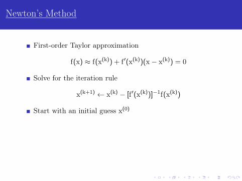
Newton’s Method

First-order Taylor approximation

f(x) ≈ f(x(k)) + f ′(x(k))(x− x(k)) = 0

Solve for the iteration rule

x(k+1) ← x(k) − [f ′(x(k))]−1f(x(k))

Start with an initial guess x(0)

Pseudo-codefor iter=1:maxiter

[ fval fjac ]=f(x);x = x - fjac \ fval;if norm(fval) < tol, break, end

end

Newton’s Method: Calculate the Jacobian Matrix

How to calculate the Jacobian Matrix

f ′(x) =

∂f1/∂x1 ∂f1/∂x2 . . . ∂f1/∂xn∂f2/∂x1 ∂f2/∂x2 . . . ∂f2/∂xn

......

. . ....

∂fn/∂x1 ∂fn/∂x2 . . . ∂fn/∂xn

Analytical derivativesNumerical derivatives


Analytical derivatives example: Cournot duopoly model

P(q) = q−1/η

Ci(qi) =12ciq2

i

maxqi

πi(q1, q2) = P(q1 + q2)qi − Ci(qi)

F.O.C.∂πi

∂qi= P(q1 + q2) + P′(q1 + q2)qi − C′i(qi) = 0

Let

~f(~q) =

[∂π1∂q1

(q1, q2)∂π2∂q2

(q1, q2)

]Solve

~f(~q) = ~0


Note that∂fi∂xj≡ ∂2πi

∂qj∂qi

function [fval,fjac]=f(q)c=[0.6,0.8]; eta=1.6; e=-1/eta;fval=sum(q)ˆe + e*sum(q)ˆ(e-1)*q-diag(c)*q;fjac=e*sum(q)ˆ(e-1)*ones(2,2)+e*sum(q)ˆ(e-1)*eye(2)+ (e-1)*e*sum(q)ˆ(e-2)*q*[1 1]-diag(c);

end


Numerical derivatives

f ′(x) ≈ f(x+ ε)− f(x)(x+ ε)− x

=f(x+ ε)− f(x)

ε

Centered finite difference approximation

f ′(x) ≈ f(x+ ε)− f(x− ε)(x+ ε)− (x− ε)

=f(x+ ε)− f(x− ε)

2ε


For multivariate case, let

ε =

0...0ε0...0

Quasi-Newton Methods

Calculating f ′(x) and taking inverse isSlowInefficient

GoalFind a proper approximation of f ′(x) or (f ′(x))−1

Update this approximation in a more efficient wayMethods

Secant methodBroyden’s method

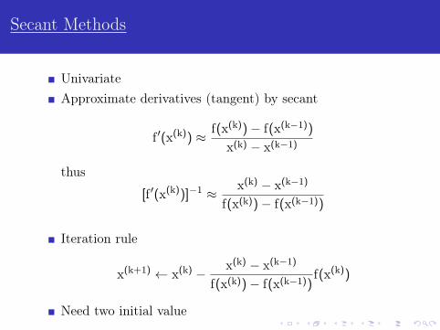
Secant Methods

UnivariateApproximate derivatives (tangent) by secant

f ′(x(k)) ≈ f(x(k))− f(x(k−1))

x(k) − x(k−1)

thus

[f ′(x(k))]−1 ≈ x(k) − x(k−1)

f(x(k))− f(x(k−1))

Iteration rule

x(k+1) ← x(k) − x(k) − x(k−1)

f(x(k))− f(x(k−1))f(x(k))

Need two initial value

Broyden’s Methods

Generalized secant method for multivariateDenote A(k) as the Jacobian approximant of f at x = x(k)

Newton iteration

x(k+1) ← x(k) − (A(k))−1f(x(k))

Secant condition must hold at x(k+1)

f(x(k+1))− f(x(k)) = A(k+1)(x(k+1) − x(k))

Broyden’s Methods

Choose A(k+1) that minimizes Frobenius norm

minA(k+1)

||A(k+1)−A(k)|| =√

trace((A(k+1) −A(k))>(A(k+1) −A(k)))

subject to

f(x(k+1))− f(x(k)) = A(k+1)(x(k+1) − x(k))

Solve for A(k+1)

A(k+1) ← A(k) + [f(x(k+1))− f(x(k))−A(k)d(k)]d(k)>

d(k)>d(k)

whered(k) = x(k+1) − x(k)

Broyden’s Methods

Improvement: directly update B(k) ≡ (A(k))−1

Sherman-Morrison formula

(A+ uv>)−1 = A−1 +1

1+ u>A−1vA−1uv>A−1

Iteration rule

B(k+1) ← B(k) +(d(k) − u(k))d(k)>B(k)

d(k)>u(k)

where

d(k) = x(k+1) − x(k) u(k) = B(k)[f(x(k+1))− f(x(k))]

Broyden’s Methods

Pseudo-code

Choose initial xCalculate initial B (usually B = f ′−1(x))loop

update xif f(x) is close enough to 0 then breakupdate B

end

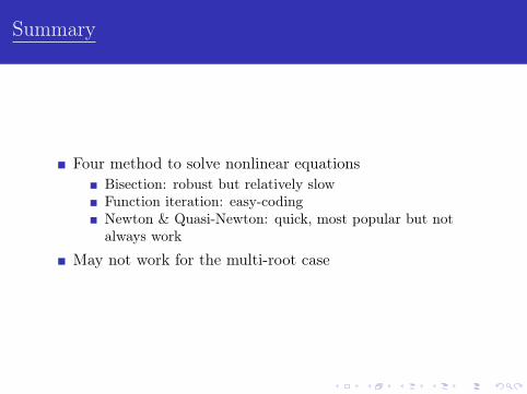
Summary

Four method to solve nonlinear equationsBisection: robust but relatively slowFunction iteration: easy-codingNewton & Quasi-Newton: quick, most popular but notalways work

May not work for the multi-root case

solving nonlinear equations - ucsc directory of … nonlinear equations jijianfan department of...

Documents