solving simultaneous nonlinear equations -...
TRANSCRIPT
Solving Simultaneous
Nonlinear Equations
Substitutive Iteration and
Graphical Method
SELİS ÖNEL, PhD

SelisÖnel© 2
Quotes of the Day:
Keep Moving Forward
"Every worthwhile accomplishment, big or little, has its stages of drudgery and triumph; a beginning, a struggle and a victory." Ghandi
"The price of success is hard work,
dedication to the job at hand, and the determination that whether we win or lose, we have applied the best of ourselves to the task at hand."
Vince Lombardi
• An iterative technique to solve system of multivariate nonlinear equations
• Plotting 2.5D and 3D plots of multivariate functions
What are we going to learn
today?
SelisÖnel© 3

SelisÖnel© 4
Nonlinear Functions of Several Variables
System with two nonlinear functions and two variables
z=f(x1,x2) and z=g(x1,x2)
Problem is more difficult to solve for more variables f(x1,x2,x3,…,xn)

SelisÖnel© 5
Nonlinear Functions of Several Variables
To find a zero of the system, find the intersection of the curves:
f(x1,x2)=0 and g(x1,x2)=0
ex: f(x,y)=x2+y2-1 and g(x,y)=x2-y
Use all the information about the problem to find the region where the curves may intersect SO…???

SelisÖnel© 6
Nonlinear Functions of Several Variables
Plot a 2-D or 3-D figure of the functions in MATLAB® !

SelisÖnel© 7
2-D Graphs >> x=linspace(0,2);
% linspace generates a row vector of 100 linearly
% equally spaced points between x1 and x2
>> y=x.*exp(-x);
>> plot(y)
% plots y versus their index
0 10 20 30 40 50 60 70 80 90 1000
0.05
0.1
0.15
0.2
0.25
0.3
0.35
0.4
SelisÖnel© 8
0 0.2 0.4 0.6 0.8 1 1.2 1.4 1.6 1.8 20
0.05
0.1
0.15
0.2
0.25
0.3
0.35
0.4
x
y
y=xe-x
anywhere
(0.36,0.25)
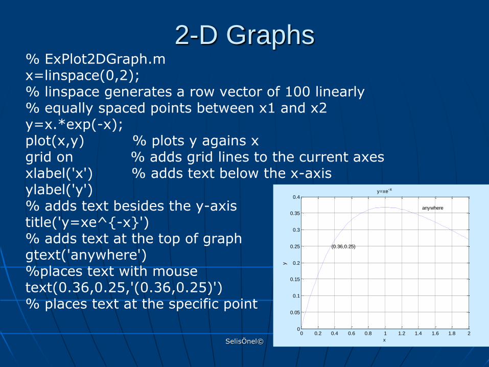
2-D Graphs % ExPlot2DGraph.m x=linspace(0,2); % linspace generates a row vector of 100 linearly % equally spaced points between x1 and x2 y=x.*exp(-x); plot(x,y) % plots y agains x grid on % adds grid lines to the current axes xlabel('x') % adds text below the x-axis ylabel('y') % adds text besides the y-axis title('y=xe^{-x}') % adds text at the top of graph gtext('anywhere') %places text with mouse text(0.36,0.25,'(0.36,0.25)') % places text at the specific point

SelisÖnel© 9
2-D Graphs % ExPlot.m: This program draws a graph of sin(x) and cos(x) % where
0 <= x <= 3.14 angle=-pi:0.1:pi; % Create array xcomp=cos(angle); % Create array plot(angle,xcomp,'r:'); % Plot using dots(:) with red(r) hold on % Add another plot on the same graph ycomp=sin(angle); % Create array plot(angle,ycomp,'b-x'); % Plot using lines(-) and the symbol x % at each data point with blue(b) grid on xlabel('Angle in degrees'); ylabel('x and y components'); legend('cos{\theta}','sin{\theta}',2) gtext('cos(x)'); gtext('sin(x)'); % Display mouse-movable text
-4 -3 -2 -1 0 1 2 3 4-1
-0.8
-0.6
-0.4
-0.2
0
0.2
0.4
0.6
0.8
1
Angle in degrees
x a
nd y
com
ponents
cos(x)
sin(x)
cos
sin

SelisÖnel© 10
2-D Graphs: Other Commands
More than one function can be plotted on one graph:
>>plot(x,X.*exp(-x),’.’,x,x*sin(x),’-.’) More than one graph can be shown in different
frames >>subplot(2,1,1), plot(x,x.*cos(x)) >>subplot(2,1,2), plot(x,x.*sin(x) Axis limits can be seen or modified >>axis >>axis([0,1.5,0,1.5]) Figure window can be cleared >>clf

SelisÖnel© 11
2-D Graphs: Other Commands
Comet like trajectory of the function
>> shg, comet(x,y)
% shg brings up the current graphic window
By using figure(n) command, it is possible to use more than one graphic window, n: positive integer
Another easy way to plot a function:
>>fplot(x*)

SelisÖnel© 12
2-D Graphs: fplot
Another easy way to plot a function: fplot
fplot(@humps,[0 1])
fplot(@(x)[tan(x),sin(x),cos(x)], 2*pi*[-1 1 -1 1])
fplot(@(x) sin(1./x), [0.01 0.1], 1e-3)
f = @(x,n)abs(exp(-1j*x*(0:n-1))*ones(n,1));
fplot(@(x)f(x,10),[0 2*pi])
>> fplot('x*exp(-x)',[0,2])
0 0.2 0.4 0.6 0.8 1 1.2 1.4 1.6 1.8 20
0.05
0.1
0.15
0.2
0.25
0.3
0.35
0.4

SelisÖnel© 13
2-D Graphs: Other Commands
semilogx(x,y)
% semilogarithmic plot
% log scale x-axis
semilogy(x,y)
% log scale y-axis
loglog(x,y)
% log scale x- and y-axis
0 10 20 30 40 50 60 70 80 90 10010
-50
10-40
10-30
10-20
10-10
100
x=0:100; semilogy(x,x.*exp(-x)), grid
100
101
102
10-50
10-40
10-30
10-20
10-10
100
x=0:100; loglog(x,x.*exp(-x)), grid
SelisÖnel© 14
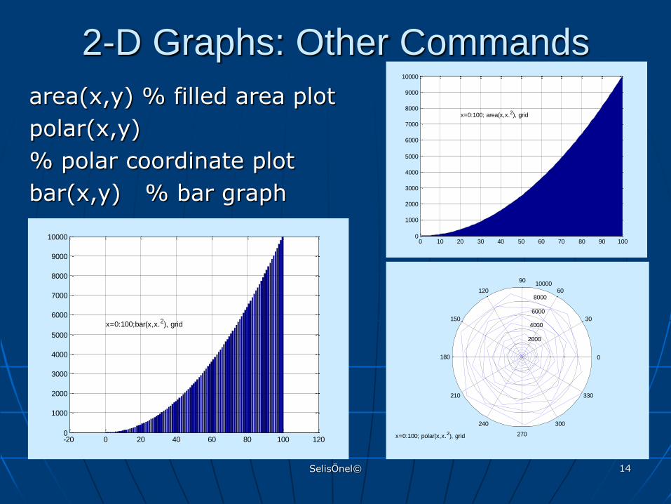
2-D Graphs: Other Commands
area(x,y) % filled area plot
polar(x,y)
% polar coordinate plot
bar(x,y) % bar graph
0 10 20 30 40 50 60 70 80 90 1000
1000
2000
3000
4000
5000
6000
7000
8000
9000
10000
x=0:100; area(x,x.2), grid
2000
4000
6000
8000
10000
30
210
60
240
90
270
120
300
150
330
180 0
x=0:100; polar(x,x.2), grid-20 0 20 40 60 80 100 1200
1000
2000
3000
4000
5000
6000
7000
8000
9000
10000
x=0:100;bar(x,x.2), grid

SelisÖnel© 15
3-D Graphs
% ExPlot3DGraph.m
t=0:0.01:3*pi;
plot3(t,sin(t),cos(t))
xlabel('x'),
ylabel('sin(t)'),
zlabel('cos(t)')
grid 0
24
68
10
-1
-0.5
0
0.5
1-1
-0.5
0
0.5
1
xsin(t)
cos(t
)

SelisÖnel© 16
3-D Graphs: Surfaces % ExPlot3DGraphSurface.m
[x,y]=meshgrid(-pi:pi/10:pi, -pi:pi/10:pi);
z=cos(x).*cos(y);
figure(1), mesh(x,y,z)
figure(2), surf(x,y,z)
figure(3), surf(x,y,z), view(30,60)
-4
-2
0
2
4
-4
-2
0
2
4-1
-0.5
0
0.5
1
-4
-2
0
2
4
-4
-2
0
2
4-1
-0.5
0
0.5
1
-4
-2
0
2
4 -4
-2
0
2
4
-1
0
1
SelisÖnel© 17
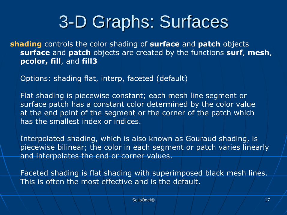
3-D Graphs: Surfaces shading controls the color shading of surface and patch objects surface and patch objects are created by the functions surf, mesh, pcolor, fill, and fill3 Options: shading flat, interp, faceted (default) Flat shading is piecewise constant; each mesh line segment or surface patch has a constant color determined by the color value at the end point of the segment or the corner of the patch which has the smallest index or indices. Interpolated shading, which is also known as Gouraud shading, is piecewise bilinear; the color in each segment or patch varies linearly and interpolates the end or corner values. Faceted shading is flat shading with superimposed black mesh lines. This is often the most effective and is the default.
SelisÖnel© 18
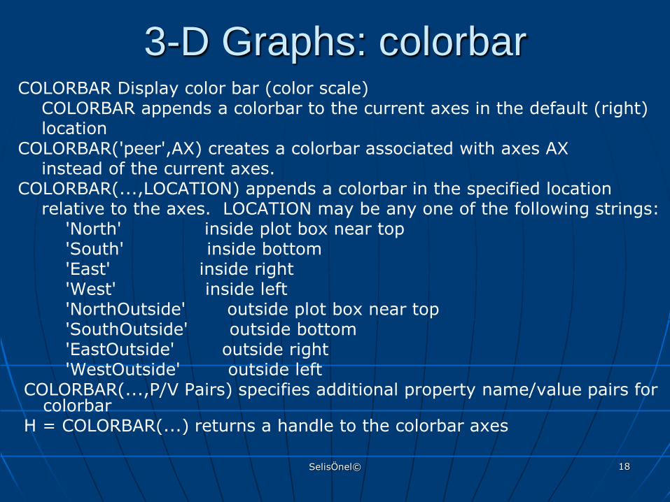
3-D Graphs: colorbar COLORBAR Display color bar (color scale) COLORBAR appends a colorbar to the current axes in the default (right) location COLORBAR('peer',AX) creates a colorbar associated with axes AX instead of the current axes. COLORBAR(...,LOCATION) appends a colorbar in the specified location relative to the axes. LOCATION may be any one of the following strings: 'North' inside plot box near top 'South' inside bottom 'East' inside right 'West' inside left 'NorthOutside' outside plot box near top 'SouthOutside' outside bottom 'EastOutside' outside right 'WestOutside' outside left COLORBAR(...,P/V Pairs) specifies additional property name/value pairs for
colorbar H = COLORBAR(...) returns a handle to the colorbar axes

SelisÖnel© 19
MATLAB® Plotting Command: surf
Plots 3-D surface surf(x,y,z,c) plots the colored parametric
surface defined by four matrix arguments. • The view point is specified by view. The axis labels
are determined by the range of X, Y and Z, or by the current setting of axis
• The color scaling is determined by the range of C, or by the current setting of caxis.
• The scaled color values are used as indices into the current colormap
• The shading model is set by shading
surf(x,y,z) uses c=z, so color is proportional to surface height

SelisÖnel© 20
-50
5
-5
0
5-1
0
1
-1
-0.5
0
0.5
1
-50
5
-5
0
5-1
0
1
-1
-0.5
0
0.5
1
-5
0
5 -5
0
5-1
0
1
-1
-0.5
0
0.5
1
3-D Graphs: Surfaces % ExPlot3DGraphSurface.m
[x,y]=meshgrid(-pi:pi/10:pi,-pi:pi/10:pi);
z=cos(x).*cos(y);
subplot(2,2,2)
mesh(x,y,z), shading interp, colorbar
subplot(2,2,4)
surf(x,y,z), shading interp, colorbar
subplot(2,2,3), surf(x,y,z)
view(30,60), shading interp, colorbar

SelisÖnel© 21
MATLAB® Plotting Command: meshgrid
2-D arrays, x and y, can be generated from 1-D arrays x1 and y1 as:
[x,y]=meshgrid(x1,y1)
• x1 and y1 represent xi and yj
• x and y represent xi,j and yi,j
Plot the grid using:
mesh(x,y,0*x);
view([0,0,10000]);
xlabel(‘x’); ylabel(‘y’)

SelisÖnel© 22
MATLAB® Plotting Command: mesh
2-D function zi,j=f(xi,j,yi,j) can be plotted using the mesh command
Ex: xi,j = xi = -2+0.2(i-1), 1≤i≤21
yi,j = yj = -2+0.2(j-1), 1≤j≤21
The function is defined by zi,j=xi,je^(-xi,j2-yi,j
2)
Plot the grid using mesh function…
SelisÖnel© 23
MATLAB® Plotting Command: mesh
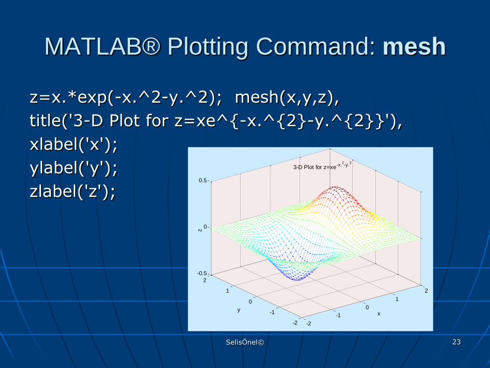
z=x.*exp(-x.^2-y.^2); mesh(x,y,z),
title('3-D Plot for z=xe^{-x.^{2}-y.^{2}}'),
xlabel('x');
ylabel('y');
zlabel('z');
-2
-1
0
1
2
-2
-1
0
1
2
-0.5
0
0.5
x
3-D Plot for z=xe-x.2-y.
2
y
z
SelisÖnel© 24
2.5-D Graphs: Surface
Used for visualizing a 3-D graph on a 2-D system of coordinates, i.e.,
showing different z-levels on an x-y system of coordinates by its contour lines
Ex: contour(x,y,z)
SelisÖnel© 25
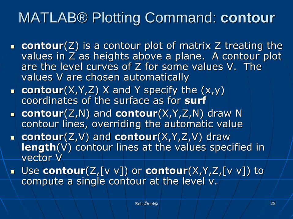
MATLAB® Plotting Command: contour
contour(Z) is a contour plot of matrix Z treating the values in Z as heights above a plane. A contour plot are the level curves of Z for some values V. The values V are chosen automatically
contour(X,Y,Z) X and Y specify the (x,y) coordinates of the surface as for surf
contour(Z,N) and contour(X,Y,Z,N) draw N contour lines, overriding the automatic value
contour(Z,V) and contour(X,Y,Z,V) draw length(V) contour lines at the values specified in vector V
Use contour(Z,[v v]) or contour(X,Y,Z,[v v]) to compute a single contour at the level v.
SelisÖnel© 26
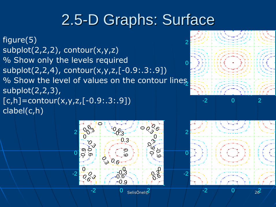
2.5-D Graphs: Surface figure(5)
subplot(2,2,2), contour(x,y,z)
% Show only the levels required
subplot(2,2,4), contour(x,y,z,[-0.9:.3:.9])
% Show the level of values on the contour lines
subplot(2,2,3),
[c,h]=contour(x,y,z,[-0.9:.3:.9])
clabel(c,h)
-2 0 2
-2
0
2
-2 0 2
-2
0
2
-0.9
-0.9
-0.9
-0.6
-0.6
-0.6
-0.6
-0.3
-0.3
-0.3 -0.3
0 0
0
0
0
0
0
0.3
0.3
0.3
0.3
0.3
0.3
0.6
0.6
0.6
0.6
0.6
0.9
-2 0 2
-2
0
2
SelisÖnel© 27
Other Plot Commands waterfall(...): Same as mesh(...) except that the
column lines of the mesh are not drawn - thus producing a "waterfall" plot. For column-oriented data analysis, use waterfall(z') or waterfall(x',y',z')
ribbon: Draws 2-D lines as ribbons in 3-D
ribbon(x,y) is the same as plot(x,y) except that the columns of
y are plotted as separated ribbons in 3-D. ribbon(y) uses the
default value of x=1:size(y,1).
ribbon(x,y,width) specifies the width of the ribbons to be width. The default value is width = 0.75;

SelisÖnel© 28
Other Plot Commands
spy : Zero/nonzero values, i.e., it visualizes sparsity pattern.
spy(S) plots the sparsity pattern of the matrix S
spy(S,'LineSpec') uses the color and marker from the line
specification string 'LineSpec'
surfl : 3-D shaded surface plot with light effects
same as surf(...) except that it draws the surface with highlights from a light source
SelisÖnel© 29
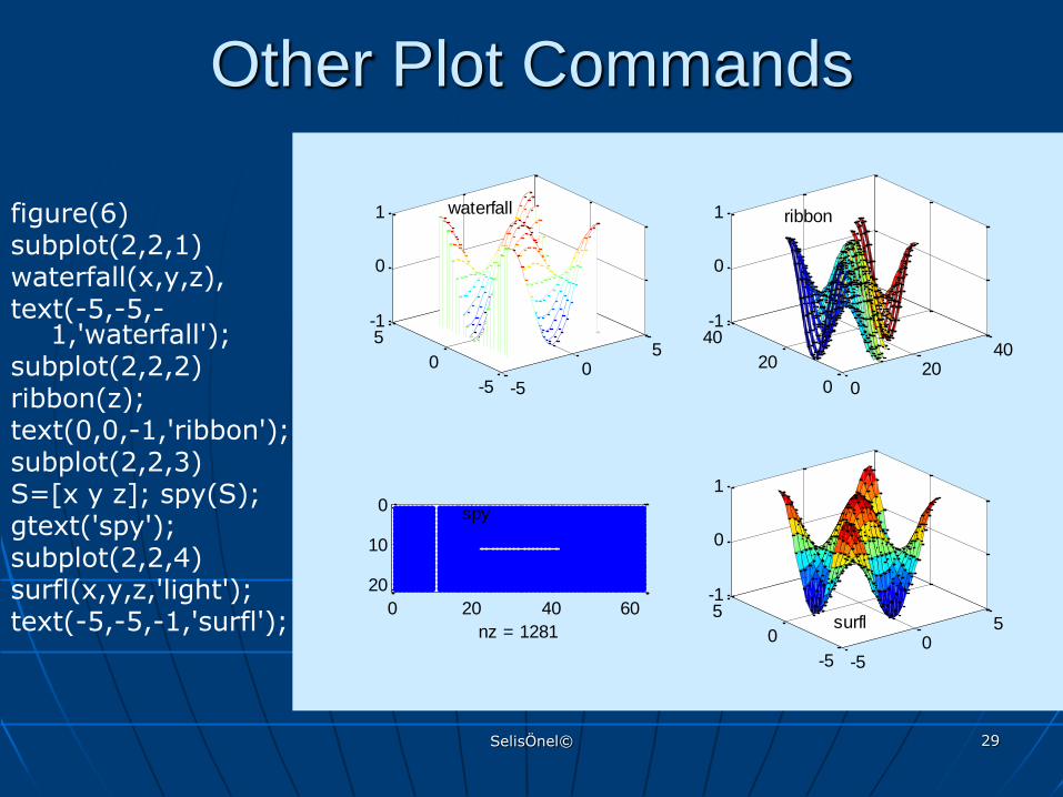
Other Plot Commands
figure(6) subplot(2,2,1) waterfall(x,y,z), text(-5,-5,-
1,'waterfall'); subplot(2,2,2) ribbon(z); text(0,0,-1,'ribbon'); subplot(2,2,3) S=[x y z]; spy(S); gtext('spy'); subplot(2,2,4) surfl(x,y,z,'light'); text(-5,-5,-1,'surfl');
-50
5
-5
0
5-1
0
1 waterfall
020
40
0
20
40-1
0
1 ribbon
0 20 40 60
0
10
20
nz = 1281
spy
-50
5
-5
0
5-1
0
1
surfl

SelisÖnel© 30
Data Export and Import
A=magic(3); B=magic(4); % save all variables in MATLAB® workspace save f1 % to save only certain variables save f2 A %These files have .mat extension and can only be
retrieved by MATLAB® % to load use: load f1 % To save data as text save f3 B –ascii
SelisÖnel© 31
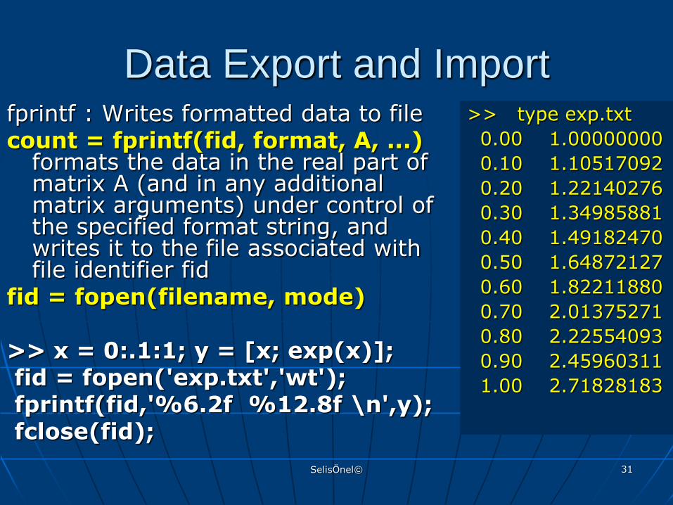
Data Export and Import fprintf : Writes formatted data to file count = fprintf(fid, format, A, ...)
formats the data in the real part of matrix A (and in any additional matrix arguments) under control of the specified format string, and writes it to the file associated with file identifier fid
fid = fopen(filename, mode) >> x = 0:.1:1; y = [x; exp(x)]; fid = fopen('exp.txt','wt'); fprintf(fid,'%6.2f %12.8f \n',y); fclose(fid);
>> type exp.txt
0.00 1.00000000
0.10 1.10517092
0.20 1.22140276
0.30 1.34985881
0.40 1.49182470
0.50 1.64872127
0.60 1.82211880
0.70 2.01375271
0.80 2.22554093
0.90 2.45960311
1.00 2.71828183
SelisÖnel© 32
Data Export and Import fread : Reads binary data from file. A = fread(FID) reads binary data from the
specified file and writes it into matrix A. FID is an integer file identifier obtained from fopen.
A = fread(FID,SIZE,PRECISION) reads the file
according to the data format specified by the string PRECISION. Valid entries for SIZE are:
N read N elements into a column vector. inf read to the end of the file. [M,N] read elements to fill an M-by-N matrix,
in column order. N can be inf, but M can't.
SelisÖnel© 33
Successive Substitution Iteration
Nonlinear system of equations usually can be written in the same form as linear equations Ax=y
Then, the coefficient matrix A and the inhomogeneous term y may be dependent on the solution
So, an iterative solution for a nonlinear system can be written as:
An-1xn=yn-1

SelisÖnel© 34
Successive Substitution Iteration
An-1xn=yn-1 can be solved using successive substitution iteration, where
An-1 : is computed using the most recent calculation result for xn
xn : is the nth iterative solution
yn-1 : is an inhomogeneous term assumed to be a function of xn

SelisÖnel© 35
Successive Substitution Iteration
1. Start the iteration with an initial guess for the solution x
2. Determine the coefficient matrix
3. Solve the system as a linear system
4. Get the solution x
5. Rearrange the coefficient matrix
6. Solve the system again
7. In case of instability:
8. Add the (under)relaxation parameter, i.e.
xn=ωinv(An-1)yn-1+(1-ω)xn-1 where 0<ω<1

SelisÖnel© 36
Electric circuit between heating elements can be shown schematically as: The resistance of the jth heating element is a function of temperature:
Rj=aj+bjTj+cjTj2 ,where
aj, bj, cj : constants Tj :temperature of the jth element Temperature of each heating element is determined by:
Ij2Rj=Ajσ(Tj
4-T∞4)+Ajh(Tj-T∞) , where
T∞ : temperature of the surrounding environment
Aj : the surface area of the jth element
Ex: Successive Substitution Iteration
I1 I2
R1 R2
R3 R4 100 V
SelisÖnel© 37
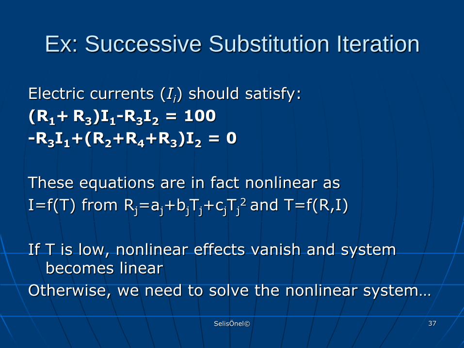
Ex: Successive Substitution Iteration
Electric currents (Ii) should satisfy:
(R1+ R3)I1-R3I2 = 100
-R3I1+(R2+R4+R3)I2 = 0
These equations are in fact nonlinear as
I=f(T) from Rj=aj+bjTj+cjTj2 and T=f(R,I)
If T is low, nonlinear effects vanish and system becomes linear
Otherwise, we need to solve the nonlinear system…
SelisÖnel© 38
Ex: Successive Substitution Iteration
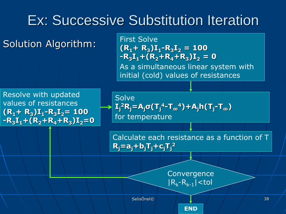
Solution Algorithm:
First Solve (R1+ R3)I1-R3I2 = 100 -R3I1+(R2+R4+R3)I2 = 0
As a simultaneous linear system with initial (cold) values of resistances
Solve Ij
2Rj=Ajσ(Tj4-T∞
4)+Ajh(Tj-T∞)
for temperature
Calculate each resistance as a function of T Rj=aj+bjTj+cjTj
2
Convergence |Rk-Rk-1|<tol
Resolve with updated values of resistances (R1+ R3)I1-R3I2= 100 -R3I1+(R2+R4+R3)I2=0
END

SelisÖnel© 39
Quiz
Find the roots of the following nonlinear system of equations using substitutive iteration.
Start with initial guess values of [3/4 2/3]
Show three consecutive iterations and check convergence for a tolerance of 0.0001
f(x,y)=x2+y2-1
g(x,y)=x2-y

SelisÖnel© 40
2.5-D Graph in MATLAB®
>> x1=-2:0.01:2;
>> x2=-2:0.01:2;
>> [x,y]=meshgrid(x1,x2);
>> f1=x.^2+y.^2-1 ;
>> f2=x.^2-y;
>> [c,h] = contour(f1); clabel(c,h),
colormap hsv, hold on,
>> [c,h] = contour(f2); clabel(c,h),
colorbar, hold off
0
0
0
0
0
1
11
1
11
1
22
2
2
2
22
2
33
3
3
3
3
3
3
34
4
4
4
5
5
5
5
6
6
6
6
-1
-10
0
0
01
11
1
1
2
2
2
2
2
2
3
3
3
3
4
4
4
4
5
5
50 100 150 200 250 300 350 400
50
100
150
200
250
300
350
400
-2
-1
0
1
2
3
4
5
6
SelisÖnel© 41
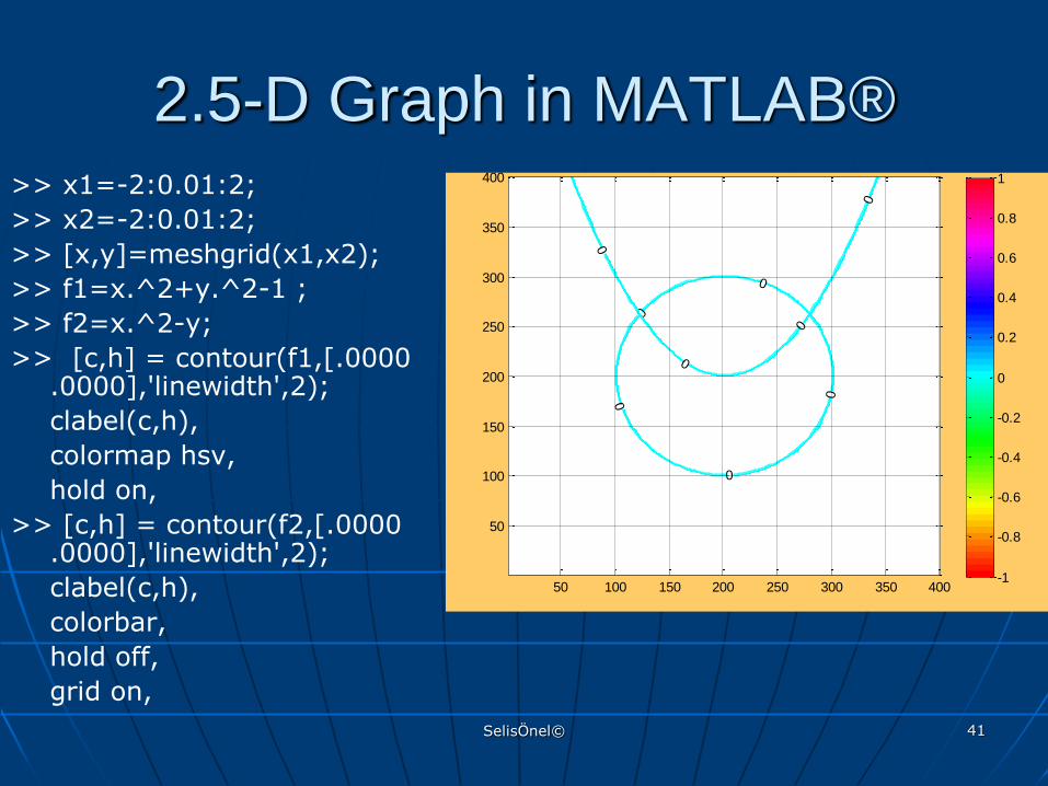
2.5-D Graph in MATLAB® >> x1=-2:0.01:2;
>> x2=-2:0.01:2;
>> [x,y]=meshgrid(x1,x2);
>> f1=x.^2+y.^2-1 ;
>> f2=x.^2-y;
>> [c,h] = contour(f1,[.0000 .0000],'linewidth',2);
clabel(c,h),
colormap hsv,
hold on,
>> [c,h] = contour(f2,[.0000 .0000],'linewidth',2);
clabel(c,h),
colorbar,
hold off,
grid on,
0
0
0
0
0
0
0
0
0
50 100 150 200 250 300 350 400
50
100
150
200
250
300
350
400
-1
-0.8
-0.6
-0.4
-0.2
0
0.2
0.4
0.6
0.8
1

SelisÖnel© 42
Ex: Plotting two functions in MATLAB® clear, clf, hold off x1=0:0.1:2; y1=-2:0.1:2; [x,y]=meshgrid(x1,y1); [f1,f2]=funnonlin(x,y); figure(1) subplot(1,2,1) mesh(f1,'linewidth',2), hold on, mesh(f2,'linewidth',2), axis([min(x1) max(x1) min(y1) max(y1) -10 10]); xlabel('x'); ylabel('y'); zlabel('z'); grid on; hold off, subplot(1,2,2) [c,h]=contour(x,y,f1,'-r','linewidth',2); clabel(c,h); hold on [c,h]=contour(x,y,f2,'linewidth',2); clabel(c,h); hold off axis([min(x1) max(x1) min(y1) max(y1)]); xlabel('x'); ylabel('y'); grid on; legend('f1','f2‘,2) x2=0:0.1:20; y2=-2:0.1:20; [x,y]=meshgrid(x2,y2); [f1,f2]=funnonlin(x,y); figure(2) subplot(1,2,1) mesh(f1), hold on, mesh(f2), axis([min(x2) max(x2) min(y2) max(y2) -10 10]); xlabel('x'); ylabel('y'); zlabel('z'); grid on; hold off, subplot(1,2,2) [c,h]=contour(x,y,f1,'-r','linewidth',2); clabel(c,h); hold on [c,h]=contour(x,y,f2,'linewidth',2); clabel(c,h); hold off axis([min(x1) max(x1) min(y1) max(y1)]); xlabel('x'); ylabel('y'); grid on; legend('f1','f2')

SelisÖnel© 43
Plotting two functions in MATLAB®
0
1
2
-2
0
2
-10
-5
0
5
10
xy
z
0
0
00
50
50
50 50
100
150-15-10
-5
0
0
0
x
y
0 0.5 1 1.5 2-2
-1.5
-1
-0.5
0
0.5
1
1.5
2
f1
f2
0
10
20
0
10
20
-10
-5
0
5
10
xy
z
0 00 0
00
x
y
0 5 10 15 20-2
0
2
4
6
8
10
12
14
16
18
20
f1
f2