sorbonne universite´, univ rennes and criteo ai labz · sorbonne universite´, univ rennesyand...
TRANSCRIPT

Submitted to the Annals of Statistics
SOME THEORETICAL PROPERTIES OF GANS
BY GERARD BIAU∗, BENOIT CADRE†, MAXIME SANGNIER∗ AND UGO
TANIELIAN∗,‡
Sorbonne Universite∗, Univ Rennes† and Criteo AI Lab‡
Generative Adversarial Networks (GANs) are a class of generative algo-rithms that have been shown to produce state-of-the-art samples, especially inthe domain of image creation. The fundamental principle of GANs is to ap-proximate the unknown distribution of a given data set by optimizing an ob-jective function through an adversarial game between a family of generatorsand a family of discriminators. In this paper, we offer a better theoretical un-derstanding of GANs by analyzing some of their mathematical and statisticalproperties. We study the deep connection between the adversarial principleunderlying GANs and the Jensen-Shannon divergence, together with someoptimality characteristics of the problem. An analysis of the role of the dis-criminator family via approximation arguments is also provided. In addition,taking a statistical point of view, we study the large sample properties of theestimated distribution and prove in particular a central limit theorem. Someof our results are illustrated with simulated examples.
1. Introduction. The fields of machine learning and artificial intelligence ha-ve seen spectacular advances in recent years, one of the most promising beingperhaps the success of Generative Adversarial Networks (GANs), introduced byGoodfellow et al. (2014). GANs are a class of generative algorithms implementedby a system of two neural networks contesting with each other in a zero-sum gameframework. This technique is now recognized as being capable of generating pho-tographs that look authentic to human observers (e.g., Salimans et al., 2016), andits spectrum of applications is growing at a fast pace, with impressive results in thedomains of inpainting, speech, and 3D modeling, to name but a few. A survey ofthe most recent advances is given by Goodfellow (2016).
The objective of GANs is to generate fake observations of a target distributionp? from which only a true sample (e.g., real-life images represented using raw pix-els) is available. It should be pointed out at the outset that the data involved in thedomain are usually so complex that no exhaustive description of p? by a classi-cal parametric model is appropriate, nor its estimation by a traditional maximumlikelihood approach. Similarly, the dimension of the samples is often very large,and this effectively excludes a strategy based on nonparametric density estimation
MSC 2010 subject classifications: Primary 62F12; secondary 68T01Keywords and phrases: generative models, adversarial principle, Jensen-Shannon divergence,
neural networks, central limit theorem
1imsart-aos ver. 2014/10/16 file: bcst.tex date: May 3, 2019

2 G. BIAU ET AL.
techniques such as kernel or nearest neighbor smoothing, for example. In order togenerate according to p?, GANs proceed by an adversarial scheme involving twocomponents: a family of generators and a family of discriminators, which are bothimplemented by neural networks. The generators admit low-dimensional randomobservations with a known distribution (typically Gaussian or uniform) as input,and attempt to transform them into fake data that can match the distribution p?;on the other hand, the discriminators aim to accurately discriminate between thetrue observations from p? and those produced by the generators. The generatorsand the discriminators are calibrated by optimizing an objective function in such away that the distribution of the generated sample is as indistinguishable as possiblefrom that of the original data. In pictorial terms, this process is often compared to agame of cops and robbers, in which a team of counterfeiters illegally produces ban-knotes and tries to make them undetectable in the eyes of a team of police officers,whose objective is of course the opposite. The competition pushes both teams toimprove their methods until counterfeit money becomes indistinguishable (or not)from genuine currency.
From a mathematical point of view, here is how the generative process of GANscan be represented. All the densities that we consider in the article are supposed tobe dominated by a fixed, known, measure µ on E, where E is a Borel subset ofRd .Depending on the practical context, this dominating measure may be the Lebesguemeasure, the counting measure, or more generally the Hausdorff measure on somesubmanifold of Rd . We assume to have at hand an i.i.d. sample X1, . . . ,Xn, drawnaccording to some unknown density p? on E. These random variables model theavailable data, such as images or video sequences; they typically take their valuesin a high-dimensional space, so that the ambient dimension d must be thought ofas large. The generators as a whole have the form of a parametric family of func-tions from Rd′ to E (usually, d′� d), say G = {Gθ}θ∈Θ , Θ ⊂Rp. Each functionGθ is intended to be applied to a d′-dimensional random variable Z (sometimescalled the noise—in most cases Gaussian or uniform), so that there is a naturalfamily of densities associated with the generators, say P = {pθ}θ∈Θ , where, by
definition, Gθ (Z)L= pθ dµ . In this model, each density pθ is a potential candidate
to represent p?. On the other hand, the discriminators are described by a family ofBorel functions from E to [0,1], say D , where each D ∈ D must be thought of asthe probability that an observation comes from p? (the higher D(x), the higher theprobability that x is drawn from p?). At some point, but not always, we will assumethat D is in fact a parametric class, of the form {Dα}α∈Λ , Λ ⊂ Rq, as is alwaysthe case in practice. In GANs algorithms, both parametric models {Gθ}θ∈Θ and{Dα}α∈Λ take the form of neural networks, but this does not play a fundamentalrole in this paper. We will simply remember that the dimensions p and q are poten-tially very large, which takes us away from a classical parametric setting. We also
imsart-aos ver. 2014/10/16 file: bcst.tex date: May 3, 2019

SOME THEORETICAL PROPERTIES OF GANS 3
insist on the fact that it is not assumed that p? belongs to P .Let Z1, . . . ,Zn be an i.i.d. sample of random variables, all distributed as the noise
Z. The objective is to solve in θ the problem
(1.1) infθ∈Θ
supD∈D
[ n
∏i=1
D(Xi)×n
∏i=1
(1−D◦Gθ (Zi))],
or, equivalently, to find θ ∈Θ such that
(1.2) supD∈D
L(θ ,D)≤ supD∈D
L(θ ,D), ∀θ ∈Θ ,
where
L(θ ,D)def=
1n
n
∑i=1
lnD(Xi)+1n
n
∑i=1
ln(1−D◦Gθ (Zi))
(ln is the natural logarithm). The zero-sum game (1.1) is the statistical translationof making the distribution of Gθ (Zi) (i.e., pθ ) as indistinguishable as possible fromthat of Xi (i.e., p?). Here, distinguishability is understood as the capability to deter-mine from which distribution an observation x comes from. Mathematically, thisis captured by the discrimination value D(x), which represents the probability thatx comes from p? rather than from pθ . Therefore, for a given θ , the discrimina-tor D is determined so as to be maximal on the Xi and minimal on the Gθ (Zi). Inthe most favorable situation (that is, when the two samples are scattered by D),supD∈D L(θ ,D) is zero, and the larger this quantity, the more distinguishable thetwo samples are. Hence, in order to make the distribution pθ as indistinguishableas possible from p?, Gθ has to be driven so as to minimize supD∈D L(θ ,D).
As mentioned above, this adversarial problem is often illustrated by the strug-gle between a police team (the discriminators), trying to distinguish true banknotesfrom false ones (respectively, the Xi and the Gθ (Zi)), and a counterfeiters team,slaving to produce banknotes as credible as possible and to mislead the police.Obviously, their objectives (represented by the quantity L(θ ,D)) are exactly op-posite. All in all, we see that the criterion seeks to find the right balance be-tween the conflicting interests of the generators and the discriminators. The hopeis that the θ achieving equilibrium will make it possible to generate observationsG
θ(Z1), . . . ,Gθ
(Zn) indistinguishable from reality, i.e., observations with a distri-bution close to the unknown p?.
The criterion L(θ ,D) involved in (1.2) is the criterion originally proposed inthe adversarial framework of Goodfellow et al. (2014). Since then, the success ofGANs in applications has led to a large volume of literature on variants, which allhave many desirable properties but are based on different optimization criteria: ex-amples are MMD-GANs (Dziugaite et al., 2015), f-GANs (Nowozin et al., 2016),Wasserstein-GANs (Arjovsky et al., 2017), and an approach based on scattering
imsart-aos ver. 2014/10/16 file: bcst.tex date: May 3, 2019

4 G. BIAU ET AL.
transforms (Angles and Mallat, 2018). All these variations and their innumerablealgorithmic versions constitute the galaxy of GANs. That being said, despite in-creasingly spectacular applications, little is known about the mathematical and sta-tistical forces behind these algorithms (e.g., Arjovsky and Bottou, 2017; Liu et al.,2017; Liang, 2018; Zhang et al., 2018), and, in fact, nearly nothing about the pri-mary adversarial problem (1.2). As acknowledged by Liu et al. (2017), basic ques-tions on how well GANs can approximate the target distribution p? remain largelyunanswered. In particular, the role and impact of the discriminators on the qual-ity of the approximation are still a mystery, and simple but fundamental questionsregarding statistical consistency and rates of convergence remain open.
In the present article, we propose to take a small step towards a better theoreti-cal understanding of GANs by analyzing some of the mathematical and statisticalproperties of the original adversarial problem (1.2). In Section 2, we study thedeep connection between the population version of (1.2) and the Jensen-Shannondivergence, together with some optimality characteristics of the problem, often re-ferred to in the literature but in fact poorly understood. Section 3 is devoted to abetter comprehension of the role of the discriminator family via approximation ar-guments. Finally, taking a statistical point of view, we study in Section 4 the largesample properties of the distribution p
θand of θ , and prove in particular a central
limit theorem for this parameter. Section 5 summarizes the main results and dis-cusses research directions for future work. For clarity, most technical proofs aregathered in Section 6. Some of our results are illustrated with simulated examples.
2. Optimality properties. We start by studying some important properties ofthe adversarial principle, emphasizing the role played by the Jensen-Shannon diver-gence. We recall that if P and Q are probability measures on E, and P is absolutelycontinuous with respect to Q, then the Kullback-Leibler divergence from Q to P isdefined as
DKL(P ‖ Q) =∫
lndPdQ
dP,
where dPdQ is the Radon-Nikodym derivative of P with respect to Q. The Kullback-
Leibler divergence is always nonnegative, with DKL(P ‖ Q) zero if and only ifP = Q. If p = dP
dµand q = dQ
dµexist (meaning that P and Q are absolutely continuous
with respect to µ , with densities p and q), then the Kullback-Leibler divergence isgiven as
DKL(P ‖ Q) =∫
p lnpq
dµ,
and alternatively denoted by DKL(p ‖ q). We also recall that the Jensen-Shannondivergence is a symmetrized version of the Kullback-Leibler divergence. It is de-
imsart-aos ver. 2014/10/16 file: bcst.tex date: May 3, 2019

SOME THEORETICAL PROPERTIES OF GANS 5
fined for any probability measures P and Q on E by
DJS(P,Q) =12
DKL
(P∥∥∥ P+Q
2
)+
12
DKL
(Q∥∥∥ P+Q
2
),
and satisfies 0 ≤ DJS(P,Q) ≤ ln2. The square root of the Jensen-Shannon diver-gence is a metric often referred to as Jensen-Shannon distance (Endres and Schin-delin, 2003). When P and Q have densities p and q with respect to µ , we use thenotation DJS(p,q) in place of DJS(P,Q).
For a generator Gθ and an arbitrary discriminator D ∈ D , the criterion L(θ ,D)to be optimized in (1.2) is but the empirical version of the probabilistic criterion
L(θ ,D)def=∫
ln(D)p?dµ +∫
ln(1−D)pθ dµ.
We assume for the moment that the discriminator class D is not restricted andequals D∞, the set of all Borel functions from E to [0,1]. We note however that, forall θ ∈Θ ,
0≥ supD∈D∞
L(θ ,D)≥− ln2(∫
p?dµ +∫
pθ dµ
)=− ln4,
so that infθ∈Θ supD∈D∞L(θ ,D) ∈ [− ln4,0]. Thus,
infθ∈Θ
supD∈D∞
L(θ ,D) = infθ∈Θ
supD∈D∞:L(θ ,D)>−∞
L(θ ,D).
This identity points out the importance of discriminators such that L(θ ,D)>−∞,which we call θ -admissible. In the sequel, in order to avoid unnecessary problemsof integrability, we only consider such discriminators, keeping in mind that theothers have no interest.
Of course, working with D∞ is somehow an idealized vision, since in practicethe discriminators are always parameterized by some parameter α ∈ Λ , Λ ⊂ Rq.Nevertheless, this point of view is informative and, in fact, is at the core of theconnection between our generative problem and the Jensen-Shannon divergence.Indeed, taking the supremum of L(θ ,D) over D∞, we have
supD∈D∞
L(θ ,D) = supD∈D∞
∫ [ln(D)p?+ ln(1−D)pθ
]dµ
≤∫
supD∈D∞
[ln(D)p?+ ln(1−D)pθ
]dµ
= L(θ ,D?θ ),
where
(2.1) D?θ
def=
p?
p?+ pθ
.
imsart-aos ver. 2014/10/16 file: bcst.tex date: May 3, 2019

6 G. BIAU ET AL.
(We use throughout the convention 0/0 = 0 and ∞× 0 = 0.) By observing thatL(θ ,D?
θ) = 2DJS(p?, pθ )− ln4, we conclude that, for all θ ∈Θ ,
supD∈D∞
L(θ ,D) = L(θ ,D?θ ) = 2DJS(p?, pθ )− ln4.
We note in particular that D?θ
is θ -admissible. The fact that D?θ
realizes the supre-mum of L(θ ,D) over D∞ and that this supremum is connected to the Jensen-Shannon divergence between p? and pθ appears in the original article by Goodfel-low et al. (2014). This remark has given rise to many developments that interpretthe adversarial problem (1.2) as the empirical version of the minimization probleminfθ DJS(p?, pθ ) over Θ . Accordingly, many GANs algorithms try to learn the op-timal function D?
θ, using for example stochastic gradient descent techniques and
mini-batch approaches. However, it remains to prove that D?θ
is unique as a max-imizer of L(θ ,D) over all D. The following theorem, which completes a result of(Goodfellow et al., 2014), shows that this is the case in some situations.
THEOREM 2.1. Let θ ∈Θ and D ∈D∞ be such that L(θ ,D) = L(θ ,D?θ). Then
D = D?θ
µ-almost everywhere on the complementary of the set {p? = pθ = 0}. Inparticular, if µ({p? = pθ = 0}) = 0, then the function D?
θis the unique discrimi-
nator that achieves the supremum of the functional D 7→ L(θ ,D) over D∞, i.e.,
{D?θ}=argmax
D∈D∞
L(θ ,D).
Before proving the theorem, it is important to note that if we dot not assumethat µ({p? = pθ = 0}) = 0, then we cannot conclude that D = D?
θµ-almost every-
where. To see this, suppose that pθ = p?. Then, whatever D ∈D∞ is, the discrimi-nator D?
θ1{pθ>0}+ D1{pθ=0} satisfies
L(θ ,D?θ 1{pθ>0}+ D1{pθ=0}) = L(θ ,D?
θ ).
This simple counterexample shows that uniqueness of the optimal discriminatordoes not hold in general.
PROOF. Let D∈D∞ be a discriminator such that L(θ ,D) = L(θ ,D?θ). In partic-
ular, L(θ ,D) > −∞ and D is θ -admissible. Thus, letting A def= {p? = pθ = 0} and
fα
def= p? ln(α)+ pθ ln(1−α) for α ∈ [0,1], we see that∫
Ac( fD− fD?
θ)dµ = 0.
Since, on Ac,fD ≤ sup
α∈[0,1]fα = fD?
θ,
imsart-aos ver. 2014/10/16 file: bcst.tex date: May 3, 2019

SOME THEORETICAL PROPERTIES OF GANS 7
we have fD = fD?θ
µ-almost everywhere on Ac. By uniqueness of the maximizer ofα 7→ fα on Ac, we conclude that D = D?
θµ-almost everywhere on Ac.
By definition of the optimal discriminator D?θ
, we have
L(θ ,D?θ ) = sup
D∈D∞
L(θ ,D) = 2DJS(p?, pθ )− ln4, ∀θ ∈Θ .
Therefore, it makes sense to let the parameter θ ? ∈Θ be defined as
L(θ ?,D?θ ?)≤ L(θ ,D?
θ ), ∀θ ∈Θ ,
or, equivalently,
(2.2) DJS(p?, pθ ?)≤ DJS(p?, pθ ), ∀θ ∈Θ .
The parameter θ ? may be interpreted as the best parameter in Θ for approaching theunknown density p? in terms of Jensen-Shannon divergence, in a context where allpossible discriminators are available. In other words, the generator Gθ ? is the idealgenerator, and the density pθ ? is the one we would ideally like to use to generatefake samples. Of course, whenever p? ∈P (i.e., the target density is in the model),then p? = pθ ? , DJS(p?, pθ ?) = 0, and D?
θ ? = 1/2. This is, however, a very specialcase, which is of no interest, since in the applications covered by GANs, the dataare usually so complex that the hypothesis p? ∈P does not hold.
In the general case, our next theorem provides sufficient conditions for the ex-istence and uniqueness of θ ?. For P and Q probability measures on E, we letδ (P,Q) =
√DJS(P,Q), and recall that δ is a distance on the set of probability mea-
sures on E (Endres and Schindelin, 2003). We let dP? = p?dµ and, for all θ ∈Θ ,dPθ = pθ dµ .
THEOREM 2.2. Assume that the model P = {Pθ}θ∈Θ is convex and compactfor the metric δ . If p? > 0 µ-almost everywhere, then there exists a unique p ∈Psuch that
{ p}=argminp∈P
DJS(p?, p).
In particular, if the model P is identifiable, then
{θ ?}=argminθ∈Θ
L(θ ,D?θ )
or, equivalently,{θ ?}=argmin
θ∈Θ
DJS(p?, pθ ).
imsart-aos ver. 2014/10/16 file: bcst.tex date: May 3, 2019

8 G. BIAU ET AL.
We note that the identifiability assumption in the second statement of the theo-rem is hardly satisfied in the high-dimensional context of (deep) neural networks.In this case, it is likely that several parameters θ yield the same function (genera-tor), so that the parametric setting is potentially misspecified. However, if we thinkin terms of distributions instead of parameters, then the first part of Theorem 2.2ensures existence and uniqueness of the optimum.
PROOF. Assuming the first part of the theorem, the second one is obvious sinceL(θ ,D?
θ)= supD∈D∞
L(θ ,D) = 2DJS(p?, pθ )− ln4. Therefore, it is enough to provethat there exists a unique density p of P such that
{ p}=argminp∈P
DJS(p?, p).
Existence. Since P is compact for δ , it is enough to show that the function
P → R+
P 7→ DJS(P?,P)
is continuous. But this is clear since, for all P1,P2 ∈P , |δ (P?,P1)− δ (P?,P2)| ≤δ (P1,P2) by the triangle inequality. Therefore, argminp∈PDJS(p?, p) 6= /0.
Uniqueness. For a≥ 0, we consider the function Fa defined by
Fa(x) = a ln( 2a
a+ x
)+ x ln
( 2xa+ x
), x≥ 0,
with the convention 0ln0 = 0. Clearly, F ′′a (x) =a
x(a+x) , which shows that Fa isstrictly convex whenever a > 0. We now proceed to prove that L1(µ)⊃P 3 p 7→DJS(p?, p) is strictly convex as well. Let λ ∈ (0,1) and p1, p2 ∈P with p1 6= p2,i.e., µ({p1 6= p2})> 0. Then
DJS(p?,λ p1 +(1−λ )p2)
=∫
Fp?(λ p1 +(1−λ )p2)dµ
=∫{p1=p2}
Fp?(p1)dµ +∫{p1 6=p2}
Fp?(λ p1 +(1−λ )p2)dµ.
By the strict convexity of Fp? over {p? > 0}, we obtain
DJS(p?,λ p1 +(1−λ )p2)
<∫{p1=p2}
Fp?(p1)dµ +λ
∫{p1 6=p2}
Fp?(p1)dµ +(1−λ )∫{p1 6=p2}
Fp?(p2)dµ,
imsart-aos ver. 2014/10/16 file: bcst.tex date: May 3, 2019

SOME THEORETICAL PROPERTIES OF GANS 9
which implies
DJS(p?,λ p1 +(1−λ )p2)< λDJS(p?, p1)+(1−λ )DJS(p?, p2).
Consequently, the function L1(µ)⊃P 3 p 7→DJS(p?, p) is strictly convex, and itsargmin over the convex set P is either the empty set or a singleton.
REMARK 2.1. There are simple conditions for the model P = {Pθ}θ∈Θ to becompact for the metric δ . It is for example enough to suppose that Θ is compact,P is convex, and
(i) For all x ∈ E, the function θ 7→ pθ (x) is continuous on Θ ;(ii) One has sup(θ ,θ ′)∈Θ 2 |pθ ln pθ ′ | ∈ L1(µ).
Let us quickly check that under these conditions, P is compact for the metric δ .Since Θ is compact, by the sequential characterization of compact sets, it is enoughto prove that if Θ ⊃ (θn)n converges to θ ∈Θ , then DJS(pθ , pθn)→ 0. But,
DJS(pθ , pθn) =∫ [
pθ ln( 2pθ
pθ + pθn
)+ pθn ln
( 2pθn
pθ + pθn
)]dµ.
By the convexity of P , using (i) and (ii), the Lebesgue dominated convergencetheorem shows that DJS(pθ , pθn)→ 0, whence the result.
Interpreting the adversarial problem in connection with the optimization pro-gram infθ∈Θ DJS(p?, pθ ) is a bit misleading, because this is based on the assump-tion that all possible discriminators are available (and in particular the optimaldiscriminator D?
θ). In the end this means assuming that we know the distribution
p?, which is eventually not acceptable from a statistical perspective. In practice,the class of discriminators is always restricted to be a parametric family D ={Dα}α∈Λ , Λ ⊂ Rq, and it is with this class that we have to work. From our pointof view, problem (1.2) is a likelihood-type problem involving two parametric fam-ilies G and D , which must be analyzed as such, just as we would do for a classicalmaximum likelihood approach. In fact, it takes no more than a moment’s thoughtto realize that the key lies in the approximation capabilities of the discriminatorclass D with respect to the functions D?
θ, θ ∈Θ . This is the issue that we discuss
in the next section.
3. Approximation properties. In the remainder of the article, we assume thatθ ? exists, keeping in mind that Theorem 2.2 provides us with precise conditionsguaranteeing its existence and its uniqueness. As pointed out earlier, in practiceonly a parametric class D = {Dα}α∈Λ , Λ ⊂ Rq, is available, and it is thereforelogical to consider the parameter θ ∈Θ defined by
supD∈D
L(θ ,D)≤ supD∈D
L(θ ,D), ∀θ ∈Θ .
imsart-aos ver. 2014/10/16 file: bcst.tex date: May 3, 2019

10 G. BIAU ET AL.
(We assume for now that θ exists—sufficient conditions for this existence, relat-ing to compactness of Θ and regularity of the model P , will be given in the nextsection.) The density pθ is thus the best candidate to imitate pθ ? , given the para-metric families of generators G and discriminators D . The natural question is then:is it possible to quantify the proximity between pθ and the ideal pθ ? via the ap-proximation properties of the class D? In other words, if D is growing, is it truethat pθ approaches pθ ? , and in the affirmative, in which sense and at which speed?Theorem 3.1 below provides a first answer to this important question, in terms ofexcess of Jensen-Shannon error DJS(p?, pθ )−DJS(p?, pθ ?). To state the result, wewill need an assumption.
Let ‖ · ‖2 be the L2(µ) norm. Our condition guarantees that the parametric classD is rich enough to approach the discriminator D?
θin the L2 sense. In the remainder
of the section, it is assumed that D?θ∈ L2(µ).
Assumption (Hε) There exist ε > 0, m ∈ (0,1/2), and D ∈D ∩L2(µ) such thatm≤ D≤ 1−m and ‖D−D?
θ‖2 ≤ ε .
We observe in passing that such a discriminator D is θ -admissible. We are nowequipped to state our approximation theorem. For ease of reading, its proof is post-poned to Section 6.
THEOREM 3.1. Assume that, for some M > 0, p? ≤ M and pθ ≤ M. Then,under Assumption (Hε) with ε < 1/(2M), there exists a positive constant c (de-pending only upon m and M) such that
(3.1) 0≤ DJS(p?, pθ )−DJS(p?, pθ ?)≤ cε2.
This theorem points out that if the class D is rich enough to approximate thediscriminator D?
θin such a way that ‖D−D?
θ‖2 ≤ ε for some small ε , then working
with a restricted class of discriminators D instead of the set of all discriminatorsD∞ has an impact that is not larger than a O(ε2) factor with respect to the excess ofJensen-Shannon error. It shows in particular that the Jensen-Shannon divergence isa suitable criterion for the problem we are examining.
4. Statistical analysis. The data-dependent parameter θ , achieves the infi-mum of the adversarial problem (1.2). Practically speaking, it is this parameter thatwill be used in the end for producing fake data, via the associated generator G
θ.
We first study in Subsection 4.1 the large sample properties of the distribution pθ
via the excess of Jensen-Shannon error DJS(p?, pθ)−DJS(p?, pθ ?), and then state
in Subsection 4.2 the almost sure convergence and asymptotic normality of the pa-rameter θ as the sample size n tends to infinity. Throughout, the parameter sets Θ
and Λ are assumed to be compact subsets of Rp and Rq, respectively. To simplify
imsart-aos ver. 2014/10/16 file: bcst.tex date: May 3, 2019

SOME THEORETICAL PROPERTIES OF GANS 11
the analysis, we also assume that µ(E)< ∞. In this case, every discriminator is inLp(µ) for all p≥ 1.
4.1. Asymptotic properties of DJS(p?, pθ). As for now, we assume that we
have at hand a parametric family of generators G = {Gθ}θ∈Θ , Θ ⊂Rp, and a para-metric family of discriminators D = {Dα}α∈Λ , Λ ⊂Rq. We recall that the collec-
tion of probability densities associated with G is P = {pθ}θ∈Θ , where Gθ (Z)L=
pθ dµ and Z is some low-dimensional noise random variable. In order to avoid anyconfusion, for a given discriminator D = Dα we use the notation L(θ ,α) (respec-tively, L(θ ,α)) instead of L(θ ,D) (respectively, L(θ ,D)) when useful. So,
L(θ ,α) =1n
n
∑i=1
lnDα(Xi)+1n
n
∑i=1
ln(1−Dα ◦Gθ (Zi)),
andL(θ ,α) =
∫ln(Dα)p?dµ +
∫ln(1−Dα)pθ dµ.
We will need the following regularity assumptions:Assumptions (Hreg)
(HD) There exists κ ∈ (0,1/2) such that, for all α ∈Λ , κ ≤ Dα ≤ 1−κ . In addi-tion, the function (x,α) 7→ Dα(x) is of class C1, with a uniformly boundeddifferential.
(HG) For all z ∈ Rd′ , the function θ 7→ Gθ (z) is of class C1, uniformly bounded,with a uniformly bounded differential.
(Hp) For all x∈E, the function θ 7→ pθ (x) is of class C1, uniformly bounded, witha uniformly bounded differential.
Note that under (HD), all discriminators in {Dα}α∈Λ are θ -admissible, whateverθ . All of these requirements are classic regularity conditions for statistical models,which imply in particular that the functions L(θ ,α) and L(θ ,α) are continuous.Therefore, the compactness of Θ guarantees that θ and θ exist. Conditions for theexistence of θ ? are given in Theorem 2.2.
We have known since Theorem 3.1 that if the available class of discrimina-tors D approaches the optimal discriminator D?
θby a distance not more than ε ,
then DJS(p?, pθ )−DJS(p?, pθ ?) = O(ε2). It is therefore reasonable to expect that,asymptotically, the difference DJS(p?, p
θ)−DJS(p?, pθ ?) will not be larger than a
term proportional to ε2, in some probabilistic sense. This is precisely the result ofTheorem 4.1 below. In fact, most articles to date have focused on the developmentand analysis of optimization procedures (typically, stochastic-gradient-type algo-rithms) to compute θ , without really questioning its convergence properties as thedata set grows. Although our statistical results are theoretical in nature, we believe
imsart-aos ver. 2014/10/16 file: bcst.tex date: May 3, 2019

12 G. BIAU ET AL.
that they are complementary to the optimization literature, insofar as they offerguarantees on the validity of the algorithms.
In addition to the regularity hypotheses, we will need the following requirement,which is a stronger version of (Hε):
Assumption (H ′ε) There exist ε > 0 and m ∈ (0,1/2) such that: for all θ ∈Θ ,there exists D ∈D such that m≤ D≤ 1−m and ‖D−D?
θ‖2 ≤ ε .
We are ready to state our first statistical theorem.
THEOREM 4.1. Assume that, for some M > 0, p? ≤ M and pθ ≤ M for allθ ∈Θ . Then, under Assumptions (Hreg) and (H ′ε) with ε < 1/(2M), one has
EDJS(p?, pθ)−DJS(p?, pθ ?) = O
(ε
2 +1√n
).
REMARK 4.1. The constant hidden in the O term scales as p+ q. Knowingthat (deep) neural networks, and thus GANs, are often used in the so-called over-parameterized regime (i.e., when the number of parameters exceeds the number ofexamples), this limits the impact of the result in the neural network context, at leastwhen p+ q is large with respect to
√n. For instance, successful applications of
GANs on common datasets such as LSUN (√
n ≈ 1740) and FACES (√
n ≈ 590)make use of more than 1500000 parameters (Radford et al., 2016).
PROOF. Fix ε ∈ (0,1/(2M)) as in Assumption (H ′ε), and choose D ∈ D suchthat m≤ D≤ 1−m and ‖D−D?
θ‖2 ≤ ε . By repeating the arguments of the proof of
Theorem 3.1 (with θ instead of θ ), we conclude that there exists a constant c1 > 0such that
2DJS(p?, pθ)≤ c1ε
2 +L(θ , D)+ ln4≤ c1ε2 + sup
α∈Λ
L(θ ,α)+ ln4.
Therefore,
2DJS(p?, pθ)≤ c1ε
2 + supθ∈Θ ,α∈Λ
|L(θ ,α)−L(θ ,α)|+ supα∈Λ
L(θ ,α)+ ln4
= c1ε2 + sup
θ∈Θ ,α∈Λ
|L(θ ,α)−L(θ ,α)|+ infθ∈Θ
supα∈Λ
L(θ ,α)+ ln4
(by definition of θ )
≤ c1ε2 +2 sup
θ∈Θ ,α∈Λ
|L(θ ,α)−L(θ ,α)|+ infθ∈Θ
supα∈Λ
L(θ ,α)+ ln4.
imsart-aos ver. 2014/10/16 file: bcst.tex date: May 3, 2019

SOME THEORETICAL PROPERTIES OF GANS 13
So,
2DJS(p?, pθ)≤ c1ε
2 +2 supθ∈Θ ,α∈Λ
|L(θ ,α)−L(θ ,α)|+ infθ∈Θ
supD∈D∞
L(θ ,D)+ ln4
= c1ε2 +2 sup
θ∈Θ ,α∈Λ
|L(θ ,α)−L(θ ,α)|+L(θ ?,D?θ ?)+ ln4
(by definition of θ ?)
= c1ε2 +2DJS(p?, pθ ?)+2 sup
θ∈Θ ,α∈Λ
|L(θ ,α)−L(θ ,α)|.
Thus, letting c2 = c1/2, we have
(4.1) DJS(p?, pθ)−DJS(p?, pθ ?)≤ c2ε
2 + supθ∈Θ ,α∈Λ
|L(θ ,α)−L(θ ,α)|.
Clearly, under Assumptions (HD), (HG), and (Hp), (L(θ ,α)−L(θ ,α))θ∈Θ ,α∈Λ isa separable subgaussian process (e.g., van Handel, 2016, Chapter 5) for the distanced = S‖ · ‖/
√n, where ‖ · ‖ is the standard Euclidean norm on Rp×Rq and S > 0
depends only on the bounds in (HD) and (HG). Let N(Θ ×Λ ,‖ · ‖,u) denote theu-covering number of Θ ×Λ for the distance ‖ · ‖. Then, by Dudley’s inequality(van Handel, 2016, Corollary 5.25),
(4.2) E supθ∈Θ ,α∈Λ
|L(θ ,α)−L(θ ,α)| ≤ 12S√n
∫∞
0
√ln(N(Θ ×Λ ,‖ · ‖,u))du.
Since Θ and Λ are bounded, there exists r > 0 such that N(Θ ×Λ ,‖ · ‖,u) = 1 foru≥ r and
N(Θ ×Λ ,‖ · ‖,u) = O((√p+q
u
)p+q)for u < r.
Combining this inequality with (4.1) and (4.2), we obtain
EDJS(p?, pθ)−DJS(p?, pθ ?)≤ c3
(ε
2 +1√n
),
for some positive constant c3 that scales as p+ q. The conclusion follows by ob-serving that, by (2.2),
DJS(p?, pθ ?)≤ DJS(p?, pθ).
Theorem 4.1 is illustrated in Figure 1, which shows the approximate values ofEDJS(p?, p
θ). We took p?(x) = e−x/s
s(1+e−x/s)2 (centered logistic density with scale pa-rameter s = 0.33), and let G and D be two fully connected neural networks param-eterized by weights and offsets. The noise random variable Z follows a uniform
imsart-aos ver. 2014/10/16 file: bcst.tex date: May 3, 2019

14 G. BIAU ET AL.
distribution on [0,1], and the parameters of G and D are chosen in a sufficientlylarge compact set. In order to illustrate the impact of ε in Theorem 4.1, we fixedthe sample size to a large n = 100000 and varied the number of layers of the dis-criminators from 2 to 5, keeping in mind that a larger number of layers results ina smaller ε . To diversify the setting, we also varied the number of layers of thegenerators from 2 to 3. The expectation EDJS(p?, p
θ) was estimated by averaging
over 30 repetitions (the number of runs has been reduced for time complexity lim-itations). Note that we do not pay attention to the exact value of the constant termDJS(p?, pθ ?), which is intractable in our setting.
Fig 1: Bar plots of the Jensen-Shannon divergence DJS(p?, pθ) with respect to the
number of layers (depth) of both the discriminators and generators. The height ofeach rectangle estimates EDJS(p?, p
θ).
Figure 1 highlights thatEDJS(p?, pθ) approaches the value DJS(p?, pθ ?) as ε ↓ 0,
i.e., as the discriminator depth increases, given that the contribution of 1/√
n iscertainly negligible for n = 100000. Figure 2 shows the target density p? vs. thehistograms and kernel estimates of 100000 data sampled from G
θ(Z), in the two
cases: (discriminator depth = 2, generator depth = 3) and (discriminator depth = 5,generator depth = 3). In accordance with the decrease of EDJS(p?, p
θ), the estima-
tion of the true distribution p? improves when ε becomes small.
Some comments on the optimization scheme. Numerical optimization is quite atough point for GANs, partly due to nonconvex-concavity of the saddle point prob-lem described in equation (1.2) and the nondifferentiability of the objective func-tion. This motivates a very active line of research (e.g., Goodfellow et al., 2014;Nowozin et al., 2016; Arjovsky et al., 2017; Arjovsky and Bottou, 2017), which
imsart-aos ver. 2014/10/16 file: bcst.tex date: May 3, 2019

SOME THEORETICAL PROPERTIES OF GANS 15
(a) Discriminator depth = 2, generator depth = 3. (b) Discriminator depth = 5, generator depth = 3.
Fig 2: True density p?, histograms, and kernel estimates (continuous line) of100000 data sampled from G
θ(Z). Also shown is the final discriminator Dα .
aims at transforming the objective into a more convenient function and devisingefficient algorithms. In the present paper, since we are interested in original GANs,the algorithmic approach described by Goodfellow et al. (2014) is adopted, andnumerical optimization is performed thanks to the machine learning frameworkTensorFlow (Abadi et al., 2015), working with gradient descent based on auto-matic differentiation. As proposed by Goodfellow et al. (2014), the objective func-tion θ 7→ supα∈Λ L(θ ,α) is not directly minimized. We used instead an alternatedprocedure, which consists in iterating (a few hundred times in our examples) thefollowing two steps:
(i) For a fixed value of θ and from a given value of α , perform 10 ascent stepson L(θ , ·);
(ii) For a fixed value of α and from a given value of θ , perform 1 descent step onθ 7→ −∑
ni=1 ln(Dα ◦Gθ (Zi)) (instead of θ 7→ ∑
ni=1 ln(1−Dα ◦Gθ (Zi))).
This alternated procedure is motivated by two reasons. First, for a given θ , ap-proximating supα∈Λ L(θ ,α) is computationally prohibitive and may result in over-fitting the finite training sample (Goodfellow et al., 2014). This can be explainedby the shape of the function θ 7→ supα∈Λ L(θ ,α), which may be almost piecewiseconstant, resulting in a zero gradient almost everywhere (or at best very low; seeArjovsky et al., 2017). Next, empirically, − ln(Dα ◦Gθ (Zi)) provides bigger gra-dients than ln(1−Dα ◦Gθ (Zi)), resulting in a more powerful algorithm than theoriginal version, while leading to the same minimizers.
In all our experiments, the learning rates needed in gradient steps were fixed andtuned by hand, in order to prevent divergence. In addition, since our main objectiveis to focus on illustrating the statistical properties of GANs rather than delving intooptimization issues, we decided to perform mini-batch gradient updates instead ofstochastic ones (that is, new observations of X and Z are not sampled at each step
imsart-aos ver. 2014/10/16 file: bcst.tex date: May 3, 2019

16 G. BIAU ET AL.
of the procedure). This is different from what is done in the original algorithm ofGoodfellow et al. (2014).
All in all, we realize that our numerical approach—although widely adopted bythe machine learning community—may fail to locate the desired estimator θ (i.e.,the exact minimizer in θ of supα∈Λ L(θ ,α)) in more complex contexts than thosepresented in the present paper. It is nevertheless sufficient for our objective, whichis limited to illustrating the theoretical results with a few simple examples.
4.2. Asymptotic properties of θ . Theorem 4.1 states a result relative to theexcess of Jensen-Shannon error DJS(p?, p
θ)−DJS(p?, pθ ?). We now examine the
convergence properties of the parameter θ itself as the sample size n grows. Wewould typically like to find reasonable conditions ensuring that θ → θ almostsurely as n→ ∞. To reach this goal, we first need to strengthen a bit the Assump-tions (Hreg), as follows:
Assumptions (H ′reg)
(H ′D) There exists κ ∈ (0,1/2) such that, for all α ∈Λ , κ ≤ Dα ≤ 1−κ . In addi-tion, the function (x,α) 7→ Dα(x) is of class C2, with differentials of order 1and 2 uniformly bounded.
(H ′G) For all z ∈ Rd′ , the function θ 7→ Gθ (z) is of class C2, uniformly bounded,with differentials of order 1 and 2 uniformly bounded.
(H ′p) For all x∈E, the function θ 7→ pθ (x) is of class C2, uniformly bounded, withdifferentials of order 1 and 2 uniformly bounded.
It is easy to verify that under these assumptions the partial functions θ 7→ L(θ ,α)(respectively, θ 7→ L(θ ,α)) and α 7→ L(θ ,α) (respectively, α 7→ L(θ ,α)) are ofclass C2. Throughout, we let θ = (θ1, . . . ,θp), α = (α1, . . . ,αq), and denote by
∂
∂θiand ∂
∂α jthe partial derivative operations with respect to θi and α j. The next
lemma will be of constant utility. In order not to burden the text, its proof is givenin Section 6.
LEMMA 4.1. Under Assumptions (H ′reg), ∀(a,b,c,d)∈ {0,1,2}4 such that a+b≤ 2 and c+d ≤ 2, one has
supθ∈Θ ,α∈Λ
∣∣∣∣ ∂ a+b+c+d
∂θ ai ∂θ b
j ∂αc` ∂αd
mL(θ ,α)− ∂ a+b+c+d
∂θ ai ∂θ b
j ∂αc` ∂αd
mL(θ ,α)
∣∣∣∣→ 0
almost surely, for all (i, j) ∈ {1, . . . , p}2 and (`,m) ∈ {1, . . . ,q}2.
We recall that θ ∈Θ is such that
supα∈Λ
L(θ ,α)≤ supα∈Λ
L(θ ,α), ∀θ ∈Θ ,
imsart-aos ver. 2014/10/16 file: bcst.tex date: May 3, 2019

SOME THEORETICAL PROPERTIES OF GANS 17
and insist that θ exists under (H ′reg) by continuity of the map θ 7→ supα∈Λ L(θ ,α).Similarly, there exists α ∈Λ such that
L(θ , α)≥ L(θ ,α), ∀α ∈Λ .
The following assumption ensures that θ and α are uniquely defined, which is ofcourse a key hypothesis for our estimation objective. Throughout, the notation S◦
(respectively, ∂S) stands for the interior (respectively, the boundary) of the set S.Assumption (H1) The pair (θ , α) is unique and belongs to Θ ◦×Λ ◦.Finally, in addition to θ , we let α ∈Λ be such that
L(θ , α)≥ L(θ ,α), ∀α ∈Λ .
THEOREM 4.2. Under Assumptions (H ′reg) and (H1), one has
θ → θ almost surely and α → α almost surely.
PROOF. We write
| supα∈Λ
L(θ ,α)− supα∈Λ
L(θ ,α)|
≤ | supα∈Λ
L(θ ,α)− supα∈Λ
L(θ ,α)|+ | infθ∈Θ
supα∈Λ
L(θ ,α)− infθ∈Θ
supα∈Λ
L(θ ,α)|
≤ 2 supθ∈Θ ,α∈Λ
|L(θ ,α)−L(θ ,α)|.
Thus, by Lemma 4.1, supα∈Λ L(θ ,α)→ supα∈Λ L(θ ,α) almost surely. In the linesthat follow, we make more transparent the dependence of θ in the sample size n andset θn
def= θ . Since θn ∈Θ and Θ is compact, we can extract from any subsequence
of (θn)n a subsequence (θnk)k such that θnk → z ∈Θ (with nk = nk(ω), i.e., it is al-most surely defined). By continuity of the function θ 7→ supα∈Λ L(θ ,α), we deducethat supα∈Λ L(θnk ,α)→ supα∈Λ L(z,α), and so supα∈Λ L(z,α) = supα∈Λ L(θ ,α).Since θ is unique by (H1), we have z = θ . In conclusion, we can extract fromeach subsequence of (θn)n a subsequence that converges towards θ : this showsthat θn→ θ almost surely.
Finally, we have
|L(θ , α)−L(θ , α)|≤ |L(θ , α)−L(θ , α)|+ |L(θ , α)− L(θ , α)|+ |L(θ , α)−L(θ , α)|= |L(θ , α)−L(θ , α)|+ |L(θ , α)− L(θ , α)|+ | inf
θ∈Θsupα∈Λ
L(θ ,α)− infθ∈Θ
supα∈Λ
L(θ ,α)|
≤ supα∈Λ
|L(θ ,α)−L(θ ,α)|+2 supθ∈Θ ,α∈Λ
|L(θ ,α)−L(θ ,α)|.
imsart-aos ver. 2014/10/16 file: bcst.tex date: May 3, 2019

18 G. BIAU ET AL.
Using Assumptions (H ′D) and (H ′p), and the fact that θ → θ almost surely, we seethat the first term above tends to zero. The second one vanishes asymptotically byLemma 4.1, and we conclude that L(θ , α)→ L(θ , α) almost surely. Since α ∈ Λ
and Λ is compact, we may argue as in the first part of the proof and deduce fromthe uniqueness of α that α → α almost surely.
To illustrate the result of Theorem 4.2, we undertook a series of small nu-merical experiments with three choices for the triplet (true p? + generator modelP = {pθ}θ∈Θ + discriminator family D = {Dα}α∈Λ ), which we respectively callthe Laplace-Gaussian, Claw-Gaussian, and Exponential-Uniform model. Theyare summarized in Table 1. We are aware that more elaborate models (involving,for example, neural networks) can be designed and implemented. However, ourobjective is not to conduct a series of extensive simulations, but simply to illustrateour theoretical results with a few graphs to get some better intuition and provide asanity check. We stress in particular that these experiments are in one dimensionand are therefore very limited compared to the way GANs algorithms are typicallyused in practice.
Model p? P = {pθ}θ∈Θ D = {Dα}α∈Λ
Laplace-Gaussian 12b e−
|x|b 1√
2πθe−
x2
2θ2 1
1+ α1α0
ex22 (α−2
1 −α−20 )
b = 1.5 Θ = [10−1,103] Λ =Θ ×Θ
Claw-Gaussian pclaw(x) 1√2πθ
e−x2
2θ2 1
1+ α1α0
ex22 (α−2
1 −α−20 )
Θ = [10−1,103] Λ =Θ ×Θ
Exponential-Uniform λe−λx 1θ
1[0,θ ](x) 1
1+ α1α0
ex22 (α−2
1 −α−20 )
λ = 1 Θ = [10−3,103] Λ =Θ ×Θ
TABLE 1Triplets used in the numerical experiments.
Figure 3 shows the densities p?. We recall that the claw density on (−∞,∞) takesthe form
pclaw =12
ϕ(0,1)+110(ϕ(−1,0.1)+ϕ(−0.5,0.1)
+ϕ(0,0.1)+ϕ(0.5,0.1)+ϕ(1,0.1)),
where ϕ(µ,σ) is a Gaussian density with mean µ and standard deviation σ (thisdensity is borrowed from Devroye, 1997).
In the Laplace-Gaussian and Claw-Gaussian examples, the densities pθ arecentered Gaussian, parameterized by their standard deviation parameter θ . The ran-dom variable Z is uniform on [0,1] and the natural family of generators associated
imsart-aos ver. 2014/10/16 file: bcst.tex date: May 3, 2019

SOME THEORETICAL PROPERTIES OF GANS 19
Fig 3: Probability density functions p? used in the numerical experiments.
with the model P = {pθ}θ∈Θ is G = {Gθ}θ∈Θ , where each Gθ is the generalized
inverse of the cumulative distribution function of pθ (because Gθ (Z)L= pθ dµ).
The rationale behind our choice for the discriminators is based on the form of theoptimal discriminator D?
θdescribed in (2.1): starting from
D?θ =
p?
p?+ pθ
, θ ∈Θ ,
we logically consider the following ratio
Dα =pα1
pα1 + pα0
, α = (α0,α1) ∈Λ =Θ ×Θ .
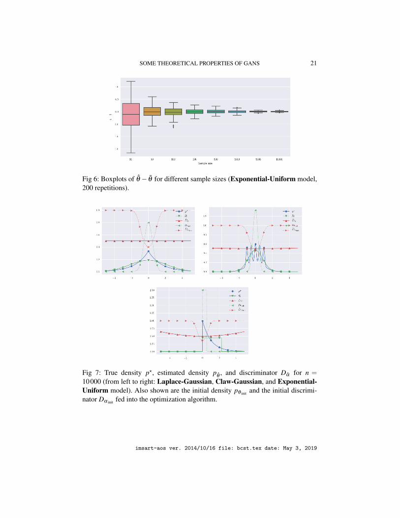
Figure 4 (Laplace-Gaussian), Figure 5 (Claw-Gaussian), and Figure 6 (Expo-nential-Uniform) show the boxplots of the differences θ − θ over 200 repetitions,for a sample size n varying from 10 to 10000. In these experiments, the parameterθ is obtained by averaging the θ for the largest sample size n. In accordance withTheorem 4.2, the size of the boxplots shrinks around 0 when n increases, thusshowing that the estimated parameter θ is getting closer and closer to θ . Beforeanalyzing at which rate this convergence occurs, we may have a look at Figure 7,which plots the estimated density p
θ(for n = 10000) vs. the true density p?. It also
shows the discriminator Dα , together with the initial density pθ init and the initialdiscriminator Dα init fed into the optimization algorithm. We note that in the threemodels, Dα is almost identically 1/2, meaning that it is impossible to discriminatebetween the original observations and those generated by p
θ.
In line with the above, our next step is to state a central limit theorem for θ . Al-though simple to understand, this result requires additional assumptions and some
imsart-aos ver. 2014/10/16 file: bcst.tex date: May 3, 2019

20 G. BIAU ET AL.
Fig 4: Boxplots of θ− θ for different sample sizes (Laplace-Gaussian model, 200repetitions).
Fig 5: Boxplots of θ − θ for different sample sizes (Claw-Gaussian model, 200repetitions).
technical prerequisites. One first needs to ensure that the function (θ ,α) 7→ L(θ ,α)is regular enough in a neighborhood of (θ , α). This is captured by the followingset of assumptions, which require in particular the uniqueness of the maximizer ofthe function α 7→ L(θ ,α) for a θ around θ . For a function F : Θ → R (respec-tively, G : Θ ×Λ → R), we let HF(θ) (respectively, H1G(θ ,α) and H2G(θ ,α))be the Hessian matrix of the function θ 7→ F(θ) (respectively, θ 7→ G(θ ,α) andα 7→ G(θ ,α)) computed at θ (respectively, at θ and α).
imsart-aos ver. 2014/10/16 file: bcst.tex date: May 3, 2019
SOME THEORETICAL PROPERTIES OF GANS 21
Fig 6: Boxplots of θ − θ for different sample sizes (Exponential-Uniform model,200 repetitions).
Fig 7: True density p?, estimated density pθ
, and discriminator Dα for n =10000 (from left to right: Laplace-Gaussian, Claw-Gaussian, and Exponential-Uniform model). Also shown are the initial density pθ init and the initial discrimi-nator Dα init fed into the optimization algorithm.
imsart-aos ver. 2014/10/16 file: bcst.tex date: May 3, 2019

22 G. BIAU ET AL.
Assumptions (Hloc)
(HU) There exists a neighborhood U of θ and a function α : U →Λ such that
argmaxα∈Λ
L(θ ,α) = {α(θ)}, ∀θ ∈U.
(HV ) The Hessian matrix HV (θ) is invertible, where V (θ)def= L(θ ,α(θ)).
(HH) The Hessian matrix H2L(θ , α) is invertible.
We stress that under Assumption (HU), there is for each θ ∈U a unique α(θ) ∈Λ such that L(θ ,α(θ)) = supα∈Λ L(θ ,α). We also note that α(θ) = α under (H1).We still need some notation before we state the central limit theorem. For a functionf (θ ,α), ∇1 f (θ ,α) (respectively, ∇2 f (θ ,α)) means the gradient of the functionθ 7→ f (θ ,α) (respectively, the function α 7→ f (θ ,α)) computed at θ (respectively,at α). For a function g(t), J(g)t is the Jacobian matrix of g computed at t. Observethat by the envelope theorem,
HV (θ) = H1L(θ , α)+ J(∇1L(θ , ·))αJ(α)θ ,
where, by the chain rule,
J(α)θ =−H2L(θ , α)−1J(∇2L(·, α))θ .
Therefore, in Assumption (HV ), the Hessian matrix HV (θ) can be computed withthe sole knowledge of L. Finally, we let
`1(θ ,α) = lnDα(X1)+ ln(1−Dα ◦Gθ (Z1)),
and denote by L→ the convergence in distribution.
THEOREM 4.3. Under Assumptions (H ′reg), (H1), and (Hloc), one has
√n(θ − θ)
L→ Z,
where Z is a Gaussian random variable with mean 0 and covariance matrix
V = Var[−HV (θ)−1
∇1`1(θ , α)+HV (θ)−1J(∇1L(θ , ·))α H2L(θ , α)−1∇2`1(θ , α)
].
The expression of the covariance is relatively complex and, unfortunately, can-not be simplified, even for a dimension of the parameter equal to 1. We note how-ever that if Y is a random vector of Rp whose components are bounded in absolutevalue by some δ > 0, then the Euclidean norm of the covariance matrix of Y isbounded by 4pδ 2. But each component of the random vector of Rp involved in
imsart-aos ver. 2014/10/16 file: bcst.tex date: May 3, 2019

SOME THEORETICAL PROPERTIES OF GANS 23
the covariance matrix V is bounded in absolute value by Cpq2, for some posi-tive constant C resulting from Assumption (H ′reg). We conclude that the Euclideannorm of V is bounded by 4C2 p3q4. Thus, our statistical approach reveals that inthe overparameterized regime (i.e, when p and q are very large compared to n), theestimator θ has a large dispersion around θ , which may affects the performance ofthe algorithm.
Nevertheless, the take-home message of Theorem 4.3 is that the estimator θ isasymptotically normal, with a convergence rate of
√n. This is illustrated in Figures
8, 9, and 10, which respectively show the histograms and kernel estimates of thedistribution of
√n(θ − θ) for the Laplace-Gaussian, the Claw-Gaussian, and the
Exponential-Uniform model in function of the sample size n (200 repetitions).
Fig 8: Histograms and kernel estimates (continuous line) of the distribution of√n(θ − θ) for different sample sizes n (Laplace-Gaussian model, 200 repeti-
tions).
PROOF. By technical Lemma 6.1, we can find under Assumptions (H ′reg) and(H1) an open set V ⊂U ⊂Θ ◦ containing θ such that, for all θ ∈ V , α(θ) ∈ Λ ◦.
imsart-aos ver. 2014/10/16 file: bcst.tex date: May 3, 2019

24 G. BIAU ET AL.
Fig 9: Histograms and kernel estimates (continuous line) of the distribution of√n(θ − θ) for different sample sizes n (Claw-Gaussian model, 200 repetitions).
In the sequel, to lighten the notation, we assume without loss of generality thatV =U . Thus, for all θ ∈U , we have α(θ) ∈Λ ◦ and L(θ ,α(θ)) = supα∈Λ L(θ ,α)(with α(θ) = α by (H1)). Accordingly, ∇2L(θ ,α(θ)) = 0, ∀θ ∈ U . Also, sinceH2L(θ , α) is invertible by (HH) and since the function (θ ,α) 7→H2L(θ ,α) is con-tinuous, there exists an open set U ′ ⊂U such that H2L(θ ,α) is invertible as soonas (θ ,α) ∈ (U ′,α(U ′)). Without loss of generality, we assume that U ′ =U . Thus,by the chain rule, the function α is of class C2 in a neighborhood U ′ ⊂U of θ , sayU ′ =U , with Jacobian matrix given by
J(α)θ =−H2L(θ ,α(θ))−1J(∇2L(·,α(θ))
)θ, ∀θ ∈U.
We note that H2L(θ ,α(θ))−1 is of format q× q and J(∇2L(·,α(θ)))θ of formatq× p.
Now, for each θ ∈U , we let α(θ) be such that L(θ , α(θ)) = supα∈Λ L(θ ,α).
imsart-aos ver. 2014/10/16 file: bcst.tex date: May 3, 2019

SOME THEORETICAL PROPERTIES OF GANS 25
Fig 10: Histograms and kernel estimates (continuous line) of the distribution of√n(θ − θ) for different sample sizes n (Exponential-Uniform model, 200 repeti-
tions).
Clearly,
|L(θ , α(θ))−L(θ ,α(θ))|≤ |L(θ , α(θ))− L(θ , α(θ))|+ |L(θ , α(θ))−L(θ ,α(θ))|≤ sup
α∈Λ
|L(θ ,α)− L(θ ,α)|+ | supα∈Λ
L(θ ,α)− supα∈Λ
L(θ ,α)|
≤ 2 supα∈Λ
|L(θ ,α)−L(θ ,α)|.
Therefore, by Lemma 4.1, supθ∈U |L(θ , α(θ))− L(θ ,α(θ))| → 0 almost surely.The event on which this convergence holds does not depend upon θ ∈ U , and,arguing as in the proof of Theorem 4.2, we deduce that under (H1), P(α(θ)→α(θ)∀θ ∈U)= 1. Since α(θ)∈Λ ◦ for all θ ∈U , we also haveP(α(θ)∈Λ ◦∀θ ∈U)→ 1 as n→∞. Thus, in the sequel, it will be assumed without loss of generalitythat, for all θ ∈U , α(θ) ∈Λ ◦.
imsart-aos ver. 2014/10/16 file: bcst.tex date: May 3, 2019

26 G. BIAU ET AL.
Still by Lemma 4.1, supθ∈Θ ,α∈Λ ‖H2L(θ ,α)−H2L(θ ,α)‖ → 0 almost surely.Since H2L(θ ,α) is invertible on U×α(U), we have
P(H2L(θ ,α) invertible ∀(θ ,α) ∈U×α(U)
)→ 1.
Thus, we may and will assume that H2L(θ ,α) is invertible for all (θ ,α) ∈ U ×α(U).
Next, since α(θ) ∈Λ ◦ for all θ ∈U , one has ∇2L(θ , α(θ)) = 0. Therefore, bythe chain rule, α is of class C2 on U , with Jacobian matrix
J(α)θ =−H2L(θ , α(θ))−1J(∇2L(·, α(θ))
)θ, ∀θ ∈U.
Let V (θ)def= L(θ , α(θ)) = supα∈Λ L(θ ,α). By the envelope theorem, V is of
class C2, ∇V (θ) = ∇1L(θ , α(θ)), and
HV (θ) = H1L(θ , α(θ))+ J(∇1L(θ , ·))α(θ)J(α)θ .
Recall that θ → θ almost surely by Theorem 4.2, so that we may assume thatθ ∈Θ ◦ by (H1). Moreover, we can also assume that θ + t(θ − θ) ∈U , ∀t ∈ [0,1].Thus, by a Taylor series expansion with integral remainder, we have
(4.3) 0 = ∇V (θ) = ∇V (θ)+∫ 1
0HV (θ + t(θ − θ))dt(θ − θ).
Since α(θ) ∈ Λ ◦ and L(θ , α(θ)) = supα∈Λ L(θ ,α), one has ∇2L(θ , α(θ)) = 0.Thus,
0 = ∇2L(θ , α(θ))
= ∇2L(θ ,α(θ))+∫ 1
0H2L
(θ ,α(θ)+ t(α(θ)−α(θ))
)dt(α(θ)−α(θ)).
By Lemma 4.1, since α(θ)→ α(θ) almost surely, we have
I1def=∫ 1
0H2L
(θ ,α(θ)+ t(α(θ)−α(θ))
)dt→ H2L(θ , α) almost surely.
Because H2L(θ , α) is invertible,P(I1 invertible)→ 1 as n→∞. Therefore, we mayassume, without loss of generality, that I1 is invertible. Hence,
(4.4) α(θ)−α(θ) =−I−11 ∇2L(θ ,α(θ)).
Furthermore,
∇V (θ) = ∇1L(θ , α(θ)) = ∇1L(θ ,α(θ))+ I2(α(θ)−α(θ)),
imsart-aos ver. 2014/10/16 file: bcst.tex date: May 3, 2019

SOME THEORETICAL PROPERTIES OF GANS 27
where
I2def=∫ 1
0J(∇1L(θ , ·))
α(θ)+t(α(θ)−α(θ))dt.
By Lemma 4.1, I2 → J(∇1L(θ , ·))α(θ) almost surely. Combining (4.3) and (4.4),we obtain
0 = ∇1L(θ ,α(θ))− I2I−11 ∇2L(θ ,α(θ))+ I3(θ − θ),
where
I3def=∫ 1
0HV (θ + t(θ − θ))dt.
By technical Lemma 6.2, we have I3→ HV (θ) almost surely. So, by (HV ), it canbe assumed that I3 is invertible. Consequently,
θ − θ =−I−13 ∇1L(θ ,α(θ))+ I−1
3 I2I−11 ∇2L(θ ,α(θ)),
or, equivalently, since α(θ) = α ,
θ − θ =−I−13 ∇1L(θ , α)+ I−1
3 I2I−11 ∇2L(θ , α).
Using Lemma 4.1, we conclude that√
n(θ − θ) has the same limit distribution as
Sndef=−√
nHV (θ)−1∇1L(θ , α)+
√nHV (θ)−1J(∇1L(θ , ·))α H2L(θ , α)−1
∇2L(θ , α).
Let`i(θ ,α) = lnDα(Xi)+ ln(1−Dα ◦Gθ (Zi)), 1≤ i≤ n.
With this notation, we have
Sn =1√n
n
∑i=1
(−HV (θ)−1
∇1`i(θ , α)+HV (θ)−1J(∇1L(θ , ·))α H2L(θ , α)−1∇2`i(θ , α)
).
One has ∇V (θ) = 0, since V (θ) = infθ∈Θ V (θ) and θ ∈ Θ ◦. Therefore, under(H ′reg),E∇1`i(θ , α) =∇1E`i(θ , α) =∇1L(θ , α) =∇V (θ) = 0. Similarly, we haveE∇2`i(θ , α)=∇2E`i(θ , α)=∇2L(θ , α)= 0, since L(θ , α)= supα∈Λ L(θ ,α) andα ∈Λ ◦. Using the central limit theorem, we conclude that
√n(θ − θ)
L→ Z,
where Z is a Gaussian random variable with mean 0 and covariance matrix
V = Var[−HV (θ)−1
∇1`1(θ , α)+HV (θ)−1J(∇1L(θ , ·))α H2L(θ , α)−1∇2`1(θ , α)
].
imsart-aos ver. 2014/10/16 file: bcst.tex date: May 3, 2019

28 G. BIAU ET AL.
5. Conclusion and perspectives. In this paper, we have presented a theoreti-cal study of the original Generative Adversarial Networks (GAN) algorithm, whichconsists in building a generative model of an unknown distribution from samplesfrom that distribution. The key idea of the procedure is to simultaneously train thegenerative model (the generators) and an adversary (the discriminators) that triesto distinguish between real and generated samples. We made a small step towardsa better understanding of this generative process by analyzing some optimalityproperties of the problem in terms of Jensen-Shannon divergence in Section 2, andexplored the role of the discriminator family via approximation arguments in Sec-tion 3. Finally, taking a statistical view, we studied in Section 4 some large sampleproperties (convergence and asymptotic normality) of the parameter describing theempirically selected generator. Some numerical experiments were conducted to il-lustrate the results.
The point of view embraced in the article is statistical, in that it takes into ac-count the variability of the data and its impact on the quality of the estimators. Thispoint of view is different from the classical approach encountered in the literatureon GANs, which mainly focuses on the effective computation of the parametersusing optimization procedures. In this sense, our results must be thought of as acomplementary insight. We realize however that the simplified context in whichwe have placed ourselves, as well as some of the assumptions we have made, arequite far from the typical situations in which GANs algorithms are used. Thus,our work should be seen as a first step towards a more realistic understanding ofGANs, and certainly not as a definitive explanation for their excellent practicalperformance. We give below three avenues of theoretical research that we believeshould be explored as a priority.
1. One of the basic assumptions is that the family of densities {pθ}θ∈Θ (asso-ciated with the generators {Gθ}θ∈Θ ) and the unknown density p? are dom-inated by the same measure µ on the same subset E of Rd . In a way, thismeans that we already have some kind of information on the support of p?,which will typically be a manifold in Rd of dimension smaller than d′ (thedimension of Z). Therefore, the random variable Z, the dimension d′ of theso-called latent space Rd′ , and the parametric model {Gθ}θ∈Θ should becarefully tuned in order to match this constraint. From a practical perspec-tive, the original article of Goodfellow et al. (2014) suggests using for Z auniform or Gaussian distribution of small dimension, without further inves-tigation. Mirza and Osindero (2014) and Radford et al. (2016), who havesurprisingly good practical results with a deep convolutional generator, bothuse a 100-dimensional uniform distribution to represent respectively 28×28and 64×64 pixel images. Many papers have been focusing on either decom-posing the latent space Rd′ to force specified portions of this space to corre-
imsart-aos ver. 2014/10/16 file: bcst.tex date: May 3, 2019

SOME THEORETICAL PROPERTIES OF GANS 29
spond to different variations (as, e.g., in Donahue et al., 2018) or invertingthe generators (e.g., Lipton and Tripathi, 2017; Srivastava et al., 2017; Bo-janowski et al., 2018). However, to the best of our knowledge, there is todate no theoretical result tackling the impact of d′ and Z on the performanceof GANs, and it is our belief that a thorough mathematical investigation ofthis issue is needed for a better understanding of the generating process.Similarly, whenever the {Gθ}θ∈Θ are neural networks, the link between thenetworks (number of layers, dimensionality of Θ , etc.) and the target p?
(support, dominating measure, etc.) is also a fundamental question, whichshould be addressed at a theoretical level.
2. Assumptions (Hε) and (H ′ε) highlight the essential role played by the dis-criminators to approximate the optimal functions D?
θ. We believe that this
point is critical for the theoretical analysis of GANs, and that it should befurther developed in the context of neural networks, with a potentially largenumber of hidden layers.
3. Theorem 4.2 (convergence of the estimated parameter) and Theorem 4.3(asymptotic normality) hold under the assumption that the model is iden-tifiable (uniqueness of θ and α). This identifiability assumption is hardlysatisfied in the high-dimensional context of (deep) neural networks, wherethe function to be optimized displays a very wild landscape, without imme-diate convexity or concavity. Thus, to take one more step towards a morerealistic model, it would be interesting to shift the parametric point of viewand move towards results concerning the convergence of distributions notparameters.
6. Technical results.
6.1. Proof of Theorem 3.1. Let ε ∈ (0,1/(2M)), m ∈ (0,1/2), and D ∈ D besuch that m≤ D≤ 1−m and ‖D−D?
θ‖2 ≤ ε . Observe that
L(θ ,D) =∫
ln(D)p?dµ +∫
ln(1−D)pθ dµ
=∫
ln( D
D?θ
)p?dµ +
∫ln( 1−D
1−D?θ
)pθ dµ +2DJS(p?, pθ )− ln4.(6.1)
We first derive a lower bound on the quantity
I def=∫
ln( D
D?θ
)p?dµ +
∫ln( 1−D
1−D?θ
)pθ dµ
=∫
ln(D(p?+ pθ )
p?
)p?dµ +
∫ln((1−D)(p?+ pθ )
pθ
)pθ dµ.
imsart-aos ver. 2014/10/16 file: bcst.tex date: May 3, 2019

30 G. BIAU ET AL.
Let dP? = p?dµ , dPθ = pθ dµ ,
dκ =D(p?+ pθ )∫D(p?+ pθ )dµ
dµ, and dκ′ =
(1−D)(p?+ pθ )∫(1−D)(p?+ pθ )dµ
dµ.
Observe, since m ≤ D ≤ 1−m, that P?� κ and Pθ � κ ′. With this notation, wehave
I =−DKL(P? ‖ κ)−DKL(Pθ ‖ κ′)
+ ln[∫
D(p?+ pθ )dµ(2−
∫D(p?+ pθ )dµ
)].(6.2)
Since ∫D(p?+ pθ )dµ =
∫(D−D?
θ)(p?+ pθ )dµ +1,
the Cauchy-Schwartz inequality leads to∣∣∣∫ D(p?+ pθ )dµ−1∣∣∣≤ ‖D−D?
θ‖2‖p?+ pθ‖2
≤ 2Mε,(6.3)
because both p? and pθ are bounded by M. Thus,
ln[∫
D(p?+ pθ )dµ(2−
∫D(p?+ pθ )dµ
)]≥ ln(1−4M2
ε2)
≥− 4M2ε2
1−4M2ε2 ,(6.4)
using the inequality ln(1− x)≥−x/(1− x) for x ∈ [0,1). Moreover, recalling thatthe Kullback-Leibler divergence is smaller than the chi-square divergence, and let-ting F = F/(
∫Fdµ) for F ∈ L1(µ), we have
DKL(P? ‖ κ)≤∫ ( p?
D(p?+ pθ )−1)2
D(p?+ pθ )dµ.
Hence, letting J def=∫
D(p?+ pθ )dµ , we see that
DKL(P? ‖ κ)
≤ 1J
∫ (p?∫
D(p?+ pθ )dµ−D(p?+ pθ ))2 1
D(p?+ pθ )dµ
=1J
∫ (p?∫(D−D?
θ)(p?+ pθ )dµ +(D?
θ−D)(p?+ pθ )
)2 1D(p?+ pθ )
dµ.
imsart-aos ver. 2014/10/16 file: bcst.tex date: May 3, 2019

SOME THEORETICAL PROPERTIES OF GANS 31
Since ε < 1/(2M), inequality (6.3) gives 1/J ≤ c1 for some constant c1 > 0. ByCauchy-Schwarz and (a+b)2 ≤ 2(a2 +b2), we obtain
DKL(P? ‖ κ)
≤ 2c1
(∫ (∫(D−D?
θ)(p?+ pθ )dµ
)2 (p?)2
D(p?+ pθ )dµ +
∫(D?
θ−D)2 p?+ pθ
Ddµ
)≤ 2c1
(‖D−D?
θ‖2
2‖p?+ pθ‖22
∫(p?)2
D(p?+ pθ )dµ +
∫(D?
θ−D)2 p?+ pθ
Ddµ
).
Therefore, since p? ≤M, pθ ≤M, and D≥ m,
DKL(P? ‖ κ)≤ 2c1
(4M2
m+
2Mm
)ε
2.
One proves with similar arguments that
DKL(Pθ ‖ κ′)≤ 2c1
(4M2
m+
2Mm
)ε
2.
Combining these two inequalities with (6.2) and (6.4), we see that I ≥ −c2ε2 forsome constant c2 > 0 that depends only upon M and m. Getting back to identity(6.1), we conclude that
2DJS(p?, pθ )≤ c2ε2 +L(θ ,D)+ ln4.
But
L(θ ,D)≤ supD∈D
L(θ ,D)≤ supD∈D
L(θ ?,D)
(by definition of θ )
≤ supD∈D∞
L(θ ?,D)
= L(θ ?,D?θ ?) = 2DJS(p?, pθ ?)− ln4.
Thus,2DJS(p?, pθ )≤ c2ε
2 +2DJS(p?, pθ ?).
This shows the right-hand side of inequality (3.1). To prove the left-hand side, justnote that by inequality (2.2),
DJS(p?, pθ ?)≤ DJS(p?, pθ ).
imsart-aos ver. 2014/10/16 file: bcst.tex date: May 3, 2019

32 G. BIAU ET AL.
6.2. Proof of Lemma 4.1. To simplify the notation, we set
∆ =∂ a+b+c+d
∂θ ai ∂θ b
j ∂αc` ∂αd
m.
Using McDiarmid’s inequality (McDiarmid, 1989), we see that there exists a con-stant c > 0 such that, for all ε > 0,
P(∣∣∣ sup
θ∈Θ ,α∈Λ
|∆ L(θ ,α)−∆L(θ ,α)|−E supθ∈Θ ,α∈Λ
|∆ L(θ ,α)−∆L(θ ,α)|∣∣∣≥ ε
)≤ 2e−cnε2
.
Therefore, by the Borel-Cantelli lemma,
(6.5) supθ∈Θ ,α∈Λ
|∆ L(θ ,α)−∆L(θ ,α)|−E supθ∈Θ ,α∈Λ
|∆ L(θ ,α)−∆L(θ ,α)| → 0
almost surely. It is also easy to verify that under Assumptions (H ′reg), the process(∆ L(θ ,α)−∆L(θ ,α))θ∈Θ ,α∈Λ is subgaussian. Thus, as in the proof of Theorem4.1, we obtain via Dudley’s inequality that
(6.6) E supθ∈Θ ,α∈Λ
|∆ L(θ ,α)−∆L(θ ,α)|= O( 1√
n
),
since E∆ L(θ ,α) = ∆L(θ ,α). The result follows by combining (6.5) and (6.6).
6.3. Some technical lemmas.
LEMMA 6.1. Under Assumptions (H ′reg) and (H1), there exists an open setV ⊂Θ ◦ containing θ such that, for all θ ∈V , argmaxα∈Λ L(θ ,α)∩Λ ◦ 6= /0.
PROOF. Assume that the statement is not true. Then there exists a sequence(θk)k⊂Θ such that θk→ θ and, for all k, αk ∈ ∂Λ , where αk ∈ argmaxα∈ΛL(θk,α).Thus, since Λ is compact, even if this means extracting a subsequence, one hasαk→ z ∈ ∂Λ as k→ ∞. By the continuity of L, L(θ ,αk)→ L(θ ,z). But
|L(θ ,αk)−L(θ , α)| ≤ |L(θ ,αk)−L(θk,αk)|+ |L(θk,αk)−L(θ , α)|≤ sup
α∈Λ
|L(θ ,α)−L(θk,α)|+ | supα∈Λ
L(θk,α)− supα∈Λ
L(θ ,α)|
≤ 2 supα∈Λ
|L(θ ,α)−L(θk,α)|,
which tends to zero as k→∞ by (H ′D) and (H ′p). Therefore, L(θ ,z) = L(θ , α) and,in turn, z = α by (H1). Since z ∈ ∂Λ and α ∈Λ ◦, this is a contradiction.
LEMMA 6.2. Under Assumptions (H ′reg), (H1), and (Hloc), one has I3→HV (θ)almost surely.
imsart-aos ver. 2014/10/16 file: bcst.tex date: May 3, 2019

SOME THEORETICAL PROPERTIES OF GANS 33
PROOF. We have
I3 =∫ 1
0HV (θ + t(θ − θ))dt =
∫ 1
0
(H1L(θt , α(θt))+ J(∇1L(θt , ·))α(θt)
J(α)θt
)dt,
where we set θt = θ + t(θ − θ). Note that θt ∈U for all t ∈ [0,1]. By Lemma 4.1,
supt∈[0,1]
‖H1L(θt , α(θt))−H1L(θt , α(θt))‖
≤ supθ∈Θ ,α∈Λ
‖H1L(θ ,α)−H1L(θ ,α)‖→ 0 almost surely.
Also, by Theorem 4.2, for all t ∈ [0,1], θt → θ almost surely. Besides,
|L(θ , α(θt))−L(θ ,α(θ))| ≤ |L(θ , α(θt))−L(θt , α(θt))|+ |L(θt , α(θt))−L(θ ,α(θ))|≤ sup
α∈Λ
|L(θ ,α)−L(θt ,α)|
+2 supθ∈Θ ,α∈Λ
|L(θ ,α)−L(θ ,α)|.
Thus, via (H ′reg), (H1), and Lemma 4.1, we conclude that almost surely, for allt ∈ [0,1], one has α(θt)→ α(θ) = α . Accordingly, almost surely, for all t ∈ [0,1],H1L(θt , α(θt))→ H1L(θ , α). Since H1L(θ ,α) is bounded under (H ′D) and (H ′p),the Lebesgue dominated convergence theorem leads to
(6.7)∫ 1
0H1L(θt , α(θt))dt→ H1L(θ , α) almost surely.
Furthermore,
J(α)θ =−H2L(θ , α(θ))−1J(∇2L(·, α(θ))
)θ, ∀(θ ,α) ∈U×α(U),
where U is the open set defined in the proof of Theorem 4.3. By the cofactormethod, H2L(θ ,α)−1 takes the form
H2L(θ ,α)−1 =c(θ ,α)
det(H2L(θ ,α)),
where c(θ ,α) is the matrix of cofactors associated with H2L(θ ,α). Thus, eachcomponent of −H2L(θ ,α)−1J(∇2L(·,α))θ is a quotient of a multilinear form ofthe partial derivatives of L evaluated at (θ ,α) divided by det(H2L(θ ,α)), which isitself a multilinear form in the ∂ 2L
∂αi∂α j(θ ,α). Hence, by Lemma 4.1, we have
supθ∈U,α∈α(U)
‖H2L(θ ,α)−1J(∇2L(·,α))θ −H2L(θ ,α)−1J(∇2L(·,α))θ‖→ 0
imsart-aos ver. 2014/10/16 file: bcst.tex date: May 3, 2019

34 G. BIAU ET AL.
almost surely. So, for all n large enough,
supt∈[0,1]
‖J(α)θt+H2L(θt , α(θt))
−1J(∇2L(·, α(θt))
)θt‖
≤ supθ∈U,α∈α(U)
‖H2L(θ ,α)−1J(∇2L(·,α))θ −H2L(θ ,α)−1J(∇2L(·,α))θ‖
→ 0 almost surely.
We know that almost surely, for all t ∈ [0,1], α(θt)→ α . Thus, since the functionU ×α(U) 3 (θ ,α) 7→ H2L(θ ,α)−1J(∇2L(·,α))θ is continuous, we have almostsurely, for all t ∈ [0,1],
H2L(θt , α(θt))−1J(∇2L(·, α(θt))
)θt→ H2L(θ , α)−1J(∇2L(·, α))θ .
Therefore, almost surely, for all t ∈ [0,1], J(α)θt→ J(α)θ . Similarly, almost surely,
for all t ∈ [0,1], J(∇1L(θt , ·))α(θt)→ J(∇1L(θ , ·))α . All involved quantities are
uniformly bounded in t, and so, by the Lebesgue dominated convergence theorem,we conclude that
(6.8)∫ 1
0J(∇1L(θt , ·))α(θt)
J(α)θt
dt→ J(∇1L(θ , ·))αJ(α)θ almost surely.
Consequently, by combining (6.7) and (6.8),
I3→ H1L(θ , α)+ J(∇1L(θ , ·))αJ(α)θ = HV (θ) almost surely,
as desired.
ACKNOWLEDGEMENTS
We thank Flavian Vasile (Criteo AI Lab) and Antoine Picard-Weibel (ENS Ulm)for stimulating discussions and insightful suggestions. We also thank the AssociateEditor and two anonymous referees for their careful reading of the paper and con-structive comments, which led to a substantial improvement of the document.
REFERENCES
M. Abadi, A. Agarwal, P. Barham, E. Brevdo, Z. Chen, C. Citro, G.S. Corrado, A. Davis, J. Dean,M. Devin, S. Ghemawat, I. Goodfellow, A. Harp, G. Irving, M. Isard, Y. Jia, R. Jozefowicz,L. Kaiser, M. Kudlur, J. Levenberg, D. Mane, R. Monga, S. Moore, D. Murray, C. Olah, M. Schus-ter, J. Shlens, B. Steiner, I. Sutskever, K. Talwar, P. Tucker, V. Vanhoucke, V. Vasudevan, F. Viegas,O. Vinyals, P. Warden, M. Wattenberg, M. Wicke, Y. Yu, and X. Zheng. TensorFlow: A system forlarge-scale machine learning, 2015. URL https://www.tensorflow.org/. Software availablefrom tensorflow.org.
T. Angles and S. Mallat. Generative networks as inverse problems with scattering transforms. InInternational Conference on Learning Representations, 2018.
imsart-aos ver. 2014/10/16 file: bcst.tex date: May 3, 2019

SOME THEORETICAL PROPERTIES OF GANS 35
M. Arjovsky and L. Bottou. Towards principled methods for training generative adversarial networks.In International Conference on Learning Representations, 2017.
M. Arjovsky, S. Chintala, and L. Bottou. Wasserstein generative adversarial networks. In D. Precupand Y. Whye Teh, editors, Proceedings of the 34th International Conference on Machine Learn-ing, volume 70, pages 214–223. Proceedings of Machine Learning Research, 2017.
P. Bojanowski, A. Joulin, D. Lopez-Paz, and A. Szlam. Optimizing the latent space of generativenetworks. In J. Dy and A. Krause, editors, Proceedings of the 35th International Conferenceon Machine Learning, volume 80, pages 600–609. Proceedings of Machine Learning Research,2018.
L. Devroye. Universal smoothing factor selection in density estimation: Theory and practice. TEST,6:223–320, 1997.
C. Donahue, Z.C. Lipton, A. Balsubramani, and J. McAuley. Semantically decomposing the latentspaces of generative adversarial networks. In International Conference on Learning Representa-tions, 2018.
G.K. Dziugaite, D.M. Roy, and Z. Ghahramani. Training generative neural networks via maximummean discrepancy optimization. In M. Meila and T. Heskes, editors, Proceedings of the Thirty-First Conference on Uncertainty in Artificial Intelligence, pages 258–267. AUAI Press, Arlington,2015.
D.M. Endres and J.E. Schindelin. A new metric for probability distributions. IEEE Transactions onInformation Theory, 49:1858–1860, 2003.
I. Goodfellow. NIPS 2016 Tutorial: Generative Adversarial Networks. arXiv:1701.00160, 2016.I. Goodfellow, J. Pouget-Abadie, M. Mirza, B. Xu, D. Warde-Farley, S. Ozair, A. Courville, and
J. Bengio. Generative adversarial nets. In Z. Ghahramani, M. Welling, C. Cortes, N.D. Lawrence,and K.Q. Weinberger, editors, Advances in Neural Information Processing Systems 27, pages2672–2680. Curran Associates, Inc., Red Hook, 2014.
T. Liang. On how well generative adversarial networks learn densities: Nonparametric and para-metric results. arXiv:1811.03179, 2018.
Z.C. Lipton and S. Tripathi. Precise recovery of latent vectors from generative adversarial networks.arxiv:1702.04782, 2017.
S. Liu, O. Bousquet, and K. Chaudhuri. Approximation and convergence properties of generativeadversarial learning. In I. Guyon, U.V. Luxburg, S. Bengio, H. Wallach, R. Fergus, S. Vish-wanathan, and R. Garnett, editors, Advances in Neural Information Processing Systems 30, pages5551–5559. Curran Associates, Inc., Red Hook, 2017.
C. McDiarmid. On the method of bounded differences. In J. Siemons, editor, Surveys in Com-binatorics, London Mathematical Society Lecture Note Series 141, pages 148–188. CambridgeUniversity Press, Cambridge, 1989.
M. Mirza and S. Osindero. Conditional generative adversarial nets. arXiv:1411.1784, 2014.S. Nowozin, B. Cseke, and R. Tomioka. f-GAN: Training generative neural samplers using varia-
tional divergence minimization. In D.D. Lee, M. Sugiyama, U.V. Luxburg, I. Guyon, and R. Gar-nett, editors, Advances in Neural Information Processing Systems 29, pages 271–279. CurranAssociates, Inc., Red Hook, 2016.
A. Radford, L. Metz, and S. Chintala. Unsupervised representation learning with deep convolutionalgenerative adversarial networks. In International Conference on Learning Representations, 2016.
T. Salimans, I. Goodfellow, W. Zaremba, V. Cheung, A. Radford, and X. Chen. Improved techniquesfor training GANs. In D.D. Lee, M. Sugiyama, U.V. Luxburg, I. Guyon, and R. Garnett, editors,Advances in Neural Information Processing Systems 29, pages 2234–2242. Curran Associates,Inc., Red Hook, 2016.
A. Srivastava, L. Valkoz, C. Russell, M.U. Gutmann, and C. Sutton. Veegan: Reducing mode collapsein GANs using implicit variational learning. In I. Guyon, U.V. Luxburg, S. Bengio, H. Wallach,R. Fergus, S. Vishwanathan, and R. Garnett, editors, Advances in Neural Information Processing
imsart-aos ver. 2014/10/16 file: bcst.tex date: May 3, 2019

36 G. BIAU ET AL.
Systems 30, pages 3308–3318. Curran Associates, Inc., Red Hook, 2017.R. van Handel. Probability in High Dimension. APC 550 Lecture Notes, Princeton University, 2016.P. Zhang, Q. Liu, D. Zhou, T. Xu, and X. He. On the discriminative-generalization tradeoff in GANs.
In International Conference on Learning Representations, 2018.
G. BIAUM. SANGNIERSORBONNE UNIVERSITELABORATOIRE DE PROBABILITES,STATISTIQUE ET MODELISATIONBOITE 158, TOUR 15-254 PLACE JUSSIEU75005 PARIS, FRANCEE-MAIL: [email protected]
B. CADREUNIV RENNES, IRMARENS RENNESAVENUE ROBERT SCHUMANN35170 BRUZ, FRANCEE-MAIL: [email protected]
U. TANIELIANCRITEO AI LAB32 RUE BLANCHE75009 PARIS, FRANCEE-MAIL: [email protected]
imsart-aos ver. 2014/10/16 file: bcst.tex date: May 3, 2019