sound wave interference - rutgers physics & astronomythe two ends of a guitar string do not...
TRANSCRIPT
7/06 Sound Wave Interference
Sound Wave Interference
About this lab
Interference is the hallmark of classical wave phenomena, and also of quantum mechanical waves. Classical examples include sound waves in fluids (longitudinal only) or in solids (longitudinal and transverse), football spectator demonstrations, radio waves, etc.
Essential to understanding persistent interference is understanding the concept of relative phase between two or more waves of the same frequency (and thus of the same wavelength), and of relative amplitudes of the two waves. With identical amplitudes, the net amplitude can range from twice that of either to zero, depending on relative phase. With different amplitudes (for instance, with two unbalanced speakers), the range is from the sum to the difference.
And the relative phase will vary from point to point in space, due to differences in travel distance and, in addition, to any non-zero initial phase relation between the two sources.. You will observe the corresponding intensity variation, where intensity is proportional to the square of the net amplitude.
Apparatus: Computer, stereo speakers, microphone, meter stick, masking tape, FFTScope, Beats, Interference
References: Cutnell & Johnson: Physics 6th Ed. Chapter 17Serway & Beichner: Physics for Scientists & Engineers v2, 5th Ed. Ch. 18: Example 18.1, Section 18.7
Introduction:
Sound waves are disturbances in a medium that propagate from one place to another, without the actual transport of the particles that make up the wave. For instance, a sound wave traveling from a loudspeaker to your ear results in the successive compression and rarefaction of molecules of air between the loudspeaker and your ear, the molecules moving in the direction of wave propagation. But the molecules themselves are not transported any appreciable distance. In contrast, a breeze blowing on a warm summer day involves mass transport of air molecules, rather than wave motion.
(A wind of 100 km/hour involves mass motion of only about 28 m/s, whereas random thermal velocities of air molecules at 200 C are 478 m/s (N2) and 511 m/s (O2), and the
7/06 Sound Wave Interference
propagation velocity of a sound wave in air is 343 m/s (200 C), comparable to the thermal velocities.)
In a fluid only longitudinal waves can occur (it is not possible to shake a fluid sideways). But in a solid, both longitudinal and transverse modes (sideways motion of the individual particles) occur. Earthquakes (or underground nuclear tests) generate both types, which propagate with different velocities, which also vary with the depth (i.e. with density and composition). These waves provide the only probe of the earth's interior and lead to our knowledge of a liquid nickel-iron region in the deep interior.
When waves interact with each other, especially waves of the same (or nearly the same) frequency and phase, interesting effects occur.
Beats result from combining at a point in space (e.g., your eardrum) two waves of different frequency. They are a periodic slow temporal variation (modulation) in the amplitude of the resulting wave, with periodic slow temporal variation in the perceived loudness, at twice the slow amplitude modulation frequency. In more detail:
Consider two waves of separate amplitudes y1 = y0sin( 1 t ) and y2= y0sin (2 t ) . Their sum amplitude (after trigonometric manipulation) is exactly
y = ( y1+ y2 )= 2y0cos [ (1 -2
2) t ] * sin [ (
1 +2
2) t ]
The sine term represents a wave with angular frequency 1+2
2 , the average of
1 and 2 . (Remember: “angular” frequency = 2 f saves writing 2π's.)
The cosine term represents a maximum amplitude envelope, oscillating at slow (angular)
frequency 1 -2
2. (To see this, follow the smooth cosine curve of amplitude
modulation - no sudden changes of slope!) However, since energy is proportional to the square of the amplitude (maxima or minima), the perceived audible (angular) frequency of the intensity maxima is
1 -2 , the difference of 1 and 2 (the energy peaks twice each amplitude cycle).
Spatial interference is detected whenever there is a difference in the source-receiver path
7/06 Sound Wave Interference
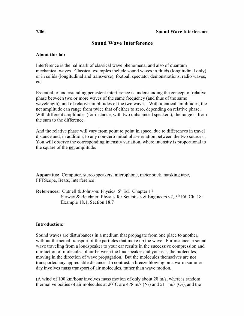
lengths r2 and r1, from two wave sources (2 and 1) of the same frequency (with additional contribution from any initial phase difference). This results in the two wave phases verying, depending on the point of observation. At one point, the resulting intensity may be less than that of either wave separately; at another, more. For two waves in phase to interfere completely constructively (maximum net amplitude and intensity), the path difference δ (from the two sources to the observation point) must equal an integral number of whole wavelengths:
δ = (r2 – r1) = mλ m = 0,1,2....
(This assumes the two sources emit in phase; if not, adjustment must be made to the above relation.)
Figure 1 Loci of interference maxima and minima for circular (or cylindrical) waves spreading from sources 1 and 2. Straight (red) paths from each source to a particular observation point (up, left) are shown. That observation point lies on a (blue) hyperbola (constant path difference) for which the path difference is 3/2 wavelengths – thus the two waves have 1800 ( π radians) relative phase and their amplitudes will cancel completely provided:
7/06 Sound Wave Interference
a) the sources emit in phase, and
b) the sources emit with the same amplitude.
At many wavelengths from the sources, the hyperbola approaches a straight line. The red hyperbolae represent points of spatial maximum amplitude; in between the red and blue hyperbolae there is a definite phase and consequent definite net amplitude (and corresponding intensity) which is neither a maximum, nor a minimum.
Exact expression for maxima:
δ = (r2 – r1) = mλ m = 0,1,2.... (sources driven in phase)
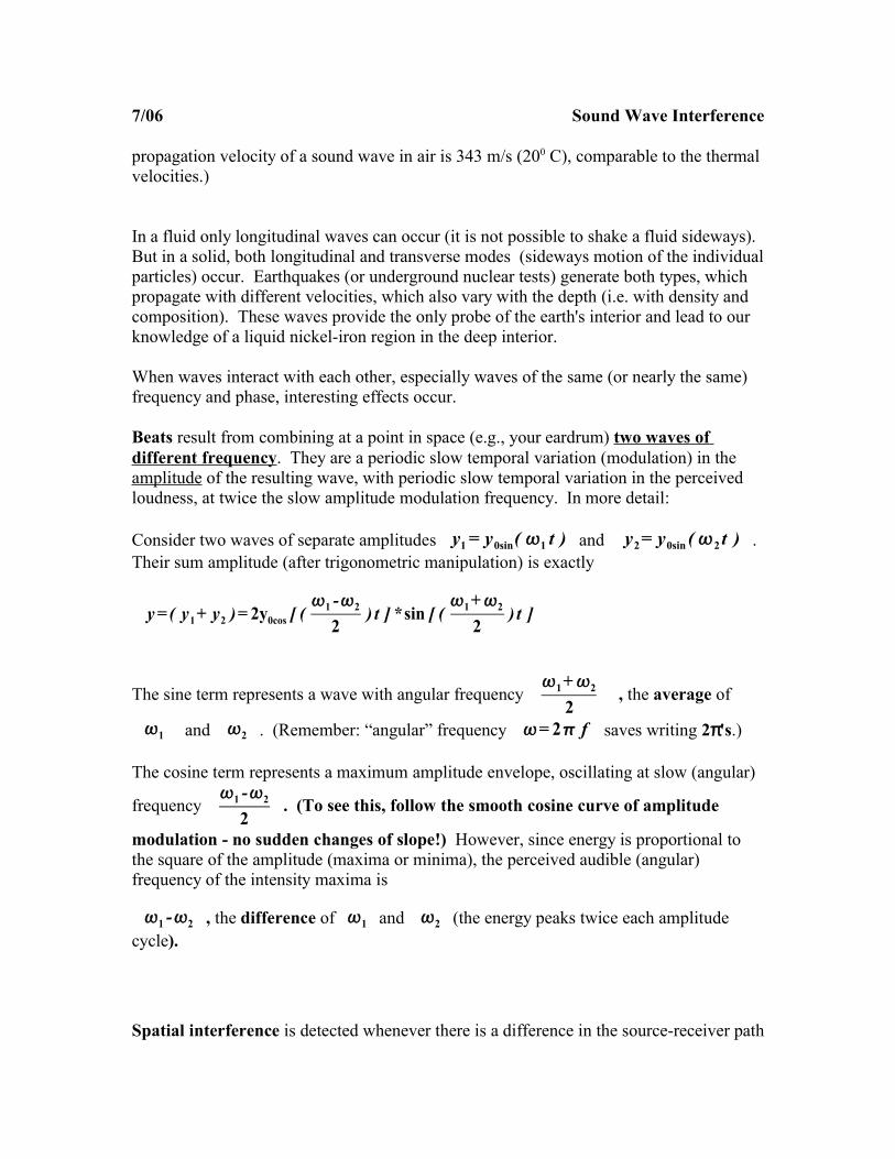
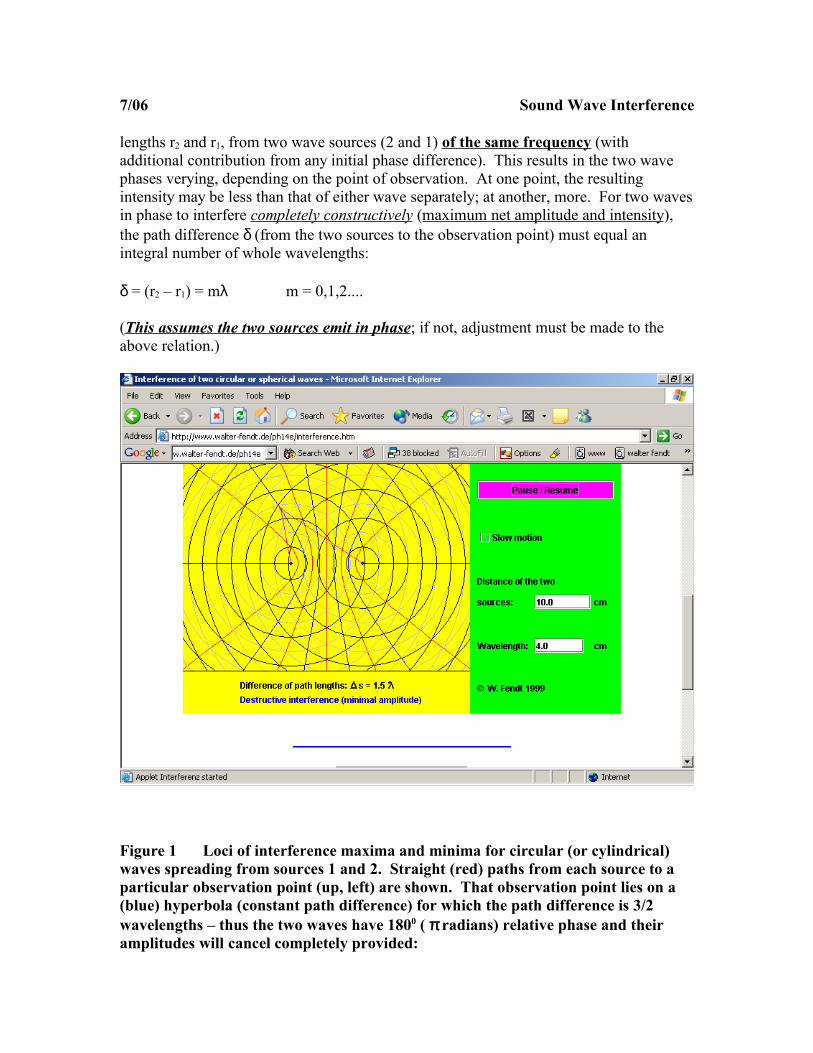
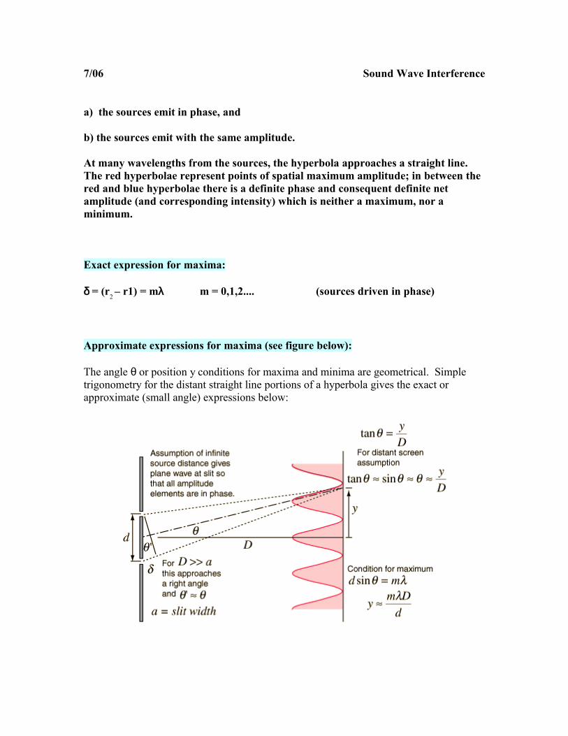
Approximate expressions for maxima (see figure below):
The angle θ or position y conditions for maxima and minima are geometrical. Simple trigonometry for the distant straight line portions of a hyperbola gives the exact or approximate (small angle) expressions below:

7/06 Sound Wave Interference
Figure 2 Geometrical conditions for two-source interference maxima (sources driven in phase)
If r 1 and r 2 (distances from sources 1 and 2 to observation point) are many wavelengths, the fundamental governing quantity (r2 – r1) may be expressed to good approximation, in terms of the wavelength λ (= v/f) and the angle θ, as:
r2 - r1 = d sin , where d is the separation between the two sources, so
Angle maximum:
sin ( max )= md
(m an integer, many wavelengths)
Angle minimum: sin( θ min) = (m + ½)λ/d or
sin ( min )= ( m+ 12
)d
Spatial maximum:
ymax = D tan ( max )≈D sin ( max )= m Dd (small angles, many wavelengths)
Spatial minimum:
ymin = D tan ( min )≈D sin ( min )= [ ( m+ 12
) ] Dd
For small angles, tan(θ) ~ sin(θ) ~ θ (in radians), where 360 0 = 2 π radians.
A particular example of interference.
Standing waves, are typically produced by a single source + boundary reflections. They occur when a wave interferes with itself (single source). They typically consist of two counter-traveling waves, one directed away from the driving source, the other toward it, due to reflection Standing waves are characterized by the boundary conditions that define the state of the wave at the ends of a limited region. (See Figure 3.) For example, the two ends of a guitar string do not move; we call these two points nodes. In contrast,
7/06 Sound Wave Interference
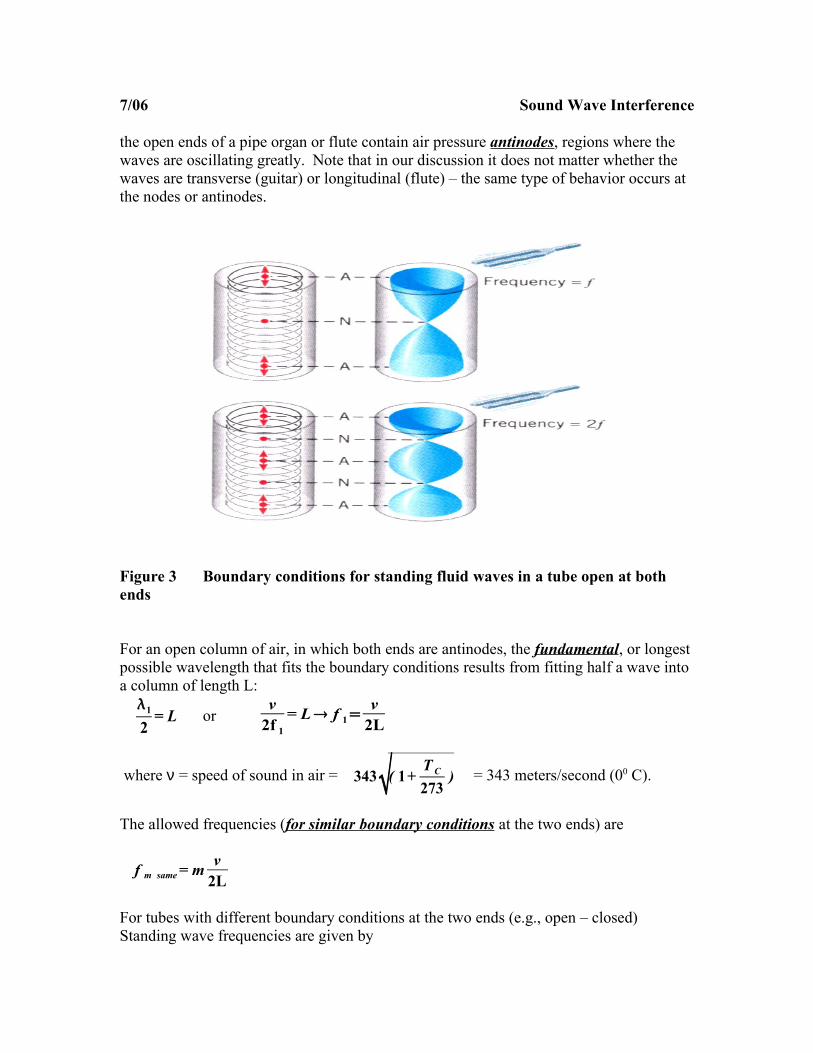
the open ends of a pipe organ or flute contain air pressure antinodes, regions where the waves are oscillating greatly. Note that in our discussion it does not matter whether the waves are transverse (guitar) or longitudinal (flute) – the same type of behavior occurs at the nodes or antinodes.
Figure 3 Boundary conditions for standing fluid waves in a tube open at both ends
For an open column of air, in which both ends are antinodes, the fundamental, or longest possible wavelength that fits the boundary conditions results from fitting half a wave into a column of length L:
1
2= L or
v2f 1
= L f 1=v
2L
where ν = speed of sound in air = 343( 1+T C
273) = 343 meters/second (00 C).
The allowed frequencies (for similar boundary conditions at the two ends) are
f m same = m v2L
For tubes with different boundary conditions at the two ends (e.g., open – closed)Standing wave frequencies are given by

7/06 Sound Wave Interference
f m diff = ( 2m1 ) v4L ;where m = 1,2,3,... , i.e., an odd number of
quarter waves.
Procedure
We will use Beats, FFTScope and Interference.exe, programs that control the PC's sound card to generate various forms, to produce interfering waves from two spatially separated speakers driven by a single oscillator. FFTScope doubles as an oscilloscope/spectrum analyzer; we will also use it to observe the net wave produced at a point by the two interfering traveling speaker waves. As discussed, the relative phase of the two traveling waves at the observation point will determine the net amplitude.
This phase will vary with time at fixed observation point , if the two sources are driven at different sinusoidal frequencies by the Beats program. And the relative phase will vary with space at varying observation points if the two sources are driven at the same sinusoidal frequency by either of the FFTScope Function Generator (zero relative phase) or the Interference (variable relative phase) programs.
The main functions of FFTScope are function generation (FG), oscilloscope (time display) and spectrum analyzer (frequency display). An oscilloscope plots the amplitude (Y-axis) of a waveform vs. time (X-axis). A spectrum analyzer plots the sine/cosine wave amplitude (Y-axis) vs. frequency ( X-axis). To summarize, an oscilloscope shows the waveforms as function of time, while a spectrum analyzer shows the relative importance of the frequencies present in the waveforms. Figure 4 below shows the most commonly used buttons in FFTScope:
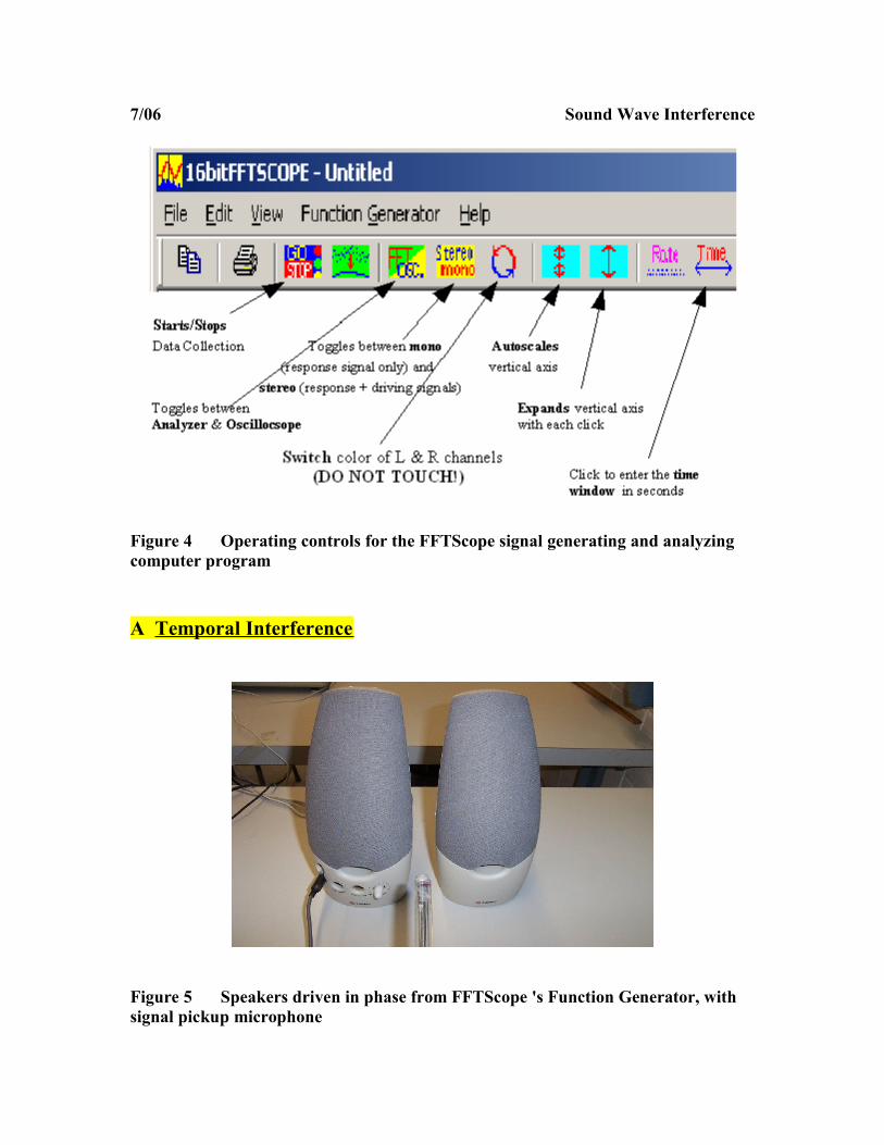
7/06 Sound Wave Interference
Figure 4 Operating controls for the FFTScope signal generating and analyzing computer program
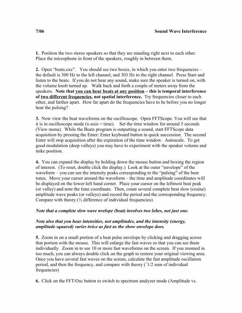
A Temporal Interference
Figure 5 Speakers driven in phase from FFTScope 's Function Generator, with signal pickup microphone
7/06 Sound Wave Interference
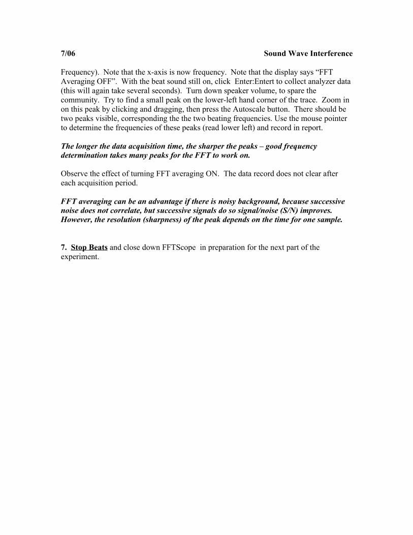
1. Position the two stereo speakers so that they are standing right next to each other. Place the microphone in front of the speakers, roughly in between them.
2. Open “beats.exe”. You should see two boxes, in which you enter two frequencies – the default is 300 Hz to the left channel, and 303 Hz to the right channel. Press Start and listen to the beats. If you do not hear any sound, make sure the speaker is turned on, with the volume knob turned up. Walk back and forth a couple of meters away from the speakers. Note that you can hear beats at any position – this is temporal interference of two different frequencies, not spatial interference. Try frequencies closer to each other, and farther apart. How far apart do the frequencies have to be before you no longer hear the pulsing?
3. Now view the beat waveforms on the oscilloscope. Open FFTScope. You will see that it is in oscilloscope mode (x-axis = time). Set the time window for around 5 seconds (View menu). While the Beats program is outputting a sound, start FFTScope data acquisition by pressing the Enter: Enter keyboard button in quick succession. The second Enter will stop acquisition after the expiration of the time window. Autoscale. To get good modulation (deep valleys) you may have to experiment with the speaker volume and mike position.
4. You can expand the display by holding down the mouse button and boxing the region of interest. (To reset, double click the display.) Look at the outer “envelope” of the waveform – you can see the intensity peaks corresponding to the “pulsing” of the beat tones. Move your cursor around the waveform – the time and amplitude coordinates will be displayed on the lower-left hand corner. Place your cursor on the leftmost beat peak (or valley) and note the time coordinate. Then, count several complete beat slow (cosine) amplitude wave peaks (or valleys) and record the period and the corresponding frequency. Compare with theory (½ difference of individual frequencies).
Note that a complete slow wave nvelope (beat) involves two lobes, not just one.
Note also that you hear intensities, not amplitudes, and the intensity (energy, amplitude squared) varies twice as fast as the show envelope does.
5. Zoom in on a small portion of a beat pulse envelope by clicking and dragging across that portion with the mouse. This will enlarge the fast waves so that you can see them individually. Zoom in to see 10 or more fast waveforms on the screen. If you zoomed in too much, you can always double click on the graph to restore your original viewing area. Once you have several fast waves on the screen, calculate the fast amplitude oscillation period, and then the frequency, and compare with theory (`1/2 sum of individual frequencies)
6. Click on the FFT/Osc button to switch to spectrum analyzer mode (Amplitude vs.
7/06 Sound Wave Interference
Frequency). Note that the x-axis is now frequency. Note that the display says “FFT Averaging OFF”. With the beat sound still on, click Enter:Entert to collect analyzer data (this will again take several seconds). Turn down speaker volume, to spare the community. Try to find a small peak on the lower-left hand corner of the trace. Zoom in on this peak by clicking and dragging, then press the Autoscale button. There should be two peaks visible, corresponding the the two beating frequencies. Use the mouse pointer to determine the frequencies of these peaks (read lower left) and record in report.
The longer the data acquisition time, the sharper the peaks – good frequency determination takes many peaks for the FFT to work on.
Observe the effect of turning FFT averaging ON. The data record does not clear after each acquisition period.
FFT averaging can be an advantage if there is noisy background, because successive noise does not correlate, but successive signals do so signal/noise (S/N) improves. However, the resolution (sharpness) of the peak depends on the time for one sample.
7. Stop Beats and close down FFTScope in preparation for the next part of the experiment.
7/06 Sound Wave Interference
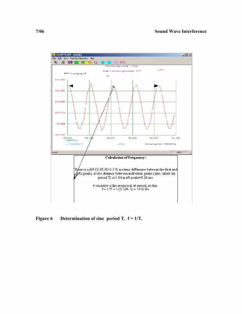
Figure 6 Determination of sine period T. f = 1/T.
7/06 Sound Wave Interference
B. Spatial Interference I A simple geometry
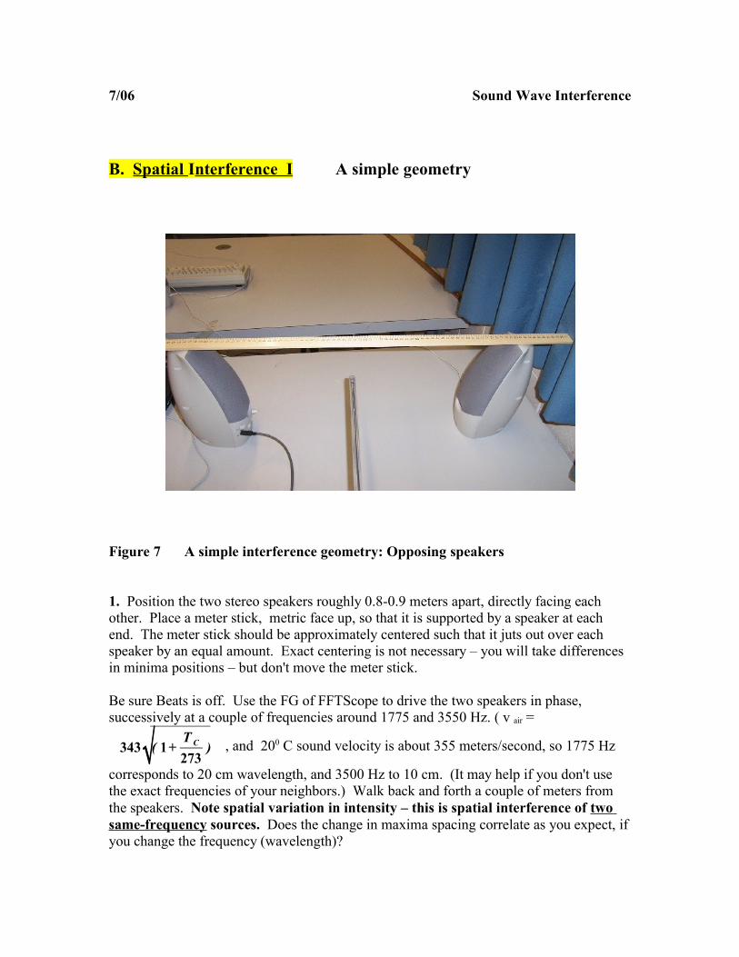
Figure 7 A simple interference geometry: Opposing speakers
1. Position the two stereo speakers roughly 0.8-0.9 meters apart, directly facing each other. Place a meter stick, metric face up, so that it is supported by a speaker at each end. The meter stick should be approximately centered such that it juts out over each speaker by an equal amount. Exact centering is not necessary – you will take differences in minima positions – but don't move the meter stick.
Be sure Beats is off. Use the FG of FFTScope to drive the two speakers in phase, successively at a couple of frequencies around 1775 and 3550 Hz. ( v air =
343( 1+T C
273) , and 200 C sound velocity is about 355 meters/second, so 1775 Hz
corresponds to 20 cm wavelength, and 3500 Hz to 10 cm. (It may help if you don't use the exact frequencies of your neighbors.) Walk back and forth a couple of meters from the speakers. Note spatial variation in intensity – this is spatial interference of two same-frequency sources. Does the change in maxima spacing correlate as you expect, if you change the frequency (wavelength)?

7/06 Sound Wave Interference
2. Run the small microphone at the end of the white “wand” along the stick and find nodes with the FFT spectrum analyzer. (Nodes may be easier to identify than antinodes. Auto scale may give you a visual peak stuck at max; the other scaling may be preferable. Your frequency peak amplitude should not be affected by your neighbor's frequency if the f's differ by 100 Hz or more.- coordinate).
If the mike is moved a half wave length, the distance from one speaker shortens by λ/2, and that from the otgher speaker lengthens by λ/2, so the net change in path difference is a full wavelength λ. Therefore the distances between successive nodes or antinodes is a half wavelength.
Record the positions of nodes (or of antinodes) and average the successive differences. Compare with the predicted wavelength v/f.
C. Phase Matters
Open one FFTScope, but leave the Function Generator silent. Open Interference.exe and set to 3550 Hz (10 cm) with phase = 0. Move your ear along the edge of the table in front of the parallel speakers. You should hear a central maximum, with minima on either side. Repeat, using the FFT display mode of FFTScope.
Now switch the Interference.exe phase to 180 and repeat. You should find a central mimnimum, with a maximum on either side. The entire pattern of maxima and minima is interchanged.
1800 phase shift is equivalent to an extra half-wavelength in the path length from one speaker.
D. Spatial Interference II
7/06 Sound Wave Interference
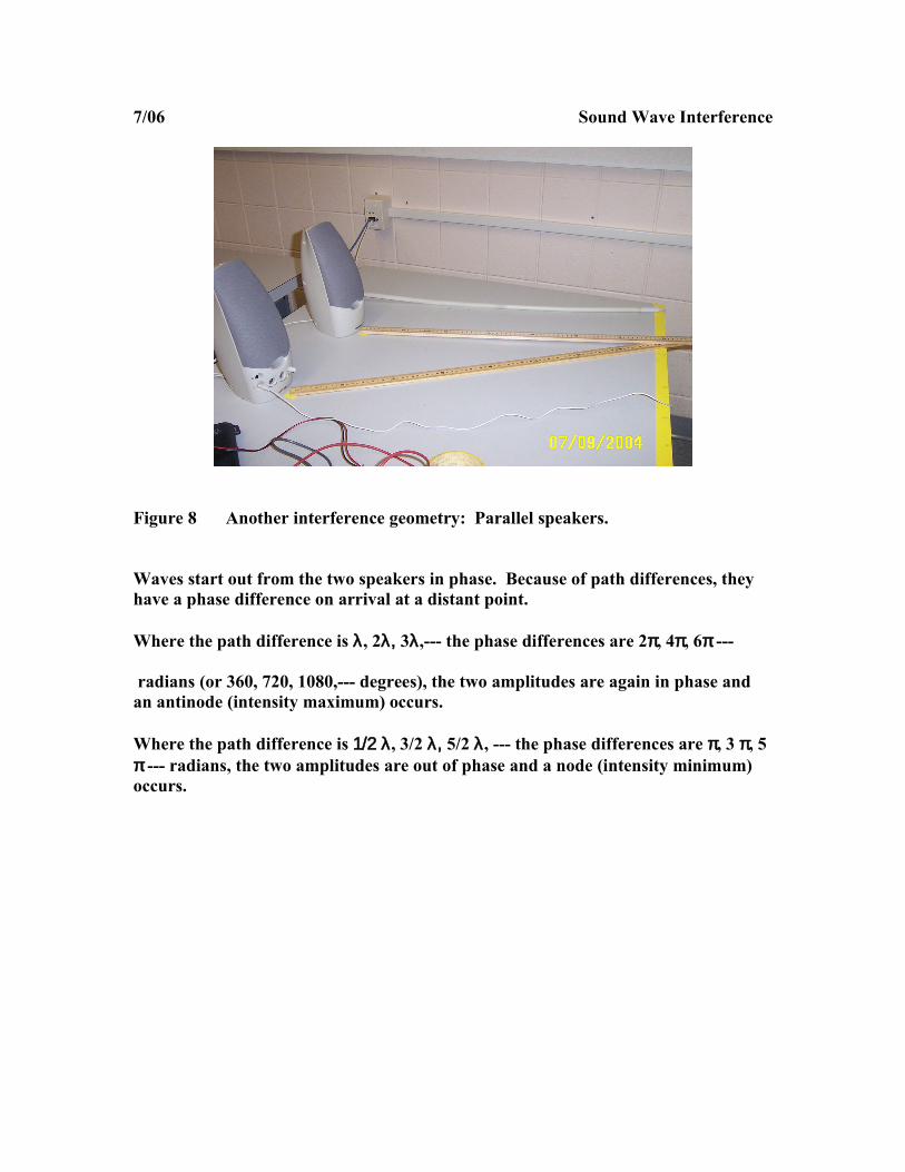
Figure 8 Another interference geometry: Parallel speakers.
Waves start out from the two speakers in phase. Because of path differences, they have a phase difference on arrival at a distant point.
Where the path difference is λ, 2λ, 3λ,--- the phase differences are 2π, 4π, 6π ---
radians (or 360, 720, 1080,--- degrees), the two amplitudes are again in phase and an antinode (intensity maximum) occurs.
Where the path difference is 1/2 λ, 3/2 λ, 5/2 λ, --- the phase differences are π, 3 π, 5 π --- radians, the two amplitudes are out of phase and a node (intensity minimum) occurs.

7/06 Sound Wave Interference
Figure 9 Refer to Figure 8. Calculated wave path differences along a line (Y) parallel at distance D = 60 cm to two sinusoidally driven speakers, separated by distance d = 30 cm. The violet straight line represents the d sin(θ) approximation. The blue line represents the actual path difference (r2-r1), (plus extra equivalent path produced by any non-zero speaker relative phase).
Crossings of integer m values by the prediction curves give the predicted y values where the net path difference (including extra path equivalent to non-zero speaker phase relation) is an integer number of wavelengths, i.e., locations of maxima.
Crossings of half-integer m values by the prediction curves give the predicted y values where the net path difference (including extra path equivalent to non-zero speaker phase relation) is a half-integer number of wavelengths, i.e., locations of minima.
For the calculation, the speaker separation was d = 30 cm, the speaker setback D from the observation line (y) was 60 cm, the wavelength λ = 10 cm (3500 Hertz) and the phase shift equivalent-extra-path was zero.

7/06 Sound Wave Interference
Figure 10 d =30, D = 60, λ= 10 centimeters.
Upper curve: + 5 cm equivalent (half-wave) extra path (+5/10 = +1800/3600; λ = 10 cm).Middle curve: 0 cm equivalent extra path (00 phase shift).Lower curve: -5 cm equivalent extra path or -1800 phase shift between speakers.
Note that the upper and lower curves predict minima at y = 0, whereas the middle curve (zero phase shift), predicts a maximum. The upper and lower curves predict an interchange of maxima and minima with the middle curve. The only difference in the upper and lower predictions is in the m labeling. The patterns are identical.
7/06 Sound Wave Interference
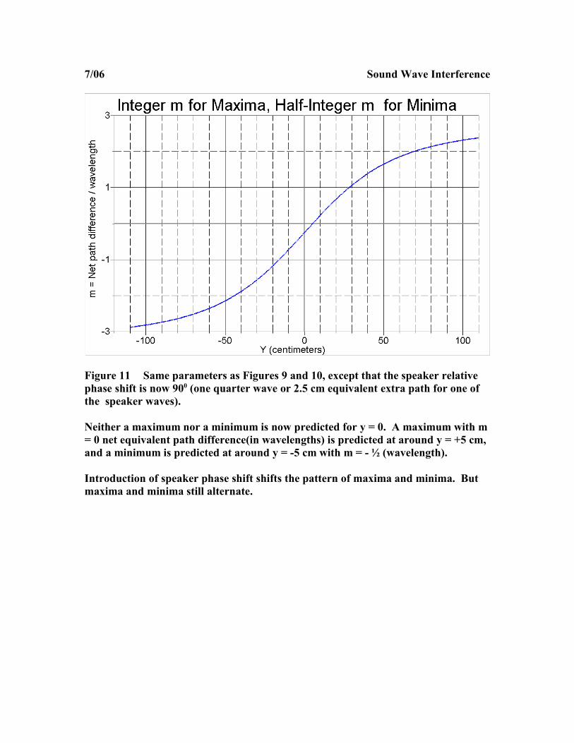
Figure 11 Same parameters as Figures 9 and 10, except that the speaker relative phase shift is now 900 (one quarter wave or 2.5 cm equivalent extra path for one of the speaker waves).
Neither a maximum nor a minimum is now predicted for y = 0. A maximum with m = 0 net equivalent path difference(in wavelengths) is predicted at around y = +5 cm, and a minimum is predicted at around y = -5 cm with m = - ½ (wavelength).
Introduction of speaker phase shift shifts the pattern of maxima and minima. But maxima and minima still alternate.
7/06 Sound Wave Interference
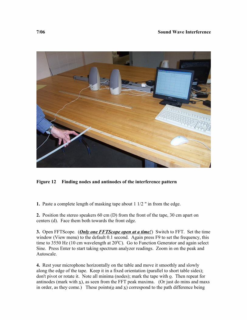
Figure 12 Finding nodes and antinodes of the interference pattern
1. Paste a complete length of masking tape about 1 1/2 " in from the edge.
2. Position the stereo speakers 60 cm (D) from the front of the tape, 30 cm apart on centers (d). Face them both towards the front edge.
3. Open FFTScope. (Only one FFTScope open at a time!) Switch to FFT. Set the time window (View menu) to the default 0.1 second. Again press F9 to set the frequency, this time to 3550 Hz (10 cm wavelength at 200C). Go to Function Generator and again select Sine. Press Enter to start taking spectrum analyzer readings. Zoom in on the peak and Autoscale.
4. Rest your microphone horizontally on the table and move it smoothly and slowly along the edge of the tape. Keep it in a fixed orientation (parallel to short table sides); don't pivot or rotate it. Note all minima (nodes); mark the tape with o. Then repeat for antinodes (mark with x), as seen from the FFT peak maxima. (Or just do mins and maxs in order, as they come.) These points(o and x) correspond to the path difference being
7/06 Sound Wave Interference
half/integral or integral number of full wavelengths. Find the two nodes to right and left of the speaker center. Draw the center line half way between.
Label all o's to the right: +1/2, +3/2, etc. Label all o's to the left: -1/2, -3/2, etc.Label the central x: 0. Label all x's to the right: +1, +2, etc. Label all x-s to the left: -1, -2, etc.
Measuring from your center line (not from the m = 0 cxemtral maximum), record on the tape all y distances to nodes and antinodes, + to right, - to left. Enter the (y,m) values (with signs) in the data table. Then enter the (y,m) pairs in the Graphical Analysis data table for 10 cm wavelength, nodes in the "mins" column, antinodes in the "maxs" column. Enter at the closest value in the "y" data column. Examine the corresponding plot, which shows two theoretical curves of relative phase, one for (r2-r1)/λ and one for d sin(θ)/λ.
Paste a fresh tape and repeat for 7100 Hz (5 cm wavelength at 200C).
[Note: We are considering only phase differences, ignoring any effect on the position of maxima and minima of intensity differences due to difference in distance from the two speakers.]
Print your curves for 5 and 10 centimeter waves.
A Review of Alternative Wave Descriptions
Waveform description: Time and space specification:
A harmonic wave is a periodic oscillation of sinusoidal form whose shape does not change.
A static sinusoid has the form y( x )= sin ( x ) . To make this wave move, let us add a time dependence:
y( x , t )= y0 sin ( x - v t ) (a wave moving to the right (+x) direction with speed v)
A more general expression which specifies parameters such as the maximum displacement of the wave (amplitude), frequency and wavelength is:
7/06 Sound Wave Interference
y( x , t )= y0 sin ( kx - t )
where y0 is the amplitude, k =2
is the “wave number” in radians per meter and
= 2 f =2T
is the “angular frequency” of the wave in radians per second.
At time t=0, the wave at fixed observation point x is:
y( x ,0 )= y0sin ( kx )
One whole period T later (the time it takes for a wave to traverse a fixed point), the wave is:
y( x ,T )= y0sin( kx - t )
However, since = 2 f and f = 1T , T = 2 and the equation reads
y( x ,T )= y0sin( kx - 2 )= y0sin( kx ) since sine repeats every 2π .
The wave value at fixed x is the same one period later at time t=T as it was at time t=0.
Similarly, the wave value at fixed t is the same as that one wavelength away.
Frequency composition: Amplitude and phase specification:
Fourier's theorem allows any periodic function to be described as the sum of a series of sinusoidal functions:
f ( t )= An sin ( n0 t ) where 0 is the fundamental (lowest) angular frequency and the An are the Fourier coefficients).
For example, a square wave can be represented by the above equation with
7/06 Sound Wave Interference
An = - 4n
(−1 )n+1
2
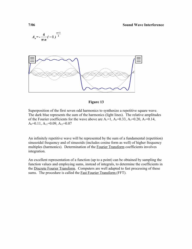
Figure 13
Superposition of the first seven odd harmonics to synthesize a repetitive square wave. The dark blue represents the sum of the harmonics (light lines). The relative amplitudes of the Fourier coefficients for the wave above are A1=1, A3=0.33, A5=0.20, A7=0.14, A9=0.11, A11=0.09, A13=0.07
An infinitely repetitive wave will be represented by the sum of a fundamental (repetition) sinusoidal frequency and of sinusoids (includes cosine form as well) of higher frequency multiples (harmonics). Determination of the Fourier Transform coefficients involves integration.
An excellent representation of a function (up to a point) can be obtained by sampling the function values and employing sums, instead of integrals, to determine the coefficients in the Discrete Fourier Transform. Computers are well adapted to fast processing of these sums. The procedure is called the Fast Fourier Transform (FFT).