Source localization in an ocean waveguide using supervisedmachine learning

Haiqiang Niu,a) Emma Reeves, and Peter GerstoftScripps Institution of Oceanography, University of California San Diego, La Jolla, California 92093-0238,USA

(Received 9 December 2016; revised 18 June 2017; accepted 8 August 2017; published online 1September 2017)

Source localization in ocean acoustics is posed as a machine learning problem in which data-drivenmethods learn source ranges directly from observed acoustic data. The pressure received by avertical linear array is preprocessed by constructing a normalized sample covariance matrix andused as the input for three machine learning methods: feed-forward neural networks (FNN), supportvector machines (SVM), and random forests (RF). The range estimation problem is solved both asa classification problem and as a regression problem by these three machine learning algorithms.The results of range estimation for the Noise09 experiment are compared for FNN, SVM, RF,and conventional matched-field processing and demonstrate the potential of machine learning forunderwater source localization. VC 2017 Acoustical Society of America.[http://dx.doi.org/10.1121/1.5000165]

[SED] Pages: 1176–1188

I. INTRODUCTION

Machine learning is a promising method for locatingocean sources because of its ability to learn features fromdata, without requiring sound propagation modeling. It canbe used for unknown environments.

Acoustic source localization in ocean waveguides isoften solved with matched-field processing (MFP).1–13

Despite the success of MFP, it is limited in some practicalapplications due to its sensitivity to the mismatch betweenmodel-generated replica fields and measurements. MFPgives reasonable predictions only if the ocean environmentcan be accurately modeled. Unfortunately, this is difficultbecause the realistic ocean environment is complicated andunstable.

An alternative approach to the source localization prob-lem is to find features directly from data.14–17 Interest inmachine learning techniques has been revived thanks toincreased computational resources as well as their ability tolearn nonlinear relationships. A notable recent example inocean acoustics is the application of nonlinear regression tosource localization.18 Other machine learning methods haveobtained remarkable results when applied to areas such asspeech recognition,19 image processing,20 natural languageprocessing,21 and seismology.22–25 Most underwater acous-tics research in machine learning is based on 1990s neuralnetworks. Previous research has applied neutral networks todetermine the source location in a homogeneous medium,26

simulated range and depth discrimination using artificialneural networks in matched-field processing,27 estimatedocean-sediment properties using radial basis functions inregression and neural networks,28,29 applied artificial neural

networks to estimation of geoacoustic model parameters,30,31

classification of seafloor32 and whale sounds.33

This paper explores the use of current machine learningmethods for source range localization. The feed-forwardneural network (FNN), support vector machine (SVM), andrandom forest (RF) methods are investigated. There are sev-eral main differences between our work and previous studiesof source localization and inversion:18,26–33

(1) Acoustic observations are used to train the machine learningmodels instead of using model-generated fields.26,27,29–31

(2) For input data, normalized sample covariance matrices,including amplitude and phase information, are used.Other alternatives include the complex pressure,18 phasedifference,26 eigenvalues,27 amplitude of the pressurefield,29 transmission loss,30,31 angular dependence ofbackscatter,32 or features extracted from spectrograms.33

This preprocessing procedure is known as feature extrac-tion in machine learning.

(3) Under machine learning framework, source localizationcan be solved as a classification or a regression problem.This work focuses on classification in addition to theregression approach used in previous studies.18,26,28–31

(4) Well-developed machine learning libraries are used.Presently, there are numerous efficient open sourcemachine learning libraries available, includingTensorFlow,34 Scikit-learn,35 Theano,36 Caffe,37 andTorch,38 all of which solve typical machine learning taskswith comparable efficiency. Here, TensorFlow is used toimplement FNN because of its simple architecture andwide user base. Scikit-learn is used to implement SVM andRF as they are not included in the current TensorFlow ver-sion. Compared to older neural network implementations,Tensorflow includes improved optimization algorithms39

with better convergence, more robust model with dropout40

technique and high computational efficiency.

a)Also at: State Key Laboratory of Acoustics, Institute of Acoustics, ChineseAcademy of Sciences, Beijing 100190, People’s Republic of China.Electronic mail: hniu@ucsd.edu

1176 J. Acoust. Soc. Am. 142 (3), September 2017 VC 2017 Acoustical Society of America0001-4966/2017/142(3)/1176/13/$30.00

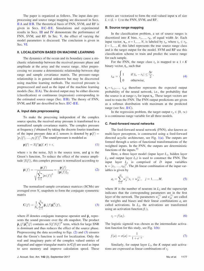
The paper is organized as follows. The input data pre-processing and source range mapping are discussed in Secs.II A and II B. The theoretical basis of FNN, SVM, and RF isgiven in Secs. II C–II E. Simulations and experimentalresults in Secs. III and IV demonstrate the performance ofFNN, SVM, and RF. In Sec. V, the effect of varying themodel parameters is discussed. The conclusion is given inSec. VI.

II. LOCALIZATION BASED ON MACHINE LEARNING

The dynamics of the ocean and its boundary cause a sto-chastic relationship between the received pressure phase andamplitude at the array and the source range. After prepro-cessing we assume a deterministic relationship between shiprange and sample covariance matrix. The pressure–rangerelationship is in general unknown but may be discoveredusing machine learning methods. The received pressure ispreprocessed and used as the input of the machine learningmodels (Sec. II A). The desired output may be either discrete(classification) or continuous (regression) corresponding tothe estimated source range (Sec. II B). The theory of FNN,SVM, and RF are described in Secs. II C–II E.

A. Input data preprocessing

To make the processing independent of the complexsource spectra, the received array pressure is transformed to anormalized sample covariance matrix. The complex pressureat frequency f obtained by taking the discrete fourier transformof the input pressure data at L sensors is denoted by pðf Þ ¼½p1ðf Þ;…; pLðf Þ%T . The sound pressure is modeled as

pðf Þ ¼ Sðf Þgðf ; rÞ þ !; (1)

where ! is the noise, S(f) is the source term, and g is theGreen’s function. To reduce the effect of the source ampli-tude jSðf Þj, this complex pressure is normalized according to

~p fð Þ ¼p fð Þffiffiffiffiffiffiffiffiffiffiffiffiffiffiffiffiffiffiffiffiffiffiffi

XL

l¼1

jpl fð Þj2s ¼ p fð Þ

kp fð Þk2

: (2)

The normalized sample covariance matrices (SCMs) areaveraged over Ns snapshots to form the conjugate symmetricmatrix

C fð Þ ¼1

Ns

XNs

s¼1

~ps fð Þ~pHs fð Þ; (3)

where H denotes conjugate transpose operator and ~ps repre-sents the sound pressure over the sth snapshot. The product~psðf Þ~pH

s ðf Þ contains an Sðf ÞSðf ÞH term, which for large SNRis dominant and thus reduces the effect of the source phase.Preprocessing the data according to Eqs. (2) and (3) ensuresthat the Green’s function is used for localization. Only thereal and imaginary parts of the complex valued entries ofdiagonal and upper triangular matrix in C(f) are used as inputto save memory and improve calculation speed. These

entries are vectorized to form the real-valued input x of sizeL' (L þ 1) to the FNN, SVM, and RF.

B. Source range mapping

In the classification problem, a set of source ranges isdiscretized into K bins, r1,…, rK, of equal width Dr. Eachinput vector, xn, n¼ 1,…, N, is labeled by tn, where tn 2 rk,k¼ 1,…, K; this label represents the true source range classand is the target output for the model. SVM and RF use thisclassification scheme to train and predict the source rangefor each sample.

For the FNN, the range class tn is mapped to a 1'Kbinary vector, tn, such that

tnk ¼1 if jtn ( rkj )

Dr

2;

0 otherwise;

8<

: (4)

tn¼ tn,1,…, tn,K therefore represents the expected outputprobability of the neural network, i.e., the probability thatthe source is at range rk for input xn. These target vectors areused to train the FNN. The FNN output predictions are givenas a softmax distribution with maximum at the predictedrange (see Sec. II C).

In the regression problem, the target output rn 2 [0, 1)is a continuous range variable for all three models.

C. Feed-forward neural networks

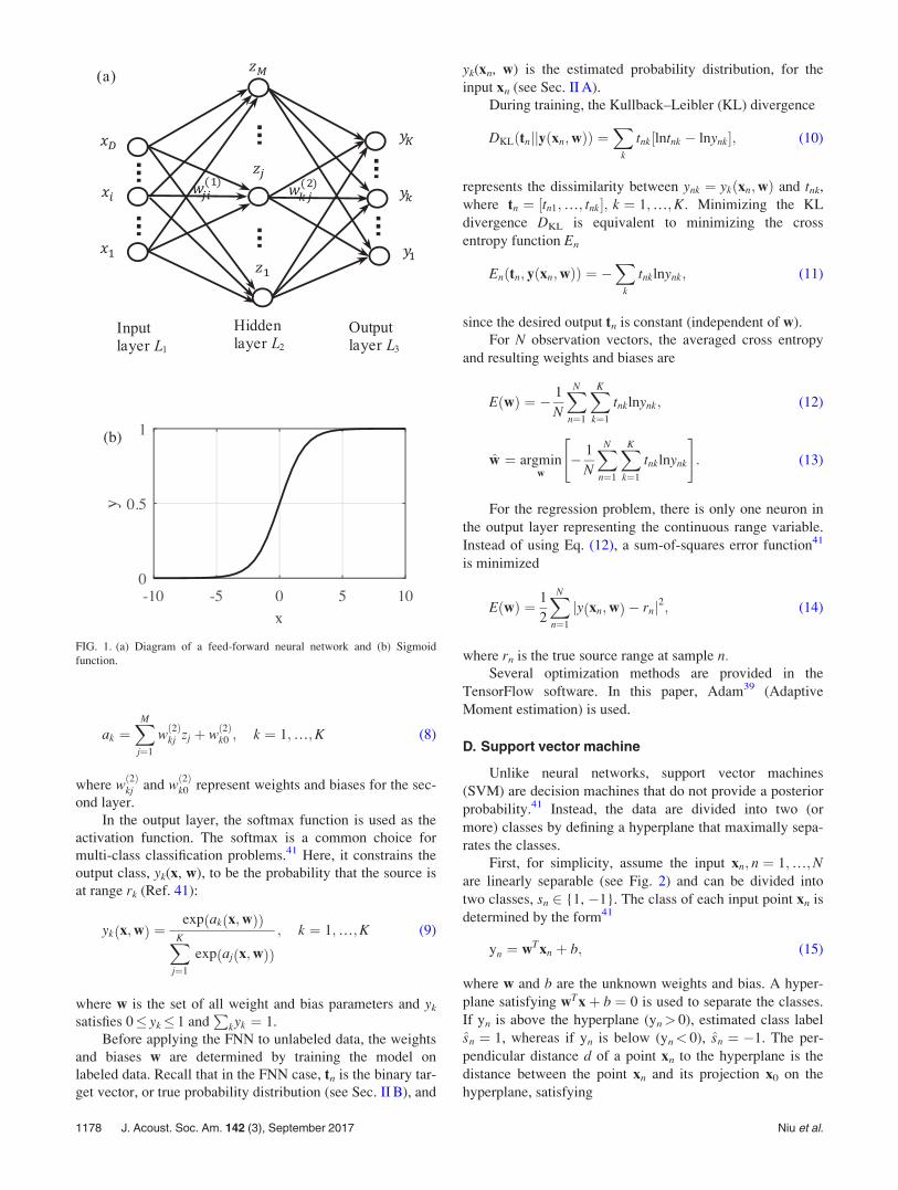
The feed-forward neural network (FNN), also known asmulti-layer perceptron, is constructed using a feed-forwarddirected acyclic architecture, see Fig. 1(a). The outputs areformed through a series of functional transformations of theweighted inputs. In the FNN, the outputs are deterministicfunctions of the inputs.41

Here, a three layer model (input layer L1, hidden layerL2 and output layer L3) is used to construct the FNN. Theinput layer L1 is comprised of D input variablesx ¼ ½x1;…; xD%T . The jth linear combination of the input var-iables is given by

aj ¼XD

i¼1

wð1Þji xi þ wð1Þj0 ; j ¼ 1;…;M; (5)

where M is the number of neurons in L2 and the superscriptindicates that the corresponding parameters are in the firstlayer of the network. The parameters wð1Þji and wð1Þj0 are calledthe weights and biases and their linear combinations aj arecalled activations. In L2, the activations are transformedusing an activation function f(*),

zj ¼ f ðajÞ: (6)

The logistic sigmoid was chosen as the intermediate activa-tion function for this study, see Fig. 1(b):

f að Þ ¼ r að Þ ¼1

1þ e(a: (7)

Similarly, for output layer L3, the K output unit activa-tions are expressed as linear combinations of zj

J. Acoust. Soc. Am. 142 (3), September 2017 Niu et al. 1177

ak ¼XM

j¼1

wð2Þkj zj þ wð2Þk0 ; k ¼ 1;…;K (8)

where wð2Þkj and wð2Þk0 represent weights and biases for the sec-ond layer.

In the output layer, the softmax function is used as theactivation function. The softmax is a common choice formulti-class classification problems.41 Here, it constrains theoutput class, yk(x, w), to be the probability that the source isat range rk (Ref. 41):

yk x;wð Þ ¼exp ak x;wð Þð Þ

XK

j¼1

exp aj x;wð Þð Þ

; k ¼ 1;…;K (9)

where w is the set of all weight and bias parameters and yk

satisfies 0) yk) 1 andP

kyk ¼ 1.Before applying the FNN to unlabeled data, the weights

and biases w are determined by training the model onlabeled data. Recall that in the FNN case, tn is the binary tar-get vector, or true probability distribution (see Sec. II B), and

yk(xn, w) is the estimated probability distribution, for theinput xn (see Sec. II A).

During training, the Kullback–Leibler (KL) divergence

DKLðtnjjyðxn;wÞÞ ¼X

k

tnk lntnk ( lnynk½ %; (10)

represents the dissimilarity between ynk ¼ ykðxn;wÞ and tnk,where tn ¼ ½tn1;…; tnk%; k ¼ 1;…;K. Minimizing the KLdivergence DKL is equivalent to minimizing the crossentropy function En

Enðtn; yðxn;wÞÞ ¼ (X

k

tnklnynk; (11)

since the desired output tn is constant (independent of w).For N observation vectors, the averaged cross entropy

and resulting weights and biases are

E wð Þ ¼ (1

N

XN

n¼1

XK

k¼1

tnklnynk; (12)

w ¼ argminw

( 1

N

XN

n¼1

XK

k¼1

tnklnynk

" #

: (13)

For the regression problem, there is only one neuron inthe output layer representing the continuous range variable.Instead of using Eq. (12), a sum-of-squares error function41

is minimized

E wð Þ ¼1

2

XN

n¼1

jy xn;wð Þ ( rnj2; (14)

where rn is the true source range at sample n.Several optimization methods are provided in the

TensorFlow software. In this paper, Adam39 (AdaptiveMoment estimation) is used.

D. Support vector machine

Unlike neural networks, support vector machines(SVM) are decision machines that do not provide a posteriorprobability.41 Instead, the data are divided into two (ormore) classes by defining a hyperplane that maximally sepa-rates the classes.

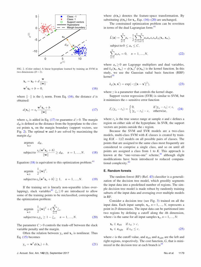
First, for simplicity, assume the input xn; n ¼ 1;…;Nare linearly separable (see Fig. 2) and can be divided intotwo classes, sn 2 {1, (1}. The class of each input point xn isdetermined by the form41

yn ¼ wTxn þ b; (15)

where w and b are the unknown weights and bias. A hyper-plane satisfying wTxþ b ¼ 0 is used to separate the classes.If yn is above the hyperplane (yn> 0), estimated class labelsn ¼ 1, whereas if yn is below (yn< 0), sn ¼ (1. The per-pendicular distance d of a point xn to the hyperplane is thedistance between the point xn and its projection x0 on thehyperplane, satisfying

FIG. 1. (a) Diagram of a feed-forward neural network and (b) Sigmoidfunction.

1178 J. Acoust. Soc. Am. 142 (3), September 2017 Niu et al.

xn ¼ x0 þ dw

jjwjj;

wTx0 þ b ¼ 0; (16)

where k * k is the l2 norm. From Eq. (16), the distance d isobtained:

d xnð Þ ¼ snwTxn þ b

kwk; (17)

where sn is added in Eq. (17) to guarantee d> 0. The margindM is defined as the distance from the hyperplane to the clos-est points xs on the margin boundary (support vectors, seeFig. 2). The optimal w and b are solved by maximizing themargin dM:

argmaxw;b

dM;

subject tosn wTxn þ bð Þkwk

+ dM; n ¼ 1;…;N: (18)

Equation (18) is equivalent to this optimization problem:41

argminw;b

1

2kwk2;

subject to sn wTxn þ b" #

+ 1; n ¼ 1;…;N: (19)

If the training set is linearly non-separable (class over-lapping), slack variables41 nn+ 0 are introduced to allowsome of the training points to be miclassified, correspondingthe optimization problem:

argminw;b

1

2kwk2 þ C

XN

n¼1

nn;

subject to snyn + 1( nn; n ¼ 1;…;N: (20)

The parameter C> 0 controls the trade-off between the slackvariable penalty and the margin.

Often the relation between yn and xn is nonlinear. ThusEq. (15) becomes

yn ¼ wT/ðxnÞ þ b; (21)

where /(xn) denotes the feature-space transformation. Bysubstituting /(xn) for xn, Eqs. (16)–(20) are unchanged.

The constrained optimization problem can be rewrittenin terms of the dual Lagrangian form:41

~L að Þ ¼XN

n¼1

an (1

2

XN

n¼1

XN

m¼1

anamsnsmk/ xn; xmð Þ;

subject to 0 ) an ) C;

XN

n¼1

ansn ¼ 0; n ¼ 1;…;N; (22)

where an+ 0 are Lagrange multipliers and dual variables,and k/ðxn; xmÞ ¼ /ðxnÞT/ðxmÞ is the kernel function. In thisstudy, we use the Gaussian radial basis function (RBF)kernel35

k/ðx; x0Þ ¼ expð(ckx( x0k2Þ; (23)

where c is a parameter that controls the kernel shape.Support vector regression (SVR) is similar to SVM, but

it minimizes the !–sensitive error function

E!ðyn ( rnÞ ¼0; if jyn ( rnj < !;jyn ( rnj( !; otherwise;

$(24)

where rn is the true source range at sample n and ! defines aregion on either side of the hyperplane. In SVR, the supportvectors are points outside the ! region.

Because the SVM and SVR models are a two-classmodels, multi-class SVM with K classes is created by train-ing K(K – 1)/2 models on all possible pairs of classes. Thepoints that are assigned to the same class most frequently areconsidered to comprise a single class, and so on until allpoints are assigned a class from 1 to K. This approach isknown at the “one-versus-one” scheme,41 although slightmodifications have been introduced to reduced computa-tional complexity.42

E. Random forests

The random forest (RF) (Ref. 43) classifier is a generali-zation of the decision tree model, which greedily segmentsthe input data into a predefined number of regions. The sim-ple decision tree model is made robust by randomly trainingsubsets of the input data and averaging over multiple modelsin RF.

Consider a decision tree (see Fig. 3) trained on all theinput data. Each input sample, xn, n¼ 1,…, N, represents apoint in D dimensions. The input data can be partitioned intotwo regions by defining a cutoff along the ith dimension,where i is the same for all input samples xn, n¼ 1,…, N:

xn 2 xleft if xni > c;

xn 2 xright if xni ) c; (25)

where c is the cutoff value, and xleft and xright are the left andright regions, respectively. The cost function, G, that is mini-mized in the decision tree at each branch is35

FIG. 2. (Color online) A linear hyperplane learned by training an SVM intwo dimensions (D¼ 2).

J. Acoust. Soc. Am. 142 (3), September 2017 Niu et al. 1179

c, ¼ argminc

G cð Þ;

G cð Þ ¼nleft

NH xleftð Þ þ

nright

NH xrightð Þ; (26)

where nleft and nright are the numbers of points in the regionsxleft and xright. H(*) is an impurity function chosen based onthe problem.

For the classification problem, the Gini index35 is cho-sen as the impurity function

H xmð Þ ¼1

nm

X

xn2xm

I tn; ‘mð Þ 1( 1

nmI tn; ‘mð Þ

% &; (27)

where nm is the number of points in region xm and ‘m repre-sents the assigned label for each region, corresponding to themost common class in the region:35

‘m ¼ argmaxrk

X

xn2xm

Iðtn; rkÞ: (28)

In Eq. (28), rk, k¼ 1,…, K are the source range classes and tnis the label of point xn in region m, and

Iðtn; rkÞ ¼1 if tn ¼ rk;0 otherwise:

$(29)

The remaining regions are partitioned iteratively untilregions x1;…; xM are defined. In this paper, the number of

regions, M, is determined by the minimum number of pointsallowed in a region. A diagram of the decision tree classifieris shown in Fig. 3. The samples are partitioned into M¼ 3regions with the cutoff values 1.9 and 4.6.

For RF regression, there are two differences from classi-fication: the estimated class for each region is defined as themean of the true class for all points in the region, and themean squared error is used as the impurity function

‘m ¼1

nm

X

xn2xm

rn;

H xmð Þ ¼X

xn2xm

‘m ( rnð Þ2; (30)

where rn is source range at sample n.As the decision tree model may overfit the data, statisti-

cal bootstrap and bagging are used to create a more robustmodel, a random forest.44 In a given draw, the input data,xi; i ¼ 1;…;Q, is selected uniformly at random from the fulltraining set, where Q)N. B such draws are conducted withreplacement and a new decision tree is fitted to each subsetof data. Each point, xn, is assigned to its most frequent classamong all draws:

fbagðxnÞ ¼ argmax

tn

XB

b¼1

Iðf tree;bðxnÞ; tnÞ; (31)

where ftree;bðxiÞ is the class of xi for the bth tree.

F. Performance metric

To quantify the prediction performance of the rangeestimation methods, the mean absolute percentage error(MAPE) over N samples is defined as

EMAPE ¼100

N

XN

i¼1

Rpi ( Rgi

Rgi

''''

''''; (32)

where Rpi and Rgi are the predicted range and the groundtruth range, respectively. MAPE is preferred as an error mea-sure because it accounts for the magnitude of error in faultyrange estimates as well as the frequency of correct estimates.MAPE is known to be an asymmetric error measure45 but isadequate for the small range of outputs considered.

G. Source localization algorithm

The localization problem solved by machine learning isimplemented as follows:

(1) Data preprocessing. The recorded pressure signals areFourier transformed and Ns snapshots form the SCMfrom which the input x is formed.

(2) Division of preprocessed data into training and test datasets. For the training data, the labels are prepared basedon different machine learning algorithms.

(3) Training the machine learning models. X ¼ ½x1…xN% areused as the training input and the corresponding labels asthe desired output.

FIG. 3. (Color online) Decision tree classifier and corresponding rectangularregions shown for two–dimensional data with K¼ 2 classes (D¼ 2, M¼ 3)and 1000 training points.

1180 J. Acoust. Soc. Am. 142 (3), September 2017 Niu et al.

(4) Prediction on unlabeled data. The model parameterstrained in step 3 are used to predict the source range fortest data. The resulting output is mapped back to range,and the prediction error is reported by the mean absolutepercentage error.

III. SIMULATIONS

In this section, the performance of machine learning onsimulated data are discussed. For brevity, only the FNN clas-sifier is examined here, although the conclusions apply toSVM and RF. Further discussion of SVM and RF perfor-mance is included in Secs. IV and V.

A. Environmental model and source-receiverconfiguration

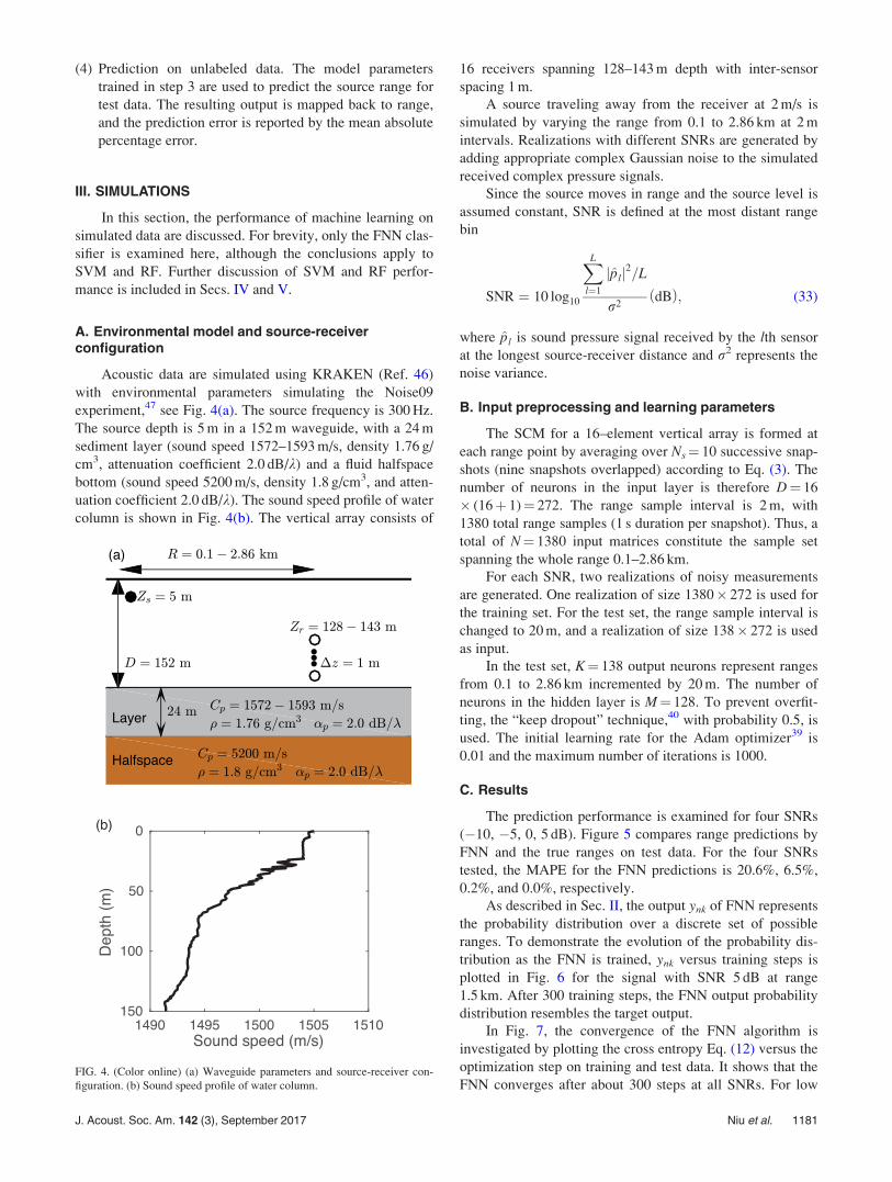
Acoustic data are simulated using KRAKEN (Ref. 46)with environmental parameters simulating the Noise09experiment,47 see Fig. 4(a). The source frequency is 300 Hz.The source depth is 5 m in a 152 m waveguide, with a 24 msediment layer (sound speed 1572–1593 m/s, density 1.76 g/cm3, attenuation coefficient 2.0 dB/k) and a fluid halfspacebottom (sound speed 5200 m/s, density 1.8 g/cm3, and atten-uation coefficient 2.0 dB/k). The sound speed profile of watercolumn is shown in Fig. 4(b). The vertical array consists of

16 receivers spanning 128–143 m depth with inter-sensorspacing 1 m.

A source traveling away from the receiver at 2 m/s issimulated by varying the range from 0.1 to 2.86 km at 2 mintervals. Realizations with different SNRs are generated byadding appropriate complex Gaussian noise to the simulatedreceived complex pressure signals.

Since the source moves in range and the source level isassumed constant, SNR is defined at the most distant rangebin

SNR ¼ 10 log10

XL

l¼1

jplj2=L

r2dBð Þ; (33)

where pl is sound pressure signal received by the lth sensorat the longest source-receiver distance and r2 represents thenoise variance.

B. Input preprocessing and learning parameters

The SCM for a 16–element vertical array is formed ateach range point by averaging over Ns¼ 10 successive snap-shots (nine snapshots overlapped) according to Eq. (3). Thenumber of neurons in the input layer is therefore D¼ 16' (16þ 1)¼ 272. The range sample interval is 2 m, with1380 total range samples (1 s duration per snapshot). Thus, atotal of N¼ 1380 input matrices constitute the sample setspanning the whole range 0.1–2.86 km.

For each SNR, two realizations of noisy measurementsare generated. One realization of size 1380' 272 is used forthe training set. For the test set, the range sample interval ischanged to 20 m, and a realization of size 138' 272 is usedas input.

In the test set, K¼ 138 output neurons represent rangesfrom 0.1 to 2.86 km incremented by 20 m. The number ofneurons in the hidden layer is M¼ 128. To prevent overfit-ting, the “keep dropout” technique,40 with probability 0.5, isused. The initial learning rate for the Adam optimizer39 is0.01 and the maximum number of iterations is 1000.

C. Results

The prediction performance is examined for four SNRs((10, (5, 0, 5 dB). Figure 5 compares range predictions byFNN and the true ranges on test data. For the four SNRstested, the MAPE for the FNN predictions is 20.6%, 6.5%,0.2%, and 0.0%, respectively.

As described in Sec. II, the output ynk of FNN representsthe probability distribution over a discrete set of possibleranges. To demonstrate the evolution of the probability dis-tribution as the FNN is trained, ynk versus training steps isplotted in Fig. 6 for the signal with SNR 5 dB at range1.5 km. After 300 training steps, the FNN output probabilitydistribution resembles the target output.

In Fig. 7, the convergence of the FNN algorithm isinvestigated by plotting the cross entropy Eq. (12) versus theoptimization step on training and test data. It shows that theFNN converges after about 300 steps at all SNRs. For low

FIG. 4. (Color online) (a) Waveguide parameters and source-receiver con-figuration. (b) Sound speed profile of water column.

J. Acoust. Soc. Am. 142 (3), September 2017 Niu et al. 1181

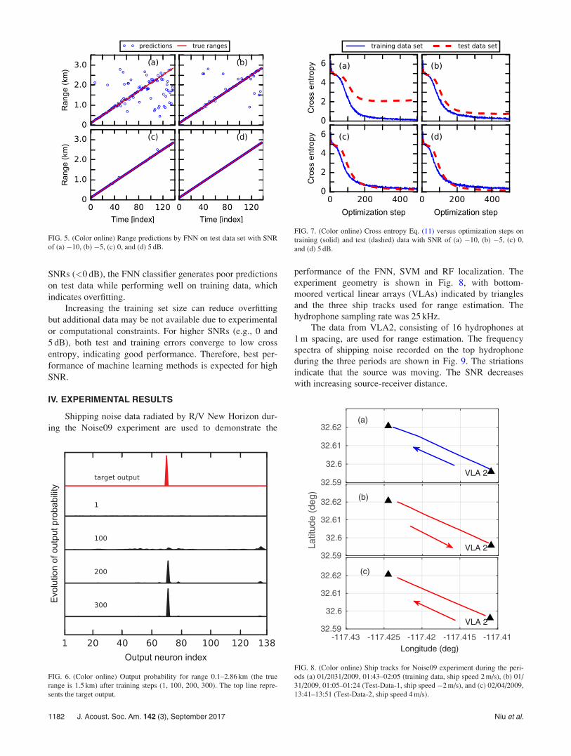
SNRs (<0 dB), the FNN classifier generates poor predictionson test data while performing well on training data, whichindicates overfitting.

Increasing the training set size can reduce overfittingbut additional data may be not available due to experimentalor computational constraints. For higher SNRs (e.g., 0 and5 dB), both test and training errors converge to low crossentropy, indicating good performance. Therefore, best per-formance of machine learning methods is expected for highSNR.

IV. EXPERIMENTAL RESULTS

Shipping noise data radiated by R/V New Horizon dur-ing the Noise09 experiment are used to demonstrate the

performance of the FNN, SVM and RF localization. Theexperiment geometry is shown in Fig. 8, with bottom-moored vertical linear arrays (VLAs) indicated by trianglesand the three ship tracks used for range estimation. Thehydrophone sampling rate was 25 kHz.

The data from VLA2, consisting of 16 hydrophones at1 m spacing, are used for range estimation. The frequencyspectra of shipping noise recorded on the top hydrophoneduring the three periods are shown in Fig. 9. The striationsindicate that the source was moving. The SNR decreaseswith increasing source-receiver distance.

FIG. 5. (Color online) Range predictions by FNN on test data set with SNRof (a) (10, (b) (5, (c) 0, and (d) 5 dB.

FIG. 6. (Color online) Output probability for range 0.1–2.86 km (the truerange is 1.5 km) after training steps (1, 100, 200, 300). The top line repre-sents the target output.

FIG. 7. (Color online) Cross entropy Eq. (11) versus optimization steps ontraining (solid) and test (dashed) data with SNR of (a) (10, (b) (5, (c) 0,and (d) 5 dB.

FIG. 8. (Color online) Ship tracks for Noise09 experiment during the peri-ods (a) 01/2031/2009, 01:43–02:05 (training data, ship speed 2 m/s), (b) 01/31/2009, 01:05–01:24 (Test-Data-1, ship speed (2 m/s), and (c) 02/04/2009,13:41–13:51 (Test-Data-2, ship speed 4 m/s).

1182 J. Acoust. Soc. Am. 142 (3), September 2017 Niu et al.

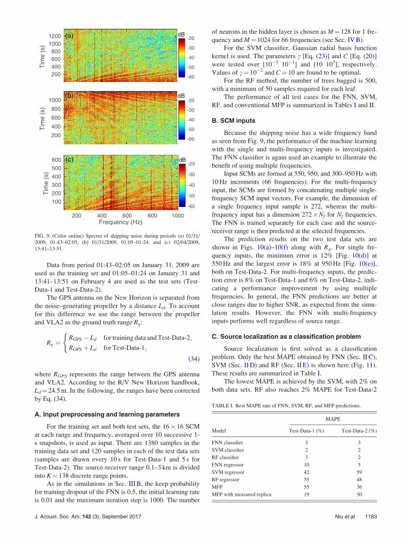
Data from period 01:43–02:05 on January 31, 2009 areused as the training set and 01:05–01:24 on January 31 and13:41–13:51 on February 4 are used as the test sets (Test-Data-1 and Test-Data-2).

The GPS antenna on the New Horizon is separated fromthe noise–generating propeller by a distance Ld. To accountfor this difference we use the range between the propellerand VLA2 as the ground truth range Rg:

Rg ¼RGPS ( Ld for training data and Test-Data-2;

RGPS þ Ld for Test-Data-1;

(

(34)

where RGPS represents the range between the GPS antennaand VLA2. According to the R/V New Horizon handbook,Ld¼ 24.5 m. In the following, the ranges have been correctedby Eq. (34).

A. Input preprocessing and learning parameters

For the training set and both test sets, the 16' 16 SCMat each range and frequency, averaged over 10 successive 1-s snapshots, is used as input. There are 1380 samples in thetraining data set and 120 samples in each of the test data sets(samples are drawn every 10 s for Test-Data-1 and 5 s forTest-Data-2). The source-receiver range 0.1–3 km is dividedinto K¼ 138 discrete range points.

As in the simulations in Sec. III B, the keep probabilityfor training dropout of the FNN is 0.5, the initial learning rateis 0.01 and the maximum iteration step is 1000. The number

of neurons in the hidden layer is chosen as M¼ 128 for 1 fre-quency and M¼ 1024 for 66 frequencies (see Sec. IV B).

For the SVM classifier, Gaussian radial basis functionkernel is used. The parameters c [Eq. (23)] and C [Eq. (20)]were tested over [10(3 10(1] and [10 103], respectively.Values of c¼ 10(2 and C¼ 10 are found to be optimal.

For the RF method, the number of trees bagged is 500,with a minimum of 50 samples required for each leaf.

The performance of all test cases for the FNN, SVM,RF, and conventional MFP is summarized in Tables I and II.

B. SCM inputs

Because the shipping noise has a wide frequency bandas seen from Fig. 9, the performance of the machine learningwith the single and multi-frequency inputs is investigated.The FNN classifier is again used an example to illustrate thebenefit of using multiple frequencies.

Input SCMs are formed at 550, 950, and 300–950 Hz with10 Hz increments (66 frequencies). For the multi-frequencyinput, the SCMs are formed by concatenating multiple single-frequency SCM input vectors. For example, the dimension ofa single frequency input sample is 272, whereas the multi-frequency input has a dimension 272'Nf for Nf frequencies.The FNN is trained separately for each case and the source-receiver range is then predicted at the selected frequencies.

The prediction results on the two test data sets areshown in Figs. 10(a)–10(f) along with Rg. For single fre-quency inputs, the minimum error is 12% [Fig. 10(d)] at550 Hz and the largest error is 18% at 950 Hz [Fig. 10(e)],both on Test-Data-2. For multi-frequency inputs, the predic-tion error is 8% on Test-Data-1 and 6% on Test-Data-2, indi-cating a performance improvement by using multiplefrequencies. In general, the FNN predictions are better atclose ranges due to higher SNR, as expected from the simu-lation results. However, the FNN with multi-frequencyinputs performs well regardless of source range.

C. Source localization as a classification problem

Source localization is first solved as a classificationproblem. Only the best MAPE obtained by FNN (Sec. II C),SVM (Sec. II D) and RF (Sec. II E) is shown here (Fig. 11).These results are summarized in Table I.

The lowest MAPE is achieved by the SVM, with 2% onboth data sets. RF also reaches 2% MAPE for Test-Data-2

FIG. 9. (Color online) Spectra of shipping noise during periods (a) 01/31/2009, 01:43–02:05, (b) 01/31/2009, 01:05–01:24, and (c) 02/04/2009,13:41–13:51.

TABLE I. Best MAPE rate of FNN, SVM, RF, and MFP predictions.

MAPE

Model Test-Data-1 (%) Test-Data-2 (%)

FNN classifier 3 3

SVM classifier 2 2

RF classifier 3 2

FNN regressor 10 5

SVM regressor 42 59

RF regressor 55 48

MFP 55 36

MFP with measured replica 19 30

J. Acoust. Soc. Am. 142 (3), September 2017 Niu et al. 1183

and 3% for Test-Data-1. FNN has 3% MAPE for both testsets. The performance of these three machine learning algo-rithms is comparable when solving range estimation as aclassification problem.

The performance of these machine learning algorithmswith various parameters (e.g., number of classes, numberof snapshots and model hyper-parameters) is examined inSec. V.

D. Source localization as a regression problem

Source localization can be solved as a regression problem.

For this problem, the output represents the continuous range

TABLE II. Parameter sensitivity of FNN, SVM, and RF classifiers.

(a): FNN classifier

MAPE

No. ofhiddenlayers

No. ofhiddenneurons

No. ofclasses

No. ofsnapshots

Test-Data-1(%)

Test-Data-2(%)

1 1024 1380 10 7 5

1 1024 690 10 3 6

1 1024 276 10 6 8

1 1024 138 10 8 6

1 1024 56 10 7 4

1 1024 28 10 10 4

1 1024 14 10 16 7

1 1024 138 1 10 5

1 1024 138 5 6 3

1 1024 138 20 8 3

1 64 138 10 9 9

1 128 138 10 7 7

1 256 138 10 8 6

1 512 138 10 8 4

1 2048 138 10 7 5

2 128 138 10 9 8

2 256 138 10 9 9

2 512 138 10 6 8

(b): SVM classifier

MAPE

c C No. ofclasses

No. ofsnapshots

Test-Data-1(%)

Test-Data-2(%)

1380 10 2 3

690 10 2 3

276 10 4 3

138 10 2 2

10–2 10 56 10 3 3

28 10 5 3

138 1 17 5

138 5 2 3

138 20 3 2

(c): RF classifier

MAPE

No. of

trees

No. of

samplesper leaf

No. of

classes

No. of

snapshotsTest-Data-1

(%)Test-Data-2

(%)

1380 10 4 10

690 10 3 4

276 10 3 3

138 10 3 2

500 50 56 10 9 5

28 10 13 9

138 1 20 15

138 5 6 5

138 20 3 2

FIG. 10. (Color online) Range predictions on Test-Data-1 (a, b, c) and Test-Data-2 (d, e, f) by FNN. (a), (d) 550 Hz, (b), (e) 950 Hz, (c), (f) 300–950 Hzwith 10 Hz increment, i.e., 66 frequencies. The time index increment is 10 sfor Test-Data-1, and 5 s for Test-Data-2.

FIG. 11. (Color online) Source localization as a classification problem.Range predictions on Test-Data-1 (a, b, c) and Test-Data-2 (d, e, f) by FNN,SVM and RF for 300–950 Hz with 10 Hz increment, i.e., 66 frequencies.(a),(d) FNN classifier, (b),(e) SVM classifier, (c),(f) RF classifier.

1184 J. Acoust. Soc. Am. 142 (3), September 2017 Niu et al.

and the input remains the vectorized covariance matrix Eq.

(3). In this case, the highly nonlinear relationship between the

covariance matrix elements and the range, caused primarily by

modal interference, is difficult to fit a nonlinear model. In thetraining process, the input data remain the same, the labels aredirect GPS ranges, and the weights and biases are trained usingleast-squares objective functions.

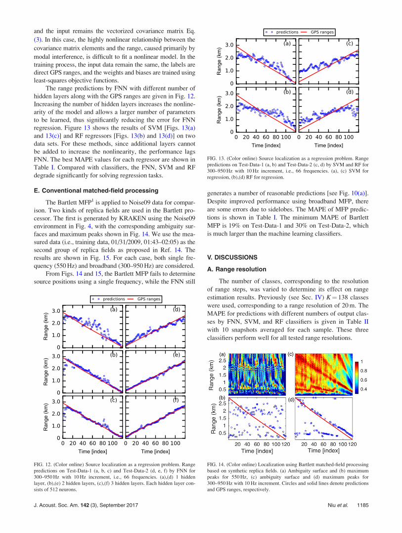
The range predictions by FNN with different number ofhidden layers along with the GPS ranges are given in Fig. 12.Increasing the number of hidden layers increases the nonline-arity of the model and allows a larger number of parametersto be learned, thus significantly reducing the error for FNNregression. Figure 13 shows the results of SVM [Figs. 13(a)and 13(c)] and RF regressors [Figs. 13(b) and 13(d)] on twodata sets. For these methods, since additional layers cannotbe added to increase the nonlinearity, the performance lagsFNN. The best MAPE values for each regressor are shown inTable I. Compared with classifiers, the FNN, SVM and RFdegrade significantly for solving regression tasks.

E. Conventional matched-field processing

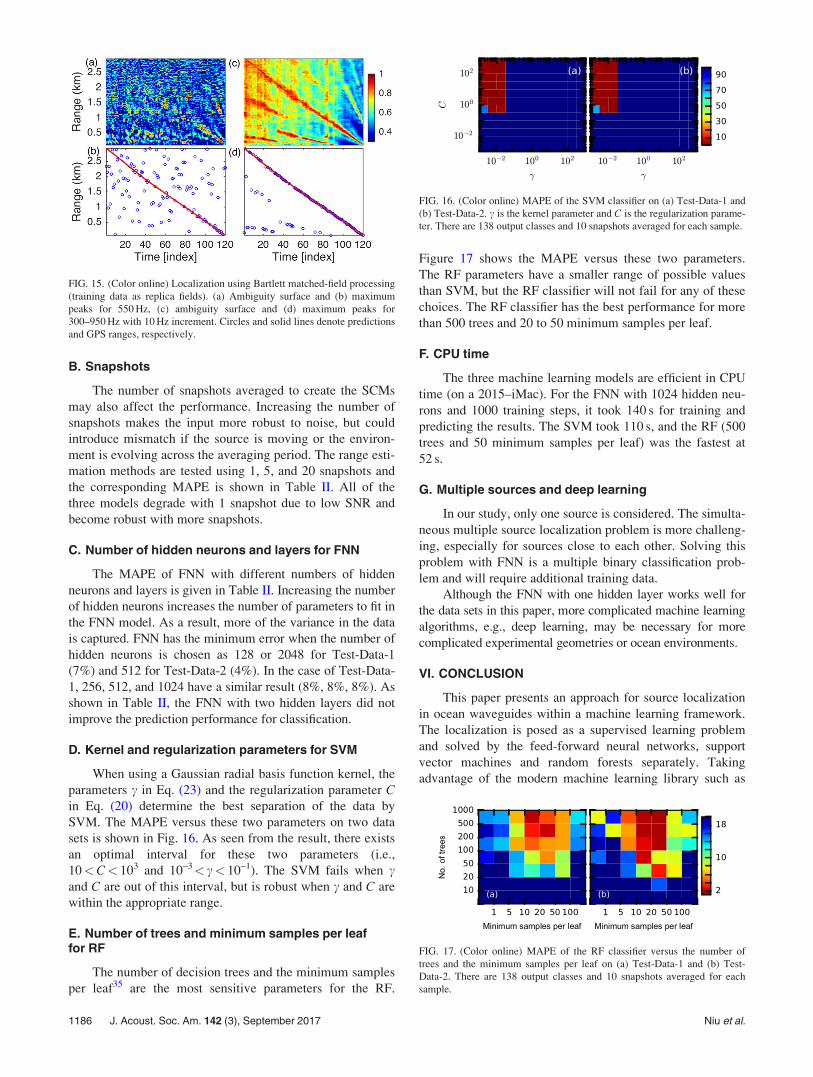
The Bartlett MFP1 is applied to Noise09 data for compar-ison. Two kinds of replica fields are used in the Bartlett pro-cessor. The first is generated by KRAKEN using the Noise09environment in Fig. 4, with the corresponding ambiguity sur-faces and maximum peaks shown in Fig. 14. We use the mea-sured data (i.e., training data, 01/31/2009, 01:43–02:05) as thesecond group of replica fields as proposed in Ref. 14. Theresults are shown in Fig. 15. For each case, both single fre-quency (550 Hz) and broadband (300–950 Hz) are considered.

From Figs. 14 and 15, the Bartlett MFP fails to determinesource positions using a single frequency, while the FNN still

generates a number of reasonable predictions [see Fig. 10(a)].Despite improved performance using broadband MFP, thereare some errors due to sidelobes. The MAPE of MFP predic-tions is shown in Table I. The minimum MAPE of BartlettMFP is 19% on Test-Data-1 and 30% on Test-Data-2, whichis much larger than the machine learning classifiers.

V. DISCUSSIONS

A. Range resolution

The number of classes, corresponding to the resolutionof range steps, was varied to determine its effect on rangeestimation results. Previously (see Sec. IV) K¼ 138 classeswere used, corresponding to a range resolution of 20 m. TheMAPE for predictions with different numbers of output clas-ses by FNN, SVM, and RF classifiers is given in Table IIwith 10 snapshots averaged for each sample. These threeclassifiers perform well for all tested range resolutions.

FIG. 12. (Color online) Source localization as a regression problem. Rangepredictions on Test-Data-1 (a, b, c) and Test-Data-2 (d, e, f) by FNN for300–950 Hz with 10 Hz increment, i.e., 66 frequencies. (a),(d) 1 hiddenlayer, (b),(e) 2 hidden layers, (c),(f) 3 hidden layers. Each hidden layer con-sists of 512 neurons.

FIG. 13. (Color online) Source localization as a regression problem. Rangepredictions on Test-Data-1 (a, b) and Test-Data-2 (c, d) by SVM and RF for300–950 Hz with 10 Hz increment, i.e., 66 frequencies. (a), (c) SVM forregression, (b),(d) RF for regression.

FIG. 14. (Color online) Localization using Bartlett matched-field processingbased on synthetic replica fields. (a) Ambiguity surface and (b) maximumpeaks for 550 Hz, (c) ambiguity surface and (d) maximum peaks for300–950 Hz with 10 Hz increment. Circles and solid lines denote predictionsand GPS ranges, respectively.

J. Acoust. Soc. Am. 142 (3), September 2017 Niu et al. 1185

B. Snapshots

The number of snapshots averaged to create the SCMsmay also affect the performance. Increasing the number ofsnapshots makes the input more robust to noise, but couldintroduce mismatch if the source is moving or the environ-ment is evolving across the averaging period. The range esti-mation methods are tested using 1, 5, and 20 snapshots andthe corresponding MAPE is shown in Table II. All of thethree models degrade with 1 snapshot due to low SNR andbecome robust with more snapshots.

C. Number of hidden neurons and layers for FNN

The MAPE of FNN with different numbers of hiddenneurons and layers is given in Table II. Increasing the numberof hidden neurons increases the number of parameters to fit inthe FNN model. As a result, more of the variance in the datais captured. FNN has the minimum error when the number ofhidden neurons is chosen as 128 or 2048 for Test-Data-1(7%) and 512 for Test-Data-2 (4%). In the case of Test-Data-1, 256, 512, and 1024 have a similar result (8%, 8%, 8%). Asshown in Table II, the FNN with two hidden layers did notimprove the prediction performance for classification.

D. Kernel and regularization parameters for SVM

When using a Gaussian radial basis function kernel, theparameters c in Eq. (23) and the regularization parameter Cin Eq. (20) determine the best separation of the data bySVM. The MAPE versus these two parameters on two datasets is shown in Fig. 16. As seen from the result, there existsan optimal interval for these two parameters (i.e.,10<C< 103 and 10–3< c< 10–1). The SVM fails when cand C are out of this interval, but is robust when c and C arewithin the appropriate range.

E. Number of trees and minimum samples per leaffor RF

The number of decision trees and the minimum samplesper leaf35 are the most sensitive parameters for the RF.

Figure 17 shows the MAPE versus these two parameters.The RF parameters have a smaller range of possible valuesthan SVM, but the RF classifier will not fail for any of thesechoices. The RF classifier has the best performance for morethan 500 trees and 20 to 50 minimum samples per leaf.

F. CPU time

The three machine learning models are efficient in CPUtime (on a 2015–iMac). For the FNN with 1024 hidden neu-rons and 1000 training steps, it took 140 s for training andpredicting the results. The SVM took 110 s, and the RF (500trees and 50 minimum samples per leaf) was the fastest at52 s.

G. Multiple sources and deep learning

In our study, only one source is considered. The simulta-neous multiple source localization problem is more challeng-ing, especially for sources close to each other. Solving thisproblem with FNN is a multiple binary classification prob-lem and will require additional training data.

Although the FNN with one hidden layer works well forthe data sets in this paper, more complicated machine learningalgorithms, e.g., deep learning, may be necessary for morecomplicated experimental geometries or ocean environments.

VI. CONCLUSION

This paper presents an approach for source localizationin ocean waveguides within a machine learning framework.The localization is posed as a supervised learning problemand solved by the feed-forward neural networks, supportvector machines and random forests separately. Takingadvantage of the modern machine learning library such as

FIG. 15. (Color online) Localization using Bartlett matched-field processing(training data as replica fields). (a) Ambiguity surface and (b) maximumpeaks for 550 Hz, (c) ambiguity surface and (d) maximum peaks for300–950 Hz with 10 Hz increment. Circles and solid lines denote predictionsand GPS ranges, respectively.

FIG. 16. (Color online) MAPE of the SVM classifier on (a) Test-Data-1 and(b) Test-Data-2. c is the kernel parameter and C is the regularization parame-ter. There are 138 output classes and 10 snapshots averaged for each sample.

FIG. 17. (Color online) MAPE of the RF classifier versus the number oftrees and the minimum samples per leaf on (a) Test-Data-1 and (b) Test-Data-2. There are 138 output classes and 10 snapshots averaged for eachsample.

1186 J. Acoust. Soc. Am. 142 (3), September 2017 Niu et al.

TensorFlow and Scikit-learn, the machine learning modelsare trained efficiently. Normalized sample covariance matri-ces are fed as input to the models. Simulations show thatFNN achieves a good prediction performance for signalswith SNR above 0 dB even with deficient training samples.Noise09 experimental data further demonstrates the validityof the machine learning algorithms.

Our results show that classification methods performbetter than regression and MFP methods. The three classifi-cation methods tested (FNN, SVM, RF) all performed wellwith the best MAPE 2%–3%. The SVM performs well if themodel parameters are chosen appropriately, otherwise itdegrades significantly. By contrast, the FNN and RF aremore robust on the choices of parameters.

The experimental results show that multi-frequencyinput generates more accurate predictions than single fre-quency (based on FNN). In the current study, the trainingand test data were from the same ship. In a realistic applica-tion, data from multiple ships of opportunity can be used astraining data by taking advantage of the AutomaticIdentification System (AIS), a GPS system required on allcargo carriers. The tracks were quite similar and it would beinteresting to compare the performance of the three methodsas tracks deviate.

ACKNOWLEDGMENTS

This work was supported by the Office of NavalResearch under Grant No. N00014–1110439 and the ChinaScholarship Council.

1F. B. Jensen, W. A. Kuperman, M. B. Porter, and H. Schmidt,Computational Ocean Acoustics, 2nd ed. (Springer Science & BusinessMedia, New York, 2011), Chap. 10.

2H. P. Bucker, “Use of calculated sound fields and matched field detectionto locate sound source in shallow water,” J. Acoust. Soc. Am. 59, 368–373(1976).

3H. Schmidt, A. B. Baggeroer, W. A. Kuperman, and E. K. Scheer,“Environmentally tolerant beamforming for high-resolution matched fieldprocessing: Deterministic mismatch,” J. Acoust. Soc. Am. 88, 1851–1862(1990).

4M. D. Collins and W. A. Kuperman, “Focalization: Environmental focus-ing and source localization,” J. Acoust. Soc. Am. 90, 1410–1422 (1991).

5E. K. Westwood, “Broadband matched-field source localization,”J. Acoust. Soc. Am. 91, 2777–2789 (1992).

6A. B. Baggeroer, W. A. Kuperman, and P. N. Mikhalevsky, “An overviewof matched field methods in ocean acoustics,” IEEE J. Ocean. Eng. 18,401–424 (1993).

7D. F. Gingras and P. Gerstoft, “Inversion for geometric and geoacousticparameters in shallow water: Experimental results,” J. Acoust. Soc. Am.97, 3589–3598 (1995).

8Z. H. Michalopoulou and M. B. Porter, “Matched-field processing forbroad-band source localization,” IEEE J. Ocean. Eng. 21, 384–392 (1996).

9C. F. Mecklenbra€uker and P. Gerstoft, “Objective functions for oceanacoustic inversion derived by likelihood methods,” J. Comput. Acoust. 8,259–270 (2000).

10C. Debever and W. A. Kuperman, “Robust matched-field processing usinga coherent broadband white noise constraint processor,” J. Acoust. Soc.Am. 122, 1979–1986 (2007).

11S. E. Dosso and M. J. Wilmut, “Bayesian multiple source localization inan uncertain environment,” J. Acoust. Soc. Am. 129, 3577–3589 (2011).

12S. E. Dosso and M. J. Wilmut, “Maximum-likelihood and other processorsfor incoherent and coherent matched-field localization,” J. Acoust. Soc.Am. 132, 2273–2285 (2012).

13S. E. Dosso and M. J. Wilmut, “Bayesian tracking of multiple acousticsources in an uncertain ocean environment,” J. Acoust. Soc. Am. 133,EL274–EL280 (2013).

14L. T. Fialkowski, M. D. Collins, W. A. Kuperman, J. S. Perkins, L. J.Kelly, A. Larsson, J. A. Fawcett, and L. H. Hall, “Matched-field process-ing using measured replica fields,” J. Acoust. Soc. Am. 107, 739–746(2000).

15C. M. A. Verlinden, J. Sarkar, W. S. Hodgkiss, W. A. Kuperman, and K.G. Sabra, “Passive acoustic source localization using sources of oppor-tunity,” J. Acoust. Soc. Am. 138, EL54–EL59 (2015).

16Z. Lei, K. Yang, and Y. Ma, “Passive localization in the deep ocean basedon cross-correlation function matching,” J. Acoust. Soc. Am. 139,EL196–EL201 (2016).

17H. C. Song and Chomgun Cho, “Array invariant-based source localizationin shallow water using a sparse vertical array,” J. Acoust. Soc. Am. 141,183–188 (2017).

18R. Lefort, G. Real, and A. Dr"emeau, “Direct regressions for underwateracoustic source localization in fluctuating oceans,” Appl. Acoust. 116,303–310 (2017).

19G. Hinton, L. Deng, D. Yu, G. E. Dahl, A. Mohamed, N. Jaitly, A.Senior, V. Vanhoucke, P. Nguyen, T. N. Sainath, and B. Kingsbury,“Deep neural networks for acoustic modeling in speech recognition: Theshared views of four research groups,” IEEE Signal Proc. Mag. 29, 82–97(2012).

20A. Krizhevsky, I. Sutskever, and G. E. Hinton, “Imagenet classificationwith deep convolutional neural networks,” Adv. Neural Inf. Process. Syst.1097–1105 (2012).

21R. Collobert, J. Weston, L. Bottou, M. Karlen, K. Kavukcuoglu, and P.Kuksa, “Natural language processing (almost) from scratch,” J. Mach.Learn. Res. 12, 2493–2537 (2011).

22M. L. Sharma and M. K. Arora, “Prediction of seismicity cycles in thehimalayas using artificial neural networks,” Acta Geophys. Polonica 53,299–309 (2005).

23S. R. Garc"ıa, M. P. Romo, and J. M. Mayoral, “Estimation of peak groundaccelerations for Mexican subduction zone earthquakes using neuralnetworks,” Geofis. Int. 46, 51–63 (2006).

24A. K€ohler, M. Ohrnberger, and F. Scherbaum, “Unsupervised pattern rec-ognition in continuous seismic wavefield records using Self-OrganizingMaps,” Geophys. J. Int. 182, 1619–1630 (2010).

25N. Riahi and P. Gerstoft, “Using graph clustering to locate sources withina dense sensor array,” Signal Process. 132, 110–120 (2017).

26B. Z. Steinberg, M. J. Beran, S. H. Chin, and J. H. Howard, “A neural net-work approach to source localization,” J. Acoust. Soc. Am. 90, 2081–2090(1991).

27J. M. Ozard, P. Zakarauskas, and P. Ko, “An artificial neural network forrange and depth discrimination in matched field processing,” J. Acoust.Soc. Am. 90, 2658–2663 (1991).

28A. Caiti and T. Parisini, “Mapping ocean sediments by RBF networks,”IEEE J. Ocean. Eng. 19, 577–582 (1994).

29A. Caiti and S. Jesus, “Acoustic estimation of seafloor parameters: Aradial basis functions approach,” J. Acoust. Soc. Am. 100, 1473–1481(1996).

30Y. Stephan, X. Demoulin, and O. Sarzeaud, “Neural direct approaches forgeoacoustic inversion,” J. Comput. Acoust. 6, 151–166 (1998).

31J. Benson, N. R. Chapman, and A. Antoniou, “Geoacoustic model inversionusing artificial neural networks,” Inverse Problems 16, 1627–1639 (2000).

32Z. H. Michalopoulou, D. Alexandrou, and C. Moustier, “Application ofneural and statistical classifiers to the problem of seafloor character-ization,” IEEE J. Ocean. Eng. 20, 190–197 (1995).

33A. M. Thode, K. H. Kim, S. B. Blackwell, C. R. Greene, C. S. Nations, T.L. McDonald, and A. M. Macrander, “Automated detection and localiza-tion of bowhead whale sounds in the presence of seismic airgun surveys,”J. Acoust. Soc. Am. 131, 3726–3747 (2012).

34M. Abadi, A. Agarwal, P. Barham, E. Brevdo, Z. Chen, C. Citro, G. S.Corrado, A. Davis, J. Dean, M. Devin, S. Ghemawat, I. Goodfellow, A.Harp, G. Irving, M. Isard, Y. Jia, R. Jozefowicz, L. Kaiser, M. Kudlur, J.Levenberg, D. Man"e, R. Monga, S. Moore, D. Murray, C. Olah, M.Schuster, J. Shlens, B. Steiner, I. Sutskever, K. Talwar, P. Tucker, V.Vanhoucke, V. Vasudevan, F. Vi"egas, O. Vinyals, P. Warden, M.Wattenberg, M. Wicke, Y. Yu, and X. Zheng, “TensorFlow: Large-scalemachine learning on heterogeneous distributed systems,” Software avail-able from tensorflow.org (2015).

35F. Pedregosa, G. Varoquaux, A. Gramfort, V. Michel, B. Thirion, O.Grisel, M. Blondel, P. Prettenhofer, R. Weiss, V. Dubourg, J. Vanderplas,A. Passos, D. Cournapeau, M. Brucher, M. Perrot, and "E. Duchesnay,“Scikit-learn: Machine learning in Python,” J. Mach. Learn. Res. 12,2825–2830 (2011).

J. Acoust. Soc. Am. 142 (3), September 2017 Niu et al. 1187

36J. Bergstra, O. Breuleux, F. Bastien, P. Lamblin, R. Pascanu, G.Desjardins, J. Turian, D. Warde-Farley, and Y. Bengio, “Theano: A CPUand GPU math compiler in Python,” Proc. 9th Python in Science Conf.(2010), pp. 1–7.

37Y. Jia, E. Shelhamer, J. Donahue, S. Karayev, J. Long, R. Girshick, S.Guadarrama, and T. Darrell, “Caffe: Convolutional architecture for fastfeature embedding,” in Proceedings of 22nd ACM international confer-ence on Multimedia (2014), pp. 675–678.

38R. Collobert, S. Bengio, and J. Mari"ethoz, “Torch: A modular machinelearning software library,” No. EPFL-REPORT-82802, Idiap (2002).

39D. Kingma and B. Jimmy, “Adam: A method for stochastic optimization,”arXiv preprint arXiv:1412.6980 (2014).

40N. Srivastava, G. E. Hinton, A. Krizhevsky, I. Sutskever, and R.Salakhutdinov, “Dropout: A simple way to prevent neural networks fromoverfitting,” J. Mach. Learn. Res. 15, 1929–1958 (2014).

41C. M. Bishop, Pattern Recognition and Machine Learning (Springer, NewYork, 2006), Chaps. 4, 5, and 7.

42R. Fan, P. Chen, and C. Lin, “Working set selection using second orderinformation for training support vector machines,” J. Mach. Learn. Res. 6,1889–1918 (2005).

43L. Breiman, “Random forests,” Mach. Learn. 45, 5–32 (2001).44L. Breiman, “Bagging predictors,” Mach. Learn. 24, 123–140 (1996).45P. Goodwin and R. Lawton, “On the asymmetry of the symmetric

MAPE,” Int. J. Forecasting 15, 405–408 (1999).46M. B. Porter, The KRAKEN Normal Mode Program, http://oalib.hlsresearch.

com/Modes/AcousticsToolbox/manualtml/kraken.html (Last viewed 11/1/2009).

47S. H. Byun, C. M. A. Verlinden, and K. G. Sabra, “Blind deconvolution ofshipping sources in an ocean waveguide,” J. Acoust. Soc. Am. 141,797–807 (2017).

1188 J. Acoust. Soc. Am. 142 (3), September 2017 Niu et al.