Sources and Further Readings

Chapter 1: The Taming of Chance

The introduction to probability and statistics in this chapter is

thoroughly elementary and intuitive. Among the many ele­

mentary accounts of statistics, a particularly clear treatment is

provided in Statistics, a book by Freedman, Pisani, Purves, and

Adhikari [29]. To my mind the most authoritative and provoca­

tive book on probability remains the classic work An Introduction

to Probability Theory and its Applications of William Feller [27],

where among other topics one will find proofs of Bernoulli's

Law of Large Numbers and de Moivre's theorem regarding the

normal, or Gaussian, curve. Although Feller's book is very en­

gaging, it is not always easy reading for the beginner.

145

Sources and Further Readings

There are two delightful articles by Mark Kac called "What

Is Random?" [37] that prompted the title of this book, and

"Probability" [38]. There are several additional articles on

probability in the collection The World ojMathematics, edited by

James Newman some years ago [52]. I especially recommend

the passages translated from the works of James Bernoulli,

Pierre Simon Laplace (from which I also cribbed a quotation),

and Jules-Henri Poincare. The Francis Galton quotation also

comes from Newman's collection, in an essay by Leonard Tip­

pett called "Sampling and Sampling Error," and Laplace's

words are from a translation of his 1814 work on probability in

the same Newman set. A philosophical perspective on proba­

bility, called simply "Chance," is by AlfredJ. Ayer [3].

Technical accounts of statistical tests of randomness, in­

cluding the runs test, are in the second volume of Donald

Knuth's formidable magnum opus Seminumerical Algorithms [42].

The idea of chance in antiquity is documented in the book

Gods, Games, and Gambling by Florence David [22], while the

rise and fall of the goddess Fortuna is recounted in a book by

Howard Patch [54], from which I took a quotation. Oystein

Ore has written an engaging biography of Girolamo Cardano,

including a translation of Liber de Ludo Aleae, in Cardano, the

Gambling Scholar [53]. A spirited and very readable account of

how the ancients conceptualized the idea of randomness and

how this led to the origins of probability is provided in Debo­

rah Bennett's attractive book called Randomness [8]. The early history of the rise of statistics in the service of

government bureaucracies during the eighteenth and nine-

146

Sources and Further Readings

teenth centuries is fascinatingly told by Ian Hacking [35] in a

book whose title I shamelessly adopted for the present chapter.

I also recommend the entertaining book Against the Gods, by

Peter Bernstein [12], that takes particular aim at the notion of

chance and risk in the world of finance.

The perception of randomness as studied by psychologists is

summarized in an article by Maya Bar-Hillel and Willem Wage­

naar [6]. More will be said about this topic in the next chapter.

Chapter 2: Uncertainty and Information

The story of entropy and information and the importance of

coding is the subject matter of information theory. The original

paper by Claude Shannon is tough going, but there is a nice ex­

pository article by Warren Weaver that comes bundled with a

reprint of Shannon's contribution in the volume The Mathemati­cal Theory q{Communication [62]. There are several other reason­

ably elementary expositions that discuss a number of the topics

covered in this chapter, including those of Robert Lucky [45]

and John Pierce [56]. An up-to-date but quite technical version

is Thomas Cover and Joy Thomas's Elements q{Information Theory

[20]. A fascinating account of secret codes is David Kahn's The

Code-Breakers [39]. There are readable accounts of the investi­

gations of psychologists in the perception of randomness by

Ruma Falk and Clifford Konold [26] and Daniel Kahneman

and Amos Tversky [40], in addition to the previously cited

paper by Maya Bar-Hillel and Willem Wagenaar [6].

147

Sources and Further Readings

Approximate entropy is discussed in an engagingly simple

way by Fred Attneave in a short monograph called Applications

oJlnformation Theory to Psychology [2]. Extensions and ramifica­

tions of this idea, as well as the term ApEn, can be found in

"Randomness and Degrees of Irregularity" by Steve Pincus

and Burton Singer [57] and "Not All (Possibly) 'Random' Se­

quences Are Created Equal" by Steve Pincus and Rudolf

Kalman [58]. Among other things, these authors do not re­

strict themselves to binary sequences, and they permit arbi­

trary source alphabets. An elementary account of this more re­

cent work in John Casti's "Truly, Madly, Randomly" [14].

Chapter 3: Janus-Faced Randomness

The Janus algorithm was introduced in Bardett's paper

"Chance or Chaos" [7]. A penetrating discussion of the mod 1

iterates and chaos is available in Joseph Ford's "How Random

Is a Coin Toss?" [28].

Random number generators are given a high-level treat­

ment in Donald Knuth's book [42], but this is recommended

only to specialists. A more accessible account is in Ivar Eke­

land's charming book The Broken Dice [25]. The quotation from George Marsaglia is the tide of his

paper [49].

Maxwell's and Szilard's demons are reviewed in two papers

having the same tide, "Maxwell's Demon," by Edward Daub

[21] and W. Ehrenberg [24]. There is also a most informative

paper by Charles Bennett called "Demons, Engines, and the

148

Sources and Further Readings

Second Law" [9]. The slim volume Chance and Chaos, by David

Ruelle [60], provides a simplified introduction to many of the

same topics covered here and in other portions of our book.

George Johnson's fast-paced and provocative book Fire in the Mind [36] also covers many of the topics in this and the next

two chapters, and is especially recommended for its com­

pelling probe of the interface between science and faith.

Chapter 4: Algorithms, Information, and Chance

I have glossed over some subtleties in the discussion of algorith­

mic complexity, but the dedicated reader can always refer to the

formidable tome by Li and Vitanyi [44], which also includes ex­

tensive references to the founders of this field several decades

ago, including the American engineer Ray Solomonotf, who,

some believe, may have launched the entire inquiry.

There is an excellent introduction to Turing machines

and algorithmic randomness in "What Is a Computation," by

Martin Davis [23], in which he refers to Turing-Post pro­

grams because of the related work of the logician Emil Post.

An even more detailed and compelling account is by Roger

Penrose in his book Shadows if the Mind [55], and my proof

that the halting problem is undecidable in the technical notes

is taken almost verbatim from this source.

The best introduction to Gregory Chaitin's work is by

Chaitin himself in an article called "Randomness and Math­

ematical Proof" [16] as well as the slightly more technical

149

Sources and Further Readings

"Information-Theoretic Computational Complexity" [17].

Chaitin's halting probability n is described in an IBM report

by Charles Bennett called "On Random and Hard-to­

Describe Numbers" [11), which is engagingly summarized by

Martin Gardner in "The Random Number n Bids Fair to

Hold the Mysteries of the Universe" [31]. The Bennett quo­

tation is from these sources.

The distinction between cause and chance as generators of

a string of data is explored more fully in the book by Li and Vi­

tanyi mentioned above.

The words of Laplace are from a translation of his 1814

Essai philosophique sur les probabilites, but the relevant passages

come from the excerpt by Laplace in Newman's World if Mathematics [52]. The Heisenberg quotation is from the article

"Beauty and the Quest for Beauty in Science," by S. Chan­

drasekhar [18].

The work ofW.H. Zurek that was alluded to is summa­

rized in his paper "Algorithmic Randomness and Physical En­

tropy" [67].

Quotations from the writing of Jorge Luis Borges were

extracted from his essays "Partial Magic in the Quixote" and

"The Library of Babel," both contained in Labyrinths [13).

Chapter 5: The Edge of Randomness

Charles Bennett's work on logical depth is found in a fairly

technical report [10]. A sweeping overview of many of the

topics in this section, including the contributions of Bennett,

150

Sources and Further Readings

is The Quark and the Jaguar, by Murray Gell-Mann [32].

Jacques Monod's influential book is called Chance and Necessity

[51]. Robert Frost's arresting phrase is from his essay "The

Figure a Poem Makes" [30], and Jonathan Swift's catchy verse

is from his "On Poetry, a Rhapsody" and is quoted in Man­

delbrot's book [47].

The quotations from Stephen Jay Gould come from sev­

eral of his essays in the collection Eight Little Piggies [34]. His

view on the role of contingency in the evolutionary history of

living things is summarized in the article "The Evolution of

Life on the Earth" [33]. The other quotations come from the

ardently written books How Nature Works [4], by Per Bak, and

At Home in the Universe, by Stuart Kauffinan [41]. Ilya Pri­

gogine's thoughts on nonequilibrium phenomena are con­

tained in the celebrated Order Out oj Chaos, which he wrote

with Isabelle Stengers [59]. Cawelti's book is Adventure, Mys­tery, and Romance [15]. A useful resume of the work of Watts

and Strogatz is in "It's a Small World" by James Collins and

Carson Chow [19].

Benoit Mandelbrot's astonishing book is called The Fractal Geometry oJNature [47]. Some of the mathematical details that

I left unresolved in the text are provided in a rather technical

paper by Mandelbrot and Van Ness [48].

Other, more accessible, sources to self-similarly, l/flaws,

and details about specific examples are noted in Bak's book

mentioned above; the article "Self-organized Criticality," by

Per Bak, Kan Chen, and Kurt Wiesenfeld [5]; Stephan

Machlup's "Earthquakes, Thunderstorms, and Other iff

151

Sources and Further Readings

Noises" [46]; "The Noise in Natural Phenomena," by Bruce

West and Michael Shlesinger [65]; "Physiology in Fractal Di­

mensions," by Bruce West and Ary Goldberger [66]; and the

books Fractals and Chaos, by Larry Leibovitch [43], and Man­

fred Schroeder's Fractals, Chaos, and Power LAws [61]. All of the

quotations come from one or the other of these sources.

Music as pink noise is discussed in "1/1Noise in Music;

Music from 1/1 Noise," by Richard Voss and John Clarke

[64]. The plankton data are from [1].

152

Technical Notes

The following notes are somewhat more technical in nature

than the rest of the book and are intended for those readers

with a mathematical bent who desire more details than were

provided in the main text. The notes are strictly optional,

however, and in no way essential for following the the main

thread of the discussion in the preceeding chapters.

Chapter 1: The Taming of Chance

1.1.

The material under this heading is optional and is intended to

give the general reader some specific examples to illustrate the

probability concepts that were introduced in the first chapter.

153

Technical Notes

In three tosses of a coin, the sample space S consists of 8

possible outcomes HHH, HHT, HTH, THH, THT, TTH,

HTT, TTT, with H for head and T for tail. The triplets define

mutually exclusive events, and since they are all equally likely,

each is assigned probability Ys. The composite event "two

heads in three tosses" is the subset of S consisting of HHT,

HTH, THH (with probability %), and this is not mutually ex­

clusive of the event "at least two heads in three tosses" since the

latter event consists of the three triplets HHT, HTH, THH

plus HHH (with probability % = %). In the example above, HHT and HTH are mutually ex­

clusive events, and the probability of one or the other happen­

ing is Ys + Ys = Y4. By partitioning S into a bunch of exclusive events, the sum of the probabilities of each of these disjoint

sets of possibilities must be unity, since one of them is certain

to occur.

The independence of events A and B is expressed mathemati­

cally by stipulating that the event "both A and B take place" is the product of the separate probabilities of A and B. Thus, for ex­

ample, in three tosses of a fair coin, the events "first two tosses

are heads" and "the third toss is head," which are denoted re­

spectively by A and B, are intuitively independent, since there

is a fifty-fifty chance of getting a head on any given toss re­

gardless of how many heads preceded it. In fact, since A con­

sists of HHH and HHT, while B is HHH, HTH, THH,

TTH, it follows that the probability of A = % = % and the

probability ofB = 'Ys = %; however, the probability that "both

A and B takes place" is Ys, since this event consists only of

154

Technical Notes

HHH. Observe that the product of the probabilities of A and

B is Y4 times ~, namely Va. One can also speak of events conditional on some other

event having taken place. When the event F is known to have

occurred, how does one express the probability of some other

event E in the face of this information about F? To take a spe­

cific case, let us return to the sample space of three coin tosses

considered in the previous paragraph and let F represent "the

first toss is a head." Event F has probability ~, as a quick scan

of the 8 possible outcomes shows. Assuming that F is true re­

duces the sample space S to only four elementary events HTT,

HTH, HHT, HHH. Now let E denote "two heads in 3

tosses." The probability of E equals 318 ifF is not taken into ac­

count. However, the probability of E given that F has in fact

taken place is ~, since the number of possibilities has dwindled

to the two cases HHT and HTH out of the four in F. The

same kind of reasoning applies to any finite sample space and

leads to the conditional probability of E given F. Note that if E and F are independent, then the conditional probability is sim­

ply the probability of E, because a knowledge ofF is irrelevant

to the happening or nonhappening ofE.

1.2.

This technical aside elaborates on the interpretation of infi­

nite sample spaces of unlimited Bernoulli Y2-trials that began

with the discussion of the Strong Law of Large Numbers.

Though not necessary for what follows in the book, it offers

the mathematically inclined reader some additional insights

155

Technical Notes

into the underpinnings of modern probability theory. I will

use some mathematical notions that may already be familiar to

you, but in any case I recommend that you consult Appen­

dices A and B, which cover the required background material

in more detail.

The set of all numbers in the unit interval between zero

and one can be identified in a one-to-one manner with the set

of all possible nonterminating strings of zeros and ones, pro­

vided that strings with an unending succession of ones are

avoided. The connection is that any x in the unit interval can

be written as a sum

where each ak , k = 1,2 ... , denotes either 0 or 1. For exam­

ple, 3/8 = %1 + Yz2 + Yz3, with the remaining terms all zero.

The number x is now identified with the infinite binary string

a1a2a3" ... With this convention, x = ~ corresponds to the

string 011 00 .... Similarly, % = 01010101. ... In some cases

two representations are possible, such as Y4 = 01000 ... and Y4 = 00111 ... , and when this happens we opt for the first pos­

sibility. So far, this paraphrases Appendix B, but now comes

the connection to probability.

Each unending sequence of Bernoulli Yz-trials gives rise to

an infinite binary string and therefore to some number x in the

unit interval. Let S be the sample space consisting of all possi­

ble strings generated by this unending random process. Then

an event E in S is a subset of such strings, and the probability of E is taken to be the length of the subset of the unit interval that corre-

156

Technical Notes

sponds to E. Any two subsets of identical length correspond to

events having the same probability.

If the subset consists of nonoverlapping intervals within

the unit interval, then its length is the sum of the lengths of the

individual subintervals. For more complicated subsets, the no­

tion oflength becomes problematical, and it is necessary to in­

voke the concept of measure (see the discussion below, later in

this note).

Conversely, any x in the unit interval gives rise to a string

generated by a Bernoulli V2-process. In fact, if x corresponds to

a1a2a3 .•. , then a1 = ° if and only if x belongs to the subset [0,

Vz), which has length V2• This means that the probability of a1

being zero is V2; the same applies if a1 = 1. Now consider a2•

This digit is ° if and only if x belongs to either [0, %) or [V2, 3/4).

The total length of these disjoint intervals is V2, and since they

define mutually exclusive events, the probability of a2 being

zero is necessarily V2. Obviously, the same is true if a2 = 1.

Proceeding in this fashion it becomes evident that each ak, for

k = 1, 2, ... , has an equal probability of being zero or one.

Note that regardless of the value taken on by a1, the probabil­

ity of a2 remains Vz, and so a1 and a2 are independent. The same

statistical independence applies to any succession of these dig­

its. It follows that the collection qf numbers in the unit interval is

identified in a one-to-one fashion with all possible outcomes qfBemoulli

Y2-trials.

If s is a binary string oflength n, let fs denote the set of all infinite strings that begin with s. Now, s itself corresponds to

some terminating fraction x, and since the first n positions of

157

Technical Notes

the infinite string have already been specified, the remaining

digits sum to a number whose length is at most lizn. To see this,

first note that any sum of terms of the form aJ2k can never ex­

ceed in value a similar sum of terms lizk, since ak is always less

than or equal to one. Therefore the infinite sum of terms ak/2k

starting from k = n + 1 is at most equal to the corresponding

sum of terms W, and as Appendix A demonstrates, this last

sum is simply lizn. Therefore, the event fs corresponds to the interval be­

tween x and x + V2n, and this interval has length lizn. It follows

that the event fs has probability lizn. Thus, ifE is the event "all

strings whose first three digits are one," then E consists of all

numbers that begin with liz + ~ + Vs = 7/s, and this gives rise

to the interval between Vs and 1, whose length is Ys. Therefore

the probability of E is Ys. If you think of the fs as elementary

events in S, then they are uniformly distributed, since their

probabilities are all equal.

There is a technical complication here regarding what is

meant by the length of a subset when the event E is so con­

trived that it does not correspond to an interval in the ordinary

sense. However, a resolution of this issue would get us tied up

in the nuances of what is known in mathematics as measure the­

ory, a topic that need not detain us. For our purposes it is

enough to give a single illustration to convey the essence of

what is involved. Let E denote "the fourth trial is a zero." This

event is realized as the set all strings whose first three digits are

one of the 23 = 8 possibilities 111, 11 0, ... , 000 and whose

fourth digit is zero. Each of these possibilities corresponds to a

158

Technical Notes

number that begins in one of8 distinct locations in the unit in­

terval and extends for length Y16 to the right. For example,

1010 represents the number %, and the remaining sequence

sums to at most another Y16. It follows that E is the union of8

disjoint events, each oflength Y16, summing to ~, and this is

the probability of E (again, a more detailed discussion can be

found in Appendix A).

An unexpected feature of this infinite sample space is that

since probability zero must correspond to a set of zero

"length," called measure zero, it is possible that an event of zero

probability may itself correspond to an infinite collection of

strings! To see this we consider the subset R of all rational

numbers (namely, common fractions) in the unit interval.

These fractions can be written as an infinite sequence of infinite

sequences in which the numerator is first 1, then 2, and so on:

~,Y3, %, .. . %, %, 2;4, .. .

%, %, 3/5, •••

With a zigzag tagging procedure these multiple arrays of

fractions can be coalesced into a single infinite sequence of ra­

tional numbers, as described in the ninth chapter oflan Stew­

art's introductory book [63]. Omitting repetitions, the first

few elements of this sequence are ~, %, %, %, %, Ys, %, ... Let E be an arbitrarily small positive number and enclose

the nth element of the sequence within an interval oflength E

159

Technical Notes

times Y2n for n = 1,2, .... Then R is totally enclosed within a

set S whose total length cannot exceed E times the sum % + Yi + %3 + ... , which (Appendix A again!) is simply E. But E

was chosen to be arbitrarily small, and therefore the "length,"

or measure, of S must necessarily be zero. The probability of

"a string corresponds to a rational number" is consequently

zero. In the language of measure theory it is often stated that an

event has probability 1 ifit holds "almost everywhere," that is,

except for a negligible subset of measure zero.

For balanced coins (p = %), the content of the Strong Law

of Large Numbers is that Sn/n differs from Y2 by an arbitrarily

small amount for all large enough n, except for a subset of un­

limited Bernoulli %-trials having measure zero. This is the

caveat that I mentioned earlier, formulated now in the lan­

guage of measure theory.

I can now restate the assertion made in the text about nor­

mal numbers by saying that all numbers are normal except for a set

if measure zero.

1.3.

The simple MA TLAB m-file below is for those readers with

access to MA TLAB who wish to generate Bernoulli p-trials

for their own amusement:

% CODE TO GENERATE SEQUENCES

% FROM A BERNOULLI P-PROCESS. The output

% is a binary string oflength n.

160

2.1.

Technical Notes

n = input('string size is ... ');

P = input('probability of a success is ... ');

ss = [];

for k = 1: n

if rand < p

s = 1;

else s = 0; end

ss = [ss, s];

end

ss

Chapter 2: Uncertainty and Information

The following comments are intended to clarity the discussion

of message compression when there are redundancies.

The Law of Large numbers discussed in the previous

chapter asserts that in a long enough sequence of n Bernoulli

p-trials with a likelihood p of a success (namely a one) on any

trial, the chance that the proportion of successes Snln deviates

from p by an arbitrarily small amount is close to unity. What

this says, in effect, is that in a long binary string, it is very likely

that the number of l' s, which is S n' will nearly equal np, and of

course, the number ofO's will nearly equal n(l - p). The odds

are then overwhelmingly in favor of such a string being close

161

Technical Notes

to a string in which the digit one appears np times and the

digit zero appears n(l - p) times. This is because successive

Bernoulli trials are independent, and as we know, the proba­

bility of a particular string of independent events, namely the

choice of zero or one, must equal the product of the probabil­

ities of the individual events. The product in question is

pnp (1 - p)n(1-p),

and it is equal to 1/2nh for some suitable h yet to be determined.

Taking logarithms to the base two of both sides (see Appen­

dix q, we obtain

np logp + n(l - p) 10g(1 - p) = -nh log 2.

One can now solve for h and obtain, noting that log 2 = 1,

h = -[p logp + (1 - p) 10g(1 - p)],

which is the entropy H of the source. It is therefore likely that

a binary string oflength n has very nearly a probability 2 -nH of

occurring. Stated differently, the fraction of message strings

having a probability 2 -nH of appearing is nearly one. It follows

that there must be altogether about 2nH such message strings,

and it is highly improbable that an actual message sequence is

not one of them. Even so, these most likely messages consti­

tute a small fraction of the 2 n strings that are possible, since

2 nH/2 n is tiny for large n. An exception to this is when p = ~

because H equals unity in that case.

As a postscript to this argument I remind you that the Strong

Law of Large Numbers asserts that in an infinite sequence of

162

Technical Notes

Bernoulli p-trials, ones and zeros occur with frequencies p and

1 - P with probability one. It should be fairly plausible now that

"probability one" corresponds to "measure zero," as it was de­

fined in the technical note 1.2, whenever p does not equal ~.

2.2.

This note expands on the Shannon coding scheme.

An alphabet source has k symbols whose probabilities of

occurrence Pt' P2' ... ,Pk are assumed to be listed in decreasing

order. Let Pr denote the sum Pt + ... + Pr-1' for r = 1, ... ,k, with P t set to 0. The binary expansion of Pr is a sum aJ2i, for i

= 1,2, ... (Appendix B). Truncate this infinite sum when i is the first integer, call it ir, that is no smaller than -logpr and, by

default, less than 1 - logp,. The binary code for rth symbol is

then the string at a2 ••• ar'

For example, for a source alphabet a, h, c, and d with cor­

responding probabilities ~, Y4, Ys, and Ys, P t = 0, P2 = ~ + 0/22, P3 = ~ + ~2 + %\ and P4 = ~ + Yi + ~3. Now, -log

~ = 1, -log ~2 = 2, and -log ~3 = 3, and so, following the

prescription given above, the code words for the source sym­

bols a, h, c, and dare 0, 10, 110, 111, respectively, with lengths

1,2,3, and 3.

For s = r + 1, ... , k the sum Ps is no less than Pr+ l' which,

in turn, equals Pr + Pr' As you saw, -logpr is less than or equal

to ir, which is equivalent to stating that Pr is no less than Wr (see

Appendix C for details on manipulating logarithms). There­

fore, the binary expansion of Ps differs from that of Pr by at least

one digit in the first ir places, since Wr is being added in. If the

163

Technical Notes

last digit of Pr is 0, for instance, adding 1/21r changes this digit

to 1. This shows that each code word differs from the others,

and so the k words together are a decodable prefix code. This

is certainly true of the illustration above, in which the code is

0, 10, 110, 111.

The Shannon code assigns short words to symbols of

high probability and long codes to symbols oflow probabil­

ity. The average code length L is defined to be the sum over

r of IrPr' and the discussion above now readily establishes that

L is no smaller than-sum of Pr 10gPr and certainly less than the

sum of (p r - P r log p,). The probabilities P r add to 1 for r = 1,

... , k, since the symbols represent mutually exclusive

choices. Also, you recognize the sums on the extreme right

and left as the entropy H of the source. Putting everything

together, therefore, we arrive at the statement that average

code length of the Shannon prefix code differs from the en­

tropy, the average information content of the source, by no

more than 1. A message string from a source of entropy H

can therefore be encoded, on average, with nearly H bits per

symbol.

2.3.

In defining ApEn(k) an alternative approach would be to for­

mally compute the conditional entropy of a k-gram given that we

know its first k-l entries. This expression, which is not de­

rived here, can be shown to equal H(k) - H(k - 1), and this is

identical to the definition of ApEn(k) in the text.

164

Technical Notes

2.4.

A simple program written as a MA TLAB m-file implements

the ApEn algorithm for k up to 4, and is included here for

those readers who have access to MA TLAB and would like to

test their own hand-tailored sequences for randomness.

% CODE TO TEST FOR RANDOMNESS

% IN ZERO-ONE STRINGS

% input is digit string u as a column oflength n

% and a block length k that is no greater than 4.

%

% the matrix below is used in the computation:

%

A = [1 1 1 1 1 1 1 1 00000000

1111000011110000 1100110011001100

1 0 1 0 1 0 1 0 1 0 1 0 1 0 1 0];

%

ApEn = []; h = []; form = l:k

N = n - m + 1;

P = 2A m;

Q = A(1:m, 1:2A(4 - m):16);

U = zeros(N,p);

r = zeros(1,p);

forj = 1:p

fori = 1:N

165

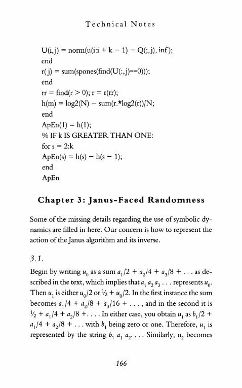
Technical Notes

U(i,j) = norm(u(i:i + k - 1) - Q(;,j), inf);

end

r(j) = sum(spones(find(U(:,j)==O)));

end

rr = find(r > 0); r = r(rr);

h(m) = log2(N) - sum(r.*log2(r))/N;

end

ApEn(l) = h(l);

% IF k IS GREATER THAN ONE:

for s = 2:k

ApEn(s) = h(s) - h(s - 1);

end

ApEn

Chapter 3: Janus-Faced Randomness

Some of the missing details regarding the use of symbolic dy­

namics are filled in here. Our concern is how to represent the

action of the Janus algorithm and its inverse.

3.1.

Begin by writing Uo as a sum ad2 + a2/4 + a3/8 + ... as de­

scribed in the text, which implies that at a2 a3 ••• represents uo.

Then ut is either uo/2 or % + uo/2. In the first instance the sum

becomes a t /4 + a2/8 + a3/16 + ... , and in the second it is

Y2 + a1/4 + a2/8 + .... In either case, you obtain u1 as ht /2 + a1/4 + a2/8 + ... with ht being zero or one. Therefore, ut is

represented by the string ht at a2 • ••. Similarly, u2 becomes

166

Technical Notes

b2/2 + b1/4 + a2/8 + ... , and so u2 is identified by the se­

quence b2 b1 a1 a2 • •••

3.2.

By contrast with the previous note, the mod 1 scheme starts

with a seed vo' which can be expressed as qd2 + q2/4 + ... , and so the binary sequence ql q2 q3 ... represents vo. If Vo is less

than Y2, then ql = O. and ql is 1 when Vo is greater than or equal

to Y:!. In the first case, v1 = 2vo (mod 1) equals q2/2 + q3/8 + ... (mod 1), while in the second it is 1 + q2/2 + q3/8 + ... (mod 1). By definition of mod 1 only the fractional part of v 1 is

retained, and so 1 is deleted in the last case, while mod 1 is ir­

relevant in the first because the sum is always less than or equal

to 1 (see Appendix A). In either situation the result is the

same: v1 is represented by the sequence q2 q3 q4· ...

3.3.

It is of interest, in connection with our discussion of pseudo­

random number generators, to observe when the seed Xo of the

mod 1 scheme will lead to iterates that repeat after every k it­erates, for some k = 1, 2, ... , a situation that is expressed by

saying that the iterates are periodic with period k. If, as usual, the bi­

nary representation of Xo is a1 a2 a3 ..• , then the mod 1 algo­

rithm lops off the leftmost digit at each step, and so after k

steps, the remaining digits are identical to the initial sequence;

the block a1 ••• ak oflength k is the same as the block ak + 1 ..•

a2k• There are therefore 2k possible starting "seeds" of period k,

one for each of the different binary blocks, and these all lead to

167

Technical Notes

cycles oflength k. For example, 0, %, 2"J, 1 are the 22 = 4 starting

points of period 2 and each generates a cycle oflength 2. What

this means for a period-k sequence is that 2kxo (mod 1) is iden­

tical to xO' or, as a moment's reflection shows, (2k - l)xo must

equal some integer between 0 and 2k - 1. It follows that Xo is

one of the fractions i/(2k - 1), for i = 0, 1, ... ,2k - 1. For in­

stance, with k = 3, the seed Xo leads to period-3 iterates (cycles

oflength 3) whenever it is one of the 23 = 8 starting values 0,

1;7,2;7, ... , ~, 1. If the initial choice is 1;7, the subsequent iter­

ates are 2;7, 4;7, ~, with ~ identical to 1;7 (mod 1). In terms ofbi­

nary expansions the periodicity is even more apparent, since

the binary representation ofV7 is 001001001 ... , with 001 re­

peated indefinitely.

3.4.

There is an entertaining but totally incidental consequence of

the consideration in the preceeding note for readers familiar

with congruences (an excellent exposition of congruences and

modular arithmetic is presented in the third chapter of Ian

Stewart's introductory book [63]). Whenever an integer} di­

vides k, the 2} cycles oflength} are also cycles oflength k, since

each}-cycle can be repeated k/} times to give a period-k cycle.

However, if k is a prime number, the only divisors of k are 1

and k itself, and therefore the 2k points of period k distibute

themselves as distinct clusters of k-cycles. Ignoring the points

o and 1, which are degenerate cycles having all periods, the re­

maining 2k - 2 points therefore arrange themselves into some

integer multiple of cycles of length k. That is, 2k - 2 equals

168

Technical Notes

mk, for some integer m. For example the 23 - 2 = 6 starting

values of period 3 other than 0 and 1 group themselves into the

two partitions {Y-" ~, o/-,} and {o/-" ~, ~}. Now, 2k - 2 = 2(2k- 1

- 1) is an even number, and since k must be odd (it is prime),

it follows that m is even. Therefore, 2k- 1 - 1 is a multiple ofk,

which means that 2k- 1 equals 1 (mod k). This is known as Fer­

mat's theorem in number theory (not Fermat's celebrated last

theorem!):

2k - 1 = 1 (mod k), whenever k is a prime.

3.5.

An argument similar to that in the preceeding note establishes

the result of George Marsaglia about random numbers in a

plane. Denote two successive iterates of the mod 1 algorithm

by xk = 2kxo (mod 1) and Xk+l = 2k+1xo (mod 1), where Xo is a

fraction (a truncated seed value) in lowest form p/q for suitable

integers p, q. The pair (Xk+l' xk) is a point in the unit square.

Now let a, b denote two numbers for which a + 2b = 0 (mod

q). If q is 9, for instance, then a = 7, b = 20 satisfy a + 2b = 27,

which is a multiple of9 and therefore equal to zero (mod 9).

There are clearly many possible choices for a and b, and there

is no loss in assuming that they are integers. It now follows that

aXk + bXk+1 = 2kxo (a + 2b) mod 1, and since a + 2b is some

multiple m of q, we obtain aXk + bXk = mp2k (mod 1), since the

q's cancel. But mp2k is an integer, and so it must equal zero

mod 1. This means that aXk + bXk+1 = c, for some integer con­

stant c, which is the equation of a straight line in the plane.

169

Technical Notes

What this says, in effect, is that the "random number" pair

(Xk+1' X k) must lie on one of several possible lines that intersect

the unit square. The same argument applies to triplets of

points, which can be shown to lie on planes slicing the unit

cube, and to k-tuples of points, which must reside on hyper­

planes intersecting k-dimensional hypercubes.

3.6.

Among the algorithms that are known to generate deterministic

chaos, the most celebrated is the logistic algorithm defined by

x = rx (1 - x) n n n

for n = 1, 2, ... and a seed Xo in the unit interval. The param­

eter r ranges in value from 1 to 4, and within that span there is

a remarkable array of dynamical behavior. For r less than three,

all the iterates tend to a single value as n gets larger. Thereafter,

as r creeps upward from three, the successive iterates become

more erratic, tending at first to oscillate with cycles that get

longer and longer as r increases, and eventually, when r reaches

four, there is full-blown chaos. The intimate details of how

this all comes to pass have been told and retold in a number of

places, and I'll not add to these accounts (see, for example, the

classic treatment by Robert May [50]). My interest is simply to

mention that in a realm where the iterates are still cycling be­

nignly, with r between 3 and 4, the intrusion of a litde bit of

randomness jars the logistic algorithm into behaving chaoti­

cally. It therefore becomes difficult, if not impossible, to dis­

entangle whether one has a determinitic algorithm corrupted

170

Technical Notes

by noise or a detenninistic algorithm that because of sensitiv­

ity to initial conditions only mimics randomness. This

dilemma is a sore point in the natural sciences whenever raw

data needs to be interpreted either as a signal entwined with

noise or simply as a signal so complicated that it only appears

nOIsy.

4.1.

Chapter 4: Algorithms, Information, and Chance

I provide a succinct account of Turing's proof that the halting

problem is undecidable. Enumerate all possible Turing pro­

grams in increasing order of the size of the numbers repre­

sented by the binary strings of these programs and label them

as Tj' T2 , • ..• The input data, also a binary string, is similarly

represented by some number m = 1, 2, ... , and the action of

Tn on m is denoted by Tn(m). Now suppose that there is an al­

gorithm for deciding when any given Turing program halts

when started on some particular input string. More specifi­

cally, assume the existence of a program P that halts whenever

it has demonstrated that some Turing computation never

halts. Since P depends on both nand m, we write it as P(n, m);

P(n, m) is alleged to stop whenever Tn(m) does not halt.

If m equals n, in particular, then P(n,n) halts if Tn(n) doesn't

halt. Since P(n,n) is a computation that depends only on the

input n, it must be realizable as one of the Turing programs, say

171

Technical Notes

Tk(n), for some integer k, because T1' T2, ••• encompass all

possible Turing machines. Now focus on the value of n that

equals k to obtain P(k,k) = Tk(k), from which we assert that if

P(k,k) stops, then Tk(k) doesn't stop. But here comes the de­

nouement: P(k,k) equals Tk(k), and so the statement says that if Tk(k) halts, then Tk(k) doe5n't halt! Therefore, it must be that

Pk(k) in fact does not stop, for ifit did then it could not, a bla­

tant contradiction. It follows from this that P(k,k), which is

identical to Tk(k), also cannot stop, and so the program P is not

able to decide whether the particular computation Tk(k) halts

even though you know that it doe5 not.

4.2.

The definition of.n requires that we sum the probabilities 2-1

of all halting programs p oflength I, for I = 1, 2, .... Let fs cor­

respond to the interval [5, 5 + Vz'), where 5 is understood to be

the binary expansion of the fraction corresponding to the fi­

nite string 5, and I is the length of 5. For example, 5 = 1101 is

the binary representation of 1Yt6, and fs is the interval [13/16,

13/16 + Yt6), or [1Yt6, ~), since I = 4 (the intervals fs were in­

troduced in the technical note 1.2 to Chapter 1 in a slightly

different manner). If a string 51 is prefix to string 52 then ~, is

contained within the interval f. To see this, observe that 52 s,

coresponds to a number no less than 51' while the quantity 2-1,

is no greater than 2-1" since the length 12 of 52 cannot be less

than the length 11 of 51.

The halting programs evidently cannot be prefixes of each other, and therefore the intervals fs must be disjoint (cannot

172

Technical Notes

overlap) from one another. The argument here is that if p and

q denote two such programs and if q is not shorter than p, then

q can be written as a string s of the same length as p, followed

possibly by some additional bits. Since p is not a prefix of q, the

string s is different from p even though their lengths are the

same, and so fs and fp are dijferent intervals. However s is a pre­

fix of q, and therefore f is contained within f , from which it q s

follows that f and f are disjoint. Since each of the nonover-q p

lapping intervals f resides within the same unit interval [0, 1],

their sum cannot exceed the value one. Each halting program

oflength I now corresponds to one of the disjoint intervals of

length 2 -1, which establishes that il, the sum of the probabili­

ties 2-1, is necessarily a number between zero and one.

4.3.

It was mentioned that log n bits suffice to code an integer n in bi­

nary form. This is shown in Appendix C. Also, since 2n increases

much faster than does n, log(2njn) will eventually exceed log 2m

for any fixed integer m, provided than n is taken large enough.

This means that n-Iog n is greater than m for all sufficiently large

n, a tact that is needed in the proof of Chait in's theorem.

4.4.

It has been pointed out several times that a requirement of ran­

domness is that a binary sequence define a normal number. This

may be too restrictive a requirement for finite sequences, how­

ever, since it implies that zeros and ones should be equidistrib­

uted. Assuming that n is even, the number of strings containing

173

Technical Notes

exactly n/2 ones is approximately proportional to the reciprocal

of the square root of n (see the paper by Pincus and Singer [57]).

This means that randomness in the strict sense of normality is

very unlikely for lengthy but finite strings. The problem is that

one is trying to apply a property of infinite sequences to trun­

cated segments of such sequences. This shows that randomness

defined strictly in terms of maximum entropy or maximum

complexity, each of which imply normality, may be too limit­

ing. The reader may have noticed the more pragmatic approach

adopted in the present chapter, in which randomness as maxi­

mum complexity is redefined in terms of c-randomness for c

small relative to n. With this proviso most long strings are now

very nearly random, since the complexity of a string is stipu­lated to be comparable (but not strictly equal) to its length. The

same ruse applies in general to any lengthy but finite block of

digits from a Bernoulli ~-process, since the Strong Law of

Large Numbers ensures that zeros and ones are very nearly

equidistributed with high probability. Again, most long se­

quences from a Bernoulli ~-process are now random with the

proviso of "very nearly." In Chapter 2 the notion of approxi­

mate entropy, which measures degrees of randomness, implic­

itly defines a binary block to be random if its entropy is very

nearly maximum. As before, most long strings from Bernoulli

~-trials are now random in this sense.

4.5.

Champernowne's normal number, which will be designated

by the letter c, has already been mentioned several times in this

174

Technical Notes

book, but I cannot resist pointing out another of its surprising

properties. The binary representation of c is, as we know, the

sequence in which 01 is followed by the four doublets 00 01

1011, then followed by the eight triplets 000 001 ... , and so

forth. Every block oflength k, for any positive integer k, will

eventually appear within the sequence. If the inverse of the

Janus algorithm, namely the mod 1 algorithm, is applied to c,

then after m iterations, its m leftmost digits will have been

deleted. This means that if x is any number in the unit inter­

val, the successive iterates of the mod 1 algorithm applied to c

will eventually match the first k digits of the binary representa­

tion of x; one simply has to choose m large enough for this to

occur. Thus c will approximate x as closely as one desires sim­

ply by picking k sufficiently large that the remaining digits,

from k + 1 onward, represent a negligible error. It follows that

the iterative scheme will bring Champernowne's number in

arbitrary proximity to any x between zero and one: The suc­

cessive iterates of c appear to jump pell-mell all over the unit

interval. Though the iterates of the inverse Janus algorithm

follow a precise rule of succession, the actual values seem ran­

dom to the unitiated eye as it attempts to follow what seems to

be a sequence of aimless moves.

Chapter 5: The Edge of Randomness

The discussion in this chapter simplifies the notion of Fourier

analysis and spectrum of a time series. The technically pre­

pared reader will indulge any lapses of rigor, since they allow

175

Technical Notes

me to attain the essence of the matter without getting clut­

tered in messy details that would detract from the central argu­

ment.

5.1.

A version of the ApEn procedure is employed here that is not

restricted to binary data strings as in Chapter 2. Suppose that

ut ' u2' ••• , un represent the values of a time series sampled at a

succession of n equally spaced times. Pincus and Singer estab­

lished an extension of ApEn that applies to blocks of data such

as this that is similar in spirit to the algorithm presented in

Chapter 2. I leave the details to their paper [57].

5.2.

Some of the properties of pink spectra begin with the observa­

tion that a spectrum is self-similar. To see this, multiply the

frequency f by some constant c greater than one and denote

the spectrum by s(f) to indicate its dependence on the fre­

quency. Since s(f) is approximately kif, for some positive con­

stant of proportionality k, then s(if) is some constant multiple

of s(f). Therefore, s(cf) has the same shape as s(f), which is

self-similarity. The integral of the spectrum s(f) between two

frequencies 1;. and J; represents the total variability in a data se­

ries within this range (this is the first and last time in this book

that a calculus concept is mentioned!), and from this it is not

hard to show that the variability within the frequency band

(1;. ,J;) is the same as that within the band (eft, cJ;) since the in-

176

Technical Notes

tegral of s(f) evaluates to logh/ft, which, of course, doesn't

change if the frequencies are multiplied by c.

Using logarithms (Appendix C). it is readily se~n that the

logarithm of the spectrum is approximately equal to some

constant minus the logarithm of the frequency 1, which is the

equation of a straight line with negative slope. This is the char­

acteristic shape of a 1/f spectrum when plotted on a logarith­

mic scale.

177

Appendix A: Geometric Sums

The notation Sm is used to denote the finite sum 1 + a + a2 + a3 + ... + am, where a is any number, m any positive integer,

and am is the mth power of a. This is called a geometric sum, and

its value, computed in many introductory mathematics

courses, is given by

Sm = (1 - am+1)/(1 - a).

It is straightforward to see, for example, that if a equals 2,

the finite sum Sm is 2m+1 - 1.

When a is some number greater than zero and less than

one, the powers am+1 get smaller and smaller as m increases (for

example, if a = %, then a2 = %, a3 = %7 , and so forth) and so

the expression for Sm tends to a limiting value 1/(1 - a) as m

179

Appendix A: Geometric Sums

increases without bound. In effect, the infinite sum 1 + a + a2

+ a3 + ... has the value 1/(1 - a).

In a number of places throughout the book the infinite

sum a + a2 + a3 + ... will be required, which starts with a

rather than 1, and this is 1 less than the value 1/ (1 - a), namely

a/(l -a). Of particular interest is the case in which a equals Yz, and it

is readily seen that Yz + Yz2 + Yz3 + ... equals Yz divided by Yz, namely 1.

There is also a need for the infinite sum that begins with

am+1: am+1 + am+2 + am+3 + .... This is evidently the differ­

ence between the infinite sum of terms that begins with a,

namely 1/(1 - a), and the finite sum that terminates with am,

namely Sm; the difference is am+1j(1 - a).

The formulas derived so far are summarized below in a

more compact form by using the notation ~m to indicate the

infinite sum that begins with am+1 for any m = 0, 1,2, .... This

shorthand is not used in the book proper and is introduced

here solely as a convenient mnemonic device:

~m = am+1/(1 - a);

~o = a/(l - a).

Here are two examples that actually occur in the book:

Find the finite sum of powers of 2 from 1 to n - c - 1 for

some integer c smaller than n, namely the sum 2 + 4 + 8 + ... + 2 n-c-l; this is 1 less than S n-c-l' with the number a set equal

to 2. A simple computation establishes that the term Sn-c-l

180

Appendix A: Geometric Sums

reduces to 2 n-c - 1, and therefore the required sum is 2 n-c - 2.

This is used in Chapter 4.

Find the infinite sum of powers ofY:! from m + 1 onward.

This is the expression Lm with the number a set to y:!, and the

first of the formulas above shows that it equals y:!m or, as it is

sometimes written, 2 -m. In the important special case of m =

0, namely the sum Y:! + 1,14 + fig + ... , the total is simply 1.

181

Appendix B: Binary Notation

Throughout the book there are frequent references to the bi­

nary representation of whole numbers, as well as to numbers

in general within the interval from 0 to 1. Let us begin with

the whole numbers n = 1,2, ....

For each integer n find the largest possible power of 2

smaller than n and call it 2k1• For instance, if n = 19, then kl = 4, since 24 is less than 19, which is less than 25.

The difference between n and 2kl may be denoted by ri .

Now find the largest power of2, call it 2k2, that is smaller than r1,

and let r2 be the difference between r1 and 2k2• Repeat this pro­

cedure until you get a difference of zero, when n is even, or one,

when n is odd. It is evident from this finite sequence of steps that

n can be written as a sum of powers of2 (plus 1, if n is odd).

183

Appendix B: Binary Notation

For example, 20 = 16 + 4 = 24 + 22. Another instance is

77 = 64 + 8 + 4 + 1 = 26 + 23 + 22 + 20 (by definition, aO = 1 for any positive number a). In general, any positive integer n

may be written as a finite sum

where the m coefficients am-l' ... , ao' are all either 0 or 1 and

the leading coefficient am- 1 is always 1.

The binary representation of n is the string of digits am- 1 am- 2 •••

ao in the sum (*), and the string itselfis often referred to as a bi­

nary string. In the case of20, m = 4, a4 = a2 = 1, and a3 = at = ao =

O. The binary representation of20 is therefore 10100.

For n = 77, m is 6 and a6 = a3 = a2 = ao = 1, while as = a 4

= at = O. The binary representation of77 is correspondingly

1001101.

There are 2m binary strings oflength m, since each digit can be

chosen in one of two ways, and for each of these, the next digit

can also be chosen in two ways, and as this selection process

ripples through the entire string, the number 2 is multiplied by

itself m times.

Each individual string am- 1am- 2 ••• ao corresponds to a whole number between 0 and 2m - 1. The reason why this is so is to be

found in the expression (*) above: The integer n is never less

than zero (simply choose all the coefficients to be zero), and it

can never exceed the value obtained by setting all coefficients

to one. In the latter case, however, you get a sum Sm-l = 1 + 2 + 22 + ... + 2m -1 , and from Appendix A this sum equals 2m

184

Appendix B: Binary Notation

- 1. Since each of the 2m possible strings represents an integer,

these must necessarily be the 2m whole numbers ranging from

o to 2m- 1•

As an illustration of the preceeding paragraph, consider all

23 = 8 strings oflength 3. It is evident from (*) that the fol­

lowing correspondence holds between the eight triplet strings

and the integers from 0 to 7:

000 0 001 1 010 2 011 3

100 4 101 5 110 6

111 7

Tum now to the the unit interval, designated by [0, 1],

which is the collection of all numbers x that lie between 0 and

1. The number x is an infinite sum of powers of~:

To see how (**) comes about one engages in a game simi­

lar to "twenty questions," in which the unit interval is succes­

sively divided into halves, and a positive response to the ques­

tion "is x in the right half?" result in a power of1;2 being added

in; a negative reply accrues nothing. More specifically, the first

question asks whether x is in the interval (1;2, 1], the set of all

numbers between 1;2 and 1 not including 1;2. If so, add 1;2 to the

185

Appendix B: Binary Notation

sum, namely choose bl to be 1. Otherwise, if x lies within the

interval [0, ~], the set of numbers between 0 and ~ inclusively,

put bl equal to o. Now divide each of these subintervals in half

again, and repeat the questioning: If bl is 1, ask whether the

number is within (~, ~] or (3/4, 1]. In the first instance let b2

equal 0, and set b2 to 1 in the second. The same reasoning ap­

plies to each half of[O, ~] whenever bl is O. Continuing in this

manner, it becomes clear that bk is 0 or 1 depending on whether

x is within the left or right half of a subinterval of length W. The subintervals progressively diminish in width as k increases,

and the location of x is captured with more and more precision.

The unending series of terms in (**) represents successive halv­

ings carried out ad infinitum.

The binary expansion of x is defined as the infinite binary string

b1b2by ...

As an example consider x = ~, which is the sum % + Y16 + Y64 + .... This sum can also be written as % + W + %3 + ... and from Appendix A, we see that the latter sum is repre­

sented by Io for a = Y4 , namely Y4 divided by 3~, or 1,(,. The bi­

nary expansion of ~ is therefore the repeated infinite pattern

01010101. ... Another instance is the number I Y16 = ~ + Ys + Y16, and the binary expansion is then simply 1011000 ... with

an unending trail of zeros. For numbers that are not fractions,

such as 7r/4, the corresponding binary string is less obvious, but

the previous argument shows that there is, nevertheless, some

sequence of zeros and or ones that represents the number.

A number like IY16 can also be given, in addition to the ex­

pansion provided above, the binary expansion 1010111 ...

186

Appendix B: Binary Notation

with 1 repeated indefinitely. This is because the sum of this in­

finite stretch of ones is, according to Appendix A, equal to Yt6, and this is added to 1010. Whenever two such expansions

exist, the one with an infinity of zeros is the expansion of

choice.

With this proviso every number is the unit interval has a

well-defined binary expansion, and conversely, every such ex­

pansion corresponds to some specific number in the interval;

there is therifore a unique identiftcation between every one of the num­

bers in the unit interval and all possible infinite binary strings. In

technical note 1.2 it is further established that all infinite binary

strings are uniquely identifted with all possible outcomes of a Bernoulli

!1-process.

These notions are invoked in several places in the book. A

specific application follows below.

For any finite binary string s oflength n let fs denote the in­terval [x, x + %n) extendingfrom x up to, but not including, x + %n, where x is the number in the unit interval corresponding to the termi­nating string s. Every infinite string that begins with s defines a

number within the interval fs because the remaining digits of

the string fix a number an+1/2n+1 + an+2/2n+2 + ... that never

exceeds the sum %"+1 + %"+2 + ... , and according to Ap­

pendix A, the last sum equals V2". The length of the interval fs

is evidendy %". There are 2n distinct binary strings s of length n, and they define

2n evenly spaced numbers in the unit interval rangingfrom 0 to 1 - V:!". The reason is that the sum (**) terminates with V2", so that if

x is the number associated with any of these strings, the prod-

187

Appendix B: Binary Notation

uct 2n x is now an integer of the form (*). These integers range

from 0 to 2n - 1, as you know, and so dividing by 2n, it is not

difficult to see that the number x must be in the range from 0 to 1 - llzn.

The corresponding intervals fs are therefore disjoint, meaning

that they do not overlap, and their sum is necessarily equal to

one, since there are 2n separate intervals, each oflength Y2n.

For example, the 23 = 8 strings oflength 3 divide the unit

interval into 8 subintervals of length %. The correspondence

between the eight triplet strings and the numbers they define

is as follows:

000 0 001 % 010 Y4

011 Ys 100 % 101 % 110 ~ 111 7/g

188

Appendix C: Logarithms

The properties oflogarithms used in Chapters 2 and 4 to dis­

cuss randomness in the context of information and complex­

ity are reviewed here.

The logarithm, base b, of a positive number x is the quan­

tity y that is written as log x and defined by the property that by

= x. The only base ofinterest in this book is b = 2, and in this case, 210gx = x.

By convention, aO is defined to be 1 for any number a. It follows that log 1 = O. Also, it is readily apparent that log 2 = 1.

Since 2Y means ~Y, then -log x = 1jxwhenevery = logx.

Taking the logarithm of a power a of x gives log x" = a log x. This is because x = 2Y, and so x a = (2y)a = 2ay = 2a1og x. For ex­

ample, log 34 = 4 log 3.

189

Appendix C: Logarithms

Whenever u is less than v, for two positive numbers u, v,

the definition oflogarithm shows that log u is less than log v.

It is always true that log x is less than x for positive x. Here

are two examples to help convince you of this fact:

Log x = 1 when x = 2.

When x = 13, then log 13 is less than log 16, which is

the same as log 24, and as you saw above, this equals 4 log

2, namely 4. Therefore, log 13 is less than 13.

Let u and v be two positive numbers with logarithms log u

and log v. Then the product uv equals to 210g U 2 10g v, which is

the same as 2(1og u + log v). It now follows that log uv = log u + log v. A similar argument establishes that the logarithm of a

product ofk numbers is the sum of their respective logarithms,

for any positive integer k. Here is a simple application oflogarithms that appears in

Chapter 4:

From Appendix B it is known that an integer n may be writ­

tenasafinitesumak2k + ak _ 12k - 1 + ... +a121 +ao,forsomein­

teger k, where the coefficients a1 are either ° or 1, i = 0, 1, ... ,

k-1, and ak = 1. This sum is always less than or equal to the sum

obtained by setting all coefficients aj to 1, and by Appendix A,

that equals 2k+l -1, which, in tum, is evidendy less than 2k. On

the other hand, n is never less than the single term 2k+l. There­

fore, n is greater than or equal to 2k and less than 2k+l. Taking

logarithms of2k and 2k+l shows that log n is no less than k but less

than k + 1. It follows that the number of bits needed to describe

the integer n in binary form is, roughly, log n.

190

References

Note: The items marked with * are especially recommended to the gen­

eral reader.

1. Ascioti, A., Beltrami, E., Carroll, 0., and Wireck, C. Is

There Chaos in Plankton Dynamics? J. Plankton Research

15,603-617,1993. 2. Attneave, F. Applications oj Information Theory to Psychology,

Holt, Rinehart and Winston, 1959.

3. Ayer, A.J. Chance, Scientific American 213, 44-54,

1965.*

4. Bak, P. How Nature Works, Springer-Verlag, 1996.*

5. Bak, P., Chen, K., and Wiesenfeld, K. Self-Organized Crit­

icality, Physical Review A 38, 364-374, 1988.

191

References

6. Bar-Hillel, M., and Wagenaar, W. The Perception of Ran­

domness, Advances in Applied Mathematics 12, 428-454,

1991.

7. Bartlett, M. Chance or Chaos?, ]. Royal Statistical Soc. A

153,321-347,1990.

8. Bennett, D. Randomness, Harvard University Press, 1998.*

9. Bennett, C. Demons, Engines, and the Second Law, Scientific

American 255, 108-116, 1987.*

10. Bennett, C. Logical Depth and Physical Complexity, in The

Universal Turing Machine: A Half-Century Survey, Rolf

Henken, editor, Springer-Verlag, 1995.

11. Bennett, C. On Random and Hard-to-Describe Numbers,

IBM Report RC-7483, 1979.

12. Bernstein, P. Against the Gods, John Wiley, 1996.*

13. Borges,]. Labyrinths, New Directions, 1964.

14. Casti,]. Truly, Madly, Randomly, New Scientist, 32-35,

1997.*

15. Cawelti,]. Adventure, Mystery, and Romance, University of

Chicago Press, 1976.

16. Chaitin, G. Randomness and Mathematical Proof, Scientific

American 232,47-52,1975.*

17. Chaitin, G. Information-Theoretic Computational Complexity,

IEEE Trans. on Infonnation Theory IT-20, 10-15, 1974.

18. Chandrasekhar, S. Beauty and the Questfor Beauty in Science,

Physics Today, 25-30, 1979.

19. Collins,]., and Chow, C. It's a Small World, Nature 393,

409-410,1998.*

192

References

20. Cover, T., and Thomas, J. Elements qf Information Theory,

John Wiley, 1991.

21. Daub, E. Maxwell's Demon, Stud. Hist. Phil. Sci 1,

213-227,1970.*

22. David, F. Games, Gods, and Gambling, Hafner Publishing

Co., 1962.*

23. Davis, M. What Is a Computation?, in Mathematics Today,

edited by Lynn Steen, Springer-Verlag, 1978.*

24. Ehrenberg, W. Maxwell's Demon, Scientific American

217, 103-110, 1967.*

25. Ekeland, I. The Broken Dice, University of Chicago Press,

1993.*

26. Falk, R., and Konold, C. Making Sense qfRandomness: Im­

plicit Encoding as a Basis for Judgment, Psychological Review

104,301-318, 1997.*

27. Feller, W. An Introduction to Probability Theory and its Appli­cations, Volume 1, Second edition,John Wiley, 1957.

28. Ford, J. How Random is a Coin Toss?, Physics Today 36,

40-47,1983.*

29. Freedman, D., Pisani, R., Purves, R., and Adhikari, A,

Statistics, Third Edition, Norton, 1998.

30. Frost, R. Collected Poems, Penguin Putnam, 1995.

31. Gardner, M. The Random Number Omega Bids Fair to Hold

the Mysteries of the Universe, Scientific American 241,

20-34, 1979.*

32. Gell-Mann, M. The Quark and theJaguar, W.H. Freeman,

1994.*

193

References

33. Gould, S. The Evolution if Life on the Earth, Scientific

American, 85 - 91, 1994. *

34. Gould, S. Eight Little Piggies, Norton, 1993

35. Hacking, 1. The Taming if Chance, Cambridge University

Press, 1990.*

36. Johnson, G. Fire in the Mind, Vintage Books, 1996.*

37. Kac, M. VVhat is Random?, American Scientist 71,

405-406, 1983.*

38. Kac, M. Probability, Scientific American 211,92-108,1964.*

39. Kahn, D. The Code-Breakers, Macmillan, 1967.

40. Kahneman, D. and Tversky, A. Subjective Probability: A

Judgment if Representativeness, Cognitive Psychology 3,

430-454, 1972. 41. Kauffman, S. At Home in the Universe, Oxford University

Press, 1995.*

42. Knuth, D. Seminumerical Algorithms, Volume 2, Addison­

Wesley, 1969.

43. Leibovitch, L. Fractals and Chaos, Oxford University Press,

1998.*

44. Li, M., and Vitanyi, P. An Introduction to Kolmogorov Com­

plexity and Its Applications, Second Edition, Springer, 1997.

45. Lucky, R. Silicon Dreams: Information, Man and Machine, St.

Martin's Press, 1989.*

46. Machlup, S. Earthquakes, Thunderstorms, and Other 1/f

Noises, in Sixth International Symposium on Noise in Physical

Systems, 157-160, National Bureau of Standards, 1977.

47. Mandelbrot, B. The Fractal Geometry <1Nature, W.H. Free­

man, 1977.

194

References

48. Mandelbrot, B., and Van Ness,]. Fractional Brownian Mo­

tions, Fractional Noises and Applications, SIAM Review 10,

422-437, 1968.

49. Marsaglia, G. Random Numbers Fall Mainly in the Planes,

Proc. National Academy of Sciences 61, 25-28, 1968.

50. May, R. Simple Mathematical Models with Very Complicated

Dynamics, Nature 261,459-467,1976.

51. Monod,]. Chance and Necessity, Knopf, 1971.

52. Newman,]. The World of Mathematics, 4 volumes, Simon

and Schuster, 1956.*

53. Ore, O. Cardano, the Gambling Scholar, Princeton Univer­

sity Press, 1953.*

54. Patch, H. The Goddess Fortuna in Mediaeval Literature, Har­

vard University Press, 1927.

55. Penrose, R. Shadows of the Mind, Oxford University Press,

1994.* 56. Pierce,]. An Introduction to Information Theory, Second edi­

tion, Dover Publications, 1980.

57. Pincus, S., and Singer, B. Randomness and Degrees ofRegu­larity, Proc. National Academy of Sciences 93,

2083-2088, 1996.

58. Pincus, S., and Kalman, R. Not All (Possibly) "Random"

Sequences Are Created Equal, Proc. National Academy of

Sciences 94, 3513-3518,1997.

59. Prigogine, I., and Stengers, I. Order Out of Chaos, Bantam,

1984.*

60. Ruelle, D. Chance and Chaos, Princeton University Press,

1991.*

195

References

61. Schroeder, M. Fractals, Chaos, and Power Laws, W.H. Free­

man, 1991.

62. Shannon, c., and Weaver, W. The Mathematical Theory of Communication, University ofIllinois Press, 1949.

63. Stewart, I. Concepts of Modern Mathematics, Dover, 1995. 64. Voss, R., and Clarke, R. 11JNoise in Music: MusicJrom 11J

Noise, J. Acoust. Soc. Am. 63, 258-263, 1978. 65. West, B. and Shlesinger, M. The Noise in Natural Phenom­

ena, American Scientist 78, 40-45, 1990.*

66. West, B. and Goldberger, A. Physiology in Fractal Dimen­

sions, American Scientist 75,354-365, 1987.* 67. Zurek, W. Algorithmic Randomness and Physical Entropy,

Physical Review A, 4731-4751, 1989.

196

Index

Algorithm, 66, 107, 170

Algorithmic complexity, 3,

92-95,112,119-120

Algorithmic randomness,

94-95

Approximate Entropy, 53-54,

56,63,81,137,164,176

Bach, Johann Sebastian, 138

Bak,Per, 125, 126, 139,

142, 151

Bar-Hillel, Maya, 29, 147

Bartlett, M., 66, 148

Bartlett's algorithm, 66-69,

Bennett, Charles, 113, 114,

119,120,150

Bennett, Deborah, 146

Bernoulli p-trials, Bernoulli

p-process, 15

Bernoulli,Jakob, 5-6,14,146

Bernstein, Peter, 27, 147

Berry paradox, 108

Berry, G., 108

Binary notation, 13, 183-188

Binary strings, 14

Boltzman, Ludwig, 82, 83

197

Index

Borel, Emile, 30-32

Borges,jorge Luis, 2, 92,

100, 150

Caesar, julius, 3

Calvino, Italo, 1

Cardano, Girolamo, 4,146

Carroll, Lewis, 65

Cawelti,john, 127

Central Limit theorem, 22, 24

Chaitin, Gregory, xv, 92,

107-109,149

Champernowne, David, 33,

62,96, 174-175

Church, Alonzo, 106

Church-Turing thesis, 106

Clarke,john, 138

Coarse graining, 73, 84

Codes, error-correcting, 51

Codes, for encryption, 51-52

Codes, Shannon, 3, 47 -48, 94,

99, 163

Conditional probability, 155

Confidence interval, 19-21

Confidence level, 25-26, 61

Crichton, Michael, 35

De Moivre, Abraham, 5-6,18

198

De Moivre's theorem, 18-22,61

Deterministic chaos, 72

Digrams, 49, 54

DiMaggio, joe, 30

DNA, 121-122

Dovetailing procedure, 111

Elementary event, 11,

Entropy, 40, 42, 87-89, 94,

101, 126

Fabris, Pietro, 128 Falk, Ruma, 63-64,147

Feller, William, xiii, 145

Fermat, Pierre de, 4, 169

Fortuna, Roman Goddess, ix,

2-4,146

Fourier,joseph,131

Fractals, xvi, 129 -131

Frost, Robert, 119, 151

Galton, Francis, 24, 142

Gauss, Carl Friedrich, 6, 22

Gaussian curve. See normal

curve.

Gell-Mann, Murray, 122, 151

Geometric sum, 179

Godel, Kurt, xv, 107

Index

Gould, Stephen Jay, 123, 151

Guare, John, 128

Hacking, Ian, 147

Halting probability, 109-110

Hamilton, William, 128

Heisenberg, Werner, 116

Herbert, Victor, 144

Hurst, Edwin, 136

Hutchinson, G. Evelyn, 124

Information content, 36-39,

56-57,99

Information theory, 3, 36

Iteration, 66, 167

Jackson, Shirley, ix

Janus sequence, Janus algo­

rithm, 71, 81, 86, 88-90,

98-99,166-167

Janus, Roman God, xiv,

71, 101

Johnson, George, 87,149

Joseph effect, 136

Kac, Mark, 146

Kahn, David, 51, 147

Kahneman, Daniel, 64,147

Kauffinan, Stuart, 124-125,

140, 151

Kolmogorov, Andrei, xv, 8,

46,92

Konold, Clifford, 63-64, 147

Laplace, Pierre-Simon, 34, 64,

115-116,150

Law of Averages, 16-18

Law of Large Numbers, 5-6,

15-18,55,84,142

Law, 1/f, 139, 141

Leibovitch, Larry, 148

Linus, in comic strip

"Peanuts," 29

Logical depth, 120

Lucky, Robert, 50,147

Machlup, Stephan, 138

Mandelbrot, Benoit, 129, 151

Marsaglia, George, 81, 169

Maxwell,James Clerk, 82

Maxwell's demon, 82,148

May, Robert, 170

Measure zero, 159

Monod, Jacques, x, 117,

123, 151

Mutually exclusive events, 12

199

Index

Noises, l/f, 134-136, 139

Nonnal curve, 6-8, 20

N onnallaw, 22

Nonnalnumber, 31-33, 59,

62, 95-96, 173

Null hypothesis, 25

Paradox of the plankton, 124

Pascal, Blaise, 4

Patch, Howard, 2

Penrose, Roger, 149

Persistence and anti-

persistence, 136

Pincus, Steve, 148

Pink noise, 135, 138, 141

Poincare, Henri, 24

Prefix code, 47, 94

Prigogine, Ilya, 126,

140, 151

Probability theory, xi, 5, 8-12,

24,154-155

Program, 102, 104, 106

Pseudo-random, 80

Quetelet, Adolphe, 8

Random number generator,

78-79,81

200

Random process, 13

Runs test, 28

Sample average, 5, 16,21

Sample space, 10,

Santa Fe Institute, 126

Second Law ofThennodynam­

ics, 84, 87-88, 99,126

Self-organized behavior,

125, 142

Shannon, Claude, xiii, 36, 38,

46,47,49,50

Solomonoiff, Ray, 149

Spectrum, 133-134,

137,176

Statistical independence, 12,

30, 154

Statistics, 5, 8-9,

Stewart, Ian, 159, 168

Stoppard, Tom, 118

Strogatz, Steven, 128

Strong Law of Large Numbers,

30-32,77, 155

Swift,Jonathan, 143, 151

Symbolic dynamics, 68

Szilard, Leo, 83, 87

Szilard's demon, 83, 86, 88, 99,

126, 148

Trigrams, 50, 55

Turing computation, Turing

machine, 102-105,

171-172

Turing program, 107 -1 08

Turing, Alan, xv, 102

Tversky, Amos, 64

Unifonnly distributed

events, 12

Index

201

Vemam, Gilbert, 51

Voss, Richard, 138, 152

Wagenaar, Willem, 29, 147

Watts, Duncan, 128

White noise, 134, 138

William of Occam, 115

Zurek, W. H., 99, 150