Sources of Revenue and Local Government Performance:

Evidence from Colombia

Luis R. Martınez*

London School of Economics and Political Science

JOB MARKET PAPER

November 19 2015

Abstract

If government revenue is not coming out of their pockets, voters may be uninformed about itor uninterested in what happens to it, contributing to low accountability and poor governance.The present paper provides empirical evidence in support of this hypothesis by comparing theeffects of increases in internally-raised tax revenue and in royalties from the extraction of oilon local public good provision in a panel of Colombian municipalities. I find that an increasein property tax revenue, occurring as a result of an exogenous cadastral update, has a positiveeffect on several basic public services in the areas of education, health and water. These effectsare at least ten times larger than the effects of an equivalent increase in oil royalties, obtainedas a consequence of higher oil prices. The effect of oil royalties on public goods is basicallyzero, even though royalties are earmarked for this purpose. Using novel data on disciplinaryprocesses, I find that additional oil royalties increase the probability that local public officialsare prosecuted, found guilty, and removed from office, while increases in tax revenue have anegative effect on the likelihood of these events. These results suggest that the improvements inaccountability resulting from the devolution of expenditure responsibilities to local governmentsare reduced as the dependence on external sources of revenue, such as natural resource rentsor intra-government transfers, increases.

Visit http://sites.google.com/site/lrmartineza for the latest version.

*l.r.martinez@lse.ac.uk. Department of Economics and STICERD. I would like to thank Gerard Padro i Miquel for hissupport and advice throughout this project. I am also grateful to Fernando Aragon, Oriana Bandiera, Pranab Bardhan, TimBesley, Florian Blum, Gharad Bryan, Francesco Caselli, Jonathan Colmer, Andrew Ellis, Miguel Espinosa, Claudio Ferraz,Greg Fischer, Lucie Gadenne, Maitreesh Ghatak, Anders Jensen, Camille Landais, Gilat Levy, Marıa del Pilar Lopez, RogerMyerson, Imran Rasul, Nelson Ruiz, Fabio Sanchez, Johannes Spinnewijn, Munir Squires, Guo Xu and to seminar/conferenceparticipants at LSE, EDEPO (UCL), PACDEV 2015, LACEA-PEG 2015, ZEW PF 2015, RES Jr. 2015, IIPF 2015, EEA 2015,OXDEV 2015, Frontiers of Urban Economics 2015 and NEUDC 2015 for comments and suggestions. I would also like to thankIvo Bischoff, Massimiliano Piacenza, Carlos Scartascini, Ju Qiu and Xiao Yu Wang for their thoughtful discussions. I thankMario Martinez at Instituto Geografico Agustın Codazzi for answering all my questions on cadastral updating and I also thankAdriana Camacho, Juan Camilo Herrera, Oskar Nupia, Monica Pachon, Fabio Sanchez, Rafael Santos and Ana Marıa Tribınfor generously sharing data with me. All remaining errors are mine.

1. Introduction

Inadequate provision of public goods is an obstacle to development in most low-income

countries (World Bank, 2004; Besley and Ghatak, 2006). A frequent way of addressing this

problem in recent decades has been through the devolution of expenditure responsibilities

to local governments (Gadenne and Singhal, 2014). These reforms have tried to exploit the

increased accountability of local public officials and they have had widespread support from

international organizations such as the World Bank (2000).1 However, this wave of decentra-

lization has met with only limited success so far, despite the fact that local democracy has

been found to provide strong incentives for good governance.2

It is also true that local governments in developing countries depend to a large extent

on external sources of revenue, such as transfers and natural resource rents. Several well-

identified studies have documented how increases in revenue from these sources appear to

have a very low impact on public good provision, often leading to a worsening of corruption

instead.3 It thus seems plausible that the way in which local public finances are organized is

contributing to the suboptimal provision of local public goods across the developing world. If

revenue is not coming out of their pockets, voters may be uninformed about it or uninterested

in what happens to it, failing to hold the government accountable as a result.4

In the present paper, I test the hypothesis that internal revenue, raised through local

taxation, has a larger effect on the provision of public goods than revenue from an external

source. I compare the effects of increases in local tax revenue and in royalties from the

extraction of oil on the provision of public goods in a panel of Colombian municipalities. I

show that internally-raised tax revenue has a much larger impact on public good provision

than revenue from oil royalties. Using novel data on disciplinary offences, I further show that

this difference is driven by the opposite effects of revenue from the two sources under study

on the misbehavior of local politicians.

A comparison of this nature faces several challenges. We must first find a setting where lo-

cal governments provide public goods using revenue from both internal and external sources.

1In the words of Bardhan (2002, p.185), “In matters of governance, decentralization is the rage.”2See Faguet (2014) and Mookherjee (2015) for recent reviews on decentralization. For evidence on local

democracy in developing countries, see Ferraz and Finan (2011); De Janvry et al. (2012); Martınez-Bravoet al. (2014); Fujiwara (2015).

3See Fisman and Gatti (2002); Reinikka and Svensson (2004); Vicente (2010); Caselli and Michaels(2013); Brollo et al. (2013); Litschig and Morrison (2013); Maldonado (2014); Olsson and Valsecchi (2014).

4The idea that taxation improves governance is not new. It can be found in comparative papers on thedevelopment of modern Europe (North and Weingast, 1989) or on the ‘rentier states’ of the Middle East(Mahdavy, 1970; Beblawi, 1990; Ross, 2001). In development economics, this idea is present in discussionson foreign aid (Bauer, 1972; Easterly, 2006; Collier, 2006) and on state capacity (Besley and Persson, 2011,2013, 2014). In public economics, it is at the core of the ‘second generation’ approach to fiscal federalism(Oates, 2005; Weingast, 2009) and it is related to the idea of ‘fiscal illusion’ (Dollery and Worthington, 1996).

1

We must also have access to plausible sources of variation not only in external revenue, which

the previous literature has accomplished with some success, but also in internally-raised tax

revenue, which is a more daunting task and has seldom been done before. Finally, our com-

parison must account for the fact that revenue can be used for many different purposes, so

a careful choice of outcomes is needed.

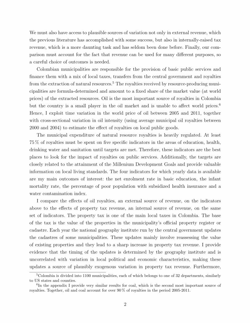
Colombian municipalities are responsible for the provision of basic public services and

finance them with a mix of local taxes, transfers from the central government and royalties

from the extraction of natural resources.5 The royalties received by resource-producing muni-

cipalities are formula-determined and amount to a fixed share of the market value (at world

prices) of the extracted resources. Oil is the most important source of royalties in Colombia

but the country is a small player in the oil market and is unable to affect world prices.6

Hence, I exploit time variation in the world price of oil between 2005 and 2011, together

with cross-sectional variation in oil intensity (using average municipal oil royalties between

2000 and 2004) to estimate the effect of royalties on local public goods.

The municipal expenditure of natural resource royalties is heavily regulated. At least

75 % of royalties must be spent on five specific indicators in the areas of education, health,

drinking water and sanitation until targets are met. Therefore, these indicators are the best

places to look for the impact of royalties on public services. Additionally, the targets are

closely related to the attainment of the Millenium Development Goals and provide valuable

information on local living standards. The four indicators for which yearly data is available

are my main outcomes of interest: the net enrolment rate in basic education, the infant

mortality rate, the percentage of poor population with subsidized health insurance and a

water contamination index.

I compare the effects of oil royalties, an external source of revenue, on the indicators

above to the effects of property tax revenue, an internal source of revenue, on the same

set of indicators. The property tax is one of the main local taxes in Colombia. The base

of the tax is the value of the properties in the municipality’s official property register or

cadastre. Each year the national geography institute run by the central government updates

the cadastres of some municipalities. These updates mainly involve reassessing the value

of existing properties and they lead to a sharp increase in property tax revenue. I provide

evidence that the timing of the updates is determined by the geography institute and is

uncorrelated with variation in local political and economic characteristics, making these

updates a source of plausibly exogenous variation in property tax revenue. Furthermore,

5Colombia is divided into 1100 municipalities, each of which belongs to one of 32 departments, similarlyto US states and counties.

6In the appendix I provide very similar results for coal, which is the second most important source ofroyalties. Together, oil and coal account for over 90 % of royalties in the period 2005-2011.

2

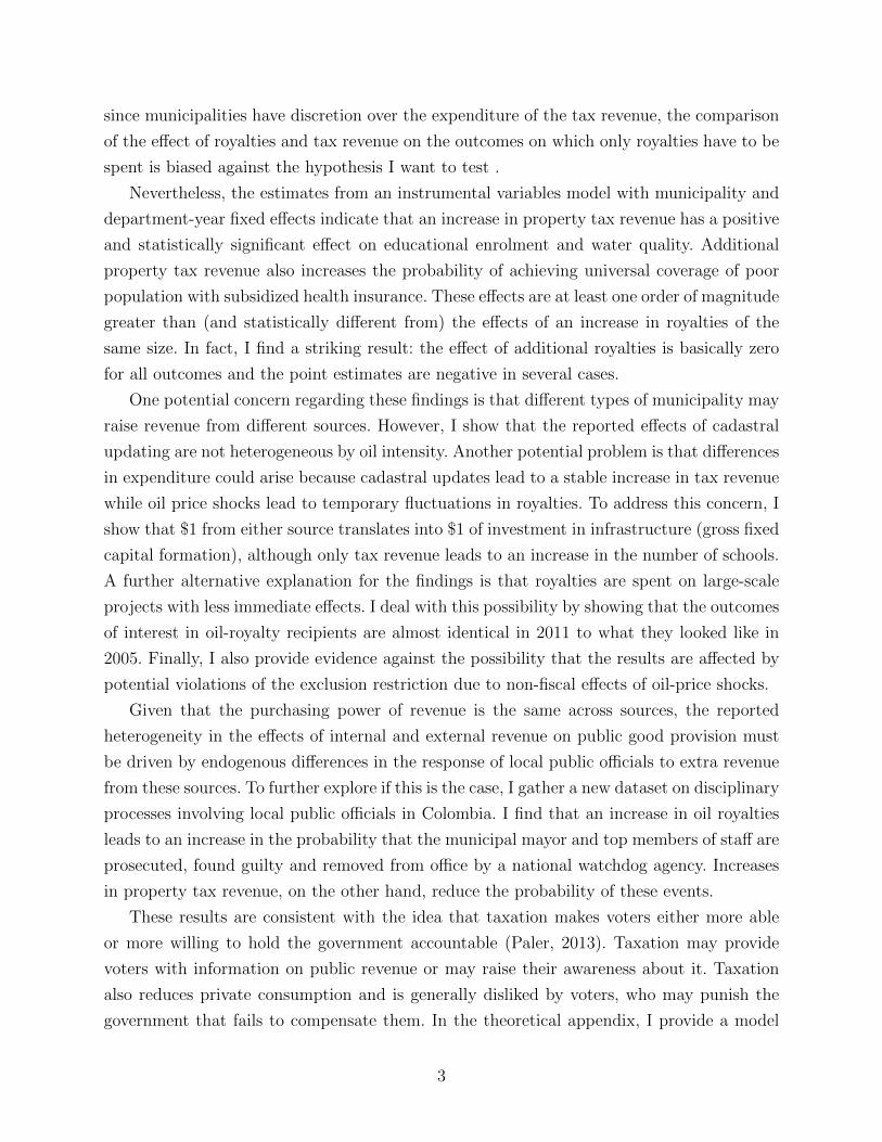
since municipalities have discretion over the expenditure of the tax revenue, the comparison

of the effect of royalties and tax revenue on the outcomes on which only royalties have to be

spent is biased against the hypothesis I want to test .

Nevertheless, the estimates from an instrumental variables model with municipality and

department-year fixed effects indicate that an increase in property tax revenue has a positive

and statistically significant effect on educational enrolment and water quality. Additional

property tax revenue also increases the probability of achieving universal coverage of poor

population with subsidized health insurance. These effects are at least one order of magnitude

greater than (and statistically different from) the effects of an increase in royalties of the

same size. In fact, I find a striking result: the effect of additional royalties is basically zero

for all outcomes and the point estimates are negative in several cases.

One potential concern regarding these findings is that different types of municipality may

raise revenue from different sources. However, I show that the reported effects of cadastral

updating are not heterogeneous by oil intensity. Another potential problem is that differences

in expenditure could arise because cadastral updates lead to a stable increase in tax revenue

while oil price shocks lead to temporary fluctuations in royalties. To address this concern, I

show that $1 from either source translates into $1 of investment in infrastructure (gross fixed

capital formation), although only tax revenue leads to an increase in the number of schools.

A further alternative explanation for the findings is that royalties are spent on large-scale

projects with less immediate effects. I deal with this possibility by showing that the outcomes

of interest in oil-royalty recipients are almost identical in 2011 to what they looked like in

2005. Finally, I also provide evidence against the possibility that the results are affected by

potential violations of the exclusion restriction due to non-fiscal effects of oil-price shocks.

Given that the purchasing power of revenue is the same across sources, the reported

heterogeneity in the effects of internal and external revenue on public good provision must

be driven by endogenous differences in the response of local public officials to extra revenue

from these sources. To further explore if this is the case, I gather a new dataset on disciplinary

processes involving local public officials in Colombia. I find that an increase in oil royalties

leads to an increase in the probability that the municipal mayor and top members of staff are

prosecuted, found guilty and removed from office by a national watchdog agency. Increases

in property tax revenue, on the other hand, reduce the probability of these events.

These results are consistent with the idea that taxation makes voters either more able

or more willing to hold the government accountable (Paler, 2013). Taxation may provide

voters with information on public revenue or may raise their awareness about it. Taxation

also reduces private consumption and is generally disliked by voters, who may punish the

government that fails to compensate them. In the theoretical appendix, I provide a model

3

of political agency with career concerns that illustrates how both information-based and

preference-based mechanisms can explain the results from the empirical exercise.

The present paper’s main contribution is to the empirical literature studying the rela-

tionship between public finance and governance.7 Within this literature, two recent papers

have studied the differential effects of internal and external revenue on public good provi-

sion, with mixed findings. Borge et al. (2015) show that additional rents from hydro-power

production reduce the efficiency of public expenditure less than increases in other revenue in

Norwegian municipalities. In the most closely related contribution to the present paper, Ga-

denne (2015) reports improvements in educational infrastructure for Brazilian municipalities

that enroll in a tax modernization program, while higher transfers have no effect.

The main challenge that this line of research still faces is coming up with plausibly

exogenous sources of variation in tax revenue, as changes in tax bases and tax rates are likely

to be endogenous to political and economic factors that can potentially affect outcomes of

interest. The present paper contributes to this literature by exploiting the quasi-random

timing of cadastral updates as a source of variation in internal revenue.8 These updates

lead to an increase in tax revenue that is not correlated to changes in political or economic

conditions, nor in tax administration or structure. I observe cadastral updates for 60 % of

municipalities in a five-year period, which ensures the representativeness of the results among

Colombian municipalities. It also allows me to show that the benefits of taxation extend to

the same municipalities where oil royalties have no effect. The present paper also contributes

to the existing literature by providing evidence on the heterogeneous effects of internal and

external revenue on politicians’ misconduct, based on novel data from disciplinary processes.

This paper is also related to to the empirical literature that uses sub-national data to

study the effects of natural resource rents.9 The theoretical model I develop also complements

previous contributions on the political resource curse by exploring the heterogeneous political

effects of resource rents relative to tax revenue.10 The paper contributes as well to the ‘second

7Zhuravskaya (2000) documents the negative effects of transfer offsets to increases in tax revenue inRussian cities. Ross (2004) reports cross-country evidence on the link between taxation and democracy.Paler (2013) and Martin (2014) provide experimental evidence on people’s higher willingness to hold thegovernment accountable when they are taxed. Borge and Rattsø (2008) and Sanchez and Pachon (2013)show that property taxes improve the efficiency and amount of public services in Norway and Colombia,respectively. Casaburi and Troiano (2015) report positive effects on local governance from the cadastralregistration of properties in Italy.

8Sanchez and Pachon (2013) use an IV strategy based on cadastral depreciation and find that educationalenrolment and water quality improve in Colombian municipalities that collect more taxes. I build on theirwork by providing the necessary evidence on the exogeneity of the timing of cadastral updates. Additionally,while Sanchez and Pachon (2013) study the effect of fiscal capacity on public good provision, I answer adifferent question related to the heterogeneous effects of internal and external revenue.

9See Caselli and Michaels (2013); Maldonado (2014); Ferraz and Monteiro (2014); Olsson and Valsecchi(2014); Herrera (2014); Carreri and Dube (2015).

10See Caselli (2006); Mehlum et al. (2006); Robinson et al. (2006); Caselli and Cunningham (2009); Brollo

4

generation’ literature on fiscal federalism by providing evidence on the importance of local

fiscal incentives.11

The rest of this paper is organized as follows. Section 2 presents the conceptual framework

behind the main hypothesis to be tested. Section 3 provides background information on the

setting for the empirical exercise. Section 4 presents the data and discusses the empirical

strategy. The main results are shown in section 5, leaving robustness checks and extensions

for section 6. Section 7 concludes.

2. Conceptual Framework

In this section I explore the reasons why we might expect internal and external revenue to

have heterogeneous effects on governance. One straightforward reason is because voters are

better informed about changes in taxation than about changes in external revenue. In the

theoretical appendix I explore this mechanism in the context of a political agency model with

career concerns.12 In the model, voters receive a noisy signal on public revenue, the precision

of which is improved by the share of taxes in total revenue. As the revenue signal becomes

more precise, voters are more able to infer the incumbent’s ability after observing public

good provision. Hence, taxation makes the voters’ posterior beliefs on the incumbent’s ability

more sensitive to observed public goods and this leads to higher effort by the incumbent and

more public goods. As external revenue increases, on the other hand, voters become less

well informed about revenue and this has a negative effect on the incumbent’s effort. Thus,

external revenue has a smaller effect on public goods than tax revenue.13

This informational explanation is consistent with various findings from the empirical li-

terature. Recent studies provide evidence in support of the idea that voters find it difficult

to establish the contribution of government to observed outcomes (Leigh, 2009; De la O,

2013; Guiteras and Mobarak, 2014). Recent research also indicates that voters are relati-

vely uninformed about changes in external revenue (Reinikka and Svensson, 2004; Ferraz

and Monteiro, 2014; Gadenne, 2015). Additionally, there is a large literature showing that

governments are generally more accountable to voters that are better informed.14

et al. (2013); Matsen et al. (2015)11See Bardhan (2002); Oates (2005); Bardhan and Mookherjee (2006); Faguet and Sanchez (2008, 2014);

Weingast (2009). Glaeser (1996) and Hoxby (1999) explore the potential of the property tax to act as adisciplining device for local governments.

12The model is an extension of the canonical career concerns model of Persson and Tabellini (2000) thatincorporates ‘signal-jamming’ a la Holmstrom (1999). Alesina and Tabellini (2007) and Matsen et al. (2015)use similar extensions to answer very different questions.

13Gadenne (2015) develops a similar model of moral hazard.14See Besley and Burgess (2002); Reinikka and Svensson (2005); Ferraz and Finan (2008); Bjorkman and

Svensson (2009); Snyder and Stromberg (2010); Banerjee et al. (2011); Fergusson et al. (2013); Chong et al.

5

One may still wonder how can residents of resource-rich areas not be aware of the flow

of resource rents to their government. The point here is that even if voters in these areas

know about the abundance of natural resource rents, they must still pay close attention to

fluctuations in prices and output to be well informed about the change in these rents. This

is important because both the model and the empirical exercise to follow are concerned with

changes in revenue from different sources, rather than with their average level.

One could also wonder how informative it is to pay your own taxes in a world with

significant heterogeneity in tax liabilities. Although this does raise the question about which

are the taxes that matter, it is not a major concern for the empirical exercise on Colombia as

the cadastral updates that I study lead to a municipality-wide simultaneous increase in tax

liabilities. A related question is whether increases to taxation simply make voters, who are

already well informed about revenue, more aware of the public purse and its use (increased

salience). An explanation along these lines seems particularly plausible because the property

tax that I study in the empirical exercise stands out in this respect, as it is a yearly out-

of-pocket tax payment on an illiquid asset (Cabral and Hoxby, 2015). Additionally, there is

evidence that people’s response to taxation is affected by the salience of taxes (Chetty et al.,

2009; Finkelstein, 2009).

There are, of course, other channels besides information and salience through which the

source of revenue may affect accountability and government performance. It is possible,

for instance, that voters simply dislike taxation and punish the incumbent for it unless he

compensates them with improved public services. Martin (2014) develops a model along

these lines in which loss-averse voters derive utility from punishing a corrupt government.15

In the appendix, I present an alternative version of the theoretical model described abo-

ve in which the marginal utility of public goods is decreasing in private consumption and

voters can acquire costly information on public revenue. I show that taxation may improve

incumbent effort and public good provision, even if it is not by itself directly informative,

because it induces the acquisition of costly information on government revenue due to its

negative effect on disposable income.

There is some empirical evidence supporting these preference-based channels. Both Paler

(2013) and Martin (2014) find that participants in lab experiments are more willing to engage

in costly punishment of a misbehaving government when the source of revenue is taxation

than when it is external, even when information is held constant across treatments. There is

also a large literature on reciprocity that has found that people are willing to incur in costly

(2015).15In my model, forward-looking voters cannot credibly commit to vote against the incumbent if they

believe him to be of higher ability than his opponent in the election.

6

punishment of what they consider to be unfair behavior (Fehr and Gachter, 2000).

Overall, taxation may either increase citizens’ willingness to hold the government ac-

countable or their ability to do so (Paler, 2013). Although the available data does not allow

me to distinguish between the explanations discussed above, all of them predict that tax

revenue has a larger effect on public good provision than external revenue. In the empirical

exercise that follows I provide empirical evidence in support of this hypothesis. Additional

evidence from disciplinary processes indicates that the actions of local governments respond

differently to increases in local taxation than to increases in external revenue.

3. Background

Following decentralization reform in the early 1990s, Colombian departments and muni-

cipalities became jointly responsible for the provision of basic public services in the areas of

education, health, drinking water and sanitation. The central government provides funding

for related expenditures through a system of earmarked and formula-determined transfers

called “Sistema General de Participaciones” (SGP). These transfers account on average for

63 % of a municipality’s total revenue and must be kept in a separate account from other

local revenues. Autonomy over the expenditure of transfers and over the administration of

public services varies across municipalities and across sectors, with the specific responsibili-

ties of the different levels of government for public service provision being somewhat blurry

(Alesina et al., 2005).16 However, as will become clear below, I verify that all municipalities

in the sample are legally able to use revenue from the two sources under study to improve

the outcomes of interest.

Taxes are the second most important source of municipal revenue after transfers and

contribute on average with 44 % of current receipts and 13 % of total revenue. The main local

taxes (and their average shares of tax revenue) are the property tax (34 %), the business tax

(17 %) and the petrol surcharge (22 %).17 The property tax is the most important source

of tax revenue for slightly more than one half of municipalities, but its relative importance

decreases with population size.18

16After an additional reform in 2001, municipalities “certified” by the Ministries of Education or Healthstarted to directly manage the transfers earmarked for these areas (Cortes, 2010; Brutti, 2015). Otherwise,transfers are managed by the departmental government. Certified municipalities also have greater autonomyin the management of the local education and health systems. However, the provision of health services ishighly regulated, even for certified municipalities, and must take place through special firms called “EmpresasSociales del Estado” (ESE). In the case of water and sanitation, municipalities manage the share of transfersearmarked for this purpose unless they are “de-certified” by the Superintendent for Public Services.

17Other local taxes include those for car registration and for the display of billboards and banners.18Glaeser (2013) reports that local public finances in the US are not very different, with intra-government

transfers and property taxes being the most important sources of revenue for all but the largest cities.

7

Municipalities have discretion over the expenditure of property tax revenue, except for

a fixed share that must be transferred to the corresponding environmental agency.19 All

municipalities can supply funding for the provision of education and they can also invest in

infrastructure and school equipment. In health, all municipalities are responsible for provi-

ding subsidized insurance to the population classified as poor by the national government’s

proxy-means-testing targeting system (SISBEN). Tax revenue can also be used for public

health initiatives such as vaccination campaigns (vaccines are provided at zero cost by the

central government). Regarding water and sanitation, municipalities can invest property tax

revenue in infrastructure or can also use it to provide subsidized access to these services to

the poor.

The property tax is levied on the cadastral value of all real estate in the municipality. The

cadastre or land register is the official record of the physical and economic characteristics

of all properties in a municipality. The three largest cities (Bogota, Medellın and Cali) as

well as the department of Antioquia have their own cadastral agencies and are excluded

from my sample. All others (86 % of municipalities) are under the authority of the National

geography institute, Instituto Geografico Agustın Codazzi (IGAC), an agency run by the

central government. IGAC periodically updates the cadastres under its control. This mainly

involves reassessing existing properties but also, to a much lesser extent, including in the

cadastre previously unregistered properties.20

The third most important source of local revenue are royalties from the extraction of

natural resources. Royalties are paid by firms to the central government according to a set

of fixed resource-specific formulae of the form

royalty = output × world price (USD) × exchange rate (COP/USD) × royalty rate

The vast majority of this revenue is then transferred to producing municipalities and de-

partments, as well as to the port municipalities from where resources are shipped, according

to predetermined shares. The main source of royalties is the extraction of oil. Oil royalties

amounted to 3.5 billion USD between 2005 and 2011, which accounts for 69 % of all royalties

paid in this period.21 18 % of municipalities received oil royalties and these represented, on

average, 23 % of total revenue.

Gadenne and Singhal (2014) show that dependence on external revenue is greater for local governments indeveloping countries.

19There are 34 such agencies in the country. Some cover a handful of municipalities while others covermultiple departments. The percentage transferred must be between 15 % and 25 % of property tax revenue.

20See Iregui et al. (2003, 2004) and Sanchez and Espana (2013) for further information on the propertytax in Colombia and on cadastral updating.

21Royalties are also paid for the extraction of coal, precious metals, gemstones, iron, copper, nickel andsalt.

8

By law, at least 75 % of royalties must be spent on education, health, drinking water

and sanitation until specific targets are met for the specific set of indicators listed in Table

1. These are the net enrolment rate in basic education (years 1-9, ages 6-14), the infant

mortality rate, the percentage of poor population with subsidized health insurance and the

percentages of population with access to drinking water and sanitation. Regarding water, it

is only considered suitable for human consumption (“drinkable”) if it scores less than 5 in

a water contamination index ranging from 0 to 100. Once all targets are met municipalities

keep receiving royalties and can spend them on priority projects from the mayor’s government

plan.

Royalties can be used to finance the provision of education if SGP transfers are shown to

be insufficient. Otherwise, royalties can be spent on education infrastructure, school equip-

ment or transportation. Royalty recipients can reduce infant mortality through public health

policies or by setting up emergency health posts for common infant diseases. Royalties can be

used for expenditures related to water and sewerage projects, such as initial studies, designs

and construction.

A reform in 2012 significantly reduced the royalties received by producing municipalities

and modified expenditure procedures. I drop years after 2011 from the sample for this reason,

but also due to some data limitations.

The top municipal authority is the mayor. Mayoral elections take place simultaneously in

all municipalities every four years. The local legislative body is the municipal council, which

varies in size with population and is elected at the same time as the mayor. The council

has to approve both the mayor’s general government plan and the annual budget and it is

responsible for monitoring their execution.

The watchdog agency Procuradurıa General de la Nacion (PGN) oversees public emplo-

yees’ compliance with the relevant disciplinary norms. This includes local public officials,

such as the mayor, top members of staff (e.g. secretary of education) and municipal council

members. PGN may start an investigation based on news reports, tip-offs, audit results and

reports from other government agencies such as the fiscal watchdog Contralorıa General de

la Republica (CGR). PGN can hand out sanctions ranging from fines and short suspensions

for small offences, to the removal from office and a ban from future public employment and

office. These latter sanctions are reserved for serious offences, such as intentional violations

of procurement, hiring and electoral laws.

9

4. Empirical Strategy

When voters are more aware or more affected by the way in which their local government

collects revenue, government accountability and public service provision improves. To test

this hypothesis, I use panel data for Colombian municipalities between 2005 and 2011 and

I compare the effects on local public good provision of shocks to local tax revenue to the

effects of changes in an external source of revenue, the royalties from the extraction of oil. I

exploit the timing of cadastral updates and fluctuations in the world price of oil as sources

of plausibly exogenous variation in property tax revenue and royalties, respectively. I further

test for heterogeneous effects of these sources of revenue on government performance by

looking at disciplinary processes involving local public officials.

I explain this empirical exercise in the following sub-sections. First, I introduce the data

employed. I then present the outcomes of interest. Finally, I discuss the identification strategy.

4.1. Data

The empirical exercise described above requires three main pieces of data. First, I need

data on the different sources of revenue of municipal governments. Second, I require informa-

tion on local public goods. Finally, I must also have information on the sources of variation

of both internal and external revenue. This means having data on cadastral updates, on the

world price of oil and on local oil abundance. All of these data must be available at the

municipality-year level to allow me to control for unobserved heterogeneity across municipa-

lities and over time.

Data on municipal public finance comes from the yearly balance sheets reported by each

municipality to the Office of the Comptroller General for the purpose of fiscal control. These

balance sheets have disaggregated information on all sources of revenue, including tax re-

venue (by type of tax), transfers and royalties. Information on expenditure is also available

in these balance sheets, disaggregated between current expenditure (operating costs) and

investment. I express all money values in millions of 2004 Colombian Pesos per capita (un-

less otherwise stated) using the Consumer Price Index and population estimates from the

National Statistical Agency (DANE).

Data on local public goods comes from various sources: the net enrollment rate in basic

education and the infant mortality rate are provided by the Ministry of Education and

DANE, respectively.22 The percentage of poor population with access to subsidized health

22The net enrolment rate is calculated by dividing the number of children with ages 6 to 14 enrolledin school years 1 to 9 by the number of children in this age group. Since data on enrolment and data onpopulation come from different sources, the resulting figure can actually exceed 100 %. I censor enrolmentrates above 100 % but the results are robust to using the original data.

10

insurance comes from the Ministry of Health.23 The water contamination index, Indice de

Riesgo de la Calidad del Agua (IRCA), has been calculated by the National Health Institute

since 2007. The other indicators are available since 2005. In the following section I explain

why I choose these indicators as the main outcomes of interest.

Regarding cadastral updating, IGAC has yearly data on the number of properties, the

cadastral value and the year of the last cadastral updates for both the urban and rural areas

of each municipality under its supervision. As mentioned above, the three largest cities in

the country (Bogota, Medellın and Cali) as well as the department of Antioquia have their

own cadastral agencies and are excluded from the analysis,so the final panel includes 969

municipalities (out of a total of 1123) between 2005 and 2011. In the empirical exercise I do

not distinguish between urban and rural updates, but the results are robust to the exclusion

of rural updates.

Data on oil royalties comes from the National oil company, Ecopetrol, for the period

2000-2003 and from the National Hydrocarbons Agency, Agencia Nacional de Hidrocarburos

(ANH), for the period 2004-2011. I use the average petroleum spot price from the IMF’s

International Financial Statistics (IFS).

The other main piece of information is a novel dataset on disciplinary processes involving

local public officials carried out by the Inspector General’s Office, Procuradurıa General de

la Nacion (PGN). I constructed the dataset using news reports from PGN’s website for the

years 2004-2015. For each process, I recorded the names of the accused, their roles in the

public administration, the nature of the charges, the timing of the events, the stage of the

process and the outcome. I collapse this data to the municipality-local political term level

(2001-2003, 2004-2007 and 2008-2011), since it is not always possible to pin down at the

yearly level the timing of the events for which officials are being accused.

Summary statistics for all variables employed in the paper are provided in Table 2.

4.2. Local Public Goods

As mentioned above, Colombian law stipulates that at least 75 % of royalties must be

spent on the improvement of basic public services until targets are met for a specific set of

indicators. The targets are displayed in column 1 of Table 1. I also show in column 2 the

average value for each indicator in 2005, the first year for which data is available, among oil-

royalty recipients. At the start of the sample, the average municipality receiving oil royalties

does not meet any of the targets. Column 3 provides further evidence on the low levels

of target achievement. It shows that, with the exception of access to drinking water, the

23Poor is defined as belonging to categories 1 or 2 of the Colombian proxy-means-testing system SISBEN.

11

percentage of oil-royalty recipients reaching each target is less than or equal to 30 % in all

cases.

The low levels of compliance imply that the targets were binding constraints during the

sample period and that royalties had to be spent on the improvement of the indicators in

Table 1. Administrative data on the expenditure of royalties, which is only available for

recent years, confirms that between 2010 and 2011 the average oil-royalty recipient spent

approximately 80 % of royalties on the attainment of the targets. Although municipalities

could potentially move revenue from other sources to other purposes as royalties increase,

I find that the ratio of royalties to own revenues among oil-royalty recipients averages 1.58

during the sample period. This means that even with full crowding-out of own investment

we can be sure that royalties are spent at the margin on meeting the targets.

Hence, the indicators in Table 1 are the best places to look for the impact of additional

royalties and I use them as the main outcomes of interest for the empirical exercise. Another

reason to focus on these indicators is because they are also a valuable source of information

on local living conditions and the targets are closely related to the attainment of some of the

United Nations’ Millenium Development Goals (MDG), such as achieving universal primary

education and reducing child mortality.

This choice of outcomes does introduce a bias in the comparison I carry out, since muni-

cipalities have discretion over tax revenue and are not required to spend it on the outcomes

of interest. The effect of royalties should be mechanically large, when compared to the effect

of tax revenue, due to the higher required propensity to spend revenue from royalties on the

studied outcomes. However, this bias works against the hypothesis that I want to test.

Yearly data between 2005 and 2011 is only available at the municipality level for four of

the indicators in Table 1: the net enrolment rate in basic education, the infant mortality rate,

the percentage of poor population with access to subsidized health insurance and, starting in

2007, the index of water contamination. Data on the percentages of population with access to

drinking water and sewerage is only available in the 2005 population census, so I leave these

two indicators out of the analysis. However, as mentioned above, access to drinking water is

a composite indicator that requires residents to have access to water and this water to be

suitable for human consumption, which is measured by the included water contamination

index. I verify that there is a strong cross-sectional correlation between the values of the

two omitted indicators in 2005 and the baseline score from 2007 in the water contamination

index.24 Additionally, Sanchez and Vega (2014) report a large positive effect of access to

drinking water on infant mortality, so this latter indicator could also capture improvements

24Sanchez and Pachon (2013) find a positive cross-sectional effect of local taxation on access to drinkingwater in 2005.

12

in access to water and sanitation.

4.3. Identification Strategy

I exploit the availability of yearly data on the outcomes of interest and on revenue from

different sources for each municipality to estimate a model with municipality and department-

year fixed effects. This allows me to control for unobservable persistent heterogeneity across

municipalities as well as for common shocks affecting all municipalities simultaneously, with

this effect being potentially heterogeneous across departments. I thus identify the effects of

revenue from the two sources on the outcomes of interest from within-municipality variation

over time, net of common within-department time effects.

Still, OLS estimates of the fixed effects model could be affected by reverse causality

or by omitted variable bias. For example, a municipality could collect more taxes because

educational enrolment has risen due to the implementation of some other policy. Similarly,

royalties could increase due to the discovery of oil, which is likely to have a direct effect on

the outcomes of interest. Hence, I search for plausibly exogenous variation in both sources

of revenue in order to be able to claim that the estimates capture causal effects.

I use the timing of cadastral updates by IGAC as a source of exogenous variation in

property tax revenue. Colombian law requires municipal cadastres to be updated every five

years, but this condition is rarely satisfied. During the sample period, the average urban

update takes place 11.4 years after the previous one, with this number being slightly lar-

ger (12.7) for rural updates. I address potential concerns about the endogenous timing of

cadastral updates in three ways.

First, I check that the timing of the update is not affected by observable municipal

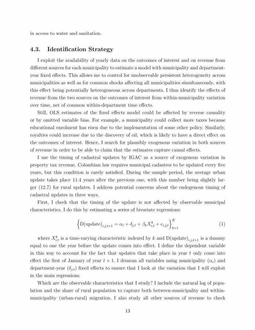
characteristics. I do this by estimating a series of bivariate regressions:{D(update)i,j,t+1 = αi + δj,t + βkX

ki,t + εi,j,t

}Kk=1

(1)

where Xki,t is a time-varying characteristic indexed by k and D(update)i,j,t+1 is a dummy

equal to one the year before the update comes into effect. I define the dependent variable

in this way to account for the fact that updates that take place in year t only come into

effect the first of January of year t + 1. I demean all variables using municipality (αi) and

department-year (δj,t) fixed effects to ensure that I look at the variation that I will exploit

in the main regressions.

Which are the observable characteristics that I study? I include the natural log of popu-

lation and the share of rural population to capture both between-municipality and within-

municipality (urban-rural) migration. I also study all other sources of revenue to check

13

whether updates try to offset or to complement other changes in revenue. I analyze poli-

tical competition, party affiliation and alignment across all levels of government: municipal

(mayor, council), departmental (governor) and national (president, congress). I look as well

at national policies, such as the number of families enrolled in the conditional cash-transfer

program Familias en Accion and the value of new loans made by the central government’s

agricultural bank. I check if cadastral updates are correlated with visits to the municipality

by President Alvaro Uribe because these visits led to significant policy commitments (Tribın,

2014). Finally, I look at indicators on crime, illegal armed group presence and cultivation

of narcotics. Although I am unable to rule out that variation in unobservables is affecting

the decision to update, it is not easy to think of changes in unobserved characteristics that

would not be picked up by the variables studied.

The results are presented in columns 1 and 2 of Table 3. Only the number of parties

participating in council elections, out of thirty variables considered, has a correlation with

the timing of cadastral updates that is statistically significant at the 10 % level.25 Although

this correlation could be spurious, I verify that results are robust to including any of the

variables considered as controls. I also show in the appendix that the results are robust

to the inclusion of municipality-term fixed effects, which capture any unobserved within-

municipality heterogeneity across local political terms. Furthermore, I check in columns 3

and 4 that the results are robust to adding separate dummies for the first five years after

urban and rural updates as controls. I ensure this way that the point estimates are not being

artificially attenuated by the fact that the probability of updating is essentially zero in the

years right after an update.

The second piece of evidence on the exogeneity of the cadastral updates is based on the

study of the supply of updates by IGAC. The sample period has the special feature that

IGAC received strong incentives to increase the number of updates. More specifically, Alvaro

Uribe included as part of his official government goals for his first term as President (2002-

2006) that IGAC should have the urban cadastres of all municipalities up to date (less than

five years old) by the end of the administration. For his second administration (2006-2010),

Uribe set as goals for IGAC to have 90 % of urban cadastres and 70 % of rural cadastres up

to date. Additionally, funding to IGAC increased, including an IDB loan for the purpose of

financing the cadastral updates of 145 municipalities in 2007.

Figure 1 shows the number of updated municipalities per year disaggregated by the type

of update. I indicate for each year who was President at the time, bearing in mind once

25Sanchez and Pachon (2013) and Sanchez and Espana (2013) report results from similar regressions usinga logit model. Although these authors find significant correlations with transfers, income and some politicalcharacteristics, the difference is probably driven by the lack of municipality fixed effects in those estimations.

14

again that there is a one-year lag in the validity of updated cadastres. The graph shows

that the number of updates increased sharply during the Uribe years: between 2006 and

2010, 60 % of municipalities have a cadastral update. This large number of updates coincides

with the positive supply shock caused by IGAC’s targets. Additional evidence that these

changes were driven by IGAC’s supply of updates comes from the fact that the share of

urban updates is high when the incentives are strong for urban updates (2004 to 2007) and

this share decreases when the incentives are strong for rural updates (after 2008). Figure 2

shows the percentage of properties up to date and confirms that the targets were binding

constraints for IGAC throughout the sample period.

I further use this variation in the supply of updates to look for evidence on selection into

cadastral updating. I consider the possibility that municipalities are intentionally updating

to collect more tax revenue and I try to get a sense of the size of this selection effect by

comparing the effect of updating on tax revenue across update cohorts. This exercise is

motivated by the large variation in number and type of updates shown in Figure 1, which

potentially reflects large differences in the composition of the update pool. The results, shown

in Figure 3, indicate that the returns to updating are fairly homogeneous across cohorts. I

am unable to reject the null hypothesis that the return is actually the same for all cohorts

between 2002 and 2011 at conventional levels of significance.

The final piece of evidence on the exogeneity of cadastral updates exploits IGAC’s yearly

planning of the updates. At the start of each year, IGAC drafts a list of municipalities to

be updated in that year, which the regional offices then use to negotiate with the municipal

and departmental governments regarding feasibility, funding and logistics. These lists are not

publicly available but I had access to the ones for 2011 and 2012. Matching these lists with the

actual updates that took place each year, I find that 80 % of updaters were in IGAC’s initial

list and 68 % of those pre-selected actually updated. Furthermore, results from regressions

using a specification similar to equation 1 reveal that the only robust predictors of inclusion

in the initial list are the number of years since the last urban and rural updates.

Taken together, the available evidence indicates that municipalities have a limited ability

to manipulate the timing of the cadastral updates and that this timing is mainly driven

by the supply from IGAC. However, municipalities have discretion over how much taxes to

collect. This autonomy over tax collection could be a problem if, for instance, only the mu-

nicipalities with good investment opportunities collect more taxes after a cadastral update.

Figure 3 already suggests that municipal governments do not enjoy large discretion over tax

collection. I provide evidence on statutory tax rates using data from Iregui et al. (2003) for

211 municipalities between 1999 and 2002. I regress the statutory property tax rate on a

dummy for the years after a cadastral update plus municipality and year fixed effects. The

15

results are shown in Table 4. The point estimates are very small and statistically insignifi-

cant, indicating that municipalities do not adjust statutory rates in response to cadastral

updates.26 Figure 4 further confirms that roughly 75 % of updaters between 2006 and 2010

experience an increase in property tax revenue following an update. The second part of the

identification strategy exploits plausibly exogenous variation in the world price of oil and the

heterogeneous distribution of this resource across municipalities. This type of difference-in-

differences methodology has been widely used in recent studies on Colombia.27 Identification

comes from the assumption that the world price of oil is exogenous to local conditions in

Colombian municipalities. This seems plausible, as Colombia is a relatively small exporter of

oil. According to the US Energy Information Administration, Colombia is the 18th largest

exporter of oil with less than 1 % of world exports.

I also assume that any systematic differences between municipalities with different levels

of oil abundance are time-invariant and thus captured by the municipality fixed effects.

As a measure of oil abundance I use the average amount of oil royalties received by the

municipality between 2000 and 2004 (royaltiesoili,00−04). Hence, what I exploit is the differential

impact of variation in the price of oil in municipalities with varying levels of oil extraction

in previous years (since royalties are a linear function of output). The variation from oil

discoveries, for example, is not exploited by this research design. Additionally, by using a

5-year average of previous oil royalties I address potential concerns about regression to the

mean.

Figure 7a summarizes the identification strategy for royalties. The black line shows the oil

price index I construct (2004=1). There is significant variation in oil prices during the sample

period: the price increases up to 2008, crashes in 2009 as a result of the global financial crisis

and recovers in the last two years. The figure also shows point estimates and 95 % confidence

intervals from a regression of the form

royaltiesi,j,t = αi + δj,t +2011∑

k=2006

βk [D(year = k)t ×D(oil royalties > 0)i,00−04] + εi,j,t (2)

where the dependent variable is royalties per capita in municipality i from department j

in year t. The coefficients of interest βk capture the average royalties among the set of

oil-rich municipalities (positive oil royalties between 2000 and 2004), net of municipality

and department-year fixed effects. The results in Figure 7a show that royalties in these

municipalities track the yearly variation in the price of oil.

26Sanchez and Espana (2013) provide additional evidence on the stickiness of statutory rates based oninterviews with public officials from several municipalities.

27See, for example, Dube and Vargas (2013); Carreri and Dube (2015); Santos (2014); Idrobo et al. (2014).

16

The map in Figure 5 shows sextiles of the distribution of (positive) average oil royalties

between 2000 and 2004. Two things stand out. First, although oil royalties are geographically

clustered in areas where there is oil, there is still substantial within-cluster variation in oil

intensity. The inclusion of department-year fixed effects ensures that I only exploit this

within-department variation in oil intensity. Second, a comparison with Figure 6 shows that

there is substantial overlap between oil-royalty recipients and municipalities with a cadastral

update. This allows me to verify that any differential effects across sources of revenue are

not driven by systematic differences in the use of revenue across municipalities, no matter

the source.

In what follows I use two main specifications. I show reduced-form effects of cadastral

updating and oil-price shocks using the following model:

yi,j,t = αi + δj,t + γTD(post-update)i,t + γR[priceoil

t × royaltiesoili,00−04

]+ εi,j,t (3)

where yi,j,t is an outcome of interest and αi and δj,t are municipality and department-year

fixed effects, respectively. The standard errors are clustered two-way by municipality and

department-year following Cameron et al. (2011). I standardize the “predicted” royalties

variable priceoilt × royaltiesoil

i,00−04 for ease of interpretation.

I estimate the effects of tax revenue and royalties on the outcomes of interest using an

instrumental variables model:

yi,j,t = αi + δj,t + βT property tax revenuei,t + βR natural resource royaltiesi,t + ui,j,t (4)

where the cadastral update dummy and the interaction of the oil price with oil intensity are

used as instruments for tax revenue and royalties, respectively.

To account for the fact that there may be a lag in the expenditure of royalties, I some-

times modify equations 3 and 4 and use cumulative royalties (∑t

k=2006 royaltiesi,k) instead

of contemporary values. The point here is that perhaps outcomes in year t are not so much

affected by royalties in that year but by the amount of royalties received in the previous

years. The municipality fixed effect absorbs all royalties up to 2005 and so these cumulatives

are partial ones since 2005. As an instrument for cumulative royalties I use the cumulative

of predicted royalties:∑t

k=2006 royaltiesoili,00−04 × priceoil

k .

Due to data constraints I change the unit of observation to municipality-local political

period for the regressions on disciplinary processes. I use data from the periods 2001-2003,

2004-2007 and 2008-2011. I use the oil royalties from 2000, supplied by Ecopetrol, as an

indicator of oil intensity.

17

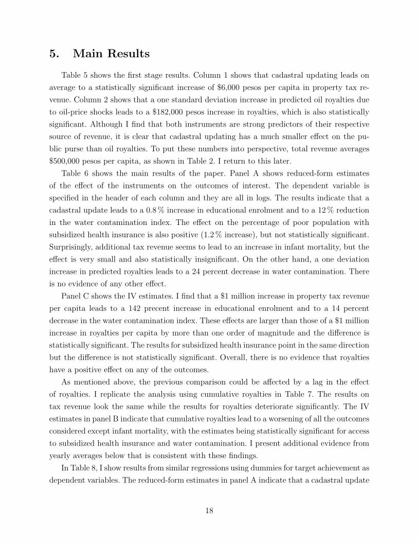
5. Main Results

Table 5 shows the first stage results. Column 1 shows that cadastral updating leads on

average to a statistically significant increase of $6,000 pesos per capita in property tax re-

venue. Column 2 shows that a one standard deviation increase in predicted oil royalties due

to oil-price shocks leads to a $182,000 pesos increase in royalties, which is also statistically

significant. Although I find that both instruments are strong predictors of their respective

source of revenue, it is clear that cadastral updating has a much smaller effect on the pu-

blic purse than oil royalties. To put these numbers into perspective, total revenue averages

$500,000 pesos per capita, as shown in Table 2. I return to this later.

Table 6 shows the main results of the paper. Panel A shows reduced-form estimates

of the effect of the instruments on the outcomes of interest. The dependent variable is

specified in the header of each column and they are all in logs. The results indicate that a

cadastral update leads to a 0.8 % increase in educational enrolment and to a 12 % reduction

in the water contamination index. The effect on the percentage of poor population with

subsidized health insurance is also positive (1.2 % increase), but not statistically significant.

Surprisingly, additional tax revenue seems to lead to an increase in infant mortality, but the

effect is very small and also statistically insignificant. On the other hand, a one deviation

increase in predicted royalties leads to a 24 percent decrease in water contamination. There

is no evidence of any other effect.

Panel C shows the IV estimates. I find that a $1 million increase in property tax revenue

per capita leads to a 142 precent increase in educational enrolment and to a 14 percent

decrease in the water contamination index. These effects are larger than those of a $1 million

increase in royalties per capita by more than one order of magnitude and the difference is

statistically significant. The results for subsidized health insurance point in the same direction

but the difference is not statistically significant. Overall, there is no evidence that royalties

have a positive effect on any of the outcomes.

As mentioned above, the previous comparison could be affected by a lag in the effect

of royalties. I replicate the analysis using cumulative royalties in Table 7. The results on

tax revenue look the same while the results for royalties deteriorate significantly. The IV

estimates in panel B indicate that cumulative royalties lead to a worsening of all the outcomes

considered except infant mortality, with the estimates being statistically significant for access

to subsidized health insurance and water contamination. I present additional evidence from

yearly averages below that is consistent with these findings.

In Table 8, I show results from similar regressions using dummies for target achievement as

dependent variables. The reduced-form estimates in panel A indicate that a cadastral update

18

increases the probability of having universal coverage of poor population with subsidized

health insurance by 3 percentage points. This is a relatively large effect, given that only

15 % of municipalities met this target in 2005, and it is also statistically significant at the

10 % level. Column 4 additionally shows that a cadastral update leads to an increase of 7.6

percentage points in the probability that water in the municipality is suitable for human

consumption. When scaled by revenue using the IV estimator, I find that these effects on

health and water are significantly different from those of additional royalties. None of the

point estimates for royalties in panel B are statistically different from zero. Results using

cumulative royalties, shown in Table 9, lead to similar conclusions.

I next verify that the previous results are coming from different sources of revenue rat-

her than from different sets of municipalities, cadastral updaters and oil-royalty recipients.

In Table 10 I explore the possibility of heterogeneity in the effects of cadastral updating

depending on oil abundance, defined in the same way as in the estimations above: average

oil royalties between 2000 and 2004. The results show no evidence of heterogeneity in the

effects of cadastral updating by oil intensity. The point estimates for the interaction between

cadastral updating and oil abundance are very small and never statistically different from

zero. Furthermore, I can reject the null that the effect of updating is zero on educational

enrolment, water contamination and health insurance affiliation for the median and mean

levels of oil intensity.

The previous results provide systematic evidence that increases in local tax revenue

resulting from cadastral updates lead to larger improvements in local public good provision

than oil-price driven increases in royalties of the same magnitude. I provide evidence that

these results are driven by a differential response from local governments to increases in

revenue from these two sources using the data on disciplinary processes.

Table 11 shows the results. The reduced-form estimates in panel A indicate that higher

oil prices lead to a worsening of local government performance in municipalities that are

oil-royalty recipients. A one standard deviation increase in predicted royalties increases the

probability that the local mayor is prosecuted (25 percentage points), found guilty (22 per-

centage points) and removed from office (14 percentage points). Similar results are found for

top members of staff. Cadastral updating, on the other hand, has a negative effect on the

likelihood of these events, though the estimates are statistically insignificant.

The IV estimates point in the same direction: increases in royalties increase the probabi-

lity of disciplinary processes involving local public officials while increases in royalties reduce

this probability. The findings in columns 3 and 6 are very telling, as they indicate that the

offenses committed by local public officials are serious ones such as embezzlement and co-

rruption. These results provide evidence in support of changes in incumbent performance as

19

the underlying mechanism for the observed difference across sources of revenue in the effects

on development indicators.

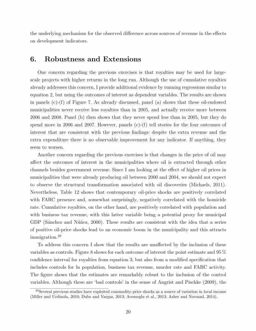
6. Robustness and Extensions

One concern regarding the previous exercises is that royalties may be used for large-

scale projects with higher returns in the long run. Although the use of cumulative royalties

already addresses this concern, I provide additional evidence by running regressions similar to

equation 2, but using the outcomes of interest as dependent variables. The results are shown

in panels (c)-(f) of Figure 7. As already discussed, panel (a) shows that these oil-endowed

municipalities never receive less royalties than in 2005, and actually receive more between

2006 and 2008. Panel (b) then shows that they never spend less than in 2005, but they do

spend more in 2006 and 2007. However, panels (c)-(f) tell stories for the four outcomes of

interest that are consistent with the previous findings: despite the extra revenue and the

extra expenditure there is no observable improvement for any indicator. If anything, they

seem to worsen.

Another concern regarding the previous exercises is that changes in the price of oil may

affect the outcomes of interest in the municipalities where oil is extracted through other

channels besides government revenue. Since I am looking at the effect of higher oil prices in

municipalities that were already producing oil between 2000 and 2004, we should not expect

to observe the structural transformation associated with oil discoveries (Michaels, 2011).

Nevertheless, Table 12 shows that contemporary oil-price shocks are positively correlated

with FARC presence and, somewhat surprisingly, negatively correlated with the homicide

rate. Cumulative royalties, on the other hand, are positively correlated with population and

with business tax revenue, with this latter variable being a potential proxy for municipal

GDP (Sanchez and Nunez, 2000). These results are consistent with the idea that a series

of positive oil-price shocks lead to an economic boom in the municipality and this attracts

immigration.28

To address this concern I show that the results are unaffected by the inclusion of these

variables as controls. Figure 8 shows for each outcome of interest the point estimate and 95 %

confidence interval for royalties from equation 3, but also from a modified specification that

includes controls for ln population, business tax revenue, murder rate and FARC activity.

The figure shows that the estimates are remarkably robust to the inclusion of the control

variables. Although these are ‘bad controls’ in the sense of Angrist and Pischke (2009), the

28Several previous studies have exploited commodity-price shocks as a source of variation in local income(Miller and Urdinola, 2010; Dube and Vargas, 2013; Acemoglu et al., 2013; Asher and Novosad, 2014).

20

robustness of the estimates on royalties to their inclusion indicates that these variables are

not mediating the estimated effects.

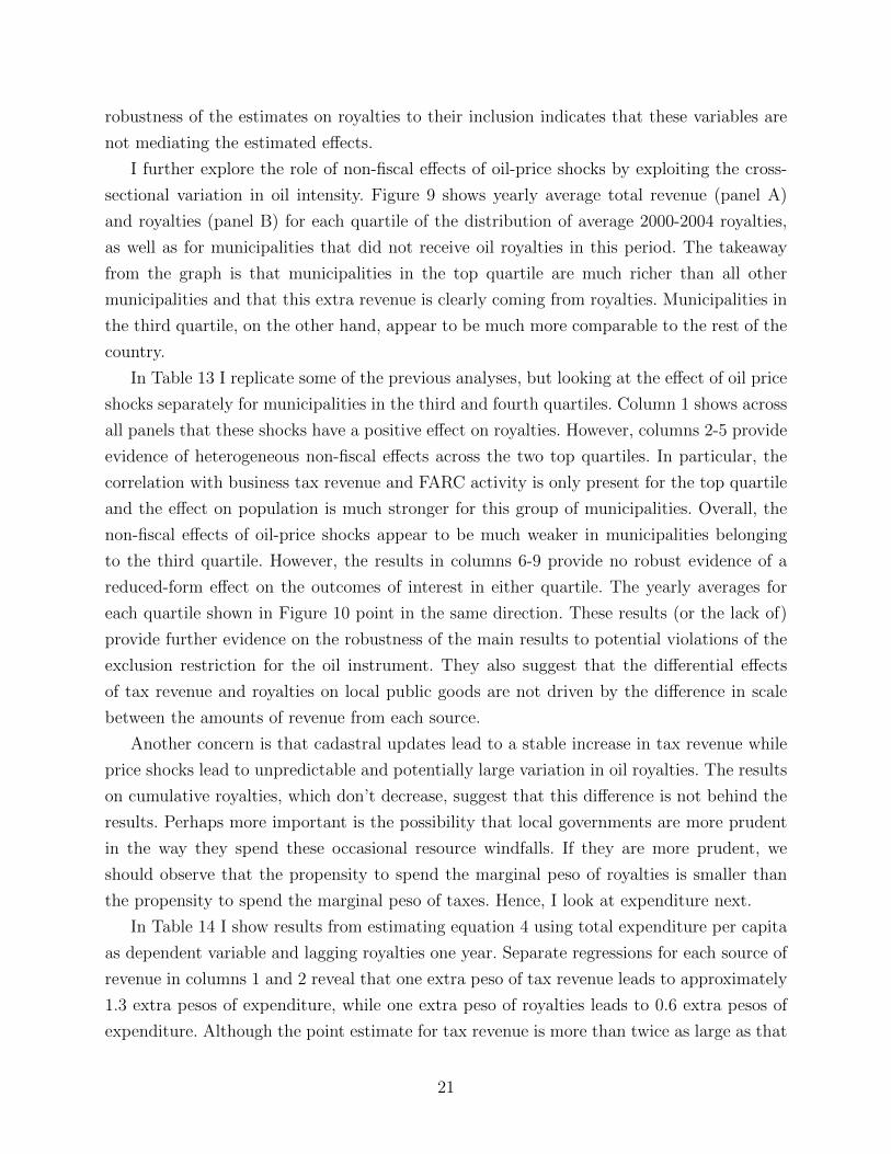
I further explore the role of non-fiscal effects of oil-price shocks by exploiting the cross-

sectional variation in oil intensity. Figure 9 shows yearly average total revenue (panel A)

and royalties (panel B) for each quartile of the distribution of average 2000-2004 royalties,

as well as for municipalities that did not receive oil royalties in this period. The takeaway

from the graph is that municipalities in the top quartile are much richer than all other

municipalities and that this extra revenue is clearly coming from royalties. Municipalities in

the third quartile, on the other hand, appear to be much more comparable to the rest of the

country.

In Table 13 I replicate some of the previous analyses, but looking at the effect of oil price

shocks separately for municipalities in the third and fourth quartiles. Column 1 shows across

all panels that these shocks have a positive effect on royalties. However, columns 2-5 provide

evidence of heterogeneous non-fiscal effects across the two top quartiles. In particular, the

correlation with business tax revenue and FARC activity is only present for the top quartile

and the effect on population is much stronger for this group of municipalities. Overall, the

non-fiscal effects of oil-price shocks appear to be much weaker in municipalities belonging

to the third quartile. However, the results in columns 6-9 provide no robust evidence of a

reduced-form effect on the outcomes of interest in either quartile. The yearly averages for

each quartile shown in Figure 10 point in the same direction. These results (or the lack of)

provide further evidence on the robustness of the main results to potential violations of the

exclusion restriction for the oil instrument. They also suggest that the differential effects

of tax revenue and royalties on local public goods are not driven by the difference in scale

between the amounts of revenue from each source.

Another concern is that cadastral updates lead to a stable increase in tax revenue while

price shocks lead to unpredictable and potentially large variation in oil royalties. The results

on cumulative royalties, which don’t decrease, suggest that this difference is not behind the

results. Perhaps more important is the possibility that local governments are more prudent

in the way they spend these occasional resource windfalls. If they are more prudent, we

should observe that the propensity to spend the marginal peso of royalties is smaller than

the propensity to spend the marginal peso of taxes. Hence, I look at expenditure next.

In Table 14 I show results from estimating equation 4 using total expenditure per capita

as dependent variable and lagging royalties one year. Separate regressions for each source of

revenue in columns 1 and 2 reveal that one extra peso of tax revenue leads to approximately

1.3 extra pesos of expenditure, while one extra peso of royalties leads to 0.6 extra pesos of

expenditure. Although the point estimate for tax revenue is more than twice as large as that

21

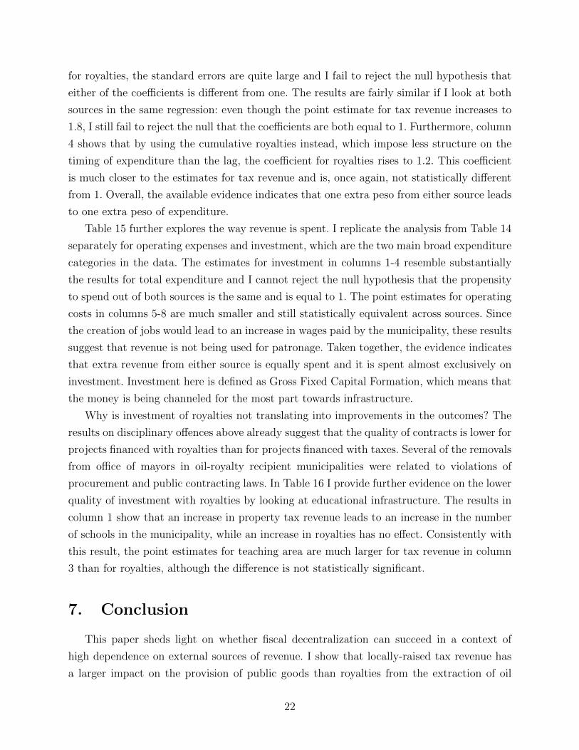
for royalties, the standard errors are quite large and I fail to reject the null hypothesis that

either of the coefficients is different from one. The results are fairly similar if I look at both

sources in the same regression: even though the point estimate for tax revenue increases to

1.8, I still fail to reject the null that the coefficients are both equal to 1. Furthermore, column

4 shows that by using the cumulative royalties instead, which impose less structure on the

timing of expenditure than the lag, the coefficient for royalties rises to 1.2. This coefficient

is much closer to the estimates for tax revenue and is, once again, not statistically different

from 1. Overall, the available evidence indicates that one extra peso from either source leads

to one extra peso of expenditure.

Table 15 further explores the way revenue is spent. I replicate the analysis from Table 14

separately for operating expenses and investment, which are the two main broad expenditure

categories in the data. The estimates for investment in columns 1-4 resemble substantially

the results for total expenditure and I cannot reject the null hypothesis that the propensity

to spend out of both sources is the same and is equal to 1. The point estimates for operating

costs in columns 5-8 are much smaller and still statistically equivalent across sources. Since

the creation of jobs would lead to an increase in wages paid by the municipality, these results

suggest that revenue is not being used for patronage. Taken together, the evidence indicates

that extra revenue from either source is equally spent and it is spent almost exclusively on

investment. Investment here is defined as Gross Fixed Capital Formation, which means that

the money is being channeled for the most part towards infrastructure.

Why is investment of royalties not translating into improvements in the outcomes? The

results on disciplinary offences above already suggest that the quality of contracts is lower for

projects financed with royalties than for projects financed with taxes. Several of the removals

from office of mayors in oil-royalty recipient municipalities were related to violations of

procurement and public contracting laws. In Table 16 I provide further evidence on the lower

quality of investment with royalties by looking at educational infrastructure. The results in

column 1 show that an increase in property tax revenue leads to an increase in the number

of schools in the municipality, while an increase in royalties has no effect. Consistently with

this result, the point estimates for teaching area are much larger for tax revenue in column

3 than for royalties, although the difference is not statistically significant.

7. Conclusion

This paper sheds light on whether fiscal decentralization can succeed in a context of

high dependence on external sources of revenue. I show that locally-raised tax revenue has

a larger impact on the provision of public goods than royalties from the extraction of oil

22

in Colombian municipalities. There is, in fact, no robust evidence of an effect of royalties

on public services over the period 2005-2011, despite the fact that royalties are earmarked

for this purpose. I complement these findings with evidence from disciplinary processes that

indicates that internal and external revenue have opposite effects on the misbehavior of local

public officials.

Where does the power of taxation lie? I am unable to distinguish between an explanation

based on information, where voters are better informed about tax revenue, and one based

on preferences, where voters dislike taxation. Future research must try to better understand

the relative importance of these two mechanisms, as this could determine what the optimal

policy to address the limitations of current decentralization schemes is. The experimental

work in Paler (2013) and Martin (2014) constitutes early steps in this direction, although it

would be desirable to obtain evidence from outside the lab on this matter. Another avenue

for future research is related to the study of different tax instruments with the objective of

establishing which characteristics (e.g. salience) are particularly important for accountability.

Nevertheless, these considerations are of second order relative to the fact that the return

to external revenue is much lower than that of tax revenue. The findings of this paper have

implications for important policy debates regarding fiscal federalism and the management of

natural resource wealth. They are also relevant for discussions on foreign aid. Overall, these

findings invite policymakers to reconsider the benefits from the disbursement of resources to

local governments without a locally-financed counterpart. They also suggest that investments

in local fiscal capacity may have much higher returns than previously expected.

References

Acemoglu, Daron, Amy Finkelstein, and Matthew J. Notowidigdo (2013), “Income and

health spending: Evidence from oil price shocks.” The Review of Economics and Statistics,

95 (4), 1079–1095.

Alesina, Alberto, Alberto Carrasquilla, and Juan Jose Echevarria (2005), “Decentralization

in Colombia.” In Institutional reforms in Colombia (Alberto Alesina, ed.), MIT Press,

Cambridge, MA.

Alesina, Alberto and Guido Tabellini (2007), “Bureaucrats or politicians? part I: A single

policy task.” American Economic Review, 97 (1), 169–179.

Angrist, Joshua D. and Jorn-Steffen Pischke (2009), Mostly Harmless Econometrics: an em-

piricist’s companion. Princeton University Press, Princeton, NJ.

23

Asher, Samuel and Paul Novosad (2014), “Digging for development: Mining booms and local

economic development in India.” Working Paper.

Banerjee, Abhijit, Selvan Kumar, Rohini Pande, and Felix Su (2011), “Do informed voters

make better choices? experimental evidence from urban India.” Working Paper.

Bardhan, Pranab (2002), “Decentralization of governance and development.” Journal of

Economic Perspectives, 16 (4), 185–205.

Bardhan, Pranab and Dilip Mookherjee (2006), “Decentralization, corruption and govern-

ment accountability: An overview.” In International Handbook on the economics of co-

rruption (Susan Rose-Ackerman, ed.), Edward Elgar.

Bauer, Peter (1972), Dissent on development. Harvard University Press, Cambridge (Mass.).

Beblawi, Hazem (1990), “The rentier state in the arab world.” In The Arab State (Giacomo

Luciani, ed.), University of California Press, Berkeley.

Besley, Timothy and Robin Burgess (2002), “The political economy of government respon-

siveness: Theory and evidence from India.” The Quarterly Journal of Economics, 117 (4),

1415–1451.

Besley, Timothy and Maitreesh Ghatak (2006), “Public goods and economic development.”

In Understanding Poverty (Abhijit Banerjee, Roland Benabou, and Dilip Mookherjee,

eds.), Oxford University Press.

Besley, Timothy and Torsten Persson (2011), Pillars of Prosperity: The Political Economics

of Development Clusters. Princeton University Press, Princeton, New Jersey.

Besley, Timothy and Torsten Persson (2013), “Taxation and development.” In Handbook of

public economics (Martin Feldstein Alan J. Auerbach, Raj Chetty and Emmanuel Saez,

eds.), volume 5, 51–110, Elsevier.

Besley, Timothy and Torsten Persson (2014), “Why do developing countries tax so little?”

Journal of Economic Perspectives, 28 (4), 99–120.

Bjorkman, Martina and Jakob Svensson (2009), “Power to the people: Evidence from a

randomized field experiment on community-based monitoring in Uganda.” The Quarterly

Journal of Economics, 124 (2), 735–769.

Borge, Lars-Erik, Pernille Parmer, and Ragnar Torvik (2015), “Local natural resource curse?”

Forthcoming, Journal of Public Economics.

24

Borge, Lars-Erik and Jørn Rattsø (2008), “Property taxation as incentive for cost control:

Empirical evidence for utility services in Norway.” European Economic Review, 52 (6),

1035–1054.

Brollo, Fernanda, Tommaso Nannicini, Roberto Perotti, and Guido Tabellini (2013), “The

political resource curse.” American Economic Review, 103 (5), 1759–1796.

Brutti, Zelda (2015), “Cities drifting apart: heterogeneous outcomes of decentralizing public

education.” Working Paper.

Cabral, Marika and Caroline Hoxby (2015), “The hated property tax: salience, tax rates and

tax revolts.” NBER Working Paper 18514.

Cameron, Colin, Jonah Gelbach, and Douglas Miller (2011), “Robust inference with multi-

way clustering.” Journal of Business and Economic Statistics, 29, 238–249.

Carreri, Maria and Oeindrila Dube (2015), “Do natural resources influence who comes to

power, and how?” Working Paper.

Casaburi, Lorenzo and Ugo Troiano (2015), “Ghost-house busters: The electoral response to

a large anti tax evasion program.” The Quarterly Journal of Economics, Forthcoming.

Caselli, Francesco (2006), “Power struggles and the natural resource curse.” Unpublished.

Caselli, Francesco and Tom Cunningham (2009), “Leader behaviour and the natural resource

curse.” Oxford Economic Papers, 61 (4), 628–650.

Caselli, Francesco and Guy Michaels (2013), “Do oil windfalls improve living standards?

evidence from Brazil.” American Economic Journal: Applied Economics, 5 (1), 208–38.

Chetty, Raj, Adam Looney, and Kory Kroft (2009), “Salience and taxation: Theory and

evidence.” American Economic Review, 99 (4), 1145–77.

Chong, Alberto, Ana De la O, Dean Karlan, and Leonard Wantchekon (2015), “Does co-

rruption information inspire the fight or quash the hope? a field experiment in Mexico on

voter turnout, choice and party identification.” The Journal of Politics, 77 (1), 55–71.

Collier, Paul (2006), “Is aid oil? an analysis of whether Africa can absorb more aid.” World

Development, 34 (9), 1482 – 1497.

Cortes, Darwin (2010), “Do more decentralized local governments do better? an evaluation

of the 2001 decentralization reform in Colombia.” Universidad del Rosario, Documento de

Trabajo 84.

25

De Janvry, Alain, Frederico Finan, and Elisabeth Sadoulet (2012), “Local electoral incentives

and decentralized program performance.” The Review of Economics and Statistics, 94 (3),

672–685.

De la O, Ana (2013), “Do conditional cash transfers affect electoral behavior? evidence from

a randomized experiment in Mexico.” American Journal of Political Science, 57 (1), 1–14.

Dewatripont, Mathias, Ian Jewitt, and Jean Tirole (1999), “The economics of career concerns,

part I: comparing information structures.” Review of Economic Studies, 66 (1), 183–198.

Dollery, Brian E. and Andrew C. Worthington (1996), “The empirical analysis of fiscal

illusion.” Journal of Economic Surveys, 10 (3), 261–297.

Dube, Oeindrila and Juan F. Vargas (2013), “Commodity price shocks and civil conflict:

Evidence from Colombia.” Review of Economic Studies, 80 (4), 1384–1421.

Easterly, William (2006), The white man’s burden: Why the West’s efforts to aid the rest

have done so much ill and so little good. Penguin, New York City.

Faguet, Jean-Paul (2014), “Decentralization and governance.” World Development, 53, 2–13.

Faguet, Jean-Paul and Fabio Sanchez (2008), “Decentralization’s effects on educational out-

comes in Bolivia and Colombia.” World Development, 36 (7), 1294–1316.

Faguet, Jean-Paul and Fabio Sanchez (2014), “Decentralization and access to social services

in Colombia.” Public Choice, 160 (1-2), 227–249.

Fehr, Ernst and Simon Gachter (2000), “Fairness and retaliation: The economics of recipro-

city.” Journal of Economic Perspectives, 14 (3), 159–181.

Fergusson, Leopoldo, Juan F. Vargas, and Mauricio Vela (2013), “Sunlight disinfects? free

media in weak democracies.” Documento CEDE 2013-14.

Ferraz, Claudio and Frederico Finan (2008), “Exposing corrupt politicians: The effects of

Brazil’s publicly released audits on electoral outcomes.” The Quarterly Journal of Econo-

mics, 123 (2), 703–745.

Ferraz, Claudio and Frederico Finan (2011), “Electoral accountability and corruption: Evi-

dence from the audits of local governments.” American Economic Review, 101 (4), 1274–

1311.

Ferraz, Claudio and Joana Monteiro (2014), “Learning to punish: Resource windfalls and

political accountability in Brazil.” Working Paper.

26

Finkelstein, Amy (2009), “E-ztax: Tax salience and tax rates.” The Quarterly Journal of

Economics, 124 (3), 969–1010.

Fisman, Raymond and Roberta Gatti (2002), “Decentralization and corruption: Evidence

from U.S. federal transfer programs.” Public Choice, 113 (1-2), 25–35.

Fujiwara, Thomas (2015), “Voting technology, political responsiveness, and infant health:

Evidence from Brazil.” Econometrica, 83 (2), 423–464.

Gadenne, Lucie (2015), “Tax me but spend wisely: Sources of public finance and government

accountability.” Working Paper.

Gadenne, Lucie and Monica Singhal (2014), “Decentralization in developing economies.”

Annual Review of Economics, 6 (1), 581–604.

Glaeser, Edward L. (1996), “The incentive effects of property taxes on local governments.”

Public Choice, 89 (1/2), 93–111.

Glaeser, Edward L. (2013), “Urban public finance.” In Handbook of public economics (Mar-

tin Feldstein Alan J. Auerbach, Raj Chetty and Emmanuel Saez, eds.), volume 5, 195–256,

Elsevier.

Guiteras, Raymond and Ahmed Mushfiq Mobarak (2014), “Does development aid undermine

political accountability? leader and constituent responses to a large-scale intervention.”

Working Paper.

Herrera, Juan Camilo (2014), “Petroleo y desarrollo: Efectos en la acumulacion y destruccion

de capital humano de los municipios de Colombia.” Documento CEDE, 2014 (10).

Holmstrom, Bengt (1999), “Managerial incentive problems: A dynamic perspective.” Review

of Economic Studies, 66 (1), 169–182.

Hoxby, Caroline (1999), “The productivity of schools and other local public goods produ-

cers.” Journal of Public Economics, 74 (1), 1–30.

Idrobo, Nicolas, Daniel Mejıa, and Ana Marıa Tribın (2014), “Illegal gold mining and violence

in Colombia.” Peace Economics, 20 (1), 83–111.

Iregui, Ana Marıa, Ligia Melo, and Jorge Ramos (2003), “El impuesto predial en Colombia:

evolucion reciente, comportamiento de las tarifas y potencial de recaudo.” Borradores de

Economıa 274, Banco de la Republica.

27

Iregui, Ana Marıa, Ligia Melo, and Jorge Ramos (2004), “El impuesto predial en Colombia:

Factores explicativos del recaudo.” Borradores de Economıa 319, Banco de la Republica.

Leigh, Andrew (2009), “Does the world economy swing national elections?” Oxford Bulletin

of Economics and Statistics, 71 (2), 163–181.

Litschig, Stephan and Kevin M. Morrison (2013), “The impact of intergovernmental trans-

fers on education outcomes and poverty reduction.” American Economic Journal: Applied

Economics, 5 (4), 206–40.

Mahdavy, Hossein (1970), “The patterns and problems of economic development in rentier

states: The case of Iran.” In Studies in the Economic History of the Middle East from the

Rise of Islam to the present day (M.A. Cook, ed.), Oxford University Press, London.

Maldonado, Stanislao (2014), “The political effects of resource booms: Political outcomes,

clientelism and public goods provision in Peru.” Working Paper.

Martin, Lucy (2014), “Taxation, loss aversion and accountability: Theory and experimental

evidence for taxation’s effect on citizen behavior.” Working Paper.

Martınez-Bravo, Monica, Gerard Padro i Miquel, Nancy Qian, and Yang Yao (2014), “Poli-

tical reform in China: the effect of local elections.” Working Paper.

Matsen, Egil, Gisle Natvik, and Ragnar Torvik (2015), “Petro Populism.” Forthcoming,

Journal of Development Economics.

Mehlum, Halvor, Karl Moene, and Ragnar Torvik (2006), “Institutions and the resource

curse.” The Economic Journal, 116 (508), 1–20.

Michaels, Guy (2011), “The long term consequences of resource-based specialisation.” The

Economic Journal, 121 (551), 31–57.

Miller, Grant and B. Piedad Urdinola (2010), “Cyclicality, mortality, and the value of time:

The case of coffee price fluctuations and child survival in Colombia.” Journal of Political

Economy, 118 (1), 113–155.

Mookherjee, Dilip (2015), “Political decentralization.” Annual Review of Economics, 7 (1),

231–249.

North, Douglass C. and Barry R. Weingast (1989), “Constitutions and commitment: The

evolution of institutional governing public choice in seventeenth-century England.” The

Journal of Economic History, 49 (4), 803–832.

28

Oates, Wallace (2005), “Toward a second-generation theory of fiscal federalism.” Internatio-

nal Tax and Public Finance, 12, 349–373.

Olsson, Ola and Michele Valsecchi (2014), “Resource windfalls and public goods: Evidence

from a policy reform in indonesia.” Working Paper.

Paler, Laura (2013), “Keeping the public purse: An experiment in windfalls, taxes, and the

incentives to restrain government.” American Political Science Review, 107 (4), 706–725.

Persson, Torsten and Guido Tabellini (2000), Political Economics: Explaining Economic

Policy. MIT Press, Cambridge (Mass.).

Pritchett, Lant and Yamini Aiyar (2014), “Value subtraction in public sector production:

Accounting versus economic cost of primary schooling in India.” Center for Global Deve-

lopment Working Paper, 2014 (391).

Reinikka, Ritva and Jakob Svensson (2004), “Local capture: Evidence from a central go-

vernment transfer program in Uganda.” The Quarterly Journal of Economics, 119 (2),

679–705.

Reinikka, Ritva and Jakob Svensson (2005), “Fighting corruption to improve schooling: Evi-

dence from a newspaper campaign in Uganda.” Journal of the European Economic Asso-

ciation, 3 (2-3), 259–267.

Robinson, James A., Ragnar Torvik, and Thierry Verdier (2006), “Political foundations of

the resource curse.” Journal of Development Economics, 79 (2), 447–468.

Ross, Michael L. (2001), “Does oil hinder democracy?” World Politics, 53, 325–361.

Ross, Michael L. (2004), “Does taxation lead to representation?” British Journal of Political

Science, 34 (2), 229–249.

Santos, Rafael (2014), “Not all that glitters is gold: Gold boom, child labor and schooling in

colombia.” Documento CEDE, 2014 (31).

Snyder, James M. and David Stromberg (2010), “Press coverage and political accountability.”

Journal of Political Economy, 118 (2), 355–408.

Sanchez, Fabio and Irina Espana (2013), “Estructura, potencial y desafıos del impuesto

predial en Colombia.” Documento CEDE, 2013 (48).

Sanchez, Fabio and Jairo Nunez (2000), “La geografıa y el desarrollo economico: Una apro-

ximacion municipal.” Desarrollo y Sociedad, 46, 43–108.

29

Sanchez, Fabio and Monica Pachon (2013), “Descentralizacion, esfuerzo fiscal y progreso

social en Colombia en el nivel local, 1994-2009: ¿por que importa la polıtica nacional?”

Documento CEDE, 2013 (38).

Sanchez, Fabio and Alexander Vega (2014), “Cobertura de acueducto y alcantarillado, ca-

lidad del agua y mortalidad infantil en Colombia, 2000-2012.” Documento CEDE, 2014

(40).

Tribın, Ana Marıa (2014), “Chasing votes with the public budget.” Working Paper.

Vicente, Pedro C. (2010), “Does oil corrupt? evidence from a natural experiment in West

Africa.” Journal of Development Economics, 92 (1), 28–38.

Weingast, Barry R. (2009), “Second generation fiscal federalism: The implications of fiscal

incentives.” Journal of Urban Economics, 65 (3), 279–293.

World Bank (2000), World Development Report 1999/2000: Entering the 21st century. Ox-

ford University Press.

World Bank (2004), World Development Report 2004: Making services work for poor people.

The World Bank and Oxford University Press.

Zhuravskaya, Ekaterina V. (2000), “Incentives to provide local public goods: fiscal federalism,

russian style.” Journal of Public Economics, 76 (3), 337–368.

30

Figure 1: Cadastral updates per year and presidential term

Note: I assign to each administration its first full calendar year (since presidential terms always start on August 7th) and thethree following ones. Each term is then pushed back by one year to account for the fact that updated cadastres only come intoeffect the 1st of January of the following year.

Figure 2: Percentage of properties with up-to-date cadastres

31

Figure 3: Property tax revenue increases after a cadastral update by cohort

The graph shows point estimates and 95 % confidence intervals for a regression of ln property tax revenue per capita (2004COP) on a set of dummies equal to one from year t onward if the municipality has a cadastral update on year t, weighted bythe share of the cadastre that was updated (depending on whether the update was urban, rural or both). I use property valuesfrom 2000 to determine the shares. The regression includes municipality and department-year fixed effects. Standard errorsclustered two-way by municipality and department-year.

Figure 4: Change in property tax revenue after a cadastral update

The graph shows the histogram for the difference between the average property tax revenue collected after a cadastral updateand the amount for the year before the update. Top and bottom 1 % removed for ease of visualization. Property tax revenue in2004 COP per capita. Update cohorts from 2006 to 2010. Pre-year corresponds to the first one in the case of multiple updates.

32

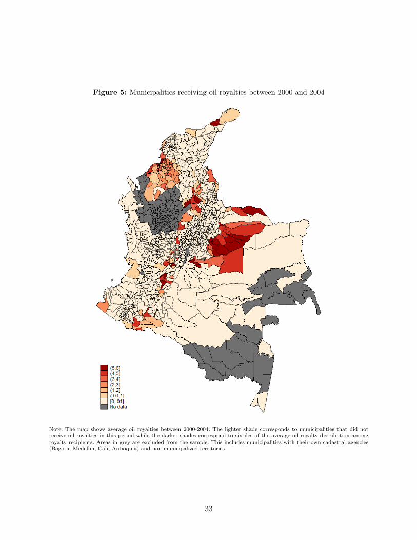
Figure 5: Municipalities receiving oil royalties between 2000 and 2004

Note: The map shows average oil royalties between 2000-2004. The lighter shade corresponds to municipalities that did notreceive oil royalties in this period while the darker shades correspond to sixtiles of the average oil-royalty distribution amongroyalty recipients. Areas in grey are excluded from the sample. This includes municipalities with their own cadastral agencies(Bogota, Medellin, Cali, Antioquia) and non-municipalized territories.

33

Figure 6: Municipalities with cadastral update (2006-2010)

Note: The map shows the location of municipalities that updated some portion of their cadastre between 2006 and 2010.Areasin grey are excluded from the sample. This includes municipalities with their own cadastral agencies (Bogota, Medellin, Cali,Antioquia) and non-municipalized territories.

34

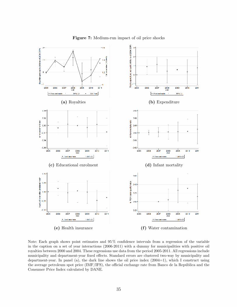
Figure 7: Medium-run impact of oil price shocks

(a) Royalties (b) Expenditure

(c) Educational enrolment (d) Infant mortality

(e) Health insurance (f) Water contamination

Note: Each graph shows point estimates and 95 % confidence intervals from a regression of the variablein the caption on a set of year interactions (2006-2011) with a dummy for municipalities with positive oilroyalties between 2000 and 2004. These regressions use data from the period 2005-2011. All regressions includemunicipality and department-year fixed effects. Standard errors are clustered two-way by municipality anddepartment-year. In panel (a), the dark line shows the oil price index (2004=1), which I construct usingthe average petroleum spot price (IMF/IFS), the official exchange rate from Banco de la Republica and theConsumer Price Index calculated by DANE.

35

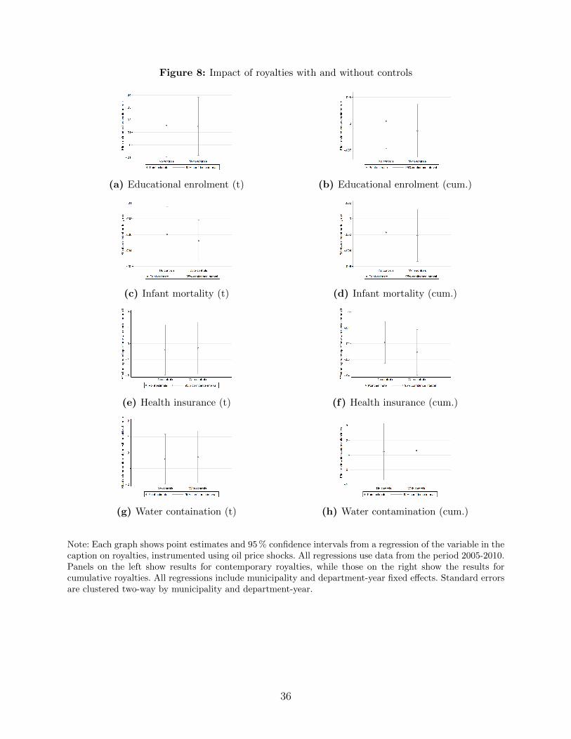
Figure 8: Impact of royalties with and without controls

(a) Educational enrolment (t) (b) Educational enrolment (cum.)

(c) Infant mortality (t) (d) Infant mortality (cum.)

(e) Health insurance (t) (f) Health insurance (cum.)

(g) Water containation (t) (h) Water contamination (cum.)

Note: Each graph shows point estimates and 95 % confidence intervals from a regression of the variable in thecaption on royalties, instrumented using oil price shocks. All regressions use data from the period 2005-2010.Panels on the left show results for contemporary royalties, while those on the right show the results forcumulative royalties. All regressions include municipality and department-year fixed effects. Standard errorsare clustered two-way by municipality and department-year.

36

Figure 9: Total revenue and royalties by average 2000-2004 oil royalties

Note: The figures show average total revenue (panel A) and avearge royalties (panel B) for each quartileof the average 2000-2004 positive oil royalties distribution. It also shows this information for municipalitieswith no oil royalties between 2000 and 2004. All money values in millions of 2004 COP per capita.

37

Figure 10: Medium-run impact of oil price shocks for the top two quartiles of oil abundance

(a) Royalties (b) Expenditure

(c) Educational enrolment (d) Infant mortality

(e) Health insurance (f) Water contamination

Note: Each graph shows point estimates and 95 % confidence intervals from a regression of the variablein the caption on a set of year interactions (2006-2011) with a dummy for municipalities with positive oilroyalties between 2000 and 2004. These regressions use data from the period 2005-2011. All regressions includemunicipality and department-year fixed effects. Standard errors are clustered two-way by municipality anddepartment-year. In panel (a), the dark line shows the oil price index (2004=1), which I construct usingthe average petroleum spot price (IMF/IFS), the official exchange rate from Banco de la Republica and theConsumer Price Index calculated by DANE.

38

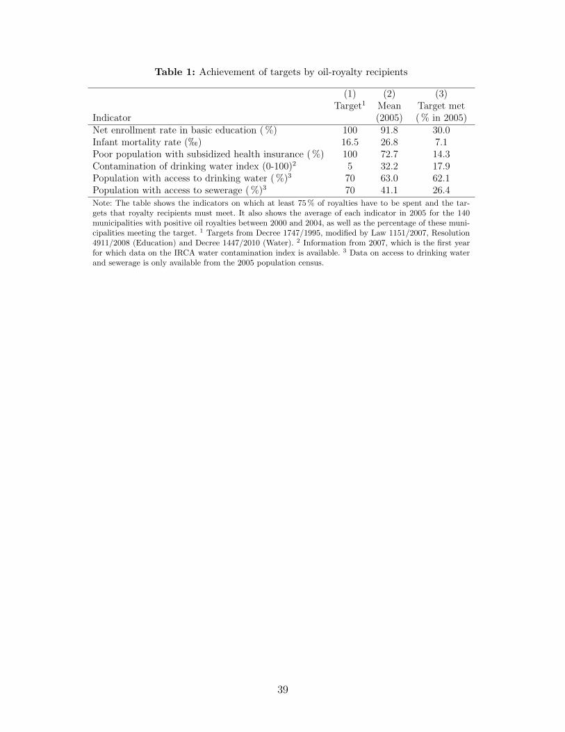
Table 1: Achievement of targets by oil-royalty recipients

(1) (2) (3)Target1 Mean Target met

Indicator (2005) ( % in 2005)Net enrollment rate in basic education ( %) 100 91.8 30.0Infant mortality rate (h) 16.5 26.8 7.1Poor population with subsidized health insurance ( %) 100 72.7 14.3Contamination of drinking water index (0-100)2 5 32.2 17.9Population with access to drinking water ( %)3 70 63.0 62.1Population with access to sewerage ( %)3 70 41.1 26.4Note: The table shows the indicators on which at least 75 % of royalties have to be spent and the tar-gets that royalty recipients must meet. It also shows the average of each indicator in 2005 for the 140municipalities with positive oil royalties between 2000 and 2004, as well as the percentage of these muni-cipalities meeting the target. 1 Targets from Decree 1747/1995, modified by Law 1151/2007, Resolution4911/2008 (Education) and Decree 1447/2010 (Water). 2 Information from 2007, which is the first yearfor which data on the IRCA water contamination index is available. 3 Data on access to drinking waterand sewerage is only available from the 2005 population census.

39

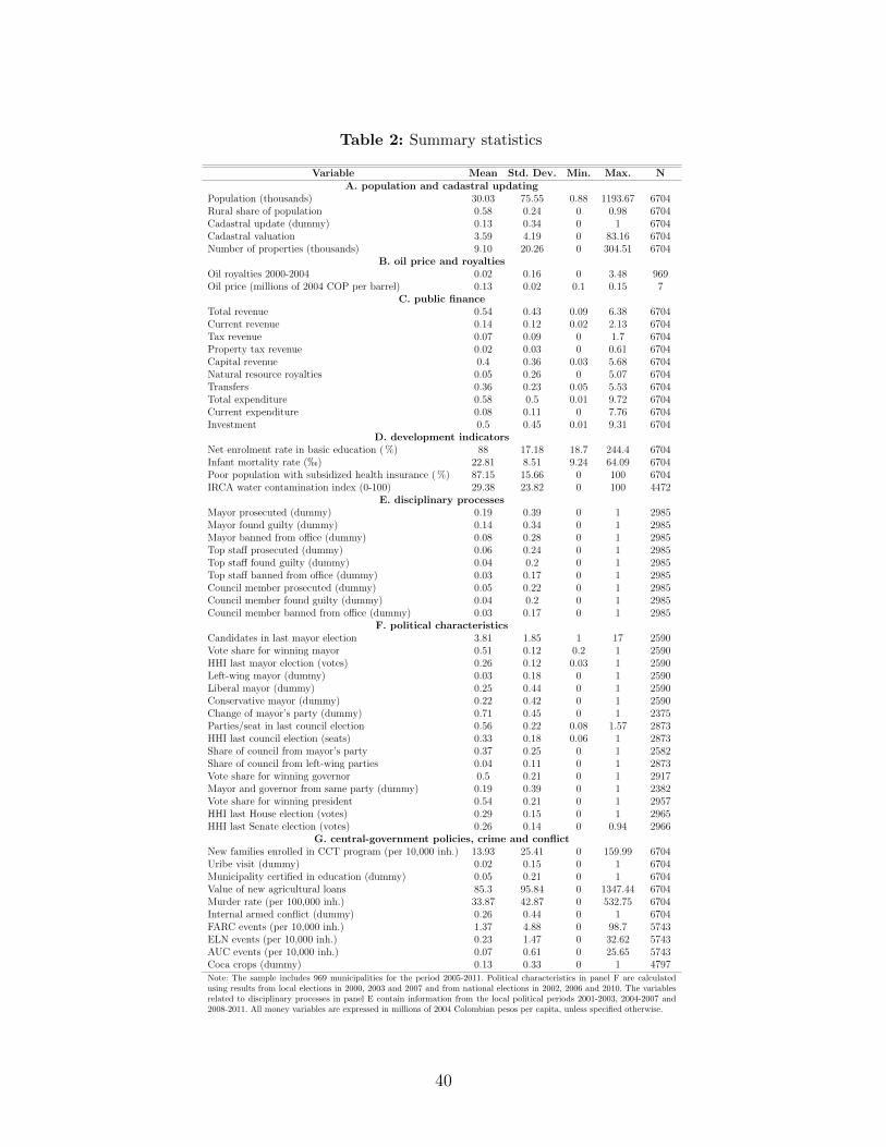
Table 2: Summary statistics

Variable Mean Std. Dev. Min. Max. NA. population and cadastral updating

Population (thousands) 30.03 75.55 0.88 1193.67 6704Rural share of population 0.58 0.24 0 0.98 6704Cadastral update (dummy) 0.13 0.34 0 1 6704Cadastral valuation 3.59 4.19 0 83.16 6704Number of properties (thousands) 9.10 20.26 0 304.51 6704

B. oil price and royaltiesOil royalties 2000-2004 0.02 0.16 0 3.48 969Oil price (millions of 2004 COP per barrel) 0.13 0.02 0.1 0.15 7

C. public financeTotal revenue 0.54 0.43 0.09 6.38 6704Current revenue 0.14 0.12 0.02 2.13 6704Tax revenue 0.07 0.09 0 1.7 6704Property tax revenue 0.02 0.03 0 0.61 6704Capital revenue 0.4 0.36 0.03 5.68 6704Natural resource royalties 0.05 0.26 0 5.07 6704Transfers 0.36 0.23 0.05 5.53 6704Total expenditure 0.58 0.5 0.01 9.72 6704Current expenditure 0.08 0.11 0 7.76 6704Investment 0.5 0.45 0.01 9.31 6704

D. development indicatorsNet enrolment rate in basic education ( %) 88 17.18 18.7 244.4 6704Infant mortality rate (h) 22.81 8.51 9.24 64.09 6704Poor population with subsidized health insurance ( %) 87.15 15.66 0 100 6704IRCA water contamination index (0-100) 29.38 23.82 0 100 4472

E. disciplinary processesMayor prosecuted (dummy) 0.19 0.39 0 1 2985Mayor found guilty (dummy) 0.14 0.34 0 1 2985Mayor banned from office (dummy) 0.08 0.28 0 1 2985Top staff prosecuted (dummy) 0.06 0.24 0 1 2985Top staff found guilty (dummy) 0.04 0.2 0 1 2985Top staff banned from office (dummy) 0.03 0.17 0 1 2985Council member prosecuted (dummy) 0.05 0.22 0 1 2985Council member found guilty (dummy) 0.04 0.2 0 1 2985Council member banned from office (dummy) 0.03 0.17 0 1 2985

F. political characteristicsCandidates in last mayor election 3.81 1.85 1 17 2590Vote share for winning mayor 0.51 0.12 0.2 1 2590HHI last mayor election (votes) 0.26 0.12 0.03 1 2590Left-wing mayor (dummy) 0.03 0.18 0 1 2590Liberal mayor (dummy) 0.25 0.44 0 1 2590Conservative mayor (dummy) 0.22 0.42 0 1 2590Change of mayor’s party (dummy) 0.71 0.45 0 1 2375Parties/seat in last council election 0.56 0.22 0.08 1.57 2873HHI last council election (seats) 0.33 0.18 0.06 1 2873Share of council from mayor’s party 0.37 0.25 0 1 2582Share of council from left-wing parties 0.04 0.11 0 1 2873Vote share for winning governor 0.5 0.21 0 1 2917Mayor and governor from same party (dummy) 0.19 0.39 0 1 2382Vote share for winning president 0.54 0.21 0 1 2957HHI last House election (votes) 0.29 0.15 0 1 2965HHI last Senate election (votes) 0.26 0.14 0 0.94 2966

G. central-government policies, crime and conflictNew families enrolled in CCT program (per 10,000 inh.) 13.93 25.41 0 159.99 6704Uribe visit (dummy) 0.02 0.15 0 1 6704Municipality certified in education (dummy) 0.05 0.21 0 1 6704Value of new agricultural loans 85.3 95.84 0 1347.44 6704Murder rate (per 100,000 inh.) 33.87 42.87 0 532.75 6704Internal armed conflict (dummy) 0.26 0.44 0 1 6704FARC events (per 10,000 inh.) 1.37 4.88 0 98.7 5743ELN events (per 10,000 inh.) 0.23 1.47 0 32.62 5743AUC events (per 10,000 inh.) 0.07 0.61 0 25.65 5743Coca crops (dummy) 0.13 0.33 0 1 4797Note: The sample includes 969 municipalities for the period 2005-2011. Political characteristics in panel F are calculatedusing results from local elections in 2000, 2003 and 2007 and from national elections in 2002, 2006 and 2010. The variablesrelated to disciplinary processes in panel E contain information from the local political periods 2001-2003, 2004-2007 and2008-2011. All money variables are expressed in millions of 2004 Colombian pesos per capita, unless specified otherwise.

40

Table 3: Predicting a cadastral update

No controls Controls for recent updates

Variable Coefficient Standard error Coefficient Standard error Municipalities Observations(1) (2) (3) (4) (5) (6)

ln population 0.279 (0.178) 0.0190 (0.195) 969 6,704rural share of population -0.764 (0.707) -0.156 (0.617) 969 6,704ln non-property tax revenue 0.00215 (0.00990) 0.0105 (0.00975) 969 6,704ln total transfers -0.0135 (0.0235) 0.0143 (0.0225) 969 6,704natural resource royalties 3.79e-06 (2.70e-05) -2.00e-06 (3.36e-05) 969 6,704ln capital revenue -0.0148 (0.0173) -0.00397 (0.0166) 969 6,704# candidates last mayor election 0.00407 (0.00413) -0.00143 (0.00450) 968 6,160vote share for winning mayor 0.0284 (0.0588) 0.0732 (0.0558) 968 6,160HHI last mayor election (votes) 0.0231 (0.0608) 0.0436 (0.0582) 968 6,160D(left-wing mayor) 0.0270 (0.0313) 0.0146 (0.0331) 968 6,160D(Liberal mayor) -0.00530 (0.0185) 0.00487 (0.0182) 968 6,160D(Conservative mayor) 0.0220 (0.0179) 0.0272 (0.0167) 968 6,160D(change of mayor’s party) -0.00149 (0.0200) -0.000459 (0.0195) 790 5,432parties/seat last council election -0.0644* (0.0391) -0.0845** (0.0367) 969 6,624HHI last council election (seats) -0.0638 (0.0648) -0.0145 (0.0715) 969 6,624share of council from mayor’s party -0.0548 (0.0375) -0.0474 (0.0370) 965 6,136share of council from left-wing parties 0.0148 (0.0710) 0.0270 (0.0731) 969 6,624vote share for winning governor 0.0208 (0.0453) 0.0102 (0.0438) 969 6,678D(mayor and governor from same party) -0.0153 (0.0198) 0.00640 (0.0208) 968 6,154vote share for winning president 0.00457 (0.0588) 0.0152 (0.0585) 969 6,670HHI last House election (votes) 0.0549 (0.0617) 0.0229 (0.0586) 968 6,678HHI last Senate election (votes) 0.0157 (0.0493) 0.00896 (0.0462) 968 6,678D(Uribe visit) 0.0387 (0.0417) 0.0354 (0.0357) 969 6,704new families in CCT program 0.000191 (0.000276) 0.000147 (0.000254) 969 6,704value of new agricultural loans 2.72e-05 (8.88e-05) 6.73e-05 (9.40e-05) 969 6,704D(municipality certified in education) 0.0320 (0.0750) 0.0370 (0.0823) 969 6,704homicide rate -0.000120 (0.000159) -9.62e-05 (0.000160) 969 6,704FARC events -0.000452 (0.00168) 0.000264 (0.00151) 966 5,743ELN events -0.00375 (0.00324) -0.00486 (0.00351) 966 5,743D(coca crops) -0.00913 (0.0316) 0.0192 (0.0309) 969 4,797Each row corresponds to a different regression of a dummy equal to one the year before a cadastral update comes into effect onthe respective variable. All regressions include municipality fixed effects and department-year fixed effects. Columns 3 and 4 showestimates from an enlarged specification that also includes as controls separate dummy variables for the first five years after an urbanor rural update. Standard errors clustered two-way by municipality and by department-year. The number of observations varies dueto data availability. *** p<0.01, ** p<0.05, * p<0.1

Table 4: Cadastral updates and statutory tax rates

(1) (2) (3) (4)VARIABLES Property tax rate ln Property tax rate

D(post-cadastral-update)i,t 0.0964 0.176 0.0103 0.0185[0.151] [0.160] [0.0201] [0.0203]

Time fixed effects year dpt-year year dpt-yearObservations 799 799 799 799Number of municipalities 211 211 211 211Dependent variable in the header. All regressions include municipality fixed ef-fects. Columns 1 and 3 include year fixed effects while columns 2 and 4 includedepartment-specific year fixed effects. Sample period: 1999-2002. Average tax rateis 8.4 h. Standard errors clustered two-way by municipality and by department-year. *** p<0.01, ** p<0.05, * p<0.1

41

Table 5: First stage results

(1) (2) (3)Property Royalties Royalties

VARIABLES Tax (cumulative)

D(post-cadastral-update)i,t 0.00629***[0.00126]

royaltiesoili,00−04 × priceoil

t 0.182***[0.0393]∑t

k=2006 royaltiesoili,00−04 × priceoil

k 1.270***[0.0921]

Dependent variable mean 0.021 0.054 0.342- if oil-royalty recipient (00-04) - 0.249 1.668Observations 6,704 6,704 6,704Number of municipalities 969 969 969Dependent variable in the header. Money variables in millions of 2004COP per capita. All regressions include municipality and department-year fixed effects. Standardized coefficients are shown in columns 2 and3. Sample period: 2005-2011. Standard errors clustered two-way by mu-nicipality and department-year. *** p<0.01, ** p<0.05, * p<0.1

42

Table 6: Sources of revenue and public good provision

(1) (2) (3) (4)Educational Infant Health Water

VARIABLES enrolment mortality insurance contamination

PANEL A: REDUCED FORM

D(post-cadastral-update)i,t 0.00886*** 0.00295 0.0120 -0.123**[0.00334] [0.00210] [0.00850] [0.0560]

royaltiesoili,00−04 × priceoil

t 0.00254 0.000401 -0.00898 -0.239*[0.00217] [0.000485] [0.0161] [0.134]

PANEL B: IV

property tax revenuei,t 1.422** 0.472 1.894 -14.53*[0.616] [0.357] [1.363] [7.776]

natural resource royaltiesi,t 0.0231 0.00523 -0.0372 -1.133[0.0162] [0.00393] [0.0851] [0.805]

1st stage F-statistic 14.604 14.604 14.604 8.126p-value H0:tax=royalties 0.022 0.187 0.156 0.086

Dependent variable mean in 2005 (level) 86.1 24.2 74.3 30.5Observations 6,704 6,704 6,704 4,467Number of municipalities 969 969 969 937Dependent variable (natural log) in the header. Money variables in millions of 2004 COP per capita. Standardizedcoefficients for royaltiesoili,00−04 × priceoilt . In panel B, D(post-cadastral-update) and royaltiesoili,00−04 × priceoilt

are used as instruments for property tax revenue and natural resource royalties, respectively. All regressionsinclude municipality and department-year fixed effects (sample period: 2005-2011, except column 4: 2007-2011).Standard errors clustered two-way by municipality and department-year. *** p<0.01, ** p<0.05, * p<0.1

43

Table 7: Sources of revenue and public good provision (cumulative royalties)

(1) (2) (3) (4)Educational Infant Health Water

VARIABLES enrolment mortality insurance contamination

PANEL A: REDUCED FORM

D(post-cadastral-update)i,t 0.00886*** 0.00302 0.0127 -0.121**[0.00333] [0.00210] [0.00856] [0.0559]∑t

k=2006 royaltiesoili,00−04 × priceoil

k -0.000827 -0.00234 -0.0176** 0.131[0.00290] [0.00210] [0.00771] [0.0914]

PANEL B: IV

property tax revenuei,t 1.418** 0.483 2.027 -14.48*[0.619] [0.359] [1.378] [7.718]

natural resource royalties (cum.)i,t -0.00206 -0.00233 -0.0159*** 0.130**[0.00239] [0.00165] [0.00612] [0.0659]

1st stage F-statistic 11.807 11.807 11.807 7.381p-value H0:tax=royalties 0.022 0.176 0.139 0.059

Dependent variable mean in 2005 (level) 86.1 24.2 74.3 30.5Observations 6,704 6,704 6,704 4,467Number of municipalities 969 969 969 937Dependent variable (natural log) in the header. Money variables in millions of 2004 COP per capita. Standardizedcoefficients for

∑royaltiesoili,00−04×priceoilt . In panel B, D(post-cadastral-update) and

∑royaltiesoili,00−04×priceoilt

are used as instruments for property tax revenue and cumulative natural resource royalties, respectively. Allregressions include municipality and department-year fixed effects (sample period: 2005-2011, except column 4:2007-2011). Standard errors clustered two-way by municipality and department-year. *** p<0.01, ** p<0.05, *p<0.1

44

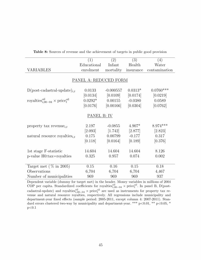
Table 8: Sources of revenue and the achievement of targets in public good provision

(1) (2) (3) (4)Educational Infant Health Water

VARIABLES enrolment mortality insurance contamination

PANEL A: REDUCED FORM

D(post-cadastral-update)i,t 0.0133 -0.000557 0.0313* 0.0760***[0.0134] [0.0109] [0.0174] [0.0219]

royaltiesoili,00−04 × priceoil

t 0.0292* 0.00155 -0.0380 0.0589[0.0176] [0.00166] [0.0304] [0.0762]

PANEL B: IV

property tax revenuei,t 2.197 -0.0855 4.907* 8.974***[2.093] [1.742] [2.877] [2.823]

natural resource royaltiesi,t 0.175 0.00799 -0.177 0.317[0.118] [0.0164] [0.189] [0.376]

1st stage F-statistic 14.604 14.604 14.604 8.126p-value H0:tax=royalties 0.325 0.957 0.074 0.002

Target met ( % in 2005) 0.15 0.16 0.15 0.18Observations 6,704 6,704 6,704 4,467Number of municipalities 969 969 969 937Dependent variable (dummy for target met) in the header. Money variables in millions of 2004COP per capita. Standardized coefficients for royaltiesoili,00−04 × priceoilt . In panel B, D(post-

cadastral-update) and royaltiesoili,00−04 × priceoilt are used as instruments for property tax re-venue and natural resource royalties, respectively. All regressions include municipality anddepartment-year fixed effects (sample period: 2005-2011, except column 4: 2007-2011). Stan-dard errors clustered two-way by municipality and department-year. *** p<0.01, ** p<0.05, *p<0.1

45

Table 9: Sources of revenue and the achievement of targets in public good provision (cu-mulative royalties)

(1) (2) (3) (4)Educational Infant Health Water

VARIABLES enrolment mortality insurance contamination

PANEL A: REDUCED FORM

D(post-cadastral-update)i,t 0.0133 -0.000528 0.0318* 0.0769***[0.0133] [0.0109] [0.0174] [0.0219]∑t

k=2006 royaltiesoili,00−04 × priceoil

k -0.00966 -0.00132 -0.00219 -0.0735[0.0284] [0.00404] [0.0288] [0.0481]

PANEL B: IV

property tax revenuei,t 2.130 -0.0851 5.085* 9.184***[2.090] [1.743] [2.876] [2.827]

natural resource royalties (cum.)i,t -0.00972 -0.000957 -0.00677 -0.0751**[0.0224] [0.00365] [0.0226] [0.0310]

1st stage F-statistic 11.807 11.807 11.807 7.381p-value H0:tax=royalties 0.306 0.962 0.077 0.001

Target met ( % in 2005) 0.15 0.16 0.15 0.18Observations 6,704 6,704 6,704 4,467Number of municipalities 969 969 969 937Dependent variable (dummy for target met) in the header. Money variables in millions of 2004COP per capita. Standardized coefficients for

∑royaltiesoili,00−04 × priceoilt . In panel B, D(post-

cadastral-update) and∑

royaltiesoili,00−04×priceoilt are used as instruments for property tax revenueand cumulative natural resource royalties, respectively. All regressions include municipality anddepartment-year fixed effects (sample period: 2005-2011, except column 4: 2007-2011). Standarderrors clustered two-way by municipality and department-year. *** p<0.01, ** p<0.05, * p<0.1

46

Table 10: Heterogeneous effect of cadastral updates for oil-royalty recipients

(1) (2) (3) (4)Educational Infant Health Water

VARIABLES enrolment mortality insurance quality

PANEL A: natural log of dependent variable

D(post-cadastral-update)i,t 0.00887*** 0.00301 0.0123 -0.119**[0.00334] [0.00210] [0.00855] [0.0559]

D(post-cadastral-update)i,t × royaltiesoili,00−04 -0.000692 -0.00117 -0.00285 0.0216

[0.00109] [0.000873] [0.00284] [0.0312]

p-value H0: effect for median oil royalties=0 0.009 0.174 0.163 0.040p-value H0: effect for average oil royalties=0 0.021 0.375 0.259 0.126

PANEL B: dummy for target met

D(post-cadastral-update)i,t 0.0136 -0.000637 0.0314* 0.0748***[0.0132] [0.0109] [0.0173] [0.0220]

D(post-cadastral-update)i,t × royaltiesoili,00−04 -0.00943 0.00101 0.00397 -0.00224

[0.0129] [0.00171] [0.00795] [0.0174]

p-value H0: effect for median oil royalties=0 0.365 0.964 0.064 0.001p-value H0: effect for average oil royalties=0 0.792 0.978 0.057 0.008

Observations 6,704 6,704 6,704 4,467Number of municipalities 969 969 969 937

Notes: Dependent variable in the header. royaltiesoili,00−04 is standardized: among oil-royalty

recipients (00-04) the mean is 0.93, median is 0.15. All regressions include municipality anddepartment-year fixed effects (sample period: 2005-2011 except column 4: 2007-2011). Standarderrors clustered two-way by municipality and department-year. *** p<0.01, ** p<0.05, * p<0.1

47

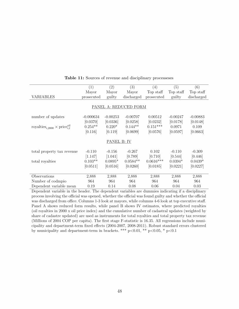
Table 11: Sources of revenue and disciplinary processeses

(1) (2) (3) (4) (5) (6)Mayor Mayor Mayor Top staff Top staff Top staff

VARIABLES prosecuted guilty discharged prosecuted guilty discharged

PANEL A: REDUCED FORM

number of updates -0.000634 -0.00253 -0.00707 0.00512 -0.00247 -0.00883[0.0370] [0.0336] [0.0258] [0.0232] [0.0178] [0.0148]

royaltiesi,2000 × priceoili,t 0.254** 0.220* 0.144** 0.151*** 0.0971 0.109

[0.116] [0.119] [0.0699] [0.0576] [0.0597] [0.0663]

PANEL B: IV

total property tax revenue -0.110 -0.156 -0.267 0.102 -0.110 -0.309[1.147] [1.041] [0.789] [0.710] [0.544] [0.446]

total royalties 0.103** 0.0895* 0.0584** 0.0616*** 0.0394* 0.0439*[0.0511] [0.0516] [0.0260] [0.0185] [0.0221] [0.0227]

Observations 2,888 2,888 2,888 2,888 2,888 2,888Number of codmpio 964 964 964 964 964 964Dependent variable mean 0.19 0.14 0.08 0.06 0.04 0.03Dependent variable in the header. The dependent variables are dummies indicating if a disciplinaryprocess involving the official was opened, whether the official was found guilty and whether the officialwas discharged from office. Columns 1-3 look at mayors, while columns 4-6 look at top executive staff.Panel A shows reduced form results, while panel B shows IV estimates, where predicted royalties(oil royalties in 2000 x oil price index) and the cumulative number of cadastral updates (weighted byshare of cadastre updated) are used as instruments for total royalties and total property tax revenue(Millions of 2004 COP per capita). The first stage F-statistic is 16.35. All regressions include muni-cipality and department-term fixed effects (2004-2007, 2008-2011). Robust standard errors clusteredby municipality and department-term in brackets. *** p<0.01, ** p<0.05, * p<0.1

48

Table 12: Additional effects of oil price shocks

(1) (2) (3) (4)ln Business Murder FARC

VARIABLES population tax rate events

PANEL A: Contemporary shocks

royaltiesoili,00−04 × priceoil

t -0.000188 0.00573 -3.131** 0.594***[0.00191] [0.00485] [1.423] [0.143]

PANEL B: Cumulative shocks∑tk=2006 royaltiesoil

i,00−04 × priceoilk 0.0101*** 0.0149*** -0.558 0.226

[0.00242] [0.00411] [1.929] [0.211]

Observations 6,704 6,704 6,704 5,743Number of municipalities 969 969 969 966Dependent var. mean 30026.40 0.02 33.87 1.37Dependent variable in the header. Money variables in millions of 2004 COP per capita. Allcoefficients are standardized. All regressions include municipality and department-year fixedeffects (sample period: 2005-2011, except column 4: 2005-2010). Standard errors clusteredtwo-way by municipality and department-year. *** p<0.01, ** p<0.05, * p<0.1

49

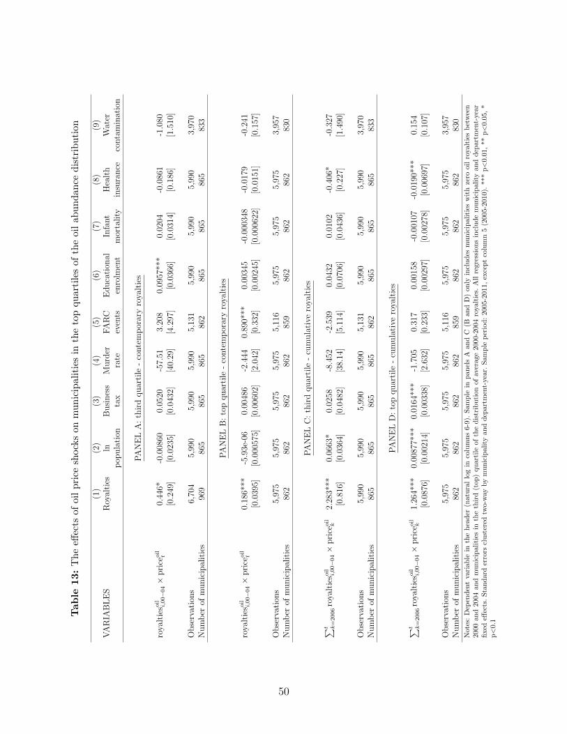
Table

13:

Th

eeff

ects

ofoi

lpri

cesh

ock

son

mu

nic

ipal

itie

sin

the

top

qu

arti

les

ofth

eoi

lab

un

dan

ced

istr

ibu

tion

(1)

(2)

(3)

(4)

(5)

(6)

(7)

(8)

(9)

VA

RIA

BL

ES

Roy

alti

esln

Busi

nes

sM

urd

erFA

RC

Educa

tion

alIn

fant

Hea

lth

Wat

erp

opula

tion

tax

rate

even

tsen

rolm

ent

mor

tality

insu

rance

conta

min

atio

n

PA

NE

LA

:th

ird

quar

tile

-co

nte

mp

orar

yro

yalt

ies

roya

ltie

soili,

00−

04×

pri

ceoilt

0.44

6*-0

.008

600.

0520

-57.

513.

208

0.09

57**

*0.

0204

-0.0

861

-1.0

80[0

.249

][0

.023

5][0

.043

2][4

0.29

][4

.297

][0

.036

6][0

.031

4][0

.186

][1

.510

]

Obse

rvat

ions

6,70

45,

990

5,99

05,

990

5,13

15,

990

5,99

05,

990

3,97

0N

um

ber

ofm

unic

ipal

itie

s96

986

586

586

586

286

586

586

583

3

PA

NE

LB

:to

pquar

tile

-co

nte

mp

orar

yro

yalt

ies

roya

ltie

soili,

00−

04×

pri

ceoilt

0.18

6***

-5.9

3e-0

60.

0048

6-2

.444

0.89

0***

0.00

345

-0.0

0034

8-0

.017

9-0

.241

[0.0

395]

[0.0

0057

5][0

.006

02]

[2.0

42]

[0.3

32]

[0.0

0245

][0

.000

622]

[0.0

151]

[0.1

57]

Obse

rvat

ions

5,97

55,

975

5,97

55,

975

5,11

65,

975

5,97

55,

975

3,95

7N

um

ber

ofm

unic

ipal

itie

s86

286

286

286

285

986

286

286

283

0

PA

NE

LC

:th

ird

quar

tile

-cu

mula

tive

roya

ltie

s

∑ t k=

2006

roya

ltie

soili,

00−

04×

pri

ceoilk

2.28

3***

0.06

63*

0.02

58-8

.452

-2.5

390.

0432

0.01

02-0

.406

*-0

.327

[0.8

16]

[0.0

364]

[0.0

482]

[38.

14]

[5.1

14]

[0.0

706]

[0.0

436]

[0.2

27]

[1.4

90]

Obse

rvat

ions

5,99

05,

990

5,99

05,

990

5,13

15,

990

5,99

05,

990

3,97

0N

um

ber

ofm

unic

ipal

itie

s86

586

586

586

586

286

586

586

583

3

PA

NE

LD

:to

pquar

tile

-cu

mula

tive

roya

ltie

s

∑ t k=

2006

roya

ltie

soili,

00−

04×

pri

ceoilk

1.26

4***

0.00

877*

**0.

0164

***

-1.7

050.

317

0.00

158

-0.0

0107

-0.0

190*

**0.

154

[0.0

876]

[0.0

0214

][0

.003

38]

[2.6

32]

[0.2

33]

[0.0

0297

][0

.002

78]

[0.0

0697

][0

.107

]

Obse

rvat

ions

5,97

55,

975

5,97

55,

975

5,11

65,

975

5,97

55,

975

3,95

7N

um

ber

ofm

unic

ipal

itie

s86

286

286

286

285

986

286

286

283

0N

ote

s:D

epen

den

tva

riab

lein

the

hea

der

(nat

ura

llo

gin

colu

mn

s6-9

).S

am

ple

inp

an

els

Aan

dC

(Ban

dD

)on

lyin

clu

des

mu

nic

ipali

ties

wit

hze

rooil

roya

ltie

sb

etw

een

2000

an

d20

04an

dm

un

icip

alit

ies

inth

eth

ird

(top

)qu

art

ile

of

the

dis

trib

uti

on

of

aver

age

2000-2

004

roya

ltie

s.A

llre

gre

ssio

ns

incl

ud

em

un

icip

ali

tyan

dd

epart

men

t-ye

arfi

xed

effec

ts.

Sta

nd

ard

erro

rscl

ust

ered

two-

way

by

mun

icip

ali

tyan

dd

epart

men

t-ye

ar.

Sam

ple

per

iod

:20

05-2

011,

exce

pt

colu

mn

5(2

005-2

010)

.***

p<

0.0

1,

**

p<

0.0

5,

*p<

0.1

50

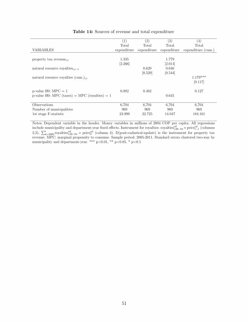
Table 14: Sources of revenue and total expenditure

(1) (2) (3) (4)Total Total Total Total

VARIABLES expenditure expenditure expenditure expenditure (cum.)

property tax revenuei,t 1.335 1.779[2.266] [2.014]

natural resource royaltiesi,t−1 0.629 0.646[0.529] [0.544]

natural resource royalties (cum.)i,t 1.179***[0.117]

p-value H0: MPC = 1 0.882 0.482 0.127p-value H0: MPC (taxes) = MPC (royalties) = 1 0.645

Observations 6,704 6,704 6,704 6,704Number of municipalities 969 969 969 9691st stage F-statistic 23.999 22.725 14.047 184.161

Notes: Dependent variable in the header. Money variables in millions of 2004 COP per capita. All regressionsinclude municipality and department-year fixed effects. Instrument for royalties: royaltiesoil

i,00−04×priceoilt−1 (columns

2,3),∑t

k=2006 royaltiesoili,00−04 × priceoil

k (column 4). D(post-cadastral-update) is the instrument for property taxrevenue. MPC: marginal propensity to consume. Sample period: 2005-2011. Standard errors clustered two-way bymunicipality and department-year. *** p<0.01, ** p<0.05, * p<0.1

51

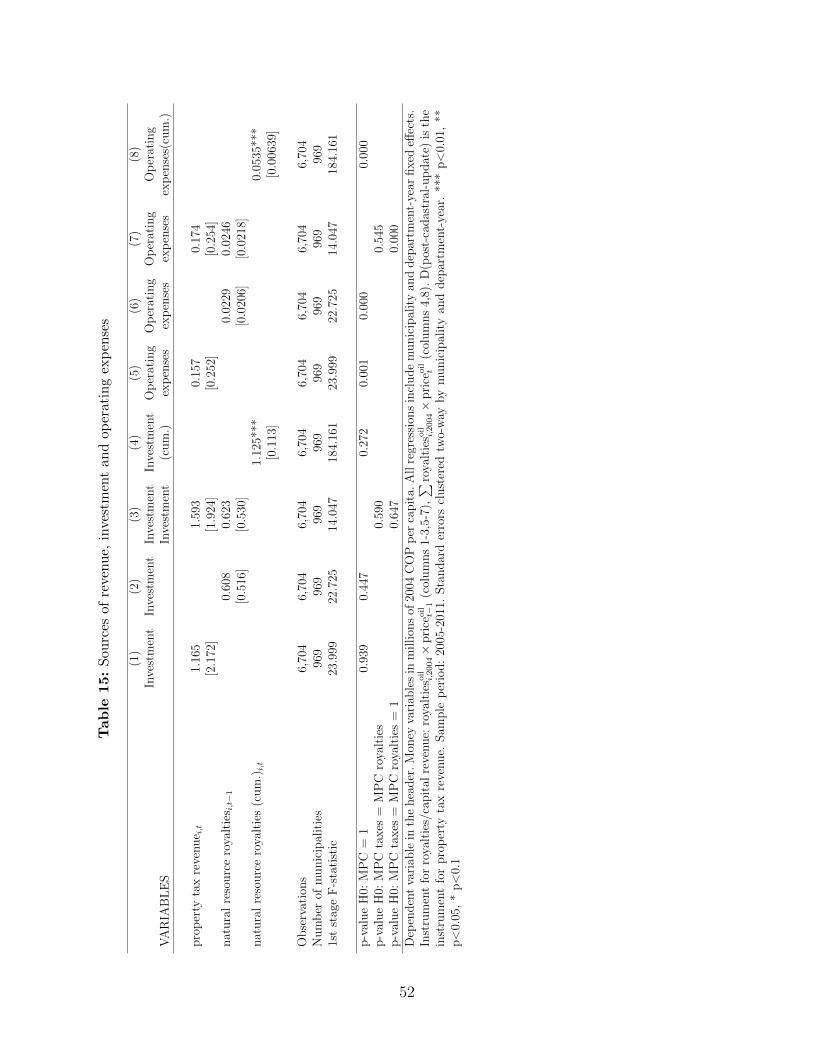
Table

15:

Sou

rces

ofre

venu

e,in

vest

men

tan

dop

erat

ing

exp

ense

s

(1)

(2)

(3)

(4)

(5)

(6)

(7)

(8)

Inve

stm

ent

Inve

stm

ent

Inve

stm

ent

Inve

stm

ent

Op

erat

ing

Op

erat

ing

Op

erat

ing

Op

erat

ing

VA

RIA

BL

ES

Inve

stm

ent

(cu

m.)

exp

ense

sex

pen

ses

exp

ense

sex

pen

ses(

cum

.)

pro

per

tyta

xre

venu

e i,t

1.16

51.

593

0.15

70.

174

[2.1

72]

[1.9

24]

[0.2

52]

[0.2

54]

nat

ura

lre

sou

rce

roya

ltie

s i,t−

10.

608

0.62

30.

0229

0.02

46[0

.516

][0

.530

][0

.020

6][0

.021

8]n

atu

ral

reso

urc

ero

yalt

ies

(cu

m.)i,t

1.12

5***

0.05

35**

*[0

.113

][0

.006

39]

Ob

serv

atio

ns

6,70

46,

704

6,70

46,

704

6,70

46,

704

6,70

46,

704

Nu

mb

erof

mu

nic

ipal

itie

s96

996

996

996

996

996

996

996

91s

tst

age

F-s

tati

stic

23.9

9922

.725

14.0

4718

4.16

123

.999

22.7

2514

.047

184.

161

p-v

alu

eH

0:M

PC

=1

0.93

90.

447

0.27

20.

001

0.00

00.

000

p-v

alu

eH

0:M

PC

taxes

=M

PC

roya

ltie

s0.

590

0.54

5p

-val

ue

H0:

MP

Cta

xes

=M

PC

roya

ltie

s=

10.

647

0.00

0D

epen

den

tva

riab

lein

the

hea

der

.M

oney

vari

able

sin

mil

lion

sof

2004

CO

Pp

erca

pit

a.A

llre

gres

sion

sin

clu

de

mu

nic

ipal

ity

and

dep

artm

ent-

year

fixed

effec

ts.

Inst

rum

ent

for

roya

ltie

s/ca

pit

alre

venu

e:ro

yalt

ieso

ili,

2004×

pri

ceoilt−

1(c

olu

mn

s1-

3,5-

7),∑ ro

yalt

ieso

ili,

2004×

pri

ceoilt

(col

um

ns

4,8)

.D

(pos

t-ca

das

tral

-up

dat

e)is

the

inst

rum

ent

for

pro

per

tyta

xre

venu

e.S

amp

lep

erio

d:

2005

-201

1.S

tan

dar

der

rors

clu

ster

edtw

o-w

ayby

mu

nic

ipal

ity

and

dep

artm

ent-

year

.**

*p<

0.01

,**

p<

0.05

,*

p<

0.1

52

Table 16: Sources of revenue and educational infrastructure

(1) (2) (3) (4)Schools Schools Teaching area Teaching area

VARIABLES per 10,000 inh. per 10,000 inh.

PANEL A: REDUCED FORM

D(post-cadastral-update)i,t 0.897** 0.196 978.2 56.04[0.440] [0.146] [1,134] [236.1]∑t

k=2006 royaltiesoili,00−04 × priceoil

k 0.206 0.0479 637.9 657.1[0.164] [0.142] [1,008] [731.3]

PANEL B: IV

property tax revenuei,t 143.7* 31.38 112,653 7,231[74.43] [25.18] [132,842] [26,888]

natural resource royalties (cum.)i,t 0.0195 0.00653 374.7 548.1[0.149] [0.116] [815.9] [575.3]

1st stage F-statistic 11.807 11.807 5.503 5.503p-value H0:tax=royalties 0.054 0.213 0.399 0.804

Observations 6,704 6,704 3,882 3,882Number of municipalities 969 969 871 871Dependent variable mean 47.69 27.93 10,010.2 4,852.09Dependent variable in the header. Money variables in millions of 2004 COP per capita. Standardized coefficientsfor

∑royaltiesoili,2004 × priceoilt . In panel B, D(post-cadastral-update) and

∑royaltiesoili,2004 × priceoilt are used as

instruments for property tax revenue and cumulative natural resource royalties, respectively. All regressions includemunicipality and department-year fixed effects. Sample period: 2005-2011 (columns 1 and 2), 2006-2011 (columns3 and 4). Standard errors clustered two-way by municipality and department-year. *** p<0.01, ** p<0.05, * p<0.1

53

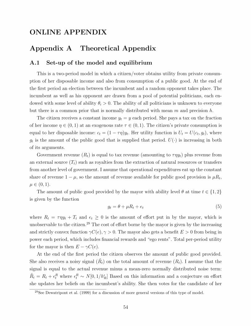
ONLINE APPENDIX

Appendix A Theoretical Appendix

A.1 Set-up of the model and equilibrium

This is a two-period model in which a citizen/voter obtains utility from private consum-

ption of her disposable income and also from consumption of a public good. At the end of

the first period an election between the incumbent and a random opponent takes place. The

incumbent as well as his opponent are drawn from a pool of potential politicians, each en-

dowed with some level of ability θi > 0. The ability of all politicians is unknown to everyone

but there is a common prior that is normally distributed with mean m and precision h.

The citizen receives a constant income yt = y each period. She pays a tax on the fraction

of her income η ∈ (0, 1) at an exogenous rate τ ∈ (0, 1). The citizen’s private consumption is

equal to her disposable income: ct = (1− τη)yt. Her utility function is Ut = U(ct, gt), where

gt is the amount of the public good that is supplied that period. U(·) is increasing in both

of its arguments.

Government revenue (Rt) is equal to tax revenue (amounting to τηyt) plus revenue from

an external source (Tt) such as royalties from the extraction of natural resources or transfers

from another level of government. I assume that operational expenditures eat up the constant

share of revenue 1− µ, so the amount of revenue available for public good provision is µRt,

µ ∈ (0, 1).

The amount of public good provided by the mayor with ability level θ at time t ∈ {1, 2}is given by the function

gt = θ + µRt + et (5)

where Rt = τηyt + Tt and et ≥ 0 is the amount of effort put in by the mayor, which is

unobservable to the citizen.29 The cost of effort borne by the mayor is given by the increasing

and strictly convex function γC(e), γ > 0. The mayor also gets a benefit E > 0 from being in

power each period, which includes financial rewards and “ego rents”. Total per-period utility

for the mayor is then E − γC(e).

At the end of the first period the citizen observes the amount of public good provided.

She also receives a noisy signal (Rt) on the total amount of revenue (Rt). I assume that the

signal is equal to the actual revenue minus a mean-zero normally distributed noise term:

Rt = Rt + εRt where εRt ∼ N [0, 1/hεR] Based on this information and a conjecture on effort

she updates her beliefs on the incumbent’s ability. She then votes for the candidate of her

29See Dewatripont et al. (1999) for a discussion of more general versions of this type of model.

54

liking.

Before making additional assumptions about the link between the sources of revenue and

the noisy signal that the citizen receives, I summarize the timing of the game (I will drop

the time subscripts for everything that is not changing over time):

1. The incumbent (with ability θI unknown to all) receives revenue R = T + τηy and

chooses the amount of effort e1.

2. A quantity of public goods g1 is provided according to equation 5.

3. The citizen observes g1 and receives the noisy signal R. She uses this information to

update her beliefs on the incumbent’s ability: θI .

4. The citizen votes either for the incumbent or for a random opponent with the same

prior ability (m).

5. The winner of the election chooses e2 and this determines g2.

We can find the PBE in pure strategies using backwards induction. The winning candidate

(with ability θ2) solves the following problem in the second period:

maxe2≥0

E − γC(e2)

Since γC(·) is an increasing function, the second-period mayor will set e?2 = 0 and will get

utility E that period. Therefore, the amount of public good provided will be g?2(θ2) = θ2+µR,

which is an increasing function of the ability of the second-period mayor. If the voter chooses

a candidate with believed ability θ, her second period utility is U(c2, g?2(θ)) = U(1− τηy, θ+

µR). Since U(·) is increasing in g2, the incumbent will be re-elected only if the voter believes

him to have higher ability than the opponent. That is, if θI ≥ m.

The citizen updates her beliefs on the incumbent’s ability based on the amount of first-

period public goods (g1), her conjecture on the level of effort put in by the incumbent

(e1), and the noisy signal on revenue (R). The problem that the citizen faces is that the

discrepancy between the observed amount of public goods and the amount she expected,

which I will label Z1 ≡ g1−µR− e1, is equal to the incumbent’s ability (θI) minus the noise

term’s impact on expected public goods (µεRt ). Given that θI and µεRt are two independent

normally distributed random variables, the solution to the signal extraction problem is:

θI = E[θI |Z1] =mh+ Z1hRh+ hR

(6)

55

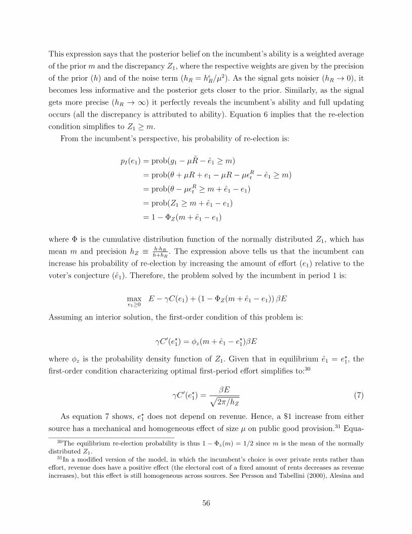
This expression says that the posterior belief on the incumbent’s ability is a weighted average

of the prior m and the discrepancy Z1, where the respective weights are given by the precision

of the prior (h) and of the noise term (hR = hεR/µ2). As the signal gets noisier (hR → 0), it

becomes less informative and the posterior gets closer to the prior. Similarly, as the signal

gets more precise (hR → ∞) it perfectly reveals the incumbent’s ability and full updating

occurs (all the discrepancy is attributed to ability). Equation 6 implies that the re-election

condition simplifies to Z1 ≥ m.

From the incumbent’s perspective, his probability of re-election is:

pI(e1) = prob(g1 − µR− e1 ≥ m)

= prob(θ + µR + e1 − µR− µεRt − e1 ≥ m)

= prob(θ − µεRt ≥ m+ e1 − e1)

= prob(Z1 ≥ m+ e1 − e1)

= 1− ΦZ(m+ e1 − e1)

where Φ is the cumulative distribution function of the normally distributed Z1, which has

mean m and precision hZ ≡ h·hRh+hR

. The expression above tells us that the incumbent can

increase his probability of re-election by increasing the amount of effort (e1) relative to the

voter’s conjecture (e1). Therefore, the problem solved by the incumbent in period 1 is:

maxe1≥0

E − γC(e1) + (1− ΦZ(m+ e1 − e1)) βE

Assuming an interior solution, the first-order condition of this problem is:

γC ′(e?1) = φz(m+ e1 − e?1)βE

where φz is the probability density function of Z1. Given that in equilibrium e1 = e?1, the

first-order condition characterizing optimal first-period effort simplifies to:30

γC ′(e?1) =βE√2π/hZ

(7)

As equation 7 shows, e?1 does not depend on revenue. Hence, a $1 increase from either

source has a mechanical and homogeneous effect of size µ on public good provision.31 Equa-

30The equilibrium re-election probability is thus 1 − Φz(m) = 1/2 since m is the mean of the normallydistributed Z1.

31In a modified version of the model, in which the incumbent’s choice is over private rents rather thaneffort, revenue does have a positive effect (the electoral cost of a fixed amount of rents decreases as revenueincreases), but this effect is still homogeneous across sources. See Persson and Tabellini (2000), Alesina and

56

tion 7 also shows that e?1 is an increasing function of hZ (since C(e) is strictly convex), which

is itself an increasing function of the precision of the revenue signal hR. Hence, as the signal

becomes more precise, the voter becomes more attentive to public good provision and the

incumbent provides more effort in equilibrium.

A.2 Taxes as a source of information on public revenue

Having solved the model, I now examine two extensions that link the source of revenue to

the precision of the revenue signal and yield predictions of a heterogeneous effect of revenue

from different sources on incumbent effort and public good provision. I start by assuming

that the share of exogenous revenue amplifies the noise in the voter’s signal:

Assumption 1. Rt = Rt − εRt where εRt = εt ×(

TT+τηy

) 12

and εt ∼ N [0, 1/hε]

Hence, the precision of the revenue signal is hR =(T+τηyT

)hεµ2

. This assumption captures

the idea that citizens are better informed about changes in tax revenue than about changes

in external revenue. Now, as tax revenue increases, the signal becomes more precise and the

citizen becomes more attentive to the amount of public goods provided in her assessment of

the incumbent’s quality. This in turn makes it optimal for the incumbent to increase effort

in order to influence the election in his favour. By the same logic, an increase in exogenous

revenue makes the revenue signal noisier and the citizen less responsive, so the incumbent

reduces effort.

As before, the functional form of the production function for public goods implies that

revenue from any source has a mechanical effect on public good provision. However, the total

or net effect of a revenue increase depends also on the indirect effect through incumbent effort.

Under assumption 1, an increase in tax revenue has a larger effect on public good provision

than an equivalent increase in external revenue due to the opposite indirect effect through

incumbent effort. The following proposition formalizes this result.

Proposition 1. Under assumption 1, the equilibrium first-period effort of the incumbent is

increasing in tax revenue and decreasing in external revenue. Hence, public good provision in

the first period increases by more than the mechanical revenue effect when there is an increase

in tax revenue and by less than the mechanical revenue effect when there is an increase in

external revenue.

Tabellini (2007), Brollo et al. (2013) or Matsen et al. (2015) for examples. If the incumbent is unconstrainedon the amount he can appropriate, extra revenue has the additional effect of increasing the value of stayingin power. This mechanism is at play in the model of the resource curse in Robinson et al. (2006). Still, thisdoes not give rise to any heterogeneity across sources.

57

Proof. Using the implicit function theorem and noting that C(·) is a strictly convex function,

when we differentiate (7) with respect to τηy we obtain:

γ∂2C

∂e?12

∂e?1∂τηy

=∂φZ∂hZ

∂hZ∂τηy

βE (8)

From φZ =√hZ/2π we can see that ∂φZ/∂hZ > 0. Using the definitions of hZ and hR

we find that∂hZ∂τηy

=(µh)2hεT

(hε(T + τηy) + µ2hT )2 > 0

Since all other terms on both sides of equation 8 are positive,∂e?1∂τηy

> 0. Hence, the overall

effect of a tax revenue increase on first-period public good provision, based on equation 1, is

given by∂g?1∂τηy

= µ+∂e?1∂τηy

> µ

where µ is the mechanical revenue effect.

Using again implicit differentiation on equation (7) but with respect to T we get

γ∂2C

∂e?12

∂e?1∂T

=∂φZ∂hZ

∂hZ∂T

βE (9)

The argument works the same as in the case of taxes, except that now

∂hZ∂T

=−(µh)2hετηy

(hε(T + τηy) + µ2hT )2 < 0

Since all the other terms on both sides of equation 9 are positive,∂e?1∂T

< 0. Therefore,

the overall effect of an increase in exogenous revenue on first-period public good provision is

given by∂g?1∂T

= µ+∂e?1∂T

< µ <∂g?1∂τηy

where again µ is the mechanical revenue effect.

A.3 Taxes as an incentive for information acquisition on public

revenue

I now substitute Assumption 1 with the following three assumptions:

Assumption 2. Rt = Rt + εRt , where εRt ∼ N [0, 1/hεR]

58

Assumption 3. Ut = U(ct +αgt) where U(·) is a strictly concave function and α ∈ (0, 1/µ)

Assumption 4. At the start of the game, the voter can choose how much effort (f1 ≥ 0) to

spend on the improvement of the revenue signal. Effort increases the precision of the revenue

signal according to the linear function hεR = λf1, λ > 0, but has a cost given by the strictly

convex function K(f1)

Under assumptions 2-4 the model is essentially unchanged: the incumbent’s first-period

effort is still determined by (7) and is increasing on the precision of the revenue signal.

If we substitute the public good production function and the voter’s budget constraint

into her first-period utility function we can see that the problem the voter solves is

maxf1≥0

U1 = U(c1 + αg1)−K(f1)

= U [(1− τη)y + α (θI + µ(τηy + T ) + e?1(hZ))]−K(f1)

= U [y + (αµ− 1)τηy + αµT + αθI + αe?1(hZ)]−K(f1)

Assuming an interior solution, the optimal amount of voter effort is implicitly defined by

the following first-order condition:

U ′[y + (αµ− 1)τηy + αµT + αθI + αe?1(hZ)]α∂e?1∂hZ

∂hZ∂hεR

λ = K ′(f ?1 ) (10)

Just like before, the voter is more responsive to public good provision in her assessment

of the incumbent’s quality the better she is informed about revenue. In turn, the incumbent

puts in more effort as the voter becomes more responsive. Under the new assumptions, what

sets this mechanism in motion is information acquisition by the voter, which depends on the

marginal utility of public goods. When tax revenue increases, private consumption mechani-

cally decreases. Although public good provision also increases due to the mechanical revenue

effect, assumption 3 ensures that the marginal utility of the public good increases as well,

which raises the benefit the voter gets from additional incumbent effort.32 External revenue,

on the other hand, has a negative effect on the marginal utility of the public good due to the

positive mechanical revenue effect and the fact that it does not affect the voter’s disposable

income. Hence, extra taxation provides an incentive for more information acquisition while

the opposite holds true for external revenue. The following proposition formalizes this result:

32Assumption 3 implies that taxation for the purpose of public good provision is inefficient in a settingwhere overhead costs are relatively large. This is consistent with the findings of Pritchett and Aiyar (2014),who report that the median cost of one pupil in public elementary school in India is twice as high as in aprivate school, but educational achievement is much lower.

59

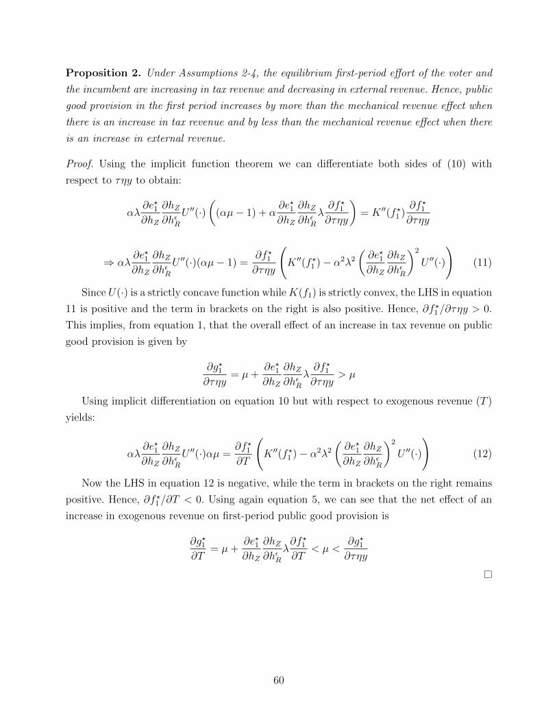
Proposition 2. Under Assumptions 2-4, the equilibrium first-period effort of the voter and

the incumbent are increasing in tax revenue and decreasing in external revenue. Hence, public

good provision in the first period increases by more than the mechanical revenue effect when

there is an increase in tax revenue and by less than the mechanical revenue effect when there

is an increase in external revenue.

Proof. Using the implicit function theorem we can differentiate both sides of (10) with

respect to τηy to obtain:

αλ∂e?1∂hZ

∂hZ∂hεR

U ′′(·)(

(αµ− 1) + α∂e?1∂hZ

∂hZ∂hεR

λ∂f ?1∂τηy

)= K ′′(f ?1 )

∂f ?1∂τηy

⇒ αλ∂e?1∂hZ

∂hZ∂hεR

U ′′(·)(αµ− 1) =∂f ?1∂τηy

(K ′′(f ?1 )− α2λ2

(∂e?1∂hZ

∂hZ∂hεR

)2

U ′′(·)

)(11)

Since U(·) is a strictly concave function whileK(f1) is strictly convex, the LHS in equation

11 is positive and the term in brackets on the right is also positive. Hence, ∂f ?1 /∂τηy > 0.

This implies, from equation 1, that the overall effect of an increase in tax revenue on public

good provision is given by

∂g?1∂τηy

= µ+∂e?1∂hZ

∂hZ∂hεR

λ∂f ?1∂τηy

> µ

Using implicit differentiation on equation 10 but with respect to exogenous revenue (T )

yields:

αλ∂e?1∂hZ

∂hZ∂hεR

U ′′(·)αµ =∂f ?1∂T

(K ′′(f ?1 )− α2λ2

(∂e?1∂hZ

∂hZ∂hεR

)2

U ′′(·)

)(12)

Now the LHS in equation 12 is negative, while the term in brackets on the right remains

positive. Hence, ∂f ?1 /∂T < 0. Using again equation 5, we can see that the net effect of an

increase in exogenous revenue on first-period public good provision is

∂g?1∂T

= µ+∂e?1∂hZ

∂hZ∂hεR

λ∂f ?1∂T

< µ <∂g?1∂τηy

60