WP/09/46

Sovereign Default, Private Sector Creditors and the IFIs

Emine Boz

© 2009 International Monetary Fund WP 09/46 IMF Working Paper IMF Institute Sovereign Default, Private Sector Creditors and the IFIs

Prepared by Emine Boz1

Authorized for distribution by Alexandros Mourmouras

March 2009

Abstract

This Working Paper should not be reported as representing the views of the IMF. The views expressed in this Working Paper are those of the author(s) and do not necessarily represent those of the IMF or IMF policy. Working Papers describe research in progress by the author(s) and are published to elicit comments and to further debate.

This paper builds a model of a sovereign borrower that has access to credit from private sector creditors and an IFI. Private sector creditors and the IFI offer different debt contracts that are modelled based on the institutional frameworks of these two types of debt. We analyze the decisions of a sovereign on how to allocate its borrowing needs between these two types of creditors, and when to default on its debt to the private sector creditor. The numerical analysis shows that, consistent with the data; the model predicts countercyclical IFI debt along with procyclical commercial debt flows, also matching other features of the data such as frequency of IFI borrowing and mean IFI debt stock. JEL Classification Numbers: F33, F34, G15 Keywords: emerging markets, sovereign debt and default, IFIs Author’s E-Mail Address: EBoz@imf.org

1 I am grateful to Sheila Bassett, Pelin Berkmen, Enrica Detragiache, Ceyhun Bora Durdu, Chris Jarvis, Anton Korinek, Leslie Lipschitz, Enrique Mendoza, Ydahlia Metzgen, Alex Mourmouras, Marco Rossi as well as the participants of the World Congress of the International Economic Association in Istanbul, European Meetings of the Econometric Society in Milan, and IMF Institute Lunch Seminar for helpful comments and suggestions.

- 2 -

Contents

I. Introduction . . . . . . . . . . . . . . . . . . . . . . . . . . . . . . . . . . . . . 3

II. IMF Lending . . . . . . . . . . . . . . . . . . . . . . . . . . . . . . . . . . . . . 6A. Institutional Framework . . . . . . . . . . . . . . . . . . . . . . . . . . . 6B. Cyclical Properties . . . . . . . . . . . . . . . . . . . . . . . . . . . . . . 7

III. Model . . . . . . . . . . . . . . . . . . . . . . . . . . . . . . . . . . . . . . . . . 10

IV. Quantitative Analysis . . . . . . . . . . . . . . . . . . . . . . . . . . . . . . . . 13A. Solution . . . . . . . . . . . . . . . . . . . . . . . . . . . . . . . . . . . . 13B. Calibration and Data . . . . . . . . . . . . . . . . . . . . . . . . . . . . . 14C. Findings . . . . . . . . . . . . . . . . . . . . . . . . . . . . . . . . . . . . 15D. Sensitivity Analysis . . . . . . . . . . . . . . . . . . . . . . . . . . . . . . 17

V. Conclusion . . . . . . . . . . . . . . . . . . . . . . . . . . . . . . . . . . . . . . 18

Appendices . . . . . . . . . . . . . . . . . . . . . . . . . . . . . . . . . . . . . . . . . 19

References . . . . . . . . . . . . . . . . . . . . . . . . . . . . . . . . . . . . . . . . . . 20

Tables

1. Average interest rates . . . . . . . . . . . . . . . . . . . . . . . . . . . . . . . . 222. Data Moments: Private Sector Creditor Lending . . . . . . . . . . . . . . . . . 223. Data Moments: IMF Lending . . . . . . . . . . . . . . . . . . . . . . . . . . . . 234. Spreads and Use of IMF Credit . . . . . . . . . . . . . . . . . . . . . . . . . . . 235. Probability of Use of IMF Credit . . . . . . . . . . . . . . . . . . . . . . . . . . 246. Parameters . . . . . . . . . . . . . . . . . . . . . . . . . . . . . . . . . . . . . . 247. Business Cycle Statistics . . . . . . . . . . . . . . . . . . . . . . . . . . . . . . 258. IFI Debt During High and Low Spreads . . . . . . . . . . . . . . . . . . . . . . 259. IFI Debt During Booms and Busts . . . . . . . . . . . . . . . . . . . . . . . . . 2510. Sensitivity . . . . . . . . . . . . . . . . . . . . . . . . . . . . . . . . . . . . . . 26

Figures

1. IMF Interest Rates vs U.S. Government Bond Yields . . . . . . . . . . . . . . 262. Commercial Debt Price Schedule, q(d′, d∗′, y) . . . . . . . . . . . . . . . . . . . 273. Stationary Bond Distributions for the Simple SOE Model . . . . . . . . . . . . 27

- 3 -

I. Introduction

Sovereign borrower and creditor relationships have long been complicated by sovereigns’incentives to default on their debt.1 This paper contributes to the literature on sovereigndebt and default by documenting the cyclical properties of lending by InternationalFinancial Institutions (IFIs) and introducing an IFI to a model with strategic default oncommercial debt. The goal of the paper is to uncover the sovereign’s allocation of itsfinancing needs between private sector creditors and the IFI, as well as to account for thecyclical properties of IFI lending.2

Taking the International Monetary Fund (IMF) as an example, the data reveal that thecyclical properties of lending by IFIs are in stark contrast with those of private sectorcreditor lending. The average correlation of IMF debt flows with output for a group ofemerging market economies is -0.15, while the same correlation in the case of commercialdebt flows is 0.37.3 In addition, the variability of commercial debt flows is about threetimes as large as that of IMF debt. Finally, countries do not borrow from the IMF at alltimes; we find the unconditional probability of the use of IMF credit to be around 50percent. This is also in contrast with commercial debt, as all countries in our sample wereindebted to private sector creditors at all times.

Motivated by these regularities, we propose an incomplete markets framework thatfeatures a sovereign, private sector creditors, and an IFI. The sovereign cannot commit torepay its debt to private sector creditors and thereby strategically defaults depending onthe level of its commercial debt, official debt, and output. Punishment for default isexclusion from the commercial credit markets and direct output losses. Assumingperfectly competitive, risk-neutral private sector creditors, the interest rate charged byprivate creditors is determined by endogenous default probabilities.

The IFI offers a different contract than the private sector creditors. These differences arebased on the institutional framework of the IMF loans, more specifically Stand-ByArrangements (SBAs). First, the sovereign can commit to repay its debt to the IFI. Inother words, contracts with the IFI are enforceable while those with commercial creditorsare not. This is loosely implied by the IFI having a preferred creditor status and also thefact that the IMF has almost always been repaid particularly by the emerging marketeconomies that we focus on in this paper. Second, the interest rate associated with IFIlending is assumed to be the sum of the risk free rate and a charge that increases with theamount borrowed from the IFI. This specification for the IFI interest rate captures thesurcharges that may apply in the case of SBAs depending on the amount borrowed.4 Notethat this is significantly different from commercial interest rates, as those depend on theendogenous default probability determined by the “riskiness” of the sovereign. Finally,conditionality associated with IFI debt is accounted for by a higher discount factor inperiods when the sovereign is indebted to the IFI. In this setting, the higher discountfactor tilts the consumption profile by shifting consumption from the present to the

1Reinhart, Rogoff and Savastano (2003) document that sovereigns borrowed and defaulted since the 19thcentury with the maximum number of defaults incurred by Venezuela (9) and Mexico (8).

2Throughout the paper, we use the term “commercial debt” to refer to debt to the private sector creditorand “official debt” to refer to debt to the IFI.

3See Section 2 for more details on the data and calculations.4See Section 2 for details of the institutional framework of SBAs.

- 4 -

future, thereby lowering debt levels and default probabilities. This can be interpreted assimilar to implementing tighter fiscal policies that have traditionally been part of IMFconditionality.5

The model featuring the aforementioned types of creditors, when calibrated to Argentina,a representative emerging market economy, performs well in matching several features ofthe data. First, it generates procyclical commercial debt as well as countercyclical IFIdebt. In good times, the sovereign finds it optimal to borrow more commercially atrelatively lower rates, with lower default probability and without incurring the costsassociated with borrowing from the IFI. However, in bad times, in order to avoid the highrisk premia charged by private sector creditors, the sovereign reallocates its portfolio bygiving more weight to borrowing from the IFI.

The sovereign’s default probability increases with the level of official debt as it does withcommercial debt. The relationship between the default probability and commercial debthas already been established in the literature. With regards to official debt, there are twoeffects working in opposite directions. Ceteris paribus, higher IFI debt in the currentperiod implies higher total debt service in the following period. With high debt service inthe following period, the sovereign is more likely to default on commercial debt to avoidlow levels of consumption. This channel suggests that the higher the IFI debt, the higherthe default probability on commercial debt. Second, positive IFI debt forces the sovereignto discount the future less and act more prudently lowering default probabilities. In thissetting, we find that the first effect is quantitatively larger generating higher countryspreads when the sovereign is indebted to the IFI as opposed to when it is not.6

The elasticity of interest rates to official debt is lower than commercial debt. Highercommercial debt increases default probability significantly, as the benefit of default is thecommercial debt that is forgiven. In the case of official debt, as mentioned above, higherofficial debt the current period increases total debt service in the following period, makingthe sovereign more likely to default to avoid low consumption levels. This channel is lessdirect. The sovereign internalizes the effect of its borrowing on interest rates andacknowledges these different elasticities, therefore, reallocates its portfolio in response tooutput shocks.

Our paper is closely related to the literature on sovereign debt, particularly emergingmarket debt that builds on the seminal work of Eaton and Gersovitz (1981). Recently,Arellano (2008) studied the quantitative implications of Eaton and Gersovitz’s setup afterintroducing stochastic output and exclusion from capital markets for a period withstochastic length and direct output losses as punishment for default. This framework hasalso been extended to include trend shocks to output and debt renegotiation by Aguiarand Gopinath (2006) and Yue (2005), respectively. However, this literature overlooks theexistence of IFIs in credit markets and the role they might play in the sovereign’s debt

5In good times, countries may not have access to borrowing from an IFI. The IMF, for example, agrees toan SBA only when a country has balance of payments difficulties. To account for this, one can assume thatIFI lending is available only when output falls below a certain level and the interest rates charged by theprivate sector creditors exceed a threshold. However, in equilibrium, these constraints would not be bindingbecause the sovereign never chooses to borrow from the IFI if these conditions are not met.

6Note that we only establish correlation but not causality between spreads on commercial debt and IFIlending. In our setting, higher commercial spreads coupled with higher IFI lending are generated by negativeendowment shocks which are the only underlying “cause” of fluctuations.

- 5 -

and default decisions. To our knowledge, the only analysis in this area is conducted byAguiar and Gopinath (2006) who analyze the implications of a third party bailout limitedto a ratio of the defaulted debt. In their extension, this third party is not explicitlymodelled and the bailout takes the form of a grant that is never repaid. In contrast, weexplicitly model the third party as an international financial institution that lends withterms similar to SBAs of the IMF.

An incomplete list of other studies in the sovereign debt literature include Bai and Zhang(2005), Guimaraes (2006), Alfaro and Kanczuk (2007), Arellano and Ramanarayanan(2008), and Mendoza and Yue (2008). Alfaro and Kanczuk (2007) introduce internationalreserves into the standard strategic default model and allow the sovereign to smooth itsconsumption during autarky by using these reserves. This extension is similar to ours inthe sense that it also brings in an additional instrument that is available during autarkyperiods. However, reserve holding is different in spirit because it has a lower bound ofzero. With this lower bound, the authors find that it is optimal for the sovereign not tohold any reserves. With the discount rate much higher than the interest rate on reserves(as usually assumed in the sovereign debt literature), they conclude that zero reserveaccumulation is optimal. On the contrary, in our setup, the sovereign is assumed to be anet debtor vis-a-vis the IFI, making it possible to obtain a well-defined stationarydistribution for this type of debt.

Our modelling of different discount factors for the sovereign is reminiscent of the strategiesused by Cole et. al (1995), Alfaro and Kanczuk (2005), Hatchondo, Martinez, Sapriza(2007) and D’Erasmo (2008) to model “patient vs. impatient” or “aligned vs. misaligned”governments using different discount factors. In other words, conditionality implies thatthe sovereign has to act as a patient/aligned type as long as it is indebted to the IFI. Animportant difference between our model and those utilized in the aforementioned studies isthat in those models different types of governments alternate in power stochastically, whilein ours, the sovereign in some sense chooses its type endogenously because we assume thatthe sovereign acknowledges that it has to act as a patient/aligned type as long as it isindebted to the IFI. And being indebted to the IFI is a choice made by the sovereign.

In our study, we abstract from any informational role that an IMF program might playand, as a result, from any catalytic effect that such a program might have. There is anextensive literature on this topic where the debate is centered around whether IMFlending helps countries avoid or mitigate crises by reducing domestic political costs ofadjustment or whether it exacerbates moral hazard. Cottarelli and Giannini (2002) andGhosh et. al. (2002) provide empirical evidence suggesting that IMF assistance leads tolittle increase in private sector flows, suggesting a minor catalytic role, if any. Mody andSaravia (2006) find that whether IMF programs provide a positive signal depends on thelikelihood that these programs lead to policy adjustments. In the theoretical literature,Morris and Shin (2006) and Corsetti, Guimaraes, and Roubini (2006) analyze theconditions under which the catalytic role exists using a global games framework. Finally,Jeanne and Zettelmeyer (2004) study the effects of IMF assistance on debtor moralhazard. In our model, the IFI lends during exclusion from capital markets and serves asan alternative source of funding which the sovereign utilizes to avoid high interest rates inbad times. By modeling the IFI this way, we abstract from any catalytic effect.

Finally, there is a related literature analyzing the impact of IMF programs on countries’

- 6 -

macroeconomic conditions. Eichengreen, Gupta and Mody (2006) provide acomprehensive survey of this literature and investigate potential links between suddenstops (severeness and probability) and IMF programs. The authors find that IMFprograms somewhat reduce the incidence of sudden stops.

For the rest of the paper we take the International Monetary Fund (IMF) as therepresentative IFI and focus on the properties of its lending. The paper is organized asfollows: Section II documents the institutional framework of IMF lending and the cyclicalproperties of IMF and private sector creditor lending for a set of emerging marketeconomies. Section III describes the benchmark two creditor model. Section IV elaboratesthe solution, describes our calibration, reports model statistics comparing them with thedata, and conducts a sensitivity analysis. Section V concludes.

II. IMF Lending

A. Institutional Framework

The IMF lends to member countries with balance of payments difficulties to provide themwith temporary financing.7 Lending of the IMF involves “conditionality,” that is, theborrower needs to follow appropriate policies to resolve the balance of payments problems.Conditionality is aimed at enabling the borrower to repay the IMF on time.

The amount borrowed from the IMF determines the level of conditionality as well as theinterest rate. Borrowing up to 25 percent of quota involves essentially no conditionality.8

Any amount beyond the 25 percent threshold requires the borrower to propose a policyprogram described in a letter of intent, also called an IMF arrangement or program. IMFlending to provide funding in the face of balance of payments difficulties takes place underthe General Resources Account which include the SBAs usually lasting 4-6 quarters withrepayment in 3-5 years.

The interest rate associated with SBAs is the sum of the Special Drawing Rights (SDR)interest rate, margin, burden sharing adjustment, service fee, commitment fee andsurcharges.

• SDR interest rate is a weighted average of the 3-month U.S. T-bill rate, 3-month UKT-bill rate, Japanese Government 13-week financing bills, and 3-month Eurepo rate.

• Margin is intended to cover the intermediation costs of the IMF and help buildreserves against credit risk. It is set at the beginning of every fiscal year by themanagement of the IMF. The average from May 1993-September 2008 is 62 bps andit is currently set at 100 bps.9

7There is also lending to low-income countries for poverty reduction. In this paper, we focus on emergingmarkets that borrow for balance of payments reasons and the types of loans that are available to them.

8Each member is assigned a quota when it enters the IMF. Quotas are largely based on the size of thecountry determining the voting power of countries and their borrowing limits.

9The margin was negative for 1981-May 1993 since the rate of charge was not based on the SDR rateand the imputed margin for that period is negative.

- 7 -

• A charge for burden sharing is added to cover losses due to over-due obligations tothe IMF. These charges are refunded as overdue obligations are repaid. The averageof the burden sharing adjustment from May 1986-September 2008 is 19 bps and it iscurrently set at 2 bps.

• A service fee of 50 bps apply to cover part of the intermediation costs and this fee ispaid at the time the loan is disbursed.

• A commitment fee is collected but refunded as the loans are withdrawn.10 This fee is25 bps for loans up to the country’s quota, and 10 bps for those in excess of thequota.

• In the case of SBAs, a surcharge of 100 bps apply to the portion of those loans thatare greater than 200 percent of the country’s quota, and 200 bps for the portiongreater than 300 percent.

The sum of the SDR interest rate, margin, and burden sharing adjustment is called theadjusted rate of charge plotted in Figure 1 with historical averages reported in Table 1.Both in the table and the figure, the IMF’s adjusted rate of charge is compared againstU.S. government bonds with 2, 3, and 5-year maturities since under SBAs, the loans arerepaid within 3-5 years. The averages for the IMF’s adjusted rate of charge are in linewith the yield on 3-year U.S. government bonds. This result is somewhat expected giventhat the SDR interest rate constitutes a significant portion of the adjusted rate of chargeand the SDR rate itself is a weighted average of developed country T-bill rates withshorter maturities. Similarly, Jeanne and Zettelmeyer (2001) conclude that the IMF’snon-concessional lending rates, which include SBAs, are comparable to the risk free rate.

Note that the adjusted rate of charge and the above mentioned fees do not vary acrosscountries. The only loan or country specific component of interest rates associated withSBAs is surcharges. These are determined by the size of the loan compared to thecountry’s quota but not by the riskiness of a sovereign.

Another important feature of IMF lending is conditionality. IMF program relatedconditions include macroeconomic and structural measures that fall under the core areasof IMF’s expertise. According to IMF (2002a), these areas are “...macroeconomicstabilization, monetary, fiscal and exchange rate policies, including the underlyinginstitutional arrangements and closely related structural measures, and financial systemissues related to the functioning of both domestic and international financial markets.”IMF (2002b) reports that about 34 percent of the structural measures were regarding thefiscal sector from 1994-1999 followed by financial sector and privatization related measuresthat constituted 16 and 14 percent of total measures, respectively.

B. Cyclical Properties

Although cyclical properties of commercial debt flows have been extensively studied in theliterature, those of IMF lending have remained largely unexplored. In this section, we

10Therefore, commitment is with regards to borrowing from the IMF rather than repayment.

- 8 -

examine these properties for a set of emerging market economies and document ourfindings in Tables 3, 4, and 5. We choose the countries in our sample based on quarterlyGDP data availability and on whether the country had an IMF program in the last twodecades. Table 2 reports the main business cycle statistics associated with commercialdebt for comparison with IMF lending.

Table 2 establishes that commercial debt flows are procyclical, highly variable and, onaverage, most sovereigns in our sample appear to be highly indebted to private sectorcreditors. Net debt flows by private sector creditors data reported in Table 2 are annualand are from the World Bank’s Global Development Finance Database (includes bonds,commercial banks, other debt to private creditors). Their standard deviations andcorrelations with the corresponding country’s real GDP are reported in the third andfourth columns of the Table and the fifth column documents the mean commercial debtstock. On average, the correlation of net lending by private sector creditors with realoutput is 0.37. This correlation is positive for all of the countries in the sample, lyingbetween 0.14 (Peru) and 0.62 (Thailand and Turkey). The average standard deviation ofthis type of lending is 3.71 with Thailand being an outlier with a standard deviation of10.10 percent. Finally, commercial debt stock is around 15 percent of annual GDP onaverage.

Contrary to lending by private sector creditors, IMF lending is countercyclical with anaverage correlation of -0.15 with output.11 Using quarterly data on the use of IMF creditfrom International Financial Statistics (IFS), the second column of Table 3 reveals thatcountercyclicality holds for all countries except Thailand (0.18).12 For the case ofThailand, this statistic may be uninformative since Thailand’s average IMF debt to GDPratio was only 0.14 percent in the period for which quarterly GDP data are available(1993-2006).

The standard deviation of IMF debt flows reported in the third column of the same tablesuggest that IMF debt flows are remarkably less variable than commercial debt flows (1.22vs 3.71). Comparing the debt ratios, mean debt to the IMF is lower than that to theprivate sector creditors (16 vs. 6 percent). Also note that IMF debt ratios are calculatedusing quarterly GDP whereas debt to private sector creditors is divided by annual GDPwhich implies that IMF debt comparable with the 16 percent private sector creditor debtwould be around 1.6 percent. Therefore, on average, IMF debt is around one tenth ofprivate sector creditor debt.13

Table 4 reports statistics on the relationship between the use of IMF resources andcountry spreads based on J.P. Morgan’s EMBI Global spread data from Bloomberg. Sincethe first observation of spread data varies across countries, we report in the second columnof the table, the periods considered in the calculations. The following two columnscompare the average EMBI spreads for periods when there was positive use of Fund

11The finding, that in bust periods a country is more likely to have an IMF program, is not to say thatone causes the other. Correlation does not imply causality.

12Real GDP series are also from IFS. They are logged, deseasonalized using Census X12, and HP filteredwith smoothing parameter 1600. Availability of quarterly GDP data differs among countries, therefore wereport in Table 3 the periods considered for each country.

13These results are in line with Ratha (2001) who finds that during 1996-1998, private flows to developingcountries were 10-12 times multilateral flows.

- 9 -

resources with those when the country was not using Fund resources. The number ofobservations are reported in parenthesis.

Note that of the available sample of EMBI data, only Mexico and Thailand had asignificant number of periods with and without use of Fund resources. For both of thesecountries spreads in periods with use of Fund credit are about 3 times the spreads inperiods without Fund credit. All other countries were indebted to the IMF during asignificant portion of the sample period. We find average spreads to be 617 (199) bpswhen Mexico (Thailand) was using Fund resources, while the average spreads were 242(61) bps when it was not. Suspecting that the spread data might have outliers duringcrises, we also calculate median spreads and find these to be 488 (163) bps in periodswhen Mexico (Thailand) was indebted to the IMF versus 214 (58) bps when it was not.Finally, we compute the correlation between spreads and a dummy variable that is setequal to 1 when the country is indebted to the IMF. We find this correlation to bepositive for all countries in our sample except Ecuador with an average of 0.48.14

These results on the relationship between spreads and IMF borrowing appear to be in linewith those of Mody and Saravia (2006). Mody and Saravia (2006) find that spreads onbonds issued during an IMF arrangement are higher. The authors collect data on launchspreads for more than 3,000 emerging market and developing country bonds and separatethem based on whether they were issued during an IMF program or not. Theircalculations reveal that the spreads during IMF programs were 406, while they were 223in the absence of programs.

IMF borrowing displays lumpiness in the sense that it spikes after a country enters anarrangement with the IMF. These periods of high borrowing are nested in periods withoutany borrowing from the IMF. This kind of pattern manifests itself as a higher standarddeviation of net IMF flows relative to another series with a smoother pattern. In additionto the standard deviation already reported in Table 3, we also calculate the probability ofpositive use of IMF resources from its GRA account (Pr[d∗ > 0]) to get a sense of theaverage length of periods with and without IMF borrowing. Table 5 documents that theunconditional probability of having an arrangement with the IMF is 46 percent for1945-2007 and 55 percent for 1970-2007 when we expand our sample to 17 emergingmarket economies. The rationale for expanding our sample for this exercise is to get amore unbiased picture because one of our selection criteria for the initial sample was toinclude countries with significant IMF borrowing in the last several decades. So byconstruction, the probability of the use of IMF credit would be biased upwards. Theadditional countries included in the calculation of the mean reported in the last row ofTable 5 are Chile, Colombia, Egypt, India, Korea, Malaysia, Singapore, and Venezuela.Note that these probabilities are higher for our original sample with 9 countries.15

Essentially, all IMF loans to major emerging market economies have been repaid.14Averages reported in the last row for E[s|d∗ > 0] and E[s|d∗ = 0] are weighted by the number of

observations. The average for ρ(Id∗>0, s) includes only those countries with at least 4 observations withoutuse of Fund credit (Argentina, Brazil, Mexico, and Thailand).

15Barro and Lee (2005) calculate the fraction of time that a country had an IMF loan program (SBA orEEF) to be 0.185 percent using data for 130 countries from 1975-1999. They also calculate the IMF loanapproval frequency to be 0.364. Approval frequency is calculated by assigning ‘1’ if the country had a loanapproved within a 5-year interval. Our numbers differ from theirs mainly because we focus only on largeemerging market economies and also our dummy is based on quarterly data rather than 5-year intervals.

- 10 -

Zettelmeyer (2005) indicates: “In the past, the IMF has virtually always been repaid, butthis leaves the possibility that currently open lending relationships may eventually resultin arrears or debt forgiveness.” Jeanne and Zettelmeyer (2001) find that “most openlending relationships with emerging market countries are statistically similar to pastlending cycles that eventually ended in repayment while the very long open lending cyclesof many poor countries statistically ‘look’ like they might continue forever.” Similarly,Eichengreen (2003) and Saravia (2004) argue that the IMF loans are typically repaid.Only during the debt crises of the 1980s, was there an increase in non-repayment cases.According to Zettelmeyer (2005), there were 13 countries in protracted arrears to theIMF.16 However, most of these countries have repaid and in particular Peru has repaidwhich is the only emerging market among these countries.

To summarize, this section establishes that:

• The IMF lending rate under SBAs can be approximated by the sum of the risk freerate and a charge that increases with the amount borrowed.

• Lending by private sector creditors is procyclical whereas IMF lending iscountercyclical.

• Debt to the private sector creditors is about three times more variable than that tothe IMF.

• The average debt stock to the IMF is about one tenth of the debt to private sectorcreditors.

• Country spreads are higher in periods when countries are indebted to the IMF.

• The unconditional probability of the use of IMF resources is about 50 percent foremerging markets.

• IMF has almost always been repaid particularly by emerging market economies.

III. Model

The model features competitive, risk-neutral private sector creditors, an IFI, and asovereign that maximizes the utility of its households. The model mainly builds on thework of Eaton and Gersovitz (1981) on sovereign debt with potential repudiation. Thedistinguishing and appealing feature of this framework is the lack of commitment of thesovereign to repaying its debt. Due to this commitment problem, the sovereign mayoptimally default on its debt to the private sector creditors. Therefore, this modelanalyzes a “willingness to pay” scenario rather than “ability to pay.”

Every period, the sovereign is in one of two states: default or non-default vis-a-vis theprivate sector creditors, D, N . If it starts in the non-default state, the sovereign hasaccess to borrowing commercially. In these non-default states, it observes its output level,

16Cambodia, Guyana, Haiti, Honduras, Liberia, Panama, Peru, Sierra Leone, Somalia, Sudan, Vietnam,Zaire, and Zambia.

- 11 -

makes a decision on whether to default or not, and also whether to borrow from the IFI. Ifit chooses to default, it does not repay its existing debt, but as a punishment, it losesaccess to commercial borrowing for a period with exogenously and stochasticallydetermined length. If it does not default, however, it repays its debt obligations in full,chooses how much to borrow commercially and from the IFI, and maintains the option todefault in the following period. During exclusion from commercial borrowing, thesovereign only chooses whether to borrow from the IFI based on its output remaining afterincurring losses due to default.

The IFI lends to the sovereign at the risk free rate plus a debt elastic component that isintended to capture the surcharges of the IMF.17 The sovereign does not face acommitment problem in repaying its debt to the IFI because of the preferred creditorstatus of the IMF and also the observation that major emerging market economies havealmost always repaid their debt to the IMF. There is only one IFI with a non-profit role asan international financial institution in this context.

In our setup, the existence of the IFI provides the sovereign with an additional instrumentto smooth consumption that is available even during exclusion from commercial creditmarkets. Borrowing from the IFI is preferable in times when the default probability onprivate sector debt is high (and as a result the interest rate is high) or when the sovereignis in default and does not have access to commercial credit markets at all.

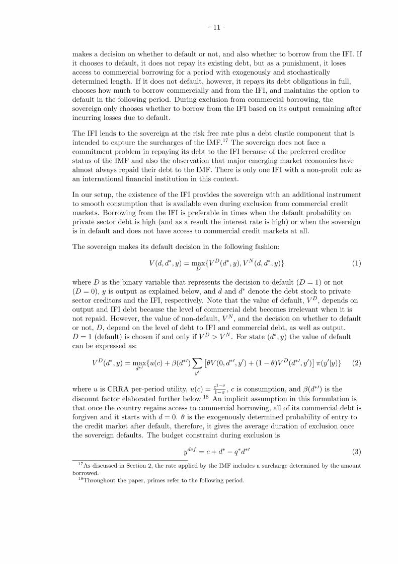
The sovereign makes its default decision in the following fashion:

V (d, d∗, y) = maxD{V D(d∗, y), V N (d, d∗, y)} (1)

where D is the binary variable that represents the decision to default (D = 1) or not(D = 0), y is output as explained below, and d and d∗ denote the debt stock to privatesector creditors and the IFI, respectively. Note that the value of default, V D, depends onoutput and IFI debt because the level of commercial debt becomes irrelevant when it isnot repaid. However, the value of non-default, V N , and the decision on whether to defaultor not, D, depend on the level of debt to IFI and commercial debt, as well as output.D = 1 (default) is chosen if and only if V D > V N . For state (d∗, y) the value of defaultcan be expressed as:

V D(d∗, y) = maxd∗′

{u(c) + β(d∗′)∑

y′

[θV (0, d∗′, y′) + (1− θ)V D(d∗′, y′)

]π(y′|y)} (2)

where u is CRRA per-period utility, u(c) = c1−σ

1−σ , c is consumption, and β(d∗′) is thediscount factor elaborated further below.18 An implicit assumption in this formulation isthat once the country regains access to commercial borrowing, all of its commercial debt isforgiven and it starts with d = 0. θ is the exogenously determined probability of entry tothe credit market after default, therefore, it gives the average duration of exclusion oncethe sovereign defaults. The budget constraint during exclusion is

ydef = c + d∗ − q∗d∗′ (3)17As discussed in Section 2, the rate applied by the IMF includes a surcharge determined by the amount

borrowed.18Throughout the paper, primes refer to the following period.

- 12 -

where q∗ is the price of IFI debt which can be written as:

q∗(d∗′) =1

1 + r + φ(d∗′). (4)

Note that this price depends only on d∗′ and not on d′ or y.

Output is exogenous and is characterized by an AR(1) process:

y = ez (5)

where zt = ρzt−1 + εt and ε ∼ N(0, σ2z). We approximate this Normal process with a

Markov chain with S states and transition probability matrix π. π(yj |yi) denotes theprobability of transiting from state i to j.

The output process is truncated during default as in Arellano (2008) in order to bring thedefault probability implied by the model in line with those in the data. We assume thatthe direct output cost of default increases with output. In other words, if a countrydefaults when its output is high, the output loss due to the default decision would behigher as opposed to a sovereign that defaults when its output is low. Mathematically:

ydef ={

y, if y < yy, if y > y.

In non-default periods, the sovereign decides whether or not to default, and how toallocate its financing needs among the private sector creditors and the IFI. The value ofnon-default in this setup can be written as:

V N (d, d∗, y) = maxd′,d∗′

{u(c) + β(d∗′)∑

y′V (d′, d∗′, y)π(y′|y)} (6)

subject to the budget constraint:

c = y − d + qd′ − d∗ + q∗d∗′. (7)

As mentioned above, the risk neutral and perfectly competitive private sector creditorslend at a rate that is mainly determined by the default probability of the sovereign. Thecommercial bond price schedule is given by:

q(d′, d∗′, y) =1− E[λ(d′, d∗′, y)]

1 + r. (8)

and the spread is defined as s = 1/q − 1− r.

In order to capture the conditionality of IMF loans, and also to account for the regularitythat sovereigns do not borrow from the IMF every period as documented in Table 5, weassume that the sovereign has to switch to a higher discount factor, that is, a lowerdiscount rate as long as it is indebted to the IFI. Models of sovereign default havetraditionally calibrated discount rates such that they are significantly greater than the riskfree interest rate. In this fashion, more realistic debt ratios and default probabilities wereachieved because, with a low discount factor, the sovereign has a strong desire to consume

- 13 -

today and is willing to hold larger amounts of debt in the long run. By assuming thatborrowing from the IFI is associated with a higher discount factor, we are building “moreprudent” policies that come with conditionality. This can also be interpreted as areduction in consumption (public consumption in particular) that typically is part ofconditionality. More formally:

β(d∗′) ={

βH , if d∗′ > 0βL, if d∗′ = 0.

The competitive equilibrium of this economy is characterized by price schedules forcommercial debt, q(d′, d∗′, y) and official debt, q∗(d∗′), debt and consumption allocations ,d′(d, d∗, y), d∗′(d, d∗, y), and c(d, d∗, y) such that:

1. The sovereign maximizes its utility subject to the budget constraint taking the priceschedules as given.

2. Given the default probabilities implied by the debt position of the sovereign, privatesector creditors lend at price q(d′, d∗′, y), and the IFI lends at q∗(d∗′) to the sovereign.

3. The goods market clears.

IV. Quantitative Analysis

A. Solution

In this setting with two types of creditors, the sovereign not only makes default decisionsbut also faces a portfolio allocation problem in non-default periods. Depending on therealizations of output and its current level of debt to each type of creditor, the sovereignallocates its borrowing needs. Given that these creditors lend at different terms, we cansolve the sovereign’s portfolio choice problem using standard techniques explained below.

Initially, we solve for the competitive equilibrium of the model with state spaces of d andd∗ spanning a wide interval. We find that commercial debt has a well-defined stationarydistribution in the interval [0.30, 0.82] and d = 0 is imposed in default periods. Thisreveals that any commercial debt level in the (0, 0.30) range is not optimal. We use thisobservation to “economize” on the nodes. We place (NB − 1) equally spaced nodes in the[0.30, 0.82] interval, {d1, d2, d3, ..., dNB−1} ∈ [0.30, 0.82] and concatenate them with{dNB} = {0}. The ergodic distribution of IFI debt also displays such discontinuity,however, it is not as strong as the one for commercial debt. Therefore, we set the statespace for d∗ to span the interval [0, 0.14].19

In order to find the equilibrium allocations and price schedule for private sector debt, weimplement the following algorithm:

19Note that by limiting the lower limit of IFI debt to be zero, we assume that the sovereign cannot lendto the IFI. In practice, some countries in particular advanced economies can be creditors to the IMF. Withour calibration, even if the sovereign is allowed to be a creditor, it would never choose to do so in the model.We consider this a plausible scenario given our focus on emerging market economies.

- 14 -

1. Discretize the state space as explained above.

2. Conjecture a price schedule for private sector debt, qold(d′, d∗′, y) = 11+r .

3. Solve the sovereign’s problem recursively using value function iteration by taking theconjectured price schedule for private sector debt and the IFI debt price schedule asgiven and obtain default decisions D(d, d∗, y), policy functions d′(d, d∗, y),d∗′(d, d∗, y), and c(d, d∗, y).

4. Given these policy functions, calculate default probability λ(d′, d∗′, y).

5. Using the default probability λ(d′, d∗′, y), calculate a new price schedule,qnew(d′, d∗′, y) = 1−E[λ(d′,d∗′,y)]

1+r .

6. Update the conjectured price schedule qold(d′, d∗′, y) with a weighted average ofqold(d′, d∗′, y) and qnew(d′, d∗′, y). Repeat these steps until convergence is obtained,that is, max |qold(d′, d∗′, y)− qold(d′, d∗′, y)| < ξ where ξ is a very small number.20

Note that Hatchondo, Martinez, Sapriza (2007) need to keep track of the government typeas a state variable and evaluate different continuation values for different types. In oursetting, sovereign essentially chooses its own type and the information with regards to itstype can be inferred from its debt to the IFI making it unnecessary to include it as aseparate state variable.

B. Calibration and Data

We have three sets of parameters, those borrowed from the sovereign debt literature, thoseestimated from data and those calibrated to match certain model statistics to the data.All parameters are reported in Table 6.

The risk aversion coefficient and risk free rate are standard both in the sovereign debt andsmall open economy business cycle literatures. Following Arellano (2008) and Aguiar andGopinath (2006), we set the probability of redemption to 10 percent, implying an averageexclusion of 10 periods (2.5 years with quarterly calibration).

We estimate the parameters governing the output process using quarterly Argentine GDPdata for the two decades before its default (1980Q1-2000Q4) obtained from Neumeyer andPerri (2005).21 The GDP series is deseasonalized, logged and HP filtered with smoothingparameter 1600. With our notation of y = ez where zt = ρzt−1 + εt and ε ∼ N(0, σ2

z), weestimate an AR(1) process and find ρ = 0.91 and σz = 0.019. With these AR(1)parameters, we estimate a Markov process with 9 states using Tauchen’s algorithm.

The discount factor βL and y are set to match the default frequency. We assume φ islinear, φ(d∗′) = kd∗′. The parameters that are specific to this model are the debt elasticity

20Note that the calculation of q∗ does not require solving for a fixed point. For given φ(d∗′), we evaluateq∗(d∗′) and plug in the budget constraint of the sovereign.

21Similarly, we report model statistics for pre-default periods to make them comparable with the data.However, for those statistics regarding borrowing from the IFI, we include the default periods both in thedata and in the model. This is to capture IFI borrowing dynamics during default as well.

- 15 -

of the IFI interest rate, k, and the discount factor when indebted to the IFI, βH . We set kto match mean IFI debt and βH to match the probability of the use of IMF credit.

Argentine business cycle statistics are reported in the first column of Table 7. We use thesame series on private sector creditor debt and IMF lending as in Section 2. Since privatesector creditor debt data is annual, simulated data related to borrowing from privatesector creditors reported in the second and third columns of the same table are alsoannualized to facilitate comparison. The number of defaults is calculated based onReinhart, Rogoff, and Savastano (2003) who report that Argentina defaulted 4 times inthe period 1824-1999. Adding the most recent default episode in 2001, we have 5 defaultsin 183 years which translates into roughly 70 defaults per 10,000 quarters.

C. Findings

Existing sovereign debt models with only private sector creditors establish that a highlevel of debt strengthens the incentives to default because the gain from default is theamount of debt that is forgiven.22 Conversely, a high output realization strengthensrepayment incentives as the sovereign can afford to repay without facing low levels ofconsumption. These effects are present in the two creditor model as well as those thatarise due to the introduction of the IFI.

The default probability on commercial debt increases with the level of IFI debt althoughnot as fast as it does with commercial debt. This is evident in the price schedule plottedin Figure 2. The pricing schedule is steep suggesting that small increases in d′ increaseinterest rates significantly, however, the interest rate difference between high and lowlevels of d∗′ is not large. The steepness is intuitive given that commercial debt is directlylinked to the benefit of default. For the case of IFI debt, there are two effects working inopposite directions. First, since IFI debt is not defaultable, a high level of it implies ahigher IFI debt service in the following period leaving the sovereign with less resources torepay commercial debt. This channel suggests that the higher the IFI debt, the higher thedefault probability on commercial debt. Second, positive IFI debt forces the sovereign todiscount the future less and act more prudently lowering default probabilities. Assuggested by Figure 2, the first effect is quantitatively larger leading to commercialinterest rates that increase with IFI debt.

Introduction of two different discount factors generates a fixed cost-like effect making itpossible for the model to account for occasional IFI borrowing. When output is not low,the sovereign prefers d∗ = 0 keeping the discount factor low. However, when output is low,the sovereign chooses relatively high values of d∗. Therefore, small but positive values ford∗ are almost never optimal. These dynamics allow us to match the lumpiness andprobability of use of Fund credit in the data. To ensure that these fixed cost-like effectsare in fact due to the introduction of two different discount factors, we strip out the otheringredients of the model and analyze a simple small open economy consumption-savingssetting explained in the Appendix. The aforementioned effect is present in that simplemodel confirming our intuition.

22See Arellano (2008), and Aguiar and Gopinath (2006) for a discussion of the equilibrium, solution andimplications of models with one type of creditors.

- 16 -

The model performs well in matching the non-target moments. Those moments related toIFI borrowing that are not used in the calibration exercise are the standard deviation ofIFI debt flows, σ(∆d∗/y), the correlation of these flows with output, ρ(∆d∗/y, y), and thecorrelation of IFI debt dummy with spreads, ρ(Id∗>0, s). In addition to the model doing agood job in accounting for these statistics (perhaps with the exception of the standarddeviation of flows that appear to be higher in the model compared to the data), itmatches well those statistics related to commercial debt flows.

The weak countercyclicality of IFI debt is due to the decoupling of the interest ratecharged by the IFI from default probability. The sovereign makes debt allocation decisionsin non-default periods by comparing the cost of borrowing commercially and the cost ofIFI debt. The cost of borrowing commercially increases when the economy is hit by anegative output shock. However, the cost associated with IFI debt does not depend on therealizations of these shocks. As a result, the sovereign chooses to hold less commercial andmore official debt in its portfolio in bad times, (ρ(∆d/y, y) = 0.28, ρ(∆d∗/y, y) = −0.07).The weak countercyclicality result survives in the case of ‘no conditionality’ (seesensitivity results) suggesting that this result is related to the inelasticity of the IFIinterest rate to output shocks and to the level of commercial debt rather than themodelling of two different discount factors.

The model generates a standard deviation of 2.98 percent for IFI debt flows, higher thanthat in the data (1.34). The relatively high variability for IFI debt flows leads the modelto generate higher trade balance variability than that in the data. This is partly driven bythe fact that in order to match the 60 percent probability of positive use of Fundresources, we introduce two discount factors that create dynamics similar to having a fixedcost. Therefore, the sovereign does not choose small but positive values of d∗. We observesimilar dynamics in the data but not as strong as in the model. In other words, in thedata, small but positive values of d∗ are chosen more often creating a discrepancy betweenthe model and data with regards to the standard deviation of trade balance and IFI debtflows.

The model performs particularly well in matching the correlation between the Fund credituse dummy and spreads (0.22 in the data vs 0.25 in the model). In addition, in the model,spreads in periods with d∗ > 0 are 2.8 times those when d∗ = 0. This is in line with thedata documented in Section 2. For Mexico and Thailand, this ratio is 2.55 and 3.25,respectively. For Argentina, E[s|d∗ > 0] is as high as 2100 bps which is driven by a fewoutliers in the data. The ratio of median spreads conditional on being and not beingindebted to the IMF is 2.32, fairly close to the result generated by the model.

The shift in sovereign’s portfolio towards IFI debt in response to a negative output shockdoes not suffice to reduce spreads.23 As mentioned above, any type of debt, official orcommercial, leads to higher interest rates. However, the interest rates are much moreelastic with respect to commercial debt than IFI debt. Given a certain level of total debt,a portfolio with only commercial debt leads to higher spreads than one that includes someIFI debt.

To further compare model implications with the data, we analyze the behavior of IFI debt23This is not to say that the existence of the IFI leads to higher spreads. We conjecture that spreads

would have been even higher in absence of the IFI borrowing and portfolio reallocation of the sovereign.

- 17 -

in high and low spread periods. Table 8 reports average IFI debt when spreads are abovetheir 75th percentile, below their 25th percentile, and finally when the sovereign is indefault. This exercise allows us to assess model performance in yet another dimensionthat is not captured by the business cycle statistics.

The statistics implied by the model are reasonably close to the data. The model generatesa mean IFI debt stock of 3.04 (2.98) percent when spreads are high (low). These aresomewhat higher than those implied by the data (2.05 and 1.96). However, note that thedifference in mean IFI debt between high and low spreads are close to data. Average IFIdebt during default is 7.52 percent in the model, remarkably close to that in the data(7.97).

Finally, we conduct a similar exercise looking at the mean IFI debt during booms andbusts defined as periods when endowment falls at least one standard deviation and periodswhen it exceeds its mean by at least one standard deviation, respectively. The model doesa reasonably good job in generating a mean IFI debt during busts (5.79) that issignificantly higher than that during booms (0.83). In the data, these mean IFI debts aresomewhat higher than those generated by the model with 8.55 percent during busts and1.53 percent during booms.

D. Sensitivity Analysis

Our sensitivity analysis focuses on the parameters that govern the cost of IFI borrowing,which we could not estimate from the data. In this section, we present four sets of resultswith different levels of conditionality and values for k, the parameter that governs theelasticity of the IFI interest rate with respect to the level of IFI debt. We compare thesesets of results to the baseline scenario and find that our main results (weakcountercyclicality of IFI debt flows and higher spreads when indebted to the IFI) arerobust.

Table 10 presents business cycle statistics of the aforementioned scenarios. The firstcolumn reproduces the results with baseline parametrization to facilitate comparison. Thesecond column reports those with no conditionality, that is, βH = βL = 0.884. Withoutconditionality, the average official debt holdings increase from 3.27 to 3.55 with frequencyof d∗ > 0 increasing from 65 percent to 90 percent. The other statistics do not changesignificantly except ρ(Id∗>0, s) and σ(∆d∗/y). As one would expect, the result that IFIdebt is chosen to avoid high levels of interest rates somewhat weakens. This is evident inthe fact that some IFI debt is almost always chosen, and also because the positivecorrelation between the IFI debt dummy and spreads is lower. Lower variability of IFIdebt flows is also an outcome of the no conditionality scenario as IFI debt is chosen morefrequently, with fewer “jumps” to d∗ = 0 reducing the overall standard deviation of IFIdebt flows.

The higher conditionality scenario reported in the third column largely works in theopposite direction compared to the no conditionality scenario. The average IFI debt levelsand frequency of IFI borrowing are lower while the variability of IFI debt flows are higher.An interesting implication of this scenario is a higher number of defaults (73 vs 70 in

- 18 -

baseline). The sovereign can less effectively use IFI debt to avoid costly default whenconditionality attached to it is higher.

Increasing k changes the moments in a similar way to the high conditionality scenario byreducing average IFI debt and its frequency. The differences between these two scenariosare their implications for default probabilities and variability of IFI debt flows. While thehigh conditionality scenario implies that a wider range of small d∗s is not chosen, the highk scenario does not have this implication. It simply leads to lower IFI debt holdings aswell as a smoother pattern for its flows.

The fifth and last column of Table 10 reports the statistics of the scenario with a lower k.Contrary to the higher k scenario, average IFI debt and frequency of IFI borrowing arehigher than baseline. Moreover, in this scenario, the number of defaults is higher fromwhich we can conclude that increasing the variable costs associated with IFI debt can helpreduce the incidence of default while increasing conditionality works in the oppositedirection.

V. Conclusion

This paper proposed a framework for analyzing dynamics of lending by IFIs ininternational credit markets. This framework sheds light on the decisions of a sovereignborrower regarding when to default on its commercial debt in the existence of an IFI andhow to allocate its borrowing needs among these two types of creditors.

Differences in the contracts offered by private sector creditors and IFIs take us a long wayin accounting for the stark differences in cyclical properties of these two types of debt.Characteristics of IFI lending are modelled based on the institutional framework of IMF’sStand-by Arrangements. The interest rate charged does not depend on the sovereign’sriskiness but only on the size of the loan. In addition, as long as the sovereign is indebtedto the IFI, it has to follow more prudent policies, modelled as the sovereign acting as if ithas a higher discount factor, valuing future consumption more than it does without anyIFI debt. The model successfully accounts for the weak countercyclicality of IFI debt flowsas well as the fact that the IFI debt stock tends to be higher in times of high spreads.These findings are shown to be robust to some of the key parameters.

The recent increase in demand for IMF loans by emerging market economies underscoresthe importance of understanding the dynamics of IMF lending and its impact on asovereigns’ decisions. In addition to providing a setting that accounts for key regularitiesin the data, the model laid out in this paper can be utilized to answer policy questionsregarding the design of IMF lending facilities. The current setting mimics SBAs, however,one could model other facilities such as the new short term lending facility, and comparetheir implications on debt and default. In addition, our model could be used to study thedynamics of the demand for IMF lending as well as normative questions regarding therelevance of the IMF.

- 19 - APPENDIX

Appendix: Simple Small Open Economy Model

In this section we analyze a simple small open economy model to elaborate further theimplications of switching to a higher discount factor when in debt. We solve the followingmodel with a constant interest rate assuming that commitment technology exists, so thereis no default. In order to simplify the analysis further and increase the accuracy of theresults, we assume there is only one lender that lends at the risk free rate. However,whenever the country borrows from this creditor, it has to switch to a higher discountfactor. Similar to our benchmark model, we assume an endowment economy but with ani.i.d. exogenous stochastic process. More formally, the small open economy would solve:

maxct

E0

∞∑

t=0

β(bt+1)tu(ct)

subject toct + bt+1 = yt + bt(1 + r) (9)

b denotes bond holdings, y is endowment, and interest rate r is assumed to be constant.We assume a CRRA utility function and set β(1 + r) < 1 to ensure stationarity for bonds.This is a standard consumption-saving problem in the case of a small open economyexcept that the lender requires the economy to switch to a different discount factor as acondition for lending:

β(b) ={

βH , if b < 0βL, if b = 0.

This specification for the discount factor is the same as that in our benchmark twocreditor model with default.

Figure 3 plots the stationary distributions for two parameterizations of this model, abaseline parameterization with βH = βL = 0.98 and one with different discount factorsβH = 0.98, βL = 0.979965. All other parameters were kept the same with the standarddeviation of output set to 4.5 percent. We set βL such that b′ < 0 is chosen around 60percent of the time, again similar to our benchmark model.

We find that one needs to set βH − βL to a very low number in order to obtain the 60percent probability of a negative bond position. Larger differences between the twodiscount factors quickly lead to the country choosing autarky as opposed to borrowing andswitching to a higher discount factor. This is likely to be a result of the fact that in thesemodels, the welfare cost of living in autarky is small.

Having to switch to a higher discount factor leads the country not to choose negative butsmall (in absolute value) bond positions. Instead of borrowing a small amount, it becomesoptimal not to borrow at all and stay in the low discount factor. This is evident in Figure3 which reveals that bond positions in the interval [−0.04, 0] are almost never chosen.

- 20 -

References

Aguiar, Mark and Gita Gopinath, 2006, “Defaultable Debt, Interest Rates and theCurrent Account,” Journal of International Economics, vol. 69, pp. 64-83.

Alfaro, Laura and Fabio Kanczuk, 2005, “Sovereign Debt as a Contingent Claim: AQuantitative Approach,” Journal of International Economics, vol. 65, pp. 297-314.

Alfaro, Laura and Fabio Kanczuk, 2007, “Optimal Reserve Management and SovereignDebt,” Harvard Business School working paper, No. 07-010.

Arellano, Cristina, 2008, “Default Risk, the Real Exchange Rate and Income Fluctuationsin Emerging Economies,” American Economic Review, vol. 98, pp. 690-712.

Arellano, Cristina and Ananth Ramanarayanan, 2008, “Default and the Term Structurein Sovereign Bonds,” University of Minnesota mimeo.

Bai, Yan and Jing Zhang, 2005, “Financial Integration and International Risk Sharing,”University of Minnesota mimeo.

Barro, Robert J. and Jong-Wha Lee, 2005, “IMF Programs: Who is Chosen and Whatare the Effects?,” Journal of Monetary Economics, 52, pp. 1245-1269.

Cole, Harold , James Dow, and William B. English, 1995, “Default, Settlement andSignalling: Lending Resumption in a Reputational Model of Sovereign Debt,”International Economic Review, 36, pp. 365-385.

Corsetti, Giancarlo, Bernardo Guimaraes, and Nouriel Roubini, 2006, “InternationalLending of Last Resort and Moral Hazard: A Model of IMF’s Catalytic Finance,”Journal of Monetary Economics, 53, pp. 441-471.

Cottarelli, Carlo and Curzio Giannini, 2002, “Bedfellows, Hostages, or Perfect Strangers?Global Capital Markets and the Catalytic Effect of IMF Crisis Lending,” IMFWorking Paper No. 02/193.

D’Erasmo, Pablo, 2008, “Government Reputation and Debt Repayment in EmergingEconomies,” University of Maryland mimeo.

Eaton, Jonathan and Mark Gersovitz, 1981, “Debt with Potential Repudiation,” Reviewof Economic Studies, vol. 48, pp. 289-309.

Eichengreen, Barry, 2003, “Restructuring Sovereign Debt,” Journal of EconomicPerspectives, vol. 17, pp.75-98.

Eichengreen, Barry, Poonam Gupta, and Ashoka Mody, 2006, “Sudden Stops andIMF-Supported Programs,” NBER Working Paper No. 12235.

Ghosh, A., T. Lane, M. Shulze-Ghattas, A. Bulir, J. Hamman, and A. Mourmouras,2002, “IMF Supported Programs and Capital Account Crises,” IMF OccasionalPaper No. 210.

- 21 -

Guimaraes, Bernardo, 2006, “Optimal External Debt and Default,” London School ofEconomics mimeo.

Hatchondo, Juan Carlos, Leonardo Martinez and Horacio Sapriza, 2007, “HeterogeneousBorrowers in Quantitative Models of Sovereign Default,” International EconomicReview, forthcoming.

International Monetary Fund, 2002a, “Guidelines on Conditionality.”

International Monetary Fund, 2002b, “The Modalities of Conditionality - FurtherConsiderations.”

Jeanne, Olivier, and Jeromin Zettelmeyer, 2001, “International Bailouts, Moral Hazardand Conditionality,” Economic Policy, pp. 409-432.

Jeanne, Olivier, and Jeromin Zettelmeyer, 2004, “The Mussa Theorem (and OtherResults on IMF Induced Moral Hazard),” IMF Working Paper 04/192.

Mendoza, Enrique, and Vivian Yue, 2008, “A Solution to the Default Risk-BusinessCycle Disconnect,” NBER Working Paper No. 13861.

Mody, Ashoka, and Diego Saravia, 2006, “Catalyzing Capital Flows: Do IMF SupportedPrograms Work as Commitment Devices?,” The Economic Journal, vol. 116,pp.843-867.

Morris, Stephen, and Hyun Song Shin, 2006, “Catalytic Finance: When Does it Work?,”Journal of International Economics, vol. 70, issue 1, pp.161-177.

Neumeyer, Pablo, and Fabrizio Perri, 2005, “Business Cycles in Emerging Economies:The Role of Interest Rates,” Journal of Monetary Economics, vol. 52, issue 2,pp.345-380.

Ratha, Dilip, 2001, “Complementarity Between Multilateral Lending and Private Flowsto Developing Countries,” World Bank Policy Research Working Paper 2746.

Reinhart, Carmen, Kenneth Rogoff and Manuel Savastano, 2003, “Debt Intolerance,”Brookings Papers on Economic Activity, No. 1.

Saravia, Diego, 2004, “On the Role and Effects of IMF Seniority,” University of MarylandPh.D. Thesis (www.lib.umd.edu/drum/bitstream/1903/1579/1/umi-umd-1650.pdf).

Uribe, Martin and Vivian Yue, 2006, “Country Spreads and Emerging Countries: WhoDrives Whom?,” Journal of International Economics, vol. 69, pp. 6-36.

Yue, Vivian, 2005, “Sovereign Default and Debt Renegotiation,” University ofPennsylvania mimeo.

Zettelmeyer, Jeromin, 2005, “Implicit Transfers in IMF Lending, 1973-2003,” IMFWorking Paper 05/8.

- 22 -

Table 1: Average interest rates

IMF U.S. government bonds

Adjusted rate of charge 2-yr 3-yr 5-yr

1986-2008 5.5 5.3 5.5 5.81986-1996 6.8 6.6 6.8 7.11997-2008 4.2 4.1 4.3 4.6

Note: Historical averages for the quarterly IMF adjusted rate of charge, market yield on U.S. Treasurysecurities at 2-year, 3-year and 5-year constant maturity in percentages. Source: IMF Finance Departmentand The Federal Reserve Board.

Table 2: Data Moments: Private Sector Creditor Lending

annual

Period ρ(∆d/y, y) σ(∆d/y) E[d/y] (%)

Argentina 1971-2005 0.32 2.87 20.63Brazil 1971-2005 0.22 1.58 13.27Ecuador 1971-2005 0.33 4.26 27.63Indonesia 1971-2005 0.43 2.58 9.81Mexico 1971-2005 0.25 2.67 19.17Peru 1971-2005 0.14 2.78 14.36Philippines 1971-2005 0.40 3.66 14.30Thailand 1971-2005 0.62 10.10 10.47Turkey 1971-2005 0.62 2.94 12.35Mean 0.37 3.71 15.78

Note: Correlation of commercial debt flows with real GDP, its standard deviation, and mean stock of com-mercial debt. Source: Commercial debt data is from World Bank’s Global Development Finance Databaseand it includes bonds, commercial banks, and other debt to private creditors. Real GDP data are GDPvolume index from IFS.

- 23 -

Table 3: Data Moments: IMF Lending

quarterly

Period ρ(∆d∗/y, y) σ(∆d∗/y) E[d∗/y] (%)

Argentina 1993-2006 -0.15 1.34 4.27Brazil 1995-2006 -0.24 1.65 4.49Ecuador 1991-2006 -0.08 0.81 3.55Indonesia 1997-2006 -0.29 3.04 16.70Mexico 1981-2006 -0.18 0.35 1.49Peru 1979-2006 -0.06 0.70 7.29Philippines 1981-2006 -0.14 0.87 8.61Thailand 1993-2006 0.18 0.01 0.14Turkey 1987-2006 -0.43 2.25 9.59Mean -0.15 1.22 6.24

Note: Correlation of IMF debt flows with real GDP, its standard deviation, and mean stock of IMF debt.Source: IFS. IMF debt data is the use of Fund credit: GRA and real GDP data are GDP volume index.

Table 4: Spreads and Use of IMF Credit

Period E[s|d∗ > 0] E[s|d∗ = 0] ρ(Id∗>0, s)

Argentina 1994Q1-2006Q4 2143 (48) 343 (4) 0.22Brazil 1994Q2-2006Q4 826 (46) 257 (5) 0.47Ecuador 1998Q1-2006Q4 1280 (34) 3544 (2) 0.43Indonesia 2004Q2-2006Q4 275 (10) 183 (1) N/AMexico 1994Q1-2006Q4 618 (26) 242 (26) 0.67Peru 1997Q4-2006Q4 460 (37) N/A (0) N/APhilippines 1994Q1-2006Q4 405 (51) 191 (1) N/AThailand 1998Q1-2006Q1 199 (22) 61 (11) 0.57Turkey 2000Q1-2006Q4 516 (28) N/A (0) N/AMean 860 342 0.48

Note: Mean bond spreads in periods with and without use of IMF credit and the correlation of IMFdebt dummy with spreads. Source: Spreads are based on J.P. Morgan’s EMBI Global spread data fromBloomberg.

- 24 -

Table 5: Probability of Use of IMF Credit

1970-2007 1945-2007

Argentina 0.79 0.62Brazil 0.62 0.60Ecuador 0.70 0.53Indonesia 0.60 0.54Mexico 0.57 0.33Peru 0.93 0.59Philippines 0.99 0.73Thailand 0.57 0.74Turkey 0.81 0.65Mean 0.73 0.49Mean w/ 8 other EMEs 0.55 0.46

Note: The additional countries included in the last row are Chile, Colombia, Egypt, India, Korea, Malaysia,Singapore, and Venezuela. Source: IFS.

Table 6: Parameters

σ 2 Literaturer 1% Literatureθ 10 % Literatureρ 0.91 Dataσz 1.92% Datay 0.93 To match number of defaultsk 1.42 To match E[d∗]βL 0.88400 To match number of defaultsβH 0.88415 To match Prob(d∗ > 0)

- 25 -

Table 7: Business Cycle Statistics

Data Model

E[d]A 21.54 12.38E[d∗] 3.36 3.27

σ(y) 4.32 4.42σ(c)/σ(y) 1.17 1.62σ(TB/y) 1.44 4.49σ(∆d/y)A 2.87 2.93σ(∆d∗/y) 1.34 2.98σ(s)A 3.17 4.59

ρ(∆d/y, y)A 0.32 0.28ρ(∆d∗/y, y) -0.15 -0.07ρ(s, y) -0.59 -0.27ρ(c, y) 0.98 0.87ρ(TB/y, y) -0.89 -0.22ρ(Id∗>0, s) 0.22 0.25

No. of defaults 70 69.8Pr(d∗ > 0) 0.62 0.65

Note: Series marked with superscript ‘A’ are annual.

Table 8: IFI Debt During High and Low Spreads

E[d∗]

s Data Model

< 25 pct 1.96 2.98> 75 pct 2.05 3.04D = 1 7.97 7.52

Table 9: IFI Debt During Booms and Busts

E[d∗]

y Data Model

< −σy 8.55 5.79

> +σy 1.53 0.83

- 26 -

Table 10: Sensitivity

Conditionality

Baseline None High k = 1.43 k = 1.41

E[d]A 12.38 12.57 12.22 12.25 12.26E[d∗] 3.27 3.55 2.96 2.81 3.37

σ(y) 4.42 4.43 4.45 4.41 4.47σ(c)/σ(y) 1.62 1.62 1.60 1.63 1.64σ(TB/y) 4.49 4.56 4.44 4.41 4.47σ(∆d/y)A 2.93 2.99 2.90 2.95 2.99σ(∆d∗/y) 2.98 2.81 3.11 2.69 2.92σ(s)A 4.59 4.50 4.75 4.08 4.60

ρ(∆d/y, y)A 0.28 0.28 0.27 0.27 0.27ρ(∆d∗/y, y) -0.07 -0.04 -0.05 -0.06 -0.06ρ(s, y) -0.27 -0.22 -0.21 -0.24 -0.24ρ(c, y) 0.87 0.86 0.87 0.86 0.87ρ(TB/y, y) -0.22 -0.21 -0.20 -0.22 -0.20ρ(Id∗>0, s) 0.25 0.12 0.15 0.22 0.24

No. of defaults 69.8 69.0 73.0 60.6 73.4Pr(d∗ > 0) 0.65 0.90 0.58 0.53 0.68

Figure 1: IMF Interest Rates vs U.S. Government Bond Yields

1986 1990 1994 1998 2002 20060

4

8

12

16

perc

ent p

er y

ear

IMF adjusted rate of chargeYield on 2−yr US govt bonds Yield on 3−yr US govt bondsYield on 5−yr US govt bonds

- 27 -

Figure 2: Commercial Debt Price Schedule, q(d′, d∗′, y)

0 0.2 0.4 0.6 0.80

0.2

0.4

0.6

0.8

1

d’

High d*’Low d*’

Low y

High y

Figure 3: Stationary Bond Distributions for the Simple SOE Model

−0.5 −0.4 −0.3 −0.2 −0.1 0bond position

baselinetwo different β s