space weather action plan goal 1: benchmarks for extreme ...1430) sww... · woods, phil chamberlin,...

Space Weather Action Plan Goal 1:

Benchmarks for Extreme Space Weather Events

Benchmark Leads Jeff Love (USGS) – 1.1 Geo-Electirc Fields

Elsayed Talaat (NASA) – 1.2 Ionoizing Radiation Rodney Viereck (NOAA) – 1.3 Ionospheric Disturbances

Doug Biesecker (NOAA) – 1.4 Solar Radio Bursts Tim Fuller-Rowell (CIRES/NOAA) – 1.5 Atmospheric Expansion

Objective: To specify the space weather conditions associated with the most severe events (once in 100 years) and the possible impacts on systems and

technologies that our Nation depends on.

Participation from DOC, DOD, DOI, NASA, NSF, etc… Paul A. Bedrosian, Anna Kelbert, E. Joshua Rigler, Carol A. Finn, Antti Pulkkinen, Seth Jonas, Christopher C. Balch, Robert Rutledge, Richard M. Waggel, Andrew T. Sabata, Janet U. Kozyra, Carrie E. Black, John Allen, Arik Posner, Terry Onsager Bob Rutledge, Dan Fry, Eddie Semones, Eric Christian, Chris St. Cyr, Sri Kanekal, Dave Sibeck, Mike Xapsos, Chris Mertens, Joe Minow, Kyle Copeland, William Johnston, James Pierson, Paul O’Brien, Louise Gentile, Clayton Coker, James Spann, Sunanda Basu, Capt. Paul Domm, Anthony Mannucci, Cheryl Huang, Todd Pedersen, Mihail Codrescu, Robert Steenburgh, S. White, N. Gopalswamy , J. Pierson C. Eftyhia Zesta NASA, Eric Sutton, Jeff Thayer, Mariangel Fedrizzi, Kent Tobiska, John Emmert, Geoff Crowley, Marcin Pilinski, Bruce Bowman, Tom Woods, Phil Chamberlin,

Benchmarks

SWAP Goal 1: 1.1 Induced Geo-Electric Fields

• What could and extreme event do to our electric power grid?

1.2 Ionizing Radiation • How severe could the radiation environment be for satellites and

aviation

1.3 Ionospheric Disturbances • How will extreme ionospheric conditions impact radio communication

and satellite navigation

1.4 Solar Radio Bursts • How could solar radio bursts impact radio communication and satellite

navigation?

1.5 Atmospheric Expansion • How severe could extremes in satellite drag become

3 May, 2017 2 Space Weather Workshop

Space Weather Action Plan

• Goal 1: Establish Benchmarks for Space Weather Events

• Goal 2: Enhance Response and Recovery Capabilities

• Goal 3: Improve Protection and Mitigation Efforts

• Goal 4: Improve Assessment, Modeling, and Prediction of Impact on Critical Infrastructure

• Goal 5: Improve Space Weather Services through Advancing Understanding and Forecasting

• Goal 6: Increase International Cooperation


Timeline

• Oct. 2015: Release of the Space Weather Action Plan

• Oct. 2016: Phase 1 Benchmark documents submitted – A quick turnaround analysis of current state of knowledge and initial

estimates of the Benchmarks.

• Feb. 2017: Phase 1 Benchmark document released for public comment on the Federal Register

• 2018: Phase 2 Benchmark Documents to be delivered – A more rigorous analysis of the benchmarks.


Challenges

• Defining the one-in-a-hundred year storm. – Extrapolate from only the last 40-50 years of observations

• Not sure of the magnitudes

• Are there theoretical upper limits?

• Some elements may not scale in a predictable way

– Use of the Carrington event of 1859

• Very little data

• Complex interactions between all elements of the space environment – Sun, solar wind, magnetosphere, ionosphere, thermosphere, lower

atmosphere.

• Converting environmental parameters into user impacts.


Benchmark 1.1 - Geo-Electric Fields

• Establishing estimates of extreme geo-electric fields will help designers and operators of electric power systems prepare for these events.

• Time-varying geomagnetic fields, during geomagnetic storms, create geo-electric fields in Earth’s electrically conducting interior. – Intense geomagnetic storms induce large geo-electric fields

• Drive quasi-direct currents in electric-power grids

• Interfere with grid operation, damaging transformers, or cause power outages.

• Geo-Electric field strength depends on two things: – The strength of geomagnetic fluctuations

– The 3-D conductivity of the ground


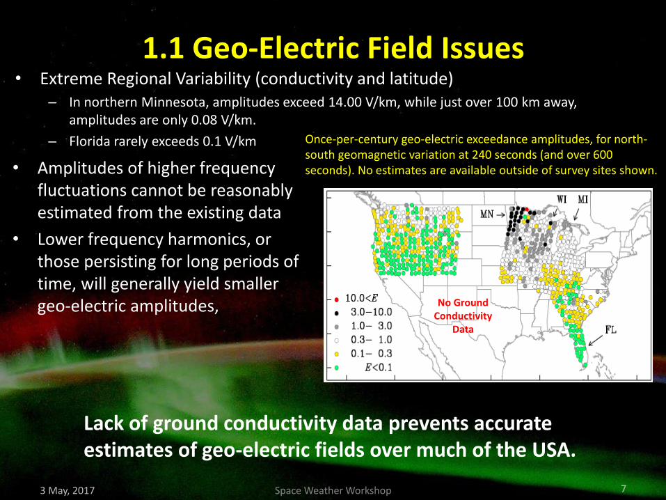
1.1 Geo-Electric Field Issues • Extreme Regional Variability (conductivity and latitude)

– In northern Minnesota, amplitudes exceed 14.00 V/km, while just over 100 km away, amplitudes are only 0.08 V/km.

– Florida rarely exceeds 0.1 V/km

3 May, 2017 7

Once-per-century geo-electric exceedance amplitudes, for north-south geomagnetic variation at 240 seconds (and over 600 seconds). No estimates are available outside of survey sites shown.

No Ground Conductivity

Data

• Amplitudes of higher frequency fluctuations cannot be reasonably estimated from the existing data

• Lower frequency harmonics, or those persisting for long periods of time, will generally yield smaller geo-electric amplitudes,

Lack of ground conductivity data prevents accurate estimates of geo-electric fields over much of the USA.

Space Weather Workshop

1.1 Geo-Electric Field

• Worst Case Observed: 14 V/km

– NERC Worst Case Guidance: 8 V/km

– March 89 (Quebec): 2 V/km

• Estimates of largest Geo-Electric fields will be highly location-dependent.


Benchmark 1.2 - Ionizing Radiation

• Solar Energetic Particles

– Sudden enhancements of electrons, protons, and heavy ions near Earth

• Radiation Belts

– Enhanced populations of electrons and protons surrounding Earth.

• Cosmic Rays

– Background population of fully ionized (no electrons) particles including all elements of the periodic table.

3 May, 2017 9

Estimates of extreme ionizing radiation will provide guidance for protecting for humans in space and in aviation and help satellite designers and operators mitigate impacts. Ionizing radiation also impact radio communication (Benchmark 1.3)

History of Proton Events


1.2 Ionizing Radiation

3 May, 2017 10

Solar proton event energy spectra for the statistical upper limit, plus one sigma.

Upper limit solar proton event energy spectra in LEO at an altitude of 400 km and spacecraft orbital angle of inclinations of 90, 70, 60 and 51.6 degrees.

10-hour polar exposure at altitude, based on the LaRC event proton spectrum for the Feb 56 SPE.

LEO GEO Aircraft

Radiation Belt worst case electron radiation belt flux estimates as a function of energy in GEO.

Radiation Belt worst-case fluxes versus energy are shown for two locations in HEO.

GEO HEO

For 1 in 100 year benchmark the force-field modulation was slightly more permissive than those approximated for current conditions.


SEPs

Radiation Belts Gallactic Cosmic Rays

1.2 Ionizing Radiation

• Solar Particles

• Cosmic Rays

• Radiation Belts

3 May, 2017 11

Solar Proton Event Integral Fluence (p/cm2) Energy (MeV) GEO LEO

400 km, 90o LEO

400 km, 70o LEO

400 km, 60o LEO

400 km, 51.6o 10 3.5 x 1010 6.9 x 109 4.1 x 109 1.7 x 109 5.2 x 107 30 1.3 x 1010 2.6 x 109 1.5 x 109 6.5 x 108 2.2 x 107

100 1.4 x 109 2.9 x 108 1.8 x 108 7.7 x 107 5.6 x 106 300 9.7 x 107 2.2 x 107 1.6 x 107 7.9 x 106 2.1 x 106

Differential GCR Flux (particles/cm2 sr s MeV/n) at 1 AU, = 200 MV Energy/nucleon Hydrogen Helium Carbon Oxygen Iron

10 MeV 1.3 x 104 1.7 x 105 6.1 x 107 5.3 x 107 1.2 x 107 30 MeV 3.2 x 104 3.7 x 105 1.3 x 106 1.1 x 106 2.5 x 107

100 MeV 5.3 x 104 4.7 x 105 1.7 x 106 1.5 x 106 2.9 x 107 300 MeV 4.1 x 104 2.7 x 105 9.9 x 107 8.9 x 107 1.5 x 107

1 GeV 1.2 x 104 6.9 x 106 2.6 x 107 2.4 x 107 3.7 x 108 30 GeV 1.7 x 105 8.1 x 107 3.3 x 108 3.0 x 108 4.9 x 109

100 GeV 1.2 x 106 5.4 x 108 2.4 x 109 2.1 x 109 3.9 x 1010 300 GeV 6.4 x 108 2.6 x 109 1.3 x 1010 1.1 x 1010 2.3 x 1011

1000 GeV 2.9 x 109 1.1 x 1010 6.2 x 1012 5.0 x 1012 1.2 x 1012

Location Energy Electrons (units = cm−2 s−1 sr−1) 1-in-100-Years Flux Most Extreme Fluxes Observed (date)

GEO (GOES-W)a

>2 MeV 7.68 x 105 4.92 x 105 (7/29/2004 - 1 in 50 yrs)

GEO (GOES-E)a >2 MeV 3.25 x 105 1.93 x 105 (7/29/2004 - 1 in 50 yrs) Upper Limit Flux (estimated) Most Extreme Fluxes Observed (date)

GEO (LANL)b 2.65 MeV 5.9 x 101 5.1 x 101 (7/30/2004) 625 keV 4.1 x 103 3.4 x 103 (7/29/2004) 270 keV 2.0 x 104 1.6 x 104 (6/5/1994)

HEO1 at L=4.0b >8.5 MeV 3.5 x 102 2.4 x 102 (8/30/1998) >4.0 MeV 4.5 x 104 2.6 x 104 (8/5/2004) >1.5 MeV 2.6 x 105 2.4 x 104 (8/30/1998)

HEO3 at L=6.0b >630 keV 1.0 x 105 6.0 x 104 (6/27/1998) at L=4.0 >630 keV 4.5 x 105 4.3 x 105 (8/29/1998) at L=2.25 >630 keV 2.1 x 105 1.9 x 105 (11/13/2004)

Estimates of 1 in 100 year flux levels for electrons estimated from the statistical AE9 reference model and scaled to GOES 2 MeV


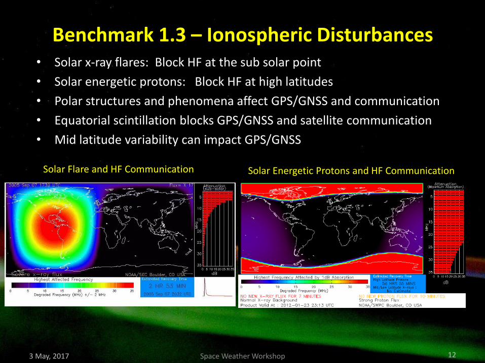
Benchmark 1.3 – Ionospheric Disturbances • Solar x-ray flares: Block HF at the sub solar point

• Solar energetic protons: Block HF at high latitudes

• Polar structures and phenomena affect GPS/GNSS and communication

• Equatorial scintillation blocks GPS/GNSS and satellite communication

• Mid latitude variability can impact GPS/GNSS

3 May, 2017 12

Solar Flare and HF Communication Solar Energetic Protons and HF Communication


• The state of the ionosphere has many dependencies. – Solar EUV irradiance

– Solar X-Ray irradiance

– Solar wind speed

– Solar wind density

– Interplanetary magnetic field

– Conditions in the magnetosphere

• Observations of large storms do not cover the full parameter space.

• Models of the ionosphere have not been tested and validated under extreme conditions.

• Estimates of extreme conditions within the ionosphere and the resulting impacts on technologies could have errors of an order of magnitude.

1.3 Ionospheric Disturbances Variability Issues and Geomagnetic Storm Impacts

13

– Solar EUV irradiance

– Solar X-Ray irradiance

– Solar wind speed

– Solar wind density

– Interplanetary magnetic field

– Conditions in the magnetosphere

Observed TEC on 16, 17, 18 March 2015

New Global TEC Product Developed by Fuller-Rowell and Fuller-Rowell Using COSMIC and Ground GPS data

3 May, 2017 Space Weather Workshop

1.3 Ionospheric Disturbances Phenome

non

Magnitude Location Event Duration Impact Technology Impact

Flare X-Class Flare

X- 28-40

Sunlit side

of Earth

D-Layer Enhancement Tens of

minutes

Radio waves absorbed in the

ionosphere up to 30 MHz

Loss of radar and communications

in HF and VHF frequencies up to

40-50 Mhz

Proton 30 MeV

Protons

1.2 x 109

/cm2 sec

High and

mid

latitudes

D-Layer Enhancement Several

days

Absorbs RF signals from HF to VHF

in the lower ionosphere

Loss of radar and communications

in HF and VHF frequencies up to

30-40 Mhz

Ge

om

agn

etic

Sto

rms

Kp 9+

High and

mid

latitudes

Polar Cap and Aurora 10s of

hours

Patches and plasma structures and

ionospheric gradients refract radio

waves

Degrades dual and single

frequency GPS accuracy. Possible

loss of signal lock

Kp 9+

Mid latitude

region on

dayside of

Earth

Traveling Ionospheric

Disturbances and Storm

Enhanced Densities

Hours Large TEC enhancements (up to 200

TEC units ) and strong gradients in

TEC. Large regions of ionospheric

depletion

Large GPS positioning errors

(>10x normal). Degrades OTH

radar performance. Loss of HF

frequencies

Latitudes

+/-20 degs

of geomag

equator.

Equatorial Scintillation A few

hours

after

sunset

Large scale plasma depletions and

associated small scale ionospheric

structures observed just after

sunset and generally up to

midnight. Scintillation of

transmitted radio signals.

Very large amplitude scintillations

of GPS signals. Phase

perturbations cause loss of signal

lock in dual frequency GPS

receivers. Possible total loss of HF

communication.

Improvements • Better estimates of extremes in the

input drivers • improved empirical and physics

based models • More analysis of existing data

3 May, 2017 Space Weather Workshop 14

1.4 Solar Radio Bursts

• Solar radio bursts are large enhancements in the solar noise produced by the sun usually associated with solar flares. They can affect a large range of radio frequencies and can last for 10s of minutes.

3 May, 2017 15

IGS – International GPS Service for Geodynamics

Peak Flux ~1.5x106 solar flux units (sfu)

1 sfu = 10-22 W m-2 Hz-1

30 minutes

VHF UHF GPS F10.7 Microwaves

0.03-0.3

GHz 0.3-3.0

GHz 1.176-1.602

GHz 2.8

GHz 4-20

GHz

• Solar Radio Bursts (SRB’s) interfere with radar, communication, and tracking signals.

• In severe cases, SRBs can inhibit the successful use of radio communications and disrupt a wide rage of systems reliant on PNT services (GPS/GNSS)

• Frequency bands for our benchmarks


1.4 Solar Radio Bursts

Freq. Bands (MHz)

Freq. Band Name

Nita Freq. Bands (MHz)

RSTN Discrete Freq. (MHz)

100 Yr. Benchmark (sfu*)

30-300 VHF 100-900 245 2.8x109

300-3000 UHF 1000-1700 410 610

1.2x107

1176-1602 GPS 1000-1700 1415 1.2x107

2800 F10.7 2000-3800 2695 1.3x107

4000-20000 Microwave 4900-7000 8400-11800 15000-37000

4995 8800 15400

3.7x107

Nita et al. 2002

Cumulative number of SRBs per day at frequencies > 2,000 MHz

1 in 100 years is a rate of 2.74x10-5 bursts/day

3 May, 2017 Space Weather Workshop 16

Estimating the Frequency of Events

1.5 Atmospheric Expansion Satellite Drag

• Understanding extremes in satellite drag will help satellite operators avoid collisions and debris during extreme events.

• Changes in neutral density impacts satellite orbit prediction and collision avoidance.

• Neutral density responds to thermospheric heating as a result of…

– Solar EUV (long term variability)

– Solar EUV (flares)

– Geomagnetic storms (CME’s)

• Additional Considerations:

– Winds are important and can change apparent drag by up to 25%

– Thermospheric structure is important.

• Benchmark includes neutral density/temperature, neutral winds (in-track and cross-track)

– At altitudes of 250 km, 400 km, and 850 km


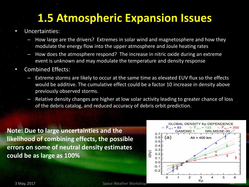
1.5 Atmospheric Expansion Issues • Uncertainties:

– How large are the drivers? Extremes in solar wind and magnetosphere and how they modulate the energy flow into the upper atmosphere and Joule heating rates

– How does the atmosphere respond? The increase in nitric oxide during an extreme event is unknown and may modulate the temperature and density response

• Combined Effects:

– Extreme storms are likely to occur at the same time as elevated EUV flux so the effects would be additive. The cumulative effect could be a factor 10 increase in density above previously observed storms.

– Relative density changes are higher at low solar activity leading to greater chance of loss of the debris catalog, and reduced accuracy of debris orbit prediction.

3 May, 2017 18

Note: Due to large uncertainties and the likelihood of combining effects, the possible errors on some of neutral density estimates could be as large as 100%


1.5 Atmospheric Expansion: Satellite Drag

3 May, 2017 19

Driver Parameter: Neutral Density

Percent Increase at Altitude relative to reference

250 km 400 km 850 km

Solar EUV* F10.7/F10.781 : 390/280 Ref: F10.7/F10.781 : 240/200

100-year 50% 100% 200%

Solar EUV* F10.7/F10.781 : 500/390 Ref: F10.7/F10.781 : 240/200

Theor. Max. 100% 160% 300%

Solar Flare X30 100-year - 75% -

Solar Flare X40 Theor. Max. - 135% -

Geomag. Storm** Ref: Halloween

100-year 400%

Combined: EUV, flare, CME

100-year 900%

* Reference model MSIS ** Reference model CTIPe


• Improvements – Better estimates of extremes in the input drivers – improved empirical and physics based models – Better drag coefficients in He atmosphere above 600 km.

Summary

• Initial benchmark assessments are complete

– Community feedback received.

• There are large uncertainties in several areas

• Uncertainties can be reduced and the Benchmarks refined with additional evaluation and model assessment.
