spacecraft formation dynamics and design

8/13/2019 Spacecraft Formation Dynamics and Design

http://slidepdf.com/reader/full/spacecraft-formation-dynamics-and-design 1/21



into the dynamics of the relative motion. However they cannot be used for actual mission design (althoughthere are some exceptions13). Indeed, they have inherent drawbacks: they neglect higher order terms in thedynamics and their domain of validity in phase space is very restricted and difficult to quantify. In addition,methods based on the state transition matrix tend to be valid only over short time spans. On the otherhand, numerical algorithms have been developed to design spacecraft formations using the true dynamics.Koon, Marsden, Masdemont and Murray14 use Routh reduction to reduce the dimensionality of the systemand then develop an algorithm based on the use of the Poincare map to find pseudo-periodic relative motionin the gravitational field of the Earth (including the J 2 gravity coefficient only), Xu and Fitz-Coy15 and

Avanzini, Biamonti and Minisci16 study formation maintenance as a solution to an optimal control problemthat they solve using a genetic algorithm and a multi-objective optimization algorithm respectively. Eventhough these methods use the exact dynamics and therefore can be used to solve a specific reconfigurationor formation maintenance problem, they fail (except14) to give insight on the dynamics. In addition, asnoticed by Wang and Hadaegh,17 formation reconfiguration design is a combinatorial problem. As a resultthe algorithms mentioned above are not appropriate for reconfiguration design as they require excessivecomputation (to reconfigure a formation of N spacecraft, there are N ! possibilities in general).

The method we expose in this paper directly tackles these issues and should be viewed as a semi-analyticapproach, since it consists of a numerical algorithm whose output is a polynomial approximation of thedynamics. As a consequence, we are able to use a very accurate dynamical model and to obtain tractableexpressions describing the relative motion. A fundamental difference with previous studies is that we describethe relative motion, i.e., the phase space in the vicinity of a reference trajectory, as two-point boundary valueproblems whereas it is usually described as an initial value problem. Such a description of the phase space isvery natural and convenient, for instance the reconfiguration problem and the search for periodic formationscan be naturally formulated as two-point boundary value problems.

In the present paper, to showcase the strength of our method, we have chosen to study two challengingmission designs.

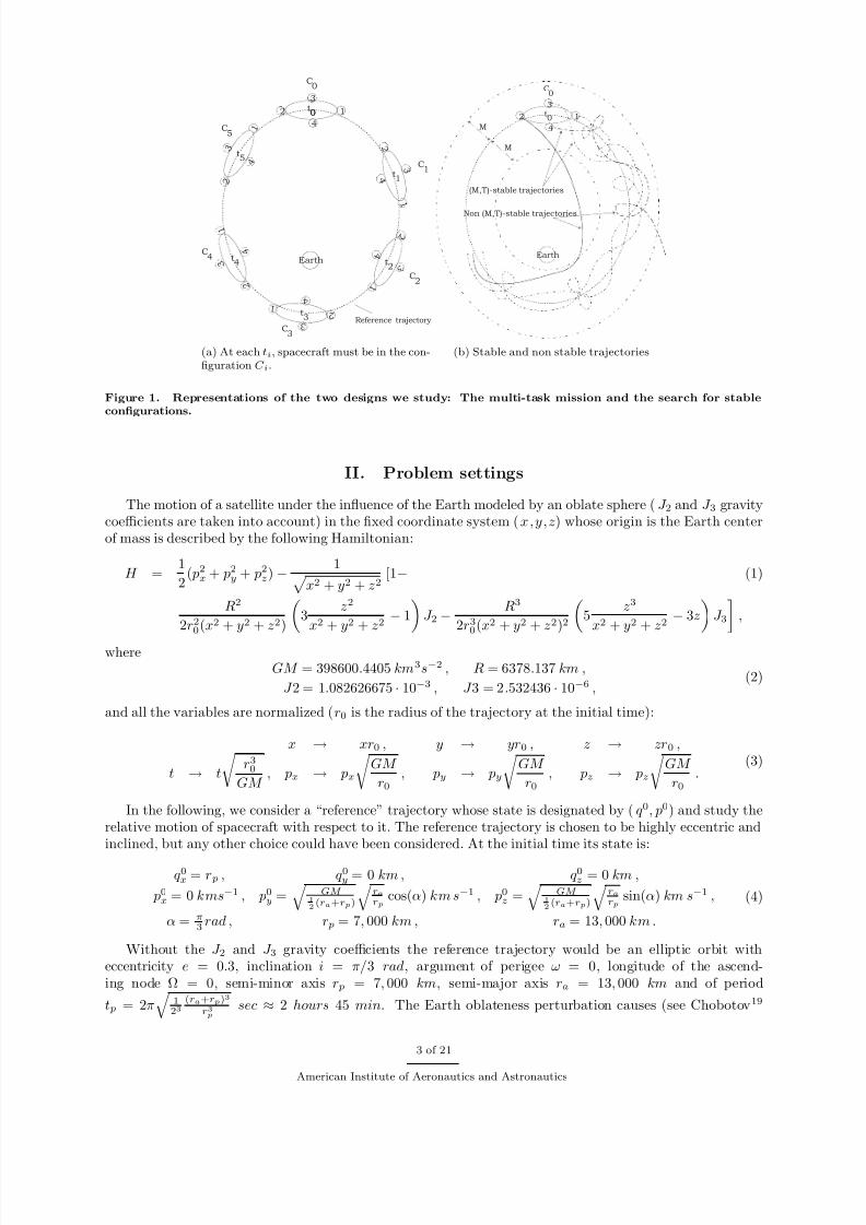
1. We first consider a spacecraft formation about an oblate Earth (the J 2 and J 3 gravity coefficientsare taken into account) that must achieve 5 missions over a one month period. For each mission theformation must be in a given configuration C i that has been specified beforehand, and we wish tominimize the overall fuel expenditure. The configurations C i are specified as relative positions of thespacecraft with respect to a specified reference trajectory (figure 1(a)). The C i’s may be fully definedor have one degree of freedom. In our example we require the spacecraft to be equally spaced on acircle centered on the reference trajectory at several epochs over the time period. The design of sucha mission has several challenges:

• The dynamics are non-trivial and non-integrable,

• the reference trajectory has high eccentricity, high inclination and is not periodic,

• missions are planned a month in advance,

• in our specific example discussed here, 4 spacecraft must achieve 5 missions, if one assumes thatthe C i are fully defined there are 7, 962, 624 ways of satisfying the missions,

• the C i may be defined by holonomic constraints and have an additional degree of freedom.

2. Next we consider two problems, the initial deployment of a formation and the redesign of an alreadydeployed formation. For both problems, given a reference trajectory we wish to place the spacecraftin its vicinity and ensure that they remain “close” to each other over an extended period of time (seefigure 1(b)). This design is also very challenging because:

• the dynamics and the reference trajectory are non-trivial (as before),

• trajectories must not collide (except at the initial time for the deployment problem),

• high accuracy in the initial conditions is required for long-term integration.

In the following, we first introduce the dynamical model as well as the reference trajectory. We thenbriefly recall the theory developed in18 for the solution of these problems. Finally, we study the missionsdiscussed above.

2 of 21

American Institute of Aeronautics and Astronautics



Earth

Reference trajectory

1

4

2

3

1

4

2

3

1

4

2

3

1 4

2

3

1

4

2

3

1

4

2

3

t00

t2

t5

t3

t4

t1

C0

C2

C1

C3

C4

C5

(a) At each ti, spacecraft must be in the con-figuration C i.

Earth

1

4

2

3t0

C0

(M,T)-stable trajectories

Non (M,T)-stable trajectories

M

M

(b) Stable and non stable trajectories

Figure 1. Representations of the two designs we study: The multi-task mission and the search for stable

configurations.

II. Problem settings

The motion of a satellite under the influence of the Earth modeled by an oblate sphere (J 2 and J 3 gravitycoefficients are taken into account) in the fixed coordinate system (x,y,z) whose origin is the Earth centerof mass is described by the following Hamiltonian:

H = 1

2( p2x + p2y + p2z) −

1 x2 + y2 + z2

[1− (1)

R2

2r20(x2 + y2 + z2)

3

z2

x2 + y2 + z2 − 1

J 2 −

R3

2r30(x2 + y2 + z2)2

5

z3

x2 + y2 + z2 − 3z

J 3

,

whereGM = 398600.4405 km3s−2 , R = 6378.137 km ,

J 2 = 1.082626675 · 10−3 , J 3 = 2.532436 · 10−6 ,(2)

and all the variables are normalized (r0 is the radius of the trajectory at the initial time):

x → xr0 , y → yr0 , z → zr0 ,

t → t

r30GM

, px → px

GM

r0, py → py

GM

r0, pz → pz

GM

r0.

(3)

In the following, we consider a “reference” trajectory whose state is designated by (q 0, p0) and study therelative motion of spacecraft with respect to it. The reference trajectory is chosen to be highly eccentric andinclined, but any other choice could have been considered. At the initial time its state is:

q 0x = r p , q 0y = 0 km , q 0z = 0 km ,

p0x = 0 kms−1 , p0y =

GM 12(ra+rp)

rarp

cos(α) km s−1 , p0z =

GM 12(ra+rp)

rarp

sin(α) km s−1 ,

α = π3 rad , r p = 7, 000 km , ra = 13, 000 km .

(4)

Without the J 2 and J 3 gravity coefficients the reference trajectory would be an elliptic orbit witheccentricity e = 0.3, inclination i = π/3 rad, argument of perigee ω = 0, longitude of the ascend-ing node Ω = 0, semi-minor axis r p = 7, 000 km, semi-major axis ra = 13, 000 km and of period

t p = 2π

123

(ra+rp)3

r3psec ≈ 2 hours 45 min. The Earth oblateness perturbation causes (see Chobotov19

3 of 21




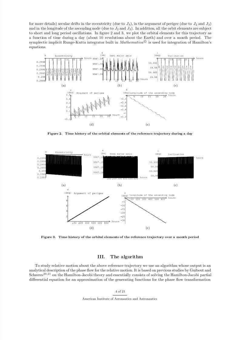
for more details) secular drifts in the eccentricity (due to J 3), in the argument of perigee (due to J 2 and J 3)and in the longitude of the ascending node (due to J 2 and J 3). In addition, all the orbit elements are subjectto short and long period oscillations. In figure 2 and 3, we plot the orbital elements for this trajectory asa function of time during a day (about 10 revolutions about the Earth) and over a month period. Thesymplectic implicit Runge-Kutta integrator built in Mathematica c is used for integration of Hamilton’sequations.

(a) (b) (c)

(d) (e)

Figure 2. Time history of the orbital elements of the reference trajectory during a day

100 200 300 400 500 600 hours

0.2986

0.2988

0.299

0.2992

0.2994

0.2996

0.2998

e Eccentricity

(a)

100 200 300 400 500 600 hours

9987.18

9987.18

9987.18

9987.18

a

km Semi major axis

(b)

100 200 300 400 500 600 hours

59.98

59.985

59.99

59.995

i

deg Inclination

(c)

(d) (e)

Figure 3. Time history of the orbital elements of the reference trajectory over a month period

III. The algorithm

To study relative motion about the above reference trajectory we use an algorithm whose output is ananalytical description of the phase flow for the relative motion. It is based on previous studies by Guibout andScheeres20,21 on the Hamilton-Jacobi theory and essentially consists of solving the Hamilton-Jacobi partialdifferential equation for an approximation of the generating functions for the phase flow transformation

4 of 21




describing the relative motion.

A. Relative motion

The relative motion of a spacecraft whose state is (q, p) moving in the Hamiltonian field defined by H (Eq.(2)) with respect to the reference trajectory (q 0(t), p0(t)) is described by the Hamiltonian function20 H h:

H

h

(X

h

, t) =

∞

p=2

p

i1,··· ,i2n=0i1+···+i2n= p

1

i1! · · · i2n!

∂ pH

∂q i11 · · ·∂q inn ∂pin+1

1 · · · ∂pi2nn (q

0

, p

0

, t)X

h

1

i1

. . . X

h

2n

i2n

, (5)

where X h = (∆q, ∆ p), ∆q = q −q 0, ∆ p = p− p0 and where we assume X h is small enough for the convergenceof the series. Let us truncate the series in Eq. (5) in order to keep terms of order at most N . Then wesay that the relative motion is described using an approximation of order N . Most past studies in theliterature (CW, improved CWa and Hill’s equations) consider an approximation of order 2, that is, a linearapproximation of the dynamics. Although such an approximation is useful to obtain a first picture of thedynamical environment as well as qualitative results, it cannot be used for designing an actual formation forseveral reasons. First, nonlinear effects are usually not negligible, especially over a long time span. Second,linear effects may not be dominant over a short time span even though the Taylor series b converges (see22

for a discussion on this issue). The algorithm we have developed tackles these issues, N must be finite butcan be as large as we want. There is no limit to the accuracy of the solution we obtain other than computer

memory (as we will see in the next section, if a solution up to order N − 1 is known, we need to solve (N +5)!N !5!

ordinary differential equations to obtain the N th order).

B. Solving boundary value problems

The design of spacecraft formations can often be reduced to solving boundary value problems. Indeed,the reconfiguration problem is a position to position boundary value problem,20 the search for periodicconfigurations, that is spacecraft configurations that repeat themselves over time, may also be treated as atwo-point boundary value problem23 and we will see in this paper how one may find stable formations, i.e.,formations for which spacecraft naturally stay close to each other for a long time, as a solution to boundaryvalue problems. Finally, if a maneuver is set up as an optimal control problem, the necessary conditions foroptimality can in many cases be reduced to a Hamiltonian system with known boundary values, that is, atwo-point boundary value problem.18,24

Traditionally used to analytically solve the equations of motion,25,26 the generating functions for thephase flow canonical transformation also allows one to solve two-point boundary value problems.21 Let usfirst consider a position q 0 to position q boundary value problem and recall the generating function of thefirst kind F 1(q, q 0, t):

pi = ∂F 1

∂q i(q, q 0, t) , (6)

p0i = −∂F 1∂q 0i

(q, q 0, t) , (7)

0 = H

q,

∂F 1∂q

, t

+

∂ F 1∂t

. (8)

Equation (8) is known as the Hamilton-Jacobi equation and allows us to solve for the generating functionF 1, whereas equations (6) and (7) solve the boundary value problem that consists in going from q 0 to q in tunits of time.

Now let us consider more general generating functions. Let (i1, · · · , i p)(i p+1, · · · , in) and (k1, · · · , kr)(kr+1, · · · , kn) be two partitions of the set (1, · · · , n) into two non-intersecting parts such that i1 < · · · < i p,

aas mentioned in the introduction the improved CW equations are the CW equations that take into account the J 2 gravitycoefficient.

bConsider for instance the converging Taylor series of (1 − t)x with respect to x. As t goes to 1, first terms are no moredominant.

5 of 21




i p+1 < · · · < in, k1 < · · · < kr and kr+1 < · · · < kn and define I p = (i1, · · · , i p), I p = (i p+1, · · · , in),K r = (k1, · · · , kr) and K r = (kr+1, · · · , kn). The generating function

F I p,K r(q I p , pI p , q 0Kr, p0 Kr

, t) = F (q i1 , · · · , q ip , pip+1, · · · , pin , q 0k1 , · · · , q 0kr , p0kr+1

, · · · , p0kn , t) (9)

verifies:

pI p = ∂F I p,K r

∂q I p(q I p , pI p , q 0Kr

, p0 Kr, t) , (10)

q I p = −∂F I p,K r

∂q I p(q I p , pI p , q 0Kr

, p0 Kr, t) , (11)

p0Kr = −

∂F I p,K r

∂q 0Kr

(q I p , pI p , q 0Kr, p0 Kr

, t) , (12)

q 0 Kr=

∂F I p,K r

∂p0 K r

(q I p , pI p , q 0Kr, p0 Kr

, t) , (13)

0 = H

q I p ,−

∂F I p,K r

∂pI p, ∂F I p,K r

∂q I p, pI p , t

+

∂ F I p,K r

∂t . (14)

Equation (14) is the general form of the Hamilton-Jacobi equation and allows one to solve for the

generating function F I p,K r . On the other hand, Eqs. (10), (11), (12) and (13) solve the boundary valueproblem that consists in going from (q I p , pI p) to (q 0Kr, p0 Kr

) in t units of time. Among the 4n generating

functions defined above, we can recover the 4 classical kinds of generating functions discussed by Goldstein;26

if the partitions are (1, · · · , n)() and ()(1, · · · , n) (i.e., p = n and r = 0) we recover the generating functionF 2. The case p = 0 and r = n corresponds to the generating function F 3 and if p = 0 and r = 0 we obtainF 4.

If the Hamiltonian in Eq. (14) is H h, as defined by Eq. (5), then the generating functions are associatedwith the phase flow that describes the relative motion and they solve relative boundary value problems. Interms of notation, (q 0, p0, q , p) becomes (∆q 0, ∆ p0, ∆q, ∆ p).

C. The numerics of the algorithm

There are two methods for finding the generating functions, one can either solve the Hamilton-Jacobi equation

(Eq. (14)) or use an indirect approach based on the initial value problem. These methods are detailed in22

and in the following we briefly review their characteristics. They both have their advantages and drawbacksand one usually needs to combine both of them. We will discuss this issue at the end of this section.

1. Solving the Hamilton-Jacobi equation

We assume the generating functions can be expressed as a Taylor series about the reference trajectory in itsspatial variables.

F I p,K r(y, t) =

∞q=2

qi1,··· ,i2n=0i1+···+i2n=q

1

i1! · · · i2n!f p,ri1,··· ,i2n

(t)yi11 · · · yi2n2n , (15)

where y = (∆q I p , ∆ pI p , ∆q 0Kr, ∆ p0 Kr

). We substitute this expression in Eq. (14), where H is the Hamilto-nian for the relative motion (Eq. 5). The resulting equation is an ordinary differential equation that has thefollowing structure:

P (y, f p,ri1,··· ,i2n(t), f p,ri1,··· ,i2n

(t)) = 0 , (16)

where P is a series in y with time dependent coefficients that are functions of f p,ri1,··· ,i2n(t), f p,ri1,··· ,i2n

(t).Equation (16) holds for all y if and only if all the coefficients of P are zero. In this manner, we transformthe ordinary differential equation (16) into a set of ordinary differential equations whose solutions are thecoefficients of the generating function F I p,K r . Now suppose that we have knowledge of the generating

functions up to order N − 1, then from Eq. (15) we deduce that we need to solve (N +5)!N !5! additional ordinary

differential equations to find order N .

6 of 21




This approach provides us with a closed form approximation of the generating functions. However, thereare inherent difficulties as generating functions may develop singularities which prevent the integration fromgoing further (see18,27,28 for more details on singularities). Techniques have been developed22 to bypassthis problem but have a cost in terms of computation. Typically, this method should only be used to solvegenerating functions over a short period of time.

2. The indirect approach

By definition, generating functions implicitly define the canonical transformation they are associated with.Hence, we may compute the generating functions from the canonical transformation, that is, compute thegenerating functions for the phase flow transformation from knowledge of the phase flow. In this section, wedevelop an algorithm based on these ideas (more details may be gleaned in22).

Recall Hamilton’s equations of motion for the relative motion: ∆q

∆ p

=

0 I n−I n 0

∇H h(∆q, ∆ p, t) . (17)

We suppose that ∆q (∆q 0, ∆ p0, t) and ∆ p(∆q 0, ∆ p0, t) can be expressed as series in the initial conditions(∆q 0, ∆ p0) with time dependent coefficients. We truncate the series to order N and insert these into Eq.(17). Hamilton’s equations reduce to a series in (∆q 0, ∆ p0) whose coefficients depend on the time dependentcoefficients and the derivatives of the series ∆q (∆q 0, ∆ p0, t) and ∆ p(∆q 0, ∆ p0, t). As in the previous section,we balance terms of the same order and transform Hamilton’s equations into a set of ordinary differentialequations whose variables are the time dependent coefficients defining ∆q and ∆ p as a series in ∆q 0 and∆ p0. Using ∆q (∆q 0, ∆ p0, t0) = ∆q 0 and ∆ p(∆q 0, ∆ p0, t0) = ∆ p0 as initial conditions for the integration, weare able to compute an approximation of order N for the phase flow. At linear order, this approach recoversthe state transition matrix. Then, a series inversion of the phase flow provides us with the gradient of thegenerating functions that can be integrated to find the generating functions.

The main advantage of this approach is that the phase flow is never singular, therefore the system of ordinary differential equations are always well-defined. However, this method requires us to solve moreequations than the previous methodc and provides us with the expression of the generating function at agiven time only (the time at which we perform the series inversion). In addition a symplectic algorithm shouldbe used to integrate the ordinary differential equations, otherwise we obtain an inconsistent expression of thegradient of the generating functions that cannot be integrated (some exactness conditions are not satisfied 29).

In this paper, we combine both methods, we first solve the initial value problem over a long time span usingthe symplectic implicit Runge-Kutta integrator built in M athematica c. Then we compute the generatingfunctions at a time of interest, say t1, and solve the Hamilton-Jacobi equation about t1, with initial conditionsequal to the values of the generating functions at t1 found using the indirect approach. For solving theHamilton-Jacobi equation, we use the M athematica c built in function N DSolve with its default attributesd.

IV. Formation design

In the previous sections we introduced a dynamical model, defined a reference trajectory and presented analgorithm whose outputs are the generating functions associated with the phase flow describing the relativemotion. We have also explained how these generating functions may be used to solve two-point boundaryvalue problems. We now combine all the above and use it to design spacecraft formations. We first use the“combined” algorithm to find the generating function F 1 up to order 4, that is we need to solve 203 ordinary

differential equations (see appendix for computational times). Once the generating functions are known, wecan solve any position to position boundary value problem with only six polynomial evaluations (Eqs. (6)and (7)).

cIf we want to find the generating function up to order N , then we need to solve 6N −1

k=1(k+5)!k!5!

equations, which is always

greater thanN

k=2(k+5)!k!5!

, the number of equations that need to be solved using the direct approach.dNDSolve switches between a non-stiff Adams method and a stiff Gear method and achieves a precision of 10−10.

7 of 21




A. Multi-task mission

We consider 4 imaging satellites flying in formation about the reference trajectory. We want to plan space-craft maneuvers over the next month knowing that they must observe the Earth, i.e., must be in a givenconfiguration C i at the following instants (chosen arbitrarily for our study):

t0 = 0 , t1 = 5 days 22 hours , t2 = 10 days 20 hours,

t3 = 16 days 2 hours , t4 = 21 days 14 hours , t5 = 26 days 20 hours.(18)

Define the local horizontal by the unit vectors (e1, e2) such that e2 is along r0×v0 and e1 is along e2×r0.At every ti, the configuration C i is defined by the four following relative positions (or slots):

q 1 = 700 m e1 , q 2 = −700 m e1 , q 3 = 700 m e2 , q 4 = −700 m e2 . (19)

Note that at ti, q 1 is in front of the reference state (in the local horizontal plane), q 2 is behind, q 3 is on theleft and q 4 is on the right (see figure 1(a)). At each ti, there must be one spacecraft per slot and we want todetermine the sequence of reconfigurations that minimizes the total fuel expendituree (other cost functionssuch as equal fuel consumption for each spacecraft may be considered as well). For the first mission, thereare 4! configurations (number of permutation of the set 1, 2, 3, 4). For the second mission, for each of theprevious 4! configurations, there are again 4! configurations, that is a total of 4!2 possibilities. Thus for 5missions there are 4!5 = 7, 962, 624 possible configurations.

In this paper, we focus on impulsive controls, but the method we develop can equivalently apply to

continuous thrust problems. Indeed, continuous thrust problems are usually solved using optimal controltheory and reduce to a set of necessary conditions that are formulated as a Hamiltonian two-point boundaryvalue problem. This boundary value problem can in turn be solved using the method we present in thispaper.24 Let us now design the above mission. We assume impulsive controls that consist of impulsivethrusts applied at ti∈[0,5]. For each of the four spacecraft, we need to compute the velocity at ti so that thespacecraft moves to its position specified at ti+1 under gravitational forces only. As a result, we must solve5 · 4! = 120 position to position boundary value problems (given two positions at ti and ti+1, we need tocompute the associated velocity). Using the generating functions, this problem can be handled at the costof only 720 function evaluations (computation times are given in the appendix). Then, we need to evaluatethe fuel expenditure (sum of the norm of all the required impulses, assuming zero relative velocities at theinitial and final times) for all the permutations (there are 7, 962, 624 combinations) to find the sequence thatminimizes the cost function. Figure 4 represents the number of configurations as a function of the valuesof the cost function. We notice that most of the configurations require at least three times more fuel than

the best configuration, and less than 6% yield values of the cost function that are less than twice the valueassociated with the best configuration. The cost function for the optimal sequence of reconfigurations is0.00644 km · s−1 whereas it is 0.0396 km · s−1 in the least optimal design. In the optimal case, the fourspacecraft have the following positions:

Spacecraft 1: (t0, q 1), (t1, q 2), (t2, q 2), (t3, q 2), (t4, q 2), (t5, q 2).Spacecraft 2: (t0, q 2), (t1, q 1), (t2, q 1), (t3, q 1), (t4, q 1), (t5, q 1).Spacecraft 3: (t0, q 3), (t1, q 4), (t2, q 4) (t3, q 4), (t4, q 3), (t5, q 4).Spacecraft 4: (t0, q 4), (t1, q 3), (t2, q 3) (t3, q 3), (t4, q 4), (t5, q 3).

whereas the worst scenario corresponds to:

Spacecraft 1: (t0, q 1), (t1, q 1), (t2, q 2), (t3, q 2), (t4, q 1), (t5, q 2).

Spacecraft 2: (t0, q 2), (t1, q 2), (t2, q 3), (t3, q 4), (t4, q 4), (t5, q 3).Spacecraft 3: (t0, q 3), (t1, q 3), (t2, q 1) (t3, q 3), (t4, q 3), (t5, q 4).Spacecraft 4: (t0, q 4), (t1, q 4), (t2, q 4) (t3, q 1), (t4, q 2), (t5, q 1).

We may verify, a posteriori , if the solutions found meet the mission goals, i.e., if the order 4 approximationof the dynamics is sufficient to simulate the true dynamics. Explicitly comparing the analytical solutionwith numerically integrated results shows that the spacecraft are at the desired positions at every ti with amaximum error of 1.5 · 10−8 km.

eEach impulses instantaneously change the velocity vector. The norm of this change quantifies the fuel expenditure

8 of 21




6.44 15.09 22.64 30.18 37.73

502,940

1,027,384

1,979,581

4,452,719*105

m/s

Figure 4. Number of configurations as a function of the value of the cost function

1. Considerations on collision management

Our algorithm does not consider the risk of collision in the design. However, it provides a simple way tocheck afterwards if there is collision. Recall the indirect method, it is based on the initial value problemand essentially consists in solving Hamilton’s equations for an approximation of the flow. Once such asolution is found, we can generate any trajectory at the cost of a function evaluation, there is no need tointegrate Hamilton’s equations again. Checking for collisions is again a combinatorial problem and thereforeour approach is particularly adapted to this. As an example let us verify if the design we proposed for themulti-task mission yields collisions. In figure 5 we plot the distance between each of the spacecraft. Weremark that only spacecraft 1 and 2, and spacecraft 3 and 4 may collide (relative distance less than 100 m).A detail of the figure shows that spacecraft 1 and 2 get as close as 40 meters after about 80 hours andspacecraft 3 and 4 may eventually collide.

(m)

(hours)

(a) Distance between Spacecraft 1 and2

(m)

(hours)

(b) Distance between Spacecraft 1 and3

(m)

(hours)

(c) Distance between Spacecraft 1 and4

(hours)

(m)

(d) Distance between Spacecraft 2 and3

(hours)

(m)

(e) Distance between Spacecraft 2 and3

(hours)

(m)

(f) Distance between Spacecraft 3 and4

Figure 5. Distance between the spacecraft as a function of time

It can be proven that for this specific mission, there is no design that prevents the relative motion of thespacecraft to be less than 100 m. In the best scenario, the smallest relative distance between the spacecraft

9 of 21




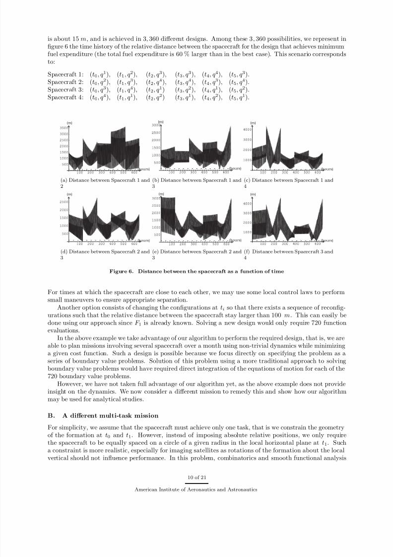
is about 15 m, and is achieved in 3, 360 different designs. Among these 3, 360 possibilities, we represent infigure 6 the time history of the relative distance between the spacecraft for the design that achieves minimumfuel expenditure (the total fuel expenditure is 60 % larger than in the best case). This scenario correspondsto:

Spacecraft 1: (t0, q 1), (t1, q 2), (t2, q 3), (t3, q 3), (t4, q 4), (t5, q 3).Spacecraft 2: (t0, q 2), (t1, q 3), (t2, q 4), (t3, q 4), (t4, q 3), (t5, q 4).Spacecraft 3: (t0, q 3), (t1, q 4), (t2, q 1) (t3, q 2), (t4, q 1), (t5, q 2).

Spacecraft 4: (t0, q 4), (t1, q 1), (t2, q 2) (t3, q 1), (t4, q 2), (t5, q 1).

(m)

(hours)

(a) Distance between Spacecraft 1 and2

(m)

(hours)

(b) Distance between Spacecraft 1 and3

(m)

(hours)

(c) Distance between Spacecraft 1 and4

(m)

(hours)

(d) Distance between Spacecraft 2 and3

(m)

(hours)

(e) Distance between Spacecraft 2 and3

(m)

(hours)

(f) Distance between Spacecraft 3 and4

Figure 6. Distance between the spacecraft as a function of time

For times at which the spacecraft are close to each other, we may use some local control laws to performsmall maneuvers to ensure appropriate separation.

Another option consists of changing the configurations at ti so that there exists a sequence of reconfig-urations such that the relative distance between the spacecraft stay larger than 100 m. This can easily bedone using our approach since F 1 is already known. Solving a new design would only require 720 functionevaluations.

In the above example we take advantage of our algorithm to perform the required design, that is, we areable to plan missions involving several spacecraft over a month using non-trivial dynamics while minimizinga given cost function. Such a design is possible because we focus directly on specifying the problem as aseries of boundary value problems. Solution of this problem using a more traditional approach to solvingboundary value problems would have required direct integration of the equations of motion for each of the720 boundary value problems.

However, we have not taken full advantage of our algorithm yet, as the above example does not provide

insight on the dynamics. We now consider a different mission to remedy this and show how our algorithmmay be used for analytical studies.

B. A different multi-task mission

For simplicity, we assume that the spacecraft must achieve only one task, that is we constrain the geometryof the formation at t0 and t1. However, instead of imposing absolute relative positions, we only requirethe spacecraft to be equally spaced on a circle of a given radius in the local horizontal plane at t1. Sucha constraint is more realistic, especially for imaging satellites as rotations of the formation about the localvertical should not influence performance. In this problem, combinatorics and smooth functional analysis

10 of 21




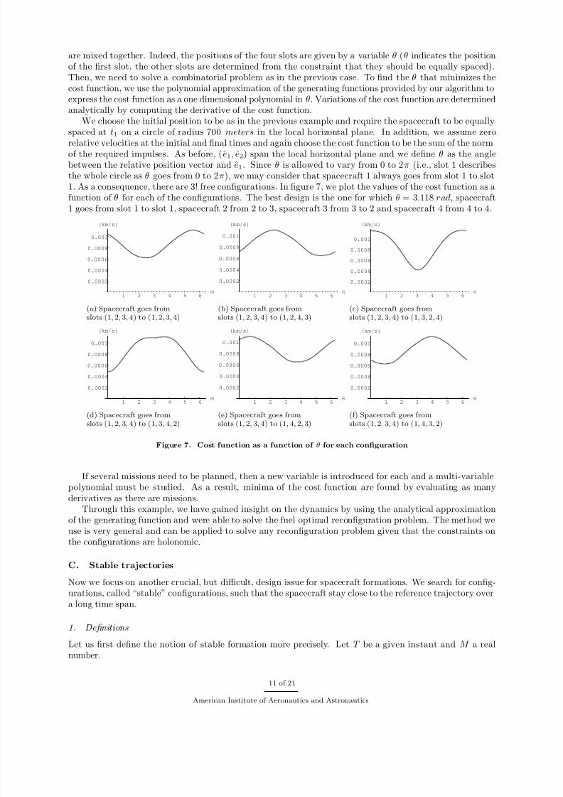
are mixed together. Indeed, the positions of the four slots are given by a variable θ (θ indicates the positionof the first slot, the other slots are determined from the constraint that they should be equally spaced).Then, we need to solve a combinatorial problem as in the previous case. To find the θ that minimizes thecost function, we use the polynomial approximation of the generating functions provided by our algorithm toexpress the cost function as a one dimensional polynomial in θ. Variations of the cost function are determinedanalytically by computing the derivative of the cost function.

We choose the initial position to be as in the previous example and require the spacecraft to be equallyspaced at t1 on a circle of radius 700 meters in the local horizontal plane. In addition, we assume zero

relative velocities at the initial and final times and again choose the cost function to be the sum of the normof the required impulses. As before, (e1, e2) span the local horizontal plane and we define θ as the anglebetween the relative position vector and e1. Since θ is allowed to vary from 0 to 2π (i.e., slot 1 describesthe whole circle as θ goes from 0 to 2π), we may consider that spacecraft 1 always goes from slot 1 to slot1. As a consequence, there are 3! free configurations. In figure 7, we plot the values of the cost function as afunction of θ for each of the configurations. The best design is the one for which θ = 3.118 rad, spacecraft1 goes from slot 1 to slot 1, spacecraft 2 from 2 to 3, spacecraft 3 from 3 to 2 and spacecraft 4 from 4 to 4.

1 2 3 4 5 6 Θ

0.0002

0.0004

0.0006

0.0008

0.001

kms

(a) Spacecraft goes fromslots (1, 2, 3, 4) to (1, 2, 3, 4)

1 2 3 4 5 6 Θ

0.0002

0.0004

0.0006

0.0008

0.001

kms

(b) Spacecraft goes fromslots (1, 2, 3, 4) to (1, 2, 4, 3)

1 2 3 4 5 6 Θ

0.0002

0.0004

0.0006

0.0008

0.001

kms

(c) Spacecraft goes fromslots (1, 2, 3, 4) to (1, 3, 2, 4)

1 2 3 4 5 6 Θ

0.0002

0.0004

0.0006

0.0008

0.001

kms

(d) Spacecraft goes fromslots (1, 2, 3, 4) to (1, 3, 4, 2)

1 2 3 4 5 6 Θ

0.0002

0.0004

0.0006

0.0008

0.001

kms

(e) Spacecraft goes fromslots (1, 2, 3, 4) to (1, 4, 2, 3)

1 2 3 4 5 6 Θ

0.0002

0.0004

0.0006

0.0008

0.001

kms

(f) Spacecraft goes fromslots (1, 2, 3, 4) to (1, 4, 3, 2)

Figure 7. Cost function as a function of θ for each configuration

If several missions need to be planned, then a new variable is introduced for each and a multi-variablepolynomial must be studied. As a result, minima of the cost function are found by evaluating as manyderivatives as there are missions.

Through this example, we have gained insight on the dynamics by using the analytical approximationof the generating function and were able to solve the fuel optimal reconfiguration problem. The method weuse is very general and can be applied to solve any reconfiguration problem given that the constraints onthe configurations are holonomic.

C. Stable trajectories

Now we focus on another crucial, but difficult, design issue for spacecraft formations. We search for config-urations, called “stable” configurations, such that the spacecraft stay close to the reference trajectory overa long time span.

1. Definitions

Let us first define the notion of stable formation more precisely. Let T be a given instant and M a realnumber.

11 of 21




Definition IV.1 (Stable relative trajectory). A relative trajectory between two spacecraft is (M, T )-stable if and only if their relative distance never exceeds M over the time span [0, T ].

Definition IV.2 (Stable formation). A formation of spacecraft is (M, T )-stable if and only if all thespacecraft have (M, T )-stable relative trajectories with respect to the reference trajectory.

Periodic formations are instances of stable formations, they are (M, ∞)-stable. We also point out thatour definition recovers the notion of Lyapunov stability: (M,∞)-stable relative trajectories are stable in thesense of Lyapunov. In this paper, we focus on (M, T )-stable formations with T large but finite, the approach

we present is not appropriate to find (M,∞)-stable configurations. However, when the reference trajectory isperiodic Guibout and Scheeres23 developed a technique based on generating functions and Hamilton-Jacobitheory to find periodic configurations.

2. Stable trajectories as solutions to two-point boundary value problems

In order to use the theory we have presented above, we formulate the search for stable trajectories astwo-point boundary value problems.

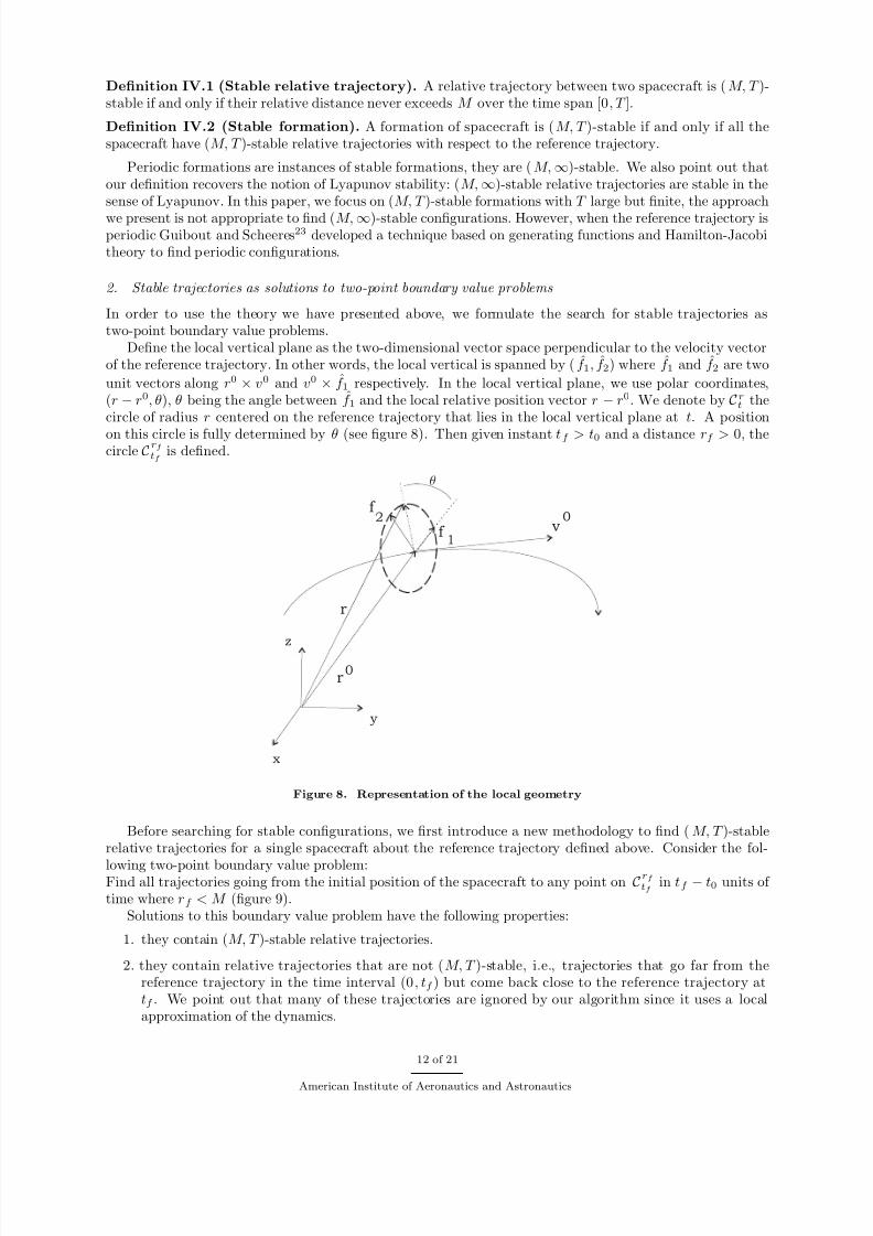
Define the local vertical plane as the two-dimensional vector space perpendicular to the velocity vectorof the reference trajectory. In other words, the local vertical is spanned by ( f 1, f 2) where f 1 and f 2 are two

unit vectors along r0 × v0 and v0 × f 1 respectively. In the local vertical plane, we use polar coordinates,(r − r0, θ), θ being the angle between f 1 and the local relative position vector r − r0. We denote by C rt thecircle of radius r centered on the reference trajectory that lies in the local vertical plane at t. A position

on this circle is fully determined by θ (see figure 8). Then given instant tf > t0 and a distance rf > 0, thecircle C

rf tf

is defined.

v0

x

y

z

r0

f 1

f 2

r

Figure 8. Representation of the local geometry

Before searching for stable configurations, we first introduce a new methodology to find ( M, T )-stablerelative trajectories for a single spacecraft about the reference trajectory defined above. Consider the fol-

lowing two-point boundary value problem:Find all trajectories going from the initial position of the spacecraft to any point on C

rf tf

in tf − t0 units of time where rf < M (figure 9).

Solutions to this boundary value problem have the following properties:

1. they contain (M, T )-stable relative trajectories.

2. they contain relative trajectories that are not (M, T )-stable, i.e., trajectories that go far from thereference trajectory in the time interval (0, tf ) but come back close to the reference trajectory attf . We point out that many of these trajectories are ignored by our algorithm since it uses a localapproximation of the dynamics.

12 of 21




v0f

1

f 2

f

tf

t0

q 0

Figure 9. Boundary value problem

On the other hand, we know that stable trajectories must have similar orbit elements as compared to thereference trajectory. Therefore, to discriminate between the solutions to the two-point boundary valueproblem we can use orbit elements, especially since we know, a priori , that the longitude of the ascendingnode and the argument of perigee have secular drifts. This leads us to define a cost function J as:

J = 14∆ωtf + 1

4∆ωtf − ∆ωt0 + 1

4∆Ωtf + 1

4∆Ωtf − ∆Ωt0 , (20)

where ∆ωtf corresponds to the relative argument of perigee at tf , i.e, the difference at tf between theargument of perigee of the spacecraft trajectory and the argument of perigee of the reference trajectory,∆ωtf − ∆ωt0 characterizes the change in the relative argument of perigee between t0 and tf and the otherterms are similar and involve the longitude of the ascending node instead.

Let us now consider the following boundary value problem: Find all trajectories going from the initialposition of the spacecraft to any point on C

rf tf

in tf − t0 units of time that minimize J .From the above discussion, we conclude that solutions to this boundary value problem characterize stable

relative trajectories.

3. Methodology

We showed in the previous section that the search for stable trajectories reduces to solving a two-pointboundary value problem while minimizing a given cost function. In this section, we solve this problem usingthe generating function theory introduced in the first part of this paper.

First we notice that F 1 solves the boundary value problem that consists of going from an initial positionq 0 to a position q f in tf units of time. Indeed, from Eqs. (6) and (7) we have:

p0 = −∂F 1∂q 0

(q, q 0, tf ) , (21)

pf = ∂F 1

∂q (q, q 0, tf ) . (22)

Then we assume that q f describes C rf tf

, that is, q f = rf cos(θf ) f 1 + rf sin(θf ) f 2 where θf ranges from 0 to

2π. Since F 1 is approximated by a polynomial in (q, q 0) with time-dependent coefficients, Eqs. (21) and (22)allow us to express p0 and pf as polynomials in θf with time-dependent coefficients. Finally, with knowledgeof p0(θf ), pf (θf ), q 0 and q f (θf ), we can express J as a function of θf and easily find its minima θ1f , · · · , θrf .

Stable trajectories are then those that travel from q 0 to q f = rf cos(θif ) f 1 + rf sin(θif )

f 2, i ∈ [1, r] in tf unitsof time.

4. Example

Let us illustrate this procedure by searching for stable trajectories for a spacecraft whose initial positionrelative to the reference trajectory is q 0 = (495,−428.6, 247.5) m in the inertial frame or equivalently q 0 =

13 of 21




700cos(π/4) f 1 +700sin(π/4) f 2 m. We use an order 4 approximation of the dynamics, tf = 10 d 19 h 13 minand rf = 700 m. Then, using a symbolic manipulator, we express J as a function of θf and plot its valuesin figure 10. It has two local minima at θ1 = 0.671503 rad and θ2 = 2.4006615 rad that correspond to stabletrajectories. The relative motions associated with these two trajectories are represented in figures 11 and12 over time spans smaller and larger than tf . We notice the excellent behavior of these trajectories, theyremain stable over a time interval larger than the one initially considered.

1 2 3 4 5 6 Θ rad

0.0001

0.0002

0.0003

Values of the cost functions

at t 259 h 13 min

Figure 10. Cost function as a function of θf

(a) x− y motion during 26 hours (b) x− z motion during 26 hours (c) y − z motion during 26 hours

(d) x − y motion during11 days 19 hours

(e) x − z motion during11 days 19 hours

(f) y − z motion during11 days 19 hours

(g) x − y motion during21 days 11 hours

(h) x − z motion during21 days 11 hours

(i) y − z motion during21 days 11 hours

Figure 11. Trajectory associated with the minimum θf = 0.671503 rad, tf = 10 d 19 h 13 min.

14 of 21




(a) x−y motion during 26 hours (b) x

−z motion during 26 hours (c) y

−z motion during 26 hours

(d) x − y motion during11 days 19 hours

(e) x − z motion during11 days 19 hours

(f) y − z motion during11 days 19 hours

(g) x − y motion during21 days 11 hours

(h) x − z motion during21 days 11 hours

(i) y − z motion during21 days 11 hours

Figure 12. Trajectory associated with the minimum θf = 2.4006615 rad, tf = 10 d 19 h 13 min.

Before going further, let us discuss the role played by tf . We transformed the search for stable trajectoriesinto a boundary value problem over a time span defined by tf that we apparently chose arbitrarily. By varyingtf , we notice that minima of the cost function correspond to different stable trajectories. In figure 13 we plotthe cost function as a function of θf for t = tf − 1 h 6 min = 10 d 18 h 19 min. In contrast to the previouscase, the cost function has only one minimum at θ = 3.814575 rad. In figure 14 we represent the trajectorythat corresponds to this minimum. It is stable but different from the previous ones (figures 11 and 12).This result was expected and makes our approach even more valuable. Indeed, since we reduced the searchfor stable trajectories to a boundary value problem, we completely ignore the behavior of the spacecraft atintermediary times t ∈ [0, tf ], we only take into account the states of the spacecraft at the initial time andat tf . As a result, short term oscillations play a major role and alter the locus of the minima of J . Thus, byvarying tf we are potentially able to find infinitely many stable trajectories going through q 0 at the initialtime. This aspect allows us to design a deployment problem, for instance, where several spacecraft are atthe same location at the initial time and we want to place them on stable trajectories that do not collide.

Furthermore, larger or smaller values of tf could have been chosen, however we must be aware that if tf is too small, short term oscillations may be as large as the drift and in that case the cost function does notdiscriminate well; its minima do not necessarily correspond to stable trajectories. On the other hand, if tf is very large, the minima correspond to (M, T )-stable relative trajectories with T increasing as tf increases.

Finally, in the above example we selected trajectories that correspond to minima of J and let tf vary tofind several stable trajectories. However, trajectories that correspond to values of J close to the minimum maybe stable trajectories as well. If we vary tf , say from T 1 to T 2, we noticed that the trajectory correspondingto the minimum of J at T 1 is different from the one corresponding to the minimum of J at T 2. Althoughthe trajectory associated to T 1 does not correspond to a minimum of J at T 2, it is stable and corresponds to

15 of 21




1 2 3 4 5 6 Θ rad

0.0001

0.0002

0.0003

0.0004

Values of the cost functions

at t 258 h 19 min

Figure 13. Cost function as a function of θf

(m)

(m)

(a) x− y motion during 26 hours

(m)

(m)

(b) x− z motion during 26 hours

(m)

(m)

(c) y − z motion during 26 hours

Figure 14. Trajectory associated with the minimum θ =f 3.814575 rad, tf = 10 d 18 h 19 min.

a small value of J at T 2. As a result, we are able to identify regions in which there are no stable trajectorythat go through an initial position q 0 and through the circle of radius rf at tf . For example, all stable

trajectories that goes through q 0 = (495,−428.6, 247.5) m and q f = 700 cos(θf ) f 1 + 700 sin(θf ) f 2 m at tf are localized on the arc defined by θf ∈ [0, π] when tf = 10 d 19 h 13 min and by θf ∈ [2, 5] rad whentf = 10 d 18 h 19 min.

D. Stable configurations

In this section, we generalize the approach introduced above in order to design stable configurations. Withoutloss of generality, and for sake of simplicity, we assume that the formation is on C r0t0 at the initial time so that

the positions of the spacecraft are determined by the angle θ0, the angle between f 1 and the local relativeposition vector. As a result, the initial position may be regarded as a function of θ0. Thus, Eqs. (21) and(22) provide a polynomial approximation of p0 and pf in the variables (θ0, θf ) (instead of θf only) withtime-dependent coefficients. The procedure to find stable trajectories is the same as before but now we havean additional variable, θ0. In figure 15 we represent the values of the cost function as a function of θi andθf for different times. We notice that if two out of the three variables (θf , θ0, tf ) are given, there exists avalue of the third variable that minimizes the cost function. In other words, whatever θ

0 and t

f are, there

exists a stable trajectory that goes through the initial position at the initial time and reaches C rf tf in tf units

of time. Moreover, if tf varies, minima of the cost function correspond to different stable trajectories due toshort term oscillations.

1. Example

We consider a formation of 4 spacecraft equally spaced on a circle of radius 700 m about the referencetrajectory that lies in the local vertical plane at the initial time. Spacecraft k has its initial position definedby θi = π/4 + (k − 1)π/2. Stable trajectories may be found by minimizing the cost function with respect to

16 of 21




(a) At tf = 10 d 18 h 19 min (b) At tf = 10 d 18 h 34 min (c) At tf = 10 d 18 h 42 min

(d) At tf = 10 d 18 h 50 min (e) At tf = 10 d 18 h 57 min (f) At tf = 10 d 19 h 13 min

Figure 15. Cost function as a function of the initial and final positions for several tf

θ. For every choice of tf there is a solution to the minimization problem (see figure 15). As a result, we areable to find infinitely many stable trajectories for each spacecraft. In figure 16 we plot the trajectories of thefour spacecraft that are found by considering tf = 10 d 18 h 19 m and in figure 17, tf = 10 d 19 h 13 m. Thetwo solutions have very different properties; Even though the positions at the final time tf are constrainedto be at 700 m from the reference trajectory in the local vertical plane, the relative distance may be largeat intermediary times. For instance the solution found for tf = 10 d 18 h 19 m yields a formation that is aslarge as 6 km. Such trajectories cannot be found using linear approximations of the relative motion.

V. Conclusions

In this paper, we have joined elements of Hamilton-Jacobi theory and a robust algorithm that computesgenerating functions to address the challenges that arise in missions involving spacecraft flying in formation.Despite a complex dynamical model and an arbitrary reference trajectory we have been able to obtain asemi-analytic description of the phase flow as two-point boundary value problems. Such a description of thephase space is superior in many ways to the traditional approach based on the initial value problem. Inparticular it allows us to solve two-point boundary value problems using only simple functions evaluations.This aspect is crucial when dealing with spacecraft formations because of the combinatorial nature of thereconfiguration problem. In addition, we have shown that the algorithm we have developed is able to predictthe dynamics over a long time span with high accuracy. The examples we have chosen illustrate the use of our method, but our method does not reduce to these examples and can be used to deal with more complexproblems. To conclude, we recall the main feature of our method:

• The dynamical environment may be as complex as one wants, the only constraint being that thedynamical system must be Hamiltonian. In addition, the complexity of the dynamical system does notseriously impact the computation times.

• The reference trajectory may be arbitrary, however it influences the domain of convergence of the seriesdefining H h. Techniques to estimate this domain have been developed by Guibout and Scheeres.21

• The time span we consider may be very large, the larger it is the longer the ordinary differentialequations obtained with the indirect algorithm should be integrated. The main advantage of describingthe phase flow as two-point boundary value problems is that the time period we consider does not

17 of 21




influence the accuracy of the results. This aspect is of main importance, especially as this is a weaknessof traditional approaches based on the initial value problem.

• Our approach also allows one to deal with low-thrust spacecraft. In this case, the reconfigurationproblem can be formulated as an optimal control problem whose necessary conditions for optimalityare a Hamiltonian two-point boundary value problem. For these problems, the dynamical environmentmay not be Hamiltonian since the necessary conditions for optimality yield a Hamiltonian system.However, it should be emphasized that the dimensionality is double (because of the adjoint variables).

• There are no limitation on the complexity of the formation geometry in the reconfiguration problemas long as the geometry can be described with constraints on (q, p) only.

• From the semi-analytic expression of the generating functions, several problems may be addressed. Wehave seen how to solve the reconfiguration problem and the deployment problem, we have also beenable to find stable configurations and in previous articles the authors showed that one can also findperiodic configurations. In the future, additional problems will be addressed.

Finally, the M athematica c package we have developed to run these simulations is freely available from theauthors upon request.

Acknowledgement

The work described here was funded in part by NASA’s Office of Space Science and by the Interplan-etary Network Technology Program by a grant from the Jet Propulsion Laboratory, California Institute of Technology which is under contract with the National Aeronautics and Space Administration.

A. Appendix: Computational times

All the computations have been made using M athematica c 5.0 on a 2GHz processor with 2GB RAMrunning under Linux.

• Computation of the generating function F 1 up to order 4 over a time span of about 5 days: about 5hours.

• Solving the 120 two-point boundary value problems in the first multi-task missions: about 3 minutes.

• Solving the second multi-task mission: about 1 minute.

• Solving the deployment problem: instantaneous once F 1 is known.

• Finding stable configurations: instantaneous once F 1 is known.

References

1Hope, A. S. and Trask, A. J., “Pulsed thrust method for hover formation flying,” AAS/AIAA Astrodynamics Specialist Conference and Exhibit, Big Sky, Montana. Paper AAS 03-655 , AAS, 2003.

2Vadali, S., Vaddi, S., and Alfriend, K., “An intelligent control concept for formation flying satellite constellations,”International journal of robust and nonlinear control , Vol. 12, No. 2-3, 2002, pp. 97–115.

3Gurfil, P. and Kasdin, N. J., “Nonlinear Modeling and Control of Spacecraft Formation Dynamics in the Configuration

Space,” Submitted to the Journal of Guidance, Control and Dynamics , 2002.4Scheeres, D., Hsiao, F., and Vinh, N., “Stabilizing motion relative to an unstable orbit: Applications to spacecraftformation flight,” Journal of Guidance, Control, and Dynamics, Vol. 26, No. 1, 2003, pp. 62–73.

5Howell, K. and Marchand, B., “Control Strategies for Formation Flight in the Vicinity of a Libration Point Orbit,” AIAA13th AAS/AIAA Space Flight Mechanics Meeting, Ponce, Puerto Rico, AAS Paper No. 03-113 , 2003.

6Vadali, S., Bae, H., and Alfriend, K. T., “Control of Libration Point Satellite Formations,” 14th Space Flight MechanicsMeeting, Maui, Hawaii, AAS Paper No. 034-161 , 2004.

7Vaddi, S. S., Alfriend, K. T., and Vadali, S. R., “Sub-optimal formation establishment and reconfiguration using impulsivethrust,” AAS/AIAA Astrodynamics Specialist Conference and Exhibit, Big Sky, Montana. Paper AAS 03-590 , AAS, 2003.

8Alfriend, K. and Schaub, H., “Dynamics and control of spacecraft formations: challenges and some solutions,” AAS/AIAAAstrodynamics Specialist Conference and Exhibit, College Station, Texas. Paper AAS 00-259 , AAS, 2000.

18 of 21




9Lovell, T., Horneman, K., Tollefson, M., and Tragesser, S., “A guidance algorithm for formation reconfiguration andmaintenance based on perturbed Clohessy-Wiltshire equations,” AIAA/AAS Astrodynamics Specialist Conference and Exhibit,Big Sky, Montana. Paper AAS 03-649 , AAS, 2003.

10Hsiao, F. and Scheeres, D., “Design of Spacecraft Formation Orbits Relative to a Stabilized Trajectory,” AAS/AIAASpace Flight Mechanics meeting, Ponce, Puerto Rico. Paper AAS 03-175 , AAS, 2003.

11Hussein, I., Scheeres, D., and Hyland, D., “Control of a Satellite Formation For Imaging Applications,” American Control Conference, Denver, Colorado, AAS, 2003.

12Mishne, D., “Maintaining periodic relative trajectories of satellite Formation by using power-limited thrusters,”AAS/AIAA Astrodynamics Specialist Conference and Exhibit, Big Sky, Montana. Paper AAS 03-656 , AAS, 2003.

13

Alfriend, K. T., Vaddi, S. S., and Lovell, T. A., “Formation maintenance for low Earth near-circular orbits,” AAS/AIAAAstrodynamics Specialist Conference and Exhibit, Big Sky, Montana. Paper AAS 03-652 , AAS, 2003.14Koon, W., Marsden, J., Masdemont, J., and Murray, R., “J 2 dynamics and formation flight,” AIAA Guidance, Naviga-

tion, and Control Conference, Montreal, Canada, August, AIAA 2001-4090 , AIAA, 2001.15Xu, Y. and Fitz-Coy, N., “Genetic algorithm based sliding method control in the leader / follower satellites pair mainte-

nance,” AAS/AIAA Astrodynamics Specialist Conference and Exhibit, Big Sky, Montana. Paper AAS 03-648 , AAS, 2003.16Avanzini, G., Biamonti, D., and Minisci, E. A., “Minimum-fuel/minimum-time maneuvers of formation flying satellites,”

AAS/AIAA Astrodynamics Specialist Conference and Exhibit, Big Sky, Montana. Paper AAS 03-654 , AAS, 2003.17Wang, P. K. C. and Hadaegh, F. Y., “Minimum-fuel formation reconfiguration of multiple free-flying spacecraft,” The

Journal of the Astronautical Sciences, Vol. 47, No. 1-2, 1999, pp. 77–102.18Guibout, V. M. and Scheeres, D. J., “Solving two-point boundary value problems using generating functions: Theory

and Applications to optimal control and the study of Hamiltonian dynamical systems,” Submitted to the Journal of nonlinear science , 2004.

19Chobotov, V. A., Orbital mechanics, American Institute of Aeronautics and Astronautics, 3rd ed., 2003.20Guibout, V. M. and Scheeres, D. J., “Formation Flight with generating functions: Solving the relative boundary value

problem,” AIAA/AAS Astrodynamics Specialist Conference and Exhibit, Monterey, California. Paper AIAA 2002-4639 , AIAA,2002.

21Guibout, V. M. and Scheeres, D. J., “Solving relative two-point boundary value problems: Spacecraft formation flighttransfers application,” AIAA, Journal of Control, Guidance and Dynamics , Vol. 27, No. 4, 2003, pp. 693–704.

22Guibout, V. M. and Scheeres, D. J., “An algorithm that solves the Hamilton-Jacobi equation,” In preparation , 2004.23Guibout, V. M. and Scheeres, D. J., “Periodic orbits from generating functions,” AAS/AIAA Astrodynamics Specialist

Conference and Exhibit, Big Sky, Montana. Paper AAS 03-566 , AAS, 2003.24Scheeres, D. J., Park, C., and Guibout, V. M., “Solving optimal control problems with generating functions,” AAS/AIAA

Astrodynamics Specialist Conference and Exhibit, Big Sky, Montana. Paper AAS 03-575 , AAS, 2003.25Greenwood, D. T., Classical Dynamics , Prentice-Hall, 1977.26Goldstein, H., Classical Mechanics, Addison-Wesley, 2nd ed., 1980.27Arnold, V. I., Mathematical Methods of Classical Mechanics, Springer-Verlag, 2nd ed., 1988.28Abraham, R. and Marsden, J. E., Foundations of mechanics, W. A. Benjamin, 2nd ed., 1978.29Guibout, V. and Bloch, A., “Discrete variational principles and Hamilton-Jacobi theory for mechanical systems and

optimal control problems,” Physica D, submitted , 2004.

19 of 21




(m)

(m)

(a) Spacecraft 1

(m)

(m)

(b) Spacecraft 1

(m)

(m)

(c) Spacecraft 1

(m)

(m)

(d) Spacecraft 2

(m)

(m)

(e) Spacecraft 2

(m)

(m)

(f) Spacecraft 2

(m)

(m)

(g) Spacecraft 3

(m)

(m)

(h) Spacecraft 3

(m)

(m)

(i) Spacecraft 3

(m)

(m)

(j) Spacecraft 4

(m)

(m)

(k) Spacecraft 4

(m)

(m)

(l) Spacecraft 4

Figure 16. Trajectories of the four spacecraft found by minimizing the cost function at tf = 10 d 18 h 19 m

20 of 21




(m)

(m)

(a) Spacecraft 1

(m)

(m)

(b) Spacecraft 1

(m)

(m)

(c) Spacecraft 1

(m)

(m)

(d) Spacecraft 2

(m)

(m)

(e) Spacecraft 2

(m)

(m)

(f) Spacecraft 2

(m)

(m)

(g) Spacecraft 3

(m)

(m)

(h) Spacecraft 3

(m)

(m)

(i) Spacecraft 3

(m)

(m)

(j) Spacecraft 4

(m)

(m)

(k) Spacecraft 4

(m)

(m)

(l) Spacecraft 4

Figure 17. Trajectories of the four spacecraft found by minimizing the cost function at tf = 10 d 19 h 13 m

spacecraft formation dynamics and design

Documents