spacial analysis of foreclosure and neighborhood
TRANSCRIPT

University of Northern Iowa University of Northern Iowa
UNI ScholarWorks UNI ScholarWorks
Dissertations and Theses @ UNI Student Work
2015
Spacial analysis of foreclosure and neighborhood characteristics Spacial analysis of foreclosure and neighborhood characteristics
in Miami metropolitan area, Florida in Miami metropolitan area, Florida
Adejoh Emmanuel Ogbe University of Northern Iowa
Let us know how access to this document benefits you
Copyright ©2015 Adejoh Emmanuel Ogbe
Follow this and additional works at: https://scholarworks.uni.edu/etd
Part of the Human Geography Commons, and the Real Estate Commons
Recommended Citation Recommended Citation Ogbe, Adejoh Emmanuel, "Spacial analysis of foreclosure and neighborhood characteristics in Miami metropolitan area, Florida" (2015). Dissertations and Theses @ UNI. 178. https://scholarworks.uni.edu/etd/178
This Open Access Thesis is brought to you for free and open access by the Student Work at UNI ScholarWorks. It has been accepted for inclusion in Dissertations and Theses @ UNI by an authorized administrator of UNI ScholarWorks. For more information, please contact [email protected].

SPATIAL ANALYSIS OF FORECLOSURE AND NEIGHBORHOOD
CHARACTERISTICS IN MIAMI METROPOLITAN AREA, FLORIDA
An Abstract of a Thesis
Submitted
in Partial Fulfillment
of the Requirements for the Degree
Master of Arts
Adejoh Emmanuel Ogbe
University of Northern Iowa
May, 2015

ABSTRACT
In 2013, the State of Florida had 13 of the top 20 metropolitan statistical areas (MSA)
with the highest foreclosure rate in the country. Despite the high ranking, extensive
research on foreclosure has yet to be carried out within the Miami-Fort Lauderdale-
Pompano Beach MSA. This research is a foray into an uncharted territory to understand
the relationship between foreclosure and neighborhood characteristics in the Miami
metropolitan area (MMA) within Miami-Dade County. The study was conducted in two
phases: The first phase was to identify the foreclosure pattern in the MMA from 2010-
2013 by implementing the use of spatial analysis such as nearest neighbor analysis,
spatial autocorrelation, and cluster and outlier analysis. The statistical analysis used also
included correlation analysis, principal component analysis, and regression analysis. The
dataset used contained foreclosure count from 2010-2013 and the 2010 census tract level
data on neighborhood characteristics such as ethnicity and racial compositions,
socioeconomic, demographic, and housing. The spatial and statistical analysis carried out
was used to identify the relationship between foreclosure and the neighborhood
characteristics. The second phase studied the effect of foreclosure on crime in the city of
Miami. Crime data from 2011-2012 was used to study the relationship between crime,
foreclosure, and the above mentioned neighborhood characteristics. The statistical
analysis carried out in this phase included correlation analysis and regression analysis.
Results of the study showed that in MMA, the relationship between foreclosure and other
neighborhood characteristics was insignificant. However, the result for the spatial pattern
of foreclosure in MMA showed that houses of similar market values were clustered in the

northeastern, southeastern and central areas. Additionally, areas dominated by the
African American population showed low economic activity and high foreclosure
concentration compared to other areas, which could be an influence of subprime lending.
Finally, foreclosure alone had no impact on crime whatsoever, but vacancy rate was
statistically significant to property crime in the city of Miami. These findings are
important in understanding foreclosure distribution and clustering patterns in MMA

SPATIAL ANALYSIS OF FORECLOSURE AND NEIGHBORHOOD
CHARACTERISTICS IN MIAMI METROPOLITAN AREA, FLORIDA
A Thesis
Submitted
in Partial Fulfillment
of the Requirements for the Degree
Master of Arts
Adejoh Emmanuel Ogbe
University of Northern Iowa
May, 2015

ii
This Study by: Adejoh Emmanuel Ogbe
Entitled: Spatial Analysis of Foreclosure and Neighborhood Characteristics in Miami
Metropolitan Area, Florida
Has been approved as meeting the thesis requirement for the
Degree of Masters of Arts in Geography
___________ _____________________________________________________
Date Dr. Bingqing Liang, Chair, Thesis Committee
___________ _____________________________________________________
Date Dr. Andrey N. Petrov, Thesis Committee Member
___________ _____________________________________________________
Date Dr. Alex P. Oberle, Thesis Committee Member
________ _____________________________________________________
Date Dr. Benjamin Keith Crew, Thesis Committee Member
___________ _____________________________________________________
Date Dr. April Chatham-Carpenter, Interim Dean, Graduate College

iii
I dedicate this thesis to my mother.
Whatever I have achieved today is because
of her unwavering faith in me. She always
provides the best of everything I ask for.

iv
ACKNOWLEDGMENTS
First of all I would like to thank the Almighty God for granting me the wisdom,
strength, and fortitude to persevere all through my Master’s program.
Secondly, I would like to express my utmost gratitude to my family that are thousands
of miles away but still made me feel like they were right next to me. For the love,
support, and encouragement you gave me I am eternally grateful. To John and Margie
Kaiser who welcomed me into their family and treated me like one of their own, I am
grateful for the unquantifiable support throughout the years.
To Dr. Bingqing Liang, my advisor who has been the guiding light in my path to
achieving academic excellence, I say thank you for all the guidance, support, and
constructive criticism you have given me. I would not have been able to complete this
thesis without the intellectual input, advice, and direction of my committee members: Dr.
Andrey Petrov, Dr. Alex Oberle, and Dr. Keith Crew. Reverence is also given to Mr.
John Degroote, Dr. Patrick Pease, Dr. Tim Strauss, Dr. J. Henry Owusu, Mr. Chris Essig,
and Mr. Mark Jacobson. You all have in more ways than one contributed in impacting
knowledge unto me over the years, and for that I am eternally grateful. I would also like
to thank the UNI Department of Geography, and the College of Social and Behavioral
Sciences (CSBS) for the financial support provided to assist in purchasing the data used
in this study.

v
Finally, I would like to thank my friends, most especially our little Nigerian
community here at Cedar Falls who helped me keep my sanity when things were not
going according to plan, I love and appreciate you all for been there when it counted the
most.

vi
TABLE OF CONTENTS
PAGE
LIST OF TABLES ............................................................................................................. ix
LIST OF FIGURES .............................................................................................................x
CHAPTER 1 INTRODUCTION .........................................................................................1
1.1 Introduction .............................................................................................................1
1.2 Research Background ..............................................................................................1
1.3 Knowledge Gap .......................................................................................................5
1.4 Purpose and Objective of Study .............................................................................10
1.5 Significance of Study .............................................................................................11
1.6 Structure of the Thesis ...........................................................................................12
CHAPTER 2 LITERATURE REVIEW ............................................................................13
2.1 Introduction ............................................................................................................13
2.2 Foreclosure Causal Factors in the United States ....................................................13
2.3 Methodological Approaches to Foreclosure Studies .............................................17
2.4 Using GIS to Study Foreclosure Pattern ................................................................19
2.5 Conclusion .............................................................................................................20
CHAPTER 3 STUDY AREA AND METHODOLOGY ..................................................21
3.1 Introduction ............................................................................................................21
3.2 Study Area .............................................................................................................21
3.3 Methodology .........................................................................................................24

vii
3.3.1 Data Sets .......................................................................................................24
1 Foreclosure data ............................................................................................25
2 Crime data .....................................................................................................25
3 Socioeconomic and housing data ..................................................................25
4 USPS vacant houses data ..............................................................................26
3.3.2 Software ........................................................................................................26
3.3.3 Data Preparation ...........................................................................................26
3.3.4 Spatial Analysis of foreclosure in MMA ......................................................31
1 Nearest neighbor analysis .............................................................................32
2 Spatial autocorrelation ..................................................................................32
3 Cluster and outlier analysis ...........................................................................33
3.3.5 Statistical Analysis of foreclosure in MMA and the city of Miami ..............33
1 Correlation analysis ......................................................................................33
2 Principal component analysis .......................................................................33
3 Regression analysis .......................................................................................34
CHAPTER 4 RESULTS ....................................................................................................36
4.1 Introduction ............................................................................................................36
4.2 Nearest Neighbor Analysis Result for Foreclosure in MMA ................................36
4.3 Spatial autocorrelation Result for Foreclosure in MMA .......................................36
4.4 Cluster and Outlier Analysis Results for Foreclosure in MMA ............................37
4.5 Correlation Analysis Result ...................................................................................43
4.6 Principal Component Analysis Result ...................................................................46

viii
4.6.1 Economic Indicator ......................................................................................50
4.6.2 Crowdedness Indicator ..................................................................................52
4.6.3 Racial Diversity Indicator .............................................................................53
4.7 Results on the Regression Analysis for Foreclosure in MMA ..............................55
4.8 Sample Study on the Northern African American Population in MMA ...............57
4.9 Results on the Correlation and Regression Analysis for the City of Miami ..........64
CHAPTER 5 DISCUSSIONS ...........................................................................................70
5.1 Introduction ............................................................................................................70
5.2 Foreclosure and Neighborhood Characteristics in MMA .....................................70
5.3 Foreclosure and Crime in the City of Miami .........................................................76
CHAPTER 6 CONCLUSIONS .........................................................................................80
6.1 Introduction ...........................................................................................................80
6.2 Conclusions ...........................................................................................................80
6.3 Limitations .............................................................................................................82
6.4 Future Directions ..................................................................................................83
REFERENCES ..................................................................................................................85
APPENDIX A: METROPOLITAN FORECLOSURE RATE RANKING .....................93
APPENDIX B: INCORPORATED COMMUNITIES IN MIAMI-DADE COUNTY ..106
APPENDIX C: FORECLOSURE PROCESSING STAGES IN FLORIDA STATE ....107
APPENDIX D: NNA AND SPATIAL AUTOCORRELATION SUMMARY .............109

ix
LIST OF TABLES
TABLE PAGE 1 Statistics on index crime in Miami ........................................................................8 2 Top 10 metropolitan areas’ foreclosure ranking in the U.S. in 2013 .....................15 3 Foreclosure rate correlation with the selected 26 variables ...................................44 4 Correlation matrix between socioeconomic variables and ethnicity .....................46 5 Communalities result from 26 variables ................................................................48 6 PCA result showing 3 components .......................................................................49 7 Regression result on foreclosure rate and foreclosure rate squared .......................56 8 MMA and AFA Foreclosure rate correlation with the selected 26 variables ........59 9 Communalities result from MMA and AFA 26 variables .....................................61 10 PCA result from AFA sample study showing 3 components ...............................62 11 Regression result on MMA and AFA sample study foreclosure rate ....................63 12 Correlation result between crime and neighborhood characteristics .....................65 13 Regression of crime on neighborhood characteristics and foreclosure rate ..........69

x
LIST OF FIGURES
FIGURE PAGE 1 Foreclosure rate in metropolitan USA ....................................................................5 2 Study area showing Miami-Dade County ..............................................................23 3 Spatial representation of foreclosure distribution in Miami-Dade County ............28 4 Spatial representation of crime distribution in the city of Miami ..........................30 5 Foreclosure process ................................................................................................31 6 Spatial distribution of foreclosure market value in MMA .....................................38 7 Foreclosure count and the percent of White population in Miami-Dade ..............40 8 Foreclosure count and the percent of Black population in Miami-Dade ...............41 9 Foreclosure count and the percent of Asian population in Miami-Dade ...............42 10 White population and EI locations in MMA ..........................................................51 11 African American population and EI locations in MMA ......................................52 12 CI showing random distribution in the study area ..................................................53 13 Foreclosure distribution pattern and RI locations in MMA ...................................54

1
CHAPTER 1
INTRODUCTION
1.1 Introduction
Foreclosure is taking possession of a property as a result of default in payment.
Foreclosure occurs when a borrower or a mortgage holder fails to meet the deadline for
the payment of a property that was acquired on a loan from a mortgage lender. This
chapter covers background information on housing foreclosure, the knowledge gap of
foreclosure studies in the United States and in Florida, the study goal and objectives, and
importance of this study.
1.2 Research Background
The majority of homeowners are not a stranger to the term “foreclosure,” considering
it has been a huge problem for decades across a large number of communities, cities, and
counties in the United States. Studies from different disciplines have been carried out on
housing foreclosure and how its social implications have affected the integral system of
our daily lives (Arnio & Baumer, 2012; Baxter & Lauria, 2001; Cui, 2010; Delgadillo &
Erickson, 2006; Demyanyk & Hemert, 2009; Immergluck & Smith, 2005; Immergluck &
Smith, 2006; Katz, Wallace, & Hedberg, 2011; Mummolo & Brubaker, 2008). The
housing market timeline for the past decade shows the transition from the housing boom
to the bubble burst, which in turn led to foreclosure increase in the United States. Years
2001-2005 recorded the period of the United States housing bubble, which affected the

2
housing market in over half of the American states in subsequent years (Byun, 2010). It
was the period when the market value of houses rose to a substantial level, employment
in the construction sector grew notably, and also there was an increased interest for
investments in the real estate market (Byun, 2010). In 2004-2005, Arizona, California,
Florida, and Nevada recorded increased house prices in excess of 25% (Olesiuk &
Kalser, 2009; Xu & Zhang, 2012). These states are commonly referred to as the “Sand
States.” They were known for having the highest market price increase during the
housing boom in the last decade (Olesiuk & Kalser, 2009; Sailer, 2009). 2006 records the
peak of the housing bubble, but from 2006-2007 the value of houses began to depreciate.
This was known as the bubble burst.
The bursting of the real estate bubble, according to general consensus, triggered the
financial crisis of 2007 (Baker, 2008; Davies, 2014; Wallison, 2009). There was a direct
impact not only on home valuations, but also on the nation's mortgage markets, home
builders, real estate, and home supply retail outlets. For example, roughly a quarter of the
jobs created since the 2001 boom were in construction, real estate, and mortgage finance
(Byun, 2010; Laperrierre, 2006). Sand States, which benefitted from the price increase in
the wake of the housing boom, were hit the hardest after the market crashed
(Immergluck, Alexander, Balthrop, Schaeffing, & Clark, 2011; Olesiuk & Kalser, 2009;
Sailer, 2009). Job loss was apparent in the United States after the housing bubble burst
not only in states that enjoyed the housing boom but all over the country, which
subsequently resulted in increased foreclosures (Laperrierre, 2007). RealtyTrac, the
leading online marketplace for foreclosure properties in the United States, recorded

3
increased foreclosure rates from 2006-2008 among U.S. homeowners. Foreclosure total
at the year-end of 2005 was 855,000 houses (RealtyTrac, 2007). In the fourth quarter of
2006, home sales fell drastically and foreclosure filing rose to 1,259,118 with a
foreclosure rate of one foreclosure filing for every 92 U.S. households (RealtyTrac,
2007).
The year 2007 marked the beginning of the U.S. subprime mortgage crisis. Subprime
loans are given to borrowers who have a weakened credit history. The subprime industry
collapsed with more than 25 subprime lenders declaring bankruptcy, announcing
significant losses, or putting themselves up for sale. By year-end of 2007, there were
1,285,873 foreclosures filed (RealtyTrac, 2008).
The highest numbers of foreclosure occurred in 2009, and Florida registered the
nation’s third highest foreclosure rate with 5.93% of its housing units receiving at least
one foreclosure filing during the year (Blomquist, 2010). In the same year, the Troubled
Asset Relief Program (TARP) bailout bill was passed, allowing the write off of 7-9
million mortgages to help prevent foreclosure (Amadeo, 2010; United States Department
of Treasury, 2011). After TARP was implemented, a decrease of 29% of the total
foreclosed houses was reported in December 2010 from the previous year total.
Foreclosure activities in Florida dropped by 22% from its previous year (RealtyTrac,
2011). RealtyTrac recorded their biggest annual drop in foreclosure activity in the United
States since it began publishing foreclosure reports in January 2005 (RealtyTrac, 2011).
Foreclosure activity in 2012 was 33% below the 2011 total and 51% below the 2010

4
total. A total of 1,836,634 properties received foreclosure notices during the year
(RealtyTrac, 2013). This decrease in foreclosure was not celebrated across the United
States, especially in major metropolitan areas in Florida, Nevada, California, New Jersey,
etc. that were initially heavily affected. In 2012, Florida posted the nation’s highest
foreclosure rate for the first time since the housing crisis began with 3.11% of housing
units (1 in 32) receiving a foreclosure filing (RealtyTrac, 2013).
According to a 2013 analysis of metropolitan serious delinquency data (Center for
Housing Policy, 2014), extremely high foreclosure rates still persist in Florida and many
Northeastern metro areas with rates well above normal nationwide rates. The State of
Florida alone contained 13 of the top 20 metropolitan statistical areas (MSA) with the
highest foreclosure rate in the country (Center for Housing Policy, 2014). Figure 1 shows
the distribution of the top ranking foreclosure rates across United States metropolitan
areas. With the background information provided in this section, it is inescapable to
notice the need for understanding the foreclosure crisis and the impact it could possibly
have on large and small scale communities. Florida, compared to other states in the
United States, serves as a pacesetter for serious foreclosure cases; this provides the
optimal destination for studying foreclosure.

5
Figure 1. Foreclosure rate in metropolitan USA
1.3 Knowledge Gap
Majority of the studies in foreclosure have included the causal factors that are
responsible for the housing crisis and the foreclosure increase in the United States
(Brevoort & Cooper, 2010; O’Toole, 2008). While tremendous knowledge has been
devoted to exploring the trigger events responsible for the housing crisis, little has been
done in studying the spatial distribution of foreclosure and its relationship to other
neighborhood characteristics. In 2008, among the 50 states in the United States,
6
California, Florida, Nevada, and Arizona had 62% of the country’s foreclosure (Lucy,
2010). In Florida, the metropolitan areas of Miami, Orlando, and Tampa-St. Petersburg
contained 62% of all foreclosures (Lucy, 2010). Bearing in mind the severe delinquency
rate of foreclosure in Florida since the housing crisis, one has to wonder why no
extensive research has studied its spatial distribution in the MMA region; one of the
state’s most populous metropolitan areas. This research is aimed at exploring the existing
gap by studying the spatial pattern of foreclosure as well as its relationship to other
neighborhood characteristics in the MMA.
Also, very few studies bridge the gap between academic disciplines. This study has
implemented the use of theories and concepts that are popular among sociologists and
criminologist to assist in tackling geographical problems. The spatial analysis, statistical
analysis, and theories such as the social disorganization theory and the concentrated
disadvantage theory were combined in this study for the sole purpose of identifying the
housing foreclosure’s relationship to neighborhood characteristics; neighborhood
characteristics such a crime, population, education attainment,, housing, poverty level in
the neighborhood, family income, and racial composition.
To achieve this task, the following hypotheses will be addressed:
Hypothesis 1:
There is a higher concentration of foreclosure among the African American
neighborhoods and low income neighborhoods. Research indicates that block groups or
tracts with the highest proportion of foreclosure are commonly present among clusters of

7
African American population and low income neighborhoods (Baxter & Lauria, 1998;
Chan, Gedal, Been & Haughwout, 2013; U.S. Department of Housing and Urban
Development, 2000). The lack of certain socioeconomic stimulus, for example, education
attainment, is a common trait among those block groups or tracts that may exhibit a
higher proportion of foreclosure increase. Given the spatial segregation pattern by race or
ethnicity of most U.S. Cities, the first hypothesis (H1) will be tested on the major racial
composition in the MMA to see if any race in particular exhibits evidence of a higher
count of foreclosure clustering than the rest.
Hypothesis 2:
Increase in foreclosure-led vacant houses leads to increase in crime. The second
hypothesis (H2) will be tested on the relationship between foreclosure-led vacant houses
and crime to determine if the increase in vacant properties leads to an increase in crime.
Online statistics of the index crimes in the city of Miami
(http://www.neighborhoodscout.com/fl/miami/crime/, 2014) shows that the crime rate in
the city of Miami (violent and property combined) is higher than the national average
(Table 1). Violent offenses tracked according to uniform crime report (UCR) standard
are: murder and non-negligent manslaughter, forcible rape, robbery, and aggravated
assault. According to the most recent neighborhoodscout’s report, the chance of
becoming a victim of one of these crimes in Miami is 1 in 85. Property crimes tracked are
burglary, larceny, motor vehicle theft, and arson. In Miami, the chance of becoming a
victim of a property crime is 1 in 19, which is a rate of 54 per one thousand populations

8
(http://www.neighborhoodscout.com/fl/miami/crime/, 2014). This poses the question of
whether the high crime rate in the city of Miami can be attributed to foreclosed,
unmonitored buildings. To answer the question, a multivariate analysis in the following
sections will help test whether we should accept the hypothesis that a relationship exists
between foreclosure-led vacant houses, and crime.
Table 1. 2014 statistics on index crime in Miami.
United States US rate
per 1,000 Miami Miami rate per 1,000
Murder 14,827 0.05 69 0.17
Violent
Crime Rape 84,376 0.27 65 0.16
Robbery 354,522 1.13 2,096 5.06
Assault 760,739 2.42 2,626 6.34
Burglary 2,103,787 6.7 4,255 10.27
Property
Crime Larceny 6,150,198 19.59 15,305 36.94
Motor Vehicle theft
721,053 2.3 2,711 6.54
Among criminologists and sociologists exists theories dating back to the 90s which
depict the influence of neighborhood characteristics on crime distribution. Shaw and
McKay’s theory of community social disorganization discusses how the physical
deterioration of a neighborhood could lead to increase in crime (Shaw, Zorbaugh,
McKay, & Cottrell, 1929; Shaw & McKay, 1942). The theory pointed out that

9
delinquency was not caused at the individual level, but was considered to be the normal
response of normal individuals to abnormal social conditions (Wong, 2011). According
to Shaw and McKay (1942), social disorganization circles around three sets of variables:
(1) physical status, (2) economic status, and (3) population composition. The physical
status was measured using population change, vacant and abandoned housings, and
proximity to industry. Their study showed that areas with high delinquency rates tended
to be physically deteriorated, geographically close to areas of heavy industry, and
populated with highly transient residents. The economic status was measured by the
number of families receiving social assistance, the median rental price of the area, and the
number of homes owned rather than rented. Their conclusion on the economic status
variable indicated an increase in delinquency in areas with low economic status when
compared to those areas with high economic status. They found that delinquency rates
dropped as the median rental price of the area rose (Miller, 2009). In the analysis between
the population composition and the delinquency rate, Shaw and McKay (1942) found that
areas with the highest delinquency rates contained higher numbers of foreign-born and
black heads of household. Delinquency rates in areas containing foreign-born and
minority heads of households remained constant despite the total population shift to
another group (Miller, 2009). The social disorganization theory has been one of the most
revered theories in criminology, and was the foundation on which several other theories
were birthed. The concept for some more recent criminology theories such as the broken
window theory by Wilson and Kelling (1982), and the theory of concentrated
disadvantage by Sampson and Wilson (1995) were adapted from the social

10
disorganization theory. A similar conclusion identified in most theories post the social
disorganization theory is that delinquency emanates from a series of events which begins
from disorder in a neighborhood. This disorder can be linked to certain ethnic groups or
minority population residing in a neighborhood with low economic conditions.
Introducing the social disorganization theory sheds light on the importance of both
hypotheses considering how they pertain to the negative impact of housing foreclosure
and crime to the minority population. Abandoned buildings are considered among one of
the contributors to physical deterioration. The foreclosure crisis created an environment
where the number of vacant and deteriorating houses as a result of foreclosure was on the
rise, which could in turn lead to an increase in crime.
1.4 Purpose and Objective of the Study
In proceeding with this study, 3 questions come to mind (1) if clustering exists, what
is the clustering pattern of foreclosure in MMA? (2) What is the relationship between
foreclosure and other neighborhood characteristics at the census tract level? (3) Does
increase in foreclosure lead to increase in crime in the City of Miami? The purpose of this
study is to examine the spatial distribution of foreclosure by using neighborhood
characteristics such as crime, housing, demographics, racial composition and other socio
economic factors at the census tract level to achieve the following objectives:
1. Use nearest neighbor analysis, spatial autocorrelation, and cluster and outlier
analysis on the MMA to show foreclosure distribution pattern in the study area

11
2. Use correlation analysis, principal component analysis (PCA), and regression
analysis to check the relationships between housing foreclosures alongside the
selected neighborhood attributes to determine if any relationship exists in the
MMA.
3. Run a regression analysis with the selected neighborhood attributes and also with
the vacancy period of the foreclosure process to study the relationship between
foreclosure, vacancy, and crime in the city of Miami, Florida.
To this end, data of foreclosed houses in Miami-Dade County was collected between
2010-2013, along with 2011-2012 crime data, and a census tract level database for the
year 2010 containing information on neighborhood characteristics.
1.5 Significance of Study
This research on foreclosure is significant in the following ways: (1) it explores the
use of spatial analysis to geographically study the foreclosure distribution pattern in
MMA. Also, it examines the relationship between foreclosure and crime in the city of
Miami, both of which are above the national rate in the country. The outcome of this
study can help the government and agencies responsible for alleviating the impact of
foreclosure to focus on specific areas within Miami-Dade County where aid is crucial.
Selected platforms such as the Miami-Dade County Regulatory Economic and Resources,
the Miami-Dade County Assistance Program, and the U.S. HUD might find the
information in this study useful for future foreclosure assistance in the county. (2) It
contributes to the knowledge of foreclosure and its relationship with other neighborhood

12
characteristics. Drawing the attention of the city planners to those neighborhood
characteristics that might influence foreclosure decrease will help improve policy making
decisions and fund allocations, which will in turn assist in reducing foreclosure. City
planners have a better chance of tackling the rise of foreclosure when they know the
deficient socioeconomic status or the particular development project to give special
attention to.
1.6 Structure of the Thesis
This thesis is comprised of six chapters. Chapter 1 offers an introduction of the
research background, knowledge gap, study objectives, and significance of study.
Chapter 2 reviews previous works on causal factors responsible for foreclosure;
especially subprime mortgage, methodology approaches to foreclosure studies from past
literatures, and the use of GIS in foreclosure studies. Chapter 3 describes the two study
areas as well as the methodology including data sources, software, and spatial and
statistical analysis conducted in this research. Chapter 4 presents the results on the
spatial, and statistical analysis carried out on MMA, and the city of Miami. Chapter 5
discusses the findings of this study. Finally, Chapter 6 concludes this study, addresses the
limitations encountered, and suggests a future direction for further study.

13
CHAPTER 2
LITERATURE REVIEW
2.1 Introduction
This chapter reviews studies that are relevant to the relationship between foreclosure
and several selected neighborhood characteristics. This review addresses the following:
(1) Causal factors that have been attributed to foreclosure increase in the United States.
(2) The relationship between foreclosure and various attributes like crime, and also
neighborhood characteristics like population, demographic, housing and racial
composition.
2.2 Foreclosure Causal Factors in the United States.
Several factors such as job loss, unreasonable interest rate from subprime mortgage,
death or severe health issues, etc. have been considered to be the leading causes of
foreclosure on the national level (Brevoort & Cooper, 2010; Immergluck & Smith, 2006;
O’Toole, 2008). According to Brevoort and Cooper (2010), the rise of foreclosures can
be seen as a consequence of unforeseen borrower stress such as job loss, divorce, death,
or an adverse health event, that renders borrowers insolvent. O’Toole (2008) discussed a
base rate of foreclosure that happens during even the best economic times and housing
markets. This base rate can largely be explained by the Five D’s of Foreclosure: Death,
Disease, Drugs, Divorce, and Denial.

14
Foreclosure increase has been attributed to different causal events and numerous
contributing factors, but the most unswerving cause of foreclosure discussed is a result of
the subprime mortgage crisis (Immergluck & Smith, 2004; Immergluck & Smith, 2006;
Kaplan & Sommers, 2009; U.S. Department of Housing and Urban Development, 2000).
In the past decade, many cities have experienced substantial growth in foreclosures, with
particularly large increases occurring during the recent economic downturns (Immergluck
& Smith 2006). However, the downward economic condition does not provide a
sufficient explanation as to why some regions and cities have experienced particularly
severe foreclosure increase. Most of the initial increase in foreclosures was driven by
subprime loans due to the fact that these inherently risky loans had become a last resort
for mortgage holders with low credit scores seeking to own a house. From 1994-2005, the
subprime home loan market in the United States grew from $35 billion to $665 billion
(Schloemer, Li, Ernst & Keest, 2006). Mortgage loans are broken into the following
general categories: prime loans, alternate-A loans, and subprime loans. A prime loan is a
low-risk loan, an alternate-A loan is a mid-risk loan, and a subprime loan is a high-risk
loan. Serving those with weak payment capacity and low credit who would not qualify
for a mortgage in the prime market, subprime mortgages have grown to be a major
component of home financing.
Subprime mortgages have traditionally extended credit to borrowers who could not
qualify for prime mortgages, and so by their very nature tend to have higher default risk
than the prime mortgages (Chan et al., 2013). Immergluck and Smith (2005) discussed
the effect of subprime mortgage in Chicago and how high-risk subprime lending resulted

15
in substantially higher levels of foreclosures. Their study indicated the effect of subprime
lending on foreclosures could be 20-30 times more than the effect of prime lending.
Goldstein, McCullough, Parker, and Urevick-Ackelsberg, (2005) estimated that in
Philadelphia, almost 40% of subprime loans that originated in 1998 were in foreclosure
between 2000 and 2003 compared to prime loans which only had a 2.8% rate within the
same time span. The 2013 data on metropolitan delinquency and foreclosure rate showed
that the subprime foreclosure rate is over 4 times higher than the prime foreclosure rate
among some of the top ranking metropolitan areas with the highest foreclosure filing
(Center for Housing Policy, 2014). Table 2 shows 2013 data on a comparison between
prime mortgage and subprime mortgage of the top ten metropolitan areas in the United
States.
Table 2. Top 10 metropolitan areas’ foreclosure rankings in the United States in 2013
Metropolitan Statistical Area Name
Rank in Foreclosure
Rate
Foreclosure Rate
Prime Foreclosure
Rate
Subprime Foreclosure
Rate
Vineland-Millville-Bridgeton, NJ 1 16.0% 10.4% 42.7%
Atlantic City-Hammonton, NJ 2 12.0% 8.6% 40.3%
Kingston, NY 3 11.8% 7.9% 34.5%
Miami-Fort Lauderdale-Pompano Beach, FL 4 11.6% 8.4% 27.2% Tampa-St. Petersburg-Clearwater, FL 5 10.9% 7.6% 29.3% Poughkeepsie-Newburgh-Middletown, NY 6 10.7% 7.4% 34.4% Deltona-Daytona Beach-Ormond Beach, FL 7 10.4% 7.3% 26.2% Orlando-Kissimmee, FL 8 10.0% 7.2% 26.4% Lakeland-Winter Haven, FL 9 9.7% 6.6% 23.7% Port St. Lucie, FL 10 9.7% 7.0% 26.0%

16
Financial distress, housing foreclosure, and high unemployment rate were, in many
cases, initiated by rampant predatory lending through subprime mortgage loans sold to
borrowers in the early 2000s (Nembhard, 2010). Although there is no legal definitions in
the United States for the term predatory lending, the Federal Deposit Insurance
Corporation (FDIC) defines predatory lending as imposing unfair and abusive loan terms
on borrowers (FDIC, 2006). These loans, attached with unrealistic repayment terms and
an excessive interest rate, are in some cases, targeted to African American neighborhoods
and low income families (U.S. Department of Housing and Urban Development, 2000).
The U.S. HUD (2000) made evident the rapid growth of subprime lending in the 1990s in
relation to income and racial characteristics of neighborhoods nationwide. The HUD
Study on over one million mortgages in 1998 showed that some lenders engaged in
predatory lending by making homeownership more costly for African Americans and low
income earners than for Whites and middle-class families. The U.S. HUD study also
demonstrated that with a ten-fold increase from 1993-1998, subprime loans are three
times more likely in low income neighborhoods than in high-income neighborhoods
(U.S. Department of Housing and Urban Development, 2000). Further results showed
that African American neighborhoods were five times more likely to receive these loans
than in White neighborhoods, and that homeowners in high-income African American
neighborhoods are twice as likely as homeowners in low-income White areas to have
subprime loans. The U.S. HUD study found a similar pattern among five metropolitan
areas in Baltimore, Atlanta, Philadelphia, New York, and Chicago. These areas exhibited

17
a trend where the African American neighborhood accounts for the majority of subprime
mortgage loans (U.S. Department of Housing and Urban Development, 2000).
2.3 Methodological Approaches to Foreclosure Studies
Some of the recent foreclosure-related studies include Immergluck and Smith’s (2006)
study that examined the impact of foreclosure and the effect it has on property values of
houses in Chicago, Illinois. Delgadillo and Erickson (2006) examined the application of
GIS technology to study the spatial relationship between foreclosure rates and
neighborhood characteristics in a metropolitan county in Utah. A more recent study
carried out by Cui (2010), and Katz et al., (2011) examined the impact of foreclosure on
neighborhood levels of crime in Pittsburg, Pennsylvania and Glendale, Arizona
respectively. Several authors have studied foreclosure and neighborhood characteristics
(Arnio & Baumer, 2012; Cui, 2010; Ellen, Lacoe, & Sharygin, 2011; Immergluck &
Smith 2006; Katz et al., 2011; Mummolo & Brubakar, 2008; Wilson & Paulsen, 2008;
Wolff, Cochran, & Baumer, 2014). An examination on the most recent studies in
foreclosure across the United States showed several methods that were adopted in these
studies.
In recent times, vacant and abandoned houses have drawn the attention of government
officials who believe that the increasing number of vacant properties spawning from the
foreclosure crisis now serves as a safe haven for criminals. Law enforcement officers are
targeting vacant houses on regular patrols, using maps of foreclosed properties as guides

18
because they believe one of the impacts of foreclosure is crime (Mummolo & Brubakar,
2008). These aforementioned studies from both academic literature and popular press cut
across a variety of subject areas and methods that address issues on foreclosure in relation
to several neighborhood characteristics which include but are not limited to crime,
population, demographics, housing, racial composition, etc. As far as most of these
studies go, the study area and the variables may be different, but the methods applied are
somewhat similar. For example, statistical analysis appears to be the primary tool used
for studies relating foreclosure and crime. Different variables and approaches were
examined in several foreclosure and crime studies. Cui (2010) studied the impact of
residential foreclosures and vacant houses on violent and property crime in Pittsburgh,
Pennsylvania. The regression analysis implemented in Cui’s (2010) study used the
number of violent crime in a census block group as the dependent variable and a series of
neighborhood characteristics which also includes foreclosure rate and foreclosure-led
vacancy rate as the independent variable. The result showed that foreclosure rate is found
to have a positive and statistically significant impact on violent crime. However, the
concern is further strengthened by the fact that results on vacancy rate are sensitive to
demographic controls. Seamon (2013) used regression analysis to identify relationships
with urban foreclosure risk as the dependent variable, and the mean household income,
mean canopy coverage, and number of people who speak French Creole in Boston area as
the independent variable. A scatterplot of the three independent variables over the
dependent variable was used to perform regression analysis. The resulting visual output
map exhibited a clustering effect of all three independent variables with respect to the

19
foreclosure risk score. Katz et al. (2011) examined the longitudinal impact of foreclosure
on neighborhood crime in Glendale, Arizona. Their study showed four separate
regression analyses where the following variables: total crime, property crime, drug
crime, and violent crime served as the dependent variables for each. The results indicated
foreclosure has a short term impact, typically no more than 3 months, on total crime,
property crime, and violent crime and no more than 4 months on drug crime. Despite the
increase in foreclosure, there was a steady decline on the call for service for crime
activities over the study period.
2.4 Using GIS to Study Foreclosure Pattern
Modern studies in foreclosure from a geographer’s point of view have implemented
the use of Geographic Information System (GIS) to examine the spatial relationship of
foreclosure in a study area. GIS is a computer system designed to integrate hardware,
software, and data for capturing, managing, analyzing, and displaying all types of
geographical data (ESRI, 2014). GIS has been an important tool in modern geography
foreclosure studies for bolstering statistical analysis with spatial patterns. Herrmann
(2009) used GIS to explore changes in clustering of foreclosures during two separate time
frames (1990s and 2000s) in Boston. Studies carried out by Forsyth County, North
Carolina also used GIS to locate areas affected by foreclosure in Forsyth County from
2007-2010 and to follow subsequent sales of those properties to determine what (if any)
effect foreclosure has on the market area. And there is the occasional mash-up between
GIS and statistical analysis (Arnio & Baumer, 2012). Arnio and Baumer (2012) studied

20
the possibility of spatial heterogeneity and its effect on neighborhood crime rates within
the city of Chicago by examining the housing transitions that leads to foreclosure.
Indicators such as demographic, racial composition, socioeconomic disadvantage,
residential instability, and immigrant concentration were examined. Their study used
geographically weighted regression (GWR) to test for spatial heterogeneity among the
aforementioned attributes and to also highlight the pattern of demographic context
observed from the GWR model result. The results indicated significant variation across
Chicago census tracts in the estimates of logged percent black, immigrant concentration,
and foreclosure for both robbery and burglary rates.
2.5 Conclusion
This chapter provided an insight into the works of other authors’ contributions to the
widespread foreclosure crisis study in the United States. It listed several factors
conceived by different authors as to what might be responsible for the increase in
foreclosure. It also examined different studies where several neighborhood characteristics
like demographics, housing cycles, crime, and so on, were discussed in relation to
housing foreclosure and also how researchers from different disciplines investigated the
problem using both qualitative and quantitative methods.

21
CHAPTER 3
STUDY AREA AND METHODOLOGY
3.1 Introduction
This chapter provides a description of the study area and the methodology including
data sources, software, spatial analysis, statistical analysis, and the data preparation
methods applied towards the study of foreclosure in two study areas.
3.2 Study Area
The United States Office of Management and Budget (OMB) classifies Miami-Fort
Lauderdale-West Palm Beach as one of the metropolitan statistical areas (MSA) in
Florida (OMB, 2013). The Metropolitan Divisions that make up this MSA falls within
Miami-Dade, Broward, and Palm Beach Counties – Florida’s three most populous
Counties. The study area is located within Miami-Dade County.
Miami-Dade County is located on the southeastern part of Florida with a total land
area of 2,431 square miles, of which 1,898 square miles is land and 533 square miles
(21.9 %) is water, making it Florida's third largest county in terms of land area (U.S.
Census Bureau, 2013). The 2010 census on Miami-Dade County shows a population of
2,496,435 people and 990,558 housing units (US Census Bureau, 2013) out of which the
major percentage of the population consists of Whites, African American, and Asians
with 77.8%, 19.0%, and 1.7% respectively. It is the most populous county in Florida,
containing approximately half of the MSA population, and the seventh most populous

22
county in the United States. The majority of the urbanized land use in Miami-Dade is
situated at the eastern part of the county. Florida’s 22 largest counties accounted for
85.4% of total employment within the state, and among those counties, employment was
highest in Miami-Dade (1,016,700 people) in September 2013 (U.S. Department of
Labor, 2014, April 23). Industry employment in the MMA such as trade, transportation,
and the utilities super sector experienced the largest employment increase in June 2014,
up 15,200 or 2.8% from the previous year. Professional and business services had the
second largest over-the-year increase in jobs locally in June 2014, growing by 14,400 or
3.9% (U.S. Department of Labor, 2014, July 31). Like most counties in Florida, Miami-
Dade has a high presence of water bodies. The county is surrounded by the Biscayne
Bay, which is located on the Atlantic coast of South Florida. The areas located at the
southern and western part of the county comprises mostly of agricultural land use and
national parks, while the communities are all concentrated on the eastern part. There are
34 incorporated municipalities in Miami-Dade County, which is comprised of 19 cities, 6
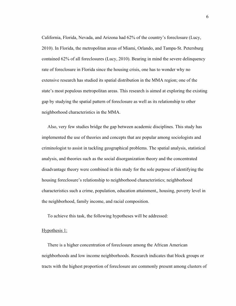
towns, and 9 villages (Figure 2). The county seat is located in the city of Miami, which is
also the largest of the incorporated city and the main economic hub of the county.
Figure 2. Study area showing the incorporated Communities in Miami-Dade County. The number ranking represents the location of each incorporated community (See Appendix B for table)
23

24
The city of Miami is the seat of Miami-Dade County, and it is located at the eastern
part of Miami-Dade metropolitan division along with the majority of the urbanized areas
in the county (Figure 2). It has a total land area 35.87 square miles with 11,135.9 persons
per square mile. The 2010 census on the city of Miami shows a total population of
399,457 people (US Census Bureau, 2013) out of which the major percentage of the
population goes to Whites and African American with 72.6% and 19.2% respectively.
The Hispanic or Latino ethnicity in the city of Miami makes up of about 70% of the total
population (US Census Bureau, 2013). Miami, been dubbed as “the capital city of Latin
America” comprises of a high percentage of Hispanic and Latino population. The city of
Miami and its suburbs are located on a broad plain between the Everglades to the west
and Biscayne Bay to the east. A total number of 117 census tract are located in the city of
Miami
3.3 Methodology
3.3.1 Data Sets
The data used for this study included the foreclosure counts, and 2010 Census data for
socioeconomic, population, racial composition, housing, and education attainment
variables for Miami-Dade County, and the city of Miami. Data collected specifically for
the city of Miami included the index crime data, and data on the vacant houses. All the
data used in this study were collected at the census tract level. The combinations of these
datasets were used on both Miami-Dade County, and the city of Miami to study
foreclosure relationships with the above mentioned variables.
25
1. Foreclosure data. Excel table format on a total of 18,155 foreclosure data containing
the addresses, market values, and date of foreclosure filing from 2010-2013 for the
housing units under foreclosure was purchased from a Miami-Dade foreclosure online
source (miamidadeforeclosures.com, 2013). Miamidadeforeclosure.com is the leading
online marketplace for foreclosure properties in Miami-Dade County. The data
comprised of information on the upcoming foreclosure, the cancelled foreclosure, and
those foreclosed houses that have been resold. It also showed the types of property, the
year the houses were built, and the bidding information for the auctioned sold houses.
2. Crime data. Crime data in excel table format from 2011-2012 was purchased from
the Miami-Dade Police Department showing the description of crimes committed, the
addresses, the time, and the dates of each reported crime incident. A total of 733, 994
crime cases were collected. The types of crime described in the data included
embezzlement, murder, forgery, false pretenses, driving under the influence of alcohol
(DUI), aggravated assault, receipt of stolen goods, rape, arson, burglary, etc. These data
which were purchased for the 117 census tract in the city of Miami was used to run
correlation and regression statistical analysis on the study area.
3. Socioeconomic and housing data. 2010 data was collected for the 519 census tracts
in Miami-Dade, and the 117 census tracts in city of Miami. A total number of 26
variables on various categories of the total population counts, socioeconomic, racial
composition, housing characteristics, and education attainment were collected from
American FactFinder (factfinder2.census.gov, 2013).

26
4. USPS vacant houses data. Embracing the social disorganization theory where
vacant and abandoned houses could be considered among the contributing factors which
leads to increase in crime, data on vacant houses was used in the foreclosure and crime
study. A compilation of the 2013 vacant houses data was collected from the U.S.
Department of Housing and Urban Development online portal (U.S. Department of
Housing and Urban Development, 2013). This data was collected at the census tract level,
and was used solely for studying the relationship between foreclosure, crime, and vacant
houses in the city of Miami. The data contained descriptions on a total of 316,075
housing addresses, out of which 13,577 were the total vacant addresses for the residential
and commercial properties in the city of Miami.
3.3.2 Software
Two types of software were used for this research. (1) ESRI ArcMap was used for
data processing and spatial analysis and (2) Statistical Package for the Social Sciences
(SPSS) was used for the statistical analysis.
3.3.3 Data Preparation
The foreclosure data downloaded were first classified under three foreclosure status
(1) upcoming, (2) cancelled, and (3) sold. The sold data category was used for studying
the spatial pattern of foreclosure in MMA. This is because only the sold houses listings
had data on the property’s appraisal, and contained the winning bid information for the
auctioned houses. The remaining two categories of foreclosed houses did not have their

27
market values attached to them, and this was an important criterion for identifying the
existence of a spatial pattern by using the housing market value. The first step in the data
preprocessing procedure required the conversion of the excel foreclosure and crime data
into geographic location on a map for spatial analysis. This is known as geocoding
(Figure 3, and Figure 4). A total number of 18,155 foreclosure addresses were
downloaded, 9,087 of which belonged to those foreclosed houses that have been sold to a
new homeowner or are considered a real estate owned property (REO). REO properties
are those foreclosed houses that are usually repossessed by a bank or a government loan
insurer after an unsuccessful sale at a foreclosure auction. This is common because most
of the bank-financed houses that make it to auction are worth less than the amount owed
to the bank. When this occurs the property becomes listed as a REO property and
categorized as an asset until the bank re-sells the property, usually through a real estate
agent. The sold houses listings might either be re-occupied or is a REO property waiting
to be sold or rented out.

28
Figure 3. Spatial representation of foreclosure distribution in Miami-Dade County
To address the issue of foreclosure and crime in the city of Miami, the second step is
selecting the index crime cases (both violent, and property crime indexes) according to
the Uniform Crime Report (UCR) classification. Florida, among the majority of the states
in the United States follows the guidelines set by the UCR handbook (U.S. Department of
Justice, 2004). The Federal Bureau of Investigation (FBI) set up the UCR program in the
1930s to collect a uniform crime statistics for the nation. Violent and property crimes
were the selected dataset used in this study. Other classification of crimes such as
embezzlement, forgery, false pretenses, driving under the influence of alcohol (DUI), and

29
receipt of stolen goods are not regarded as index crimes and are therefore not relevant for
this study. A total of 75,159 index crimes from 2011-2012 were downloaded and
geocoded; 6,727 were violent crimes while 68,432 were property crimes. Cui (2010)
weighed in in his study that foreclosure alone has no effect on crime, but the vacant
houses which serve as a disturb-free zone for criminal may be a contributing factor for
crime. In that spirit, the vacancy period of the REO properties were added into the study
of crime in the city of Miami to also examine how foreclosure and/or vacant houses
relates to crime. Attention should be drawn to the fact that the research on foreclosure,
vacancy and crime in this paper focuses on the city of Miami alone and not on Miami-
Dade County. The city of Miami was selected for the second phase because of it had the
highest population, highest foreclosure count, and highest crime total in the county; an
ideal location for the study.

30
Figure 4. Spatial representation of crime distribution in the city of Miami
The foreclosure process in Florida takes about 600 days to run its course from the first
notice until the date of sale. During this process lies the vacancy period where some
houses sold at auctions might not yet be re-occupied, or were classified as REO
properties and put back in the market (Figure 5). HUD has entered into an agreement
with the United States Postal Service (USPS) to receive quarterly aggregate data on
addresses identified by the USPS as having been "vacant" or "no-stat" in the previous
quarter. HUD makes these data available for researchers and practitioners to explore their
potential utility for tracking neighborhood change on a quarterly basis. The vacancy data
are produced only in census tract level, which was convenient since this study used
census tracts as a proxy for neighborhoods. HUD vacancy data collected for 2013 were

31
grouped into 4 quarterly data records. For this study, the data were aggregated from
January to December in order to get the median number of the total housing addresses,
and total vacant addresses. From the median vacant addresses, the residential vacant
buildings, commercial vacant buildings, and vacancy rate were acquired.
Foreclosure Process
Vacancy period
Figure 5. Foreclosure process
3.3.4 Spatial Analysis of Foreclosure and the Neighborhood Characteristics in MMA
The techniques applied in this study were for the purpose of identifying the spatial
pattern of foreclosure distribution across the MMA in Miami-Dade County. A similar
method was adopted by Seamon (2013) in Boston, and Schintler, Istrate, Pelletiere, and
Kulkarni (2010) in New England study area. The nearest neighbor analysis and spatial
autocorrelation were used to test for the presence of clustering of foreclosed houses in
MMA.
pre foreclosure Lis Pendens Sherriff Sale New Owner

32
1. Nearest neighbor analysis (NNA). NNA examines the distances between each point
on the map and the closest point to it from a complete random sample of point pattern
(Chen & Getis, 1998). This was carried out on the geocoded point data for sold
foreclosure houses to see the pattern of foreclosure in MMA. To determine the
distribution pattern, if the Nearest Neighbor index is less than 1, the pattern exhibits
clustering but if the index is greater than 1, the trend is toward dispersion. For the NNA,
the z- score and p-value results are measures of statistical significance, which tells
whether or not to reject the null hypothesis that features are randomly distributed. The p-
value is the probability that the observed spatial pattern was created by some random
process. When the p-value is very small (between -1.96 and +1.96,) it means it is very
unlikely that the observed spatial pattern is the result of random processes. This means
that the null hypothesis can be rejected. The z-score are simply standard deviations
associated with the normal distribution.
2. Spatial autocorrelation. Spatial autocorrelation identifies the pattern of the sold
foreclosure market value to determine if the data is thought to be clustered, dispersed or if
it occurs randomly. This was done to observe the possibility of an existing pattern among
areas of high and low market values of the foreclosed houses. Just like the NNA, the z-
score and p-value results are also measures of statistical significance, which tells whether
or not to reject the null hypothesis that features are randomly distributed. The p-value
result in the spatial autocorrelation is also the probability that the observed spatial pattern
was created by some random process. When the p-value is very small, it means it is very

33
unlikely that the observed spatial pattern is the result of random processes. This means
that the null hypothesis can be rejected.
3. Cluster and outlier analysis. The Moran's I test indicates spatial autocorrelation in
ArcMap. This was used to identify statistically significant hot spots, cold spots, and
spatial outliers using the Anselin Local Moran's I statistic. This tool identifies statistically
significant spatial clusters of high market values of foreclosed houses and low market
values of foreclosed houses. The purpose of this analysis is to identify the clustering
relationship and spatial distribution of foreclosure in MMA.
3.3.5 Statistical Analysis of Foreclosure and the Neighborhood Characteristics in MMA,
and Foreclosure and Crime in the City of Miami
1. Correlation analysis. Pearson’s correlation coefficient was first computed on a total
number of 26 variables. These variables acquired at the census tract level comprised of
the income, housing, population, racial composition, foreclosure, and education
attainment in Miami-Dade County, and the city of Miami. The purpose of correlating
these variables was to measure the strength of the association that existed among all the
26 variables.
2. Principal component analysis (PCA). PCA extracts a set of latent components that
explain as much of the covariance as possible from the aforementioned neighborhood
characteristics. PCA was carried out to identify groups of inter-correlated variables.
These variables accounted for the relationship between foreclosure, and the selected
components which were comprised of neighborhood characteristics in the study area.

34
3. Regression analysis. Several regression analyses depicting the relationship between
foreclosure and the neighborhood characteristics in MMA, and foreclosure and crime in
the City of Miami were used in the study. An exploratory analysis using the Enter Linear
Regression method on SPSS was carried out for the MMA. For the MMA, the foreclosure
rate was used as the dependent variables, and the components derived from the PCA that
accounts for most of the variance in the neighborhood characteristics as the independent
variables.
The second phase of the regression analysis was used to test H2 on the relationship
between foreclosure and crime. Based on recent literature on foreclosure and crime
(Immergluck & Smith, 2006; Cui, 2010), the following variables were constructed on
neighborhood characteristics that might be expected to affect crime:
Total population in Miami-Dade County for 2010
Percentage of all people below poverty level
Median family income in 2010
Vacancy rate
Foreclosure rate
Vacant residential addresses
Vacant business addresses
Percentage of income less than $10,000
Percentage of income $200,000 or more
Percentage of male population from 15 – 24
Percentage of Hispanic or Latino population
Percentage of Black or African American population

35
With crime as the dependent variable and the above indicators as the independent
variables, the relationship between crime (violent and property), vacancy, and foreclosure
were observed by using this equation.
Ci = a + b1Pi + b2Vi + b3Zi + b4Fi + Ei
Where:
Ci is the dependent variable representing the number of index crimes, with a
combination of both violent and property crime incidents in census tract i, and i will be
the unit of observation in a census tract. Pi is the population of the census tract, and Vi is
the vacant foreclosed houses in a census tract. Zi is a vector of characteristics that might
be expected to affect neighborhood crime; characteristics such as the male population
from 15-24 years, percentage of all people below poverty level, etc. Fi are census tract
level housing foreclosure rate. Foreclosure rate and vacancy rate were measured by
dividing each of them by the number of owner occupied housing units in the same census
tract (Immergluck, & Smith, 2006; Cui, 2010).

36
CHAPTER 4
RESULTS
4.1 Introduction
This chapter presents the foreclosure results from the MMA, and the foreclosure and
crime results from the city of Miami. An output of the visual representation acquired
from the spatial analysis and the result of the statistical analysis carried out in both study
areas was also portrayed in this chapter.
4.2 Nearest Neighbor Analysis Result for Foreclosure in MMA
The result shows a nearest neighbor index of 0.134. This result means there is
evidence of clustering among housing foreclosure. The z-score of -222.370 is outside the
critical value range between -1.96 and +1.96, indicating that there is a less than 1%
chance that the pattern is as a result of a random distribution. Thus, the pattern exhibited
is not the result of a random distribution but an unusual distribution; in this case,
clustering.
4.3 Spatial Autocorrelation Result for Foreclosure in MMA
The spatial autocorrelation result showed the clustering of similar market value
foreclosed houses to determine if a pattern exists among the clustered foreclosure houses
in MMA. The purpose of this result is to identify clustering patterns using the attribute
values as well as locations of the foreclosed houses. The z-score of 53.161 falls outside

37
the critical value range between -1.96 and +1.96. This shows that the pattern exhibited
among the foreclosed houses is the result of a clustered distribution.
4.4 Cluster and Outlier Analysis Results for Foreclosure in MMA
The z-score of the spatial autocorrelation analysis demonstrates the presence of
clustering in MMA. Spatial representation (Figure 6) displays the result of the Anselin
Local Moran's I statistic by showing areas of random distribution and those areas where
clustered values are surrounded by similar values. Clustering of foreclosed houses where
high market values are surrounded by similar high valued houses is represented with red
dots. The orange and light blue dots are those outliers where high market value houses
are surrounded with low market value houses and vice versa. The dark blue dots represent
the areas where houses of low market values are surrounded by similar values. Finally,
the black dots are areas where the distributions of houses market values are random.
Observations from the figure show a large amount of high market value clustering in the
city of Miami region in the central part of Miami-Dade County. The north and
southeastern parts show clustering of houses with low market values. The black dots
show a dense random distribution of foreclosed houses in the north-central section of
MMA.

38
Figure 6. Spatial distribution of foreclosure market value in MMA
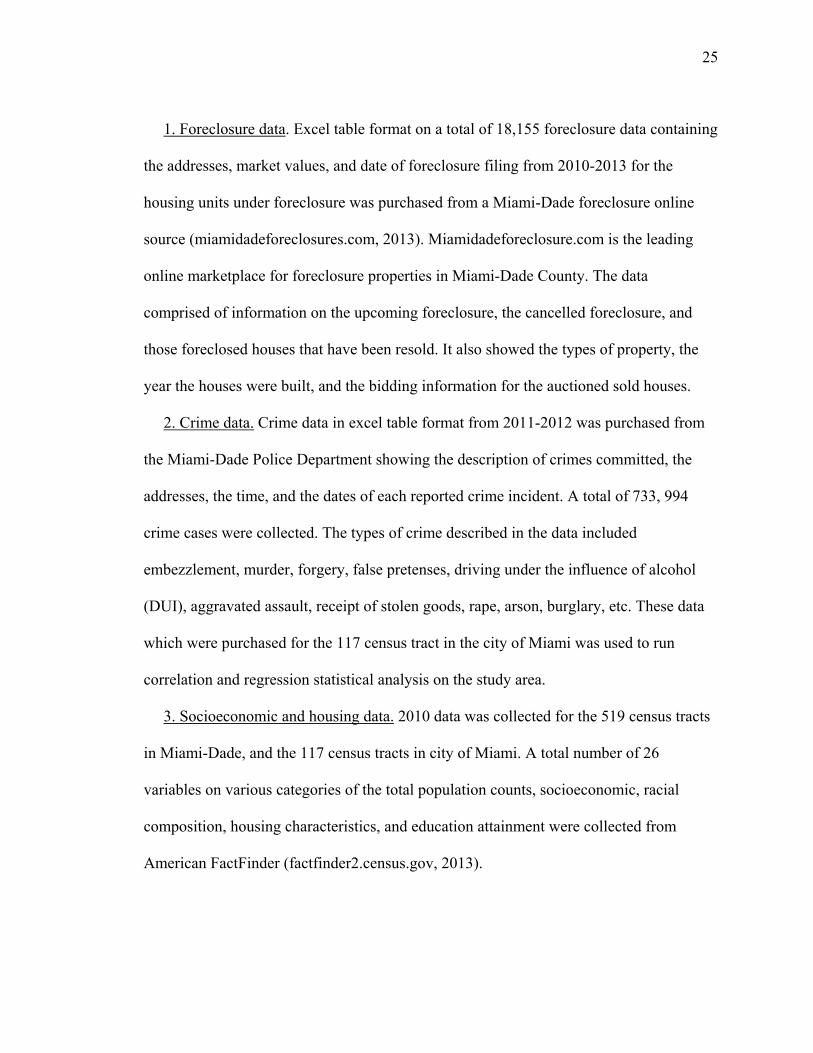
To test for H1 which is aimed at observing areas with increased foreclosure across the
major racial composition in MMA, Figure 7, Figure 8, and Figure 9 showed an overlay of
foreclosure counts over three racial groups. These three races which comprises of the
White, African American, and Asian population have been the focus of this study
because they make up 99.3% of the total population with 77.8%, 19.0%, and 1.7%

39
respectively (U.S. Census Bureau, 2013). The black dots in all three figures represent the
foreclosure count distribution across the county. In MMA, most of the foreclosed houses
are located on the eastern part of the county. This was expected considering the fact that
the western areas have lesser cities and populations in general. In the eastern part of the
county, the segregation pattern of the major racial compositions showed a high
foreclosure concentration among the African American population (Figure 8). In Figure
8, the visual representation of the map indicated that the cluster of foreclosed houses
especially at the northern part of the county was mostly occupied by the African
American population when compared to the rest of the other two races. With the
exception of the city of Miami, and Miami Beach region, the majority of the
neighborhood with a dominant White population in MMA showed a low concentration of
foreclosure (Figure 7). In Figure 9, the map indicated a low percentage of Asian
population in MMA, and among the Asian neighborhood, the presence of foreclosed
houses appeared to be low compared to that of the African American, and White
population. All three maps represented the foreclosure concentration among the dominant
racial groups in MMA.
40
Figure 7. Foreclosure count and the percent of White population in Miami-Dade County

41
Figure 8. Foreclosure count and the percent of African American population in Miami- Dade County

42
Figure 9. Foreclosure count and the percent of Asian population in Miami-Dade County

43
4.5 Correlation Analysis Results.
The Pearson correlation can take a range of values from +1 to -1. A value of 0
indicates that there is no association between the two variables. A value greater than 0
indicates a positive association, that is, as the value of one variable increases, so does the
value of the other variable. A value less than 0 indicates a negative association, that is, as
the value of one variable increases, the value of the other variable decreases. For this
study, there were 26 total number of variables selected to run the Pearson’s correlation
analysis. These 26 variables were comprised of the foreclosure rate, the total population
of people in MMA, the sex and age group of the population, median income and
education attainment for different education levels, housing data, employment status,
poverty level, population density, family household income, racial compositions, etc.
Among all the variables used for correlation, the foreclosure data, being the main focus of
this study showed the lowest correlation with other variables (Table 3). The highest
correlation with foreclosure rate from all 26 variables was with the population of people
in owner-occupied housing units (-.200). This means that an increase in foreclosure rate
indicates a decrease in the population of people in owner occupied housing unit.

44
Table 3. Foreclosure rate correlation with the selected 26 variables.
Variable Description Foreclosure rate
MEDFINC Median family income (dollars) -.066
MEDHINC Median household income (dollars) -.078
MEDINC25> Total median earnings in the past 12 months - population 25 years and over with earnings
.002
%BADEG> % - Bachelor's degree and higher -.059
%PINCPOV % of all people whose income in the past 12 months is below the poverty level
.119**
%FINCPOV Percentage of families whose income in the past 12 months is below the poverty level
.088
TOTMED Total median earnings - bachelor's degree and above .012
%INC200,000> % Income - $200,000 or more -.030
%INC<10,000 % Income - Less than $10,000 .069
POVRATE25> Total poverty rate for the population 25 years and over - bachelor's degree or higher
.049
LABFORCE Employment status - In labor force -.104*
TOTPOP Overall total population -.094*
TOTHH Income and benefits - Total households -.041
POHU Population in owner-occupied housing units -.200**
%TPH % of Total population in households .029
OHU Owner occupied housing units -.175**
FAMEMP Employment status - All parents in family in labor force -.040
%FAMEMP Employment status - Percent of All parents in family in labor force .002
UNEMP Employment status - In civilian labor force - Unemployed -.071
%HISP % Hispanic -.140**
%WHITE % White -.027
%AFA % African American .008
TOTHU Total housing units .093*
%ASIAN % Asian .015
%TP62> % of Total population - 62 years and over -.099*
POPDEN Population density .162**
**. Correlation is significant at the 0.01 level (2-tailed). *. Correlation is significant at the 0.05 level (2-tailed).

45
Table 4 shows the result of the correlation between socioeconomic variables and the
dominant racial and ethnic group in the study area. These racial and ethnic groups include
the White, African American, Asian, and the Hispanic population in MMA. There is a
positive correlation between Whites (%WHITE) and Asians (%ASIAN), and people who
attained a bachelor degree and higher (%BADEG>). %WHITE and %BADEG> showed
a high positive correlation result of .279, the same goes for %ASIAN and %BADEG>
with a positive correlation result of .262. This means that an increase in both the White
and the Asian population indicates an increase in people with a bachelor degree or higher.
The reverse was the case for the African American (%AFA) and Hispanic population’s
(%HISP) correlation with %BADEG>. %AFA and %HISP both showed negative
correlation results of -.273, and -.048 respectively. This means than an increase in both
the African American and the Hispanic population indicates a decrease in people with
bachelor degree or higher. The %AFA also showed high positive correlation (.416) with
people living below the poverty level (%PINCPOV). This means that the increase in the
African American population indicates an increase in people living below the poverty
level. Some of the highest coefficient results were between the variables containing the
dominant racial compositions like the %AFA, %WHITE, and %ASIAN, and the
%PINCPOV. The % WHITE and % ASIAN both point to a negative correlation of -.428,
and -.415 respectively with %PINCPOV. This means that an increase in either the White
or the Asian population indicates a decrease in people living below the poverty level.

46
Table 4. Correlation matrix between socioeconomic variables and ethnicity
4.6 Principal Component Analysis Result
Preliminary mandatory tests carried out as part of the PCA were the Kaiser-Meyer-
Olkin (KMO) and Bartlett’s test value (Liang & Weng, 2011). These two tests measure
the sampling adequacy of the variables used in PCA. PCA requires that the KMO
Measure of sampling adequacy be greater than 0.50 for the set of variables. Also an
acceptable data for PCA should have a significance level of the Bartlett’s test that is less
1 2 3 4 5 6 7 8 9 10
1 %BADEG> 1
2 POVRATE25> -.140
** 1
3 %WHITE .279 **
-.081 1
4 %HISP -.048 .066 .786 **
1
5 %AFA -.273
** .061
-.993 **
-.774 **
1
6 %ASIAN .262 **
-.251 **
.151 **
-.163 **
-.209 **
1
7 %INC<10,000 -.164
** .519 **
-.261 **
-.096 *
.259 **
-.351 **
1
8 %INC200,000> .422 **
-.239 **
.302 **
-.141 **
-.281 **
.282 **
-.265 **
1
9 MEDHINC .355 **
-.415 **
.343 **
-.042 -.326
** .421 **
-.565 **
.824 **
1
10 %PINCPOV -.300
** .542 **
-.428 **
-.182 **
.416 **
-.415 **
.782 **
-.381 **
-.661 **
1
**. Correlation is significant at the 0.01 level (2-tailed). *. Correlation is significant at the 0.05 level (2-tailed).

47
than .10 (Liang & Weng, 2011). The results of these two tests from the 26 variables used
showed a KMO value of .815 and a Bartlett’s test result of 0.000 which both implies the
suitability of the input variables for PCA. In order to further validate their capabilities, all
the 26 variables were checked for their communalities (Table 5). Communalities indicate
the amount of variance in each variable that is accounted for. Variables with small
communalities (less than 0.50) do not fit well with the PCA (Liang & Weng, 2011). Total
populations in household, all families in labor force, and population density failed to
meet the 0.50 cut off marker; these three variables were exempted from the subsequent
analysis. The remaining 23 variables left were used to run PCA.
The PCA result generated 6 components with the first 3 components together making
up to 71% of the total variance from all input variables (Table 6). Component 1
accounted for 34.2% of the total variance while components 2 and 3 accounted for 24.0%
and 12.7% respectively. These components were categorized as: Economic Indicator (EI)
for component 1, Crowdedness Indicator (CI) for component 2, and Racial Diversity
Indicator (RI) for component 3. The grouping of these variables into components was
done based on the high component scores of .70 and above amongst the variables used.
The variables that made up EI comprised of social and economic variables such as
MEDFINC, MEDHINC, MEDINC>25, %BADEG>, %PINCOV, % FINCOV,
%TOTMED, %INC200, 000>. The CI comprised of population and housing variables
with high component scores. These variables include LABFORCE, TOTPOP, TOTHH,
POHU, OHU, and FAMEMP. The variables that made up RI comprised of % HISP,

48
%WHITE and, %AFA. These three variables are the racial and ethnic composition in
MMA with a high component score.
Table 5. Communalities result from 26 variables
Communalities
Extraction POVRATE25> .545
TOTPOP .933 % WHITE .938 % HISP .899 % AFA .928 % ASIAN .589 %TPH .427 FAMEMP .708 %FAMEMP .470 %INC200,000> .767 %INC200,000> .847 MEDHINC .890 %FINCPOV .845
%PINCPOV .890
POPDEN .436 MEDINC25> .914
TOTMED .748 %TP62> .695 OHU .909 LABFORCE .931 UNEMP .706 TOTHH .937 %BADEG> .885 MEDFINC .904 TOTHU .866 POHU .925 Bold = <0.50

49
Table 6. PCA result showing 3 components
Component Matrix Component
1 2 3 MEDFINC .913 -.087 -.162
MEDHINC .912 -.007 -.186
MEDINC25> .887 -.156 -.183
%BADEG> .844 -.212 -.034
%PINCPOV -.835 -.146 -.042
%FINCPOV -.823 -.082 -.060
TOTMED .782 -.096 -.254
%INC200,000> .772 -.215 -.127
%INC<10,000 -.688 -.281 .083
POVRATE25> -.518 -.141 .295
LABFORCE .009 .956 .096
TOTPOP -.082 .955 .047
TOTHH -.070 .824 .210
POHU .334 .822 -.062
OHU .465 .796 -.004
FAMEMP -.073 .780 -.296
UNEMP -.411 .657 -.212
%HISP .093 .137 .883
%WHITE .533 -.034 .816
%AFA -.520 .038 -.807
TOTHU .085 .609 .126
%ASIAN .540 -.032 -.227
%TP62> .071 -.150 .546
Initial Eigenvalue 7.86 5.53 2.92% of Variance 34.21 24.05 12.73Cumulative % 34.21 58.26 70.99

50
4.6.1 Economic Indicator
The results for Figure 10 and Figure 11 show a comparison between the EI and the
White and African American population in the study area respectively. As earlier stated,
the majority of the populations in MMA are between the White, African American and
Asian populations. For this section a comparison between the Whites and African
American population with the EI was observed (these two races alone make up 96.8% of
the total population collectively; U.S. Census Bureau, 2013). Variables based on the PCA
analysis that had a higher score in the EI are MEDFINC, MEDHINC, MEDINC25>,
%BADEG>, %PINCPOV, %FINCPOV, TOTMED, and %INC200, 000>. All the listed
variables represent the economic condition of MMA (See Table 6). The darker portion of
the map portrays the areas with worse economic condition. The northern and southern
part of MMA show deficit in the EI while some areas at the middle of the metropolitan
division displays a much better EI condition in MMA. It can be observed from comparing
the result of the EI and the White population in Figure 10 that cities in MMA such as
Coral Gables, West Miami, South Miami, etc. that generally portrayed adequate
economic stimulus such as MEDINC25> and %BADEG> are located where a high
portion of the White population are found.

51
Figure 10. White population and EI locations in MMA
The segregation between the White, and the African American populations in Figure
10 and that of Figure 11 is noticeable. The African American population is more heavily
dominant at the municipalities in the northern part of the county such as Biscayne Park,
North Miami Beach, Miami Shores, North Miami etc.; the same areas with the lowest
values in EI. The isolated areas of the county identifying lower EI such as %PINCPOV
and %FINCPOV can be found in the northern and southern part of the study area. These
two results demonstrate an irrefutable difference of the economic situation in areas where
Whites and areas where African Americans are dominant.

52
Figure 11. African American population and EI locations in MMA
4.6.2 Crowdedness Indicator
The result for the CI as seen in Figure 12 is a random pattern of distribution across
Miami-Dade County. The area around the city of Miami appears to be showing the
lowest values in CI. This could be explained by the absence of land in most of the areas
in the tract due to the surrounding water bodies around the city of Miami, Miami Beach,
etc. This displays an incongruous result by portraying the presence of low CI in areas
where it does not exist.

53
Figure 12. CI showing random distribution in the study area
4.6.3 Racial Diversity Indicator
The variables based on the PCA analysis that have a higher score in the RI are
%HISP, %WHITE, and %AFA. All the listed variables represent dominant races and the
Hispanic ethnic population of MMA (See Table 6). The spatial representation for RI
(Figure 13) shows a high value of %AFA in the north and also a high value of %WHITE
and %HISP at the center where Hialeah and Miami municipal areas in Miami-Dade
County are located. The spatial representations showing the African American population
has been consistently placed in the same northern location throughout this study (See
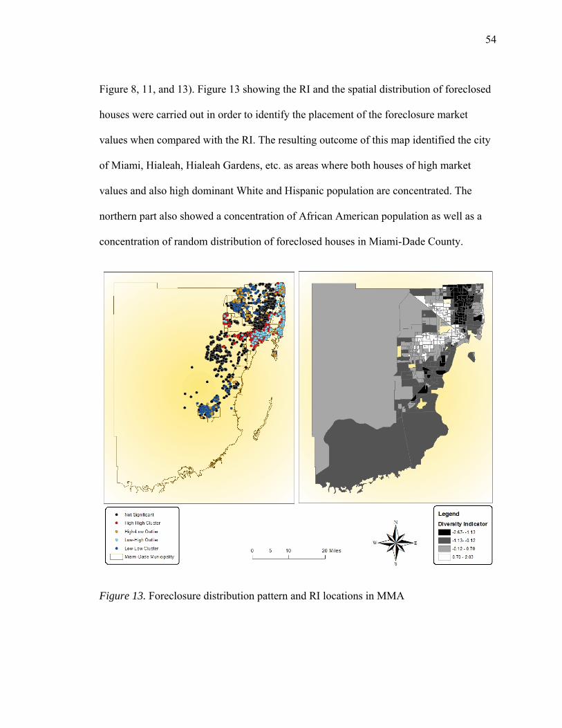
54
Figure 8, 11, and 13). Figure 13 showing the RI and the spatial distribution of foreclosed
houses were carried out in order to identify the placement of the foreclosure market
values when compared with the RI. The resulting outcome of this map identified the city
of Miami, Hialeah, Hialeah Gardens, etc. as areas where both houses of high market
values and also high dominant White and Hispanic population are concentrated. The
northern part also showed a concentration of African American population as well as a
concentration of random distribution of foreclosed houses in Miami-Dade County.
Figure 13. Foreclosure distribution pattern and RI locations in MMA

55
4.7 Results on the Regression Analysis for Foreclosure Rate in MMA
An exploratory regression analysis was carried out where foreclosure rate was used as
the dependent variable, and the three component results (EI, CI, and RI) of the PCA as
the independent variables. The independent variables contained a smaller number of
artificial variables that accounted for most of the variance from all 23 variables
representing the neighborhood characteristics in this study.
This model was used for the regression analysis:
Fi = a + b1EIi + b2CIi + b3RIi + Ei
Where Fi stands for foreclosure rate measured by the number of foreclosures divided by
the number of owner occupied housing unit in tract (Immergluck, & Smith, 2006; Cui,
2010). EI, represent Economic Indicator, CI represent Crowdedness Indicator and RI
represent Racial Diversity Indicator.
The foreclosure rate regression showed an insignificant result on two out of the three
independent variables. The regression model for foreclosure rate (r2 = .022,) showed how
much of the variability in the outcome is accounted for by the predictor. This means that
only 2.2% of the variance in foreclosure rate is explained. The result showed that for
every unit increase in CI there would be a .009 unit decrease in foreclosure rate. The
result on CI being the only significant output for the regression on foreclosure rate as the
dependent variable, has a significant level of .006; EI and RI had a significant level of
.179 and .224 respectively (Table 7). In an attempt to improve the regression output

56
shown for foreclosure rate, the squared version of the foreclosure rate index was
employed, but the unsquared version still yielded a better result. A less suitable result was
acquired from this approach where the r² = .009 which indicates that 0.9% of the variance
in the squared foreclosure rate is explained by all three independent variables. In the
second attempt, all three independent variables were insignificant contributors to
foreclosure in MMA. EI, CI, and RI all had a significant level of .982, .122, and .202
respectively (Table 7).
Table 7. Regression result on foreclosure rate and foreclosure rate squared
Foreclosure Rate Foreclosure Rate Squared
Coeff. Std. Error
Stdzd Coeff. Sig.
Coeff.
Std. Error
Stdzd Coeff. Sig.
(Constant)
.050
.003
.000
.007
.001
.000
EI
-.004
.003
.000
.179
-2.010E-05
.001
.001
.982
CI
-.009
.003
.179
.006
-.001
.001
-.072
.122
RI
-.004
.003
.006
.224
-.001
.001
-.059
.202
N
470
470
R²
.022
.009
Bold and underlined = Sig at P < 0.01; Bold = Sig at P ≥ 0.01 but p < 0.05; Underlined = Sig at P ≥ 0.05 but < 0.1

57
4.8 Sample Study on the Northern African American Population in MMA.
A second set of analyses was conducted on the northern part of MMA; the same area
with census tracts which contains 60 % and above of the African American population,
and also a high clustering of foreclosure (see Figure 8). The purpose of running a separate
analysis is to observe the possible result that could be acquired from using a sample
group in this study. By eliminating the outliers from the barren census tract in the western
part of MMA and focusing on a specific area with high foreclosure clustering, the
northern part of MMA was selected to study the relationship of foreclosure with the
selected variables in MMA. Out of the 519 census tract in MMA, 68 were selected for the
high risk sample study. The initial 26 selected variables were retained to run correlation
analysis, PCA, and regression analysis with the hope of achieving a more promising
result than that which was gotten from all 519 census tracts in MMA.
The overall correlation result between the foreclosure rate and the selected 26
variables improved greatly in the high risk sample group than when compared to that of
the initial analysis (Table 8). The highest correlation with foreclosure rate from all 26
variables was with the population of people in owner-occupied housing units (-.359).
This means that an increase in foreclosure rate indicates a decrease in the population of
people in owner occupied housing units. Other variables with high correlation includes
MEDFINC (-.287), MEDHINC (-.291), MEDINC25> (-.293), %BADEG> (-.262),
%PINCOV (.351), %FINCOV (.302), TOTMED (-.212), %INC<10,000 (.235),
LABFORCE (-.311), TOTPOP (-.288), OHU (-.355), UNEMP (-.229), %ASIAN (-.207),

58
and POPDEN (.302). Among the above 15 listed variables with high correlation with
foreclosure rate, 5 variables were significant at .01 level while 6 variables were
significant at .05 level. With the exception of %TP62>, the result acquired from the high
risk sample study’s 68 census tracts showed great improvement with the correlation and
the significant level than that of the initial 519 census tracts used.
From the high risk sample PCA, The results of the preliminary KMO, and Bartlett
tests for the 26 variables showed a value of .752 and 0.000 respectively which both
implies the suitability of the input variables for PCA. Unlike the initial PCA where 3 of
the variables were exempted for failure to meet the 0.5 communality marker, the PCA for
the high risk sample study showed that all 26 variables were above the 0.50 cut off
marker (Table 9). The PCA result generated 6 components with the first 3 components
together making up to 63% of the total variance from all input variables (Table 10); a
decrease from the initial PCA analysis which had 71% of the total variance for the first 3
components.

59
Table 8. MMA and AFA Foreclosure rate correlation with the selected 26 variables.
Variable Foreclosure rate of MMA
Foreclosure rate of AFA sample study
MEDFINC -.066 -.287*
MEDHINC -.078 -.291*
MEDINC25> .002 -.293*
%BADEG> -.059 -.262*
%PINCPOV .119** .351**
%FINCPOV .088 .302*
TOTMED .012 -.212
%INC200,000> -.030 -.096
%INC<10,000 .069 .235
POVRATE25> .049 .115
LABFORCE -.104* -.311**
TOTPOP -.094* -.288*
TOTHH -.041 -.166
POHU -.200** -.359**
%TPH .029 .183
OHU -.175** -.355**
FAMEMP -.040 -.191
%FAMEMP .002 -.105
UNEMP -.071 -.229
%HISP -.140** .004
%WHITE -.027 -.108
%AFA .008 .121
TOTHU .093* -.147
%ASIAN .015 -.207
%TP62> -.099* -.034
POPDEN .162** .302**
**. Correlation is significant at the 0.01 level (2-tailed). *. Correlation is significant at the 0.05
level (2-tailed).

60
From the high risk sample study, Component 1 accounted for 34.3% of the total
variance while components 2 and 3 accounted for 16.5% and 12.3% respectively.
Variables with high component scores (.70 and above) manifested more in the initial
PCA result than the high risk sample PCA result. Similar to that of the initial PCA result,
the components from the high risk sample were categorized as: Economic Indicator (EI)
for component 1, Crowdedness Indicator (CI) for component 2, and Racial Diversity
Indicator (RI) as component 3. These groupings are identical with that of the initial PCA
because of the similarity of the variables from both component results. RI remained
exactly the same in both results whereas changes were made to EI and CI. Variables such
as TOTMED, and %INC200, 000> that were present in the initial PCA were exempted
from the EI component of the high risk sample. Variables such as OHU, POHU,
%INC<10, 000, and LABFORCE that were exempted from the initial PCA were present
for the EI component of the high risk sample study. The remaining socioeconomic
variables such as %PINCOV, %FINCOV, TOTMED, %BADEG>, MEDINC25>,
MEDHINC, and MEDFINC were present in both EI component results. For the CI,
variables such as OHU, POHU, FAMEMP, and LABFORCE that were present in the
initial PCA were exempted from the CI component of the high risk sample. TOTHU
variable which was not included in the initial PCA was present among the CI component
of the high risk sample study. The remaining housing and population variables such as
TOTPOP and TOTHH were present in both CI component results. The 3 PCA component
results based on the high risk sample study were used as independent variables in Enter
Linear Regression analysis, where foreclosure rate was the dependent variable.

61
Table 9. Communalities result from MMA and AFA 26 variables
Communalities of MMA Communalities of AFA sample
study
Extraction Extraction
POVRATE25> .545 .649
TOTPOP .933 .968
% WHITE .938 .968
% HISP .899 .887
% AFA .928 .970
% ASIAN .589 .617
%TPH .427 .746
FAMEMP .708 .820
%FAMEMP .470 .706
%INC200,000> .767 .585
%INC<10,000 .847 .842
MEDHINC .890 .937
%FINCPOV .845 .881
%PINCPOV .890 .867
POPDEN .436 .545
MEDINC25> .914 .825
TOTMED .748 .644
%TP62> .695 .723
OHU .909 .869
LABFORCE .931 .906
UNEMP .706 .626
TOTHH .937 .891
%BADEG> .885 .730
MEDFINC .904 .921
TOTHU .866 .844
POHU .925 .838
Bold = <0.50

62
Table 10. PCA result from AFA sample study showing 3 components
Component Matrix
Component
1 2 3 OHU .897 .194 .058
POHU .889 .160 -.014
MEDHINC .857 -.440 .018
MEDFINC .852 -.430 .058
%PINCPOV -.831 .396 .075
%FINCPOV -.813 .444 .077
LABFORCE .803 .497 .100
%INC<10,000 -.759 .331 .187
MEDINC25> .756 -.396 .231
%BADEG> .735 -.224 .126
TOTMED .523 -.195 .051
%ASIAN .496 -.225 -.447
TOTHH .465 .786 .214
TOTHU .405 .777 .226 TOTPOP .668 .715 .089 UNEMP .397 .604 .245
POVRATE25> -.108 .513 -.229
%AFA -.287 -.194 .907
%WHITE .270 .191 -.906
%HISP .127 .263 -.881
%FAMEMP .237 -.092 .184
%TP62> .015 -.160 .070
FAMEMP .446 .486 .254
%TPH .095 -.100 .043
POPDEN -.309 -.138 .104
%INC200,000> .372 -.171 .333
Initial Eigenvalue 8.92 4.28 3.20 % of Variance 34.32 16.47 12.30 Cumulative % 34.32 50.79 63.09

63
The foreclosure rate regression showed an improvement from r2 = .022 in the initial
regression analysis to r2 = .168 in the high risk sample regression analysis. The CI was
the only notable significant output among the three variables results retrieved from the
initial regression analysis, whereas in the high risk sample study, only the EI had a
notable significant level of .001. The regression result for EI indicates that for every
increase in EI there would be a .017 unit decrease in foreclosure rate. CI and RI had a
significant level of .827 and .925 respectively (Table 11).
Table 11. Regression result on MMA and AFA sample study foreclosure rate
Foreclosure Rate on MMA
Foreclosure Rate on AFA sample study
Coeff. Std. Error
Stdzd Coeff. Sig.
Coeff.
Std. Error
Stdzd Coeff. Sig.
(Constant)
.050
.003
.000
.038 .005 .000
EI
-.004 .003 .000 .179 -.017 .005 -.409
.001
CI -.009 .003 .179
.006 -.001 .005 -.025
.827
RI -.004 .003 .006
.224 .000 .005 .011
.925
N 470 66
R² .022 .168 Bold and underlined = Sig at P < 0.01; Bold = Sig at P ≥ 0.01 but p < 0.05; Underlined = Sig at P ≥ 0.05 but < 0.1

64
4.9 Results on the Correlation and Regression Analysis for the City of Miami
The cluster and outlier analysis and the results from the PCA both point towards the
city of Miami as an area of interest with high value of the EI, and also a higher evidence
of clustering of high market value foreclosed houses than the rest of the county. This is
no surprise considering the city of Miami is a major hub in Miami-Dade County. To
further examine the city of Miami, an intricate study relating foreclosure and crime was
carried out.
Results from Pearson’s correlation shows that 9 of the neighborhood characteristics
have a positive correlation with violent crime: Percentage of African American
population (%AFA), percentage of people below poverty level (%PINCPOV), vacant
residential addresses (VACRES), and percentage of income less than $10,000
(%INC<10,000) have the highest positive correlation with violent crime which are
significant at the .01 level (r = .548, r = 512, r = 411 and r = 379 respectively)(Table 12).
For the property crime, vacancy rate (VACRATE), median vacant residential houses
(VACRES), percentage of people below poverty level (%PINCPOV), total vacant
addresses (TOTVAC), and percentage of income less than $10,000 (%INC<10,000) have
the highest positive correlation, which are significant at the .01 level (r = .469, r = .438, r
= .392, r = .258, and r = .250 respectively).

65
Table 12. Correlation result between crime and neighborhood characteristics
Correlations
Variable Description
Violent Crime
Property Crime
Total Crime
TOTPOP Overall total population
.138 .241** .235*
MEDFINC Median family income (dollars)
-.353** -.290** -.316**
%PINCPOV Percentage of all people whose income in the past 12 months is below the poverty level
.512** .392** .433**
MALE 15 - 24 Male 15 – 24
.250** .249** .261**
%WHITE % White
-.562** -.303** -.362**
%AFA % Black or African American
.548** .260** .321**
%HISP % Hispanic or Latino
-.334** -.172 -.208*
VACRES Median vacant residential addresses
.411** .438** .458**
VACBUS Median vacant business addresses -.088 -.026 -.038
TOTVAC total vacant addresses .193* .258** .262**
VACRATE vacancy rate .292** .469** .471**
%INC<10,000 Income - Less than $10,000 .379** .250** .286**
%INC200,000> Income - $200,000 or more -.317** -.289** -.309**
FORATE foreclosure rate
.163 .157 .163
**. Correlation is significant at 0.01 level (2-tailed). *. Correlation is significant at 0.05 level (2-tailed).
The results of the correlation analysis showed that most of the variables are significant
with both violent, and property crime, but the result of the correlations are, of course,
only indicative of the relationships that must be investigated by using a multiple
regression model. Correlation analysis tests the strength of the relationship between two

66
variables, regression analysis, on the other hand, make a stronger claim; they attempt to
demonstrate the degree to which one or more variables potentially promote positive or
negative change in another variable.
Examining the relationship between foreclosure-led vacant houses, and crime in the
city of Miami required the incorporation of the regression model discussed in the
methodology (Ci = a + b1Pi + b2Vi + b3Zi + b4Fi + Ei) to test for H2, and to explain the
effect of crime on foreclosure. Using the index crime in the city of Miami as the
dependent variables, both violent, and property crime were examined separately to run
the regression. Violent and property crime are both regarded as index crimes, but they
both require separate types of attention. A total of 75,159 index crimes were collected for
this study, 6,727 comprised of violent crimes, while 68,432 were property crimes.
Although the total number of violent crimes appears considerably lesser in comparison to
property crimes, violent crimes tends to attract more attention. In most cases, violent
crimes have a better chance of being reported when related to vacant and abandoned
buildings. Also, the effect of property crime may be greater in lower income
neighborhoods, but high income neighborhoods have a higher chance of reporting such
crimes that may be considered of less consequence in low income neighborhoods
(Immergluck, and Smith, 2006). To further examine crime, foreclosure, and vacant
houses, the Enter Linear Regression was conducted on violent crime, property crime, and
a combination of both (total crime) The independent variables consisted of the vacant
properties data (residential, and commercial), demographic characteristics, foreclosure
rate, and socioeconomic variables for all 117 census tracts in the city of Miami.

67
From the regression result, the model r2 for violent crime (r2 = .414) and property
crime (r2 = .449) shows a measure of how much of the variability in the outcome is
accounted for by the predictor (Table 13). This means that all of the independent
variables accounted for 41.4% of the variation in violent crime and 44.9% in property
crime. The regression result with total crime as the dependent variable is a combination
of both violent and property crime. In total crime, VACRATE, VACRES, %PINCPOV,
and %AFA have the highest positive correlation, which are significant at the .01 level (r
= .471, r = .458, r = .433, and r = .321 respectively). The model r2 (r2 = .462) for total
crime shows a measure of how much of the variability in the outcome is accounted for by
the predictor. This means that all of the independent variables accounted for 46.2% of the
variation in total crime.
Violent crime result shows an insignificant result on all counts with the exception of
the %AFA population leading to a 1.04 increase in crime with a significance level of
.062. The result could be argued as a non-contributive factor for influencing crime in the
real world.
In property crime, six of the demographic variables were statistically significant to
neighborhood crime. These include total population (TOTPOP), VACRATE, VACBUS,
percent of income above $200,000 (%INC200000>), %HISP and %AFA. All of the
above mentioned indicators were significant at the 0.01 level with the exception of
percent of income above $200,000 and percent of African American population. The
result showed that for every unit increase in VACRATE and TOTPOP, there would be a

68
45.686 and .087 unit increase in property crime respectively. Also, for every unit increase
in VACBUS, %INC200, 000>, and the %HISP, there would be a unit decrease of 1.734,
23.343, and 10.109 in property crime respectively.
From the total crime result in the regression analysis, TOTPOP, VACRATE, and
VACBUS are all significant at the .01 level. %INC200000> and %HISP are both
significant at P ≥ .01 but < 0.05. The result showed that for every unit increase in
TOTPOP, and VACRATE, there would be a .093 and 48.594 unit increase in total crime
respectively. Also, for every unit increase in VACBUS, %INC200000>, and %HISP,
there would be a unit decrease of 1.885, 24.010, and 9.911 in total crime respectively.

69
Table 13. Regression of crime on neighborhood characteristics and foreclosure rate in the city of Miami
Violent Crime Property Crime Total Crime
Coeff.Std.
Error Stdzd Coeff. Sig. Coeff.
Std. Error
Stdzd Coeff. Sig. Coeff.
Std. Error
Stdzd Coeff. Sig.
(Constant) -12.922 46.191 .780 905.165 293.078 .003 886.734 322.759 .007
% of all people below poverty level .808 .811 .163 .321
4.792 5.143 .148 .354
5.465 5.664 .151 .337
Median family income .000 .000 -.049 .719 .000 .002 -.022 .867 .000 .002 -.025 .849
Total population .005 .004 .140 .178 .087 .024 .359 .000 .093 .027 .343 .001
vacancy rate 1.675 1.842 .129 .365 45.686 11.688 .538 .000 48.594 12.872 .513 .000
foreclosure rate -25.713 119.644 -.018 .830 622.780 759.129 .066 .414 563.340 836.009 .054 .502
Vacant residential addresses .065 .154 .059 .675 -.381 .975 -.053 .697 -.349 1.073 -.044 .746Vacant business addresses -.101 .093 -.116 .279 -1.734 .589 -.305 .004 -1.885 .648 -.297 .004% Income Less than $10,000 -.129 1.043 -.017 .902 -6.341 6.620 -.130 .340 -6.275 7.291 -.115 .391
% Income $200,000 or more -.567 1.505 -.055 .707 -23.343 9.548 -.346 .016 -24.010 10.515 -.320 .024% Male 15 – 24 .178 1.040 .014 .864 -6.846 6.600 -.083 .302 -6.660 7.268 -.073 .362% Hispanic or Latino .123 .574 .048 .830 -10.109 3.640 -.599 .007 -9.911 4.009 -.527 .015% Black or African American 1.040 .552 .419 .062 -7.454 3.505 -.458 .036 -6.121 3.860 -.338 .116
N 117 117 117
R² 0.414 0.449 0.462
Bold and underlined = Sig at P < 0.01; Bold = Sig at P ≥ 0.01 but p < 0.05; Underlined = Sig at P ≥ 0.05 but < 0.1
69

70
CHAPTER 5
DISCUSSIONS
5.1 Introduction
This chapter discusses the findings of this study based on the results gotten from both
spatial, and statistical analysis in relation to foreclosure in MMA, and the city of Miami.
5.2 Foreclosure and Neighborhood Characteristics in MMA
The spatial analysis showed a concentration of foreclosure on the eastern part of
MMA. Most of the foreclosure listings were clustered on the municipalities surrounding
the city of Miami (see figure 6). The western part of the county had little or no cases of
foreclosure whatsoever. The northern part of MMA showed a high concentration of
random distribution of foreclosed houses. Areas where concentrations of high market
value foreclosed houses were surrounded by similar values consist of the city of Miami
and Miami Beach. The reason for the concentration of high market value foreclosed
houses in the city of Miami and the surrounding areas could be associated with the
geographic location. The geographic location of Miami and the beachside communities
north of Miami Beach: Surfside, Bal Harbour, Sunny Isles Beach, etc. attracts a higher
price of houses than other areas. These areas are considered among the top ten least
affordable housing options for moderate-income families in the nation’s 25 largest
metropolitan areas (Bandell, 2012; Kolko, 2014.)

71
The spatial analysis showed a pattern for foreclosure cases in MMA, the statistical
analysis on the other hand showed that foreclosure rate and most of the neighborhood
characteristics were not correlated at a significant level. The foreclosure rate showed a
negative correlation with the population of people in owner-occupied housing units (-
.200), and a positive correlation with percentage of people below poverty level (.119).
This means that an increase in foreclosure rate indicates a decrease in the population of
people in owner occupied housing unit, and an increase in foreclosure rate indicates an
increase in percentage of people below the poverty level. The negative correlation
between foreclosure rate and the population of people in owner-occupied housing units is
understandable. An increase in foreclosure is expected to reduce the number of people
still entitled to a house, especially in an area like the MMA where foreclosure cases are
well above average. Looking at the rest of the variables in the study to address H1,
disparities exist when relating the three observed racial compositions and the
socioeconomic variables. From the correlation analysis, the poverty rate of people 25
years and above, the percent of all people whose income is below the poverty level, and
the percentage of people whose income are less than $10,000 all have a positive
correlation with the African American population, and a negative correlation with the
White and Asian population. Whereas the percentage of people whose income are more
than $200,000, the median household income, and the percentage of people who attained
a bachelor degree and higher level of education all have a positive correlation with the
White and Asian population, but a negative correlation with the African American
population (see Table 4). This shows that in MMA, the socioeconomic status of the

72
African American population is less favorable compared to that of the Whites, or the
Asian population. This result on household income and race is somewhat similar to a
study conducted on the relationship between housing foreclosure, lending practice, and
neighborhood ecology (Kaplan & Sommers, 2009). Kaplan and Sommers (2009)
categorized the minority percentage in Summit County, Ohio as African American,
White Hispanic, and Asian American groups. In their correlation result between
foreclosure rate and the minority neighborhoods, the Hispanic and the Asian percentage
were small (1.1% and 1.8% respectively compared to the 14% for African American).
Their results showed that neighborhoods where subprime activity is exceptionally high
(over 22%) share a number of characteristics: they all have a high minority proportion
which primarily consists of the African American population. Generally, levels of income
are lower and poverty rates are higher. Like the studies referenced in H1 (Baxter &
Lauria, 1998; Chan et al., 2013; U.S. Department of Housing and Urban Development,
2000), the correlation analysis on individual variables in this study showed that among
the three racial compositions examined, the African American variable alone had
negative correlation with those socioeconomic variables that provides positive re-
enforcements which strengthens the social and economic status in their neighborhood.
This shows that the African American neighborhoods, being one of the dominant racial
groups in MMA, are a primary focus to be further observed in relation to the foreclosure
study.
The spatial output of the three components derived from the PCA analysis also points
that the African American population in the north showed deficiency in socioeconomic

73
stimulus. From the EI result, the northern part of MMA showed the lowest score whereas
the areas surrounding the city of Miami portrayed a much better economic standard. This
could explain why the city of Miami and its surrounding areas displayed a higher
concentration of high market valued foreclosed houses that the rest of the county. The
regression result generated from EI, CI, and, RI showed an unfavorable insignificant
relationship with foreclosure rate. The regression results with violent crime and property
crime as the dependent variables provided a much better model where r² = .414, and .449
respectively. Foreclosure rate and foreclosure rate squared which both used the PCA
component results as the independent variables, portrayed a model where r² = .022, and
.009 respectively. A possible explanation for the poor r² model could be because of the
combination of variables used. When consideration is given to the initial correlation
between the foreclosure rate and the same variables which made up those three
components, the poor regression results comes as no surprise.
The foreclosure rate variable from the high risk sample had a higher correlation with
the majority of the variables used. Variables with low correlation from the initial analysis
showed a much higher correlation when repeated with the fewer census tracts from the
high risk sample. There was an improvement in the high risk sample regression r² value
where r²= .168, yet the changes in the high risk sample result still did not improve the
regression between foreclosure rate and the 3 component score. The result still showed an
insignificant relationship with the selected independent variables. Unlike the correlation
analysis, the PCA from the high risk sample did not show much improvement. Although
the communalities result for the high risk sample showed that all the 26 variables were

74
accounted for, the cumulative percent of variance for the initial PCA was higher than that
of the high risk sample. Similar variables were identified in the RI results for the two
PCA analyses. EI and CI showed more variables in the initial PCA than that of the high
risk sample PCA. These changes did not account for much improvement from that of the
initial PCA, and they also did not assist in improving the relationship between foreclosure
rate and its independent variables as seen from the regression analysis result. Previous
studies conducted by Kaplan and Sommers (2009) in Summit County, Ohio, and
Mikelbank (2009) in Columbus, Ohio showed a more significant regression model for
foreclosure rate where r² = .47, and r² = .65 respectively. In this study, three regressions
were carried out using the un-squared MMA study area with 519 census tracts, the
squared MMA study area with 519 census tracts, and a high risk sample from the
northern part of MMA with 68 census tracts, but the result acquired from all three proved
insignificant to the relationship between foreclosure rate and the PCA scores. The
insignificant relationship in this study’s foreclosure cases could be as a result of the
deviation from the approach adopted by other studies, or it could simply mean that unlike
other study areas like Summit County, Ohio and Columbus, Ohio, foreclosure cases in
MMA have no significant relationship with its neighborhood characteristics. Perhaps a
possibility exists where the error lies with the variables used for this study.
Observing both the spatial and statistical analysis, the following can be said about the
northern part of Miami-Dade County. First, The EI is at its lowest in the north. Secondly,
there is a concentration of foreclosure cases at the northern part of Miami-Dade County,
and finally, the African American population appears to be heavily dominant in the north.

75
With the exception of the African American population, no other race or ethnic group
exhibited a high population in the northern part of Miami-Dade County. The spatial
representation of the African American population puts a large proportion of the
population in an area that shows a clustering of foreclosure and also a deficit in EI. Also,
the result from the correlation analysis shows African American populations as the only
race in Miami-Dade County to have a positive correlation with the percentage of people
living below poverty level and also a positive correlation with percentage income below
$10,000. All these contribute to the fact that amidst other races, the African American
population has a socioeconomic deficiency coupled with a higher case of foreclosure than
any other racial groups in MMA.
The correlation between %African American and foreclosure rates showed a weak
positive relationship, which at first seems surprising (Table 8). But foreclosure rate was
defined as the number of repossessed houses divided by owner occupied houses. If the
rates of home ownership are low for African Americans, the foreclosure rates could be
high but not affect the neighborhood. High rates of defaulting on mortgages may be part
of the story, but low rates of home ownership may override that relationship. Black inner-
city neighborhoods have been a prominent topic of discussion among social scientists and
criminologists (Shaw & McKay, 1942; Sampson & Wilson, 1995). These neighborhoods
have disproportionately suffered severe population and housing loss up to the point that it
begins to disrupt the social and institutional order (Sampson & Wilson, 1995). The theory
of concentrated disadvantage by Sampson and Wilson discusses on how the racial
differences in poverty and family disruption is so strong that the worst urban context in

76
which Whites resides are considerably better than the average context of Black
communities. Even when given the same objective socioeconomic status, Blacks and
Whites face vastly different environments in which to live, work, and raise their children
(Sampson & Wilson, 1995). The findings from this study fits in line with Sampson and
Wilson’s theory. It appears that the results strongly indicate that the African American
population are concentrated and residentially segregated in impoverished neighborhoods.
Several studies have proven that block groups or tracts with high proportions of
foreclosure are commonly present among clusters of African American populations and
low income neighborhoods (Chan et al., 2013; U.S. Department of Housing and Urban
Development, 2000). Spatial analysis in this study shows that in the case of MMA, both
tend to be located in the same area. A study on foreclosure conducted in Oakland showed
that foreclosure houses tend to be concentrated in minority neighborhoods with “higher-
than-typical crime rates and poor schools” (Williams, Weinheimer, & Brooks, 2011).
Oakland’s foreclosure problems was characterized by low income, high crime rates, poor
living conditions, etc. that were persuaded through predatory lending practices (Williams
et al., 2011). However, whether or not the concentration of foreclosure in the African
American neighborhood can be attributed to predatory lending through subprime
mortgage is beyond the scope of this study.
5.3 Foreclosure and Crime in the City of Miami
Both violent and property crime were statistically correlated with the majority of the
variables used in the study. Foreclosure rate and crime showed a weak relationship

77
compared to most of the variables (see Table 12). Foreclosure rate was significant at r =
.163, and .157 with violent and property crime respectively. The result between crime
and vacancy rate showed a better correlation than that of crime and foreclosure rate.
Crime and vacancy rate correlation showed r = .292 for violent crime, and r = .469 for
property crime, both which were significant at .01 level. The highest correlation with
violent crime were with %White, and %AFA. %White showed a negative correlation
with violent and property crime with r = -.562, and r = -303 respectively. The %AFA on
the other hand showed a positive correlation with r = .548 for violent crime, and r = .260
for property crime. The result from the correlation analysis indicates that increase in the
percentage of African American population leads to an increase in crime while the
percentage of White population has an inverse relationship with crime. The finding that
%AFA is one of the strongest correlates of crime is consistent with the theory of
concentrated disadvantage by Sampson and Wilson (1995). The concentrated
disadvantage theory, an updated version of Shaw and McKay’s social disorganization
theory, argues that a disproportionate amount of crime is associated with the
concentration of African Americans into communities, neighborhoods, housing projects,
etc. where poverty and unemployment rates are high, income levels are low, and divorce
rates and out of wedlock births are high. The regression analysis also explained a great
deal of the variance for all three crime index: violent crime with r2 = .414, property crime
with r2 = .449, and total crime with r2 = .462. From the regression result, violent crime in
general exhibited a statistically insignificant relationship with every variable in the study
except the African American variable. The analysis revealed a relationship between the

78
African American population and Crime, with a 1% increase in the Black or African
American population leading to 1% increase in violent crime. Yet the relationship among
the two variables had a significant level of .062 which does not incite confidence of the
outcome being a contributive factor in the real world. The result for violent crime in
previous studies showed a more significant relationship with variables such as the
number of businesses, unemployment rate, median family income, percentage low
education etc. (Immergluck & Smith, 2006; Katz et al., 2011). Property crime on the
other hand had a significant relationship with numerous variables such as the Hispanic
population, the African American population, the number of people whose income are
over $200, 000, and vacancy rate. With the exception of the vacancy rate, every other
significant demographic variable listed above indicated an inverse relationship with
property crime. Despite the strong positive correlation between crime and the African
American population, both variables representing the dominant minority group in the city
of Miami (Hispanic, and the African American) also indicated a negative relationship
with property crime. This indicates that the minority populations in the city of Miami are
not statistically significant determinants of property crime.
Investigating the relationship between foreclosure, vacancy, and crime in the city of
Miami was part of the primary objective of this study. The result from the regression
analysis shows that foreclosure rate, a primary variable for this analysis, indicated an
insignificant relationship with crime; both violent, and property. Immergluck and Smith’s
(2006) study on Chicago, Illinois revealed a direct relationship between foreclosure and
violent crime, whereas no relationship was observed between foreclosure and property

79
crime. Besides the insignificant relationship with foreclosure and crime in this study, no
relationship was observed between the variables on vacant houses and violent crime. In
property crime, vacancy rate was a statistical determinant with a 1% increase in vacancy
rate leading to a 45% increase in property crime. The rest of the variables representing
vacant houses in this study (vacant residential addresses, and vacant business addresses)
were statistically insignificant with property crime.
The result retrieved for the relationship between the vacant houses and crime were an
unexpected deviation from the expected outcome. Then again several factors needs to be
considered when attempting to relate different variables. It is possible that a better result
could still be achieved if a more consistent, standardized set of data was used throughout
the course of this study. The data used consisted of the total form (TOTPOP, TOTMED,
TOTHH, TOTHU), the percentage form (%AFA, %WHITE, %ASIAN, %TPH), and the
density form (POPDEN, FORATE, VACRATE) for the various variables. It is also
possible that a different result could be achieved if proper consideration were given to the
underlying size of the tracts in this study. The results may be biased simply because the
size of the tracts was not clued into the outcome of the analysis. The reason for pointing
all these out is to note that there are several factors at play which could be responsible for
the insignificant relationship between the foreclosure, crime, vacant data, and the vector
of neighborhood characteristics discussed in this study. Future studies could shed more
light on these points to explore the possibility of improving the results, especially after
the r2 result for the regression analysis in MMA proved to be poor on all fronts.

80
CHAPTER 6
CONCLUSIONS
6.1 Introduction
This chapter concludes the study by addressing the objectives and the hypotheses
introduced in Chapter 1, and the future direction which could be taken to further this
study. Also addressed are the limitations and the challenges encountered during the
course of this research, from data processing to analysis.
6.2 Conclusion
The purpose of this study was to (1) observe the clustering pattern of foreclosure in
MMA, (2) research the relationship between foreclosure and other neighborhood
characteristics at the census tract level and, (3) study the relationship between foreclosure
and crime in the city of Miami. For the purpose of this study, data of foreclosed houses in
Miami-Dade County was collected between 2010-2013 along with 2011-2012 crime data
and a census tract level database for the year 2010 containing information on
neighborhood characteristics. These were set up to achieve the following objectives:
1. Run nearest neighbor analysis, spatial autocorrelation, and cluster and outlier
analysis on the MMA to show its foreclosure distribution pattern.
2. Use correlation analysis, PCA, and regression analysis to check the relationships
between housing foreclosures and the 26 selected neighborhood attributes to
determine if any relationship exists in the MMA.

81
3. Run a regression analysis with the selected neighborhood attributes and also with
the vacancy period of the foreclosure process to study the relationship between
foreclosure, vacancy, and crime in the city of Miami, Florida.
Hypothesis 1 states that there is a higher concentration of foreclosure among the
African American neighborhoods and low income neighborhoods. In MMA, foreclosure
cases showed a clustering pattern. The city of Miami showed a concentration of high
market value foreclosure cases in MMA; an area predominantly occupied by the Whites
and Hispanic population. The entire northern part of MMA also showed a concentration
of foreclosure which appears to be the result of a random distribution. Unlike the city of
Miami which represents one of many areas with a high density population of White or
Hispanic population, the northern part of MMA represents a concentration of foreclosure
in neighborhoods predominantly occupied by the African Americans population. The
statistical analysis (correlation, PCA, and regression) showed that the foreclosure rate
observed in this study had no statistical significant relationship with the neighborhood
characteristics in MMA. Among other variables however, correlation, and PCA both
showed that the economic conditions in the White, and the Asian neighborhoods have
high positive correlation with variables depicting a better socioeconomic standing in
MMA. The African American neighborhood appeared to be significantly correlated with
characteristics showing that the area exhibits deficit in income and education attainment.
The visual representation of the different racial composition in MMA made it possible to
identify the segregation among the races, and to identify where each of the three racial
groups observed where dominant in number. This study accepts H1 which indicates an

82
increased presence of foreclosure in the African American neighborhood and low income
neighborhoods.
Hypothesis 2 states that the increase in foreclosure-led vacant houses leads to an
increase in crime. The result from the regression analysis showed that foreclosure was not
statistically significant with crime in the city of Miami, but the vacancy rate showed a
statistically significant relationship with property crime. Foreclosure rate and vacancy
rate showed no relationship whatsoever with violent crime. The vacant residential
addresses and the vacant business addresses both indicated a statistically insignificant
relationship with violent crime and property crime. This study rejects H2 which indicates
that an increase in foreclosure-led vacant houses leads to an increase in crime.
6.3 Limitations
While the researches carried out in this study were separated into categories, it is
crucial to state the shortcomings identified during the course of the whole thesis. Several
limitations were confronted, the greatest being the lack of accessible foreclosure data. A
total of 18,155 foreclosure data were downloaded for this study, but this was not the total
number of foreclosure filings in Miami-Dade County. Limitations placed on the number
of available downloads per day hindered the purchase of all of the foreclosure data. Also,
a time constraint and the inaccessibility of adequate and affordable foreclosure data for a
long period of time hindered the study of a temporal analysis showing the spatial
distribution of foreclosure.

83
Some foreclosure cases appeared for more than one foreclosure status. This means that
an address could show as an upcoming foreclosure and as a cancelled or sold foreclosure
at the same time. On a similar note, the foreclosure data descriptions were specific. It
recorded the date of foreclosure, the address, the foreclosure status, the type of property
that was foreclosed, etc. The vacancy data on the other hand showed less precise
information. There was no way to know the specific date a property became vacant, or if
all the vacant and abandoned properties were as a result of foreclosure. It is important to
note that not all foreclosed properties become vacant and abandoned, and not all vacant
and abandoned properties are the direct result of foreclosure. Despite the difficulty of
obtaining and processing of the foreclosure data, an accurate data on vacant and
abandoned buildings as a result of foreclosure proved to be more difficult to acquire. To
this end, the aggregate quarterly data at the census tract level of all the vacant houses in
the city of Miami was used.
6.4 Future Directions
This study leaves paths to be explored for further research and two are discussed here.
Justin Clark, an attorney who specializes in foreclosure cases believes that the foreclosure
recovery in Florida lags because unlike some other states, Florida's legal system prolongs
the foreclosure process. "Florida is a 'judicial state, meaning all foreclosures have to go
through the court." In addition, a Floridian's debt mounts quickly. “During a three-year
foreclosure process, a homeowner with a $1,500 monthly payment can quickly incur
$54,000 of late payments, plus legal fees and expenses. So while prices may be rising, the

84
amount owed increases even faster," Clark said (Shanklin, 2014). Considering the
different interest rates applied to mortgage holders, the expenses accrued from the home
loans that may inadvertently lead to foreclosure will be exponential for subprime loan
owners. A future study into foreclosure using data from home loans in MMA (both prime
and subprime loans) will examine the impact of subprime and predatory lending
mortgage and the possibility of an existing area or demography targeted for subprime
lending.
Besides the large scale effect of foreclosure on the economy, and the real estate
market in the United States, foreclosure also dealt a devastating blow on families, and
also brought distress to communities and municipalities. Addressing those communities
affected with foreclosure, little systematic researches have been conducted on
metropolitan responses to the foreclosure threat, and steps to be taken towards property
recovery. Property recovery is the new initiative adopted by many housing systems in
major metropolitan areas (Williams et al., 2011; Swanstrom, Chapple, & Immergluck,
2009). Both studies by Williams et al., (2011), and Swanstrom et al., (2009) were funded
by the MacArthur Foundation’s Building Resilient Regions (BBR) project to explore
regional solutions to foreclosure crisis. A similar method should be adopted in MMA to
assist in Federal and State policies towards mitigating foreclosure in the municipalities in
MMA.

85
REFERENCES
Amadeo, K. (2010). Homeowner stability Initiative to stop foreclosure. Retrieved from http://useconomy.about.com/od/candidatesandtheeconomy/a/foreclosure_bil.htm
Arnio, A. N., & Baumer, E. P. (2012, July 31). Demography, foreclosure, and crime:
Assessing spatial heterogeneity in contemporary models of neighborhood crime rates. Demographic Research, 26, 449-488.
Baker, D. (2008). The housing bubble and the financial crisis. Center for economic and
policy research, USA. Real-World Economic Review, issue no. 46. Bandell, B. (2012, October 18). Study: Miami-area housing least affordable for the
middle class. South Florida business journal. http://www.bizjournals.com/southflorida/blog/morning-edition/2012/10/study-miami-area-housing-affordable.html?page=all
Baxter, V. k., & Lauria, M. (1998, January 01). Housing foreclosure and racial transition
in New Orleans. Journal of Planning Literature, 15 (3). Baxter, V., & Lauria, M. (2001, January 01). Residential mortgage foreclosure and
neighborhood change. College of Urban and Public Affairs (CUPA) Working Papers, 1991 – 2000. Paper 18.
Blomquist, D. (2010). A record 2.8 million properties receive foreclosure notices in
2009. Retrieved from http://www.realtytrac.com/landing/2009-year-end-foreclosure-report.html
Brevoort, K. P., & Cooper, C. R. (2010). Foreclosure's wake: The credit experiences of
individuals following foreclosure. Washington, DC: Federal Reserve Board. Byun, K. J. (2010, December 01). The U.S. housing bubble and bust: Impacts on
employment. Monthly Labor Review, 133 (12), 3-17. Census tract data. (2010). Retrieved from http://factfinder2.census.gov/

86
Center for housing policy. (2014). September 2013 Metropolitan Delinquency and Foreclosure Data. Retrieved from http://www.foreclosure-response.org/maps_and_data/metro_delinquency_data_tables.html
Chan, S., Gedal, M., Been, V., & Haughwout, A. (2013, June 01). The role of
neighborhood characteristics in mortgage default risk: Evidence from New York City. Journal of Housing Economics, 22 (2), 100-118.
Chen, D., & Getis, A. (1998, May 12). Point Pattern Analysis. Retrieved from
http://ceadserv1.nku.edu/longa//geomed/ppa/doc/html/ppa.html Cui, L. (2010, November 1). Foreclosure, Vacancy and Crime. Available at SSRN:
http://ssrn.com/abstract=1773706 or http://dx.doi.org/10.2139/ssrn.1773706 Davies, J. (2014, April 11). Global financial crisis – What caused it and how the world
responded. Retrieved from http://www.canstar.com.au/home-loans/global-financial-crisis/
Delgadillo, L. & Erickson, L (2006). Spatial analysis of residential mortgage default in a
metropolitan County. Housing and Society, 33 (1), 39-47. Demyanyk, Y., & Hermert, O, V. (2009, May 04). Understanding the Subprime
Mortgage Crisis. Review of Financial Studies, 24 (6), 1848-1880. Ellen, I. G., Lacoe, J., & Sharygin, C. A. (2013, March 01). Do foreclosures cause crime?
Journal of Urban Economics, 74 (1), 59-70. Environmental Systems Research Institute (ESRI) (2014). Retrieved from
http://www.esri.com/what-is-gis FDIC, Office of the Inspector General. (2006). Challenges and FDIC Efforts Related to Predatory Lending. Audit report No. 06-011 Foreclosure data. (2010-2013). Retrieved from http://www.miamidadeforeclosures.com/

87
Goldstein, I., McCullough, M., Parker, A., & Urevick-Ackelsberg, D. (2005). A study by the reinvestment fund for the Pennsylvania Department of Banking. Mortgage foreclosure filings in Pennsylvania. Philadelphia Reinvestment Fund.
Herrmann, J, R. (2009). The American Nightmare: Exploring the Foreclosure Crisis in
Boston. Digital Collections and Archives, Tufts University. Immergluck, D., Alexander, F. S., Balthrop, K., Schaeffing, P., & Clark, J. (2011,
January 27). Legislative Responses to the Foreclosure Crisis in Non-judicial States. Available at SSRN: http://ssrn.com/abstract=1749609 or http://dx.doi.org/10.2139/ssrn.1749609
Immergluck, D., & Smith, G. (2005). There Goes the Neighborhood: The Effect of
Single-Family Mortgage Foreclosures on Property Values. Woodstock Institute, Chicago, IL. Retrieved from http://www.woodstockinst.org/sites/default/files/attachments/TGTN_Report%20%281%29_0.pdf
Immergluck, D., & Smith, G. (2006, November). The Impact of Single-family Mortgage
Foreclosures on Neighborhood Crime. Housing Studies, 21 (6), 851-866. Immergluck, D., Smith, G., & Woodstock Institute. (2004). Risky business: An
econometric analysis of the relationship between subprime lending and neighborhood foreclosures. Chicago, IL: Woodstock Institute.
Kaplan, D. H., & Sommers, G. G. (2009, February 01). An Analysis of the Relationship
between Housing Foreclosures, Lending Practices, and Neighborhood Ecology: Evidence from a Distressed County. The Professional Geographer, 61 (1).
Katz, C. M., Wallace, D., & Hedberg, E. C. (2011, December 26). A Longitudinal
Assessment of the Impact of Foreclosure on Neighborhood Crime. Journal of Research in Crime and Delinquency, 50 (3), 359-389.
Kolko, J. (2014, November 18). Where Is Homeownership Within Reach of the Middle
Class and Millennials? Retrieved from http://www.trulia.com/trends/2014/11/middle-class-millennials-report/

88
Laperriere, A. (2006, April 10) Housing bubble trouble: Have we been living beyond our means? The Weekly Standard Magazine, 11 (28).
Laperriere, A. (2007, March 12). House of Cards: The unsound loans that fueled the
housing boom are starting to collapse. The Weekly Standard Magazine, 12 (25). Liang, B., & Weng, Q. (2011, March 01). Assessing urban environmental quality change
of indianapolis, united states, by the remote sensing and GIS integration. IEEE Journal of Selected Topics in Applied Earth Observations and Remote Sensing, 4 (1), 43-55.
Lucy, W. H. (2010). Foreclosing the dream: How America's housing crisis is reshaping
our cities and suburbs. Chicago: American Planning Association, Planners Press. Mikelbank, B. A. (2009, January 1). Spatial Analysis of the Impact of Vacant,
Abandoned and Foreclosed Properties. Urban Publications. Paper 1024. Retrieved from http://engagedscholarship.csuohio.edu/urban_facpub/1024
Miller, J, M. (2009, September 17). 21st Century Criminology: A reference handbook.
Social Disorganization Theory. Article retrieved from http://www.sagepub.com/schram/study/materials/reference/90851_08.2r.pdf
Mummolo, J., & Brubaker, B. (2008, April 27). As foreclosure homes empty, crime
arrives. An article of the Washington Post retrieved from http://www.washingtonpost.com/wp-dyn/content/article/2008/04/26/AR2008042601288.html
Nembhard, J. G. (2010). Taking the Predator Out of Lending: The Role Played by
Community Development Credit Unions in Securing and Protecting Assets. Working Paper prepared for the Center on Race and Wealth, Howard University, Washington DC.
Office of Management and Budget. Executive office of the President. (2013, February
28). Revised Delineations of Metropolitan Statistical Areas, Micropolitan Statistical Areas, and Combined Statistical Areas, and guidance on uses of the delineations of these areas. OMB Bulletin No. 13-01

89
Olesiuk, S.M., & Kalser, R. K. (2009, April 27). The sand states: Anatomy of a perfect housing market storm. Federal Deposit Insurance Corporation. Article retrieved from https://www.fdic.gov/bank/analytical/quarterly/2009_vol3_1/AnatomyPerfectHousing.html
O’Toole, S. (2008, June 17). The Five D’s of Foreclosure. Article retrieved from
https://www.propertyradar.com/blog/five-ds-foreclosure/ RealtyTrac. (2007, February 8). More than 1.2 million foreclosure filings reported in
2006. Article retrieved from http://www.realtytrac.com/content/press-releases/more-than-12-million-foreclosure-filings-reported-in-2006-2234
RealtyTrac. (2008, January 30). U.S. foreclosure activity increases 75 percent in 2007.
Article retrieved from http://www.realtytrac.com/content/press-releases/us-foreclosure-activity-increases-75-percent-in-2007-3604
RealtyTrac. (2011, January 12). Record 2.9 million U.S. properties receive foreclosure
filings in 2010 despite 30-month low in December. Article retrieved from http://www.realtytrac.com/content/press-releases/record-29-million-us-properties-receive-foreclosure-filings-in-2010-despite-30-month-low-in-december-6309
RealtyTrac. (2013, January 14). 1.8 million U.S. properties with foreclosure filings in
2012. Retrieved from http://www.realtytrac.com/content/news-and-opinion/2012-year-end-foreclosure-market-report-7547
Sailer, S. (2009, April 23) Top 26 foreclosure rates all in 4 sand states. Retrieved from
http://www.vdare.com/posts/march-2009-top-26-foreclosure-rates-all-in-4-sand-states
Sampson, R, J., & Wilson, W, J. (1995). Toward a Theory of Race, Crime, and Urban
Inequality. In J. Hagan, & R.D. Peterson (Eds.), Crime and Inequality (pp. 37–54). Stanford, CA: Stanford University Press.

90
Schintler, L., Istrate, E., Pelletiere, D., & Kulkarni, R. (2010, October 15). The Spatial Aspects of the Foreclosure Crisis: A Look at the New England Region. GMU School of Public Policy Research Paper No. 2010-28. Available at SSRN: http://ssrn.com/abstract=1692969
Schloemer, E., Li, W., Ernst, K., & Keest, K. (2006). Losing Ground: Foreclosures in the
Subprime Market and Their Cost to Homeowners. Article retrieved from the Center for Responsible Lending. Available at http://www.responsiblelending.org/mortgage-lending/research-analysis/foreclosure-paper-report-2-17.pdf
Seamon, J. (2013, May 8). Home foreclosure risk in greater Boston: A search for
indicators. Urban Environmental Planning Policy, Tuft University. Available at http://sites.tufts.edu/gis/files/2013/11/Seamon_Jesse.pdf
Shanklin, M. (2014, October 23). Orlando, Polk, Brevard rank high in housing debt. Orlando Sentinel, FL. Available at http://www.orlandosentinel.com/business/os-underwater-houses-20141023-story.html
Shaw, C, R., & McKay, H, D. (1942). Juvenile delinquency and urban areas; a study of
rates of delinquents in relation to differential characteristics of local communities in American cities. Chicago, IL: University of Chicago Press.
Shaw, C, R., Zorbaugh, F, M., McKay, H, D., & Cottrell, L. S., National Institute on
Drug Abuse., & Addiction Research Center (U.S). (1929). Delinquency areas: A study of the geographic distribution of school truants, juvenile delinquents, and adult offenders in Chicago. Chicago, IL: University of Chicago Press.
Swanstrom, T., Chapple, K., Immergluck, D., University of California, Berkeley, &
MacArthur Foundation Research Network on Building Resilient Regions. (2009). Regional resilience in the face of foreclosures: Evidence from six metropolitan areas. Berkeley, CA: University of California, Institute of Urban and Regional Development.
United States Census Bureau. (2013). Retrieved from http://www.census.gov/

91
United States Department of Housing and Urban Development. (2000). Unequal burden: Income and racial disparities in subprime lending in America. Washington, DC.
United States Department of Housing and Urban Development. (2013). Vacancy data
Retrieved from http://www.huduser.org/portal/datasets/usps.html United States Department of Justice. Federal Bureau of Investigation. (2004). Uniform
crime reporting handbook: UCR. Washington, D.C. United States Department of Labor. (2014, April 23). Bureau of Labor Statistics. County
Employment and Wages In Florida – Third Quarter 2013. Atlanta, GA. United States Department of Labor. (2014. July 31). Bureau of Labor Statistics. Miami
Area Employment – June 2014. Atlanta, GA. United States Department of the Treasury. Troubled Asset Relief Program (U.S). (2011).
Troubled Asset Relief Program: Three year anniversary report: a supplement to the TARP two year retrospective. Washington, DC: U.S. Office of Financial Stability.
Wallison, P. J. (2009). The true origin of the financial crisis: As opposed to a desperate
liberal legend. Retrieved February, 2009 from http://spectator.org/articles/42211/true-origins-financial-crisis
Williams, R. L., Weinheimer, M., & Brooks, J. A. (2011, October). Resilience in the face of foreclosure: Six case studies on neighborhood stabilization. Center for research and innovation. National league of cities, Washington, DC.
Wilson, J. Q., & Kelling, G. L. (1982). Broken Windows: The police and neighborhood
safety. Article retrieved from http://www.manhattan-institute.org/pdf/_atlantic_monthly-broken_windows.pdf
Wilson, R. E., & Paulsen, D. J. (2008, October 01). Foreclosures and Crime: A
Geographical Perspective. Geography & Public Safety, 1 (3).

92
Wolff, K. T., Cochran, J. C., & Baumer, E. P. (2014, March 25). Reevaluating Foreclosure Effects on Crime during the "Great Recession." Journal of Contemporary Criminal Justice, 30 (1), 41-69.
Wong, C. (2011). The Social Disorganization Theory. Center for Spatially Integrated
Social Sciences by Regents of University of California, Santa Barbara. Article retrieved from http://www.csiss.org/classics/content/66
Xu, Y. & Zhang, J. (2012). Interstate non-local mortgage Lending: Features and
explanations. Retrieved from http://citeseerx.ist.psu.edu/viewdoc/download;jsessionid=66B6CD9C51D0E19E3BB6F47F81C29F49?doi=10.1.1.365.8903&rep=rep1&type=pdf
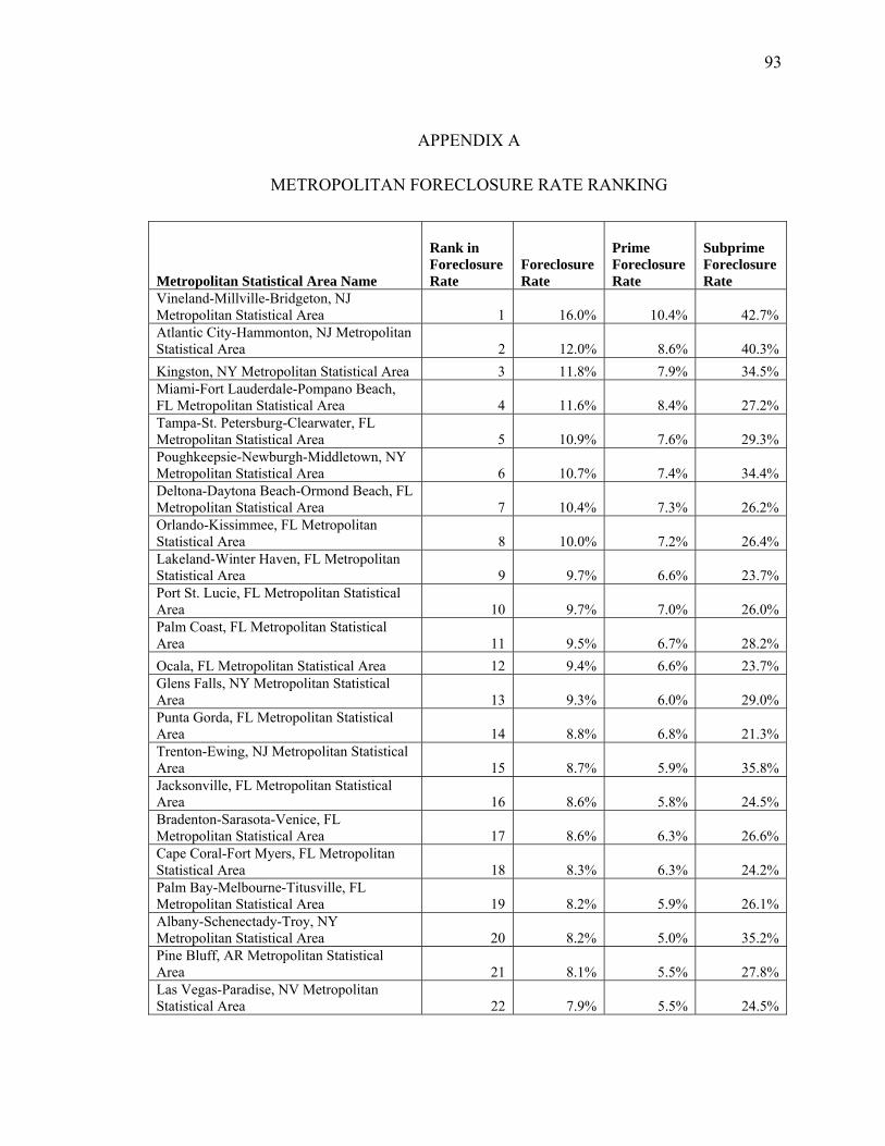
93
APPENDIX A
METROPOLITAN FORECLOSURE RATE RANKING
Metropolitan Statistical Area Name
Rank in Foreclosure Rate
Foreclosure Rate
Prime Foreclosure Rate
Subprime Foreclosure Rate
Vineland-Millville-Bridgeton, NJ Metropolitan Statistical Area 1 16.0% 10.4% 42.7% Atlantic City-Hammonton, NJ Metropolitan Statistical Area 2 12.0% 8.6% 40.3%
Kingston, NY Metropolitan Statistical Area 3 11.8% 7.9% 34.5% Miami-Fort Lauderdale-Pompano Beach, FL Metropolitan Statistical Area 4 11.6% 8.4% 27.2% Tampa-St. Petersburg-Clearwater, FL Metropolitan Statistical Area 5 10.9% 7.6% 29.3% Poughkeepsie-Newburgh-Middletown, NY Metropolitan Statistical Area 6 10.7% 7.4% 34.4% Deltona-Daytona Beach-Ormond Beach, FL Metropolitan Statistical Area 7 10.4% 7.3% 26.2% Orlando-Kissimmee, FL Metropolitan Statistical Area 8 10.0% 7.2% 26.4% Lakeland-Winter Haven, FL Metropolitan Statistical Area 9 9.7% 6.6% 23.7% Port St. Lucie, FL Metropolitan Statistical Area 10 9.7% 7.0% 26.0% Palm Coast, FL Metropolitan Statistical Area 11 9.5% 6.7% 28.2%
Ocala, FL Metropolitan Statistical Area 12 9.4% 6.6% 23.7% Glens Falls, NY Metropolitan Statistical Area 13 9.3% 6.0% 29.0% Punta Gorda, FL Metropolitan Statistical Area 14 8.8% 6.8% 21.3% Trenton-Ewing, NJ Metropolitan Statistical Area 15 8.7% 5.9% 35.8% Jacksonville, FL Metropolitan Statistical Area 16 8.6% 5.8% 24.5% Bradenton-Sarasota-Venice, FL Metropolitan Statistical Area 17 8.6% 6.3% 26.6% Cape Coral-Fort Myers, FL Metropolitan Statistical Area 18 8.3% 6.3% 24.2% Palm Bay-Melbourne-Titusville, FL Metropolitan Statistical Area 19 8.2% 5.9% 26.1% Albany-Schenectady-Troy, NY Metropolitan Statistical Area 20 8.2% 5.0% 35.2% Pine Bluff, AR Metropolitan Statistical Area 21 8.1% 5.5% 27.8% Las Vegas-Paradise, NV Metropolitan Statistical Area 22 7.9% 5.5% 24.5%
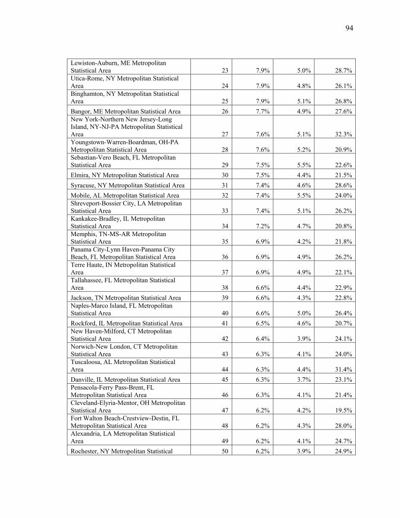
94
Lewiston-Auburn, ME Metropolitan Statistical Area 23 7.9% 5.0% 28.7% Utica-Rome, NY Metropolitan Statistical Area 24 7.9% 4.8% 26.1% Binghamton, NY Metropolitan Statistical Area 25 7.9% 5.1% 26.8%
Bangor, ME Metropolitan Statistical Area 26 7.7% 4.9% 27.6% New York-Northern New Jersey-Long Island, NY-NJ-PA Metropolitan Statistical Area 27 7.6% 5.1% 32.3% Youngstown-Warren-Boardman, OH-PA Metropolitan Statistical Area 28 7.6% 5.2% 20.9% Sebastian-Vero Beach, FL Metropolitan Statistical Area 29 7.5% 5.5% 22.6%
Elmira, NY Metropolitan Statistical Area 30 7.5% 4.4% 21.5%
Syracuse, NY Metropolitan Statistical Area 31 7.4% 4.6% 28.6%
Mobile, AL Metropolitan Statistical Area 32 7.4% 5.5% 24.0% Shreveport-Bossier City, LA Metropolitan Statistical Area 33 7.4% 5.1% 26.2% Kankakee-Bradley, IL Metropolitan Statistical Area 34 7.2% 4.7% 20.8% Memphis, TN-MS-AR Metropolitan Statistical Area 35 6.9% 4.2% 21.8% Panama City-Lynn Haven-Panama City Beach, FL Metropolitan Statistical Area 36 6.9% 4.9% 26.2% Terre Haute, IN Metropolitan Statistical Area 37 6.9% 4.9% 22.1% Tallahassee, FL Metropolitan Statistical Area 38 6.6% 4.4% 22.9%
Jackson, TN Metropolitan Statistical Area 39 6.6% 4.3% 22.8% Naples-Marco Island, FL Metropolitan Statistical Area 40 6.6% 5.0% 26.4%
Rockford, IL Metropolitan Statistical Area 41 6.5% 4.6% 20.7% New Haven-Milford, CT Metropolitan Statistical Area 42 6.4% 3.9% 24.1% Norwich-New London, CT Metropolitan Statistical Area 43 6.3% 4.1% 24.0% Tuscaloosa, AL Metropolitan Statistical Area 44 6.3% 4.4% 31.4%
Danville, IL Metropolitan Statistical Area 45 6.3% 3.7% 23.1% Pensacola-Ferry Pass-Brent, FL Metropolitan Statistical Area 46 6.3% 4.1% 21.4% Cleveland-Elyria-Mentor, OH Metropolitan Statistical Area 47 6.2% 4.2% 19.5% Fort Walton Beach-Crestview-Destin, FL Metropolitan Statistical Area 48 6.2% 4.3% 28.0% Alexandria, LA Metropolitan Statistical Area 49 6.2% 4.1% 24.7%
Rochester, NY Metropolitan Statistical 50 6.2% 3.9% 24.9%

95
Area
Kokomo, IN Metropolitan Statistical Area 51 6.1% 4.0% 21.1%
Monroe, LA Metropolitan Statistical Area 52 6.1% 4.7% 23.0% Chicago-Naperville-Joliet, IL-IN-WI Metropolitan Statistical Area 53 6.0% 4.3% 23.7% Montgomery, AL Metropolitan Statistical Area 54 6.0% 4.3% 24.7%
Akron, OH Metropolitan Statistical Area 55 6.0% 4.3% 20.1%
Anderson, IN Metropolitan Statistical Area 56 5.8% 4.1% 17.9% Scranton--Wilkes-Barre, PA Metropolitan Statistical Area 57 5.8% 3.8% 18.8% Buffalo-Niagara Falls, NY Metropolitan Statistical Area 58 5.8% 3.8% 24.5%
Dover, DE Metropolitan Statistical Area 59 5.8% 3.8% 25.1% Philadelphia-Camden-Wilmington, PA-NJ-DE-MD Metropolitan Statistical Area 60 5.7% 3.7% 23.7% Gainesville, FL Metropolitan Statistical Area 61 5.7% 3.8% 20.7% Allentown-Bethlehem-Easton, PA-NJ Metropolitan Statistical Area 62 5.6% 4.0% 23.2%
Topeka, KS Metropolitan Statistical Area 63 5.5% 3.8% 22.9%
Cleveland, TN Metropolitan Statistical Area 64 5.5% 3.9% 22.0%
Salem, OR Metropolitan Statistical Area 65 5.5% 3.8% 22.7%
Salisbury, MD Metropolitan Statistical Area 66 5.4% 3.6% 18.6%
Medford, OR Metropolitan Statistical Area 67 5.4% 4.1% 22.9% Ocean City, NJ Metropolitan Statistical Area 68 5.4% 3.7% 36.4% Mansfield, OH Metropolitan Statistical Area 69 5.4% 3.5% 17.6%
Ithaca, NY Metropolitan Statistical Area 70 5.3% 4.0% 19.1% Reno-Sparks, NV Metropolitan Statistical Area 71 5.3% 3.9% 21.5%
Jackson, MS Metropolitan Statistical Area 72 5.3% 3.1% 18.1%
Albany, GA Metropolitan Statistical Area 73 5.2% 3.6% 16.1% Rocky Mount, NC Metropolitan Statistical Area 74 5.2% 3.4% 16.2% Chattanooga, TN-GA Metropolitan Statistical Area 75 5.1% 3.2% 20.8%
Peoria, IL Metropolitan Statistical Area 76 5.1% 3.3% 22.4%
Pittsfield, MA Metropolitan Statistical Area 77 5.1% 2.9% 18.5% Springfield, MA Metropolitan Statistical Area 78 5.1% 2.8% 17.6% Hinesville-Fort Stewart, GA Metropolitan Statistical Area 79 5.1% 4.0% 19.4%
Flint, MI Metropolitan Statistical Area 80 5.1% 3.6% 13.8%
Erie, PA Metropolitan Statistical Area 81 5.1% 3.1% 19.2%

96
Dayton, OH Metropolitan Statistical Area 82 5.0% 3.6% 19.7% Baltimore-Towson, MD Metropolitan Statistical Area 83 5.0% 3.2% 22.3% Cumberland, MD-WV Metropolitan Statistical Area 84 5.0% 3.2% 17.9% Columbus, OH Metropolitan Statistical Area 85 5.0% 3.4% 21.7% Johnstown, PA Metropolitan Statistical Area 86 5.0% 3.0% 22.4% Portland-South Portland-Biddeford, ME Metropolitan Statistical Area 87 5.0% 3.4% 24.8%
Dothan, AL Metropolitan Statistical Area 88 5.0% 3.9% 22.6% Bridgeport-Stamford-Norwalk, CT Metropolitan Statistical Area 89 5.0% 3.3% 22.3% Indianapolis-Carmel, IN Metropolitan Statistical Area 90 4.9% 3.3% 20.8% Cincinnati-Middletown, OH-KY-IN Metropolitan Statistical Area 91 4.9% 3.6% 20.0% Michigan City-La Porte, IN Metropolitan Statistical Area 92 4.9% 3.2% 17.6% Wichita Falls, TX Metropolitan Statistical Area 93 4.9% 3.8% 19.5% Springfield, OH Metropolitan Statistical Area 94 4.9% 3.4% 16.6% Providence-New Bedford-Fall River, RI-MA Metropolitan Statistical Area 95 4.9% 3.3% 18.1%
Sandusky, OH Metropolitan Statistical Area 96 4.9% 3.4% 18.1%
Macon, GA Metropolitan Statistical Area 97 4.8% 3.3% 14.5% Little Rock-North Little Rock-Conway, AR Metropolitan Statistical Area 98 4.8% 3.3% 25.1%
Muncie, IN Metropolitan Statistical Area 99 4.8% 3.3% 15.1% Worcester, MA Metropolitan Statistical Area 100 4.8% 2.9% 20.5%
Lima, OH Metropolitan Statistical Area 101 4.8% 3.0% 12.6%
Honolulu, HI Metropolitan Statistical Area 102 4.8% 3.1% 26.0%
Lawton, OK Metropolitan Statistical Area 103 4.8% 3.3% 20.6% New Orleans-Metairie-Kenner, LA Metropolitan Statistical Area 104 4.7% 3.0% 19.3%
Bend, OR Metropolitan Statistical Area 105 4.7% 3.5% 26.1%
Janesville, WI Metropolitan Statistical Area 106 4.7% 3.2% 17.7%
Reading, PA Metropolitan Statistical Area 107 4.7% 3.3% 20.9%
Dalton, GA Metropolitan Statistical Area 108 4.6% 3.3% 17.2% South Bend-Mishawaka, IN-MI Metropolitan Statistical Area 109 4.6% 2.9% 14.8% Weirton-Steubenville, WV-OH Metropolitan Statistical Area 110 4.6% 3.3% 11.9%
Decatur, IL Metropolitan Statistical Area 111 4.5% 2.7% 18.5%

97
York-Hanover, PA Metropolitan Statistical Area 112 4.5% 3.1% 22.0%
Sumter, SC Metropolitan Statistical Area 113 4.5% 2.9% 16.0% Goldsboro, NC Metropolitan Statistical Area 114 4.4% 3.1% 18.0% Fort Smith, AR-OK Metropolitan Statistical Area 115 4.4% 3.0% 18.6% Milwaukee-Waukesha-West Allis, WI Metropolitan Statistical Area 116 4.4% 2.9% 21.6%
Racine, WI Metropolitan Statistical Area 117 4.4% 3.1% 18.7% Evansville, IN-KY Metropolitan Statistical Area 118 4.4% 3.0% 19.9%
Columbia, SC Metropolitan Statistical Area 119 4.4% 2.9% 18.1% Brunswick, GA Metropolitan Statistical Area 120 4.3% 3.4% 15.6% Columbus, GA-AL Metropolitan Statistical Area 121 4.3% 3.0% 18.1% Augusta-Richmond County, GA-SC Metropolitan Statistical Area 122 4.3% 3.0% 19.5%
Rome, GA Metropolitan Statistical Area 123 4.3% 3.4% 16.2% Elkhart-Goshen, IN Metropolitan Statistical Area 124 4.3% 2.8% 16.6% Hartford-West Hartford-East Hartford, CT Metropolitan Statistical Area 125 4.3% 2.6% 20.5% LouisvilleJefferson County, KY-IN Metropolitan Statistical Area 126 4.3% 2.9% 20.6% Saginaw-Saginaw Township North, MI Metropolitan Statistical Area 127 4.2% 3.1% 11.9% Anniston-Oxford, AL Metropolitan Statistical Area 128 4.2% 2.9% 19.6% Elizabethtown, KY Metropolitan Statistical Area 129 4.2% 3.0% 19.3% Fort Wayne, IN Metropolitan Statistical Area 130 4.2% 2.9% 17.8%
Savannah, GA Metropolitan Statistical Area 131 4.2% 3.0% 16.6% Pascagoula, MS Metropolitan Statistical Area 132 4.1% 2.7% 15.6% Hagerstown-Martinsburg, MD-WV Metropolitan Statistical Area 133 4.1% 3.0% 17.5% Eugene-Springfield, OR Metropolitan Statistical Area 134 4.1% 2.8% 21.4% Birmingham-Hoover, AL Metropolitan Statistical Area 135 4.1% 2.7% 18.3%
Yakima, WA Metropolitan Statistical Area 136 4.1% 2.7% 16.3% Canton-Massillon, OH Metropolitan Statistical Area 137 4.1% 3.0% 13.2%
Valdosta, GA Metropolitan Statistical Area 138 4.1% 2.8% 23.0% Lake Charles, LA Metropolitan Statistical Area 139 4.1% 2.8% 20.0%

98
Toledo, OH Metropolitan Statistical Area 140 4.0% 2.9% 15.1% Hot Springs, AR Metropolitan Statistical Area 141 4.0% 3.1% 22.4% Longview, WA Metropolitan Statistical Area 142 4.0% 2.8% 18.6% Carson City, NV Metropolitan Statistical Area 143 4.0% 3.1% 14.6%
Pittsburgh, PA Metropolitan Statistical Area 144 4.0% 2.5% 17.5% Gulfport-Biloxi, MS Metropolitan Statistical Area 145 4.0% 2.9% 15.2% Mount Vernon-Anacortes, WA Metropolitan Statistical Area 146 3.9% 2.7% 21.8% Atlanta-Sandy Springs-Marietta, GA Metropolitan Statistical Area 147 3.9% 2.7% 15.9%
El Paso, TX Metropolitan Statistical Area 148 3.9% 2.6% 13.9% Wheeling, WV-OH Metropolitan Statistical Area 149 3.9% 2.8% 14.1% Harrisburg-Carlisle, PA Metropolitan Statistical Area 150 3.9% 2.6% 20.5%
Danville, VA Metropolitan Statistical Area 151 3.9% 2.8% 11.2% Springfield, IL Metropolitan Statistical Area 152 3.9% 2.6% 14.9%
Salinas, CA Metropolitan Statistical Area 153 3.9% 2.9% 16.9% Portland-Vancouver-Beaverton, OR-WA Metropolitan Statistical Area 154 3.9% 2.6% 21.4% Charleston-North Charleston-Summerville, SC Metropolitan Statistical Area 155 3.8% 2.6% 19.0%
Olympia, WA Metropolitan Statistical Area 156 3.8% 2.6% 19.9% Clarksville, TN-KY Metropolitan Statistical Area 157 3.8% 2.6% 19.1%
Florence, SC Metropolitan Statistical Area 158 3.8% 2.3% 14.3% Fond du Lac, WI Metropolitan Statistical Area 159 3.8% 2.5% 21.7% Davenport-Moline-Rock Island, IA-IL Metropolitan Statistical Area 160 3.8% 2.5% 18.5% Oklahoma City, OK Metropolitan Statistical Area 161 3.8% 2.3% 18.7%
Lafayette, IN Metropolitan Statistical Area 162 3.8% 2.7% 17.4% Spartanburg, SC Metropolitan Statistical Area 163 3.7% 2.5% 15.3% Huntington-Ashland, WV-KY-OH Metropolitan Statistical Area 164 3.7% 2.5% 14.7% Barnstable Town, MA Metropolitan Statistical Area 165 3.7% 2.4% 19.9% Albuquerque, NM Metropolitan Statistical Area 166 3.7% 2.7% 18.8%
Pueblo, CO Metropolitan Statistical Area 167 3.7% 2.4% 12.8% Greenville, NC Metropolitan Statistical Area 168 3.7% 2.6% 16.3%

99
Texarkana, TX-Texarkana, AR Metropolitan Statistical Area 169 3.7% 2.2% 18.4% Vallejo-Fairfield, CA Metropolitan Statistical Area 170 3.7% 2.5% 14.3% Bloomington, IN Metropolitan Statistical Area 171 3.7% 2.5% 18.6%
Bay City, MI Metropolitan Statistical Area 172 3.6% 2.1% 16.2%
Lebanon, PA Metropolitan Statistical Area 173 3.6% 2.4% 20.9%
Decatur, AL Metropolitan Statistical Area 174 3.6% 2.5% 20.3% Burlington-South Burlington, VT Metropolitan Statistical Area 175 3.5% 2.6% 24.4% Seattle-Tacoma-Bellevue, WA Metropolitan Statistical Area 176 3.5% 2.4% 20.4% Fayetteville-Springdale-Rogers, AR-MO Metropolitan Statistical Area 177 3.5% 2.7% 19.2%
Altoona, PA Metropolitan Statistical Area 178 3.5% 2.0% 14.1% Auburn-Opelika, AL Metropolitan Statistical Area 179 3.5% 2.5% 23.9%
Santa Fe, NM Metropolitan Statistical Area 180 3.5% 2.6% 21.0% Beaumont-Port Arthur, TX Metropolitan Statistical Area 181 3.5% 2.0% 14.2% St. Louis, MO-IL Metropolitan Statistical Area 182 3.5% 2.3% 15.4%
Tulsa, OK Metropolitan Statistical Area 183 3.5% 2.3% 16.1% Richmond, VA Metropolitan Statistical Area 184 3.4% 2.3% 14.2% Jonesboro, AR Metropolitan Statistical Area 185 3.4% 2.4% 22.3% Salt Lake City, UT Metropolitan Statistical Area 186 3.4% 2.3% 19.0% Muskegon-Norton Shores, MI Metropolitan Statistical Area 187 3.4% 2.3% 11.6% Nashville-Davidson--Murfreesboro--Franklin, TN Metropolitan Statistical Area 188 3.4% 2.2% 17.8%
El Centro, CA Metropolitan Statistical Area 189 3.4% 2.1% 8.9% Brownsville-Harlingen, TX Metropolitan Statistical Area 190 3.3% 2.1% 10.6% Parkersburg-Marietta-Vienna, WV-OH Metropolitan Statistical Area 191 3.3% 2.5% 11.5% Bremerton-Silverdale, WA Metropolitan Statistical Area 192 3.3% 2.1% 21.4%
Gadsden, AL Metropolitan Statistical Area 193 3.3% 2.6% 13.2%
Wichita, KS Metropolitan Statistical Area 194 3.3% 2.4% 14.6% Detroit-Warren-Livonia, MI Metropolitan Statistical Area 195 3.3% 2.3% 10.2% Gainesville, GA Metropolitan Statistical Area 196 3.3% 2.4% 12.8% Baton Rouge, LA Metropolitan Statistical Area 197 3.3% 2.1% 14.7%

100
Houma-Bayou Cane-Thibodaux, LA Metropolitan Statistical Area 198 3.2% 2.2% 16.3%
Spokane, WA Metropolitan Statistical Area 199 3.2% 2.2% 17.2% Fayetteville, NC Metropolitan Statistical Area 200 3.2% 2.1% 16.2% Myrtle Beach-North Myrtle Beach-Conway, SC Metropolitan Statistical Area 201 3.2% 2.6% 14.8% Omaha-Council Bluffs, NE-IA Metropolitan Statistical Area 202 3.2% 2.1% 14.8% Williamsport, PA Metropolitan Statistical Area 203 3.2% 1.9% 15.3% Jefferson City, MO Metropolitan Statistical Area 204 3.2% 2.4% 12.6% Wilmington, NC Metropolitan Statistical Area 205 3.2% 2.6% 15.3% Burlington, NC Metropolitan Statistical Area 206 3.2% 2.2% 13.6% Riverside-San Bernardino-Ontario, CA Metropolitan Statistical Area 207 3.2% 2.1% 10.0% Lynchburg, VA Metropolitan Statistical Area 208 3.1% 2.2% 14.9% Ogden-Clearfield, UT Metropolitan Statistical Area 209 3.1% 2.2% 18.6% Morristown, TN Metropolitan Statistical Area 210 3.1% 2.2% 12.1% Hanford-Corcoran, CA Metropolitan Statistical Area 211 3.1% 1.9% 9.8% McAllen-Edinburg-Mission, TX Metropolitan Statistical Area 212 3.1% 1.8% 8.6% Coeur d'Alene, ID Metropolitan Statistical Area 213 3.1% 2.4% 15.5% Kansas City, MO-KS Metropolitan Statistical Area 214 3.1% 2.1% 14.3% Lexington-Fayette, KY Metropolitan Statistical Area 215 3.1% 2.2% 18.9%
Columbus, IN Metropolitan Statistical Area 216 3.1% 2.1% 18.8% Durham-Chapel Hill, NC Metropolitan Statistical Area 217 3.1% 2.0% 15.7% Yuba City, CA Metropolitan Statistical Area 218 3.1% 2.4% 9.2%
Wausau, WI Metropolitan Statistical Area 219 3.1% 2.4% 14.4% Dallas-Fort Worth-Arlington, TX Metropolitan Statistical Area 220 3.1% 1.8% 14.9% Madera-Chowchilla, CA Metropolitan Statistical Area 221 3.1% 2.1% 9.1%
Stockton, CA Metropolitan Statistical Area 222 3.1% 2.2% 10.6% Greensboro-High Point, NC Metropolitan Statistical Area 223 3.1% 2.1% 13.0%
Pocatello, ID Metropolitan Statistical Area 224 3.1% 2.1% 17.0%
Lawrence, KS Metropolitan Statistical Area 225 3.1% 2.4% 16.1%

101
Winston-Salem, NC Metropolitan Statistical Area 226 3.0% 2.1% 13.8% Sherman-Denison, TX Metropolitan Statistical Area 227 3.0% 2.0% 14.2% Champaign-Urbana, IL Metropolitan Statistical Area 228 3.0% 2.0% 18.5%
Anderson, SC Metropolitan Statistical Area 229 3.0% 2.1% 11.7% Battle Creek, MI Metropolitan Statistical Area 230 3.0% 2.2% 7.3%
Modesto, CA Metropolitan Statistical Area 231 3.0% 2.1% 10.8% Idaho Falls, ID Metropolitan Statistical Area 232 3.0% 2.0% 18.8% Hattiesburg, MS Metropolitan Statistical Area 233 3.0% 1.9% 15.6% Boston-Cambridge-Quincy, MA-NH Metropolitan Statistical Area 234 3.0% 1.9% 17.1%
Laredo, TX Metropolitan Statistical Area 235 2.9% 1.5% 9.7% Charlotte-Gastonia-Concord, NC-SC Metropolitan Statistical Area 236 2.9% 2.0% 14.1% Huntsville, AL Metropolitan Statistical Area 237 2.9% 2.2% 19.2% Boise City-Nampa, ID Metropolitan Statistical Area 238 2.9% 2.1% 14.8% Greenville-Mauldin-Easley, SC Metropolitan Statistical Area 239 2.9% 2.0% 13.7% Florence-Muscle Shoals, AL Metropolitan Statistical Area 240 2.9% 2.0% 14.1% Lewiston, ID-WA Metropolitan Statistical Area 241 2.9% 1.8% 19.5% Washington-Arlington-Alexandria, DC-VA-MD-WV Metropolitan Statistical Area 242 2.9% 1.9% 16.6% St. Joseph, MO-KS Metropolitan Statistical Area 243 2.8% 2.0% 10.9%
Yuma, AZ Metropolitan Statistical Area 244 2.8% 2.0% 8.9% Hickory-Lenoir-Morganton, NC Metropolitan Statistical Area 245 2.8% 2.0% 11.3% Oshkosh-Neenah, WI Metropolitan Statistical Area 246 2.8% 2.0% 19.5% Corpus Christi, TX Metropolitan Statistical Area 247 2.8% 1.6% 12.5%
Tucson, AZ Metropolitan Statistical Area 248 2.8% 1.9% 11.5% Grand Junction, CO Metropolitan Statistical Area 249 2.8% 2.0% 14.8% Des Moines-West Des Moines, IA Metropolitan Statistical Area 250 2.8% 2.1% 19.1% Kingsport-Bristol-Bristol, TN-VA Metropolitan Statistical Area 251 2.7% 2.0% 10.5% La Crosse, WI-MN Metropolitan Statistical Area 252 2.7% 2.1% 13.8%
Sheboygan, WI Metropolitan Statistical 253 2.7% 2.2% 15.9%

102
Area
Jackson, MI Metropolitan Statistical Area 254 2.7% 1.9% 9.9% Sacramento--Arden-Arcade--Roseville, CA Metropolitan Statistical Area 255 2.7% 1.9% 11.9% Owensboro, KY Metropolitan Statistical Area 256 2.7% 1.9% 13.5% Bowling Green, KY Metropolitan Statistical Area 257 2.7% 2.0% 13.8%
Amarillo, TX Metropolitan Statistical Area 258 2.7% 1.6% 13.9% Virginia Beach-Norfolk-Newport News, VA-NC Metropolitan Statistical Area 259 2.6% 1.8% 13.5%
Merced, CA Metropolitan Statistical Area 260 2.6% 1.9% 8.9% Manchester-Nashua, NH Metropolitan Statistical Area 261 2.6% 1.8% 12.6% Denver-Aurora-Broomfield, CO Metropolitan Statistical Area 262 2.6% 1.8% 13.9% Jacksonville, NC Metropolitan Statistical Area 263 2.6% 2.1% 15.6% Los Angeles-Long Beach-Santa Ana, CA Metropolitan Statistical Area 264 2.6% 1.8% 10.9% Lansing-East Lansing, MI Metropolitan Statistical Area 265 2.6% 1.9% 9.4% Athens-Clarke County, GA Metropolitan Statistical Area 266 2.6% 1.8% 15.1%
Lafayette, LA Metropolitan Statistical Area 267 2.6% 1.7% 15.6% St. George, UT Metropolitan Statistical Area 268 2.6% 2.0% 14.7% Bloomington-Normal, IL Metropolitan Statistical Area 269 2.6% 1.8% 17.2% Farmington, NM Metropolitan Statistical Area 270 2.6% 1.7% 15.3% San Antonio, TX Metropolitan Statistical Area 271 2.6% 1.5% 12.6%
Lancaster, PA Metropolitan Statistical Area 272 2.6% 1.7% 18.3% Warner Robins, GA Metropolitan Statistical Area 273 2.6% 1.8% 13.2% Niles-Benton Harbor, MI Metropolitan Statistical Area 274 2.6% 1.7% 8.2%
Redding, CA Metropolitan Statistical Area 275 2.6% 1.9% 9.4%
Madison, WI Metropolitan Statistical Area 276 2.6% 2.1% 17.3%
Fresno, CA Metropolitan Statistical Area 277 2.6% 1.7% 8.0% Santa Cruz-Watsonville, CA Metropolitan Statistical Area 278 2.6% 1.8% 14.6%
Knoxville, TN Metropolitan Statistical Area 279 2.6% 1.7% 12.9%
Fairbanks, AK Metropolitan Statistical Area 280 2.6% 1.3% 15.7%
Greeley, CO Metropolitan Statistical Area 281 2.6% 1.9% 10.1% Kalamazoo-Portage, MI Metropolitan Statistical Area 282 2.5% 1.6% 12.1%
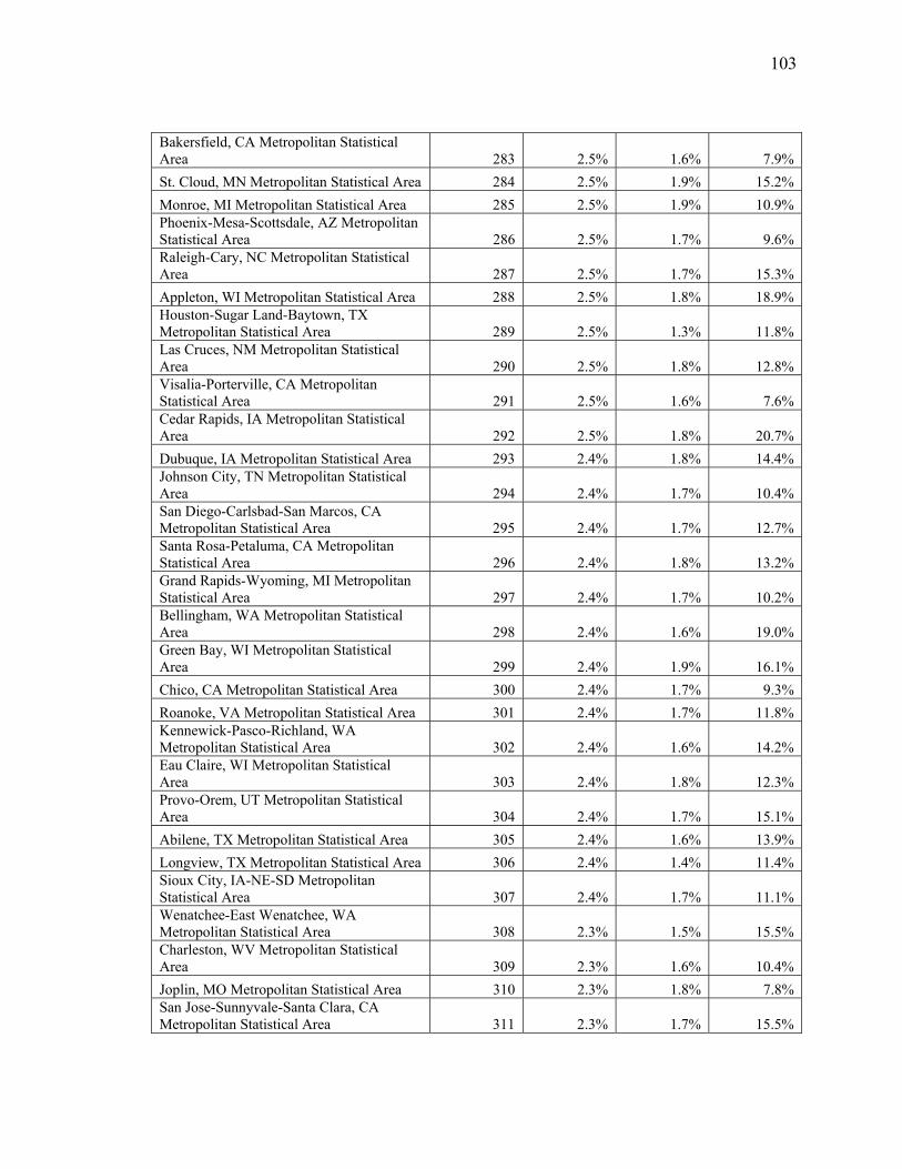
103
Bakersfield, CA Metropolitan Statistical Area 283 2.5% 1.6% 7.9%
St. Cloud, MN Metropolitan Statistical Area 284 2.5% 1.9% 15.2%
Monroe, MI Metropolitan Statistical Area 285 2.5% 1.9% 10.9% Phoenix-Mesa-Scottsdale, AZ Metropolitan Statistical Area 286 2.5% 1.7% 9.6% Raleigh-Cary, NC Metropolitan Statistical Area 287 2.5% 1.7% 15.3%
Appleton, WI Metropolitan Statistical Area 288 2.5% 1.8% 18.9% Houston-Sugar Land-Baytown, TX Metropolitan Statistical Area 289 2.5% 1.3% 11.8% Las Cruces, NM Metropolitan Statistical Area 290 2.5% 1.8% 12.8% Visalia-Porterville, CA Metropolitan Statistical Area 291 2.5% 1.6% 7.6% Cedar Rapids, IA Metropolitan Statistical Area 292 2.5% 1.8% 20.7%
Dubuque, IA Metropolitan Statistical Area 293 2.4% 1.8% 14.4% Johnson City, TN Metropolitan Statistical Area 294 2.4% 1.7% 10.4% San Diego-Carlsbad-San Marcos, CA Metropolitan Statistical Area 295 2.4% 1.7% 12.7% Santa Rosa-Petaluma, CA Metropolitan Statistical Area 296 2.4% 1.8% 13.2% Grand Rapids-Wyoming, MI Metropolitan Statistical Area 297 2.4% 1.7% 10.2% Bellingham, WA Metropolitan Statistical Area 298 2.4% 1.6% 19.0% Green Bay, WI Metropolitan Statistical Area 299 2.4% 1.9% 16.1%
Chico, CA Metropolitan Statistical Area 300 2.4% 1.7% 9.3%
Roanoke, VA Metropolitan Statistical Area 301 2.4% 1.7% 11.8% Kennewick-Pasco-Richland, WA Metropolitan Statistical Area 302 2.4% 1.6% 14.2% Eau Claire, WI Metropolitan Statistical Area 303 2.4% 1.8% 12.3% Provo-Orem, UT Metropolitan Statistical Area 304 2.4% 1.7% 15.1%
Abilene, TX Metropolitan Statistical Area 305 2.4% 1.6% 13.9%
Longview, TX Metropolitan Statistical Area 306 2.4% 1.4% 11.4% Sioux City, IA-NE-SD Metropolitan Statistical Area 307 2.4% 1.7% 11.1% Wenatchee-East Wenatchee, WA Metropolitan Statistical Area 308 2.3% 1.5% 15.5% Charleston, WV Metropolitan Statistical Area 309 2.3% 1.6% 10.4%
Joplin, MO Metropolitan Statistical Area 310 2.3% 1.8% 7.8% San Jose-Sunnyvale-Santa Clara, CA Metropolitan Statistical Area 311 2.3% 1.7% 15.5%

104
Colorado Springs, CO Metropolitan Statistical Area 312 2.3% 1.6% 13.1%
Tyler, TX Metropolitan Statistical Area 313 2.3% 1.4% 12.0% Killeen-Temple-Fort Hood, TX Metropolitan Statistical Area 314 2.3% 1.5% 13.2%
Lincoln, NE Metropolitan Statistical Area 315 2.3% 1.6% 14.9% Lake Havasu City-Kingman, AZ Metropolitan Statistical Area 316 2.3% 1.7% 7.6% San Francisco-Oakland-Fremont, CA Metropolitan Statistical Area 317 2.3% 1.6% 12.7%
Prescott, AZ Metropolitan Statistical Area 318 2.2% 1.5% 11.7% Springfield, MO Metropolitan Statistical Area 319 2.2% 1.7% 10.6%
Napa, CA Metropolitan Statistical Area 320 2.2% 1.6% 11.2% Manhattan, KS Metropolitan Statistical Area 321 2.2% 1.6% 14.5% Great Falls, MT Metropolitan Statistical Area 322 2.1% 1.6% 16.7%
Waco, TX Metropolitan Statistical Area 323 2.1% 1.2% 12.1% Oxnard-Thousand Oaks-Ventura, CA Metropolitan Statistical Area 324 2.0% 1.5% 9.6% Waterloo-Cedar Falls, IA Metropolitan Statistical Area 325 2.0% 1.4% 13.5%
Asheville, NC Metropolitan Statistical Area 326 2.0% 1.5% 11.5% Columbia, MO Metropolitan Statistical Area 327 2.0% 1.4% 13.6% State College, PA Metropolitan Statistical Area 328 1.9% 1.4% 15.4%
Logan, UT-ID Metropolitan Statistical Area 329 1.9% 1.5% 12.0% Duluth, MN-WI Metropolitan Statistical Area 330 1.9% 1.5% 8.2% Minneapolis-St. Paul-Bloomington, MN-WI Metropolitan Statistical Area 331 1.9% 1.4% 11.0% Ann Arbor, MI Metropolitan Statistical Area 332 1.8% 1.3% 11.7%
Victoria, TX Metropolitan Statistical Area 333 1.8% 0.9% 10.6% Cape Girardeau-Jackson, MO-IL Metropolitan Statistical Area 334 1.8% 1.2% 10.6% Charlottesville, VA Metropolitan Statistical Area 335 1.8% 1.3% 11.6%
Billings, MT Metropolitan Statistical Area 336 1.7% 1.3% 15.0% Santa Barbara-Santa Maria-Goleta, CA Metropolitan Statistical Area 337 1.7% 1.3% 8.6%
Lubbock, TX Metropolitan Statistical Area 338 1.7% 1.0% 11.3% Rochester, MN Metropolitan Statistical Area 339 1.7% 1.1% 11.5% Blacksburg-Christiansburg-Radford, VA Metropolitan Statistical Area 340 1.7% 1.2% 10.2%

105
Rapid City, SD Metropolitan Statistical Area 341 1.7% 1.2% 14.9%
Flagstaff, AZ Metropolitan Statistical Area 342 1.6% 1.2% 8.8% Holland-Grand Haven, MI Metropolitan Statistical Area 343 1.6% 1.2% 9.4% Sioux Falls, SD Metropolitan Statistical Area 344 1.6% 1.3% 11.9%
Missoula, MT Metropolitan Statistical Area 345 1.6% 1.2% 13.1% Mankato-North Mankato, MN Metropolitan Statistical Area 346 1.5% 1.2% 7.7%
Corvallis, OR Metropolitan Statistical Area 347 1.5% 1.0% 14.8% Winchester, VA-WV Metropolitan Statistical Area 348 1.5% 1.1% 6.5% San Angelo, TX Metropolitan Statistical Area 349 1.5% 0.8% 10.6%
Iowa City, IA Metropolitan Statistical Area 350 1.4% 1.2% 12.5%
Ames, IA Metropolitan Statistical Area 351 1.4% 1.2% 12.0%
Casper, WY Metropolitan Statistical Area 352 1.4% 1.0% 8.7%
Odessa, TX Metropolitan Statistical Area 353 1.4% 0.8% 6.4% Austin-Round Rock, TX Metropolitan Statistical Area 354 1.3% 0.8% 10.3% Anchorage, AK Metropolitan Statistical Area 355 1.3% 0.7% 9.5% Fort Collins-Loveland, CO Metropolitan Statistical Area 356 1.3% 0.9% 9.0% Fargo, ND-MN Metropolitan Statistical Area 357 1.3% 1.0% 9.5%
Boulder, CO Metropolitan Statistical Area 358 1.3% 1.0% 7.8% San Luis Obispo-Paso Robles, CA Metropolitan Statistical Area 359 1.3% 0.9% 8.0% Cheyenne, WY Metropolitan Statistical Area 360 1.2% 0.9% 10.4% Morgantown, WV Metropolitan Statistical Area 361 1.2% 0.7% 10.7% Grand Forks, ND-MN Metropolitan Statistical Area 362 1.1% 0.7% 9.7% Harrisonburg, VA Metropolitan Statistical Area 363 1.0% 0.8% 5.2% College Station-Bryan, TX Metropolitan Statistical Area 364 0.9% 0.5% 9.1%
Midland, TX Metropolitan Statistical Area 365 0.9% 0.6% 6.2%
Bismarck, ND Metropolitan Statistical Area 366 0.7% 0.5% 9.5%

106
APPENDIX B
INCORPORATED COMMUNITIES IN MIAMI DADE COUNTY
Map reference Incorporated Community Designation Date incorporated Population
2 Aventura City 7-Nov-95 35,762
7 Bal Harbour Village 16-Jun-47 2,513
8 Bay Harbor Islands Town Apr-47 5,628
11 Biscayne Park Village 1933 3,055
28 Coral Gables City 1925 46,780
32 Cutler Bay Town 9-Nov-05 40,286
20 Doral City 24-Jun-03 45,704
13 El Portal Village 7-Dec-37 2,325
34 Florida City City 1914 11,245
3 Golden Beach Town 1929 919
17 Hialeah City 1925 224,669
18 Hialeah Gardens City Dec-48 21,744
33 Homestead City 1913 60,512
9 Indian Creek Village 1939 86
26 Key Biscayne Village 1991 12,344
19 Medley Town 1949 838
24 Miami City July 28, 1896 413,892
25 Miami Beach City 26-Mar-15 87,779
1 Miami Gardens City 13-May-03 107,167
16 Miami Lakes Town 5-Dec-00 29,361
12 Miami Shores Village 2-Jan-32 10,493
21 Miami Springs City 1926 13,809
14 North Bay Village City 1945 7,137
6 North Miami City 27-May-53 58,786
5 North Miami Beach City 1927 41,523
15 Opa-locka City 1926 15,219
31 Palmetto Bay Village 10-Sep-02 23,410
30 Pinecrest Village 12-Mar-96 18,223
29 South Miami City 24-Jun-27 11,657
4 Sunny Isles Beach City 1997 20,832
10 Surfside Town 18-May-35 5,744
23 Sweetwater City 1941 13,499
22 Virginia Gardens Village 10-Jul-47 2,375
27 West Miami City 1947 5,965

107
APPENDIX C
FORECLOSURE PROCESSING STAGES IN FLORIDA STATE
The type of foreclosure process carried out in Florida is known as Judicial Foreclosure
Process where the lender files suit with the judicial system and the property is sold
through auction to the highest bidder. The bidding is carried out by the court or the local
sheriff. It is difficult to estimate the maximum amount of time needed to foreclose on a
business or individual property because it differs from place to place and it depends on
the property being sold. The foreclosure of a property currently takes about 600 days to
run its course from the first notice until the date of sale. Foreclosure process in Florida
begins when you miss out on 3-4 mortgage payment; this usually takes about 6 months
before a Notice for foreclosure will be sent out to the mortgage holder. At this stage the
mortgage holder is late with payment but remain in the property while the foreclosure
proceedings progress. After notice for foreclosure on a property has been received, the
foreclosure process has officially begun. This early stage falls under the pre-
foreclosure period. During the proceedings the mortgage holder receives a Notice of
Default indicating that he/she is late on payment. Notice of Default is a written notice
sent to the mortgage holder by the mortgage lender, it will state how much money is
owed, how late the payment is, and what needs to be done to prevent foreclosure from
happening. Notice of Action is the next step in the foreclosure process. When a mortgage
holder goes further in delinquency and cannot pay the terms stated in the Notice of
Default, a Notice of Action stating the lender’s written demands and their intent to take

108
back the property if the payment is not made is declared. Once the Notice of Action is
posted, the formal foreclosure process takes place.
The lender will then file a Lis Pendens. The term "Lis Pendens" means “litigation
pending” which is the document filed into public record by the lender notifying real
estate and interested parties to the legal claim of a property. This is published on the local
newspaper to put the public on notice that a law suit has been filed against the mortgage
holder. The lawsuit which will be filed under Miami-Dade County where the property is
located will state the intention of the mortgage lender to evict the residents and take over
ownership of the property. The date and time of the auction will be posted and the
property will be sold anywhere from three to six weeks in the future. Up until this point
the mortgage holder is still able to contend for his property if he is able to come up with
the appropriate payment owed to the lender until the set date of auction. Sherriff sale is
the last step of the foreclosure process. This is where the property is auctioned off to the
highest bidder at Miami-Dade county courthouse. Like any auction, the price is low to
begin, but can escalate depending on the location and the demand of the property. Once a
bidder has won the auction for the property, the former mortgage holder has terminated
all of their rights to the property and is evicted after the sheriff sale. The foreclosed
property stays vacant until it is sold to a new permanent owner. Title to the property is
transferred to the winning bidder and the newly purchased property could be vacant for
weeks or months depending on how long it will take the new owner to move in or in
some cases where such properties are bought by a bank or a mortgage company (REO,) it
may be vacant for up to a year until it is rented out or sold to another owner.

109
APPENDIX D
NEAREST NEIGHBOUR ANALYSIS AND SPATIAL AUTOCORRELATION
SUMMARY

110