Special Release for the Buddipole Users Group (Ver. 1.0)This document is provided FREE OF COST for personal or amateur radio club use. Erik Weaver N0EW originally wrote the contents as a series of posts/articles in the Buddipole User's Group. This document may be freely distributed provided the hyperlink information to the current version of this document (www.n0ew.org/book/) and the copyright notice are kept intact; and provided that the document is distributed free of costs. The (copyrighted) cover art is by Erik Weaver.

This work is only partially completed. There is approximately an equal amount of material in various stages of completion to be added to this document at some point in the future. The original series of posts/articles may be found by searching the Yahoo.com Buddipole User's Group (BUG) achieves. However, in the meantime, a number of people have requested a single-volume document in place of the original series of posts to the BUG. Special thanks are extended to James M. "Jim" Geidl, K6JMG for volunteering his time and artwork. Jim not only formatted the main body of this document as a PDF, but additionally took the time to arrange the multiple tables of ASCII-text information into the neatly presented tables you will find herein. He has also rendered the original ASCII-drawings as CAD drawings. Both of which make the text easier, and I trust, more pleasant to read.

My hope is this small booklet will allow those newly entering the exciting world of radio amateur – affectionately called Newbies – to more quickly get up to speed with radio amateur topics while avoiding some of the scraped knees I 'discovered' along my own journey. If you enjoy this text you may also wish to read my KØS “Field Manual.” Both documents are available at: www.n0ew.org/book/

73 – Erik E. Weaver NØEW, October 2ØØ8Springfield, Missouri, USA

Newbie Antenna Woes & Black Boxes By: 73-Erik Weaver n0ew

Newbie Antenna Woes & Black Boxes -- Part I............................................................................. 3 Newbie Antenna Woes & Black Boxes -- Part II ........................................................................... 8

Feed Point Impedance of an Antenna ......................................................................................... 8 Impedance (Z)............................................................................................................................. 8 Complex Impedances.................................................................................................................. 9 Reactance (X).............................................................................................................................. 9

Capacitive Reactance (XC)..................................................................................................... 9 Inductive Reactance (XL) ..................................................................................................... 10

Resonance ................................................................................................................................. 10 Resistance ................................................................................................................................. 10

ii) Ohmic Loss....................................................................................................................... 11 iii) Ground Loss .................................................................................................................... 11 iv) All other Losses............................................................................................................... 11 v) Radiation Resistance......................................................................................................... 11

Line Attenuation ....................................................................................................................... 12 Characteristic Impedance of Transmission Line (Z0) .......................................................... 12 Gain....................................................................................................................................... 12 Forward Wave....................................................................................................................... 13 Reflected Wave..................................................................................................................... 13 Re-Reflected Wave ............................................................................................................... 14 SWR...................................................................................................................................... 14

Newbie Antenna Woes & Black Boxes -- Part III ........................................................................ 16 Looking Into Black Boxes ........................................................................................................ 16 Black Boxes or Black Magyk? ................................................................................................. 16 Black Box Values ..................................................................................................................... 17 Software Used........................................................................................................................... 17 Calculating Wavelength............................................................................................................ 18 Which Wavelength Did We Measure? ..................................................................................... 19 Black Boxes .............................................................................................................................. 20 Black Box #4 (Transmatch) ...................................................................................................... 20 Black Box #2 (XCVR).............................................................................................................. 20

Newbie Antenna Woes & Black Boxes -- Part IV........................................................................ 22 Black Box #3 (Transmission Line) ........................................................................................... 22 Balanced Line ........................................................................................................................... 22 Coax .......................................................................................................................................... 24 Enter the balun .......................................................................................................................... 25 Is this a complete antenna system? ........................................................................................... 27

Newbie Antenna Woes & Black Boxes -- Part V......................................................................... 28 Intro to Transmission Line as an Impedance Transformation Device...................................... 28 What happens inside our transmission line?............................................................................. 29 Here's some important points to remember.... .......................................................................... 30

Characteristic Line Impedance ("Z0") ...................................................................................... 31 Why is this important? .............................................................................................................. 33

Part VI(a) = Transmission Line as an Impedance Transformation Device .................................. 35 Part VI(b) = Transmission Line as an Impedance Transformation Device .................................. 42 Part VII: Antenna Representations & Real Black Boxes.............................................................. 47

Representing Antennas as Component Parts ............................................................................ 47

Newbie Antenna Woes & Black Boxes -- Part I This is a ( hopefully ) brief post directed toward the "new guy on the block" --the warmly welcomed Newbie-- in an effort to help them make a little sense of our extended debate over antennas, antenna "tuning" and the relative merits/demerits of using a transmatch/physically tweaking antenna geometry. A very big bite to be sure! I'll start with two book recommendations: 1. "Reflections II" by Walter Maxwell W2DU. If you see this book, buy it! Then read it once a year for several years. Your book, like mine, will most likely start to fall apart from use. This is a great book written by a NASA engineer. But it is out of print. There have been rumors of a third edition for years now.... still I wait teary-eyed, unfulfilled. 2. "Practical Antenna Handbook" by Joseph Carr. Great book! Most of us end up eventually getting both the ARRL books, "Handbook" and "Antenna Book" because they are good reference materials and everyone cites them. But were I starting out all over, I'd start with the "Practical Antenna Handbook" as my first few reads. It provides a very good base and covers a lot of material. After you read this over a couple times, and digest it, you'll be ready to utilize the two ARRL books as references. OK then. To sum up.... We have three Black Boxes and a fourth Optional Black Box. Black Box # 1 Black Box 1 is the antenna itself. This is normally some combination of metal. Usually wire and/or pipe, but it can be nearly anything made of metal and relatively isolated from its surroundings. But let's assume it is either wire or pipe, and made of metal. We will also limit our discussion to HF antennas, which is to say those intended to be used on one of the bands from 10-meters to 160-meters. Arguably the most basic configurations for HF antennas are the dipole and the 1/4-wavelength ground-mounted vertical antenna with ground radial wires. Other popular contenders would include the inverted-vee, the L, and the vertical dipole. Dipole

This is made from two wires of equal length and orientated horizontally above the earth. The transmission line ( aka feed line ) is connected to the center of the dipole. This is called the feed point. Vertical Dipole Surprisingly, this is a normal dipole pointing straight upward into the sky! ;) It is a standard dipole rotated 90-degrees so that both wires are perpendicular to the earth. Inverted-vee ( Inv-V ) This is a dipole with both ends lower than the middle ( the feed point) and ideally the angle between the two wires shouldn't be less than 90-degrees. Somewhere around 100- to 120-degrees is fairly common. If their angle is increased to 180-degrees it has become a standard dipole. If the feed point is lower than the ends, it is still an inverted dipole, and it will normally work just fine, but this is less common. It is *not* what most people mean when they say "inverted vee." L Take a dipole with a 90-degree angle between the two wires, and turn it so that one wire is parallel to the earth and the other is perpendicular to the earth. This is an "L" antenna. The horizontal wire can be on the bottom or on the top. Like a dipole, the feed point --where the transmission line is attached-- is still where the two wires come closest together. All of the above are basically the same antenna, with slight modifications. In all cases the two wires that make up the antenna geometry can be bent around somewhat to fit available space, or even shortened to a very large degree. As we bend and stretch and otherwise alter the basic geometry of the antenna in question it begins to display somewhat different properties. I think this is to be expected. For now just bare in mind we can alter the basic antenna geometry quite a bit and still end up with an antenna we can make work with the rest of the antenna system. But each time we change something, we most likely will have to make an adjustment elsewhere in the antenna *system* -- the word "system" is important to note. 1/4-wavelength vertical with ground-radial wires This is more wordy to explain clearly. Naturally, there are many variations on a vertical antenna, just as we have already seen with a dipole. But verticals begin with this most-basic "monopole" vertical antenna. The "1/4 wavelength" part means the length of the radiating element is 25% ( 1/4 ) of one full wavelength at that frequency. If we are speaking of 10-meters, nominally that

wavelength is close to 10-meters long. Therefore the 1/4 wavelength vertical would be close to 2.5 meters. Be advised the exact number we would use to cut our wires will *not* follow this simplification. We would calculate from the exact frequency of intended use, and we would then make further adjustments for the real-world vs. the paper theory. For example, as we use thicker wire ( or pipe ) we find we actually shorten the wire somewhat. But don't let details such as these get in the way of seeing the broad picture first. ( I will attempt to delay bringing details into this discussion in the hope of painting a clear picture before muddying the waters with all the details the Devil loves so much. ) The "ground-wires" is referring to what is sometimes called the "missing half" of the antenna. You see, we have ( on paper ) taken a dipole, turned it 90-degrees so that it has become a vertical dipole, and then brutally speared it into the planet earth until it is buried up to its feed point! This, however, destroys the "buried half" so we sometimes call that buried half the "missing" part of the antenna. And even were it intact, it would only be of very limited utility to us because the planet earth acts a lot like a giant RF sponge. In other words, it is a very poor conductor of alternating current at HF frequencies. So we re-create the missing half of the vertical antenna by splaying out a bunch of wire, like spokes in a wheel, with the feed point as their starting point. How many? How far? On, below or above the earth? All these things change the specific type of vertical we are referring to, and each of these is another area of debate. You'll hear all kinds of answers. Ground-radials is the proper term when these radial wires lay on or just below the ground. Of course, if they go too deep they are no longer useful ( spongy earth ). Counterpoise is the proper term if these radial wires are raised a short distance above the ground ( on the order of a few percent of a wavelength ). Ground plane is the proper term when the radial wires are raised very far above the ground, and implies they have been cut to a specific length so as to "resonate" with the vertical, and their number can be greatly reduced, often to as low as two. Black Box # 2 Black Box Two is our transceiver ( XCVR ). Older designs had vacuum tubes inside them, and are called "tube rigs". These also had a impedance matching network inside them which required the "dip and peak" steps to make the antenna system resonate. We will not speak of these older XCVRs very much, but you should be aware they behave differently than the later model IC-based XCVRs. It is these later-year IC-based rigs we normally speak of in our discussions. Tube rigs didn't really care much what they were hooked up to as an antenna. Remember, they had an impedance matching network ( a transmatch ) built into their design. Our IC-based rigs *do* care what they are hooked up to. They have a much smaller range of impedances into which they can

work ( "load into" ) without causing themselves internal damage or entering a self-protection mode and reducing power or shutting off entirely. IC-based rigs I will just call an "XCVR" from now on, and unless I specifically refer to a "tube rig" you can assume that is what is meant. I personally use either an Icom 746 or an Icom 706MKiiG XCVR, but there are many manufacturers at many different price levels available. These "modern" XCVRs are designed to load into (meaning be able to safely transmit at full power into) something close to 50 ohms, with very little reactance. The short-hand for that is: 50 + j0 ohms We are beginning to get ahead of our story. We'll return to this later. Black Box # 3 Black Box Three is whatever we use to connect the other two Black Boxes together. We have Black Box 1 at one end, and Black Box 2 at the other end, and Black Box 3 is connecting them. We call this the transmission line, or the feed line. Ideally it will carry the radio waves between Black Box 1 and Black Box 2 perfectly, never altering the radio waves and never losing any of the radio waves along the way. That looks nice on paper, and it is usually where we begin our discussions to keep things simple, but in the real world neither is true. Transmission line almost always transforms the radio wave along the way to some degree -- this can be a tiny amount or a very large amount depending upon the situation -- and there is always some losses incurred along the way. How much loss depends upon the quality and type of transmission line as well as the length of the transmission line. Black Box # 4 Black Box Four is optional. This is the impedance matching device. It will eliminate any reactance in the antenna system and at the same time transform the resistance of the antenna into something close to 50 ohms, which the "modern" XCVR requires. This Black Box is given a handful of names so as to cause greater confusion ;) These names include: transmatch --my favorite-- antenna tuner, tuner, ATU, auto-tuner, coupler, auto-coupler, matcher, impedance matching network, and several I'm sure to have forgotten or not yet heard. I think the most common is simply "tuner" and even I give in to my large Lazy Bone and call it this at times. We cannot effectively talk about what this Black Box #4 does until we introduce a few other ideas:

1. Resonance 2. Reactance

i) Capacitive ii) Inductive

3. Resistance i) Pure ii) Ohmic loss iii) Ground loss iv) All other losses v) Radiation Resistance

4. Line Attenuation 5. Forward Wave 6. Reflected Wave 7. Re-Reflected Wave 8. SWR

Newbie Antenna Woes & Black Boxes -- Part II Let's define some terms! I can't help but feel much of the trouble we face as radio amateurs lies in poorly defined terms. This is the root cause for much of our disagreements. Since we are a rag-tag bunch of folks, not a professional organization, and scattered across many continents, we end up using terms differently. Is it any wonder we become confused?

Feed Point Impedance of an Antenna This is simply the complex impedance measured where the antenna wires are connected to the transmission line. The transmission line in turn connects the antenna to the transceiver. This complex impedance is usually written in the form: R + jX ohms.

Impedance (Z) When dealing with direct current (dc) we can simply use Ohm's Law: E=I*R; R=E/I; I=E/R. But when we are using an alternating current (ac), such as when we use our transceiver (XCVR) to produce a radio frequency (RF), we must take into account the fact that voltage and current may not peak at the same time. This is because voltage and current are waves traveling along our conductors, moving along as sine waves, and they each travel along our conductors independently. By "independently" I mean they each are free to move along peaking and dipping in exact timing with one another, or they may peak and dip at different times. This relationship of peaking and dipping is called "phase." When they are "in phase" they both peak and dip at exactly the same time. When they peak at different times, they are "out of phase." Aside: Peaking, dipping, and phase, are all based upon a 360-degree circle; as when a bicycle wheel turns. When a circle is stretched out so that one specific point (the reflector, perhaps) on the wheel is tracked along it's path above the street (street = time = the horizontal axis on a graph), a sine wave is created by the reflector when seen by us as the rider rolls past us. Aside: "Dip and peak" has nothing to do with the tuning process of tube-based transceivers. When working with a "pure resistor," the resistance equals the impedance (R=Z), and the simple form of Ohm's Law is preserved. We only need to replace the "R" with "Z": E=I*Z; Z=E/I; I=E/Z. But when voltage and current are out of phase, we are *not* dealing with pure resistance, and the phase difference must be taken into account. This kind of impedance is called "complex impedance." Aside: Here is a link which appears interesting because it includes an online impedance calculator, along with the expressions, and definitions of related terms: http://hyperphysics.phy-astr.gsu.edu/hbase/electric/imped.html

Complex Impedances Complex impedance occurs in an ac circuit when voltage and current are out of phase with one another. But why would voltage and current ever be out of phase with one another? This will happen whenever we run ac through either an inductor (a coil) or a capacitor. When a voltage is applied across an inductor, the coil resists any change in current, and therefore, the current rises more slowly than the voltage. In other words, "current lags voltage." Since ac is an alternating current, the coil is constantly trying to resist the change in the current's direction. This resistance is called "inductive reactance." When a voltage is applied across a capacitor, the voltage is not able to build until positive and negative charges build up on the plates of the capacitor. This charge is created by the current, so current must flow first before the voltage is able to be created. In other words, "current leads voltage." In an ac circuit the current is constantly changing directions and voltage is constantly trying to catch up to the current. This is a form of resistance to an alternating current called "capacitive reactance." Complex impedance exists when we have an alternating circuit displaying both a pure resistance and either inductive or capacitive reactance. The form of the expression we see used most often is: R + jX ohm. The "j-operator" (the "j") is there to remind us that part of the resistance is out of phase. If it is a value greater than zero it is inductive, and if it is less than zero it is capacitive. It is important to remember we cannot add the two halves of this expression together directly. When we measure our antenna systems we must account for two kinds of ohms. One is "pure resistance" and one is "reactance" and when we are using a system with both of these present at the same time, the resulting impedance is called "complex impedance." Since some degree of reactance is normally found in our antenna system it is normal to work with complex impedance.

Reactance (X) Reactance is a form of resistance to an alternating current. One of the big differences between "pure" resistance and reactance, is pure resistance is available to perform work for us. A simple resistor on a circuit board dissipates heat. That is work. The "pure" resistance we seek for our antenna is called "radiation resistance" and it dissipates our RF into the atmosphere. That too is work. However, the power caught up in reactance, of either type, is unavailable to perform work. Instead, it simply cycles back and forth as the alternating current changes direction.

Capacitive Reactance (XC) Capacitive reactance (XC) is created when an excess of capacitance exists in the antenna system. It has a negative sign in front of the j-operator (XC = -jX). It can be removed from the antenna system by adding an equal amount of inductive reactance.

Inductive Reactance (XL) Inductive reactance (XL) is created when an excess of inductance exists in the antenna system. It has a positive sign in front of the j-operator (XL = +jX). It can be removed from the antenna system by adding an equal amount of capacitive reactance.

Resonance This is merely the state of zero reactance. It means the "thing" being measured is purely resistive. That "thing" is normally our antenna. In the ARRL antenna computer modeling course it is defined by Cebik and Straw as less than +/- 1.0 ohm. This means it is a range of complex impedances from +j0.99 ohm on the high end (inductive reactance) to -j0.99 ohm on the low end (capacitive reactance). It is important to note that any antenna will display multiple frequencies for which it is resonant. Remember, resonance only means there is zero reactance. It does *not* have anything to do with the amount of pure resistance present when there is zero reactance. When we speak of a "resonate antenna" we usually mean that frequency for which there is zero reactance and the antenna displays a pure resistance most useful for use in our antenna system. What that value of pure resistance is changes as we change the physical geometry of the antenna wires. For a dipole it is close to 72 + j0 ohms. For a folded dipole it is close to 300 + j0 ohms. For a 1/4-wavelength vertical wire mounted above an extensive system of radial wires it is close to 36 + j0 ohms. This is to say "resonance" isn't one single, immutable thing. Despite our often referring to it as if this were so. Another implied characteristic of a "resonate antenna" is the pattern --or envelop-- created around the antenna by the RF radiating away from it into the atmosphere. I think this is perhaps the most important, and least often mentioned, aspect of a "resonate" antenna. It means that a "resonate dipole" will not radiate directly upwards very well, nor will it radiate off the pointy-ends of its wires very well, but it will radiate very well broadside to its wires. A "resonate vertical" antenna will not radiate directly upwards very well, but it will radiate very well in all other directions (if we discount into planet earth, of course). In fact, provided we can "tune" the antenna, and use sufficiently low-loss transmission line, this RF pattern --or envelop-- is arguably the *only* important aspect of an antenna being resonant! Note the caveat ;) But I am getting ahead of myself. Aside: It should be noted that height above the earth, and objects surrounding the antenna, may all have an effect upon it's feed point impedance, as well as it's RF envelop:. more on these points another time. For now, keep in mind that not only the physical geometry of the antenna, but also its surroundings and it's placement inside its surroundings, all have an effect upon its feed point impedance.

Resistance

This is another term that is often a source of confusion. When we speak of resistance in an antenna system we may be speaking of several sub-types. There are at least five (5) sub-types: i) Pure This means the resistance is very similar to what we see in a standard resistor found on a circuit board. It dissipates the power running through it as heat, or in the case of an antenna as "radiation resistance." When we say "pure" resistance we are also implying there is no reactance present.

ii) Ohmic Loss This simply means the tiny amount of loss occurring as current travels through a conductor:.As electrons knock against one another a tiny amount of power is lost, which I like to think of as a kind of "electron friction." This small loss is always present in a real-world antenna system. Often we can ignore it without unduly affecting our analysis. When modeling antennas or when using transmission line software we can normally choose to work with "lossless" a system, which simplifies the math; or we can work with "real-world" systems that add this loss to the system. This is obviously more realistic, but the math becomes more awkward. Both have their place. It is common to begin analysis while assuming all conductors are lossless, and then to recalculate the analysis with real-world losses taken into account. The results may differ only slightly in some cases, and in other cases be quite significant.

iii) Ground Loss This is RF power lost to planet earth, aka the "ground." It is not normally an important consideration for antennas well above the earth, such as dipoles and ground-plane verticals, but it may be if they remain in close proximity to the earth. It is also very difficult to measure directly, to the point of being impossible for most radio amateurs to measure directly.

iv) All other Losses This, as the name suggests, is any other loss encountered in the antenna system not otherwise specified. It is a catch-all, but it usually does *not* refer to "radiation resistance."

v) Radiation Resistance Radiation resistance is the good stuff! This is the sweet nectar we seek as radio amateurs! Of course, we can't measure this either ;) This is a mathematical construct that is equivalent to the amount of power that would be dissipated by a "pure" resistor that is equal to the power dissipated into the atmosphere. This is why it's the good stuff! This is the amount of RF power we transfer from our antenna system into the sky! Aside: This has nothing to do with what direction that RF power is dissipated, or whether it is being radiated equally in all directions or concentrated in selected directions. Those concerns fall under the term "gain."

Aside: Here are some interesting links, if you like this sort of thing: http://en.wikipedia.org/wiki/Radiation_resistance http://www.w8ji.com/radiation_resistance.htm http://www.arrl.org/tis/info/whyantradiates.html (maybe too much?)

Line Attenuation This is an easy one. This is the amount of power lost in the transmission line. Balanced line (open wire, ladder line, window line, twin lead, etc.) has the lowest loss, and the highest characteristic impedance, of transmission line common to radio amateurs. Coax has much more loss than balanced line, and the amount of power lost rapidly increases as the swr increases. To be clear, it isn't high swr that causes high loss in coax. Rather the high swr is an indicator that tells us the waves traveling inside the coax are bouncing back and forth quite often. Each time the wave travels along the length of the coax it losses a certain amount of power. If that wave bounces back and forth three times, then it loses three times as much power as it did during its first trip. If it bounces back and forth ten times, it loses ten times as much power, and so on. The frequency of the wave traveling along the transmission line is also important. The higher the frequency, the greater the loss per foot traversed. HF causes relatively little loss when compared to 2-meters, which in turn causes relatively little loss when compared to microwave frequencies. For most radio amateur installations RG-213 and its equivalent is pretty effective for HF, and even RG-58 can be used for short runs without suffering extreme losses. But ultimately such decisions are more a matter of opinion than anything else. After all, what is "a lot" or a "short" run? Refer to published charts and tables to determine the loss characteristics of the transmission line you are considering, and cross reference that to the frequencies of intended use, and for the length of line to be used.

Characteristic Impedance of Transmission Line (Z0) This is determined by the physical geometry of the transmission line, and its conductors in relation to one another. Coax is most commonly found in either 50- or 75-ohm characteristic impedance (Z0). Balanced line can range from 300- up to 600-ohms, although 300- and 450-ohm are the most common Z0. There is a special case for transmission line. When Z0 is equal to the complex impedance attached to it, it may be cut to any length and the complex impedance at all points along the transmission line will equal the Z0. The swr will also be "flat" which means a 1.0:1 ratio. This is the condition for which the transmission line will display the lowest loss of RF traveling through it.

Gain

An antenna which radiates equally in all directions has zero gain. An "isotropic" radiator behaves in this manner, but it is only an imaginary construct; an imaginary antenna deep in outer space. One mental image of "gain" is that of a perfectly round balloon with the antenna in the exact center of it -- the isotropic antenna. Now squish-in one side of the balloon, and watch as the opposite end pushes outward. The "gain" has been reduced where you squished it, and increased where it pushed outward. A beam antenna "squishes" the RF radiating from it in this manner. Another way to squish, or deform, this "gain balloon" is to set it on a table and press down on the top of the balloon. This is the shape of the gain produced by a vertical antenna. These "gain balloons" are also useful to help picture the RF envelop radiating outward from the antenna. An important thing to note is that the total power output is the same in all cases, no matter the shape of the balloon. We cannot change the power radiating from the antenna by altering its gain, but we can focus the available power. But focusing power in one direction always comes at the cost of the power from another direction. Gain must also be relative to something. In radio amateur circles the two most common references are the isotropic radiator or the dipole antenna. But we could just as easily have declared an apple cart to be our relative measure, and antenna manufacturers may very be doing so given some of their outlandish claims for gain!

Forward Wave When we transmit, the forward wave moves from our transceiver toward our antenna. This is also called the "incident wave." However, this imagery brings to mind a single wave pushing forward. We often speak of the waves traveling along our antenna system as individual waves, and this if often useful, but do be mindful of the fact that at 28.500 MHz there are 28,500,000 waves moving forward each second.

Reflected Wave When the forward wave meets the antenna feed point one of three things will happen: 1. If there is either an open connection or a short-circuit at the antenna fed point the forward wave will bounce, or "reflect" off it completely, and 100% of the RF power will return toward the transceiver (XCVR). 2. If the complex impedance of the forward wave perfectly matches the complex impedance of the antenna feed point, all of the forward wave will be absorbed into the antenna, and released as radiation from its wires. Of course, if the "antenna" is a "dummy load" the forward wave is still fully absorbed, but not radiated. 3. If the complex impedance of the forward wave is different than the feed point impedance of the antenna feed point --but there is not an open connection, nor a short, at the antenna feed

point-- some of the RF power's forward wave will be absorbed by the antenna, and some of the forward wave will be reflected back toward the XCVR. The amount of power absorbed by the antenna and the amount of power reflected from the antenna feed point depends upon the difference in complex impedance between the forward wave and the antenna feed point.

Re-Reflected Wave The reflected wave travels from the antenna feed point toward the transceiver (XCVR). If there is a transmatch between the reflected wave and the XCVR, the reflected wave will re-reflect off the transmatch. If there is no transmatch between the reflected wave and the XCVR, then the reflected wave will re-reflect off the XCVR. In either case the re-reflection is complete, and none of the reflected power is absorbed by the transmatch/XCVR. The reflected wave re-reflects off the transmatch/XCVR and combines with the newly generated forward wave and moves toward the antenna feed point.

SWR "SWR" means "Standing Wave Ratio." Sometimes it is called VSWR or ISWR. The "V" signifies voltage, and the "I" signifies current. Either will result in the same ratio -- the same value of swr. But voltage is much easier to measure so we most often see VSWR used. I normally just call this "swr" unless there is a specific reason to know whether we are referring to voltage or current as the source of the measurement. Seldom is there such a need. And certainly don't let yourself be bullied by a person flicking "VSWR" or "ISWR" around like a Lyonnais' Blanket (yes, that is a "Charlie Brown" cartoon reference). So what is going on here? What is standing, and why? As the forward waves travel in one direction, and the reflected waves travel in the opposite direction, they combine with one another forming a brand new wave. And if we were able to see their combined sine waves displayed on a screen they would appear to be stationary, despite the fact they are racing past one another like some great electron highway: hence, "standing wave." We then compare their values to one another at the some point on the transmission line and this resulted in a "ratio" of one to the other. Now we have solved the mystery: Standing Wave Ratio - SWR. So we see that swr is just a number. It isn't actually anything, but rather a short-hand comparison of how the forward and reflected waves interact with one another and the greater the value of swr, the greater the difference existing between the forward and reflected waves. While on the subject of swr, please note, low swr, meaning that Siren Song of 1:1, is not required, and sometimes is not even the correct goal! Remember, swr is just a number. It is *not* a meaning, or the be-all end-all of amateur radio! For low-swr all we need is a value of swr low enough for our XCVR to transmit into the antenna system at full power output. Once we achieve

that, any further reduction in swr is normally only a nominal improvement: it is relatively meaningless, but looks pretty on the meter. There just isn't much difference between a swr of 1.5:1 or 1.0:1. If you refer to charts or tables showing power loss for coax at these values of swr you can clearly see this for yourself. (While you have those tables/charts handy, compare the difference between coax and parallel line at, say, 10:1 swr or even 20:1 swr.) However, not all antennas are at their peak performance when a 1.0:1 swr exists. Case in point is the standard 1/4-wavelength vertical monopole antenna over a generous field of radial wires. In this case its ideal antenna feed point impedance is about 36 ohms. Your coax, XCVR, and most other equipment, are all designed to operate at 50 ohms, and 50/36=1.39, or about a 1.4:1 swr. Therefore, in this case, measuring a 1.4:1 swr is your *ideal* goal, not a 1.0:1 swr. And if you achieve a 1.0:1 swr with this antenna it is a *bad* thing! Doing so means there are enough "additional losses" in your antenna system to cause your antenna feed point to appear to be 50 ohms instead of 36 ohms. That means RF power is being lost before it reaches your antenna from which it may radiate into the sky. The lesson here is do *not* kowtow to the 1:1 swr. Figure out what swr you *should* observe, and if you do not, find out why!

Newbie Antenna Woes & Black Boxes -- Part III We've defined most of the terms we'll encounter. Now let's go over a few topics with which we should familiarize ourselves before going into any great detail....

Looking Into Black Boxes We frequently use terms such as "looking into" and "looking toward" when talking about antenna systems and the complex impedance present at various points of the system. We, of course, do not believe our Black Box really has eyes. These phrases are simply a convention to help the reader visualize what we are talking about. It is as if we could stand inside the coax and look down it's length in either direction. Or as if we could peer into the antenna's feed point, or one of the SO-239's on the transceiver or transmatch. So when we say the XCVR is "looking into" the transmission line, we are identifying the complex impedance present at the connection point between the XCVR and the transmission line, and specifically, that impedance which is being delivered to the XCVR from the transmission line. That's a lot or words to use instead of saying "looking into," don't you agree? So this convention results in a much lower word-count. And that is a good thing because as you have no doubt noticed I have difficulty obtaining a low word-count! ;)

Black Boxes or Black Magyk? You can't "trick" an inanimate object. Furthermore, there is no trickery going on in the first place! We live in a physical world ruled by scientifically testable laws of nature. No black magyk; no shamans required. It is my opinion the person crying "trickery!" simply doesn't understand what is happening. As a great author wrote, "any sufficiently advanced technology will appear as magic." Hopefully, we can shed some light on such points of confusion and put an end to such underhanded dealings as tricking our poor transceivers. Besides, the poor transceiver never seems to learn anyway, so leave them alone already! Think of your power supply. It provides something close to 13 volts direct current to your XCVR. Would you say the XCVR is being "tricked" by the power supply? What would you think of the person saying such a thing? You know the process is merely a transformation of power. We input 120 volts ac from the wall, and rectify it to change it into direct current, and use a transformer to step the voltage down to 13 vdc. Sure, there are a number of ways of doing this, and we usually add filtering and whatnot, but these are merely refinements to the basic process of transformation. No tricks. No magyk. The Shaman is unemployed and must brandish his shaky-pokey stick elsewhere.

Our antenna systems are the same. No tricks. No magyk. No Shaman required. We are simply transforming an electro-magnetic wave from one value to another. We do so by manipulating capacitance, inductance, and resistance, as well as how each interacts with the others (meaning whether they are connected in series, in parallel; which is grounded; etc). These variables are what we manipulate inside our Black Boxes to affect the interacting electro-magnetic waves bouncing around inside, and between, our various Black Boxes. The details can become complex at times, but the basic concept is quite simple. We shall find the Black Boxes throughout our antenna system can almost always be reduced to the three-part model already mentioned: an inductor (coil); a capacitor; and a resistor. We then excite this circuit with an alternating current radio frequency (transmit RF through it) and note what happens as a result. That's basically all we are doing.

Black Box Values I'm not talking about whether or not Black Boxes are moral. By "value" I mean the measurements we might take from a Black Box with our test equipment. Let's get out two Black Boxes. In the first we place a series circuit, and in the second we place a parallel circuit. Now hook up your antenna analyzer to these two Black Boxes. If they both provide the same measurement we cannot tell them apart until we look inside the boxes. (There is a $20 word for this which escapes me.) Our antenna system is quite similar -- provided we ignore it radiates RF into the atmosphere. If we make a little box containing some combination of capacitor, inductor, and resistor, and it measures exactly the same complex impedance as our antenna's feed point, we can't tell one from the other simply by measuring them. This means we can model our antenna as some combination of capacitor, inductor, and resistor! We will further find this is true of all our Black Boxes, whether they contain an antenna, a transceiver, transmission line, or a transmatch. Each can be modeled as some combination of capacitor, inductor, and/or resistor, in some physical geometry with one another. This is a critical point, because this is an effective tool for studying complex impedance, and how it changes throughout our antenna system. If you do *not* accept this, stop reading now, and independently research this point. Once you find this to be true, read on.

Software Used Certain parts of our conversation require us to work with complex impedance, and how this changes from one point in our antenna system to another. To determine these values I will use "TransTenna Pro" and "Ham RF Tools" written by Don Cochran, WA0JOW, and/or "EZNEC+" written by Roy Lewallen, W7EL. One could also use the software bundled with the "ARRL Antenna Book" or obtain freeware/shareware software from the Internet. Each piece of software may output slightly different results due to where the software authors rounded their numbers in their calculation, but all the software should be in general agreement.

When thinking about the relative accuracies of predictive software, please recall most of our test and measuring equipment is only about 10% to 20% accurate. Properly calibrated Bird-43 Wattmeters are accepted to be about 7% accurate, and the AIM-4170 Antenna Analyzer has been tested to be about 3% accurate. Furthermore, our software and calculators produce far greater precision than we can ever hope to measure in the field! When you calculate the electrical length of a tuning stub, or the length of an antenna element, you need *not* carry out the calculation to 10 decimal places. Where will you find a cutter capable of that fine of a cut? How would you mount the connectors to that degree of precision? Not to mention, as soon as you spin your VFO off whatever single frequency used in your calculation, that length is no longer accurate, and the farther you spin that VFO the more you increase this inaccuracy. We also have to remember that no matter how well written, no software has yet been developed --nor is anticipated-- that is able to take into account all the variables found operating in the real-world. Real-world variables are all around us and change as our surrounds change. Some changes, like the tour bus parking beside our antenna, are readily apparent to us, while other changes are much more difficult to discern. So don't place too much faith in predictive software. It is a useful tool for guidance, but not a replacement for our reasoning minds and our experiences operating in the field. Software: Don Cochran's (WAØJOW) Software: http://www.pixius.net/~transtenna/index.htm ARRL's TLW and TLA Software: http://www.remote.arrl.org/notes/9043/index.html EZNEC Software: http://www.eznec.com/

Calculating Wavelength We will need to know how to calculate a wavelength at various frequencies. If we only use metric calculations this is pretty simple because the speed of light is roughly 300,000,000 meters per second, and our amateur radio frequencies of interest are expressed in MHz, or millions of cycles per second. Therefore, divide both the MHz and the speed of light by 1-million, and we find the following simple formula: 300 / MHz = Meters For example: 300 / 28.5 = 10.526315789473684210526315789474 Meters (Obviously, an example far more precision than we can ever hope to equal in the field! Can you imagine trying to cut a length of coax to this exact length! Ha!) If you wish to convert this into feet, multiply by 39.37 to get inches, and then divide by 12 for feet: (10.526315789473684210526315789474)*(39.37) = 414.42105263157894736842105263158 Inches (414.42105263157894736842105263158)/12 = 34.535087719298245614035087719298 Feet

Again, much more precision than we can hope to use in the field. A faster way to arrive at what is often an equally useful number of to just multiply the meters by 3.3 (because one meter is roughly 10% longer than one yard): (10.526315789473684210526315789474)*(3.3) = 34.736842105263157894736842105251 Feet An earth-shattering difference of: 0.201754385964912280701754385961 of one foot. To convert the decimal fraction of one foot into inches, just multiply by 12: (0.201754385964912280701754385961)*(12) = 2.421052631578947368421052631532 Inches Just a little less than 2-1/2-inches is the difference between the two methods of converting from X-meters into X-feet at 28.500 MHz. For much field work, this 2.4 inch difference won't matter at all because whatever number we finally arrive at, we add an additional foot or so of length to your antenna elements, and then begin to trim them back until you reach a resonant frequency. Or, if you are like me, you just leave it as is and tune to resonance with your transmatch ;) Either way works just fine. And in neither case does it really matter which of the above practices you follow to convert from meters into feet. Of course, you could just buy a Metric tape measure and avoid all the above entirely ;) But sometimes it is important to be precise. Cutting a tuning stub is an example of this. In such cases run out your calculations to as many decimal points as you can stand, and do not round them until you reach your final number. This will minimize your error. You will also have to measure for an "electrical length" not a "physical length" -- we have been speaking about physical lengths so far.

Which Wavelength Did We Measure? So is the above determining the "Physical" or "Electrical" wavelength? What's the difference and who cares? Radio waves move through space at the speed of light. But they move through a solid conductor, like copper, more slowly, how much more slowly is determined by the physical characteristics of the conductors and its insulators. For transmission line this is called the "velocity factor" --VF-- and is represented as a decimal value, such as 0.66, or 0.90. All reputable manufacturers publish the VF for their transmission line. Much of it is fairly standard by now so there are many sources to look up this information. While each batch of manufactured material may differ somewhat, most of us accept the published values as sufficiently accurate. For those of you with an antenna analyzer there is a process for measuring this value directly, or calculating it from field measurements. Refer to your owner's manual for these instructions. When we discuss wavelength of the radio waves as they move through space, or our atmosphere, we speak in terms of the physical wavelength. When we use transmission line to tune multiple

antenna elements in (or out of) phase, we must use the electrical wavelength. When we tune elevated ground-plane elements, we use the electrical wavelength. When we lay out ground radials on or just under the earth there is no need to fine-tune them (remember the "earth sponge" theory?) so we usually use the physical wavelength. When we are calculating how far 1/2-wavelength is along our coax we must use the electrical wavelength, and at the frequency of interest of course. When we speak of a dipole's height above the earth, we are speaking in terms of physical wavelengths. For Example: What is the wavelength of 28.500 MHz?: 1. Physical wavelength =~ 34.535 feet 2. Electrical wavelength at 0.66 VF =~ 22.793 feet 3. Electrical wavelength at 0.90 VF =~ 31.082 feet (The "=~" means "approximately equal to") From the above we can see there is quite a bit of difference in these measurements, all of which are "correct" from a certain perspective. So if we need to separate two vertical elements of a phased array by 1.0 wavelength, we had better know which is needed (you said, "Electrical" -- right?) and we had better know what kind of transmission line we are using to be certain we used the correct velocity factor!

Black Boxes I'll wrap up this installment by dispatching the two shortest Black Box topics. One Black Box because I don't have much to say about it, and the other because there is far too much to say about it right now! ;)

Black Box #4 (Transmatch) This will be one of the last things we talk about. By the conclusion of our conversation it is my hope this often maligned device will become just another tool at your disposal. However, its operation can be difficult to grasp before understanding the rest of these topics. On the bright side, once you do, it is almost not worth talking about anymore because it's gross operation is defined by these other topics! :)

Black Box #2 (XCVR) I will have little to say about the second Black Box (the transceiver, XCVR). My discussion will be most relevant for those of us using IC-based XCVRs, which is most of us. Those of you with tube rigs are on your own, but I'm confident you are comfortable blazing your own trail. Nor will I spend any time speaking of how to use your XCVR, or various modes. That is all in your owner's manual.

Nearly all of my discussion will end at the output terminal of this particular Black Box. This Black Box must, when looking toward the antenna, see a load close to 50 ohm non-reactive (50 + j0 ohm) in order to safely transmit at full power. The reason for this is 50 ohm coax became ubiquitous after World War II. Had 75 ohm, or 100 ohm coax been the standard, our XCVRs would be designed to load into that impedance. Sorry. There is no deep, dark reason behind 50 ohm radios. There was just a ton of surplus stuff on the market designed for that impedance and it became the de facto standard. There isn't much else we need to know about our XCVR for the purpose of this discussion. If it transmits at full power and no smoke comes out, all is well! ;) Speaking of damaging your XCVR.... Verify whether it has a so-call "self-protection circuit" which will reduce power should the transmitting finals become too hot. If this is true for your XCVR, there is little you can do to damage it, but if this is *not* the case, you need to exercise much more caution than do I. Bare this in mind and observe the precautions your XCVR's manufacturer recommends.

Newbie Antenna Woes & Black Boxes -- Part IV Introduction to Transmission Line and Baluns

Black Box #3 (Transmission Line) Nearly all amateur radio antenna systems require transmission line. One notable exception is a long wire that connects directly to the XCVR's output terminal. This is called an end fed long wire. As the name implies, it is comprised of one long wire, "fed" or connected directly to the output terminal of the XCVR. However, we won't spend any time with this antenna system. Using some kind of transmission line is far more common, and that is the subject of Black Box #3. "Transmission line" derives its name from its primary purpose. We are trying to transmit, or convey, the RF inside it from one location to another with as little loss and as little RF radiation escaping the line as possible. If we do not need to specify which type of transmission line we are talking about, or we already know which we are discussing, we may refer to the transmission line by one of several interchangeable, more generic, names: transmission line; feed line; or just "line." So, what are our transmission line options? For most practical purposes we have two options: balanced line or coax. Both have inherent pros and cons. Balanced line has very little loss but we must be careful where we use it. Coax has much more loss but we can use it almost anywhere. I enjoy using both kinds of transmission line. Ladder line is especially useful in combination with multi-band antennas because they often produce high swr on the line. Coax is often very useful for temporary operations because I can leave it where it falls. I usually carry several different lengths of coax, with connectors suitable for interconnecting these lengths in any combination.

Balanced Line We can connect our XCVR and antenna using two parallel wires running from the XCVR to the antenna. This kind of transmission line is called parallel or balanced line. There are several popular types of balanced line. The oldest is home-made from #12 bare copper wire held about six-inches apart with "spreaders" placed every few feet along its length. These spreaders maintain a constant distance between the two wires and they also serve as electrical insulators. This home-made line usually has an impedance of about 600 ohms, and is called open wire. Commercially produced line is more common. One type is called "window" or "ladder" line. These parallel wires are insulated and their "spreaders" are formed from the same insulating material, with roughly 50% open space between the spreaders. The appearance of open "windows" or "ladder rungs" is the source of its name. When the openings are close to 50% of the area of the line, the name "window" applies, and as these openings increase in area, the name

"ladder" applies. However, people generally call both "ladder line" these days. By whatever name one calls it, we find these come in two popular impedances: 300 ohm and 450 ohm. Those of you old enough to remember putting TV antennas above your home's roof may remember the other popular balanced line. It is called twin lead and it also has insulated wires, but with no open space between them. It is a 300 ohm line. Some people also press speaker wire into service as a balanced wire transmission line. I'll not address improvised line. All balanced transmission line works the same way. The RF travels up one wire and down the other. Since RF is an alternating current and its frequency is on the order of several million cycles per second, each wire generates an electro-magnetic (EM) field around itself. As you may recall from ac theory, two alternating EM waves moving in opposite directions to one another, cancel out one another's radiating EM field. For this reason balanced line radiates very little RF, so long as it's currents remain "equal and opposite" to one another. And that is the sensitive part of using balanced line -- keeping it balanced. Sometimes keeping it balanced is obvious. Laying it on the ground will unbalance it. Laying it on or too close to something metallic or magnetic will unbalance it. Smashing it under your window pane will unbalance it. Sometimes maintaining balance is less obvious. Rain or ice building up upon it can unbalance it. Once I (eventually) remembered the ashtray near my ladder line was made from lead crystal, and this unbalanced the line. Who knew they actually put metal in lead crystal these days! But what does "too close" mean? How close may we route balanced line to a metal window frame or the top of our metal desk? It is easiest to answer this question in terms of widths -- how wide is the balanced line? The home-made 600 ohm is about 6-inches wide. Ladder line can vary from about 1/2-inch to 1-inch, and twin lead is usually a little over 1/4-inch wide. The answer to what is "too close" is expressed in terms of the number of widths of separation between the balanced line and that which may unbalance it. The recommended *absolute minimum* separation is one width, but this is questionable. *Two widths* distance is a better "minimum clearance" standard to observe: once we provide three or four widths distance we have isolation sufficient for most our uses. I would recommend increasing this distance around "active" EM sources, such as electrical lines. Greater distance always equals increased isolation, and in this case, more is better. Greater isolation also exists when the line is run perpendicular to objects that may unbalanced it. Such objects include your antenna, by the way, which is why it is best to route your transmission line away from the antenna so that the line is perpendicular to the antenna. For what distance? As with the clearance to provide balanced line: as far as is practical. Are you getting the idea that working with balanced line is persnickety (requiring painstaking care of detail)? Well, it is, but sometimes it is worth the trouble. When balanced line remains in balance it is one of the best lines you can use, and is one of the lowest loss transmission lines available. So little loss takes place, in fact, that swr isn't even an important consideration! This is why "SWR" wasn't in the radio amateur vernacular until coax came into popular use. Much of it is also lighter in weight than coax, which may be of interest to hikers.

But once balanced line becomes unbalanced, it stops behaving as a transmission line, and instead becomes an active part of the antenna. This means it begins radiating RF. This is in complete opposition to the intended use for transmission line, of course.

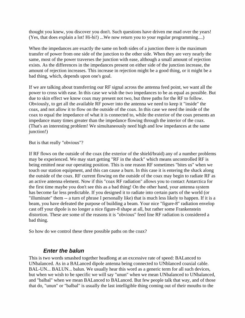
Coax Our other obvious choice is the ubiquitous "coax" cable. It is called coax because, when "looking into" the coax, the two conductors share the same center point -- in other words, they are coaxial. The inner conductor is usually called the "center conductor" and the outer conductor is either called the "shield" or the "braid." The outer conductor can be comprised of multiple layers of metal which form a shield to the outside environment, or it can be a single layer of braided wire. In both cases it creates good separation between the interior conductors and the outside world. This isolation is what allows coax to be routed through walls, behind racks of electrical equipment, through an automobile's firewall, and carelessly coiled up under your feet as you operate at field day. While there are exceptions, for the most part you can treat coax without any regard for how it is routed between your station and your antenna. This is part of coax's popularity. But it suffers much greater loss than balanced line, so it is best to use the highest quality coax you can afford and to use the shortest lengths practical. To more fully understand coax we need to talk a little bit about "skin effect" and the impedance seen at its connection points. As you may recall "skin effect" is a result of an alternating current running across a conductor. Direct current has a frequency of zero. It runs through the entire conductor. This is why we use much thicker wire to power a 100-watt XCVR than a 500-milliwatt XCVR. As we increase frequency (alternating current) the current begins to concentrate on the surface of the conductor. It no longer flows through the interior of the conductor. Once we reach radio frequencies --RF-- the "skin" through which this current travels is so thin that the shielding/braiding of our coax actually behaves as two different conductors on the same piece of metal. How cool is that!? One conductive path is on the interior surface of the shielding/braiding and the other is on the exterior surface. This is one reason we need to understand the concept of impedance. When a junction or connection point exists in a system the power flowing on either side of this junction may be exactly the same, or it may be very nearly the same, or it may be very different on each side of the junction. Which of these is true determines how the two sides of the junction interact with one another. (An additional point: We are *not* going to discuss the difference between a series and parallel junction. They behave in the *opposite* manner to one another: when the series geometry offers rejection, the parallel geometry flows easily, and vice versa. This is not too surprising once you begin to study this, nor is the subject severely complicated. It is just another option when constructing circuits. But we seldom deal with admittance, smho, and the like as amateurs, and never on a casual level. I only mention this so you don't come across this concept at a later date and begin to question how much you

thought you knew, you discover you don't. Such questions have driven me mad over the years! (Yes, that does explain a lot! Hi-hi!) ...We now return you to your regular programming....) When the impedances are exactly the same on both sides of a junction there is the maximum transfer of power from one side of the junction to the other side. When they are very nearly the same, most of the power traverses the junction with ease, although a small amount of rejection exists. As the differences in the impedances present on either side of the junction increase, the amount of rejection increases. This increase in rejection might be a good thing, or it might be a bad thing, which, depends upon one's goal. If we are talking about transferring our RF signal across the antenna feed point, we want all the power to cross with ease. In this case we wish the two impedances to be as equal as possible. But due to skin effect we know coax may present not two, but three paths for the RF to follow. Obviously, to get all the available RF power into the antenna we need to keep it "inside" the coax, and not allow it to flow on the outside of the coax. In this case we need the inside of the coax to equal the impedance of what it is connected to, while the exterior of the coax presents an impedance many times greater than the impedance flowing through the interior of the coax. (That's an interesting problem! We simultaneously need high and low impedances at the same junction!) But is that really "obvious"? If RF flows on the outside of the coax (the exterior of the shield/braid) any of a number problems may be experienced. We may start getting "RF in the shack" which means uncontrolled RF is being emitted near our operating position. This is one reason RF sometimes "bites us" when we touch our station equipment, and this can cause a burn. In this case it is entering the shack along the outside of the coax. RF current flowing on the outside of the coax may begin to radiate RF as an active antenna element. Now if this "coax RF radiation" allows you to contact Antarctica for the first time maybe you don't see this as a bad thing! On the other hand, your antenna system has become far less predictable. If you designed it to radiate into certain parts of the world (or "illuminate" them -- a turn of phrase I personally like) that is much less likely to happen. If it is a beam, you have defeated the purpose of building a beam. Your nice "figure-8" radiation envelop cast off your dipole is no longer a nice figure-8 shape at all, but rather some Frankenstein distortion. These are some of the reasons it is "obvious" feed line RF radiation is considered a bad thing. So how do we control these three possible paths on the coax?

Enter the balun This is two words smashed together headlong at an excessive rate of speed: BALanced to UNbalanced. As in a BALanced dipole antenna being connected to UNblanced coaxial cable. BAL-UN... BALUN... balun. We usually hear this word as a generic term for all such devices, but when we wish to be specific we will say "unun" when we mean UNbalanced to UNbalanced, and "balbal" when we mean BALanced to BALanced. But few people talk that way, and of those that do, "unun" or "balbal" is usually the last intelligible thing coming out of their mouths to the

average bear's ear, perhaps because balbal is so similar to babble? Or maybe this is only one of my many personal limitations? ;) So we have this balun.... what do we do with it? There are two pieces to this part of the puzzle: the coax and balun itself. One job we expect a balun to perform is suppression of feed line radiation. For the coax to keep the RF inside the coax, as compared to the antenna's feed point impedance, the exterior of the coax's shield has to present a very large impedance to its conductors on the interior of the coax. How much greater? Opinions seem to vary. Some say three or four times, others say at least ten times as great impedance on the shield as at the feed point. It is difficult to arrive at a perfect answer because the antenna feed point varies quite widely, especially on multi-band antennas. This leads to a number of conflicting reports from well-meaning fellow radio amateurs. But if you have an excessively large difference --more than you "need"-- there is no harm. So too much impedance on the exterior of the coax is safe to use, just like vitamin C. Recall that when impedance is a close match on both sides of a junction (connection), power flows across the junction easily. If that junction happens to be from the antenna feed point to the exterior of the coax shield, this is generally undesirable for the above reasons. So as we increase this impedance difference the RF is more likely to remain inside the coax, which is what we normally desire. This is one duty the balun performs for us. The other job we sometimes expect a balun to perform is a transformation of impedance. Examples of this are the 4:1 balun, and the 2:1 balun. The first thing to note about these is that phrase "4:1" or "2:1" is shorthand, not literal. The balun is actually designed for a specific ratio, such as 200:50 ohms in the case of most so-called 4:1 baluns, and 100:50 ohms in the case of common 2:1 baluns. Other ratios are possible, and the TRSB sold by Buddipole is an example of this. It provides three switch-selectable impedance ratios: 1:1, 2:1, and 4:1. But it is designed as a step-up transformer. The 1:1 is a straight-through 50:50 ohm transformation. The 2:1 is stepping the impedance up from 25 ohms to 50 ohms, and the 4:1 is stepping up from 12.5 ohms to 50 ohms. As we stray from the balun's designed ratios it begins to work less effectively. This is *not* to say is stops working altogether. In many cases it remains quite serviceable. But if it gets hot to the touch or worse yet, cracks, then you know you are over-stressing the balun. Technical details aside, the purpose of the balun in this case is as a type of step-up or step-down transformer. If we are using 50 ohm coax at some point in our antenna system --which we almost always use at the XCVR-end of the system-- and the opposite end is operating at a much different impedance the use of a transforming balun is logical. If we are using an antenna with higher feed point impedance than 50 ohms, such as some loops, a folded dipole, or most multi-banded antennas for example, we may benefit from stepping down their impedance before the radio waves enter the coax. If we are using an earth-mounted vertical, which has lower feed point impedance that 50 ohms, we may well wish to step this up before the radio wave enters the coax. But stepping up/down the antenna's feed point impedance is not a requirement. Sometimes we prefer to use a 1:1 balun and only concentrate upon eliminating feed line RF radiation. To determine how much this will help us we have to consider the extra loss in the coax caused by

swr in excess of 1:1. If this results in a large amount of additional loss we may benefit from using a step up/down transformer (balun), but if the additional losses are quite small --perhaps because we are using balanced line-- there is little to be gained by doing so. Later we'll discuss how to calculate this additional loss due to swr. For now, just keep in mind there is no one "right" answer that fits every antenna system. (This is a good rule of thumb to remember anytime you are discussing antenna system options.)

Is this a complete antenna system? With the addition of the transmission line connecting the XCVR and the antenna, these first three Black Boxes *may* form a complete antenna system. It is a question of comparing impedances throughout the antenna system. If all impedances are close enough to one another these are the only Black Boxes we need to build a complete antenna system. Therefore, if our antenna happens to be resonate near 50 + j0 ohms, and we are using 50 ohm line, we are done. If our antenna is resonate at some multiple (or fraction, as with the TRSB) of 50 ohms, we can add a transformation balun (4:1, 2:1, etc) to match the line impedance where needed. So with the addition of one or more simple baluns, the antenna system is complete. The idea is to use standard 50 ohm coax to connect to your XCVR, and at the antenna-end of the system we use whatever transmission line offers suitable impedance and also meets the needs of the environment (coax vs. balanced line). Where the impedances are different at the connection points, we may insert a transformation balun. If we successfully transform the antenna's feed point impedance to 50 + j0 ohms by the time it reaches the XCVR, using just transmission line and/or baluns, we are done. If not, we have some additional impedance matching to do, which is discussed as Black Box #4, the transmatch.

Newbie Antenna Woes & Black Boxes -- Part V

Intro to Transmission Line as an Impedance Transformation Device

It's time to discuss Black Box #3: transmission line. Understanding transmission line is critical because anytime we study how the other Black Boxes interact within our antenna system, we must take into account the "impedance transformation" created by our line (assuming transmission line is used and that we desire an accurate answer). I use the software program "TransTenna Pro" to simulate the complex impedance throughout the antenna system. We may choose either "losses" or "real-world" transmission line. Quite often we start with lossless line, which sometimes makes the problem easier to understand, and then we repeat the study with "real" line, which always has some loss. If we know the antenna feed point impedance, and we want to know what value this impedance is transformed into at the XCVR-end of the transmission line, we enter the length of the transmission line, it's attenuation, and velocity factor; from this input the unknown complex impedance at the XCVR is calculated. Or we can reverse the process and enter a known XCVR impedance and see what that is transformed into at the antenna-end of the transmission line (at the antenna feed point, where the line and antenna are connected together). The transmission line behaves the same regardless of which end we hook up to the XCVR, therefore, we can look into it in either direction with equal accuracy ;) We may also study how impedance changes along the length of transmission line. For example, to find the impedance at four equal distances along a 50-feet piece of coax, we divide 50 by 4 (50/4=12.5) and run four simulations, changing only the length of the line each time: 1/4-length = 12.5-feet; 1/2-length = 25.0-ft; 3/4-length = 32.5-ft; and the entire length = 50-feet. When we return to study the whole 50-foot piece of coax we now know what the impedance is at each of these points along the line. (Recall there is a difference between a line's physical length, which never changes, and it's electrical length, which changes each time we alter the frequency being transmitted through the line. By the way, the same is true of your antenna elements: physically they remain the same length, but electrically they change their percentage of wavelength each time you change frequency. This is why a "resonate" antenna is no longer resonate once you change frequency.) So this software allows us to determine the complex impedance at any point along our transmission line, and as seen from either direction (looking into the line toward the antenna or toward the XCVR). We can determine this impedance for either end of the line, or at any point along the line. We tell the program from which end we are starting, whether to use real or lossless line, and how far down the line to calculate the impedance (by specifying the length of the line to equal each distance we wish to examine). If the complex impedance never changes along the length of the line from one end to the other, no impedance transformation is taking

place. However, if the complex impedance does change, the line is in fact an impedance transformer, and if this is true, we may sometimes wish to alter the length of the line to "tune our antenna." (We'll discuss this concept later, and in greater detail, for now, just warm up to the possibility.) Aside: A similar software program, TLW ("Transmission Line for Windows"), is provided with purchase of the "ARRL Antenna Book." Additionally, a Google search should provide a variety of freeware/shareware programs suitable for studying transmission line transformation. Many "Smith Chart" study guides are also available. The various software programs simply automate the process of generating and interpreting a Smith Chart.

What happens inside our transmission line? This depends! To what it is connected? If we transmit into a perfect antenna system, a sine wave of RF races from our XCVR at nearly the speed of light, through the line, and hits the antenna feed point (where the line is connected to the antenna elements), where it finds a perfect impedance match so it zips right in -- the RF wave is fully absorbed by the antenna and radiates into the sky! YAY! Mission accomplished! :) But this is unusual. Normally the antenna system is *not* perfect. Or if it was perfect, we messed it up by changing frequency and it is no longer perfect. (See how we are? We actually expect our antenna to perform well across a *range* of frequencies!) In the not-perfect (i.e. usual) case, we transmit and that RF wave races down our transmission line, as optimistically as before, and slams into the antenna feed point. But this time it is *not* a perfect match! Instead an "impedance mismatch" exists. Some of the RF still gets past this mismatch and is absorbed by the antenna (unless the connection is a dead-short or completely open). But the rest of the RF wave bounces off the antenna feed point --it is "reflected"-- and races back through the line toward the XCVR. When this "reflected wave" hits the XCVR it is re-reflected (100%), joins up with some brand new RF, and together they race through the transmission line toward the antenna, starting this process (cycle) all over again. This keeps happening the entire time we transmit, literally millions of times per second. If there isn't a perfect impedance match where the transmission line is connected to the antenna, RF bounces (reflects and re-reflects) back and forth between the XCVR and the antenna: back and forth, over and over again, until we stop transmitting. And when we use "real-world" line some RF is lost during each trip up the line, and some more lost each trip back down the line. (A similar series of events is taking place inside the XCVR. When the transmitter fails to "see" suitable impedance into which to transmit, an impedance mismatch is created. Some of the transmitted RF gets past this mismatch and enters the antenna system, and some interacts inside the transmitter, which is where "bad things" may happen -- overheating transmitting finals for one. This is why "too high swr" has gotten a bad name. This is despite swr merely being just a number --a concept-- it's not real at all! As such, it cannot impart any effects upon our equipment. To believe otherwise is like believing the number 13 will bring you bad luck. Poor swr, so wrongly maligned!

That said, however, "too high swr" is sometimes an indicator signaling the existence of a very real underlying condition which may damage our equipment. This is how swr gets it's bad name, why it isn't harmful at all, yet why it may signal harmful conditions, which is how it got it's bad name.)

Here's some important points to remember.... Recall the value of swr is created by the interaction between the forward transmitted wave and the reflected wave. It is the ratio of one RF wave to the other. SWR is just a number. SWR is like a tornado siren: it cannot damage your home, it merely alerts you a harmful condition may exist. Once RF leaves the XCVR it has only two options:

• It will be radiated in the sky, no matter how many times it has to bounce back and forth to escape the antenna system;

• Or it gets changed into heat, warming the line. ("Transmission line attenuation" is the $5

phrase for this conversion into heat.) That's it. It never re-enters the XCVR. It never "disappears" into nothingness, although if there are other elements in the antenna system, most notably coils, these too may "warm up" and add their own RF loss. You see, all conductors offer some "friction" to electrons. This is true whether the conductor is a transmission line, a transmatch, a loading coil, an antenna wire, or a circuit board inside your XCVR. Usually these losses are small --although in some cases they are large-- and usually they offer us something of value in exchange for their added loss to the antenna system. How much is "too much loss," and "is it worth the trade," are opinions; you'll just have to learn a bit about what is happening, weigh what you gain against what you lose and make up your own mind. As operators, we have two choices: ...We can effect a change upon the impedance of the RF wave racing toward the antenna in such a manner that it equals the impedance at the antenna's feed point, and is fully absorbed by the antenna; ...Or we can let it "fracture" upon striking the antenna feed point, causing some of the RF to be absorbed by the antenna and some of the RF to be reflected back toward the XCVR. These are our only two choices. However, I should point out the impedance match need not be "perfect" for us to have a very serviceable antenna system, transmitting at full power, and suffering very minor RF loss. So "close enough" is often quite good. The sharp reader will note this determination is again opinion-based ;) If we choose to effect the impedance in the antenna system, there are many ways we may do so! We may change the physical geometry of the antenna. We may change it's height or it's surroundings. We may add some inductance (a "loading coil") or add some capacitance (a "top

hat," aka "capacity hat" or "cap hat"). We may add some combination of inductance, capacitance and resistance at some point in the antenna system (a "transmatch," aka "antenna tuner," "tuner," or "ATU," among other names). Or, we may add --or subtract-- some length of transmission line. This last option is what we're going to play with now. What we choose to use for transmission line plays an important role in determing what happens between the time the RF leaves the XCVR and the time it strikes the antenna's feed point. The transmission line is made of material which is more dense than the vacuum of outer space, therefore the RF travels more slowly through the line. In space it travels at the speed of light. Through the line it travels at some fraction of this speed, and that fraction is called the "velocity factor" (VF). Balanced line is typically on the order of 85% to 95% VF while coax is generally around 66% to 75% VF. If the transmission line were "perfect" --zero "electron friction"-- it would have a VF of 100% and the wavelength of the physical and electrical waves would be identical. In real-world line, the electrical wavelength is always shorter (because it is slower, due to "electron friction") than the physical wavelength. And the electrical wavelength is always shorter by exactly the VF percentage. In addition, real line has some loss --called "attenuation"-- which converts some of our RF into heat. Real line also adds some capacitance to the RF wave. All of these factors result in a measurable change taking place to our RF wave as it travels from one end of the line to the other. With one exception, that is....

Characteristic Line Impedance ("Z0") All transmission line has a "characteristic impedance" ("Z0") which is sometimes called the "surge impedance." But what determines the characteristic impedance of transmission line? Z0 --the "ohms" of the line-- is determined by the size of the conductors, the distance between them, how much insulation is used, and from what material the insulation is made. Fortunately all these variables have long since been figured out for us. We can look up the formulas and do the math for ourselves, or we can assume the data published by the manufacturers is correct, or we can use an antenna analyzer to measure the impedance of the line we are using. Usually we use published data. Unless we have a need to be extremely precise this is close enough. But if we need to be super-precise we had better measure the line we are using, because while the published data is reasonably accurate there may be variations between manufacturer's batches. So what about this "special case" for transmission line? Should both ends of the transmission line be connected to an impedance identical to the Z0 of the line, for all points along the line, the complex impedance is equal to the Z0. This means when our transceiver (XCVR) is transmitting a RF wave at 50 +j0 ohms into a transmission line with a Z0 of 50 ohms, which is in turn connected to an antenna (or "load") of 50 +j0 ohms, all of the RF is absorbed by the antenna, there are no reflected waves, and we can "look into" the line at any point between the XCVR and the load, in either direction, and always see the same complex impedance, which in this example will always be 50 Ohms.

Below is an example using "perfect" or lossless transmission line. The line lengths chosen range from a short 2-foot line, much like we would use as a "jumper" cable to interconnect some of our station equipment, all the way up to an insane 1,000-foot length of transmission line. That is like buying a full reel of coax and just putting connectors on each end of the line! - TABLE ONE: Lossless Line - Line Length in Feet: 1000 100 34 20 10 2 Frequency (MHz) Frequency (MHz) 28.5 28.5 28.5 28.5 28.5 28.5 Generator (XCVR) Impedance: Generator (XCVR) Impedance: Real (Ohms) 50.0 50.0 50.0 50.0 50.0 50.0 Imaginary (Ohms) 0.00 0.00 0.00 0.00 0.00 0.00 Transmission Line: Transmission Line: Electrical Wavelength Electrical Wavelength 28.9 2.89 0.98 0.57 0.29 0.05 Characteristic Impedance.. Characteristic Impedance.. 50.0 50.0 50.0 50.0 50.0 50.0 *VF *VF 100% 100% 100% 100% 100% 100% *Attenuation/100-Ft (db) *Attenuation/100-Ft (db) 0.00 0.00 0.00 0.00 0.00 0.00 *Matched Line Loss (db). *Matched Line Loss (db). 0.00 0.00 0.00 0.00 0.00 0.00 *Loss Due To SWR (db)... *Loss Due To SWR (db)... 0.00 0.00 0.00 0.00 0.00 0.00 *Total Line Loss (db)... *Total Line Loss (db)... 0.00 0.00 0.00 0.00 0.00 0.00 Load (Antenna), Real Part.. Load (Antenna), Real Part.. 50.0 50.0 50.0 50.0 50.0 50.0 Load (Antenna), Imaginary.. Load (Antenna), Imaginary.. 0.00 0.00 0.00 0.00 0.00 0.00 VSWR at the Generator VSWR at the Generator 1.00 1.00 1.00 1.00 1.00 1.00 VSWR at the Load VSWR at the Load 1.00 1.00 1.00 1.00 1.00 1.00 Where: MHz = MegaHertz. Load = Antenna. VF = Velocity factor. Z = Impedance. Z0 = Characteristic impedance of the transmission line. "XCVR" = "Generator" = Transceiver. This is sometimes called the "Source" or "Signal Source." "Lambda" = the Greek letter that looks like an upside down "Y" means "wavelength" in our context; or a sine wave of one period. "Imaginary" = "reactance." Aside: I don't personally believe "imaginary" is a good term to use so I avoid its use. However, you should be aware that some people refer to reactance as being "imaginary" power. It is quite real of course, as we discussed earlier. My recommendation is should you hear someone call reactance "imaginary" hear it as "reactance" in your head; and be on guard. Maybe they are just using the term loosely and the rest of what they have to say is correct, but then again, maybe they are confused. (There is a lot of that going around our ham radio circles, and using wrong terms or proper terms improperly all add to our collective confusion.) What can we discern from the above? Obviously we are using theoretical "lossless" line. Note that for each line beginning with the "*" there are no losses. With real-world transmission line there is always some loss. It may be a very small loss, but it is always present even under the best of conditions. Therefore, this line is an imaginary construct and we cannot exactly duplicate the results in the real-world.

What else? The impedance of the load and the generator never changed. It doesn't matter whether we look into the line from the end connected to the XCVR (generator), or from the end connected to the antenna (load). This is a result of the "special case" of the Z0 matching both the generator and the load. In such cases, no matter where we might cut the line and measure the complex impedance, we find it is the same and it is always the same value as the line's characteristic impedance (Z0). This will be true no matter what length of line we use. (Except that real-world line always suffers some losses along the length of the line, although they are quite small under perfectly match conditions.) If you inspect the above table closely you will see the only thing to change is the electrical wavelength, or the "Lambda," of the physical length of the line (measured in feet). This is the *only* thing that changed no matter what length of coax we measured.

Why is this important? When using a modern XCVR and 50 ohm coax, if we adjust the antenna's physical geometry and/or environmental surroundings so that it presents a 50 +j0 ohm load to the antenna-end of the coax, we do not need to do anything else to "tune" the antenna system. This may mean less gear to carry up a mountain. It may mean getting a "broken" antenna system back on the air during an emergency. Or it may just be something we do for fun. Whatever the reason, it is one method of many to tune an antenna system. It is also the only case where the length of the 50 ohm line is unimportant in terms of impedance transformation (because there is none). You still can't use 1,000-feet of RG-174 and expect to hear anything, of course, but if you are using less than 100-feet of coax of reasonable quality, all things being equal, you should be in pretty good shape. Recall that when the entire antenna system is operating at the same Z0 as the transmission line, swr is flat (1:1) and there will be as little line attenuation (loss) as is possible. This isn't really much of a concern when using balanced line, but it may be quite important when using coax. We will return to this point in greater detail when we talk about "tuning the antenna." Aside: "Tuning" simply means removing reactance from the antenna system -- which is also called a "resonate" antenna system. Any reactance within +/- 1.0 ohms is considered to be "resonant" by the authors of the "ARRL Antenna Modeling Course," Dean Straw N6BV and L.B. Cebik W4RNL (SK). I personally consider any reactance within +/- 10 ohms to be a moderate amount of reactance, meaning it is easily offset in most cases, or doesn't greatly detract from antenna performance. As we continue to increase reactance we encounter increasing difficulty in offsetting it, and our antenna system increasingly suffers. In the past I have found reactance values within +/- 100 ohms to often be successfully offset. However, it is difficult to provide a hard and fast rule regarding an acceptable value of reactance prior to "tuning" because the value of pure resistance present is also an important factor in this decision. Your surroundings also play an important role. For example, it is much more difficult to tune an antenna inside your living room than in the middle of an open field.

Recall that "resonate" only means zero reactance. This may happen at many different values of pure resistance, and even a "resonant" 100 ohms will offer our XCVR a 2:1 swr, which may cause some XCVRs to reduce transmitting power. It is also worth noting that all antennas have multiple "resonate" frequencies. We normally overlook this and only mean the frequency within our radio amateur band(s). (Unfortunately, this too is too common. Often it isn't what you are being told that creates poor understanding, but rather all the things "everyone knows" but never bothers to tell you!)

Part VI(a) = Transmission Line as an Impedance Transformation Device We've set the table in our earlier discussions, so this time we'll go short on theory and long on examples. Yay! :) Transmission line theory is valid for all antenna systems, of course, so this discussion is valid for any antenna using transmission line. We will start with a plausible antenna and proceed to cut apart the coax and see what impedance is inside it at various distances from the antenna. A Buddipole (www.buddipole.com) portable dipole antenna with fully extended "black" whips is modeled at 28.500 MHz using EZNEC+ (ver.5.0) antenna modeling software, which predicts the feed point impedance as 63.68 - j 44.05 ohms (we'll round this to 64 - j44 ohms). This is the complex impedance present where the antenna and transmission line connect where the swr is reported as 2.2:1 (for a 50 ohm system). The complex impedance and swr at the opposite end of the transmission line is dependent upon the length, and type, of line. For most IC-based XCVRs a 2.2:1 swr is a little too high because most XCVRs reduce their transmitting power when exceeding a swr of 2:1. So our first goal is to lower the swr at the XCVR-end of the transmission line. The complex impedance starting at the antenna feed point is almost always different by the time it travels down the line to the XCVR. If we successfully change (transform) the antenna impedance into a near-resonate 50 ohm load (50 +j0 ohm) at the XCVR's output terminal, the swr at the XCVR will be 1:1, which in turn allows the XCVR to safely transmit into the transmission line/antenna at full power, whether that is 100-watts, 5-w, or 500-mW. (Well, since I've said "1.0:1 swr" we'd best address this obsession. Most XCVRs work perfectly well with a swr of 1.5:1, so in most cases a 1.5 swr is operationally as good as a 1.0 swr. For some XCVRs this is true of a 2:1 swr. Determine your swr-goal by referring to your XCVR's manual. In addition, most of our radio amateur metering equipment's accuracy is at best +/- 3% and +/- 10% to 20% is much more common. So don't obsess about obtaining a 1.0:1 swr. Instead take logical steps to keep efficiency high throughout the antenna system, and once your XCVR may transmit at full power, consider your job well done.) Now, there are many ways to achieve a near-resonate 50 ohm load (impedance match) for our XCVR. But the method we are going to examine is simply using different lengths of coax between the antenna and XCVR. *Constant change* is the normal condition for complex impedance measured along our transmission line between the antenna feed point and the XCVR. The antenna feed point creates a certain complex impedance where the line connects to it. As we "look into" the line moving from the antenna toward the XCVR we see the complex impedance undulates --rises and falls in a repeating rhythm-- along its entire length. The number of full and/or partial cycles is dependent upon the "electrical" wavelength of the line. If the line is long enough we will see a series of impedance "highs" and "lows" occurring in regular intervals. These highs and lows gradually make lower-highs and higher-lows (funneling together). If the transmission line is very short we

will only see a fraction of one cycle. By carefully selecting the length of line we may determine the complex impedance presented at the XCVR-end of the line (but only within the range of undulating impedance highs and lows). Do you recall the "special case" for transmission line? When the antenna, transmission line and XCVR are all operating at the same impedance, the impedance is the same everywhere along the line. That is the only condition for which the above "undulation" is untrue. Therefore, by changing only the length of transmission line, we discover the antenna's feed point impedance is transformed (changed) when it arrives at the XCVR. Using a 25-foot length of coax between our antenna and XCVR will present the XCVR a certain complex impedance into which to load; and replacing the 25-foot piece of coax with a 30-foot piece of coax will provide the XCVR a different complex impedance as its load. Alternately, the same change in impedance may be achieved by simply adding a 5-foot piece of coax to the original 25-foot piece of coax. This process of altering the length of the line is how we may use coax to "tune" our antenna. This, however, does not mean we can use any coax to "tune" any antenna system to resonance near 50 ohms. The antenna feed point generates a given complex impedance where it connects to the transmission line. From this starting point the complex impedance (Z) will range up and down, but for only a certain amount in either extreme. Impedance (Z) values beyond this range are out of reach unless we make some further change to the system (we will not discuss such changes at this time). In addition, as the length of the line becomes greater the extreme values of Z will slowly decline to an average value. This is to say, the highest-high and lowest-low in the first cycle will be of a greater magnitude (farther from the average value) than cycles farther along the line. This "dampening" effect is due to line attenuation (RF loss). A picture is surely worth 1,000-words, but since this is a text document let's look at some table data and talk about the highlights.... Comparison of 50-Foot Line Lengths: Transmission Line Lossless RG-58/U RG-213/U Input Data Freq MHz........... 28.500 28.500 28.500 (Identical) Antenna Z0 ..REAL Part (ohms) 64 64 64 (Identical) ..Reactance (ohms) -44 -44 -44 (Identical) Transmission Line ..Z0............... 50.0 53.5 50.0 (Note RG-58/U) ..VF............... 100.0 66.0 66.0 (Note Lossless) ..Atten/100-Ft (dB) 0.0 2.4 1.1 (Different) ..Length.(Feet) 50.00 50.00 50.00 (Identical) Calculated Output: "What the XCVR sees"

Z at the XCVR ..Real Part (ohms) 104.940 30.898 25.186 See Note 3 ..Reactance (ohms) -21.850 +4.872 +3.490

VSWR: ..Generator (XCVR) 2.215 1.753 1.998 See Note 2 ..Load (Antenna) 2.215 2.128 2.215 Transmission Line (dB): ..Matched Line Loss 0.000 1.200 0.550 ..Loss Due to SWR 0.000 0.267 0.159 ..Total Line Loss 0.000 1.467 0.709 Wavelength (Lambda) 1.448 2.194 2.194 See Note 1 Where:

• Lossless: This line is a theoretical construct. It has zero loss, so zero RF power is lost in the coax. It cannot exist in the real world.

• Z: Means complex impedance, expressed as "R + jX Ohms". • Antenna Z: This is the complex impedance present at the point where the transmission

line and antenna are connected. It is in two-parts, real and reactance. • Antenna Z, REAL Part: This is the "pure resistance" part of the complex impedance (the

"R" part). • Antenna Z, Reactance: This is the "reactive" part of the complex impedance (the "jX"

part). • Reactance: This means "resistance to an alternating current" (such as RF). Negative

values designate capacitive reactance; Positive values, inductive reactance. • VF: Velocity Factor. How much slower electrons travel in the line vs. the speed of light,

expressed as a percentage. • Atten/100-Ft: The attenuation of the line, per 100-feet. Expressed in dB (decibels) of loss. • Length: Length of the transmission line, in feet. • Z at the XCVR: This is the complex impedance where the transmission line is connected

to the XCVR. • VSWR, Generator (XCVR): This is the swr "seen by" the XCVR, at the XCVR, looking

into the coax toward the antenna. • VSWR, Load (Antenna): This is the swr "seen by" the Antenna, at the antenna feed point,

looking into the coax toward the XCVR. • Matched Line Loss: This is the "best case" loss in the line due only to attenuation. Both

the XCVR and antenna are assumed to be at the same non-reactive impedance as the characteristic impedance (Z0) of the line. This is the least amount of loss possible, under ideal conditions.

• Loss Due to SWR: This is the "additional loss" created as a direct result of swr. Each time the RF wave travels the length of the line some of the RF is converted into heat ("line attenuation"). As swr increases, so does the "additional" loss, because higher swr means the RF waves must "bounce" (or "reflect" and "re-reflect") more often before either escaping out the antenna, or being converted into heat. So, the greater the ratio of swr, the greater the number of "trips" and therefore the greater the accumulated losses.

• Total Line Loss: The sum of the two aforementioned losses. • Wavelength (Lambda): When using "lossless" line the physical and electrical lengths are

identical. When using real-world line, this is always the *electrical* wavelength of the line, at the frequency specified, and it is always different than the physical line length.

Lambda will change when we change frequency, or when we alter the physical length of the line.

Note 1: This is the "Lambda" which is a $5 word meaning the wavelength of one full period (cycle), much like a single sine wave. In the above table, calculations are based on a 28.500 MHz frequency, along a 50-foot length of coax for each type of line. Recalling the formula to calculate the length of a single wavelength... 300/MHz = Meters 300/28.5=~ 10.5263 meters How many feet is this? (10.5263 meters) * (39.37 inches) / (12 inches) =~ 34.5351 feet Now, how many of these wavelengths (at 28.5 MHz) are in our 50-feet of coax? To find out, divide the length of the coax by the length of one wavelength: (Length of coax)/(One full wavelength) = Number of this wavelength within the length of coax specified. 50/34.5351 =~ 1.448 *physical* wavelengths 1.448 is the number of wavelengths calculated by our software for lossless line of a 50-foot length. But does it make sense? If you have been playing around on 10-meters very long you should recall one full wavelength is somewhere around 34- or 35-feet, depending upon the specific frequency, of course. And 35 will divide into 50 roughly 1.5 times (50/35=~1.43), so yes, this does make sense. (Always question your results. If they seem bizarre, double-check your calculations and your premise.) Now we know 34.5-feet is the approximate length of a single wavelength at 28.5 MHz traveling through outer space. Recalling that our RF wave travels more slowly through a physical conductor than in outer space, we'd expect to see the real-world coax display a greater number of wavelengths through the same 50-foot piece of coax. This may be difficult to picture at first. Basically, in outer space there is nothing to slow down the wave, so it stretches out to its full length. But should that same wave try to move through a solid object --flow along the surface of a conductor-- it encounters resistance, and this slows it down somewhat. (The percentage of "slow down" is the Velocity Factor, VF.) So when we stand back and compare the same wave moving through different materials, we see it is more or less "compressed" depending upon which material it is

moving through. This "compression" is caused by how much or how little resistance that material offers to the wave. -- Wave Traveling --> Outer Space (100% VF): ~~~~~~~~~~~~~~~~~~~~ 90% VF: ~~~~~~~~~~~~~~~~~~ 50% VF: ~~~~~~~~~~ This is in fact what we see. RG-58/U completes 2.194 wavelengths in 50-feet; RG-213/U also completes 2.194 wavelengths because RG-58/U and RG-213/U both have a 66% VF. Any transmission line with a different VF will complete a different number of wavelengths for the same 50-feet of distance. RG-8/U, for example, has a VF of 78%, therefore it must display a different number of wavelengths for the same physical length of line:

Freq. MHz VF-% Dist. Lambda (WL) 28.500 100 50 ft 1.448 WL in Outer Space 28.500 78 50 ft 1.856 Electrical WL 28.500 66 50 ft 2.194 Electrical WL So we see that for a given piece of transmission line, the length of that line as measured in wavelengths is dependent upon only two facts: 1. Frequency of the RF; and 2. Velocity factor (VF) of the line. Anytime you change either of these, you change the length of the line in terms of it's electrical wavelength. Meanwhile, it's physical length --as measured with a tape measure-- remains the same. We normally change the physical transmission line much less often than we change frequency. This means the coax remains physically unchanged, but "how long the line looks to the RF" is dependent upon the frequency of the RF. This is one of the reasons our antenna system behaves so differently on different bands. Note 2: Lower swr is always better, right? Isn't this one of the most commonly heard mantras in radio amateur circles?

Lossless line and RG-213/U share nearly the same values of swr. We see RG-58/U has lower swr than either RG-213/U or lossless line, and it drops more as it moves from the antenna to the XCVR. What does this mean? RG-58/U is the better coax? But how can it be better than "lossless" line? Each of these points is related to the RF loss caused by the line (attenuation). Lossless RG-58/U RG-213/U VSWR @ Generator (XCVR) 2.215 1.753 1.998 VSWR @ Load (Antenna) 2.215 2.128 2.215 Here our problem has only one variable: the type of transmission line being used. All other conditions are identical, therefore all changes must be caused by our choice in line. As its name implies, lossless line has zero loss, so it's value of swr is as perfect as we could hope to duplicate. When we measure the swr right at the antenna feed point it is 2.215. And when we measure the swr 50-feet away from the antenna it is an identical 2.215, for a net loss of zero. But we live in the real-world where our coax does suffer RF loss. Unlike "lossless" line, our coax converts some of our RF into heat. One way to observe the effects of this RF loss is as the difference in swr from one end of the coax to the other end of the line. The longer the line, the greater this RF loss. And the lower the swr. RG-213/U measures 2.215 swr at the antenna feed point. But 50-feet later it measures 1.998 swr. The lower value of swr is caused by RF lost to the coax as heat. A net loss of 2.215-1.998= 0.217. RG-58/U measures 2.128 swr at the antenna feed point. It starts at a different swr because its "Z0" is 53.5 ohms, not 50.0 ohms like lossless line and RG-213/U. At the other end of the 50-foot length of RG-58/U its swr is reduced to 1.753. A net loss of 2.128-1.753= 0.375. Compared to RG-213/U, RG-58/U lost more of its RF to the line as heat, which is why its swr is lower for the same physical length of line. So this is a case when *higher* swr is "better" because the higher swr indicates more of the RF remains available to radiate out of our antenna. This means *sometimes* low swr is a good thing. But sometimes high swr is a good thing. So we must know when to expect low swr, and when to expect high swr. (And, of course, we have to define "low swr" and "high swr" because these are qualitative terms not quantitative values.) So the question "is my swr low enough?" is malformed and misses the point. We aren't looking for "low swr" -- we are looking for a value of swr that changes as little as possible from the *ideal* swr for the type of antenna system we are measuring. When we don't see the expected change in swr, we need to figure out what is wrong with our antenna system. This is a more complex question, but it ultimately yields a more useful answer.

Note 3: This is the complex impedance seen by the XCVR. We know it started out as 64 - j44 ohms at the antenna feed point. By the time the RF travels along the entire length of the coax to the XCVR it is changed -- transformed. But the individual values do not seem to share any rhyme or reason? Or do they?

Lossless RG-58/U

RG-213/U

Z at the XCVR: ..Real Part (ohms).= 104.940

30.898 25.186 See Note 3

..Reactance (ohms).= -21.850

+4.872 +3.490

Shall we retrieve that Shaky-Pokey Stick we threw away and try to "trick" these numbers? ;) The problem is we just don't have enough information to make sense of what we are seeing. This is a snap-shot. We need a movie!

[Part VI is too long, so I've broken it into two sub-parts, (a) and(b)

Part VI(b) = Transmission Line as an Impedance Transformation Device We will get more information --build each frame of our movie-- by chopping up our coax into smaller pieces and see what is happening at intervals along the entire length of the line. So I'm going to start with a very short length of coax, and show you what impedance "pops out" the other end, where the XCVR is connected. Then we'll add a little more coax and see what pops out, and so on. By the time we replicate our 50-foot length of coax the above table should make sense. Recall we have our initial forward RF wave moving up the line from the XCVR toward the antenna. When it hits the antenna feed point at the end of the coax, some RF goes into the antenna and some reflects back toward the XCVR. This reflected wave passes through the next forward wave making its first trip to the antenna. As the forward and reflected waves pass through each other they form a new wave --called the "standing wave"-- which is merely the sum of the instantaneous values of the two passing waves. The complex impedance that "pops out" where the XCVR is connected is the result of the interaction between the forward and reflected RF waves. For example --using completely made-up and meaningless numbers-- if the forward wave has a value of +5 and reflected wave a value of -2, they sum to a value of +3. If the next instant along the line they have respective values of +6 and +1, they sum to +7, and so on. Now, let's look at some real-world coax, and proceed with our dissection... RG-58/U: ------- MHz = 28.500; Antenna Feed Point Impedance = 64-j44 ohms; Coax: Z0= 53.5; VF=66%; Attenuation/100-Ft=2.4 dB; --------------------------------------------------------------------- -Antenna Feed Point Impedance is 64-j44 Ohms and Looking Toward XCVR- --------------------------------------------------------------------- RG-58/U Length|Results at XCVR:....Transmission Line (dB):

Feet.. Lambda Real + j (Ohms) VSWR MatchLoss +swrLoss TotLoss Notes: 0 0.000 64.0 -j 44.0 -na- ----n/a-- ---n/a-- --n/a-- 1-inch 0.004 61.6 -j 43.6 2.13 0.00 0.00 0.00 6-inch 0.022 51.5 -j 40.4 2.12 0.01 0.00 0.02 [4] 1 0.044 42.4 -j 34.9 2.11 0.02 0.01 0.03 2 0.088 31.7 -j 22.6 2.11 0.05 0.01 0.06 2.85* 0.125 27.3 -j 12.4 2.10 0.07 0.02 0.09 4 0.175 * 25.6 +j 00.9* 2.09 0.10 0.03 0.12 [2,5,6] 5.70** 0.250 31.1 +j 20.5 2.07 0.14 0.04 0.18 6 0.263 33.3 +j 24.1 2.07 0.14 0.04 0.19 8 0.351 68.6 +j 41.9 2.05 0.19 0.06 0.25 8.55* 0.375 86.2 +j 37.5 2.05 0.21 0.06 0.26

9.6 0.421 *109.1 +j 01.0* 2.04 0.23 0.07 0.30 [1,5,6] 10 0.439 *105.3 -j 16.8 2.04 0.24 0.07 0.31 [1] 11.40*** 0.500 64.2 -j 40.8 2.02 0.27 0.08 0.35 [3] 12 0.526 50.4 -j 37.1 2.02 0.29 0.08 0.37 14 0.614 29.5 -j 14.8 2.00 0.34 0.09 0.43 14.25* 0.625 28.6 -j 11.9 2.00 0.34 0.09 0.44 15.3 0.671 * 26.9 -j 00.2* 1.99 0.37 0.10 0.47 [2,5,6] 15.4 0.676 * 26.9 +j 00.9* 1.99 0.37 0.10 0.47 [2,5] 16 0.702 27.7 +j 07.5 1.99 0.38 0.10 0.49 [4] 17.10** 0.750 32.4 +j 19.8 1.98 0.41 0.11 0.52 18 0.790 40.9 +j 29.8 1.97 0.43 0.12 0.55 19.95* 0.875 84.5 +j 33.8 1.95 0.48 0.13 0.61 20 0.977 85.9 +j 33.0 1.95 0.48 0.13 0.61 21 0.921 *104.1 +j 00.8* 1.95 0.50 0.13 0.67 [1,5] 22 0.965 * 86.6 -j 31.7 1.94 0.53 0.14 0.67 22.80*** 1.000 64.3 -j 37.8 1.93 0.55 0.14 0.69 [3] 24 1.053 42.0 -j 29.4 1.92 0.58 0.15 0.73 25 1.097 32.9 -j 18.6 1.92 0.60 0.15 0.75 [7]

RG-58/U Length|Results at XCVR:....|Transmission Line (dB):...|

Feet.. Lambda Real + j (Ohms) VSWR MatchLoss +swrLoss TotLoss Notes: 25.65* 1.125 29.8 -j 11.5 1.91 0.62 0.16 0.77 26 1.141 * 28.8 -j 07.7 1.91 0.62 0.16 0.78 [2] 26.7 1.171 * 28.1 -j 00.2* 1.90 0.64 0.17 0.80 [2,5] 28 1.228 30.9 +j 13.7 1.89 0.67 0.17 0.84 28.50** 1.250 33.7 +j 19.1 1.89 0.68 0.17 0.86 30 1.316 51.1 +j 33.5 1.88 0.72 0.18 0.90 31.35* 1.375 82.7 +j 30.6 1.87 0.75 0.19 0.94 32 1.404 * 96.7 +j 14.6 1.87 0.77 0.19 0.96 [1] 33.4 1.421 * 99.7 +j 00.6* 1.86 0.78 0.19 0.97 [1,5] 34 1.492 69.1 -j 34.7 1.85 0.82 0.20 1.02 34.20*** 1.500 64.3 -j 35.1 1.85 0.82 0.20 1.02 [3] 36 1.579 37.0 -j 22.0 1.84 0.86 0.21 1.07 37.05* 1.625 31.0 -J 11.0 1.83 0.89 0.21 1.10 38 1.667 * 29.3 -j 01.2 1.83 0.91 0.22 1.13 [2] 38.1 1.672 * 29.3 -j 00.1* 1.83 0.91 0.22 1.13 [2,5] 38.89** 1.750 34.9 +j 18.3 1.81 0.96 0.23 1.18 40 1.755 35.6 +j 19.4 1.81 0.96 0.23 1.19 42 1.843 63.6 +j 33.3 1.80 1.01 0.24 1.24 42.73* 1.875 80.6 +j 28.1 1.80 1.03 0.24 1.26 43.8 1.922 * 95.7 +j 00.4* 1.79 1.05 0.24 1.29 [1,5] 44 1.930 * 95.1 -j 06.0 1.79 1.06 0.24 1.30 [1] 45.59*** 2.000 64.3 -j 32.5 1.78 1.09 0.25 1.34 [3] 46 2.018 56.1 -j 31.8 1.78 1.10 0.25 1.36 48 2.106 34.1 -j 15.1 1.76 1.15 0.26 1.41 48.44* 2.125 32.2 -j 10.7 1.76 1.16 0.26 1.42 [2] 49.5 2.172 * 30.5 -j 00.1* 1.76 1.19 0.27 1.45 [5] 50 2.194 * 30.9 +j 04.9 1.75 1.20 0.27 1.47

RG-58/U Length|Results at XCVR:....|Transmission Line (dB):...|

Feet.. Lambda Real + j (Ohms) VSWR MatchLoss +swrLoss TotLoss Notes: 55.2ft 2.422 92.2 +j 00.3* 1.72 1.33 0.29 1.61 [5]

60.9ft 2.672 31.6 -j 00.1* 1.69 1.46 0.31 1.77 [5,7] 66.6ft 2.922 89.1 +j 00.1* 1.67 1.60 0.33 1.92 [5] 72.3ft 3.172 32.7 -j 00.0* 1.64 1.74 0.34 2.08 [5] 78 ft. 3.422 86.2 +j 00.0* 1.61 1.87 0.36 2.23 [5] 83.7ft 3.672 33.7 -j 00.0* 1.59 2.01 0.38 2.38 [5] 89.4ft 3.922 83.7 -j 00.0* 1.56 2.15 0.39 2.54 [5] 95.1ft 4.172 34.7 -j 00.8* 1.54 2.28 0.40 2.69 [5] 106.5 ft 4.672 35.7 +j 00.1* 1.50 2.56 0.43 2.98 [7]

--SWR at XCVR "Improves" w/ Length-|-Loss Increases w/ Length-|------

1. By glancing at the first 25-feet of coax, we immediately see there are impedance maximums approximately 11-feet apart. If this is truly a repeating cycle we should find additional "highs" roughly every 11-feet. Looking at the second 25-feet of coax (26- through 50-feet) we see these highs appear as expected. We also see their magnitude is diminishing. Line attenuation is causing this, and it is expected.

2. The repeating cycles of lows are a little more difficult to see, but they are also present.

The first low appears 4-feet down the line from the antenna, and is followed by the second low near the 15-foot mark. So the lows also appear to be following an 11-foot repeating cycle. If so, we would expect additional lows in 11-foot intervals. While these intervals are not perfect, we see additional lows appearing as expected. (If we continued to divide our line into smaller and smaller pieces our "rough" intervals would become more refined, and the regularity of the highs and lows should become more precise.)

3. Standard transmission line theory tells us we should see the antenna feed point

impedance repeat every 1/2-wavelength. This means we should see a complex impedance close to 64 -j 44 ohms at 0.5, 1.0, 1.5, and 2.0 wavelengths. For the most part, we do. The line attenuation causes some degradation in the impedance, especially to the reactance, but overall it remains relatively unchanged.

4. Occasionally we see some of our figures are "off" due to rounding. But the larger trends

are more important to us right now than great precision. And what are these trends? We see all losses increase with the length of the coax. We see swr continues to drop as we add more coax. And we see rhythmic patterns to the RF waves traversing the coax -- both the highs and the lows repeat regularly as their values are slowly declining in magnitude. (If we make the coax long enough the RF waves will eventually "flat line." So at exceedingly long lengths, transmission line behaves as a "dummy load" and the swr becomes a nearly perfect 1:1 since RF no longer reaches the antenna, having been entirely converted into heat).

5. Resonance also repeats rhythmaticaly. We find that the reactance has become resonant

each time we reach a "high" or "low" point (see notes [1] and [2], above). These are the lengths for which the length of transmission line has made the antenna resonate to the XCVR. "Resonance" means zero reactance, which in turn means all the power put into

the antenna system is available to perform useful work. This is why we favor "resonant" loads for our XCVR.

Upon closer inspection, we see our resonate choices fall into two groupings. We may attempt to match the XCVR to the impedance "highs," or to the impedance "lows." However, none of these present a near-50 ohm resonant load so we won't find a 1:1 swr. Even so, when the transmission line presents the XCVR a non-reactive, purely resistive load the impedance match may still be "close enough" to 50 ohms. How close is "close enough" is dependent upon the XCVR.

This begs the question: do the impedance highs, or lows, offer us a better impedance matching opportunity? The next block of lines displays the resonate lengths of coax for easier comparison: 0- to 25-feet of Coax:

Feet Impedance Highs Impedance Lows SWR dB Loss 9.6 109.1 +j01.0 n/a 2.04 -0.30 21 104.1 +j00.8 n/a 1.95 -0.67 4. n/a 25.6 +j00.9 2.09 -0.12 15.3 n/a 26.9 –j00.2 1.99 -0.47

26- to 50-feet of Coax:

Feet Impedance Highs Impedance Lows SWR dB Loss 33.4 97.7 +j00.6 n/a 1.86 -0.97 43.8 95.7 +j00.4 n/a 1.79 -1.29 26.7. n/a 28.1 -j00.2 1.90 -0.80 38.1 n/a 29.3 –j00.1 1.83 -1.13 49.5 n/a 28.1 –j00.1 1.76 -1.45

51- to 75-feet of Coax:

Feet Impedance Highs Impedance Lows SWR dB Loss 55.2 92.2 +j00.3 n/a 1.72 -1.61 66.6 89.1 +j00.1 n/a 1.67 -1.92 72.3 n/a 32.7 –j00.00 1.64 -2.08 60.9 n/a 31.6 –j00.1 1.69 -1.77

76- to 100-feet of Coax:

Feet Impedance Highs Impedance Lows SWR dB Loss 78.0 86.2 +j00.0 n/a 1.61 -2.23 89.4 83.7 –j00.0 n/a 1.56 -2.54 83.7 n/a 33.7 –j00.0 1.59 -2.38 95.1 n/a 34.7 –j00.8 1.54 -2.69 106.5 n/a 35.7 +j00.1 1.5 -2.98

There is not much difference between the high or low impedances close to one another. The biggest change comes as a result of adding more coax, which slowly reduces the difference between the highs and lows while reducing the swr. Of course, as we add line, we add loss. Such is our choice. We are able to match the antenna's complex impedance to the XCVR by adding line until we reach a value of impedance that results in an acceptably low swr, but in some cases we may have to use a longer length of coax than we prefer. So, is it worth using 60- or 70-feet of coax, and accepting a 2 dB loss, to drop the swr below 1.7? Is it worth using over 80-feet of coax, and adding nearly 3 dB in line loss, to give the XCVR a swr below 1.6? Does either choice offer a "low enough" swr for your XCVR to safely transmit? Only you can answer these questions. But maybe it is worth the additional loss if that is the only way to obtain a suitable load for the XCVR. Or perhaps not if you have the option of tweaking the antenna elements, or a transmatch, to obtain a match with less RF loss. I'm not trying to tell you *what* to do. I'm just sharing a variety of options with you, and showing you what is going on behind the scenes. *You* decide which is best for your purposes.

6. I also note other wavelength intervals (in 1/8-wavelength increments) just in case you

wish to examine the table for additional cycles. Looking for repeating rhythms of impedance in your transmission line will help you develop a feel for what is happening inside the line, and is time well spent.

One such cycle of interest is how a 1/4-wavelength change in line length --in either direction-- imparts a large change upon the complex impedance. This may be useful when we can't quite obtain an impedance match. (As frequently occurs when using an internal transmatch, which are well-known for their limited impedance matching capability.) By shifting the line length in either direction by up to 1/4-wavelength we sometimes raise or lower the complex impedance sufficiently to permit an impedance match. This is why people sometimes suggest carrying additional lengths of line equal to 1/8- and 1/4-wavelengths. The logic is similar to using 1/2-wavelength pieces of coax, except instead of closely reproducing the impedance this attempts to maximize the *change* in impedance. The Cliff Notes are 1/2-wavelength intervals of transmission line tend to duplicate the line impedance, and 1/4-wavelength intervals of line tend to maximize the change in impedance. (Later we'll discuss this in greater detail.)

7. We see that RF loss (attenuation) has reduced the swr to 1.92 at the end of a 25-foot

length of RG-58/U coax. This means some XCVRs will be able to load into this antenna as is, while other XCVRs will require additional swr reduction. If we require a swr of 1.7 or lower, that arrives at any line length in excess of 61-feet. If we require a 1.5 swr or lower, we must use at least 106.5-feet of RG-58/U, but we also incur a 3 dB loss in power (half our transmitted power is dissipated into the line as heat) as previous noted.

Part VII: Antenna Representations & Real Black Boxes The time has arrived to examine the Black Box containing the antenna itself. When we first hear about "antennas" most of us think we need only know what kind of antenna to use, or discover which is the "best" antenna, and naturally enough, we assume the only reason to use an antenna is to communicate. But this obviously isn't always true -- a dummy load serves as a perfect example. It is designed specifically to *not* communicate! Yet it remains a useful tool and it is a type of antenna, or more properly, a "load" for our antenna system. (An antenna is merely one kind of "load" for the XCVR.) When don't we need, or even want, a "real" antenna? Such occasions include designing an impedance matching network, troubleshooting an existing antenna system, or predicting the radiation patter of an antenna system. At such times the antenna's importance is secondary to the interactions taking place around it. Our concern is representing the antenna in such as way that we better understand how it interacts with other important elements of the antenna system or the environment. These elements may be close at hand, such as creating tuning stubs or designing an impedance matching network, or these elements may be quite distant from our station. We may wish to identify optimal take-off angles to communicate with (or "illuminate") a specific part of the planet, or we may wish to identify and compare gain and null bearings of several antennas. At such times we obviously have no need for a dipole cut for resonance at some random frequency. We do need a simple and effective means of representing our antenna in graphical or mathematical terms. We will discuss those representations we radio amateurs most commonly use. These uses generally fall into two groups. The first group helps us work out impedance problems and may involve transmission line, antenna feed point impedance, and impedance matching networks. When working out impedance problems we are concerned with complex impedance (R+jX ohms) and specific components, their values, and possibly how to physically connect one to another. The second group helps us visualize how our antenna system interacts with the world around us. These drawings graphically indicate where the antenna displays gain (strong signals) and nulls (low or no signals) both in the vertical ("elevation") and horizontal ("azimuth") dimensions. When figuring out where our antenna "talks" and where our antenna is "deaf" we are concerned with such matters as take-off angle, gain, and nulls in the RF pattern radiating from our antenna.

Representing Antennas as Component Parts The main reason we use this kind of drawing is to simplify the problem at hand so we can quickly and easily evaluate all the component parts and how they may interact with one another. Often our primary concern is complex impedance changes throughout the antenna system. We use icons, or symbols, to indicate various parts and often insert component values in the drawing.

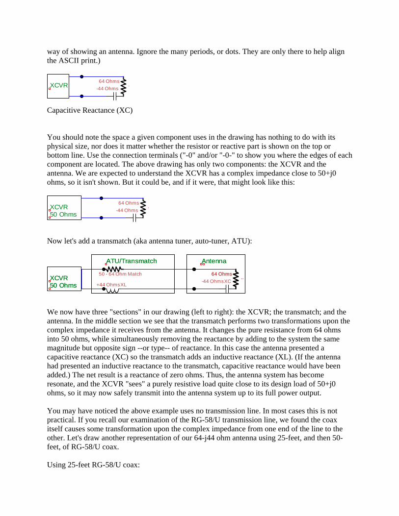
In some cases the component placements and connections are to be taken literally, in some cases they are abstract, and sometimes we combine both depictions in the same drawing. The more common components found in these drawings are the resistor (which often indicates the antenna, or load, and less frequently indicates the Ohmic resistance of the conductors), capacitors and inductors (sometimes representing physical components and sometimes representing the type of reactance present), connection or soldering points (also called "terminals"), and the ground (typically an earth ground or a chassis ground). Let's start with a simple dummy load. A properly designed dummy load presents the XCVR a load very close to a purely resistive 50 ohms (50 +j0). It has one or more resistors inside it. All conductive leads are kept very short so as to minimize stray inductance or capacitance, ideally resulting in zero reactance across all the frequencies for which it will be used. Antenna represented as a zigzag symbol for a resistor Common antenna resistance is 50 Ohms.

50 Ohms

.. Remember the basic Buddipole dipole antenna used in these examples has 64 ohms resistance plus 44 ohms of capacitive reactance, which we express mathematically as 64-j44 ohms. :

64 Ohms

..

-44 Ohms

(Capacitive Reactance) If the antenna were instead 64 ohms resistive plus +j44 ohms inductive reactance, it would look like this:

64 Ohms

..+44 Ohms

(Inductive Reactance) The XCVR is shown as a sine wave inside a circle. It is often called the "Generator" or the "Source." Sometimes it is simply labeled "XCVR." (~). Putting all this together, a basic antenna system might be drawn as follow. (The "zzz" is an attempt to indicate a zigzag line typically used to indicate a resistor -- which is another common

way of showing an antenna. Ignore the many periods, or dots. They are only there to help align the ASCII print.)

64 Ohms..

-44 OhmsXCVR

Capacitive Reactance (XC) You should note the space a given component uses in the drawing has nothing to do with its physical size, nor does it matter whether the resistor or reactive part is shown on the top or bottom line. Use the connection terminals ("-0" and/or "-0-" to show you where the edges of each component are located. The above drawing has only two components: the XCVR and the antenna. We are expected to understand the XCVR has a complex impedance close to 50+j0 ohms, so it isn't shown. But it could be, and if it were, that might look like this:

64 Ohms..

-44 OhmsXCVR50 Ohms

Now let's add a transmatch (aka antenna tuner, auto-tuner, ATU):

-44 Ohms XCXCVR+44 Ohms XL50 Ohms

64 Ohms..

50 - 64 Ohm Match

ATU/Transmatch Antenna

XCVR50 Ohms

64 Ohms..

ATU/Transmatch Antenna

We now have three "sections" in our drawing (left to right): the XCVR; the transmatch; and the antenna. In the middle section we see that the transmatch performs two transformations upon the complex impedance it receives from the antenna. It changes the pure resistance from 64 ohms into 50 ohms, while simultaneously removing the reactance by adding to the system the same magnitude but opposite sign --or type-- of reactance. In this case the antenna presented a capacitive reactance (XC) so the transmatch adds an inductive reactance (XL). (If the antenna had presented an inductive reactance to the transmatch, capacitive reactance would have been added.) The net result is a reactance of zero ohms. Thus, the antenna system has become resonate, and the XCVR "sees" a purely resistive load quite close to its design load of 50+j0 ohms, so it may now safely transmit into the antenna system up to its full power output. You may have noticed the above example uses no transmission line. In most cases this is not practical. If you recall our examination of the RG-58/U transmission line, we found the coax itself causes some transformation upon the complex impedance from one end of the line to the other. Let's draw another representation of our 64-j44 ohm antenna using 25-feet, and then 50-feet, of RG-58/U coax. Using 25-feet RG-58/U coax:

-44 Ohms XCXCVR+18.6 Ohms XL50 Ohms

64 Ohms..

50 - 30.9 Ohm Match

ATU/Transmatch AntennaCoax

30.9 Ohm Match

-18.6 Ohms XCXCVR50 Ohms

64 Ohms..

ATU/Transmatch Antenna

Above we see four "sections" in our drawing (left to right): the XCVR; the transmatch; the transmission line; and the antenna. We are not depicting the (normally) short coax jumper connecting our XCVR and transmatch. Since the impedance is a purely resistive 50 ohms at this point in the antenna system we may expect it to remain largely unaffected over the length of this jumper. The antenna intercepts passing RF waves traveling through the atmosphere, and this induces a current along the antenna which arrives at the antenna feed point with a complex impedance of 64-j44 ohms. From here the RF wave enters the coax, and travels along the 25-feet of coax in the direction of the XCVR. The complex impedance of the RF wave is transformed as it moves along the coax and it arrives at the transmatch with a complex impedance of 32.9-j18.6 ohms. The transmatch performs two simultaneous transformations upon the RF wave. It steps up the 32.9 ohms of pure resistance to 50 ohms pure resistance while it adds +j18.6 ohms of inductive reactance (XL). Adding +j18.6 ohms XL to -j18.6 ohms XC, results in a net reactance of zero ohms (thus creating resonance). These two transformations together create a complex impedance of 50+j0 ohms on the XCVR-side of the transmatch. The short piece of jumper coax delivers this to the XCVR, which absorbs the RF wave completely. Using 50-feet RG-58/U coax:

-44 Ohms XCXCVR+4.9 Ohms XL50 Ohms

64 Ohms..

50 - 30.9 Ohm Match

ATU/Transmatch AntennaCoax

30.9 Ohm Match

-4.9 Ohms XCXCVR50 Ohms

64 Ohms..

ATU/Transmatch Antenna

When we use 50-feet of RG-58/U coax, we see the transmission line transforms the antenna's impedance into 30.9+j4.9 ohms at the end of the coax farthest from the antenna. As before, once properly adjusted, the transmatch transforms this impedance into a purely resistive 50 ohms (50+j0 ohms) by stepping up the pure resistance, and adding a -j4.9 ohms of capacitive reactance. Once again, the XCVR "sees" a purely resistive load for which it was designed to load into (50+j0 ohms) so it will safely transmit into this up to its full power output. In the same way that using a different length of coax imparts a change in the antenna system impedance, using a different type of transmission line may have a similar effect, and certainly altering the antenna --shape, height, etc-- may change the antenna system's impedance. And as I have mentioned previously, even parking your car under your antenna may effect the antenna system's impedance.

But regardless of what the complex impedance may be, or at which point we are measuring it, you will often see the above technique for displaying the various elements --or sections-- of the antenna system. I won't swear this is universal (nothing else is!) but it is quite common. Fortunately it is also very intuitive. In closing, I wish to point out that we may literally make our own Black Box Antennas. Anytime we do not need an antenna for either communication or for RF radiation we may instead use a "black box" antenna. We may prefer to think of this as a dummy load with an impedance other than 50+j0 ohms. Why would one make such a peculiar dummy load antenna? I can think of a number of reasons: classroom study; to use in presentations; working out reactance problems using physical components; or validating your "paper solution" to an antenna problem. We could create a real-world Black Box Antenna measuring 64-j44 ohms at its connection terminals, and use it to study *any* antenna with this complex impedance at the design frequency. We could use this Black Box Antenna to experiment with different lengths of coax, or with tuning stubs, or different LC impedance matching networks. In terms of how this Black Box reacts with the other components of the antenna system, there is no difference. There are some caveats, however. If we want it to load a full 100-watts, for example, we must use resistors capable of dissipating that much wattage. And the RF waves must be representative of the antenna being modeled. In other words, our Black Box Antenna's design is “frequency dependent” (this is important to remember). Sometimes the range of suitable frequencies will be quite small, and sometimes this range will span numerous bands. In terms of studying the interacting RF waves traveling between our XCVR and "antenna" --providing we observe a few basic design rules-- there is no difference between a "real" antenna and a Black Box Antenna. After all, if there were, a dummy load would not work!