WWW.DAGLIANO.UNIMI.IT

CENTRO STUDI LUCA D’AGLIANO DEVELOPMENT STUDIES WORKING PAPERS

N. 220

July 2006

Specialization and Diverging Manufacturing Structures: The Aftermath of Trade Policy Reforms in Developing Countries

Antoni Estevadeordal* Christian Volpe Martincus*

*Inter-American Development Bank

Specialization and Diverging Manufacturing Structures: The Aftermath of Trade Policy Reforms in Developing Countries∗

This Version: June 2006

Antoni Estevadeordal Christian Volpe Martincus♦ IDB IDB

Abstract

Trade barriers have been declining around the world over the last five decades. Countries reduced their tariffs unilaterally as well as concertedly in the framework of regional integration agreements. As a consequence, trade flows among economies have substantially intensified. According to economic theory, this should have had a significant impact on the countries’ specialization patterns. However, to our knowledge, there is no direct robust econometric evidence on the effect of trade policy on the overall degree of countries’ specialization. This paper aims at filling this gap in the literature. We focus on ten Latin American countries members of the LAIA (Latin American Integration Association) over the period 1985-1998. These countries are natural case studies because in the last two decades they implemented broad and comprehensive trade liberalization programs, both generally and preferentially, starting from relatively high tariff protection levels. Our econometric results suggest that reducing own MFN tariffs is associated with increasing manufacturing production specialization. Furthermore, we find that preferential trade liberalization and differences in the degree of unilateral openness have resulted in increased dissimilarities in manufacturing production structures across countries. These results are robust to the specialization measure being used, the correction for groupwise heteroscedasticity, cross-sectional correlation, serial correlation and endogeneity biases, and the inclusion of indicators to account for the real exchange misalignment prevailing in the region during the period under examination.

Keywords: Specialization, Trade Policy, Latin America JEL-Classification: F14, F15, O14

∗ We would like to thank Cristina Terra who kindly provided us with series of exchange rate misalignments. We also thank Giorgio Barba Navaretti, Robin Burgess, Joseph Francois, Sandra Poncet, Beata Smarzynska Javorcik, Julia Woertz, and participants at the 20th Congress of the European Economics Association (Amsterdam) and the 3rd Workshop of the CEPR RTN “Trade, Industrialization, and Development” (Chianti) for helpful suggestions. The views and interpretation in this document are those of the authors and should not be attributed to the Inter-American Development Bank or its member countries. Other usual disclaimers also apply. ♦ Correspondence Address: Inter-American Development Bank (Stop W0612, Room NW622),, 1300 New York Avenue, NW, Washington, DC 20577, United States of America. E-mail: christianv@iadb.org. Tel: +1 202 623 3199. Fax: +1 202 623 2169.

1

Specialization and Diverging Manufacturing Structures: The Aftermath of Trade Policy Reforms in Developing Countries

1 Introduction

Trade barriers have been declining around the world over the last five decades. Countries

reduced their tariffs unilaterally as well as concertedly in the framework of regional

integration agreements. As a result, trade flows among economies have substantially grown.

They have increased by a factor of 89 between 1953 and 2003. According to the economic

theory, either due to comparative advantage or agglomeration economies, this should have

had a significant impact on the countries’ specialization patterns. Has the existing empirical

evidence confirmed this theoretical prediction?

Several studies present descriptive evidence on the evolution of specialization

indicators over periods of declining trade barriers.1 This evidence mostly concerns

developed countries. However, to our knowledge, there is no direct robust econometric

evidence on the effect of trade policy on the overall degree of developing countries’

specialization.. This paper aims at filling this gap in the literature. Specialization is worth

being studied because it affects the level of welfare, the speed of economic growth, and the

degree of macroeconomic convergence across economies.2

We focus on ten Latin American countries members of the LAIA (Latin American

Integration Association) over the period 1985-1998. These countries are natural case studies

because in the last two decades they implemented broad and comprehensive trade

liberalization programs starting from relatively high tariff protection levels. More

specifically, these countries pursued unilateral plans and also engaged in regional

integration initiatives. Thus, this set of nations provides a constellation of trade reforms,

which is rich enough to assess their repercussions. Second, some of these economies exhibit

substantial changes in their specialization degrees over the aforementioned period. On

average, production specialization seems to be increasing and manufacturing structures

seems to be becoming increasingly different. We can therefore analyze to what extent

general and preferential trade liberalization have contributed to shape the evolving

specialization patterns in the region. 1 See, e.g., Midelfart-Knarvik et al. (2000), Brülhart (2001), and Combes and Overman (2003). 2 See, e.g., Lucas (1988), Quah and Rauch (1990), Eichengreen (1993), Krugman (1993), Frankel and Rose (1998), and Redding (1999).

2

We estimate measures of overall specialization from sectoral value added to describe

the countries’ specialization level, both absolute and relative, and we also compute average

MFN (Most Favored Nation) and preferential tariffs, which allow us to explicitly

characterize the countries’ trade policies. Our econometric results suggest that reducing own

MFN tariffs is associated with increasing production specialization. Furthermore, we find

that preferential trade liberalization and differences in the degree of unilateral openness

have resulted in increased dissimilarities in manufacturing production structures across

countries. These results are robust to the specialization measure being used, the correction

for groupwise heteroscedasticity, cross-sectional correlation, serial correlation and

endogeneity biases, and the inclusion of indicators to account for the real exchange

misalignment prevailing in the region during the period under examination.

The remaining of the paper is organized as follows. Section 2 describes the dataset.

Section 3 derives the estimation equation and addresses relevant econometric issues. Section

4 outlines some basic stylized facts about the trade policy reforms introduced in Latin

American countries since the mid-1980s. Section 5 reports some descriptive evidence on the

patterns of manufacturing production specialization and their evolution over the sample

period and reports our main findings. Section 6 concludes.

2 Data

Our sample includes ten members of the LAIA: Argentina, Bolivia, Brazil, Chile, Colombia,

Ecuador, Mexico, Peru, Uruguay, and Venezuela.3

We use annual sectoral value added at the 3-digit level of the ISIC, Revision 2, to

characterize overall manufacturing production specialization in these countries over the

period 1985-1998. These data come from the database PADI prepared by the United Nation’s

Economic Commission for Latin America and the Caribbean (ECLAC) and International

Industrial Statistics made available by the United Nations Industrial Development

Organization (UNIDO). Table A1 in the Appendix identifies the specific data sources and

time coverage, whereas Table A2 lists the sectors.

Average MFN tariffs have been calculated for each country in the sample over the

period 1985-2001. In addition, bilateral preferential tariffs have been computed for each

economy over the same lapse. We have therefore data on the average tariff barriers set and

3 Unfortunately, we do not have sectoral value added for Paraguay.

3

faced by countries, both on a MFN basis and under bilateral and multilateral regional trade

arrangements. In particular, we can distinguish between general trade liberalization and

average bilateral preferential trade liberalization in the context of specific blocs such as the

Andean Community and MERCOSUR. Table A3 reports country and period coverage of

tariff data.

We use GDP per capita as a proxy for both relative endowments and level of

development. Data on this variable are expressed at market prices in constant 1995 U.S.

dollars and come from the on line socioeconomic database BADEINSO prepared by the

UN’s ECLAC. We also incorporate the real effective exchange rate for imports, which is an

index (1995=100) calculated by the UN’s ECLAC and available from its on line

macroeconomic database. Finally, we include a measure of real exchange rate misalignment

taken from Terra and Valladares (2003). They estimate misalignments as departures from the

long run equilibrium exchange rate as obtained following the methodology proposed by

Goldfajn and Valdes (1999), i.e., estimating a long run relationship between the real

exchange rate and economic fundamentals using cointegration techniques. Table A4 in the

Appendix presents additional detailed information on these variables.

3 Empirical Specification and Econometric Strategy

3.1 Empirical Specification

To define the estimation equation and thus the appropriate functional forms as well as the

relevant variables to be included, we will follow Harrigan (1997) and Redding (2002). The

idea is to derive theory-consistent summary measures of specialization from the standard

international trade theory.

Assume a set of small countries, each of them endowed with a fixed amount of

factor of productions. These factors are used to produce final goods under constant returns

to scale and perfect competition conditions such that the value of output is maximized. This

value is given by:

( )ctctct vprX ,= (1)

where r() is the revenue function, p is the vector of final goods prices, v is the vector

of production factors, c={1,…,C} indexes countries and t time. As long as the revenue

4

function is twice continuously differentiable, the vector of the economy’s profit-maximizing

net output is given by:4

( ) ( ) ctctctctctc pvprvpx ∂∂= ,, (2)

We will further assume Hicks-neutral technology differences across countries,

industries, and time, so that the production function takes the following form:

( )cjtjcjtcjt vfx θ= (3)

where cjtθ parametrizes technology in industry j of country c at time t. As shown in

Dixit and Norman (1980), in this case, the revenue function is given by:

( ) ( )ctctctctct vprvpr ,, θ= (4)

where ctθ is an nxn diagonal matrix of the technology parameters

cjtθ . This

formulation implies that industry-specific neutral technological changes have the same effect

on revenue as industry-specific price changes.

Following Woodland (1982), Kohli (1991), and Harrigan (1997), in order to

operationalize the model, we assume a translog revenue function:5

( ) ( ) ( )

( ) ( )∑∑∑∑

∑∑ ∑∑

= == =

== = =

++

++++=

n

1ji

m

1ijjji

m

1i

m

1hhiih

m

1iiihkk

n

1jjj

n

1k

n

1jjkjj0j00

vlnpθlnγlnvlnvβ21

lnvβpθlnpθlnα21plnθααθp,vlnr

(5)

where j,k index goods and i,h index factors. Symmetry of cross-effects implies:

kjihand hiihkjjk ,,,∀== ββαα (6)

Further, linear homogeneity in v and p requires:

∑∑∑∑∑=====

=====m

iji

m

iih

n

jkj

m

ii

n

jj

11110

10 00011 γβαβα (7)

Differentiating the natural logarithm of the revenue function with respect to each pj,

we obtain the share of industry j in country c’s GDP at time t, scjt:

( )( ) ∑∑∑

===

+++==m

i tc

citji

n

k tc

cktkj

n

k tc

cktkj0j

ctctct

ctctctcjtcjtcjt v

vlnlnαpplnαα

vprvpxp

s2 12 12 1,

,γ

θθ

θθ

(8)

This equation relates a theory-consistent measure of sectoral specialization to their

underlying economic determinants: relative prices, technology, and factor endowments. The

4 A suficient condition is that there are at least as many factors as goods (see Redding, 2002). 5 The translog model is frequently interpreted as a second order approximation to an unknown function form (see Greene, 1997).

5

translog specification implies that the coefficients on the variables are constant across

countries and over time.

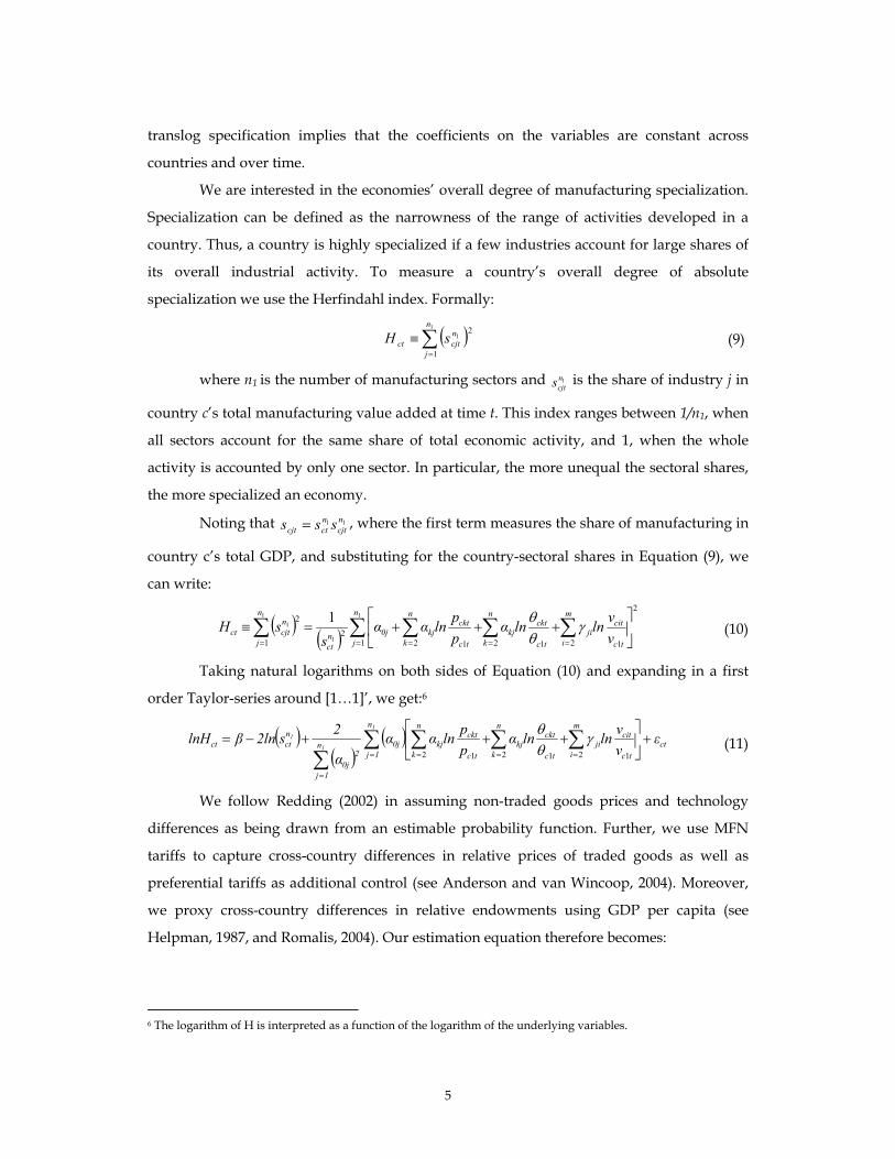
We are interested in the economies’ overall degree of manufacturing specialization.

Specialization can be defined as the narrowness of the range of activities developed in a

country. Thus, a country is highly specialized if a few industries account for large shares of

its overall industrial activity. To measure a country’s overall degree of absolute

specialization we use the Herfindahl index. Formally:

( )∑=

≡1

1

1

2n

j

ncjtct sH (9)

where n1 is the number of manufacturing sectors and 1ncjts is the share of industry j in

country c’s total manufacturing value added at time t. This index ranges between 1/n1, when

all sectors account for the same share of total economic activity, and 1, when the whole

activity is accounted by only one sector. In particular, the more unequal the sectoral shares,

the more specialized an economy.

Noting that 11 ncjt

nctcjt sss = , where the first term measures the share of manufacturing in

country c’s total GDP, and substituting for the country-sectoral shares in Equation (9), we

can write:

( ) ( )2

1 2 12 12 12

1

2 1

1

11

1 ∑ ∑∑∑∑= ====

+++=≡

n

j

m

i tc

citji

n

k tc

cktkj

n

k tc

cktkj0jn

ct

n

j

ncjtct v

vlnlnαpplnαα

ssH γ

θθ

(10)

Taking natural logarithms on both sides of Equation (10) and expanding in a first

order Taylor-series around [1…1]’, we get:6

( )( )

( ) ct

n

1j

m

i tc

citji

n

k tc

cktkj

n

k tc

cktkj0jn

1j

20j

nctct ε

vvlnlnα

pplnαα

α

2s2lnβlnH1

1

1 +

+++−= ∑ ∑∑∑

∑ = ===

=

2 12 12 1

γθθ

(11)

We follow Redding (2002) in assuming non-traded goods prices and technology

differences as being drawn from an estimable probability function. Further, we use MFN

tariffs to capture cross-country differences in relative prices of traded goods as well as

preferential tariffs as additional control (see Anderson and van Wincoop, 2004). Moreover,

we proxy cross-country differences in relative endowments using GDP per capita (see

Helpman, 1987, and Romalis, 2004). Our estimation equation therefore becomes:

6 The logarithm of H is interpreted as a function of the logarithm of the underlying variables.

6

( ) ( ) ( )[ ] cttcct3Pct

MFNct2

MFNct1ct ερηlnGDPPCδτ1τ1lnδτ1lnδlnH +++++−+++= ln (12)

where MFNctτ is the average MFN tariff set by country c at time t; P

ctτ is the average

preferential tariff set by country c at time t (within the Latin American Integration

Association LAIA or in the most important sub-regional trade agreement in which the

country is member is member), so that the term in brackets is a measure of preferential

margin; ctGPDPPC is the Gross Domestic Product per Capita of country c at time t; cη are

country fixed effects that control for any permanent country-specific barriers to trade (e.g.,

remoteness), any permanent country-differences in technology (e.g., associated as social

infrastructure, see Hall and Jones, 1999) and/or any permanent country-differences in the

relative importance of manufacturing; and tρ are year fixed effects that capture common

changes in relative prices, technologies, factor endowments, and manufacturing shares

across countries.

One well known result of the standard international trade theory is that unilateral

trade liberalization induces countries to specialize according to their overall comparative

advantage. Declining external trade barriers are thus associated with a diminished range of

commodities domestically produced and an expanded range of goods import from abroad,

i.e., increased specialization. This result holds both in the Ricardian as well as in the

Heckscher-Ohlin model (see Dornbusch et al., 1977, and Romalis, 2004). We expect then the

estimated coefficient on MFN to be significantly negative, i.e., higher tariffs lead to sectoral

diversification in production and vice versa. On the other hand, regional trade integration

leads economies to specialize according to their regional comparative advantage (see

Venables, 2003). This would also imply a reduction in the range of goods produced at home.

A priori, conditional on the degree of external openness, this might further increase

specialization, i.e., stronger concentration of manufacturing activity in fewer sectors.

Furthermore, a negative estimated coefficient on GDP per capita is also expected.

This can be explained in terms of preference or portfolio arguments. In the presence of non-

homothetic preferences, changing consumption patterns towards greater diversity prevails

as income growth, which induces matching changes in the structure of production when

trade costs are very high (see Imbs and Wacziarg, 2003). The second reason relates to the fact

that, because of indivisibilities, sectoral diversification opportunities improve with the

aggregate capital stock and the level of development (see Acemoglu and Zilibotti, 1997).

7

The Herfindahl index is a common measure of sectoral concentration in the

international trade and economic geography literatures (see, e.g., Sapir, 1996, Haaland et al.,

1999). This is however only one measure among many different ones and, a priori, there is no

reason to favor one over the other. Therefore, to check the robustness of our results, we

follow Imbs and Wacziarg (2003) in using also the Gini coefficient based on sector shares.

This coefficient, like the previous indicator, increases with higher inequality in sectoral

shares (see Cowell, 2002).

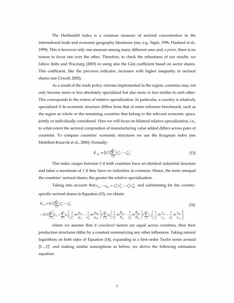
As a result of the trade policy reforms implemented in the region, countries may not

only become more or less absolutely specialized but also more or less similar to each other.

This corresponds to the notion of relative specialization. In particular, a country is relatively

specialized if its economic structure differs from that of some reference benchmark, such as

the region as whole or the remaining countries that belong to the relevant economic space,

jointly or individually considered. Here we will focus on bilateral relative specialization, i.e.,

to what extent the sectoral composition of manufacturing value added differs across pairs of

countries. To compare countries’ economic structures we use the Krugman index (see

Midelfart-Knarvik et al., 2000). Formally:

( )∑=

−≡1

11

1

21n

j

ndjt

ncjtcdt ssK (13)

This index ranges between 0 if both countries have an identical industrial structure

and takes a maximum of 1 if they have no industries in common. Hence, the more unequal

the countries’ sectoral shares, the greater the relative specialization.

Taking into account that 1111 ndjt

ndt

ncjt

nctdjtcjt ssssss −=− and substituting for the country-

specific sectoral shares in Equation (13), we obtain:

( )

( )∑ ∑∑∑

∑

= ===

=

−+

−+

−+=

−≡

1

111111

122

1 2 112 112 11

1

11111121

21

n

j

m

i td

ditndttc

citnct

ji

n

k td

dktndttc

cktnct

kj

n

k td

dktndttc

cktnct

kjcd

n

j

ndjt

ncjtcdt

vvln

svvln

sln

sln

sα

ppln

sppln

sα

ssK

γθθ

θθλ

(14)

where we assume that if considered factors are equal across countries, then their

production structures differ by a constant summarizing any other influences. Taking natural

logarithms on both sides of Equation (14), expanding in a first–order Taylor series around

[1…1]’, and making similar assumptions as before, we derive the following estimation

equation:

8

( ) ( ) ( ) cttcddtct3Pcdt2

MFNdt

MFNct1cdt νψµlnGDPPClnGDPPCτ1lnτ1lnτ1lnlnK +++−++++−+= ϕϕϕ (15)

where we use differences in MFN tariffs and the average bilateral (preferential)

tariffs to measure differences in relative prices and differences in GDP per capita to account

for differences in relative endowments. The country-pair effects cdµ control for any

permanent country-pair specific differences in trade barriers (e.g., bilateral distances)

and/or any permanent differences in technology (e.g., originated in distinct institutional

settings), while the time fixed effects tψ capture common changes across countries in

relative prices, technology, and factor endowments.

Given that Latin American countries have comparative advantage in a relatively

homogenous subset of industries with respect to the rest of the world, our hypothesis is that

the sign of the estimated coefficient on the first term (i.e., bilateral differences in MFN tariffs)

will be positive, i.e., larger differences in MFN tariffs and thus in the nominal average

protection conceded to domestic production will result in increased divergence of industrial

structures. On the other hand, the impact of bilateral tariff barriers on the degree of sectoral

dissimilarity of manufacturing production will be negative, i.e., for given extra-zone trade

impediments, bilateral (preferential) trade liberalization will induce inter-industry

specialization so that countries’ economic structure will tend to be more dissimilar. Under

the relative tariff structure associated with a preferential trade arrangement, some

commodities that were originally domestically produced become to be imported from those

partners that, even with a comparative disadvantage relative to the rest of the world, have a

regional comparative advantage, so that sectoral composition of countries’ production may

be expected to diverge. We are of course aware that opening may favor intra-industry

specialization (see Frankel and Rose, 1998). However, as discussed in Venables (2003), we

believe that the first case is more likely among developing countries like the ones we are

considering here. Finally, we expect the difference in the relative endowments and levels of

development (i.e., differences in GDPPC) to be positive.

3.2 Econometric Issues

In estimating Equations (12) and (15), there are several econometric issues that must be

addressed. First, our raw dependent variables, the absolute specialization index H and the

relative specialization index K, can only adopt values within [0,1] so that they are truncated.

As a consequence, classical estimation will lead to biased estimates. Their natural logarithms

9

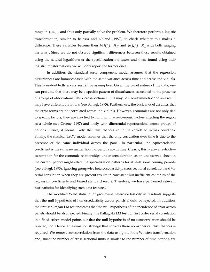
range in )0,(−∞ and thus only partially solve the problem. We therefore perform a logistic

transformation, similar to Balassa and Noland (1989), to check whether this makes a

difference. These variables become then ( )( )H1Hln − and ( )( )K1Kln − with both ranging

in ),( +∞−∞ . Since we do not observe significant differences between those results obtained

using the natural logarithms of the specialization indicators and those found using their

logistic transformations, we will only report the former ones.

In addition, the standard error component model assumes that the regression

disturbances are homoscedastic with the same variance across time and across individuals.

This is undoubtedly a very restrictive assumption. Given the panel nature of the data, one

can presume that there may be a specific pattern of disturbances associated to the presence

of groups of observations. Thus, cross-sectional units may be size-asymmetric and as a result

may have different variations (see Baltagi, 1995). Furthermore, the basic model assumes that

the error terms are not correlated across individuals. However, economies are not only tied

to specific factors, they are also tied to common macroeconomic factors affecting the region

as a whole (see Greene, 1997) and likely with differential repercussions across groups of

nations. Hence, it seems likely that disturbances could be correlated across countries.

Finally, the classical LSDV model assumes that the only correlation over time is due to the

presence of the same individual across the panel. In particular, the equicorrelation

coefficient is the same no matter how far periods are in time. Clearly, this is also a restrictive

assumption for the economic relationships under consideration, as an unobserved shock in

the current period might affect the specialization patterns for at least some coming periods

(see Baltagi, 1995). Ignoring groupwise heteroscedasticity, cross sectional correlation and/or

serial correlation when they are present results in consistent but inefficient estimates of the

regression coefficients and biased standard errors. Therefore, we have performed relevant

test statistics for identifying such data features.

The modified Wald statistic for groupwise heteroscedasticity in residuals suggests

that the null hypothesis of homoscedasticity across panels should be rejected. In addition,

the Breusch-Pagan LM test indicates that the null hypothesis of independence of error across

panels should be also rejected. Finally, the Baltagi-Li LM test for first order serial correlation

in a fixed effects model points out that the null hypothesis of no autocorrelation should be

rejected, too. Hence, an estimation strategy that corrects these non-spherical disturbances is

required. We remove autocorrelation from the data using the Prais-Winsten transformation

and, since the number of cross sectional units is similar to the number of time periods, we

10

then apply LS but replacing LS standard errors with panel-corrected standard errors

accounting for heteroscedasticity and contemporaneous correlation across panels as

indicated in Beck and Katz (1996).

Furthermore, estimating Equations (12) and (15) without controlling for relevant

additional time-varying factors, may result in biased estimates (see Greene, 1997). First, Imbs

and Wacziarg (2003) have uncovered a non-monotonic pattern of sectoral concentration of

economic activity across the development path. More specifically, higher levels of GDP per

capita are associated with lower degrees of absolute specialization up to a certain point and

increased specialization thereafter. According to Imbs and Wacziarg (2003), this relationship

might emerge as a result of different forces prevailing along the development process: forces

pushing for diversification, namely, non-homothetic preferences on the consumption side

and portfolio arguments on the investment side, and forces favoring specialization, namely,

declining trade barriers as in the Ricardian model and spatial concentration of economic

activities with increasing returns to scale as highlighted by new economic geography models

(see, e.g., Fujita et al., 1999, and Baldwin et al., 2003). We therefore include a squared GDP

per capita term to account for this non-linear relationship in Equation (12) to avoid a likely

omitted variable bias. We expect the estimated coefficients on GDPPC and GDPPC squared

to be negative and positive, respectively.

Another possible source of omitted variable biases are the episodes of real exchange

rate misalignment and, in particular, real appreciation that have been observed in Latin

America as countries implemented macroeconomic stabilization programs during the

sample period (see Edwards, 1994). In order to control for the influence of those phenomena

on the real economy, we add an index of effective exchange rate for imports or a measure of

the level of real exchange rate misalignment to Equation (12). A low and particularly an

overvalued real exchange rate (i.e., below the equilibrium level) favors imports over

domestic production and thus may induce a concentration of economic activity in sectors in

which the country has significant comparative advantage, i.e., greater production

specialization. We are also aware that this effect may be stronger, the lower the trade

barriers. An interaction between the average MFN tariffs and the real exchange rate

variables will be therefore also considered. On the other hand, a low/overvalued real

exchange rate may facilitate the imports of required inputs (capital goods) by firms in a

broader set of sectors that might become internationally competitive producers and thus

11

may foster sectoral diversification.7 The impact of real exchange rate on absolute production

specialization is then an empirical question. We also control for the effect of the exchange

rate behavior when examining relative specialization. In particular, we introduce the

absolute difference of the aforementioned measures of real exchange rate in Equation (15).

These are expected to have a positive impact on the degree of difference of countries’

manufacturing structures.

Finally, some endogeneity problems may be involved. Tariffs, both MFN and

preferential, may endogenous. Thus, protectionism could be expected to be fiercer in larger,

more diversified economies, since trade liberalization would affect many sectors and larger

shares of population. On the other hand, smaller, less diversified economies have

traditionally received special treatment in Latin America. These countries have conceded

smaller tariff preferences to larger neighbors at least for certain periods. In addition, GDPPC

as well as the real exchange rate variables may be endogenous. In particular, we can think of

a simultaneity bias. Endogenous growth models highlight that an economy’s pattern of

international specialization and its rate of economic growth are jointly and endogenously

determined (see, e.g., Redding, 1999). The same is also true for the real exchange rate and

countries’ specialization patterns (see, e.g., Obstfeld and Rogoff, 1996). Moreover, highly

specialized countries are more prone to suffer from idiosyncratic business cycles and thus

from higher expected exchange rate variability and larger average misalignments.

In order to check the robustness of our results we have therefore carried out GMM

estimations and performed the Sargan and Hansen tests for overidentifying restrictions. In

particular, two main dynamic panel estimators can be considered: those proposed by

Arellano and Bond (1991) (“Differenced GMM”) and Blundell and Bond (1998) (“System

GMM”). It is well known that for short panels with a large number of cross sectional units

highly persistent series lead to severe finite sample bias in the first case, because the lagged

levels are weak instruments of the differences. This is not the case for our econometric

analysis of absolute manufacturing specialization. The number of time periods (14 years) is

larger than the number of panels (10 countries) and, even though there is evidence of

persistence, this not strong enough to be a cause of concern.8 We will therefore only report

7 Rebelo and Vegh (1995) maintain that exchange rate-based stabilizations have tended to be associated with real exchange rate appreciations and sharp deterioration of external accounts reflecting a large increase of durables and capital goods imports. 8 The estimated rho parameter is around 0.400. The estimated coefficient on the lagged dependent variable according to the bias-corrected LSDV estimator developed by Kiviet (1995) is around 0.600. Further, we find that

12

estimates based on the method proposed by Arellano and Bond (1991). In contrast, the data

used to perform estimations on relative specialization requires a more careful investigation,

as the number of cross-sectional units, i.e., country pairs (45), is significantly larger than the

number of years (14). Further, the number of observations is relatively large (around 500),

which allows using a richer set of instruments. Hence, we will also present results obtained

according to the method developed by Blundell and Bond (1998).

4 Trade Policy Reforms in Latin America

During more than 40 years most Latin American countries maintained high tariff barriers

with the rest of the world to support a strategy of import-substituting industrialization.

Since the mid-1980s these countries started to implement trade policy reforms consisting of

sharp cuts of nominal tariffs, reduction of tariff dispersion, and elimination of non-tariff

barriers. The pace of these reforms was particularly rapid during the second half of the 1980s

and the early 1990s. Thus, simple average MFN tariff in our sample countries fell almost 30

percentage points from 41.57% in 1985 to 13.09% in 2001 with most of this drop taking place

between 1985 and 1992. Figure 1 presents the evolution of average MFN tariffs per country

over the sample period. Note that in most countries tariffs reached a peak before they begun

to be reduced as they were increased in anticipation of the future diminutions to delay

effective liberalization and thus smooth the consequent adjustment. At the initial year we

can identify three groups of countries with tariffs higher than 50% (Brazil, Colombia,

Ecuador, and Peru), countries with intermediate tariffs (Argentina, Mexico, Uruguay, and

Venezuela), and countries with average tariffs around and below 20% (Bolivia, Chile, and

Paraguay). By 1992, after drastic slashes with varying intensity across countries, the

dispersion of MFN tariff in the region had fallen from 17.25 in 1985 to 3.48.

Countries under examination have also opened their economies on a preferential

basis. LAIA is an area of economic preferences created in 1980 trough the Montevideo

Treaty. In virtue of this arrangement, countries conceded tariff preferences with respect to

the rest of the world either to all remaining member nations or to a certain subset of them.

Thus, tariffs within the region have been lower than MFN tariffs and have been reduced

even more dramatically. The average preferential tariff faced by countries being analyzed

this coefficient is almost identical when estimating pure autoregressive models using both the Arellano and Bond (1991) and Blundel and Bond (1998) estimators (0.373 and 0.400, respectively).

13

fell from 39.91% in 1985 to 5.98% in 2001. Figure 2 highlights the evolution of average

preferential tariffs set by each county in our sample. Notice that these tariffs experienced a

substantial drop during the early 1990s.

The asymmetric path of MFN and preferential tariffs implied an important increase

in the average preferential margin, which reached 111.61% in 2001 after beginning with

4.31% in 1985. This regional dimension of trade liberalization was additionally deepened by

preferential integration agreements formed by subsets of the countries. The most important

initiatives for our sample countries are MERCOSUR, which was established in 1991 by

Argentina, Brazil, Paraguay, and Uruguay, and the Andean Community, a trading

arrangement formed by Bolivia, Colombia, Ecuador, Peru, and Venezuela. In 2001 average

intra-zone tariffs within these blocs ranged between 2% and 3%.

5 The Impact of Trade Policy Reforms on Manufacturing Specialization Patterns

5.1 Trade Policy Reforms and Absolute Manufacturing Production Specialization

Figure 3 plots the trend of the Herfindahl specialization index based on sectoral value added

shares for each country in the sample over the period 1985-1998. In general, as expected, the

larger countries, Argentina, Brazil, and Mexico, exhibit lower levels of absolute

manufacturing specialization. Most Latin American countries are specialized in exploiting

their natural resources endowments. The share of food products ranges between 0.10 and

0.25 with the highest relative importance in the industrial structures of Southern Cone

countries. In addition, petroleum refineries account for large shares of total manufacturing

activity in Argentina, Bolivia, Ecuador, Uruguay, and Venezuela.

Specialization seems to follow an upward trend in most countries. In fact, regressing

the Herfindahl Index on a time trend, we find that six out of ten countries experienced

significant increases in their overall levels of production specialization: Brazil, Colombia

(from 1987 onwards), Ecuador, Peru, Uruguay, and Venezuela.9 This essentially reflects

developments in the countries’ larger manufacturing sectors. For example, in Ecuador the

combined share of the two largest industries, food products and petroleum refineries, grew

9 We have tested for non-stationarity to determine whether there are concrete reasons to be concerned about this issue. In particular, we have performed the Levin-Lin-Chu test (Levin et al., 2002) for panel unit roots on the specialization variable for alternative balanced panels. In doing this, we have introduced one lag of this variable to allow for serial correlation in the errors. The null hypothesis of unit root is strongly rejected for all considered configurations, regardless whether we include a time trend or not.

14

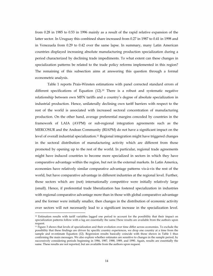
from 0.28 in 1985 to 0.53 in 1996 mainly as a result of the rapid relative expansion of the

latter sector. In Uruguay this combined share increased from 0.27 in 1987 to 0.41 in 1998 and

in Venezuela from 0.29 to 0.42 over the same lapse. In summary, many Latin American

countries displayed increasing absolute manufacturing production specialization during a

period characterized by declining trade impediments. To what extent can these changes in

specialization patterns be related to the trade policy reforms implemented in this region?

The remaining of this subsection aims at answering this question through a formal

econometric analysis.

Table 1 reports Prais-Winsten estimations with panel corrected standard errors of

different specifications of Equation (12).10 There is a robust and systematic negative

relationship between own MFN tariffs and a country’s degree of absolute specialization in

industrial production. Hence, unilaterally declining own tariff barriers with respect to the

rest of the world is associated with increased sectoral concentration of manufacturing

production. On the other hand, average preferential margins conceded by countries in the

framework of LAIA (AVPM) or sub-regional integration agreements such as the

MERCOSUR and the Andean Community (RIAPM) do not have a significant impact on the

level of overall industrial specialization.11 Regional integration might have triggered changes

in the sectoral distribution of manufacturing activity which are different from those

promoted by opening up to the rest of the world. In particular, regional trade agreements

might have induced countries to become more specialized in sectors in which they have

comparative advantage within the region, but not in the external markets. In Latin America,

economies have relatively similar comparative advantage patterns vis-à-vis the rest of the

world, but have comparative advantage in different industries at the regional level. Further,

those sectors which are (not) internationally competitive were initially relatively large

(small). Hence, if preferential trade liberalization has fostered specialization in industries

with regional comparative advantage more than in those with global comparative advantage

and the former were initially smaller, then changes in the distribution of economic activity

over sectors will not necessarily lead to a significant increase in the specialization level. 10 Estimation results with tariff variables lagged one period to account for the possibility that their impact on specialization patterns follow with a lag are essentially the same.These results are available from the authors upon request. 11 Figure 3 shows that levels of specialization and their evolution over time differ across economies. To exclude the possibility that these findings are driven by specific country experiences, we drop one country at a time from the sample and re-estimate Equation (12). Regression results basically coincide with those shown in Table 1 thus confirming the main messages. We also explore whether estimates are sensitive to changes in the sample period, by successively considering periods beginning in 1986, 1987, 1988, 1989, and 1990. Again, results are essentially the same. These results are not reported, but are available from the authors upon request.

15

Then, depending on the initial industrial structure, the impact on overall specialization

might be weaker in this case.

Previous estimations control for country specific factors that remain constants over

time as well as common changes across countries. However, according to economic theory,

there are important additional time-varying country-specific factors that may affect the

degree of industrial specialization and thus the relation under examination. One of these

factors is relative endowment as proxied by the GDP per capita. Results including these

variables are presented in Columns 4 and 5 of Table 1. As expected, the estimated coefficient

on GDPPC is negative and significant, while that on the squared GDPPC is positive and

significant across the different specifications. Hence, there is non-linear (U-shaped)

relationship between sectoral concentration of manufacturing value added and the level of

per capital income, i.e., first sectoral diversification occurs, but there is a level of per capital

income beyond which countries start to specialize again. This coincides with findings

reported in Imbs and Wacziarg (2003).

Another important time-varying factor whose omission may lead to biases estimates

is the real exchange rate. Estimates obtained when incorporating this variable are shown in

Table 2. Without considering potential nonlinearities, the real effective exchange rate for

imports seems to be positively related to the overall level of specialization (Column 1).

However, when its interplay with trade policy is accounted for, the estimated coefficient on

this exchange rate variable is negative and significant, whereas that on the interaction term

is positive and significant (Column 2). Thus, we observe that the higher MFN tariffs and real

exchange rate, the greater the absolute manufacturing specialization. In the case of real

exchange rate misalignment, the same sign pattern prevail, but estimated coefficients are not

significantly different from zero (Column 4). Henceforth, there is some evidence suggesting

that a high exchange rate induces manufacturing production diversification when trade

barriers are low, but promote industrial specialization when coupled with high tariff

barriers.

We check the robustness of our results to the specialization measure being used and

the econometric strategy. We first replicate previous regressions using the logarithm of the

Gini coefficient calculated on sectoral manufacturing value added instead of the Herfindahl

index as dependent variable. Estimations are reported in Tables 3 and 4 and they confirm

most of our previous findings. Table 5 presents results obtained performing GMM

estimations using the procedure proposed by Arellano and Bond (1991). These estimations

16

aim at addressing possible endogeneity problems in the regressions discusses above. Our

main conclusion still holds. Unilateral trade liberalization, i.e., reducing own MFN tariffs

with respect to the rest of the world is associated with more concentrated manufacturing

production structures. Estimated coefficients on remaining variables are similar to those

reported in Table 2, except the one on the interaction between real exchange rate

misalignment and tariffs, which now becomes significantly positive thus providing

additional evidence of non-monotonicities in the impact of exchange rate on overall absolute

specialization.12

This sub-section has revealed that trade policy reforms in Latin America have had a

substantial impact on countries’ international specialization patterns. In particular, unilateral

opening has favored increasing manufacturing production specialization. Trade

liberalization initiatives may also influence relative specialization across country pairs. More

specifically, the magnitude of the differences in the extent to which nations liberalize their

trade flows with the rest of the world as well as the level of bilateral (preferential) trade

barriers may affect how similar is the sectoral composition of manufacturing production

across country pairs. The following sub-section assesses this possibility.

5.2 Trade Policy Reforms and Manufacturing Production Structures: Convergence or

Divergence?

We measure relative manufacturing specialization with the Krugman index. This

index quantifies the degree of bilateral sectoral disparity of industrial structures. Figure 4

presents the Krugman index for each country pair in our sample over the period 1985-1998.

According to a simple regression of this index on a time trend, 22 out of 45 country pairs

became more dissimilar in terms of their manufacturing structures and 7 out of 45 do not

exhibit significant changes.13 Interestingly, half of the 16 cases of reductions involve Bolivia,

12 There is an additional, more complicated issue in this analysis, namely, if specialization, tariffs, and the level of development are jointly determined, there will be both direct and indirect effects that should be disentangled. For example, real exchange rate misaligments may have direct effects on specialization as well as indirect effects through the influence that they likely exert on choosing the level of tariff protection. We have therefore estimated alternative specifications of systems of equations by 3SLS and GMM where these variables are simultaneously treated as endogenous. This multiple equation strategy generates similar results to those from the single equation one. In addition, we observe that less diversified economies indeed set lower tariffs and tend to have lower levels of GDP per capita. These results are not reported but are available from the authors upon request. 13 We have tested for non-stationarity of the specialization measure also in thie case. The Levin-Lin-Chu test (Levin et al., 2002) for panel unit roots suggests that series are stattionary. This holds regardless whether we include a time trend or not and the specific balanced panel being considered.

17

which moved towards convergence in terms of sectoral distribution of economic activity

after starting as the most dissimilar nation for each of its Latin American partners.14

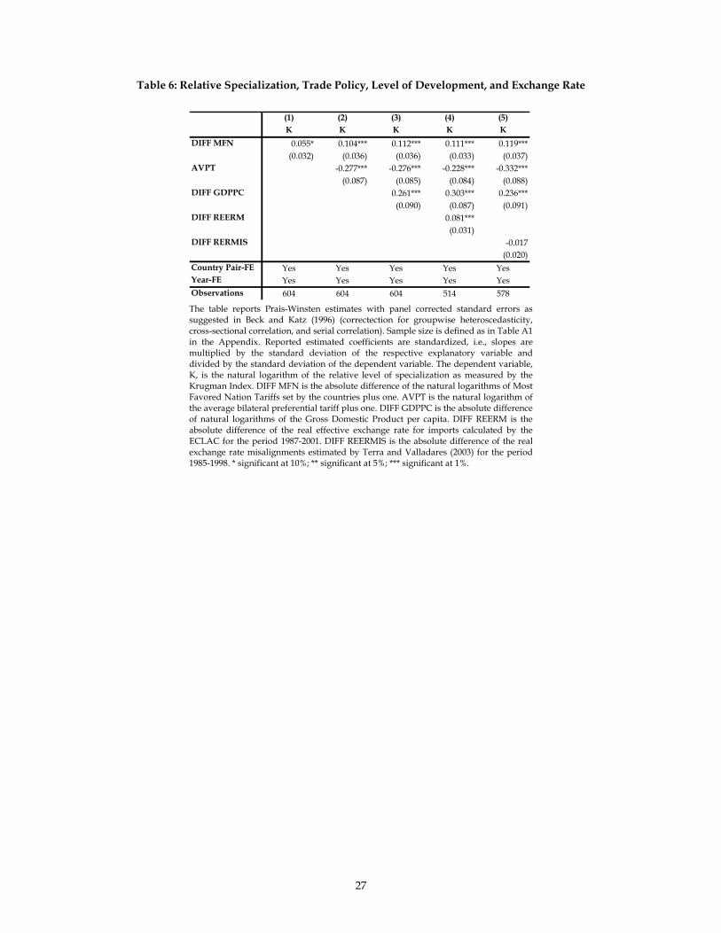
Table 6 presents Prais-Winsten estimations with panel corrected standard errors of

Equation (14). Two main results outstand. As expected, larger differences in the degree of

unilateral openness with respect to the rest of the world and deeper bilateral (preferential)

trade liberalization foster a higher degree of relative specialization, i.e., more dissimilar

industrial structures. This is consistently true from the basic specification also when the level

of development and variable reflecting the level of real exchange rate are introduced. In this

sense, we should mention that larger differences in the real effective exchange rate for

imports are associated with larger disparities in the sectoral distribution of manufacturing

production.

Table 7 shows that the core findings are confirmed after implementing GMM

procedures to correct endogeneity biases: the Arellano and Bond (1991) estimator and the

Blundell and Bond (1998) estimator. Two considerations deserve being made. First, while

differences in the real exchange rate for imports seem to be an important factor influencing

cross-country differences in manufacturing structures according to the former estimator,

differences in the degree of real exchange rate misalignment is the relevant one when the

latter estimator is used. Second, although both sets of estimates are consistent as suggested

by the respective specification tests, these distinct results across methods recommend to

perform a carefully comparison. As mentioned before, highly persistent series may generate

weak instrument problems and thus serious finite sample biases when applying the

Arellano and Bond estimator. This may be detected by comparing the estimated coefficient

on the lagged dependent variable to those from OLS, which is upward biased, and LSDV

(Within), which is downward biased (see Bond, 2002). In our case, these coefficients are

0.854 and 0.497, respectively, for the model specification shown in Columns 2 and 5.

Estimates reported in Table 7 indicate that there is indeed evidence that the Arellano and

Bond estimator is affected by finite sample bias. In contrast, the Blundel and Bond estimator

produces an estimate which is well below the OLS one and well above the LSDV one thus

appearing as our preferred estimation strategy.

Hence, regional trade integration seems to have spurred inter-industry

specialization across countries. This has profound macroeconomic implications. If countries

14 Bolivia is one the poorest country in the region and suffered from a severe hyperinflation episode during the first part of the 1980s.

18

become more dissimilar in terms of their production structures and thus more sensitive to

specific industry shocks, more idiosyncratic business cycles would prevail (see Kenen, 1969,

Eichengreen, 1992, and Krugman, 1993) and, if exchange rates are used as an adjustment

mechanism to dampen cyclical fluctuations, higher bilateral exchange rate variability should

be expected. This, in turn, might act as channel of agglomeration of economic activities in

the larger countries in the region (see Ricci, 1998) and might promote reversions in the

integration process in the form of reinsertion of protectionist measures (see Eichengreen,

1993, and Fernández-Arias et al., 2002).

6 Concluding Remarks

This paper has aimed at answering one main question: Did Latin American countries

become more and differently specialized as a consequence of trade policy reforms? Our

econometric analysis shows that the answer is yes.

Unilateral trade liberalization has resulted in increased absolute manufacturing

production specialization. Weinhold and Rauch (1999) show that, at least for developing

countries, this might have a positive impact, since specialization appears to be positively

and significantly correlated with manufacturing productivity growth. One possible

explanation for this result comes from models with endogenous growth through learning-

by-doing. In this framework, increased openness to international trade can lead to increased

specialization, which in turn accelerates productivity growth by more fully realizing

dynamic economies of scale. Of course, not only the degree, but also the nature of

specialization is important (see Redding, 1999, and Bensidoun et al., 2001). In Latin America,

industrial activity has on average become increasingly concentrated in sectors using

intensively natural resources endowments. What does this imply for this region? According

to Perri et al. (2001), the experience of other countries such as Australia, Canada, Sweden

and Finland show that these rich endowments, when properly combined with policies

stimulating the adoption of new technologies, are a proven growth recipe.

Preferential trade liberalization has favored a broadening of the disparities between

countries’ economic structures. This has important implications for the regional

macroeconomics and the sustainability of ongoing integration processes. Inter-industry

specialization and thus higher sensitivity to industry specific shocks are associated with

more idiosyncratic business cycles and higher expected exchange rate variability, which in

19

turn affect locational incentives and trade flows generating pressures for reintroducing

protectionist measures.

The previous findings seem to be quite robust. They hold regardless the

specialization measure being used, the inclusion of control variables such the real effective

exchange rate for imports and the real exchange rate misalignment, and remain valid after

using GMM procedures to correct biases originated in serial correlation and endogeneity.

20

Figure 1

Figure 2

0.2

.4.6

.80

.2.4

.6.8

0.2

.4.6

.8

1985 1990 1995 2000 1985 1990 1995 2000

1985 1990 1995 2000 1985 1990 1995 2000

Argentina Bolivia Brazil Chile

Colombia Ecuador Mexico Peru

Uruguay Venezuela

Mos

t Fav

ored

Nat

ion

Tarif

f

.

.

0.2

.4.6

.80

.2.4

.6.8

0.2

.4.6

.8

1985 1990 1995 2000 1985 1990 1995 2000

1985 1990 1995 2000 1985 1990 1995 2000

Argentina Bolivia Brazil Chile

Colombia Ecuador Mexico Peru

Uruguay Venezuela

Pref

eren

tial T

ariff

.

.

21

Figure 3

The figure shows the trend of the Herfindahl Index for each of the sample countries as obtained using the filter proposed by Hodrick and Prescott (1997).

Figure 4

The figure shows the trend of the Krugman Index for each of the sample country pairs as obtained using the filter proposed by Hodrick and Prescott (1997).

.08

.081

.082

.083

.084

.2.2

5.3

.06

.065

.07

.085

.09

.095

.1.1

05

.075

.08

.085

.09

.1.1

5.2

.071

5.0

72.0

725

.073

.073

5

.07

.075

.08

.085

.08

.09

.1.1

1

.08

.1.1

2.1

4

1985 1990 1995 2000 1985 1990 1995 2000

1985 1990 1995 2000 1985 1990 1995 2000

Argentina Bolivia Brazil Chile

Colombia Ecuador Mexico Peru

Uruguay Venezuela

Abs

olut

e Sp

ecia

lizat

ion

- Her

finda

hl In

dex

.

.

.85

.9.9

5

.44.4

5.46

.47.

48

.6.6

1.62

.63.

64

.47

.48.

49.5

.51

.5.6

.7.8

.385

.39.3

95.4

.405

.5.5

5.6

.65

.7

.4.4

5.5

.55

.6

.35

.4.4

5.5

.55

1.11

.121.

141.1

61.18

.8.9

11.

1

.85

.9.9

51

.4.6

.81

11.

021.

041.

06

.7.7

5.8

.85

.7.8

.9

.6.7

.8.9

1

.65

.7.7

5

.5.5

5.6

.7.8

.91

.38

.39

.4.4

1

.6.7

.8

.65

.7.7

5.8

.55

.6.6

5.7

.75

.45

.5.5

5.6

.65

.6.7

.8.9

.56

.58

.6.6

2

.55

.6.6

5.7

.55

.6.6

5.7

.6.6

5.7

.75

.4.5

.6.7

.8

.3.3

5.4

.45

.5.5

5.6

.65

.4.4

5.5

.6.6

5.7

.75

.4.6

.81

.6.6

5.7

.75

.55

.6.6

5.7

.75

.5.6

.7.8

.45

.5.5

5.6

.65

.5.6

.7.8

.55

.6.6

5.7

.75

.5.5

5.6

.65

.6.7

.8

.5.6

.7.8

1985 1990 1995 2000 1985 1990 1995 2000 1985 1990 1995 2000 1985 1990 1995 2000

1985 1990 1995 2000 1985 1990 1995 2000 1985 1990 1995 2000

Argentina-Bolivia Argentina-Brazil Argentina-Chile Argentina-Colombia Argentina-Ecuador Argentina-Mexico Argentina-Peru

Argentina-Uruguay Argentina-Venezuela Bolivia-Brazil Bolivia-Chile Bolivia-Colombia Bolivia-Ecuador Bolivia-Mexico

Bolivia-Peru Bolivia-Uruguay Bolivia-Venezuela Brazil-Chile Brazil-Colombia Brazil-Ecuador Brazil-Mexico

Brazil-Peru Brazil-Uruguay Brazil-Venezuela Chile-Colombia Chile-Ecuador Chile-Mexico Chile-Peru

Chile-Uruguay Chile-Venezuela Colombia-Ecuador Colombia-Mexico Colombia-Peru Colombia-Uruguay Colombia-Venezuela

Ecuador-Mexico Ecuador-Peru Ecuador-Uruguay Ecuador-Venezuela Mexico-Peru Mexico-Uruguay Mexico-Venezuela

Peru-Uruguay Peru-Venezuela Uruguay-Venezuela

Rela

tive

Spec

ializ

atio

n - K

rugm

an In

dex

.

.

22

Table 1: The Impact of Unilateral and Preferential Trade Policy on Absolute Specialization

The table reports Prais-Winsten estimates with panel corrected standard errors as suggested in Beck and Katz (1996) (correctection for groupwise heteroscedasticity, cross-sectional correlation, and serial correlation). Reported estimated coefficients are standardized, i.e., slopes are multiplied by the standard deviation of the respective explanatory variable and divided by the standard deviation of the dependent variable. Sample size is defined as in Table A1 in the Appendix. The dependent variable, H, is the natural logarithm of the overall level of specialization as measured by the Herfindahl Index. MFN is the natural logarithm of the average Most Favored Nation Tariff set by the country plus one. AVPM is the average preferential margin conceded by the country to Latin American partners, i.e., the natural logarithm of MFN plus one minus the natural logarithm of AVPT plus one, where AVPT is the average preferential tariff applied on trade flows with members of the LAIA. RIAPM is the average preferential margin conceded by the country within the most important RIA with Latin American partners, i.e., the natural logarithm of MFN plus one minus the natural logarithm of RIAPT plus one, where RIAPT is the average preferential tariff applied on trade flows with members of this agreement. GDPPC is the natural logarithm of Gross Domestic Product per capita (GDPPC2: squared). * significant at 10%; ** significant at 5%; *** significant at 1%.

(1) (2) (3) (4) (5)H H H H H

MFN -0.245*** -0.308*** -0.301*** -0.228*** -0.220***(0.061) (0.080) (0.068) (0.077) (0.075)

AVPM 0.098(0.077)

RIAPM 0.124 0.096 0.097(0.079) (0.079) (0.082)

GDPPC -0.559** -7.347**(0.229) (3.342)

GDPPC2 6.485**(3.238)

Country-FE Yes Yes Yes Yes YesYear-FE Yes Yes Yes Yes YesObservations 137 137 137 137 137

23

Table 2: Absolute Specialization, Trade Policy, Level of Development, and Exchange Rate

The table reports Prais-Winsten estimates with panel corrected standard errors as suggested in Beck and Katz (1996) (correctection for groupwise heteroscedasticity, cross-sectional correlation, and serial correlation). Reported estimated coefficients are standardized, i.e., slopes are multiplied by the standard deviation of the respective explanatory variable and divided by the standard deviation of the dependent variable. Sample size is defined as in Table A1 in the Appendix. The dependent variable, H, is the natural logarithm of the overall level of specialization as measured by the Herfindahl Index. MFN is the natural logarithm of the average Most Favored Nation Tariff set by the country plus one. RIAPM is the average preferential margin conceded by the country within the most important RIA with Latin American partners, i.e., the natural logarithm of MFN plus one minus the natural logarithm of RIAPT plus one, where RIAPT is the average preferential tariff applied on trade flows with members of this agreement. GDPPC is the natural logarithm of Gross Domestic Product per capita (GDPPC2: squared). REERM is the real effective exchange rate for imports calculated by the ECLAC for the period 1987-2001. REERMIS is the real exchange rate misalignment estimated by Terra and Valladares (2003) for the period 1985-1998. * significant at 10%; ** significant at 5%; *** significant at 1%.

(1) (2) (3) (4)H H H H

MFN -0.271** -0.681*** -0.213** -0.230***(0.086) (0.162) (0.083) (0.080)

RIAPM 0.169 0.121 0.032 0.028(0.106) (0.104) (0.081) (0.085)

GDPPC -9.725** -10.632*** -8.034** -8.767**(4.120) (3.810) (3.626) (3.500)

GDPPC2 8.825** 9.485*** 7.190** 7.835**(3.866) (3.552) (3.422) (3.294)

REERM 0.062* -0.148*(0.038) (0.077)

RERMIS 0.055* -0.054(0.033) (0.074)

MFN x REERM 0.005***(0.002)

MFN x RERMIS 0.111(0.070)

Country-FE Yes Yes Yes YesYear-FE Yes Yes Yes YesObservations 117 117 134 134

24

Table 3: The Impact of Unilateral and Preferential Trade Policy on Absolute Specialization (Alternative Specialization Measure)

The table reports Prais-Winsten estimates with panel corrected standard errors as suggested in Beck and Katz (1996) (correctection for groupwise heteroscedasticity, cross-sectional correlation, and serial correlation). Reported estimated coefficients are standardized, i.e., slopes are multiplied by the standard deviation of the respective explanatory variable and divided by the standard deviation of the dependent variable. Sample size is defined as in Table A1 in the Appendix. The dependent variable, G, is the natural logarithm of the overall level of specialization as measured by the Gini Coefficient. MFN is the natural logarithm of the average Most Favored Nation Tariff set by the country plus one. RIAPM is the average preferential margin conceded by the country within the most important RIA with Latin American partners, i.e., the natural logarithm of MFN plus one minus the natural logarithm of RIAPT plus one, where RIAPT is the average preferential tariff applied on trade flows with members of this agreement. GDPPC is the natural logarithm of Gross Domestic Product per capita (GDPPC2: squared). * significant at 10%; ** significant at 5%; *** significant at 1%.

(1) (2) (3) (4) (5)G G G G G

MFN -0.207*** -0.283*** -0.261*** -0.144** -0.138**(0.056) (0.073) (0.064) (0.065) (0.063)

AVPM 0.120*(0.070)

RIAPM 0.120* 0.076 0.074(0.073) (0.070) (0.072)

GDPPC -0.954*** -6.513**(0.220) (2.717)

GDPPC2 5.314**(2.524)

Country-FE Yes Yes Yes Yes YesYear-FE Yes Yes Yes Yes YesObservations 137 137 137 137 137

25

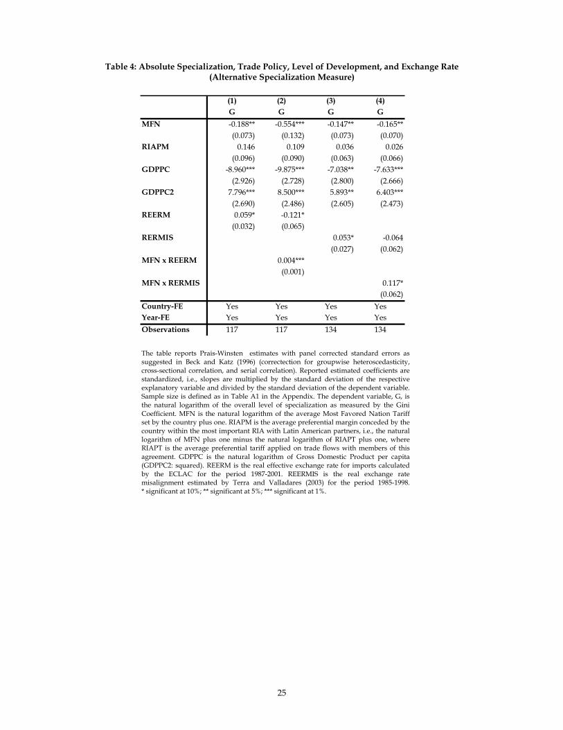
Table 4: Absolute Specialization, Trade Policy, Level of Development, and Exchange Rate (Alternative Specialization Measure)

The table reports Prais-Winsten estimates with panel corrected standard errors as suggested in Beck and Katz (1996) (correctection for groupwise heteroscedasticity, cross-sectional correlation, and serial correlation). Reported estimated coefficients are standardized, i.e., slopes are multiplied by the standard deviation of the respective explanatory variable and divided by the standard deviation of the dependent variable. Sample size is defined as in Table A1 in the Appendix. The dependent variable, G, is the natural logarithm of the overall level of specialization as measured by the Gini Coefficient. MFN is the natural logarithm of the average Most Favored Nation Tariff set by the country plus one. RIAPM is the average preferential margin conceded by the country within the most important RIA with Latin American partners, i.e., the natural logarithm of MFN plus one minus the natural logarithm of RIAPT plus one, where RIAPT is the average preferential tariff applied on trade flows with members of this agreement. GDPPC is the natural logarithm of Gross Domestic Product per capita (GDPPC2: squared). REERM is the real effective exchange rate for imports calculated by the ECLAC for the period 1987-2001. REERMIS is the real exchange rate misalignment estimated by Terra and Valladares (2003) for the period 1985-1998. * significant at 10%; ** significant at 5%; *** significant at 1%.

(1) (2) (3) (4)G G G G

MFN -0.188** -0.554*** -0.147** -0.165**(0.073) (0.132) (0.073) (0.070)

RIAPM 0.146 0.109 0.036 0.026(0.096) (0.090) (0.063) (0.066)

GDPPC -8.960*** -9.875*** -7.038** -7.633***(2.926) (2.728) (2.800) (2.666)

GDPPC2 7.796*** 8.500*** 5.893** 6.403***(2.690) (2.486) (2.605) (2.473)

REERM 0.059* -0.121*(0.032) (0.065)

RERMIS 0.053* -0.064(0.027) (0.062)

MFN x REERM 0.004***(0.001)

MFN x RERMIS 0.117*(0.062)

Country-FE Yes Yes Yes YesYear-FE Yes Yes Yes YesObservations 117 117 134 134

26

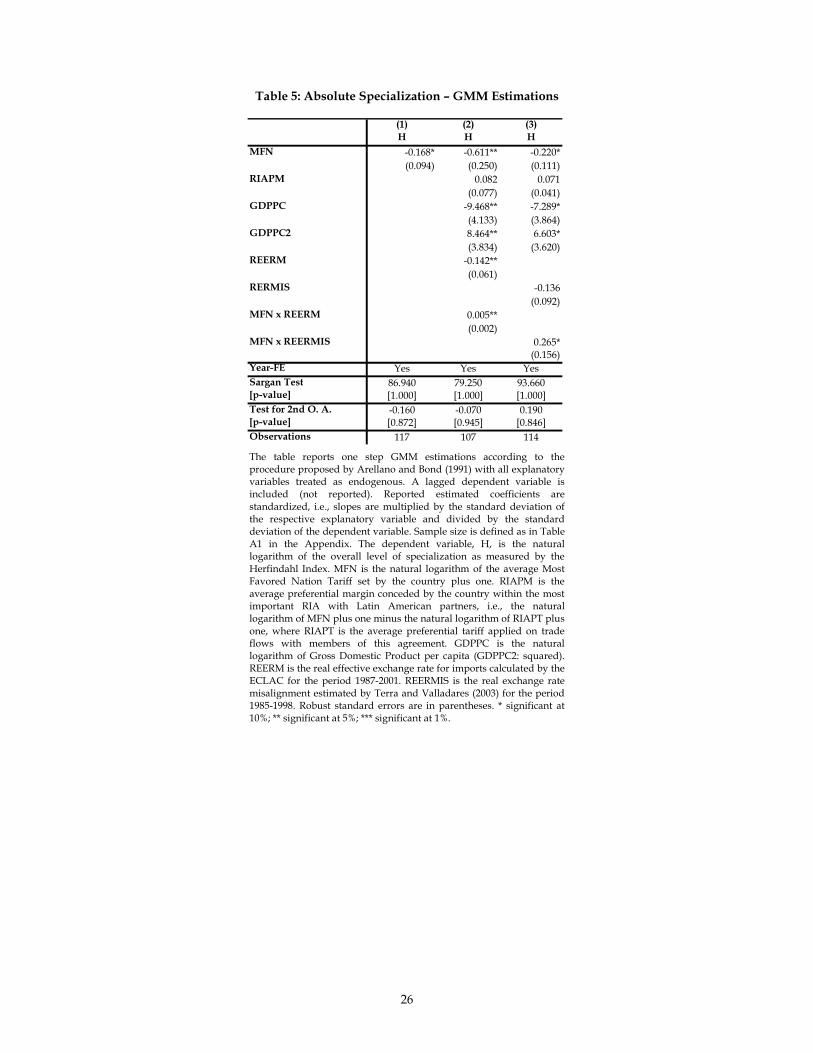
Table 5: Absolute Specialization – GMM Estimations

The table reports one step GMM estimations according to the procedure proposed by Arellano and Bond (1991) with all explanatory variables treated as endogenous. A lagged dependent variable is included (not reported). Reported estimated coefficients are standardized, i.e., slopes are multiplied by the standard deviation of the respective explanatory variable and divided by the standard deviation of the dependent variable. Sample size is defined as in Table A1 in the Appendix. The dependent variable, H, is the natural logarithm of the overall level of specialization as measured by the Herfindahl Index. MFN is the natural logarithm of the average Most Favored Nation Tariff set by the country plus one. RIAPM is the average preferential margin conceded by the country within the most important RIA with Latin American partners, i.e., the natural logarithm of MFN plus one minus the natural logarithm of RIAPT plus one, where RIAPT is the average preferential tariff applied on trade flows with members of this agreement. GDPPC is the natural logarithm of Gross Domestic Product per capita (GDPPC2: squared). REERM is the real effective exchange rate for imports calculated by the ECLAC for the period 1987-2001. REERMIS is the real exchange rate misalignment estimated by Terra and Valladares (2003) for the period 1985-1998. Robust standard errors are in parentheses. * significant at 10%; ** significant at 5%; *** significant at 1%.

(1) (2) (3)H H H

MFN -0.168* -0.611** -0.220*(0.094) (0.250) (0.111)

RIAPM 0.082 0.071(0.077) (0.041)

GDPPC -9.468** -7.289*(4.133) (3.864)

GDPPC2 8.464** 6.603*(3.834) (3.620)

REERM -0.142**(0.061)

RERMIS -0.136(0.092)

MFN x REERM 0.005**(0.002)

MFN x REERMIS 0.265*(0.156)

Year-FE Yes Yes YesSargan Test 86.940 79.250 93.660[p-value] [1.000] [1.000] [1.000]Test for 2nd O. A. -0.160 -0.070 0.190[p-value] [0.872] [0.945] [0.846]Observations 117 107 114

27

Table 6: Relative Specialization, Trade Policy, Level of Development, and Exchange Rate

The table reports Prais-Winsten estimates with panel corrected standard errors as suggested in Beck and Katz (1996) (correctection for groupwise heteroscedasticity, cross-sectional correlation, and serial correlation). Sample size is defined as in Table A1 in the Appendix. Reported estimated coefficients are standardized, i.e., slopes are multiplied by the standard deviation of the respective explanatory variable and divided by the standard deviation of the dependent variable. The dependent variable, K, is the natural logarithm of the relative level of specialization as measured by the Krugman Index. DIFF MFN is the absolute difference of the natural logarithms of Most Favored Nation Tariffs set by the countries plus one. AVPT is the natural logarithm of the average bilateral preferential tariff plus one. DIFF GDPPC is the absolute difference of natural logarithms of the Gross Domestic Product per capita. DIFF REERM is the absolute difference of the real effective exchange rate for imports calculated by the ECLAC for the period 1987-2001. DIFF REERMIS is the absolute difference of the real exchange rate misalignments estimated by Terra and Valladares (2003) for the period 1985-1998. * significant at 10%; ** significant at 5%; *** significant at 1%.

(1) (2) (3) (4) (5)K K K K K

DIFF MFN 0.055* 0.104*** 0.112*** 0.111*** 0.119***(0.032) (0.036) (0.036) (0.033) (0.037)

AVPT -0.277*** -0.276*** -0.228*** -0.332***(0.087) (0.085) (0.084) (0.088)

DIFF GDPPC 0.261*** 0.303*** 0.236***(0.090) (0.087) (0.091)

DIFF REERM 0.081***(0.031)

DIFF RERMIS -0.017(0.020)

Country Pair-FE Yes Yes Yes Yes YesYear-FE Yes Yes Yes Yes YesObservations 604 604 604 514 578

28

Table 7: Relative Specialization – GMM Estimations

Columns (1)-(3) report one-step GMM estimations according to the procedure proposed by Arellano and Bond (1991) with MFN and AVPT treated as predetermined and remaining variables as endogenous. Sample size defined as in Table A1 in the Appendix. The Sargan Test is based on two-step estimations (Arellano and Bond Estimations). Columns (4)-(6) report one-step GMM estimations according to the procedure proposed by Blundell and Bond (1998). Instrumented used are 1-5 lags of DMFN and AVPT, and 3-6 lags of DGDPPC, DRERM, DRERMIS in the level equation; and 2-6 lags of DMFN and AVPT, and 4-7 lags of DGDPPC, DRERM, DRERMIS in the difference equation. Reported estimated coefficients are standardized, i.e., slopes are multiplied by the standard deviation of the respective explanatory variable and divided by the standard deviation of the dependent variable. The dependent variable, K, is the natural logarithm of the relative level of specialization as measured by the Krugman Index (K(-1): lagged one year). DIFF MFN is the absolute difference of the natural logarithms of Most Favored Nation Tariffs set by the countries plus one. AVPT is the natural logarithm of the average bilateral preferential tariff plus one. DIFF GDPPC is the absolute difference of natural logarithms of the Gross Domestic Product per capita. DIFF REERM is the absolute difference of the real effective exchange rate for imports calculated by the ECLAC for the period 1987-2001. DIFF REERMIS is the absolute difference of the real exchange rate misalignments estimated by Terra and Valladares (2003) for the period 1985-1998. * significant at 10%; ** significant at 5%; *** significant at 1%.

(1) (2) (3) (4) (5) (6)K K K K K K

K(-1) 0.430*** 0.390*** 0.503*** 0.567*** 0.638*** 0.550***(0.066) (0.055) (0.067) (0.220) (0.192) (0.127)

DIFF MFN 0.094** 0.074 0.097** 0.139** 0.075 0.157***(0.044) (0.046) (0.040) (0.059) (0.063) (0.051)

AVPT -0.218*** -0.170** -0.237*** -0.442*** -0.285*** -0.308**(0.073) (0.069) (0.078) (0.153) (0.130) (0.146)

DIFF GDPPC 0.277 0.290* 0.297 0.241* 0.051 0.174(0.173) (0.175) (0.189) (0.146) (0.107) (0.153)

DIFF RERM 0.069** -0.125*(0.034) (0.070)

DIFF RERMIS 0.034 0.353***(0.032) (0.111)

Year-FE Yes Yes Yes Yes Yes YesSargan/Hansen Test 30.420 35.440 30.610 16.530 24.670 24.180[p-value] [1.000] [1.000] [1.000] [0.168] [0.214] [0.189]Test for 2nd O. A. -0.600 -1.050 0.570 0.910 -0.800 1.350[p-value] [0.546] [0.296] [0.571] [0.361] [0.424] [0.177]Observations 514 469 488 559 514 533

29

References

Anderson, J. and van Wincoop, E., 2004. Trade costs. Journal of Economic Literature, XLII. Acemoglu, D. and Zilibotti, F., 1997. Was Promotheus unbound by change? Risk, diversification, and

growth. Journal of Political Economy, 105, 4. Arellano, M. and Bond, S. (1991). Some tests of specification for panel data: Monte Carlo evidence and

an application to employment equations. Review of Economic Studies 58. Balassa, B. and Noland, M., 1989. The changing comparative advantage of Japan and the United

States. Journal of the Japanese and International Economics, 3. Baldwin, R., Forslid, R., Martin, P., Ottaviano, G. and Robert-Nicoud, F., 2003. Economic geography

and public policy. Princeton University Press. Baltagi, B., 1995. Econometric analysis of panel data. John Wiley & Sons. Beck, N. and Katz, J., 1996. Nuissance vs. substance: Specifying and estimating time-series-cross-

section models. Political Analysis VI. Bensidoun, I., Gaulier, G., and Ünal-Kesenci, D., 2001. The nature of specialization matters for growth:

An empirical investigation. CEPII Document de Travail 13. Blundell, R. and Bond, S., 1998. Initial conditions and moment restrictions in dynamic panel data

models. Journal of Econometrics, 87. Bond, S., 2002. Dynamic panel data models: a guide to microdata methods and practice. Portuguese

Economic Journal, 1, 2. Brülhart, M., 2001. Evolving geographical specialisation of European Manufacturing Industries.

Weltwirtschaftliches Archiv 137, 2. Combes, P. and Overman, H., 2003. The spatial distribution of economic activities in the European

Union, in Henderson, V. and Thisse, J. (eds.). Handbook of Regional and Urban Economics. Elsevier.

Cowelll, F., 2000. Measuring inequality, in Bourguignon, F. and Atkinson, A., Handbook of income distribution. North-Holland, Amsterdam.

Dixit, A. and Norman, V. The theory of international trade. Cambridge University Press, Cambridge. Dornbusch, R., Fischer, S., and Samuelson, P., 1977. Comparative advantages, trade, and payments in

a Ricardian model with a continuum of goods. American Economic Review. 67. Edwards, S., 1994. Macroeconomic stabilization in Latin America: Recent experience and some

sequencing issues. NBER Working Paper 4697. Eichengreen, B., 1992. Should the Maastricht Treaty be saved? Princeton Studies in International

Finance 74. International Finance Section, Princeton University. Eichengreen, B. 1993. European monetary unification. Journal of Economic Literature, 31. Fernández-Arias, E., Panizza, U., and Stein, E., 2002. Trade agreements, exchange rate disagreements.

Inter-American Development Bank, Washington. Frankel, J and Rose, A., 1998. The endogeneity of the optimum currency area criteria. Economic

Journal, 108, 449. Fujita, M., Krugman, P., and Venables, A., 1999. The spatial economy: Cities, regions and international

trade. MIT Press. Godlfajn, I. and Valdes, R., 1999. The aftermath of appreciations. Quarterly Journal of Economics, 114. Greene, W., 1997. Econometric Analysis. Prentice Hall, New Yersey. Haaland, J., Kind, H., Midelfart-Knarvik, K.. and Torstensson, J., 1999. What Determines the Economic

Geography of Europe? CEPR Discussion Paper 2072. Hall, R. and Jones, C., 1999. Why do some countries produce so much more output per worker than

others? Quarterly Journal of Economics, 114, 1. Harrigan, J., 1997. Technology, factor supplies, and international specialization: Estimating the

neoclassical model. American Economic Review, 87, 4. Helpman, E., 1987. Imperfect competition and international trade: Evidence from fourteen

industrialised countries. Journal of the Japanese and International Economies, 1. Hodrick, R. and Prescott, E., 1997. Postwar U.S. Business Cycles: An Empirical Investigation. Journal

of Money, Credit, and Banking, 29. Imbs, J. and Wacziarg, R., 2003. Stages of diversification. American Economic Review, 93, 1.

30

Kiviet, J., 1995. On bias, inconsistency, and efficiency of various estimators in dynamic panel data models. Journal of Econometrics, 68.

Kohli, U., 1991. Technology, duality, and foreign trade. University of Michigan Press, Ann Arbor. Krugman, P., 1993. Lessons of Massachusetts for EMU, in Giavazzi, F. and Torres, F., The transition to

economic and monetary union in Europe. Cambridge University Press. New York. Levin, A., Lin, C. and Chu, C., 2002. Unit Root Tests in Panel Data: Asymptotic and Finite-Sample

Properties. Journal of Econometrics 108, 1. Lucas, R., 1988. On the mechanics of economic development. Journal of Monetary Economics, 22. Midelfart-Knarvik, K., Overman, H., Redding, S., and Venables, A., 2000. The location of European

industry. Economic Papers 142. European Commission. Obstfeld, M. and Rogoff, K., 1996. Foundations of International Macroeconomics. MIT Press. Perry, G., de Ferranti, D., Lederman, D., and Maloney, W., 2001. From the natural resources to the

knowledge economy: Trade and job quality. World Bank, Washington. Quah, D. and Rauch, J., 1990. Openness and the rate of economic growth. UCSD. Rebelo, S. and Vegh, C., 1995. Real effects of exchange rate-based stabilization: An analysis of

competing theories, in Bernanke, B. and Rotemberg, J., NBER Macroeconomic Annual 1995. MIT Press.

Redding, S, 1999. Dynamic comparative advantage and the welfare effects of trade. Oxford Economic Papers, 51.

Redding, S., 2002. Specialization dynamics. Journal of International Economics, 58. Ricci, L., 1998. Uncertainty, flexible exchange rates, and agglomeration. IMF Working Paper 98/9. Romalis, J., 2004. Factor proportions and the structure of commodity trade. American Economic

Review, 94, 1. Sapir, A., 1996. The effects of Europe’s Single Market Program on production and trade: A first

assessment. Weltwirtschaftliches Archiv, 132. Terra, C. and Valladares, F., 2003. Real exchange rate misalignments. Ensaios Economicos 493. FGV,

Rio de Janeiro. Venables, A. (2003). Winners and losers from regional integration agreements. Economic Journal, 113. Weinhold, D. and Rauch, j., 1997. Openness, specialization, and productivity growth in less developed

countries. NBER Working Paper 6131. Woodland, A., 1982. International trade and resources allocation. North-Holland, Amsterdam.

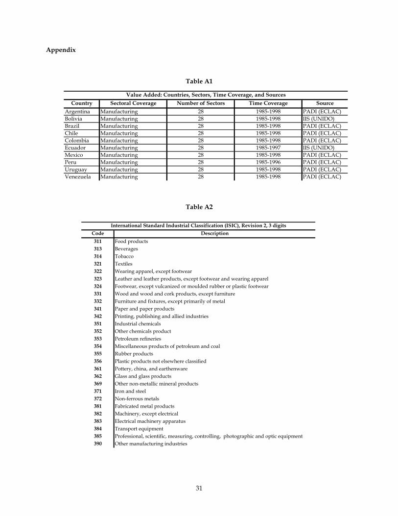
31

Appendix

Table A1

Table A2

Code Description311 Food products313 Beverages314 Tobacco321 Textiles322 Wearing apparel, except footwear323 Leather and leather products, except footwear and wearing apparel324 Footwear, except vulcanized or moulded rubber or plastic footwear331 Wood and wood and cork products, except furniture332 Furniture and fixtures, except primarily of metal341 Paper and paper products342 Printing, publishing and allied industries351 Industrial chemicals352 Other chemicals product353 Petroleum refineries354 Miscellaneous products of petroleum and coal355 Rubber products356 Plastic products not elsewhere classified361 Pottery, china, and earthenware362 Glass and glass products369 Other non-metallic mineral products371 Iron and steel372 Non-ferrous metals381 Fabricated metal products382 Machinery, except electrical383 Electrical machinery apparatus384 Transport equipment385 Professional, scientific, measuring, controlling, photographic and optic equipment390 Other manufacturing industries

International Standard Industrial Classification (ISIC), Revision 2, 3 digits

Country Sectoral Coverage Number of Sectors Time Coverage SourceArgentina Manufacturing 28 1985-1998 PADI (ECLAC)Bolivia Manufacturing 28 1985-1998 IIS (UNIDO)Brazil Manufacturing 28 1985-1998 PADI (ECLAC)Chile Manufacturing 28 1985-1998 PADI (ECLAC)Colombia Manufacturing 28 1985-1998 PADI (ECLAC)Ecuador Manufacturing 28 1985-1997 IIS (UNIDO)Mexico Manufacturing 28 1985-1998 PADI (ECLAC)Peru Manufacturing 28 1985-1996 PADI (ECLAC)Uruguay Manufacturing 28 1985-1998 PADI (ECLAC)Venezuela Manufacturing 28 1985-1998 PADI (ECLAC)

Value Added: Countries, Sectors, Time Coverage, and Sources

32

Table A3

Table A4

Country Variable Time Coverage SourceArgentina REERM 1987-1998 ECLAC

RERMIS 1985-1998 Terra and Valladares (2003)Bolivia REERM 1987-1998 ECLAC

RERMIS 1985-1998 Terra and Valladares (2003)Brazil REERM 1987-1998 ECLAC

RERMIS 1985-1998 Terra and Valladares (2003)Chile REERM 1987-1998 ECLAC

RERMIS 1985-1998 Terra and Valladares (2003)Colombia REERM 1987-1998 ECLAC

RERMIS 1985-1998 Terra and Valladares (2003)Ecuador REERM 1987-1998 ECLAC

RERMIS 1985-1994 Terra and Valladares (2003)Mexico REERM 1987-1998 ECLAC

RERMIS 1985-1998 Terra and Valladares (2003)Peru REERM 1987-1998 ECLAC

RERMIS 1985-1998 Terra and Valladares (2003)Uruguay REERM 1987-1998 ECLAC

RERMIS 1985-1998 Terra and Valladares (2003)Venezuela REERM 1987-1998 ECLAC

RERMIS 1985-1998 Terra and Valladares (2003)

Real Exchange Rate Measures: Countries, Time Coverage, and Sources

Country Variable Time Coverage SourceArgentina MFN 1985-1998 IDB/INT

PT 1985-1998 IDB/INTBolivia MFN 1985-1998 IDB/INT

PT 1985-1998 IDB/INTBrazil MFN 1985-1998 IDB/INT

PT 1985-1998 IDB/INTChile MFN 1985-1998 IDB/INT

PT 1985-1998 IDB/INTColombia MFN 1985-1998 IDB/INT

PT 1985-1998 IDB/INTEcuador MFN 1985-1998 IDB/INT

PT 1985-1998 IDB/INTMexico MFN 1985-1998 IDB/INT

PT 1985-1998 IDB/INTPeru MFN 1985-1998 IDB/INT

PT 1985-1998 IDB/INTUruguay MFN 1985-1998 IDB/INT

PT 1985-1998 IDB/INTVenezuela MFN 1985-1998 IDB/INT

PT 1985-1998 IDB/INT

MFN and Preferential Tariffs: Countries, Time Coverage, and Sources