Scale and ecological and historical determinants of a

species’ geographic range: The plant parasite

Phoradendron californicum Nutt. (Viscaceae)

By

Andrés Lira Noriega

Submitted to the graduate degree program in Ecology and Evolutionary Biology and the

Graduate Faculty of the University of Kansas in partial fulfillment of the requirements

for the degree of Doctor of Philosophy.

________________________________

Chairperson Jorge Soberón

________________________________

Chairperson A. Townsend Peterson

________________________________

Mark E. Mort

________________________________

Craig E. Martin

________________________________

Stephen L. Egbert

Date Defended: April 8, 2014

ii

The Dissertation Committee for Andrés Lira Noriega

certifies that this is the approved version of the following dissertation:

Scale and ecological and historical determinants of a

species’ geographic range: The plant parasite

Phoradendron californicum Nutt. (Viscaceae)

________________________________

Chairperson Jorge Soberón

________________________________

Chairperson A. Townsend Peterson

Date approved: April 8, 2014

iii

Abstract

Geographic ranges of species are fundamental units of study in ecology and

evolutionary biology, since they summarize views of how species’ populations and

individuals are organized in space and time. Here, I assess how abiotic and biotic factors

limit and constrain species’ geographic range, structure its distributions, and change in

importance at multiple spatial and temporal scales. I approach this challenge using

models and testable hypothesis frameworks in the context of ecological, geographic,

and historical conditions. Concentrating on a single species, the desert mistletoe,

Phoradendron californicum, I assess the relative importance of factors associated with

dispersal, host-parasite-vector niche overlap, and phylogeographic patterns for cpDNA

within a 6 mya timeframe and at local-to-regional geographic extents. Results from a

comparison of correlative and process-based modeling approaches at resolutions 1-50

km show that dispersal-related parameters are more relevant at finer resolutions (1–5

km), but that importance of extinction-related parameters did not change with scale.

Here, a clearer and more comprehensive mechanistic understanding was derived from

the process-based algorithm than can be obtained from correlative approaches. In a

range-wide analysis, niche comparisons among parasite, hosts, and dispersers

supported the parasite niche hypothesis, but not alternative hypotheses, suggesting

that mistletoe infections occur in non-random environmental subsets of host and

disperser ecological niches, but that different hosts get infected under similar climatic

conditions, basically where their distributions overlap that of the mistletoe. In a study of

iv

40 species, including insects, plants, birds, mammals, and worms distributed across the

globe, genetic diversity showed a negative relationship with distance to environmental

niche centroid, but no consistent relationship with distance to geographic range center.

Finally, P. californicum’s cpDNA phylogenetic/phylogeographic relationships were most

probable under a model of geologic events related to formation of the Baja California

Peninsula and seaways across it in the Pliocene and the Pleistocene; however, fossil

record, niche projections to the LGM, and haplotype distribution suggested shifting

distributions of host-mistletoe interactions and evidence of host races, which may

explain some of the genealogical history of the cpDNA. In sum, the chapters presented

here provide robust examples and methodologies applied to estimating the importance

and scale at which different sets of abiotic and biotic factors act to structure a species’

geographic range.

v

Acknowledgements

I wish to express my deepest gratitude to all of those who helped me throughout this

learning experience. I am indebted to my advisors Jorge Soberón and A. Townsend

Peterson for their unconditional support and friendship. From them I learned not only

how to think about science but about life.

I am grateful to my coauthors, committee members, and collaborators, and for

the scientific knowledge gained in working with them. Specifically, I wish to thank: Jorge

Soberón, Curtis P. Miller, A. Townsend Peterson, Joe Manthey, Oscar Toro, Jamie Oaks,

and Mark Mort. The support of my committee members throughout work on this

dissertation as well as other academic activities at KU was invaluable. This includes

guidance on remote sensing from Steve Egbert, on ecophysiology from Craig Martin, on

molecular work from Mark Mort. I feel privileged to count myself among the

collaborative team that developed from the Ecological Niche Modeling seminar. This

working group has been one of the most significant components of my academic

exercises at KU. From this group I thank Yoshinori Nakazawa, Alberto Jiménez-Valverde,

Sean Maher, Narayani Barve, Vijay Barve, Mona Papeş, Erin Saupe, Cori Myers, Hannah

Owens, and Peter Hosner. I also want to give special thanks to my friends and colleagues

Victor Baruch, Lindsay Campbell, Jesse Grismer, Carl Oliveros, Cam Siler, Charles Linkem,

and Fabricio Villalobos.

For their contributions to the fieldwork research presented in chapter 1, I am

grateful to Luis A. Sánchez-González, Gerardo Cendejas, Fran Recinas, and Rebecca

vi

Crosthwait. I wish to thank the personnel from several institutions and herbaria where

we stored specimens: Socorro González (Centro Interdisciplinario de Investigaciones

para el Desarrollo Integral Regional, Durango), Hilda Flores (Instituto de Biología,

UNAM), José Delgadillo (Universidad Autónoma de Baja California, Ensenada), and Jon

Rebman (San Diego Natural History Museum). I thank the curators and staff of the

following herbaria for providing access to their digital data: ARIZ, ASC, ASU, BCMEX,

BNHM, CANB, COCHISE, DES, GBIF, GCNP, IZTA, KANU, LL, MABA, MO, NMBCC, NY, RM,

SNM, TEX, UCR, UNM, USON, UTC, UVSC, XAL. I thank Luis Eguiarte and Mark Olson for

help with logistics, and the families of Gela and Alberto Búrquez, Sharon Herzka and

Juan Pablo Lazo, Socorro González, Gerardo Cendejas, and Rebecca Crosthwait for their

warm hospitality. Initial discussions about this work with Carlos Martínez del Río and

statistical guidance from Exequiel Ezcurra were crucial. I also thank A. Townsend

Peterson for insightful comments on this work and Narayani Barve for help with

weather values interpolation. Conversations with Richard Felger and Mark Robbins were

important to clarify points on climatic limiting factors and dispersal of the species.

For the work related to chapter 2 I thank Sean Maher for guidance on niche

overlap estimates, Mark Robbins for advice on potential mistletoe bird dispersers,

Richard Felger for help with species identifications and valuable comments on

background areas, and Ben Wilder for valuable comments on the manuscript.

For their comments on chapter 3, I thank John K. Kelly, Jorge Soberón, A.

Townsend Peterson, Lindsay P. Campbell, Jose Alexandre F. Diniz-Filho and three

anonymous reviewers who helped us to improve previous versions of this manuscript.

vii

For their contributions to chapter 4 I thank Ben Wilder for obtaining samples

from Isla del Tiburón and Isla Ángel de la Guarda; Richard Felger and Pedro Peña for

help with regionalization of the Sonoran Desert; and Jenny Archibald and Farzana

Ahmed for help with lab work and DNA extractions. Comments from A. Townsend

Peterson, Richard Glor, and Emily McTavish helped to improve previous version of the

manuscript. I thank curators from ASU for permission to sample loaned specimens as

well as Craig Freeman and Caleb Morse from KANU for supporting this project.

Scholarship support from Consejo Nacional de Ciencia y Tecnología, Mexico

(189216) enabled me to finance the first four years of studies at KU. Collecting trips

were possible thanks to financial support from a University of Kansas Biodiversity

Institute Panorama small grant award (Bunker Fund), a Tinker Award from the

University of Kansas Center of Latin American Studies, a Young Researchers Award from

the Global Biodiversity Information Facility (GBIF). Living expenses were also provided

by a scholarship from Secretaría de Educación Pública, Mexico, a Summer Research

grant in 2013 from the KU Department of Ecology & Evolutionary Biology, and grants

from JRS Biodiversity Foundation and the Instituto de Ecología, Xalapa, México

(SAGARPA-IICA-INECOL 2013). An Interdisciplinary Seed Grant from The Commons gave

me the opportunity to participate in one of the most enriching experiences—a

multidisciplinary research project with Ford Ballantyne IV, Donald Worster and Jorge

Soberón. Participation in conferences was possible thanks to financial support from the

KU Department of Ecology and Evolutionary Biology, the KU Office of Graduate Studies,

the KU Biodiversity Institute, the National Science Foundation’s IGERT Program at KU,

viii

and the Next Generation Sonoran Desert Researchers. A Marcia Brady Tucker Student

Travel Award funded travel to present research at the 127th AOU Meeting.

KU offered the best possible environment for this dissertation.

Special thanks to my friends Quica and Esteban Lerner, Monica Papeş and Arpi

Nyari, the Lira-Noriega foundation, the Campbell, Soberón and Peterson families, and

Emily Ryan for their support.

ix

Table of Contents

Abstract ............................................................................................................................... iii

Acknowledgements .............................................................................................................. v

Introduction ........................................................................................................................ 1

Process-based and correlative modeling of desert mistletoe distribution: A multiscalar approach ............................................................................................................................. 8

Abstract ....................................................................................................................................... 9

Introduction ............................................................................................................................... 10

Conceptual framework .......................................................................................................... 13

Methods .................................................................................................................................... 16

Distribution of species presences and landscape characteristics ......................................... 16

Host tree mapping ................................................................................................................. 18

Climate, host, and disperser summaries ............................................................................... 19

Process-based model ............................................................................................................. 21

Correlative models ................................................................................................................ 23

Model evaluations and comparisons .................................................................................... 24

Results ....................................................................................................................................... 26

Discussion .................................................................................................................................. 35

Acknowledgments ..................................................................................................................... 42

Range-wide ecological niche comparisons of parasite, hosts and dispersers in a vector-borne plant parasite system ............................................................................................. 44

Abstract ..................................................................................................................................... 45

Introduction ............................................................................................................................... 46

Materials and Methods ............................................................................................................. 50

Input data .............................................................................................................................. 50

Niche modelling ..................................................................................................................... 52

Niche similarity estimates ..................................................................................................... 54

Results ....................................................................................................................................... 56

Overall host and mistletoe-infected niche comparisons....................................................... 56

Disperser niche comparisons ................................................................................................ 59

Discussion .................................................................................................................................. 62

Acknowledgements ................................................................................................................... 67

Relationship of genetic diversity and niche centrality: A survey and analysis ................. 68

x

Abstract ..................................................................................................................................... 69

Introduction ............................................................................................................................... 69

Methods .................................................................................................................................... 74

Species’ occurrences and genetic diversity ........................................................................... 74

Niche characterization and distances to niche and geographic centroids ............................ 76

Results ....................................................................................................................................... 81

Discussion .................................................................................................................................. 89

Acknowledgements ................................................................................................................... 92

The roles of history and ecology in chloroplast phylogeographic patterns of the vector-borne plant parasite Phoradendron californicum Nutt. (Viscaceae) in the Sonoran Desert........................................................................................................................................... 93

Abstract ..................................................................................................................................... 94

Introduction ............................................................................................................................... 95

Materials and Methods ............................................................................................................. 97

Sampling ................................................................................................................................ 97

DNA extraction, amplification, and sequencing .................................................................... 99

Alignment and phylogenetic analyses ................................................................................. 100

Hypothesis testing in a phylogenetic context ..................................................................... 102

Ecological niche modeling ................................................................................................... 105

Host and mistletoe macrofossils ......................................................................................... 107

Results ..................................................................................................................................... 107

DNA sequences .................................................................................................................... 107

Gene tree reconstruction .................................................................................................... 108

Parsimony network ............................................................................................................. 109

Gene tree topology and ecological versus historical hypothesis testing ............................ 109

Present-Last Glacial Maximum suitability ........................................................................... 112

Host and mistletoe macrofossils ......................................................................................... 114

Discussion ................................................................................................................................ 116

Mistletoe phylogeny and phylogeographic patterns .......................................................... 116

Historical and ecological hypotheses .................................................................................. 118

Present and past distributions ............................................................................................ 121

Acknowledgments ................................................................................................................... 123

References ...................................................................................................................... 124

Appendices ...................................................................................................................... 143

Appendix 1.1 Derivation of the formulas for the process-based model. ................................ 143

xi

Table S1.1. Summary of model performance. ......................................................................... 146

Figure S1.1 Example binary maps for different models and sets of environmental. .............. 147

Figure S1.2 Example of map comparison with fuzzy Kappa statistic. ..................................... 148

Appendix 2.1 Model evaluation. ............................................................................................. 149

Appendix 3.1 Genetic diversity measures and estimates of distances to geographic range center and niche centroid. ...................................................................................................... 150

Appendix 4.1 Information on individuals and localities sampled in this study. Partitioning of individuals into populations according to each hypothesis (see Table 4.1) and DNA sequences GenBank accession numbers. .................................................................................................. 151

Appendix 4.2. Methods to obtain the layers on the historical, ecological, and geographic conditions used for population partitioning in the Bayesian coalescent analysis. ................. 161

Appendix 4.3 Packrat midden localities from western North America with hosts and mistletoe macrofossil information. ......................................................................................................... 164

Appendix 4.4 Model evaluation. ............................................................................................. 165

Table S4.1 Results from delimitation of lineages using the ML GMYC method. ..................... 166

Table S4.2 Marginal likelihood and Bayes factor of the hypotheses used to test the phylogenetic relationships of the gene tree without population 225 (see Table 4.1). ........... 167

Table S4.3 Levels of nucleotide variability per sequenced chloroplast region. ...................... 168

Figure S4.1 Phoradendron californicum haplotype network and potential distribution for mistletoe (inset) and hosts distributions during the LGM (21 kya) according to the CCSM climate scenario. ..................................................................................................................... 169

Figure S4.2 Haplotype network configuration on concatenated data sets including two cpDNA regions. .................................................................................................................................... 170

1

Introduction

The ways in which species are formed, the changes of their geographic ranges through

time and the role of environmental conditions on those ranges are issues that have

always been central to the study of biodiversity. Since the publication of the works by

Darwin (1857) and Wallace (1858), and later with studies on species ecological niches,

evolution and interactions (Elton 1927, Grinnell 1917, Hutchinson 1957), it has become

clear that species distributions are affected by a variety of physical and biological factors,

and that this mosaic of conditions is constantly changing and influencing species

behavior, abundance and evolution (Darwin 1859, Andrewartha and Birch 1954, Udvardy

1969, Darlington 1957, MacArthur 1972, Mayr 1963). These factors include the

geographic configuration and change of continents, islands and oceans, since they may

act as barriers or conduits for dispersal; their climates, soils, and habitats; and the

fluctuations in the abundance of those species that interact in a positive or negative way

with a given species.

Geographic ranges of species are fundamental units of study in ecology and

evolutionary biology since they summarize how species’ populations and individuals are

organized in space and time (Gaston 2003). Historically, this led scientists to ask questions

about: (1) the conditions that allow populations to maintain a positive growth rate, and

(2) the impacts that individuals from such populations have on their environment

(Hutchinson 1957, 1978, Chase and Leibold 2000). The study of geographic ranges is

formed by multiple research programs. Many of these are characterized by the search for

2

general patterns of species distributions and associations looking at statistical

relationships to explain the distribution of biodiversity at large scales, based on the idea

that small-scale local processes alone were not able to fully explain the abundance and

distribution of species. Examples of such approaches include the field of ‘areography,’

interested in the description of the structure and position of the ranges (Rapoport 1982),

and that of ‘macroecology,’ which focuses on large-scale description of patterns of

abundances across and on the associations of species incorporating their physiological

requirements in relation to body size (Brown and Maurer 1989). These approaches,

however, usually lack a mechanistic explanation for the patterns and can only generalize

on the distributional patterns based on correlative approaches, although this situation is

currently changing (Keith et al. 2012).

These ‘non-experimental’ approaches are informed by a plethora of observations

and field experiments, in many ways similar to the keen observations of distributional

patterns and of the effect of changes in scale we find in Darwin’s work. Despite so much

accumulated research, estimating a species’ geographic distribution and its limiting

factors in space and time is still a challenge, and a priority, given the need to estimate

biodiversity under current and future conditions and understanding the processes that

generate it.

The estimation of the distribution of species from the perspective of which

environmental conditions permit their existence (niches, or Grinnellian niches, when

conditions are restricted to certain classes of variables) has been extremely fruitful. When

studying species’ distributions and niches, it is useful to distinguish interacting variables

3

(bionomic variables) from those that are dynamically uncoupled from the presence or

abundance of the species in question (scenopoetic variables; Hutchinson 1989, Soberón

2007). These variables may have contrasting effects at fine versus coarse spatial

resolutions (Wiens 1989, Levin 1992). The many ways in which scenopoetic variables

operate at different extents and resolutions can be used to explain distributions of the

species and propose scale-dependent hypotheses regarding factors most relevant at

different scales (Pulliam 2000, Gaston 2003, Soberón and Peterson 2005, Soberón 2007,

2010, Peterson et al. 2011).

In the chapters presented here, I use information on the natural history of a small

set of interacting species to hypothesize how different configurations among the causal

factors underlying geographic distributions of species, in the heuristic device called BAM

diagram (Soberón and Peterson 2005, Peterson et al. 2011), act at different spatial scales.

The BAM diagram displays relationships between abiotic or uncoupled (A) and coupled

biotic factors (B), and the movement or dispersal capacities of the species (M). This

framework can be used to make explicit the possible arrangements of factors that

determine distributions of species, and gives the opportunity to generate hypothetical

scenarios, depending on the degree and geometry of their overlap (see Fig. 1.2).

Specifically, with this framework, we can analyze interactions of factors at fine and coarse

spatial resolutions (Peterson et al. 2011). As a complement to this framework, I conduct

analysis and comparisons with methods used in ecology and systematics. Such a

multidisciplinary approach allowed me to understand the patterns and processes

underlying the distribution and maintenance of species populations at multiple scales.

4

Here I explore how factors that limit a species’ range are structured at multiple

spatial and temporal scales. In particular, I ask how biotic and abiotic factors change in

importance depending on the spatial and temporal scale at which they are measured. To

do this, I build models and testable frameworks for hypotheses in the context of

ecological, geographic, and historical conditions limiting and structuring a species range

and its genetic diversity and relationships.

For most of the dissertation (chapters 1, 2, and 4), I concentrate primarily on a

single species, the desert mistletoe, Phoradendron californicum Nutt. (Viscaceae). This

allowed me to optimize data acquisition and modelling across a species’ geographic

range. In particular, I take advantage of the vector-borne parasitic nature of the species

to understand the relative importance of scenopoetic variables and dispersal, and the

overall role of hosts and dispersers in limiting the species geographic range. This research

builds upon previously published work, most of it collected at local scales (a few hectares;

e.g., Overton 1997, Aukema 2001), and generalizes the influence of scenopoetic variables,

interaction with hosts and dispersal on the expansion and contraction of the species

range since 6 mya. A fourth chapter (chapter 3) uses published information on genetic

diversity for 40 species which include plants, insects, birds, mammals, and worms, to test

the relationship of the abundant-center hypothesis in terms of niche centrality and

geographic centrality.

In chapter 1 I explore how dispersal and scenopoetic factors act synergistically to

explain the distribution of P. californicum, at five spatial resolutions (1, 5, 10, 20, 50 km). I

compare correlative niche modeling methods (GARP, Maxent, GAM) with a process-based

5

model derived from a metapopulation-dynamic framework coupling rates of colonization

and extinction. I hypothesize that, as resolution coarsens, variables associated with

abiotic factors (climate) will become more important, but that the opposite will apply for

biotic variables (dispersal). I developed analyses within the distributional area of the

disperser species. Results show that correlative models improved when layers associated

with hosts and disperser were used as predictors, in comparison with models based on

climate only; however, they tended to overfit to data as more layers were added.

Dispersal-related parameters were more relevant at finer resolutions (1–5 km), but the

importance of extinction-related parameters did not change with scale. I observed

greater coincidence between correlative and process-based models when based only on

dimensions of the abiotic niche (climate), but a clearer and more comprehensive

mechanistic understanding was derived from the process-based algorithm.

In chapter 2 I test whether the distribution of the mistletoe P. californicum is

mediated by host distributions (host niche hypothesis, HNH), or by factors such as the

mistletoe’s autecology (parasite niche hypothesis, PNH) or that of its vectors (vector niche

hypothesis, VNH). The null hypothesis is that the ecological niche of the mistletoe will not

be distinct from that of its hosts or vectors; alternatively, mistletoe infections might

appear in hosts only in regions where host distributions overlap suitable conditions for

the parasite. To do this I used ecological niche modelling approaches to summarize

suitable environmental conditions for hosts infected and uninfected with mistletoes, as

well as for avian dispersers during winter and throughout the year. I compared ecological

niches among pairs of species using background similarity tests in relation to the climatic

6

conditions available and accessible to each species. Niche comparisons supported all PNH

expectations but none of the predictions of HNH or VNH. This suggests that hosts and

dispersers of mistletoes generally have distinct ecological niches, that mistletoe infections

occur in non-random environmental subsets of host and disperser ecological niches, but

that mistletoe infections in different hosts, occur under similar climatic conditions. Thus,

in this system, the parasite has a rather strictly circumscribed ecological niche, and host

species become infected with mistletoe only where they overlap its suitable areas.

In chapter 3 I tested whether the abundant-center hypothesis for ecological

niches (Martinez-Meyer et al. 2013) would hold for genetic diversity. One hypothesis

predicts that natural populations at geographic range margins will have lower genetic

diversity relative to those located centrally in species’ distributions due to a link between

geographic and environmental marginality; alternatively, genetic variation may be

unrelated with geographic marginality via decoupling of geographic and environmental

marginality. I investigate the predictivity of geographic patterns of genetic variation based

on geographic and environmental marginality using published genetic diversity data for

40 species (insects, plants, birds, mammals, worms). Results showed that only about half

of species showed positive relationships between geographic and environmental

marginality. Three analyses (sign test, multiple linear regression, and meta-analysis of

correlation effect sizes) showed a negative relationship between genetic diversity and

distance to environmental niche centroid but no consistent relationship of genetic

diversity with distance to geographic range center.

7

In chapter 4 I tested how different ecological and historical (vicariant) factors

shape distributions of individuals and genes in P. californicum. I first describe the

phylogeographic patterns based on three non-coding chloroplast DNA regions and assess

the marginal probability of 16 a priori hypotheses related to geologic events and

ecological factors in order to predict the cpDNA variation across the geographic range of

the species within a Bayesian phylogenetic framework. Complementarily, I use

macrofossil record from packrat middens and niche model projections on Last Glacial

Maximum climatic conditions for hosts, mistletoe, and a bird specialist to interpret

phylogeographic patterns. Results show that patterns of variation in cpDNA haplotypes

are most probable under a model reflecting a series of geologic events related to

formation of the Baja California Peninsula and seaways across it in the Pliocene and the

Pleistocene. Alternatively, fossil record, niche projections, and haplotype distribution

suggested shifting distributions of host-mistletoe interactions and evidence of host races,

which might explain some of the genealogical history of the cpDNA; however, these

hypotheses were not favored by the Bayesian statistical tests. Depending on molecular

rate, age estimates for well-supported nodes were compatible with geologic events or

climatic oscillations. Our findings suggest that variation of cpDNA across the species range

results from the interplay of vicariant events, past climatic oscillations, and more dynamic

factors related to ecological processes at finer scales.

8

Chapter 1

Process-based and correlative modeling of desert

mistletoe distribution: A multiscalar approach1

1 Lira-Noriega A, Soberón J, Miller CP (2013) Process-based and correlative modeling of desert mistletoe distribution: A multiscalar approach. Ecosphere 4, art99.

9

Abstract

Because factors affecting distributional areas of species change as scale (extent and grain)

changes, different environmental and biological factors must be integrated across

geographic ranges at different resolutions, to understand fully the patterns and processes

underlying species’ ranges. We expected climate factors to be more important at coarse

resolutions and biotic factors at finer resolutions. We used data on occurrence of a

parasitic plant (Phoradendron californicum), restricted to parts of the Sonoran and

Mojave deserts, to analyze how climate and mobility factors explain its distributional

area. We developed analyses at five spatial resolutions (1, 5, 10, 20, 50 km) within the

distributional area of the disperser species, and compared ecological niche models from

three commonly used correlative methods with a process-based model that estimates

colonization and extinction rates in a metapopulation framework. Correlative models

improved when layers associated with hosts and disperser were used as predictors, in

comparison with models based on climate only; however, they tended to overfit to data

as more layers were added. Dispersal-related parameters were more relevant at finer

resolutions (1-5 km), but importance of extinction-related parameters did not change

with scale. We observed greater coincidence between correlative and process-based

models when based only on dimensions of the abiotic niche (i.e., climate), but a clearer

and more comprehensive mechanistic understanding was derived from the process-based

algorithm.

10

Introduction

The relative roles of biotic and abiotic factors in determining distributions of species at

specific spatial scales are a central organizing theme in ecology (Levin 1992).

Understanding how patterns at one scale are manifestations of or influence processes

operating at other scales is a particular challenge (Levin and Pacala 1997, Pearson and

Dawson 2003, Hastings et al. 2010). The core of this challenge lies in disentangling how

changes in scale affect the importance of different factors in shaping species’

distributional patterns and processes.

When studying species’ distributions, it is useful to distinguish interacting

variables from those that are dynamically uncoupled from the presence or abundance of

the species in question (scenopoetic variables; Hutchinson 1978). These variables may

have contrasting effects at fine versus coarse spatial resolutions (Wiens 1989). The many

ways in which scenopoetic variables operate at different extents and resolutions can be

used to explain distributions of the species and propose scale-dependent hypotheses

regarding factors most relevant at different scales (Pulliam 2000, Gaston 2003, Soberón

and Peterson 2005, Soberón 2007, 2010, Peterson et al. 2011).

Using data available documenting species’ occurrence and climatic variation,

researchers have been able to estimate environmental requirements of many species

across broad regions (Guisan and Zimmermann 2000, Elith et al. 2006). Factors

manifested at finer resolutions are less well studied at the scope of broad geographic

ranges, leaving a gap in understanding as to how effects of these factors vary spatially

and temporally. Also, knowledge of species’ distributions at local scales may be sparse or

11

biased spatially across geographic ranges, which makes analyzing the relative importance

of variables even more difficult (MacArthur 1972, Levin 1992). These considerations

explain why studies of spatial distributions of species that combine broad-scale and fine-

scale views remain uncommon (e.g., Mackey and Lindenmayer 2001, Gaston et al. 2004,

Heikkinen et al. 2007, Cunningham et al. 2009).

Correlative and process-based modeling are two approaches for exploring factors

important in determining distributions of species at different spatial scales (Robertson et

al. 2003, Kearney et al. 2010). The main difference between these approaches is that

correlative methods simply seek associations between environments and occurrences

from across broad geographic ranges, whereas process-based methods incorporate

explicit hypotheses about biological processes (Robertson et al. 2003, Kearney and Porter

2009, Monahan 2009, Morin and Thuiller 2009, Cabral and Schurr 2010, Kearney et al.

2010). In particular, a set of factors that is emerging as crucial in process-based modeling

studies is dispersal: incorporating dispersal factors improves model performance

markedly (Allouche et al. 2008, Cabral and Schur 2011, Brotons et al. 2012).

In this paper, we explore how dispersal and scenopoetic factors act synergistically

to explain the distribution of the Desert Mistletoe, Phoradendron californicum, at varying

spatial resolutions. P. californicum is a hemi-parasitic plant associated with legume hosts

in the Sonoran and Mojave deserts, and it is dispersed in largest part by the bird species

Phainopepla nitens (Walsberg 1975, Kuijt 2003). This parasite-host-disperser system

offers two advantages for understanding how scaling of biological processes govern

distributions (Overton 1996, Aukema and Martínez del Rio 2002, Aukema 2003, 2004): (1)

12

hosts are known, and their distributions can be studied at high spatial resolution using

aerial photographs; and (2) dispersal is determined chiefly by a single disperser. We

modeled the portion of the distribution of P. californicum in the U.S., where detailed data

on Phainopepla nitens are available (almost 900,000 km2; Fig. 1.1), encompassing

approximately half of the parasite species’ range. We compare commonly-used

correlative niche modeling methods (GARP, Maxent, GAM) with a process-based model

derived from a metapopulation-dynamic framework coupling rates of colonization and

extinction. Following Pearson and Dawson (2003) and others, we hypothesize that, as

resolution coarsens, variables associated with abiotic factors (e.g., climate) will become

more important, but that the opposite will apply for biotic variables (e.g., dispersal).

13

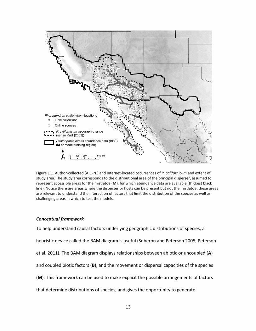
Figure 1.1. Author-collected (A.L.-N.) and Internet-located occurrences of P. californicum and extent of study area. The study area corresponds to the distributional area of the principal disperser, assumed to represent accessible areas for the mistletoe (M), for which abundance data are available (thickest black line). Notice there are areas where the disperser or hosts can be present but not the mistletoe; these areas are relevant to understand the interaction of factors that limit the distribution of the species as well as challenging areas in which to test the models.

Conceptual framework

To help understand causal factors underlying geographic distributions of species, a

heuristic device called the BAM diagram is useful (Soberón and Peterson 2005, Peterson

et al. 2011). The BAM diagram displays relationships between abiotic or uncoupled (A)

and coupled biotic factors (B), and the movement or dispersal capacities of the species

(M). This framework can be used to make explicit the possible arrangements of factors

that determine distributions of species, and gives the opportunity to generate

14

hypothetical scenarios, depending on the degree and geometry of their overlap (Fig. 1.2).

Specifically, with this framework, we can analyze interactions of factors at fine and coarse

spatial resolutions.

Figure 1.2. Conceptual framework showing (a) the relationship between biotic-abiotic-mobility (BAM) conditions for a species to be present. (b) Interpretation of the BAM diagram in this modeling exercise restricts to the use of abiotic conditions (A) and accessible areas (M), assuming that the interaction between host and parasite is uncoupled, and that the positive interaction between disperser and parasite makes biotic conditions (B) and accessible area (M) coincident. As scale changes, limiting factors in A and M will also change. At higher resolutions, almost the entire area is accessible, and climate is not so limiting, whereas at coarser resolutions dispersal becomes more difficult and climate is more constant.

In the mistletoe-host-disperser system, the BAM diagram can be simplified

significantly by making some reasonable assumptions. The conditions manifested across

A (Soberón and Peterson 2005, Soberón 2007) represent those under which the species

can have a positive growth rate (Hutchinson 1978); therefore, conditions in A are linked

intimately to the environmental dimensions on which mechanisms of establishment and

survivorship depend (Wiens 2000). Factors in M are related to movement: what happens

across M determines how populations will be structured, demographically and

15

genetically, although testing this particular idea will be accomplished in a later phase of

this project (Lira-Noriega et al. in prep).

We hypothesize that, to a first degree of approximation, the interaction with the

host can be regarded as uncoupled, since hosts have expected lifetimes at least 10-fold

longer than those of parasites (Overton 1996, 1997) and therefore their population

dynamics can be regarded as approximately static relative to the faster demography of

the parasites. The simplifying assumption of uncoupled dynamics of the total host

population is often made in epidemiological studies (Anderson, 1981). This means that we

regard climate and presence of hosts as part of the A circle. Second, we did not include

the effect of competitors, which are not known to be present, nor of herbivores or

pollinators, because information about them at the spatial extent of our study is simply

unavailable.

Finally, in the mistletoe system, one major biotic factor, birds, act directly as

dispersers. From a certain point of view the dispersers may be considered as part of B,

but their effect is clearly felt in the dispersal circle, making B and M coincident. In

consequence, we can simplify our system to a two-factor diagram: the abiotic climatic

factors (A) and the hosts substrate, that determine overall potential distributions, and the

movement or dispersal capacity of the species (M), driven mainly by the bird that

disperses seeds among trees. M represents a hypothesis of the regions that have been

accessible for the species over relevant time periods; as such, M is the area across which

models should be calibrated (Barve et al. 2011; see also Acevedo et al. 2012). Following

this reasoning, we designated an M as the area of distribution of the mistletoe’s main

16

disperser, P. nitens, for which we have detailed abundance information (Fig. 1.1).

Although other potential dispersers of the mistletoe species in question are known, none

is as closely associated as this species (Walsberg 1975); adding the densities of other bird

species to the model would not have changed our results, given that they overlap broadly

in their distribution and behavior with that of P. nitens. This assumption can be relaxed in

future studies, but for the present simplifies the process-based modeling exercise

considerably.

Methods

We designed a comparison of a process-based model with correlative models from three

algorithms to understand the distribution of P. californicum at five spatial resolutions (1,

5, 10, 20, 50 km). We first describe the series of steps we followed in order to obtain data

on the distribution of the parasite followed by the assemblage of three sets of

environmental variables: spatial variation in disperser density, spatial variation in

numbers of hosts, and climatic factors across the study area. We then describe the design

and implementation of each model type and finally the comparisons among them.

Distribution of species presences and landscape characteristics

To estimate proportions of mistletoe-infected trees, we recorded geographic locations of

infected host trees along roads. One of us (A.L.-N.) sampled occurrences of host trees

infected by P. californicum across the southwestern United States and northwestern

Mexico (Fig. 1.1). We used roads as sampling transects as an efficient means of surveying

the species’ range limits, allowing us to gather information regarding the broader set of

17

climatic situations where the species occurs. We used a GPS unit to record geographic

coordinates for each infected host tree located within 100 m of the road. In total, we

sampled 16,000 km (4153 km within the modeling extent) of roads, and collected 17,371

unique geographic coordinates of infected trees (Fig. 1.1), 12,578 of which fell within the

modeling extent (see below).

Sampling along roads may potentially bias the data, since roads are usually areas

of higher water accumulation, thus impacting quality of the hosts (Norton and Smith

1999). However, given that we are generalizing prevalence of the species from host trees

at several spatial resolutions (cells of 1, 5, 10, 20 and 50 km by side), we assume that the

effect of roads is constant and will not influence our general understanding of mistletoe

distributions. Identification of host and mistletoe species was achieved via collection of

herbarium specimens at sites every ~50 km across the study area or every time changes

in host species composition were suspected. We used a second GPS unit to record

landmarks by which to annotate general descriptions of species composition and

vegetation physiognomy and landscape characteristics along the road; this information

was used in processing aerial photographs (see below). All voucher specimens are

deposited at the Ronald L. McGregor Herbarium, University of Kansas; copies of the

collection were deposited at different herbaria in Mexico and the United States (see

Acknowledgements). The two GPS units were Garmin 60CSx, with antennas to improve

precision of coordinate estimates.

18

Host tree mapping

To derive proportions of infected trees for the process-based model, we extracted

geographic coordinates of tree canopies along roads sampled. This step was achieved

using National Agriculture Imagery Program (NAIP) aerial photographs, ideal for tree

mapping because of their high spatial and spectral resolution (1 m and four bands—red,

green, blue, and near infrared). We carried out object-oriented classification of these

photographs with the software eCognition 3.0 (Baatz et al. 2003). We first identified all

3.75’ x 3.75’ aerial photographs that intersected the roads sampled. We further reduced

the set of aerial photographs to those including the land use cover types in which

mistletoe infections were found via comparisons with the 2001 National Land Cover

Database (30 m resolution; Homer et al. 2004); land cover types considered were barren

land, cultivated land, deciduous forest, development low density, development medium

intensity, development open space, emergent herbaceous wetlands, hay/pasture,

herbaceous, open water, shrub/scrub, and woody wetlands. We selected at random 10%

(67) of the aerial photographs for the states of Arizona (25; from 2007), New Mexico (6;

2009), California (13; 2009), and Nevada (23; 2006). Because of significant computational

demands in the classification process, each 3.75’ x 3.75’ image was split into four equal

portions for processing, generating a total of 268 images to classify.

In eCognition, we first segmented each image into two levels, with the following

parameters: level 1 (scale = 10, color = 0.8, shape = 0.2, smoothness and compactness =

0.5) and level 2 (scale = 3, color = 0.8, shape = 0.2, smoothness and compactness = 0.5).

Then, to classify trees, we selected polygons manually from the level 2 objects to be used

19

as canopy samples, and classified each image using the standard nearest neighbor with

the mean of each of the four bands (R, G, B, and NIR), the mean difference from

neighbors, and the mean difference between the level 2 objects nested within the level 1

super-object. These procedures have been used in previous studies that have analyzed

mesquite distributions in similar landscapes and regions (e.g., Laliberte et al. 2004). Using

ArcGIS 9.3, we dissolved the raw polygon output from eCognition to obtain single-tree

polygons. This step was necessary because the output sometimes contained multiple

polygons subdividing single tree crowns. Although this procedure sometimes reduced

numbers of trees estimated, it was not a common problem overall, and estimates of trees

were close to true numbers of trees in each image (R2 = 0.617, P < 0.001). This step

allowed us to extract 5,786,586 polygons corresponding to tree crowns, and count actual

numbers of trees within the 200 m strip along roads, to estimate proportions of trees

infected (via the GPS coordinates of mistletoes described above).

Climate, host, and disperser summaries

These datasets were each derived at five spatial resolutions, as follows. Climatic layers

used were annual mean temperature and annual precipitation, obtained from the

WorldClim database (Hijmans et al. 2005), using the 30”, 2.5’, 5’, and 10’ resolution

products to match 1 km, 5 km, 10 km, and 20 km resolutions, respectively; for the 50 km

resolution, we scaled the values up with the mean of the 10’ raster layers using a bilinear

interpolation from nearest neighbor cells. Because other climatic factors, particularly

freezing temperatures and sunny days, can be important limiting factors for the

mistletoe, we tested models with two other variables estimated directly from weather-

20

station data (Easterling et al. 1999) for a 20-yr period (number of continuous days of

freezing temperatures and number of continuous rainless days). Because models

resulting showed similar or lower performance scores, these variables were not included

in our final analyses.

The raster data layer summarizing abundances of Phainopepla nitens was

obtained from the Breeding Bird Survey database (v.12.07.2011 [Sauer et al. 2011]),

which comes as a vector-format data layer with cells at a resolution of 25 km, the product

of interpolating point abundance information across the bird species’ distribution in the

United States. In contrast to the rest of the layers used for modeling, this data layer was

used statically at its native resolution (i.e., not scale-dependent) for the first four

resolutions of our analyses.

To estimate numbers of host trees across the region, we developed models to

predict numbers of trees per cell at 1 km resolution using random forests (randomForest

in R; Liaw and Wiener 2002). This estimate was based on 580 1-km cells sampled across

the region from 85 images from the NAIP (55 images from Arizona, 7 from New Mexico, 7

from California, and 16 from Nevada) that were classified following the protocol

described above. Specifically, we asked for a total of 10,000 trees developed under the

random forest protocol, from which we estimated the logarithm of the number of host

trees with the following statistical model: log 10 of host trees ~ GRS 2000 + NVG 2000 +

annual mean temperature + annual precipitation + maximum temperature of the

warmest month + precipitation of the wettest month + slope + elevation + aspect +

latitude + longitude. The grass/scrub/woodland (GRS 2000) and barren/very sparsely

21

vegetated land (NVG 2000) are raster data layers obtained from the Harmonized World

Soil Database v 1.1 (Fischer et al. 2008). The final estimate of the number of host trees

was more explanatory (67.0% of total variation) and showed better fit between observed

and predicted numbers of trees (r = 0.91, P < 0.01) and between observed and

independent external data set aside from the classified images (r = 0.60, P < 0.01) than

other random forests based on different combinations of variables, numbers of

observations, and numbers of trees within the process. This procedure also gave better

results than the two most explanatory (67.7−68.1% of total variation) generalized additive

models (GAMs) of different combinations of same predictors as used in the random forest

(r = -0.22, P > 0.01; r = -0.16, P > 0.01). Although the explained variances are similar, the

shape of the relationship in the random forests is more regular and linear than with the

GAMs.

Process-based model

To estimate probability of occurrence of P. californicum in grid cells via a process-based

modeling approach, we developed a spatially explicit model incorporating the balancing

rates of colonization and local extinction, as proposed in the theory of metapopulations

(Hanski 1999, Vandermeer and Goldberg 2003, Roberts and Hamann 2012). The model

was developed as follows.

After some assumptions related to using a mean-field approximation, we fit the

following equation following Hanski’s (1999) incidence function model:

22

JJ

J J

cp

c e

,

where Jp represents the proportion of hosts in a composite cell J occupied by mistletoes.

The parameter Jc is the mean colonization rate, assumed to be a function of the density

of birds and host trees in the focal cell J and neighboring cells. The parameter Je is the

mean death rate of mistletoes, assumed to be a function of the distance between optimal

climate, as estimated as the difference of average climatic conditions across known

occurrence points (for each resolution) and the climate in the cell J. This model was fit for

each of the five spatial resolutions using a maximum likelihood routine implemented in R.

Derivations of formulas for this model are provided in Appendix 1.1.

To estimate variability in parameters, we resampled the data with replacement

115 times to obtain a distribution of colonization and extinction-related parameter values

with the following number of observations in each iteration: 200 (56% of the original data

matrix) at 1 km resolution, 70 (63%) at 5 km, 50 (68%) at 10 km, 30 (54%) at 20 km, and

20 (64%) at 50 km. The distributions obtained were used to assess whether parameters

differed from zero, and how different they were among scales, using t-tests. Specifically,

we evaluated two colonization parameters, disperser abundance and disperser cost of

movement across neighboring cells; in the extinction formula, we tested the deviation

from a climate optimum as defined by Mahalanobis distance to the environments in the

occurrence points for each resolution (see Appendix 1.1).

23

Correlative models

We ran a total of 45 correlative models: three algorithms, three sets of environmental

predictors, and five spatial resolutions. We used two presence-background correlative

niche-modeling algorithms: DesktopGARP (best subsets version in OpenModeller v.1.1.0;

de Souza Muñoz et al. 2011) and Maxent v.3.3.3 (Phillips et al. 2006), as well as the

presence-absence algorithm generalized additive models (GAM; mgcv [Wood 2011]). We

set parameters in GARP as follows: occurrence data for training 50%, soft omission

threshold, 100 replicate runs, and best subsets option; the rest of the settings were as

default. In Maxent, we set 50% of occurrence points for model calibration, and chose

logistic output; the rest of settings were as default. To run models, we selected 5% (N =

629) of the total number of infected trees, after considering the spatial lag of spatial

autocorrelations in environmental characteristics as follows. The spatial lag was

estimated on the first principal component of the 19 bioclimatic variables as a surrogate

for the environmental space in the study region. Principal components were calculated

using a correlation matrix in R (stats; R Development Core Team 2011) and the spatial lag

was estimated as the distance associated with the sill of a semivariogram in the package

Spatial Analysis in Macroecology (SAM 4.0; Rangel et al. 2010). We then sampled the 5%

of the occurrence points subject to the constraint that they be separated by at least that

distance in space.

We explored influences of different environmental factors on the distribution of P.

californicum in correlative models using three sets of variables: (1) annual mean

temperature and annual precipitation (“climate”); (2) abundance of Phainopepla nitens

24

and numbers of host trees (“disperser + host”); and (3) a combination of all three

(“climate + disperser + host”). All models were trained and projected within the extent

that corresponds to the distribution of the disperser (M) at each spatial resolution. The

importance of environmental predictors at each scale was estimated using the jackknife

of regularized training gain in Maxent, recalculation of GARP accuracy using jacknife in

openModeller, and the P-value for significance of each variable in GAMs. These

procedures form part of the output of each algorithm.

Model evaluations and comparisons

All 50 models (45 correlative and 5 process-based) were evaluated using the partial AUC

approaches implemented by Peterson et al. (2008), using 262 independent unique

occurrence points for P. californicum from the Global Biodiversity Information Facility

(www.gbif.org; search in September 2010). This procedure allowed us to evaluate

performance of each model as compared to random expectations, as well as to compare

performance across scales and modeling methods. Partial AUC approaches limit analysis

to portions of the ROC curve that are relevant to the question at hand (i.e., within

omission error tolerances); so one calculates the ratio between the area under the curve

for observed values against the area under the line of random discrimination, AUC ratios

are expected to depart upwards from one as model performance is better than random.

The main advantage of this procedure is that the comparison covers only the range of

values over which each algorithm predicts, thus avoiding problem caused by using equal

scales of values when such is not the case in all comparisons (e.g., Maxent and GARP;

Peterson et al. 2008).

25

To do this testing, we first multiplied grids by 1000, and converted each floating-

point grid to an integer grid in ArcGIS 10. Using the modeled suitability values associated

with each independent testing point, we implemented partial AUCs by running 1000

bootstrap simulations in a Visual Basic program (Barve, www.biodiversity-informatics-

training.org), with 50% of points resampled with replacement in each iteration of the

bootstrap, and E = 0.05, given that these testing occurrences were obtained from GBIF

and may be subject to some georeferencing or identification error. Distributions of the

randomized ratios were compared with z-tests to see if ratios were consistently larger

than 1 (1 corresponds to random discrimination). The ratios that resulted from this

procedure were also used to compare models in a three-way ANOVA for type of

algorithm, environmental predictors, resolution, and interactions of these three factors

using R (stats; R Development Core Team 2008).

The degree of spatial agreement between model predictions was calculated using

a fuzzy Kappa statistic in the software Map Comparison Kit (Visser and de Nijs 2006), and

Pearson and Spearman correlations were estimated between 3000 random points for

resolutions 1-20 km and between the 527 pixels at the 50 km resolution following the

Dutilleul method to correct for spatial autocorrelation in SAM 4.0 (Rangel et al. 2010),

which corrects the number of degrees of freedom of estimated variances. Kappa statistics

were calculated for models thresholded using the minimum training presence value (Liu

et al. 2005, Wilson et al. 2005), given that we are confident that occurrence points used

for model calibration correspond to a P. californicum with no error (E = 0). Finally, we

26

compared the area predicted as suitable for each model using boxplots to examine

effects of model type, environmental predictors, and spatial resolution visually.

Results

All models, except for a marginally lower result in the 1 km process-based model,

performed better than random expectations when tested against independent

occurrence points (all P < 0.05; Table S1.1). Comparisons of model performance using

AUC ratios indicated differences in performance of models depending on the algorithm,

environmental predictors, and resolution, as well as interactions among these factors

(Table 1.1). At all resolutions, the lowest AUC ratios were for models using climate only as

environmental predictors; AUC ratios were in general higher for models with disperser +

host and climate + disperser + host environmental predictors alone (Fig. 1.3). AUC ratios

at resolutions of 1 and 5 km were highest when the environmental predictors were

climate + disperser + host, followed by the AUC ratios when the environmental predictors

were disperser + host, and comparatively lower AUC ratios when the environmental

predictor was climate (Fig. 1.3). AUC ratios at resolutions of 10 and 20 km had lower

mean ratios when the whole set of predictors were used. At the coarsest resolution (50

km), AUC ratios remained low for climate and disperser + host, but were considerably

higher for climate + disperser + host (Fig. 1.3).

27

Table 1.1. Three-way ANOVA on partial AUC ratios using as factors the different sets of variables (“climate”, “disperser + host”, “climate + disperser + host”), algorithms (process-based, GARP, Maxent, GAM), and resolutions (1, 5, 10, 20, 50 km), including interactions among factors. All comparisons were significantly different at P < 10-15.

Sum of squares d.f. F

Algorithm 184.031 3 16981.19 Resolution 11.253 4 778.75 Variables 110.021 2 15228.07 Algorithm : Resolution 55.616 11 1399.61 Algorithm : Variables 32.411 4 2243.01 Resolution : Variables 39.347 8 1361.5 Algorithm : Resolution : Variables 49.288 16 852.74 Residuals 177.01 49,000

Figure 1.3. Interaction plot of AUC ratios after 1000 iterations in the partial ROC based on independent occurrences of Phoradendron californicum. Differences in model performances are statistically significant (P < 0.001). Process-based model results were included in the set of variables “climate + disperser + host.”

Coincidence among models, after converting them to binary maps, was highly

variable in terms of both amount of area predicted as suitable and amount of overlap.

Proportional areas identified as suitable differed depending on algorithm and

environmental predictors, but not on resolution (Fig. 1.4; see also Fig. S1.1). On the other

28

hand, amount of overlap between models at each resolution varied considerably when

compared with the fuzzy Kappa statistic (Fig. 1.5). The spatial variation in the area

identified as suitable can be divided in two broad groups: contiguous areas with high

geographic coincidence and more disjunct areas with lower geographic coincidence (see

an example in Fig. S1.2). In general, most map comparisons fell in the more disjunct

category, meaning that completely overlapping areas are unusual (Fig. 1.5). Moreover,

these broad groups did not fall in the same categories when compared across scales.

Correlations between models using raw output values instead of thresholded values

coincided with results from fuzzy Kappa comparisons (Table 1.2).

29

Figure 1.4. Proportion of area predicted as suitable summarized by (a) model or algorithm type, (b) predictor variables, and (c) resolution. Suitable area was considered after converting models into binary predictions using a minimum training presence threshold approach.

30

Figure 1.5. Summary of degree of coincidence or overlap between pairs of maps (45 in total) using fuzzy Kappa statistics (Hagen 2003). Fuzzy Kappa shows values greater than 0 when maps have a large coincidence between areas predicted as suitable or non-suitable, and values less than 0 (either suitable or not) when maps show less contiguous more disjoint predictions.

31

Table 1.2. Pairwise correlations between models after correcting for spatial autocorrelation with Dutilleul method in SAM (see Methods for details). g = GARP, gm = GAM, m = Maxent, process = metapopulation process-based model; c = climate, d = disperser, h = host.

Comparison 1 km 5 km 10 km 20 km 50 km

Mod 1 Mod 2 Pear. Prob. Pear. Prob. Pear. Prob. Pear. Prob. Pear. Prob.

process g_dh 0.38 0.011 0.31 0.082 0.31 0.086 0.18 0.241 0.24 0.182

g_c 0.28 0.012 0.66 <0.001 0.66 <0.001 0.74 <0.001 0.66 <0.001

g_cdh 0.34 0.017 0.34 0.052 0.37 0.04 0.2 0.188 0.3 0.112

gm_dh 0.41 0.012 0.37 0.061 0.37 0.063 0.2 0.214 0.32 0.128

gm_c 0.21 0.108 0.65 <0.001 0.68 <0.001 0.49 <0.001 0.42 0.008

gm_cdh 0.37 0.023 0.42 0.036 0.44 0.019 0.26 0.095 0.31 0.14

m_dh 0.39 0.009 0.37 0.036 0.39 0.03 0.19 0.208 0.32 0.107

m_c 0.21 0.056 0.69 <0.001 0.78 <0.001 0.73 <0.001 0.61 <0.001

m_cdh 0.28 0.023 0.43 0.005 0.48 0.002 0.27 0.063 0.38 0.056 g_dh g_c 0.27 0.1 0.28 0.063 0.24 0.126 0.23 0.12 0.18 0.197

g_cdh 0.91 <0.001 0.9 <0.001 0.89 <0.001 0.97 <0.001 0.79 <0.001

gm_dh 0.92 <0.001 0.91 <0.001 0.93 <0.001 0.94 <0.001 0.86 <0.001

gm_c 0.37 0.06 0.39 0.04 0.38 0.053 0.4 0.032 0.39 0.022

gm_cdh 0.88 <0.001 0.86 <0.001 0.82 0.001 0.83 <0.001 0.76 0.001

m_dh 0.91 <0.001 0.91 <0.001 0.94 <0.001 0.91 <0.001 0.9 <0.001

m_c 0.26 <0.001 0.31 0.03 0.35 0.049 0.35 0.045 0.34 0.059

m_cdh 0.75 <0.001 0.75 <0.001 0.8 <0.001 0.93 <0.001 0.76 0.003 g_c g_cdh 0.29 0.064 0.34 0.023 0.34 0.023 0.27 0.063 0.19 0.181

gm_dh 0.31 0.077 0.33 0.047 0.27 0.1 0.26 0.101 0.23 0.158

gm_c 0.81 <0.001 0.78 <0.001 0.73 <0.001 0.67 <0.001 0.58 <0.001

gm_cdh 0.4 0.023 0.42 0.015 0.4 0.012 0.38 0.012 0.3 0.064

m_dh 0.29 0.072 0.29 0.057 0.26 0.085 0.24 0.101 0.22 0.158

m_c 0.83 <0.001 0.88 <0.001 0.81 <0.001 0.85 <0.001 0.78 <0.001

m_cdh 0.44 <0.001 0.46 <0.001 0.47 <0.001 0.34 0.018 0.32 0.036 g_cdh gm_dh 0.9 <0.001 0.89 <0.001 0.91 <0.001 0.92 <0.001 0.86 <0.001

gm_c 0.34 0.076 0.43 0.021 0.42 0.027 0.4 0.031 0.41 0.021

gm_cdh 0.85 <0.001 0.87 <0.001 0.85 <0.001 0.83 <0.001 0.74 0.005

m_dh 0.9 <0.001 0.91 <0.001 0.92 <0.001 0.9 <0.001 0.87 <0.001

m_c 0.28 0.029 0.37 0.01 0.4 0.022 0.36 0.036 0.36 0.05

m_cdh 0.75 <0.001 0.8 <0.001 0.87 <0.001 0.93 <0.001 0.81 0.002 gm_dh gm_c 0.45 0.037 0.49 0.02 0.45 0.032 0.46 0.022 0.5 0.01

gm_cdh 0.94 <0.001 0.95 <0.001 0.89 <0.001 0.89 <0.001 0.9 <0.001

m_dh 0.89 <0.001 0.92 <0.001 0.96 <0.001 0.92 <0.001 0.96 <0.001

m_c 0.26 0.074 0.34 0.032 0.39 0.039 0.39 0.034 0.43 0.038

m_cdh 0.74 <0.001 0.77 <0.001 0.82 <0.001 0.92 <0.001 0.89 0.001 gm_c gm_cdh 0.52 0.013 0.58 0.005 0.58 0.003 0.59 0.002 0.56 0.004

m_dh 0.36 0.069 0.87 <0.001 0.41 0.033 0.41 0.026 0.46 0.018

m_c 0.79 <0.001 0.42 0.01 0.89 <0.001 0.75 <0.001 0.82 <0.001

m_cdh 0.48 0.002 0.8 <0.001 0.58 <0.001 0.46 0.01 0.6 <0.001 gm_cdh m_dh 0.86 <0.001 0.41 0.031 0.83 0.002 0.8 0.002 0.87 <0.001

m_c 0.33 0.022 0.83 <0.001 0.52 0.004 0.48 0.006 0.51 0.012

m_cdh 0.76 <0.001 0.54 <0.001 0.86 <0.001 0.96 <0.001 0.86 0.002 m_dh m_c 0.31 0.02 0.33 0.019 0.38 0.026 0.38 0.025 0.4 0.048

m_cdh 0.81 <0.001 0.78 <0.001 0.86 <0.001 0.96 <0.001 0.89 0.001

32

m_c m_cdh 0.5 <0.001 0.53 <0.001 0.56 <0.001 0.44 0.007 0.58 0.002

In the process-based model, the colonization parameter associated with disperser

cost of movement across the landscape showed significant departure from zero for the 1

and 5 km resolutions, and the parameter associated with disperser abundance showed

significant departure from zero at all resolutions but was significantly higher at the three

finest resolutions (Table 1.3; Fig. 1.6). Comparing across resolutions, the parameter

associated with disperser cost of movement was significantly higher for the scales of 1

and 5 km. Also, when comparing across resolutions, the parameter associated with

disperser abundance at 1 km resolution was significantly higher than those for 20 and 50

km; the value from 5 km was higher than that of the value of 20 km; and the value from

10 km was significantly higher than the values from 20 and 50 km (Table 1.4). Parameter

values associated with the extinction function of the process-based model did not differ

significantly from one another across scales.

Table 1.3. Departure from zero (t-test) of colonization parameters for disperser movement cost across the

landscape given topographic heterogeneity and disperser abundance. *P < 0.1, **P < 0.05, ***P < 0.01.

Parameter Observed Mean S.E. t Prob.

Movement cost

1 km 1.000 0.995 0.016 62.295 0.000*** 5 km 0.135 0.130 0.008 16.681 0.000*** 10 km 0.002 0.006 0.008 0.266 0.791 20 km 0.009 0.009 0.006 1.348 0.180 50 km 0.003 0.007 0.007 0.409 0.683

Disperser abundance

1 km 1.649 1.434 0.514 3.206 0.002*** 5 km 0.607 0.582 0.121 4.999 0.000*** 10 km 1.649 0.981 0.382 4.318 0.000*** 20 km 0.174 0.150 0.082 2.109 0.037 50 km 0.365 0.195 0.103 3.549 0.001

33

Figure 1.6. Importance of parameters from the process-based model associated with (1) cost of movement for the disperser across the landscape given by topographic heterogeneity and (2) disperser abundance.

The importance of variables within each of the correlative models was generally

consistent across algorithms and resolutions (Table 1.5). For the climate model, mean

annual temperature was the most important variable, except in GAM at 5 km, where

precipitation was more important. When models were trained with climate + disperser +

host as environmental predictors, the most important variable was the disperser, except

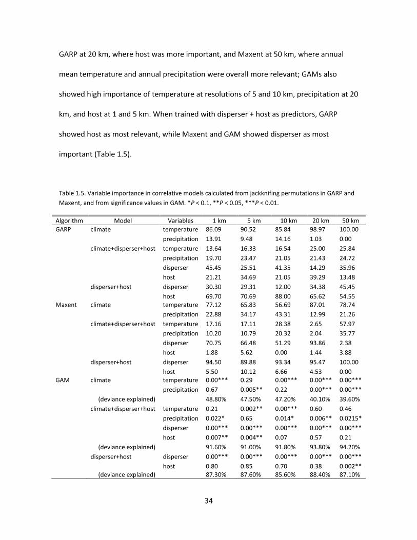
34

GARP at 20 km, where host was more important, and Maxent at 50 km, where annual

mean temperature and annual precipitation were overall more relevant; GAMs also

showed high importance of temperature at resolutions of 5 and 10 km, precipitation at 20

km, and host at 1 and 5 km. When trained with disperser + host as predictors, GARP

showed host as most relevant, while Maxent and GAM showed disperser as most

important (Table 1.5).

Table 1.5. Variable importance in correlative models calculated from jackknifing permutations in GARP and

Maxent, and from significance values in GAM. *P < 0.1, **P < 0.05, ***P < 0.01.

Algorithm Model Variables 1 km 5 km 10 km 20 km 50 km

GARP climate temperature 86.09 90.52 85.84 98.97 100.00 precipitation 13.91 9.48 14.16 1.03 0.00 climate+disperser+host temperature 13.64 16.33 16.54 25.00 25.84 precipitation 19.70 23.47 21.05 21.43 24.72 disperser 45.45 25.51 41.35 14.29 35.96 host 21.21 34.69 21.05 39.29 13.48 disperser+host disperser 30.30 29.31 12.00 34.38 45.45 host 69.70 70.69 88.00 65.62 54.55 Maxent climate temperature 77.12 65.83 56.69 87.01 78.74 precipitation 22.88 34.17 43.31 12.99 21.26 climate+disperser+host temperature 17.16 17.11 28.38 2.65 57.97 precipitation 10.20 10.79 20.32 2.04 35.77 disperser 70.75 66.48 51.29 93.86 2.38 host 1.88 5.62 0.00 1.44 3.88 disperser+host disperser 94.50 89.88 93.34 95.47 100.00 host 5.50 10.12 6.66 4.53 0.00 GAM climate temperature 0.00*** 0.29 0.00*** 0.00*** 0.00*** precipitation 0.67 0.005** 0.22 0.00*** 0.00*** (deviance explained) 48.80% 47.50% 47.20% 40.10% 39.60% climate+disperser+host temperature 0.21 0.002** 0.00*** 0.60 0.46 precipitation 0.022* 0.65 0.014* 0.006** 0.0215* disperser 0.00*** 0.00*** 0.00*** 0.00*** 0.00*** host 0.007** 0.004** 0.07 0.57 0.21 (deviance explained) 91.60% 91.00% 91.80% 93.80% 94.20% disperser+host disperser 0.00*** 0.00*** 0.00*** 0.00*** 0.00*** host 0.80 0.85 0.70 0.38 0.002** (deviance explained) 87.30% 87.60% 85.60% 88.40% 87.10%

35

Discussion

The two modeling approaches that we implemented are very different in nature (Morin

and Thuiller 2009). In the process-based model, we made explicit assumptions about the

way that the mistletoe could be dispersed and in this way “explore” the region, and

reasons behind it successfully establishing or not given the availability of hosts and abiotic

climatic conditions. On the other hand, in the correlative models, mechanisms shaping

the distribution are implicit in associations between occurrence of the species and

environmental factors. The differences and similarities between the results of the two

approaches illuminate the roles of different factors across different spatial scales (Schurr

et al. 2012). We could think of process-based models as a hypothetic-deductive approach

by which to test hypothesis, whereas correlative models are an inductive way to propose

hypotheses; the differences in results are explained by the ways in which the two

methods make use of observations.

The results from the process-based model suggest that dispersal factors are most

relevant at fine resolutions, but that they become practically irrelevant at coarser

resolutions, where climatic factors dominate, as expected under the Eltonian Noise

Hypothesis (Soberón and Nakamura 2009, Peterson et al. 2011). This result is consistent

with previous general thinking about effects of scale on the relative importance of

different factors on distributional ecology (Whittaker et al. 2001, Pearson and Dawson

2003), and also with previous results on spatial aggregation patterns of P. californicum

(Aukema 2004). This later study found mistletoe aggregation within trees and at about

1.5-2 km, and again at a distance ≥ 4 km, that was correlated with elevation. This finding

36

led the author to hypothesise that dispersal was key to the first two scales (within trees

and ~1500 m) and abiotic factors to the > 4 km scale. Although our simulations did not

include these finer resolutions, our results are consistent where comparisons were

possible. Coincident aggregation patterns have also been reported in studies of the Indian

mistletoe Taxillus tomentosus (Lemieux et al. 2011).

The fact that parameters of the extinction rate did not show significant change

across resolutions is consistent with the relative stability of scenopoetic variables across a

broad set of scales (Soberón 2007). Scenopoetic variables are related to the abiotic

fundamental niche, an adaptive feature related to physiology (James et al. 1984, Jackson

and Overpeck 2000). In this case, climate is relevant because it adjusts species’ survival

limits in each cell of the grid. Overall, what is apparently changing with scale are factors

associated with dispersal of the species, as seen in the colonization part of this model,

whereas climate is a constant determinant of the species’ range across scales. These

results support the hypotheses proposed with the BAM diagram in the conceptual

framework (Fig. 1.2).

Process-based models, which are much more time-consuming to implement than

correlative models, are nevertheless potentially very informative. After comparing the

models generated in this exercise, it is evident that incorporating colonization and

extinction processes within a metapopulation framework sheds light on the importance

that factors related to dispersal may have at finer scales for this species (Overton 1994,

1996, Aukema 2004, Lemieux et al. 2011), and that more stable factors like climate either

37

remain constant across resolutions or become more important in controlling the

distribution of the species as the resolution becomes coarser.

Using correlative methods, we were able to perceive differences in contributions

of variables as a function of changes in resolution, as other authors have shown (e.g.,

Buckley et al. 2010). However, interpretation of the roles of different variables, not being

linked to mechanisms, was not straightforward, and potentially would lead to

interpretations very different from what we observed using the process-based model

(Cabral and Schurr 2010). Araújo and Luoto (2007) used GAMs to test whether biotic

interactions played a role at macroscales for the butterfly Parnassius mnemosyne: they

found that the type of interaction (contingent on species) and methods considered played

significant roles in explaining distributions of species at coarse scales. Other studies using

correlative approaches have shown improvement in predictions of species’ distributions

when resource-related variables are incorporated (Heikkinen et al. 2007, Real et al. 2009,

Wisz et al. 2012). In our exercise, when we used correlative models, we also found that

biotic-related predictors play a role at coarse scales, but were most relevant at scales

finer than the macroscale of Araújo and Luoto (2007). These authors worked only at a

scale similar to the coarsest of our analysis (50 km); they might have detected additional

patterns if their analysis had extended to finer resolutions. Their results match ours at the

coarsest resolution if we consider both disperser and host layers as part of the mistletoe’s

biotic interactions: in our case, the disperser layer showed some explanatory power,

although not very significant, whereas, in Araújo and Luoto’s example, the host plant

distribution of the butterfly did not improve results drastically, but rather echoed climate

38

signals (Figs. 1.3 and 1.4). Although these results from correlative models suggest that

non-scenopoetic variables are important at coarse scales, the process-based model

helped us to understand interactions among predictors, and revealed contrasting

importance of factors at different resolutions.

Our analysis suggests that different combinations of environmental predictors,

whether biotic or abiotic, may affect interpretation of model predictions drastically,

offering a step towards understanding model overfitting. Addition of the disperser layer

resulted in concentration of the mistletoe’s predicted distribution in the area of highest

density of the disperser. Although model overfitting is known to complicate estimates of

species’ ecological niches (Peterson et al. 2007), in this case, it also shows how

combinations of abiotic and dispersal-related predictors restrict the area predicted as

suitable. An improvement on this exploration would be to test for significance of

explanatory power of other (less important) dispersers and perhaps different suites of

hosts in the model.

It is interesting to notice that the different modeling approaches produced

predictions with only fair to good agreement. One possible explanation for such lack of

coincidence is that the climate-only predictions agree closely with the distribution of the

disperser, which is the element of the process-based model that covers the entire extent

moving the parasite across cells in search for suitable conditions for its establishment (M;

Barve et al. 2011). However, in the metapopulation framework of the process-based

model, the disperser is just one part of the formula, and how the mistletoe reaches its

distributional limits depends on the balance between colonization and extinction.

39

Assuming that the disperser actually carries mistletoe seeds all across the study extent

and that hosts are present, our study suggests that the mistletoe is able to reach and

potentially establish in areas more distant than the known geographic range edges;

however, its populations are restricted to an area smaller than its “accessible area,”

suggesting that other factors (including climate) constrain its survival. In a more realistic

process-based modeling approach, actual seed processing times and dispersal distances

could be incorporated (e.g., Overton 1996, 1997, Liu et al. 2011).

The fact that the species is not present in the northwestern and southeastern

parts of the disperser’s range suggests that the species is responding to some

combination of biotic and abiotic factors that reduces suitability in those regions (Fig. 1.1;

see also Fig. S1.1). The two areas are consistently predicted as climatically suitable, but

densities of disperser and hosts are much lower towards these two areas, very different

from the central part of the study area, where we observed highest mistletoe

abundances; areas similar to these areas may be worth exploring in detail for sink

population dynamics. From observations during field work, the transition between

absence and presence, moving from east to west, could also be explained by a

combination of biogeographic barriers for the species and dramatic environmental

gradients, which represent limits to dispersal (although other generalist and specialist

species are present in these other regions) and successful establishment. Our

observations do not suggest interference by other species (i.e., other biotic factors, such

as competition) in this part of the range; rather, it is more likely that the species has not

been able to adapt to abiotic conditions there, preventing it from being more widespread.

40

This may explain why the species is restricted to the Sonoran Desert and parts of the

Mojave Desert, and does not occur in other, adjacent desert areas in North America, such

as California’s Central Valley, the Chihuahuan Desert, or the Valle de Tehuacán in Mexico,

that present different combinations of either hotter and wetter or colder and dryer

climates, in comparison to areas where the species is present (Dimmit 2000).

Although our exercise is realistic according to what we know about the species’

distribution and how biotic and abiotic factors operate across scales, it carries some

significant assumptions and limitations. First, the environmental predictors we used and

the way they were developed is far from ideal. We chose predictors that are likely

important to the species, but generating them and matching their resolutions was not

always possible. In particular, this concern applies to the disperser layer: it was originally

created at a spatial resolution of 461 km2 (Sauer et al. 2011), but data availability

considerations prevented us from scaling it directly to other resolutions. Scaling it to high

resolutions requires a larger density of survey routes than is actually available; as a

consequence, we used this single resolution for the first four resolutions, and generalized

it still more for the coarsest.

Other bioclimatic variables could have been chosen, such as those associated with

extremes of temperature and precipitation; however, in tests using other sets of climate

variables and the entire set of 19 bioclimatic variables of Hijmans et al. (2005), neither the

process-based model nor the correlative approach appeared to benefit from such

additional information (data not shown). To check this point more thoroughly, we tested

the performance and geographic predictions of correlative models with two other

41

environmental layers that were calculated using daily weather stations information for a

period of 20 years: number of continuous days of freezing temperatures and number of

continuous rainless days. However, these models did not produce results markedly better

than annual mean temperature and annual precipitation visually, nor did models increase

in performance, which suggests that different trends would not result in either the model

prediction or in model performance.

For the process-based model, it would be possible to create and explore other

colonization and extinction functions. In particular, the extinction function used was a

simple exponential of the difference between the estimated optimal niche and the

environments of a given cell: clearly, more complex may prove more appropriate

(Martínez-Meyer et al. 2013). However, based on extensive initial exploration and

simulations (not shown), in which our basic results were supported, it is not likely that

major differences and conclusions from our current findings would emerge.

Other types of information could be incorporated in new models, as well as in

experiments that could analyze details of mistletoe population dynamics in different parts

of the range. For example, numbers of viable seeds dispersed by Phainopepla nitens and

other bird species may indicate regions with unfavorable niche conditions and sink

population dynamics, or perhaps even other physiological mechanisms of host-parasite

recognition. Other studies of such dynamics in P. californicum have been carried out at

much finer resolutions than ours, and are very illuminating when compared with our

macro-geographic approximations (e.g., Overton 1994, 1996, Aukema and Martínez del

Rio 2002, Liu et al. 2011). From an ecological point of view, for example, these analyses

42

would allow exploring whether abundance, genetic variation, population differentiation,

or gene flow vary as functions of centrality within the geographic range (Thuiller et al.

2010, Torres et al. 2012, Martínez-Meyer et al. 2013) or the ecological niche of the

species, thus presenting different opportunities for local optima and associated

adaptation (VanDerWal et al. 2009, Martínez-Meyer et al. 2013).

Acknowledgments

We are thankful to Luis A. Sánchez-González, Gerardo Cendejas, Fran Recinas, and

Rebecca Crosthwait for invaluable support during field work. We are indebted to several

institutions and herbaria where we stored specimen material: Centro Interdisciplinario de

Investigaciones para el Desarrollo Integral Regional, Durango (Socorro González), Instituto

de Biología, UNAM (Hilda Flores), Universidad Autónoma de Baja California, Ensenada

(José Delgadillo), and San Diego Natural History Museum (Jon Rebman). We thank Luis

Eguiarte and Mark Olson for help with logistics, and the warm hospitality of the families

of Alberto Búrquez, Pablo Lazo, Socorro González, Gerardo Cendejas, and Rebecca

Crosthwait made field work much easier. Initial discussions about this work with Carlos

Martínez del Río and statistical guidance from Exequiel Ezcurra were crucial. We also

thank A. Townsend Peterson for insightful comments on this work and Narayani Barve for

help with weather values interpolation. Conversations with Richard Felger and Mark

Robbins were important to clarify points on climatic limiting factors and dispersal of the

species. We thank the curators and staff of the following herbaria for providing access to

their digital data: ARIZ, ASC, ASU, BCMEX, BNHM, CANB, COCHISE, DES, GBIF, GCNP, IZTA,

43

KANU, LL, MABA, MO, NMBCC, NY, RM, SNM, TEX, UCR, UNM, USON, UTC, UVSC, XAL.

Comments from David M. Watson and two anonymous reviewers were highly valuable in

improving the quality and clarity of the analyses. A Tinker Award from the Department of

Latin American Studies and Biodiversity Institute Panorama small grant award (Bunker

Fund), University of Kansas, supported part of the collecting trip. C.P.M.’s work was

supported by Microsoft Research grant 47780. A.L.-N. received a graduate fellowship

support from the Consejo Nacional de Ciencia y Tecnología (189216).

44

Chapter 2

Range-wide ecological niche comparisons of

parasite, hosts and dispersers in a vector-borne

plant parasite system2

2 Lira-Noriega A, Peterson AT (In press) Range-wide ecological niche comparisons of parasite, hosts and dispersers in a vector-borne plant parasite system. Journal of Biogeography. Doi: 10.1111/jbi.12302

45

Abstract

We aim to test whether the distribution of the mistletoe Phoradendron californicum is

mediated by host distributions (host niche hypothesis, HNH), or by factors such as the

mistletoe’s autecology (parasite niche hypothesis, PNH) or that of its vectors (vector niche

hypothesis, VNH). Our null hypothesis is that the ecological niche of the mistletoe will not

be distinct from that of its hosts or vectors; alternatively, mistletoe infections might

appear in hosts only in regions where host distributions overlap suitable conditions for

the parasite. We used ecological niche modelling approaches to summarize suitable

environmental conditions for hosts infected and uninfected with mistletoes, as well as for

avian dispersers during winter and throughout the year. We compared ecological niches

among pairs of species using background similarity tests in relation to the climatic

conditions available and accessible to each species. Results show that niche comparisons

supported all PNH expectations, but none of the predictions of HNH or VNH. These

findings suggest that hosts and dispersers of mistletoes generally have distinct ecological

niches; mistletoe infections occur in non-random environmental subsets of host and

disperser ecological niches; mistletoe infections in different hosts, however, occur under

similar climatic conditions. Hence, in this system, the parasite has a rather strictly

circumscribed ecological niche, and host species become infected with mistletoe only

where they overlap its suitable areas.

46

Introduction

Parasites are abundant in the natural world. Because their life cycles often involve

interactions among multiple species, parasites offer great study opportunities to

understand degrees of specificity and transmission capacities in the context of species’

ecological and evolutionary dynamics (Morand and Krasnov, 2010). These phenomena are

important in illuminating the relationships of parasites with hosts, the ranges of hosts

that parasite species can infect and mechanisms of infection. In general, two interesting

questions arise: to what extent are animal and plant populations affected by parasitism

and disease (Begon et al., 2006), and under what conditions do infections occur?

Recent studies of the ecology of mistletoes have opened opportunities to

understand plant parasitism and species’ distributions at multiple spatial scales.

Mistletoes are vector-borne parasites that play dual roles in biological communities: as

parasites of host plants and as mutualists with birds (Martínez del Rio et al., 1996;

Aukema, 2003). Birds obtain nutrients, energy and water from mistletoes, whereas

mistletoes benefit from seed dispersal to safe establishment sites (Reid, 1991). The desert

mistletoe, Phoradendron californicum Nutt. (Viscaceae; henceforth simply ‘mistletoe’), is

a hemiparasitic plant distributed in parts of the Sonoran and Mojave deserts (Kuijt, 2003)

that is parasitic almost exclusively on leguminous trees. Host species include Acacia

constricta Benth., Acacia greggii A. Gray, Cercidium floridum Benth. ex A. Gray, Cercidium

microphyllum (Torr.) Rose and I.M. Johnst., Olneya tesota A. Gray, Prosopis glandulosa

Torr. and Prosopis velutina Wooton, and less commonly Larrea tridentata (Sessé and

Moc. ex DC.) Coville (Zygophyllaceae), Celtis pallida Torr. (Cannabaceae), Condalia

47

warnockii M.C. Johnst. (Rhamnaceae) and Tamarix ramosissima Ledeb. (Tamaricaceae)

(Haigh, 1996).

The mistletoe’s distribution is shaped at least in part by the activities of avian

seed-dispersers (Larson, 1996; Aukema, 2001). Differences in fruit removal and dispersal

distances result from different combinations of frugivore abundances and plant

aggregation, two large-scale processes that can control and structure small-scale

neighbourhood patterns (Carlo and Morales, 2008). Particularly important are the roles of

specialist and generalist mistletoe fruit consumers in dispersing seeds closer to existing

infections or beyond them, respectively (Aukema and Martínez del Rio, 2002a;

Rawsthorne et al., 2012).

Because mistletoe fruits are among the few berries available in these North

American deserts during winter, they represent an important food source for birds when

other food is scarce (Cowles, 1936). The most common birds feeding on Phoradendron

californicum berries include Phainopepla nitens (Swainson, 1838) (Ptilogonatidae),

Melanerpes uropygialis (S.F. Baird, 1854) (Picidae), Mimus polyglottos (Linnaeus, 1758)

(Mimidae) and Toxostoma curvirostre (Swainson, 1827) (Mimidae), and less commonly

Bombycilla cedrorum (Vieillot, 1808) (Bombycillidae), Campylorhynchus brunneicapillus

(Lafresnaye, 1835) (Troglodytidae), Carpodacus mexicanus (Statius Müller, 1776)

(Fringillidae), Callipepla gambelii (Gambel, 1843) (Odontophoridae), Myadestes

townsendi (Audubon, 1838) (Turdidae), Sialia currucoides (Bechstein, 1798) (Turdidae),

Sialia mexicana (Swainson, 1832) (Turdidae), Sialia sialis (Linnaeus, 1758) (Turdidae),

Turdus migratorius (Linnaeus, 1766) (Turdidae), Oreoscoptes montanus (J.K. Townsend,

48

1837) (Mimidae), Toxostoma crissale (Henry, 1858) (Mimidae) and Zonotrichia leucophrys

(J.R. Forster, 1772) (Emberizidae) (Larson, 1996). Of these species, P. nitens is considered

the primary and most efficient mistletoe seed disperser (Larson, 1996). Indeed,

phainopeplas have a digestive system specialized to be able to process hundreds of

mistletoe berries per day (Walsberg, 1975), and their breeding season in the desert

coincides with fruiting periods of mistletoes (Chu and Walsberg, 1999).

Mistletoe distribution and prevalence have been explained more generally in

terms of interactions among local and regional determinants, although the precise

mechanisms and differential influences of biotic and abiotic factors remain largely

unknown (Watson, 2009; Kavanagh and Burns, 2012; Lira-Noriega et al., 2013). Although

most studies have focused at local scales, some recent studies have examined influences

of factors at multiple spatial scales (e.g. Rist et al., 2011; Kavanagh and Burns, 2012; Lira-

Noriega et al., 2013). Nonetheless, variation in host quality and specificity (Watson, 2009)

and the effectiveness of seed dispersal by different vectors (Montaño-Centellas, 2013)

remain important factors. To date, however, no study has examined ecological and

geographical relationships among mistletoes, hosts and seed dispersers in the context of

climatic conditions as range-wide determinants; such an approach would complement

the current knowledge of mistletoe ecology.

In a study of range-wide determinants of plague (Yersinia pestis) distribution in

North America, Maher et al. (2010) analysed niche overlap among infected and

uninfected hosts to test whether the distribution of plague in North America is mediated

by the ecological niches of mammal hosts or rather by those of the vectors or the

49

pathogen per se (Fig. 2.1). Here, we test whether the mistletoe’s distribution is mediated

by ecological niches of its hosts (‘host niche hypothesis’), or rather by its own ecology

(‘parasite niche hypothesis’) or that of its multiple dispersers (‘vector niche hypothesis’).

The null expectation is that mistletoe infections occur under environmental

circumstances not distinguishable from the ecological niches of its hosts or dispersers;

alternatively, mistletoe infections might appear only where host distributions overlap

suitable areas for the parasite. To test these hypotheses, we used an ecological niche

modelling approach to estimate ecological niches, and then compared niches of pairs of

species, specifically assessing the amounts of niche overlap in relation to the overlap of

environmental conditions accessible and available to each species (Warren et al., 2008).

50

Figure 2.1 Conceptual diagram of relationships between mistletoe occurrences, host and vector occurrences, and environmental variation (a) under the host niche hypothesis (HNH) and vector niche hypothesis (VNH), and (b) under the parasite niche hypothesis (PNH). Occurrence of the parasite with respect to two dimensions of the scenopoetic fundamental niche (E1 and E2) is shown as a thick black line. Grey polygons in the upper panel show a mosaic of host or vector niches; in the lower panel, the grey polygon shows the parasite’s niche and dashed outlines show the niches of hosts and/or vectors. (Figure modified from Maher et al., 2010.)

Materials and Methods

Input data

We collected occurrence data based on herbarium voucher specimens for each of the

eight most common mistletoe host species across their entire range from the Global

Biodiversity Information Facility (http://www.gbif.org/) and the Southwest Environmental

Information Network (http://swbiodiversity.org/portal/index.php). These tree species all

51

occur in the Sonoran Desert, some extending as far as the mid-western United States or

central Mexico. The numbers of unique occurrences available for these species were:

Acacia constricta, 326; Acacia greggii, 946; Cercidium floridum, 345; C. microphyllum, 694;

Larrea tridentata, 616; Olneya tesota, 631; Prosopis glandulosa, 914; and Prosopis

velutina, 1169. We also assembled information on mistletoe occurrences associated with

each host species from the same online databases, as well as from A.L.-N.’s field

collections across the geographical range of the species in 2010 and 2012 (Lira-Noriega et

al., 2013). The numbers of unique occurrences of infected hosts were: A. constricta, 8; A.

greggii, 131; C. floridum, 13; C. microphyllum, 23; L. tridentata, 8; O. tesota, 30; P.

glandulosa, 37; and P. velutina, 45. Special attention was paid to obtaining adequate

numbers of occurrences well spread across the species’ range. To corroborate that the

scientific names we used provided accurate numbers and distributions of records, we

conducted further searches using synonyms and subspecies, but this step did not

substantially alter the numbers or distributions of occurrences.

A list of 10 potential bird dispersers for this study was derived from our own field

observations and those of knowledgeable ornithologists (A.L.-N.; A.T.P.; Mark Robbins,

University of Kansas, pers. comm.). This list overlaps with what has been reported in the

literature (Larson, 1996). Distributional data for potential bird dispersers were drawn

from eBird (http://ebird.org/content/ebird/), and numbers of unique occurrences year-

round and for winter (December–February) were Mimus polyglottos (year, 247,566;

winter, 91,717), Myadestes townsendi (22,600; 7156), Phainopepla nitens (15,487; 5491),

Toxostoma curvirostre (6666; 1944), Sialia currucoides (23,601; 5944), S. mexicana

52

(39,788; 14,036), S. sialis (72,734; 62,923), Bombycilla cedrorum (171,102; 47,225),

Melanerpes uropygialis (11,401; 4498) and Turdus migratorius (300,925; 91,355).

To characterize environmental variation across the region, we used climatic

summaries from the WorldClim data archive (Hijmans et al., 2005;

http://www.worldclim.org/) at a spatial resolution of 2.5'. To avoid fitting models in

environmental spaces with too many dimensions, we used principal components analysis

(PCA) on standardized variables with the ‘prcomp’ function in R (R Development Core

Team 2013) among 15 ‘bioclimatic’ variables (annual mean temperature, mean diurnal

temperature range, isothermality, temperature seasonality, maximum temperature of

the warmest month, minimum temperature of the coldest month, annual temperature

range, mean temperature of the warmest and coldest quarters, annual precipitation,

precipitation of the wettest and driest months, precipitation seasonality and precipitation

of the wettest and driest quarters). We then reduced dimensionality to the first six

principal components, which accounted for > 95% of overall variance in the

environmental variables. Principal components were generated for the geographical

extent that encompasses all of the species’ background areas, but models were calibrated

across each species’ individual background area (see below).

Niche modelling

Ecological niche models must be calibrated and compared across regions relevant to the

species. Model calibration should thus be restricted to the accessible area: the set of sites

that the species is likely to have ‘sampled’ over a relevant period of time (Barve et al.,

2011). Here, we designed model calibration regions for each species. As a simple means

53

of estimating the accessible area, we assigned this region to cover the ecoregions (Olson

et al., 2001) in which species’ occurrence points fell, plus a 200-km buffer around them.

This region is a simple hypothesis of the areas accessible to each species that was used in

both model calibration and niche-overlap comparisons using background similarity tests

(see below).

The occurrences used to characterize ecological niches were selected as follows.

To model each host species’ ecological niche, we selected sets of 100 occurrences at

random, but we used all occurrences for mistletoe infections of host trees. For dispersers,

we selected three sets of 100 occurrences at random per species for both year-round and

winter distributions. Each host species thus had a single niche estimate, whereas each

bird had six. Two additional niche estimates were included in niche similarity comparisons

with potential dispersers (see below): an overall ‘niche’ of all host species was estimated

using three sets of 100 points selected at random from the set of non-infected host

occurrences, and the overall mistletoe niche was estimated using all mistletoe

occurrences regardless of host.

We used MAXENT (3.3.3.e; Phillips et al., 2006) to calibrate the niche models. We

used 10 bootstrap replications and a threshold of E = 10% of calibration occurrence data

over the median estimate to convert the initial model outputs to binary predictions

(Peterson et al., 2011). The remaining parameters were given their default values. The

final niche estimates for bird species corresponded to regions where all three thresholded

estimates coincided, thus providing a conservative estimate of suitable environmental

conditions.

54

The performance of the binary predictions was evaluated using a one-tailed

cumulative binomial test to calculate the probability of obtaining that level of sensitivity

by chance alone. We ran this test with 100 independent test points in cases in which

numbers of records were sufficient to set aside 100 independent test points (29 models);

for species with 14–100 records, we evaluated models by calibrating models with 50% of

occurrences and applying the binomial test to the remaining 50% (6 models). The overall

mistletoe niche binary prediction was assessed with 100 independent test points from

Phoradendron californicum occurrences that were available in the databases but that did

not specify a host species. Binary predictions from species with fewer than 14

occurrences (three models) were evaluated using a jack-knifing approach (Pearson et al.,

2007), which requires a model to be run for each subset of n − 1 occurrences, and model

performance to be tested over the removed coordinate; these probabilities were

calculated using PVALUECOMPUTE (Pearson et al., 2007).

Niche similarity estimates

Niche similarity among species was estimated using Schoener’s D and Hellinger’s I indices

via the ‘niche.overlap’ function in PHYLOCLIM (Heibl and Calenge, 2013), following the

background similarity test proposed by Warren et al. (2008). This test assesses

environmental differences between known occurrences of two species but – critically –

considers the ‘background’, which we interpret as equivalent to the accessible area for

each species (Barve et al., 2011). The test works by comparing observed overlap values

between geographical manifestations of two niches to a distribution generated from

comparing the niche models based on the observed distribution of one species to niche

55

models based on the background of the other; background occurrence points are drawn

at random from the accessible area, in numbers matching the sample size available for

the species (Warren et al., 2008).

These comparisons were carried out between all combinations of mistletoe-

infected and non-infected hosts, and between mistletoe distributions and those of

potential bird dispersers, year-round and only in winter (also including overall host and

mistletoe distributions). The first set of comparisons was made considering the

background of each host species for niche models based on occurrences of infected and

non-infected hosts, and also only for the area where each host’s accessible area

intersects the mistletoe’s accessible area. This last selection of background areas created

a more strict and conservative comparison. The second set of comparisons was made

considering the backgrounds of each bird species, overall hosts, and the mistletoe.

Background similarity distributions were estimated using 100 replicate models

calibrated and thresholded in MAXENT exactly as for the observed models, except that

occurrences were collections of random points equivalent in number to those used to

construct ‘observed’ niche models (see Warren et al., 2008). All models were thresholded

(see above) prior to the calculation of similarity indices, which reduces the effects of

overfitting (Peterson et al., 2007). We also constrained models to the same geographical

extent by merging them with a zero-value raster of the same spatial resolution as the

environmental layers. In comparing niche models, we sought to identify situations in

which niches were significantly different, i.e. when niche overlap between a pair of

species is less similar than expected at random. Hence, our null hypothesis was that the

56

two species were similar, which we rejected when the observed I and D values from niche

models on the basis of known occurrence points fell in the lowest 5% of background

similarity values.

Results

Overall host and mistletoe-infected niche comparisons

The mistletoe occurrences were all recorded in the Sonoran Desert and parts of the

Mojave Desert. They were unevenly distributed across the region, showing more or less

restricted patterns depending on the host species they were parasitizing (Fig. 2.2).

Considerable variation in numbers of mistletoe-positive occurrences was observed,

depending on host. Hence, this system offered rich regional and environmental variation,

and thereby an excellent basis for the hypothesis-testing that is the focus of this study.

57

Figure 2.2 Comparison of host niche models and mistletoe-infected-host niche models. In each map, the host’s overall suitable area is in black, the mistletoe-infected portion of the host’s distribution in transparent light grey, host occurrence points are shown as white dots, and mistletoe-infected host occurrence points as white triangles containing black dots. North America Albers equal-area conic projection.

58

All niche models performed significantly better than random expectations in all

model evaluation exercises (P < 0.001; Appendix 2.1). The modelled niches based on

mistletoe-infected hosts differed markedly from those based on all host occurrences (Fig.

2.2), and none of the geographical projections of mistletoe-infected hosts covered the

entirety of any of the host niche estimates (Fig. 2.2). Examples of background similarity

tests between the overall mistletoe niche and dispersers are shown in Fig. 2.3.

Figure 2.3 Two example background similarity tests showing amounts of niche overlap of the mistletoe overall distribution with specialist (Phainopepla nitens) and generalist (Melanerpes uropygialis) bird dispersers. The histogram shows the distribution of Hellinger’s I from the 100 random-draw models; the observed overlap value of the index for each pair of species is shown as a dashed line. The maps show the two niche-model-based predictions of the mistletoe and each bird species according to winter occurrences. North America Albers equal-area conic projection.

Niche dissimilarity between host niche distributions was observed generally

between host species with large geographical ranges (Acacia greggii, Prosopis glandulosa

and Larrea tridentata) and backgrounds of more geographically restricted species

59

(Cercidium floridum, C. microphyllum, Olneya tesota and Prosopis velutina). This effect

was observed in 13 of 56 comparisons (P < 0.05; Fig. 2.4). In contrast, no mistletoe-

infected hosts showed dissimilarity against the background of any host species (P < 0.05;

Fig. 2.4).

Figure 2.4 Results of background similarity tests from comparisons of host niche models and mistletoe-infected-host niche models. Rows represent point occurrence data and columns show species’ background areas in the similarity test. Results based on the two similarity indices were the same. Grey indicates that similarity could not be rejected (P > 0.05); black indicates that similarity was rejected (P < 0.05).

Disperser niche comparisons

Most disperser ranges covered large areas of North America, the only exceptions being

species restricted to the Sonoran Desert (e.g. Melanerpes uropygialis and Phainopepla

nitens). Niche comparisons among the 10 bird species showed frequent niche

60

dissimilarities in tests of year-round and winter distributions (P < 0.05; Fig. 2.5); the

similarity was less, however, when niches were based on occurrences from the entire

year. Two species in particular tended towards higher niche overlap in winter compared

to year-round distributions: Sialia currucoides and Turdus migratorius (P < 0.05; Fig. 2.5).

Most cases of niche dissimilarity were observed in comparisons involving Myadestes

townsendi, S. sialis and T. migratorius; in contrast, Melanerpes uropygialis, Mimus

polyglottos, P. nitens, S. mexicana and Toxostoma curvirostre showed similarity with

other species (P < 0.05; Fig. 2.5).

61

Figure 2.5 Results of background similarity tests in comparisons of bird disperser niche models for year-round and winter distributions and overall mistletoe and host niche models. Rows represent point occurrence data and columns show background areas in similarity tests. Results based on the two similarity indices were the same. Grey indicates that similarity could not be rejected (P > 0.05); black indicates that similarity was rejected (P < 0.05).

Niche comparisons between overall hosts and mistletoe against dispersers’

backgrounds showed greater niche similarity than comparisons in the other direction (P <

0.05; Fig. 2.5). Hosts were similar overall to the year-round niches of Bombycilla

cedrorum, Turdus migratorius, M. polyglottos, Myadestes townsendi, P. nitens, S.

currucoides, S. mexicana and Toxostoma curvirostre, and to winter niches of the same

62

species (except S. mexicana). The mistletoe’s niche was similar to year-round and winter

niches of all 10 potential dispersers except S. sialis.

Comparing niches of dispersers to the overall host background, only Melanerpes

uropygialis, Mimus polyglottos, P. nitens, S. currucoides, S. mexicana and T. curvirostre

were similar for year-round and winter niche predictions. Compared to the mistletoe

background, the dispersers Melanerpes uropygialis, Mimus polyglottos, P. nitens and S.

sialis were similar in year-round niche predictions (see Fig. 2.3 for an example), and these

same species plus B. cedrorum and T. curvirostre were similar in winter niche predictions.

Discussion

Our analyses showed that: (1) hosts and dispersers of mistletoe have distinct individual

ecological niches; (2) mistletoe infections occur in non-random subsets of the niche of

each host; and (3) mistletoe infections in different hosts occur under similar niche

conditions. Dispersers showed different amounts of niche overlap between year-round

and winter, but only generalist species and one mistletoe specialist (P. nitens) were

consistently associated with the mistletoe’s and hosts’ niches. These results support the

expectation of PNH, but none of the predictions of HNH or VNH. In particular, PNH

anticipates significant non-similarity between hosts in general, but similarity among hosts

when infected with mistletoe, leading to the conclusion that host species get infected

with mistletoe only where they range into suitable and accessible areas for the mistletoe.

Another possibility is that a single host may drive the geographical distribution of

mistletoe, such that ecological niche characteristics of that host would be similar to those

63

of mistletoe infections in other host taxa. However, of the 49 pairwise comparisons of

mistletoe-infected host niche models to hosts’ overall backgrounds, none rejected

similarity (Fig. 2.4), suggesting that mistletoe infections are restricted to suitable portions

of the mistletoe’s background. This pattern thus shows a strong association of mistletoe

to an important functional group of plants, but only under particular climatic conditions

of these North American deserts.

In a study of spatial distribution and host use across 65 mistletoe species in

Australia, Kavanagh and Burns (2012) found diversity to be unrelated to productivity, but

that host ranges (i.e. number of infected host species) were broader in areas with more

potential host species. From this perspective, it is plausible that the association of

Phoradendron californicum with legumes evolved in this semi-arid region because of its

high legume diversity, offering many potential hosts (Dimmitt, 2000; Garcillán and

Ezcurra, 2003). According to the PNH, however, hosts would get infected only in areas

climatically suitable for the parasite. Our results apparently also follow what a recent

network analysis described as a non-nested and modular interaction pattern (Genini et

al., 2012), in which each of four mistletoe species from the Brazilian Pantanal

(Psittacanthus cordata, Psittacanthus calyculatus, Phthirusa abdita and Phoradendron sp.)

interacted with a particular set of hosts, with low host specificity, but with hosts highly

susceptible to mistletoe infections. That pattern is also consistent with the PNH, in which

similarity among hosts appears only in sites at which the mistletoe can occur.

Attributes of hosts and dispersers, as well as other mechanisms at multiple spatial

and temporal scales, are important to understanding the mistletoe’s distribution. As

64

proposed in the ‘host-quality hypothesis’ (Watson, 2009), variation in host quality may

account for non-random occurrence patterns of parasitic plants: parasites are expected to

establish and survive on higher-quality hosts. Host quality for mistletoes often depends

on tree height and architecture, bark texture, age and accessibility to water or drainage

sites, and host species (Norton et al., 1997; Lei, 1999; Norton and Smith, 1999; Aukema

and Martínez del Rio, 2002b; Callaway et al., 2002; Marquardt and Pennings, 2010).

Examples of differential responses to host quality in P. californicum include birds’ general

preference for taller trees with larger numbers of mistletoe plants – causing concentrated

intra-host infections (Aukema and Martínez del Rio, 2002a,b) – and the responses of birds

to mistletoe prevalence, causing disproportionate seed deposition patterns (Overton,

1996; Aukema, 2004).

Because host races (i.e. a partly reproductively isolated population of a parasite

species) and host specialization occur in P. californicum (Glazner et al., 1988; Overton,

1997) and other mistletoe species (Clay et al., 1985; Nickrent and Stell, 1990; Jerome and

Ford, 2002), it is possible to find a non-random distribution of mistletoe depending on the

mistletoe’s differential affinity for different host genera. Host specialization in P.

californicum may evolve more frequently in host-depauperate areas (Kavanagh and

Burns, 2012) and in areas of high host prevalence (Overton, 1997), a pattern expected

from the numbers and distribution of infections in this study. Several questions remain

regarding susceptibility to mistletoe parasitism and related to immunity, abundance and

changes in host quality owing to previous infection (Watson, 2009). Phylogenetic analyses

may be important in defining the relationships between the densely connected (but non-

65

overlapping) subsets of host species within a mistletoe’s network (Genini et al., 2012),

and analyses of phylogeographical and genetic structure could improve the

understanding of consequences of seed-dispersal patterns, population evolution and

host-race formation (Amico and Nickrent, 2009; Stanton et al., 2009; Zuber and Widmer,

2009; Lira-Noriega et al., unpubl. data).

The distribution and ecology of vector species is a determinant of mistletoe

distribution and aggregation patterns at multiple spatial scales (Larson, 1996; Overton,

1996; Aukema and Martínez del Rio, 2002a,b; Aukema, 2004; Rist et al., 2011; Lira-

Noriega et al., 2013). In our analyses, overall host and mistletoe niches showed similarity

with nine species of potential dispersers in year-round and winter distributions. However,

pairwise comparisons of potential dispersers and mistletoe backgrounds showed niche

similarity with only six species (Fig. 2.5). The fact that more bird species showed niche

similarity against the mistletoe background in winter comparisons coincides with the fact

that these species concentrate in this desert region when the mistletoe is a food

resource. Genini et al. (2012) hypothesized that the modularity of infection in four

mistletoe species from the Brazilian Pantanal derives from different seed dispersal

systems, such that Psittacanthus species have many bird dispersers, whereas their

Phoradendron species are dispersed by specialists.

The extent to which other bird species contribute meaningfully to mistletoe

dispersal is less certain. This role depends in part on their distributional and migration

dynamics through the year, but probably most importantly on their specificity on

mistletoe and the time they spend on hosts after eating mistletoe fruits (Larson, 1996;

66

Aukema and Martínez del Rio, 2002a). Year-round residents are typically characterized by

territoriality with shorter movements, whereas seasonal migrants could be responsible

for longer-distance dispersal events. Even though potential colonization could extend

beyond the known distributional limits of the mistletoe, successful establishment events

only occur if the right combinations of hosts and climate are also met (Lira-Noriega et al.,

2013). Differential vector roles in shaping the spatial structure of mistletoe populations

have also been documented in the Patagonian mistletoe Tristerix corymbosus (García et

al., 2009; Amico et al., 2011). While interesting, disentangling the roles of different

vectors would require analyses beyond the scope of that presented here.

Other biotic interactions may also limit the mistletoe’s distribution, such as roles

of pollinators and vertebrate and invertebrate herbivores. Although little is known about

which other species interact with P. californicum, it is possible that lepidopterans,

weevils, coreid bugs and homopterans, feed on its branches and seeds, as in the related

Phoradendron tomentosum when parasitizing Prosopis glandulosa (Whittaker, 1984).

Several rodents, deer, bighorn sheep, cattle and goats are also known to feed on

mistletoes. The spatial variation of these interactions could be studied and added as new

hypotheses to test in this system. Nonetheless, we anticipate that dispersers and hosts

will prove the most significant species in defining the mistletoe’s distribution.

From the perspective of the mistletoe and the community of species with which it

interacts, this study allowed us to corroborate, and to some extent generalize, the

ecological dynamics and patterns of association with hosts and dispersers known from

several studies at local scales and from our own observations in the field. This study offers

67

a broad-scale view of mistletoe infections, with hypotheses regarding conditions under

which they occur (Wisz et al., 2013), and reinforces the idea that mistletoes should

continue to be considered a valuable epidemiological system to understand infection

patterns in vector-borne diseases and parasite–host interactions (Aukema, 2003;

Mathiasen et al., 2008). This general approach could be easily applied to other systems of

parasitism and disease.

Acknowledgements

We thank Sean Maher for guidance on niche overlap estimates, Mark Robbins for advice

on potential mistletoe bird dispersers, Richard Felger for help with species identifications

and valuable comments on background areas, and Ben Wilder for valuable comments on

the manuscript. Comments from three referees and the editors helped improve the

manuscript. Collecting trips were supported by a Young Researchers Award from the

Global Biodiversity Information Facility (GBIF), a Tinker Award from the University of

Kansas Center of Latin American Studies, and a University of Kansas Biodiversity Institute

Panorama small grant award (Bunker Fund). A.L.-N. received scholarship support from

Consejo Nacional de Ciencia y Tecnología, Mexico (189216).

68

Chapter 3

Relationship of genetic diversity and niche

centrality: A survey and analysis3

3 Lira-Noriega A, Manthey JD (2014) Relationship of genetic diversity and niche centrality: A survey and analysis. Evolution 68: 1082-1093. Doi:10.1111/evo.12343.

69

Abstract

The distribution of genetic diversity within and among populations in relation to species’

geographic ranges is important to understanding processes of evolution, speciation, and

biogeography. One hypothesis predicts that natural populations at geographic range

margins will have lower genetic diversity relative to those located centrally in species’

distributions owing to a link between geographic and environmental marginality;

alternatively, genetic variation may be unrelated with geographic marginality via

decoupling of geographic and environmental marginality. We investigate the predictivity

of geographic patterns of genetic variation based on geographic and environmental

marginality using published genetic diversity data for 40 species (insects, plants, birds,

mammals, worms). Only about half of species showed positive relationships between

geographic and environmental marginality. Three analyses (sign test, multiple linear

regression, and meta-analysis of correlation effect sizes) showed a negative relationship

between genetic diversity and distance to environmental niche centroid, but no

consistent relationship of genetic diversity with distance to geographic range center.

Introduction

The study of species’ geographic distributions has been approached from many different

perspectives in ecology, evolutionary biology, biogeography, and macroecology (Udvardy

1969; Rapoport 1982; Brown et al. 1996; Gaston 2003; Holt and Keitt 2005). Particularly

important are geographic range edges, because they represent frontiers where

populations interact with marginal environmental conditions, to which they may or may

70

not adapt (Holt 2003; Bridle and Vines 2007; Kawecki 2008; Sexton et al. 2009; Paul et al.

2011).

Along distributional limits, populations are often sparse, fragmented, and prone to

local extinction (Gaston 2003); they may represent demographic sinks maintained by

immigration from higher-quality core habitats, which makes them demographically and

genetically dependent on other populations (Pulliam 1988). Peripheral sites may also

receive gene flow that can counteract local selection pressures and local adaptation

(Kawecki 2008). As a consequence, these populations may be more prone to loss of

genetic diversity (Kawecki 2008; Keller et al. 2010).

This pattern has been illustrated as a hypothesized relationship between local

abundance and geographic centrality, in which abundances would be higher in central

populations versus peripheral ones (e.g., Brown 1984; Brussard 1984; Vucetich and Waite

2003). This idea is called the abundant-center hypothesis (Hengeveld and Haeck 1982).

However, exceptions to the pattern have been reported frequently (e.g., Sagarin and

Gaines 2002; Gaston 2003; Martínez-Meyer et al. 2013). Although higher genetic diversity

may be expected at range centers than at range edges, empirical patterns have been

mixed (Eckert et al. 2008; Kawecki 2008; Moeller et al. 2011).

The distance to the center of the geographic distribution per se should perhaps

not be expected to cause abundance or genetic variability differences. Demographic

processes may relate more directly to the quality of local conditions, as expressed by the

fundamental ecological niche of the species (Hutchinson 1957, 1978; Pulliam 2000;

Soberón 2010; Martínez-Meyer et al. 2013). The fundamental niche is the set of

71

environmental conditions under which the species shows positive population growth

rates without immigration; outside of those conditions, the species shows zero or

negative population growth. Under this alternative framework, populations under

conditions closer to the core of the fundamental ecological niche would achieve higher

growth rates or greater stability than those far from the optimum conditions (VanDerWal

et al. 2009). Of special note is that environmentally ‘central’ conditions frequently are not

located at the center of the geographic range. Therefore, an important question arises:

are demographic and genetic effects of peripherality manifested more consistently in

geographic or environmental spaces?

Under one hypothesis (H0 in Fig. 3.1), geographic marginality and ecological

marginality are positively linked, creating a relationship between geographic marginality

and population characteristics (e.g., local abundance or genetic diversity). Alternatively,

geographic marginality and ecological marginality may be decoupled (HA in Fig. 3.1),

leading to a lack of a relationship between geographic marginality and population

characteristics. The key assumption behind these hypotheses is that environmental

marginality causes adverse population effects. Here, environmental marginality may lead

to small population sizes (i.e., an environmental version of the abundant-center

hypothesis), which in turn causes population genetic processes to reduce genetic

diversity. Increased genetic drift in small populations, source-sink dynamics of

unsustainable populations, or strong selection in marginal environments could all

contribute to environmental marginality reducing genetic diversity within a species.

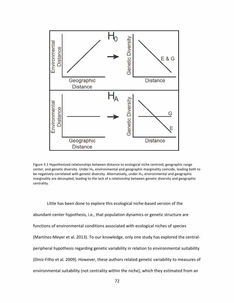
72

Figure 3.1 Hypothesized relationships between distance to ecological niche centroid, geographic range center, and genetic diversity. Under H0, environmental and geographic marginality coincide, leading both to be negatively correlated with genetic diversity. Alternatively, under HA, environmental and geographic marginality are decoupled, leading to the lack of a relationship between genetic diversity and geographic centrality.

Little has been done to explore this ecological niche-based version of the

abundant-center hypothesis, i.e., that population dynamics or genetic structure are

functions of environmental conditions associated with ecological niches of species

(Martínez-Meyer et al. 2013). To our knowledge, only one study has explored the central-

peripheral hypothesis regarding genetic variability in relation to environmental suitability

(Diniz-Filho et al. 2009). However, these authors related genetic variability to measures of

environmental suitability (not centrality within the niche), which they estimated from an

73

average of ecological niche model suitability scores from multiple niche modeling

algorithms; they found no clear relationships.

The above situation suggests that reassessment of the traditional geographic

abundant-center hypothesis (Sagarin and Gaines 2002; Gaston 2003; Garner et al. 2004;

Eckert et al. 2008) in terms of ecological niches is necessary. Particularly important to this

point are differences between environmental conditions near the core of the geographic

distribution versus those at its periphery, because these contrasting environments are

where key components of selection, adaptation, and evolution are—or are not—taking

place (Bridle and Vines 2007; Kawecki 2008; Bozinovic et al. 2011). Soberón and Miller

(submitted) extended models originally presented by Holt and Gomulkiewicz (1997), and

obtained equations for genetic variance-covariance matrices in spatially explicit

population-genetic models. The main equation predicted that phenotypic variance should

decrease as a function of the geographic distribution only if strong spatial covariance

exists in the direction of selective pressures. This result suggests that geographic

centrality will be associated with higher genetic diversity only when correlated with

environmental characteristics.

Here, we test whether genetic diversity is higher near the core or at the periphery

of habitable conditions (the niche) versus the geographic distribution in 40 species for

which some measure of genetic variability in multiple natural populations has been

published. We contrasted relationships among genetic diversity, distances to three

estimates of niche centroids, and distances to seven measures of geographic range

centers.

74

Methods

Species’ occurrences and genetic diversity

We assembled data from 40 species from numerous taxonomic groups for which both

genetic diversity and geographic locations of populations were reported (Table 3.1).

These data come from insects (7), birds (15), mammals (3), plants (14), and an

onycophoran velvet worm, distributed in North and South America, South Africa, Eurasia,

the Mediterranean region, and the Arctic. The collection of data was done by searching

for phylogeography papers in the Web of Science; papers with poor locality data,

individuals from a single population spread over many kilometers (e.g., > 10 km between

individuals in a single population), or small sample sizes for all or most populations were

excluded. Genetic diversity measures were taken directly from the original publications

(Table 3.1, Appendix 3.1); most indices of genetic diversity were from putatively neutral

genetic markers. One assumption of this study is that the reported values of neutral

genetic variation have some relationship with fitness, which has been shown in some taxa

(Leimu et al. 2006; Reed and Frankham 2003), but not in others (Chapman et al. 2009).

75

Table 3.1 Species used in this study, their taxonomic affinities, measure of genetic diversity used (Div.), and the original publication for each species. GD = Genic diversity, AR = allelic richness, π = nucleotide diversity, HE = expected heterozygosity, AWD = average distances within populations. * after species name indicates that alternative ploidy levels were removed from analysis.

Species Taxonomic Group Div. Reference

Arenaria humifusa Magnoliopsida: Caryophyllaceae GD Westergaard et al. 2011 Bombus bifarius Insecta: Apidae AR Lozier et al. 2011 Bombus bimaculatus Insecta: Apidae AR Lozier et al. 2011 Bombus impatiens Insecta: Apidae AR Lozier et al. 2011 Bombus occidentalis Insecta: Apidae AR Lozier et al. 2011 Bombus pensylvanicus Insecta: Apidae AR Lozier et al. 2011 Bombus vosnesenskii Insecta: Apidae AR Lozier et al. 2011 Cardellina pusilla Aves: Parulidae π Kimura et al. 2002 Cardellina ruber Aves: Parulidae π Barrera-González et al. 2012 Cardinalis cardinalis Aves: Cardinalidae π Smith et al. 2011 Cassiope tetragona Magnoliopsida: Ericaceae GD Eidesen et al. 2007b Certhia americana Aves: Certhiidae π Manthey et al. 2011 Dalbergia nigra Magnoliopsida: Leguminosae π Ribeiro et al. 2011 Eucryphia cordifolia Magnoliopsida: Cuconiaceae π Segovia et al. 2012 Fraxinus angustifolia Magnoliopsida: Oleaceae AR Temunovic et al. 2012 Himantoglossum hircinum Liliopsida: Orchidaceae HE Pfeifer et al. 2009 Hymenaea stigonocarpa Magnoliopsida: Fabaceae π Ramos et al. 2007 Lampornis amethystinus Aves: Trochilidae π Cortés-Rodríguez et al. 2008 Lynx rufus Mammalia: Felidae π/AR Reding et al. 2012 Melampodium leucanthum* Magnoliopsida: Asteraceae AWD Rebernig et al. 2010 Microtus miurus Mammalia: Cricetidae π Weksler et al. 2010 Microtus oeconomus Mammalia: Cricetidae π Galbreath and Cook 2004 Oxalis alpina Magnoliopsida: Oxalidaceae π Pérez-Alquicira et al. 2010 Pelecanus erythrorhynchos Aves: Pelecanidae π Oomen et al. 2011 Peripatopsis capensis Onychophorida: Peripatopsidae π McDonald and Daniels 2012 Peromyscus attwateri Mammalia: Cricetidae π Lack et al. 2010 Pheropsophus jessoensis Insecta: Carabidae π Li et al. 2012 Picoides albolarvatus Aves: Picidae π Alexander and Burns 2006 Poecile gambeli Aves: Paridae π Spellman et al. 2007 Quercus engelmannii Magnoliopsida: Fagaceae AR Ortego et al. 2012 Rhodiola alsia Magnoliopsida: Crassulaceae π Gao et al. 2012 Rubus chamaemorus Magnoliopsida: Rosaceae GD Ehrich et al. 2008 Sagina caespitosa Magnoliopsida: Caryophyllaceae GD Westergaard et al. 2011 Setophaga caerulescens Aves: Parulidae π Grus et al. 2009 Sitta carolinensis Aves: Sittidae π Spellman and Klicka 2007 Sitta pygmaea Aves: Sittidae π Spellman and Klicka 2006 Spermophilus parryii Mammalia: Sciuridae π Galbreath et al. 2011 Stipa capillata Liliopsida: Poaceae HE Wagner et al. 2011 Toxostoma redivivum Aves: Mimidae π Sgariglia and Burns 2003 Vaccinium uliginosum* Magnoliopsida: Ericaceae GD Eidesen et al. 2007a

We obtained occurrence data for all species through the Global Biodiversity

Information Facility (www.gbif.org), in addition to the occurrence data associated with

76

the phylogeographic or population genetic data from the original publication. All

occurrence data were inspected carefully to detect and correct problems associated with

mistaken taxonomic identification (including all lower taxonomic forms of recognized

species), duplication, lack of precision, or geographically discordant localities (Chapman

2005). In the case of some plants, we eliminated populations that exhibited alternative

ploidy levels (Table 3.1). Ploidy was only considered when investigating the genetic data

(and not the occurrence data) because of possible inflation of genetic diversity measures

with an increase in chromosomes. This only impacted two species in the analyses.

Niche characterization and distances to niche and geographic centroids

To estimate ecological niches of species and measure environmental-space distances of

each population to the species’ niche centroid, four steps were necessary: (1) create

ecological niche models for each species, (2) extract background points and associated

environmental data, (3) perform a principal components analysis on each dataset, and (4)

measure multivariate Euclidean distance to niche centroids and geographic range centers.

For ecological niche modeling, 19 bioclimatic layers were obtained from the

WorldClim database at a spatial resolution of 2.5’ (Hijmans et al. 2005;

www.worldclim.org). These layers contain worldwide precipitation and temperature

information, including minima, maxima, and ranges of values. These data sets, however,

were highly intercorrelated; hence, only seven were included (annual mean temperature,

mean diurnal range, maximum temperature of warmest month, minimum temperature of

coldest month, annual precipitation, and precipitation of wettest and driest months) for

modeling, owing to high correlations between some pairs of variables (r >0.7, tested in

77

ENMTools; Warren et al. 2008; Warren et al. 2010). Because we focus on climatic

dimensions, our analyses are of the Grinnellian or scenopoetic fundamental niche, which

is in essence a suite of abiotic, range-wide determinants of the population status of the

species being modeled (Soberón 2007). Here, we assume that the niche we model is a

good estimator of the fundamental niche, although we recognize that it is not possible to

capture the true fundamental niche without physiological experiments for each species

(Peterson et al. 2011).

To reduce model overfitting owing to spatially autocorrelated occurrences, we

rarefied numbers of points per species using a minimum distance between points of 10’.

For species with >100 occurrences, we selected 11 sets of points at random without

replacement from the set of unique values of longitude and latitude, but with

replacement between sets. Species’ occurrences and environmental layers were then

used in Maxent (Phillips et al. 2006) to build one model per set of points. We calibrated

models via 11 bootstrap replications, using a threshold of E = 10% of training data to

convert the models to binary (Peterson et al. 2008), with remaining parameters left as

default. The median of each set of thresholded models (i.e., presence predicted in ≥6 of

11 models) was used as the final estimate of suitable area, considering that each

thresholded model was derived from different sets of points. Because calibration areas

influence outcomes of niche model predictions given differences in background sampling,

and these areas should be biogeographically relevant for the species (Barve et al. 2011),

we designed three calibration areas for each species: a 500 km buffer around occurrence

points, and 200 and 500 km buffers around the terrestrial ecoregions (Olson et al. 2001)

78

in which species’ occurrence points fell (labeled “500 km,” “ER + 200 km,” and “ER + 500

km,” respectively, in tables and figures). We used these buffers to keep methodologies

consistent among species, as well as to test for effects of changing the calibration areas

on overall results. These polygons were used to mask environmental layers for ecological

niche modeling in Maxent; niche models were calibrated for each species over three

geographic areas.

To characterize ecological niches and estimate niche centroids, we created a data

matrix including known occurrence data and 5000 points sampled at random from the

suitable area for the species as estimated in Maxent. From this matrix, we extracted

values of the 19 bioclimatic layers at each point, and then transformed the matrix via

principal components analysis (PCA) based on the correlation matrix. To ensure that 5000

points, rather than a smaller number, did not impact the output we replicated this step

using smaller samples of 2500, 1000, and 500 points sampled from the suitable extent for

each species (see Appendix 3.1). The mean of scores along the first six principal

components was used as an estimate of the species’ niche centroid. From this vector, we

estimated the multivariate Euclidean distance of each population for which we had

genetic variation estimates. In all cases, the first six principal components explained the

great majority (>95%) of the variance in the environmental data.

Geographic centrality of populations was estimated in relation to seven

geographic ranges: the centroid of the minimum convex polygon encompassing all

occurrence points, centroids of the three suitable areas obtained from thresholded

Maxent models, and centroids of the three polygons of the calibration areas used for

79

niche modeling. These measures allowed us to contrast among competing hypotheses

associating genetic diversity with distance to geographic or ecological niche centroids.

This may be especially important because species’ geographic ranges have traditionally

been delimited using different approximations (Rapoport 1982), and this task is

frequently accompolished via gridded outputs of ecological niche models (Fortin et al.

2005).

To identify relationships between genetic diversity and distances to ecological

niche and geographic centroids, we used linear regressions between these variables,

using distance to ecological niche or geographic centroids as the independent variable.

We used linear regression only to derive simple patterns from the overall dataset, not

attempting to derive best models, to avoid complicating comparisons between species

unnecessarily. To reduce effects of outlier points in regressions, we removed points with

a Cook’s distance (Cook 1977) of ≥0.95, followed by rerunning the linear regression.

To investigate overall trends in the data, we used three methods. First, we used a

sign test across all linear regressions to determine whether negative or positive slopes

were unexpectedly overrepresented in each dataset. Second, we fit a generalized linear

model including all genetic diversity and distance data for each species. Distance to niche

centroid and distance to geographic range center (e.g., E distance and G distance for ER +

200 km calibration area) were used as predictors of genetic diversity to disentangle the

effects of each variable with the following model: genetic diversity ~ distance to niche

centroid + distance to geographic range center. Prior to regression, all variables were z-

standardized within each species.

80

Finally, we calculated mean effect sizes of correlation coefficients between

genetic diversity and distance to either ecological niche centroid or geographic center

(Borenstein et al. 2009). First, we transformed the correlation coefficient (r) to Fisher’s z,

using:

(1) 𝑧 = 0.5 × ln (1 + 𝑟

1 − 𝑟)

which gave an effect size for each individual species. The variance of z (VZ) was

calculated as:

(2) 𝑉𝑍 = 1

𝑛 − 3

where n is the number of populations for each species. Lastly, the mean effect size was

calculated as the weighted mean of each species’ effect size:

(3) 𝐸𝑆 = ∑ 𝑉𝑍𝑖𝑧𝑖

𝑘𝑖=1

∑ 𝑉𝑍𝑖𝑘𝑖=1

Confidence intervals were calculated with 10,000 bias-corrected bootstrap replicates.

Following calculation of grand mean effect sizes and associated 95% confidence intervals,

values were back transformed from Fisher’s z to correlation coefficients for visualization.

For every species, we checked for separate clusters of points in both geographic

and environmental space. For one species, Stipa capillata, we detected clearly separate

clusters of points along geographic distance, which corresponded to the central and

peripheral populations analyzed in the original publication (Wagner et al. 2011); in this

case, we calculated linear regressions separately to understand if relationships within

each cloud differed from those in the whole dataset for the species. For Lynx rufus, for

81

which both mtDNA and nuclear DNA (microsatellites) data were available (Reding et al.

2012), we repeated analyses to assess whether different molecular markers showed

contrasting results. Finally, we calculated correlations between niche centrality and

geographic centrality to assess the degree to which the two vary independently of one

another. Spatial data were handled in ArcMap 10.1 (ESRI 2011) and R (R Core Team

2012); all statistical computation was done in R.

Results

Most species showed negative relationships between distance to niche centroid and

genetic diversity; results were consistent across the three alternative training regions for

niche models (Tables 3.2 and 3.3). Conversely, we found no general trend between

genetic diversity and distance to geographic centroid (Tables 3.2 and 3.3). Similarly, the

grand mean correlation effect sizes of distance to environmental centroid were negative

and significantly different than zero, whereas effect sizes of distance to geographic

center, although all negative, were not significantly different from zero (Fig. 3.2).

82

Table 3.2 Species used in this study, number of populations for each species (N), number of occurrence records used for modeling ecological niches (N Occ.), whether geography and environment show similar relationships with genetic diversity (Agree), pattern(s) observed between genetic diversity and distance to centroid of the niche (E), number of significant comparisons for E (E*) out of three total, pattern(s) observed between genetic diversity and distance to geographic center of a species (G), number of significant comparisons for G (G*) out of seven total. A (-) or (+) indicates negative or positive relationships, respectively, while a (+/-) indicates mixed patterns. A (C) subscript indicates conflicting patterns between model-based and other geographic center measures.

Species N N Occ. Agree E E* G G*

Melampodium leucanthum 68 360 X - - 6 Cassiope tetragona 62 418 X - 1 - 2 Vaccinium uliginosum 54 833 X - 2 - 7 Lynx rufus 52 1096 - 3 +/-C 3C Stipa capillata 43 295 + - Rubus chamaemorus 41 625 - +/-C Spermophilus parryii 34 207 X - 3 - Bombus bimaculatus 34 197 - +/- Bombus bifarius 33 947 - 3 +/- 3 Bombus impatiens 33 390 - 3 +/- Bombus pensylvanicus 25 451 X - 3 - 3 Poecile gambeli 25 396 X - - Pheropsophus jessoensis 25 27 - 3 +/- 1 Peromyscus attwateri 22 94 + +/- Eucryphia cordifolia 22 32 X - - 6 Cardinalis cardinalis 20 1458 X - 3 - 7 Himantoglossum hircinum 20 619 - + 1 Oxalis alpina 20 107 X - - 6 Certhia americana 19 871 X + + Dalbergia nigra 19 27 X - - Rhodiola alsia 18 27 X + 3 + 1 Hymenaea stigonocarpa 17 83 X + + Peripatopsis capensis 17 12 X - - Bombus vosnesenskii 16 511 - +/- 3 Pelecanus erythrorhynchos 16 344 X - - 1 Sitta carolinensis 14 1611 +/- + 2 Microtus oeconomus 14 464 X - - Setophaga caerulescens 14 395 X + + Sagina caespitosa 14 80 +/- +/- Bombus occidentalis 13 939 +/- + Lampornis amethystinus 13 98 + +/- Quercus engelmannii 13 26 X + + Cardellina pusilla 12 855 X - - Picoides albolarvatus 12 73 X - - Fraxinus angustifolia 11 590 - +/- Sitta pygmaea 11 238 X - - Arenaria humifusa 11 59 X - - Toxostoma redivivum 9 61 X + + Cardellina ruber 9 44 - + 3 Microtus miurus 8 110 X - - Total consensus positive 7 9 10 Total consensus negative 18 28 19 Total mixed pattern 16 3 11

83

Table 3.3 Binomial tests of slopes (sign test). “# - Sig.” indicates the number of significant negative results; “# + Sig.” indicates the number of significant positive results. Training areas compared included 500 km = 500 km buffer around occurrence points, ER + 200 km = 200 km buffer around terrestrial ecoregions, and ER + 500 km = 500 km buffer around terrestrial ecoregions. MCP = minimum convex polygon. Mx = centroid estimated from Maxent prediction.

# Negative slopes (p-value) # - Sig. # + Sig.

Environmental Distance 500 km 29 (0.0064) 8 1 ER + 200 km 31 (0.0007) 8 1 ER + 500 km 29 (0.0064) 8 1 Geographic Distance 500 km 26 (0.0807) 6 2 ER + 200 km 25 (0.1539) 6 2 ER + 500 km 24 (0.2682) 4 1 MCP 25 (0.1539) 6 3 500 km (Mx) 24 (0.2682) 9 1 ER + 200 km (Mx) 24 (0.2682) 8 1 ER + 500 km (Mx) 25 (0.1539) 10 1

84

Figure 3.2 Mean grand effect sizes of the relationship between genetic diversity and either environmental (E) or geographic range (G) centrality. These are displayed for distance to environmental centroid with three different calibration areas for modeling (circles), and seven different estimates of distance to geographic center based on model calibration areas (squares) and modeled suitable areas (triangles). See methods for more details.

Overall, 24 species showed similar patterns of associations of genetic diversity

between environmental and geographic space (Table 3.2). We illustrate results for two

species, Bombus bifarius and Lynx rufus: in both cases, genetic diversity was negatively

associated with distance to niche centroids, but patterns in relation to geographic

centroids were inconsistent (Figs. 3 and 4). The mitochondrial (mtDNA) and nuclear DNA

available for Lynx rufus yielded consistent patterns (r = 0.41, P = 0.0028; Fig. 3.4),

although they differed in frequency distributions, as mtDNA was slightly biased toward

east-to-west genetic structure, whereas nuclear DNA (microsatellites) was normally

85

distributed. In Stipa capillata, the species with distinct clusters in geographic space,

regression analyses showed significantly negative slopes for peripheral populations for all

estimates of distance to the niche centroid and to the three distances from the

geographic center estimated from Maxent models, a pattern which was hidden when

both central and peripheral populations were pooled together. We identified outlier

points for seven species in environmental space and for ten species in geographic space;

however, regression analyses following removal of outliers did not change in overall

pattern (Appendix 3.1).

Figure 3.3 Relationships between genetic diversity and centrality in Bombus bifarius. Points indicate populations sampled, with warmness of colors symbolizing higher genetic diversity; the map is colored as distance to niche centroid, with warmer colors representing further distance from niche centroid. Top right inset shows the distance to the range center (based on 500 km buffer around ecoregions). Left panel shows linear regressions between genetic diversity and distance to niche or geographic centroids.

86

Figure 3.4 Relationships between genetic diversity and centrality in Lynx rufus for mitochondrial DNA (A) and microsatellites (B). Points indicate populations sampled, with warmness of colors symbolizing higher genetic diversity; the map is colored as distance to niche centroid, with warmer colors representing further distance from niche centroid. Top right inset shows the distance to the range center (500 km buffer around ecoregions). Left panel shows linear regressions between genetic diversity and distance to niche or geographic centroids.

87

No consistent correlation (among calibration areas) existed between distance to

geographic centroid and distance to environmental centroid in all species (Appendix 3.1).

Twenty-four species had consistent, positive correlations between distance to geographic

and environmental centroids, with 14 to 21 of those correlations significant depending on

model-calibration area. Additionally, different methods of estimating geographic

centroids provided conflicting distance-diversity relationships in 11 of 40 species (Table

3.2). For example, estimating geographic centroids from minimum convex polygons

versus thresholded suitability models yielded relationships with different signs between

geographic centrality and genetic diversity.

Results from the generalized linear models (Table 3.4) indicated that distance to

niche centroid was the only relevant predictor of genetic diversity for the dataset of

points buffered with 500 km, and showed higher significance than distance to geographic

range center for the datasets of ecoregions buffered by 200 and 500 km. When only cases

in which slopes showing same signs were considered (Table 3.2), both distances were

significant predictors. In contrast, distance to the ecological niche centroid was the only

significant predictor in models of cases in which regression slopes showed contrasting

patterns (Table 3.2).

88

Table 3.4 Results of generalized linear models using data from all species (z-standardized). Values below are the contributions in the regression model of distance to niche centroid or geographic range center to explain genetic diversity. Regressions were performed for separate datasets where distance to geographic center and distance to niche center showed consistent or mixed patterns in sign of the slope (see Table 3.2). Asterisks indicate significance at 0.05 (*), 0.01 (**), and 0.001 (***) levels. Training areas compared included 500 km = 500 km buffer around occurrence points, ER + 200 km = 200 km buffer around terrestrial ecoregions, and ER + 500 km = 500 km buffer around terrestrial ecoregions.

Dataset E distance G distance

500 km All species -0.475*** -0.161 Consistent -0.330* -0.495** Mixed -0.628** 0.229 ER + 200 km All species -0.460*** -0.247* Consistent -0.287 -0.570*** Mixed -0.541** -0.063 ER + 500 km All species -0.478*** -0.232* Consistent -0.332* -0.519*** Mixed -0.551*** -0.056

Regressions between genetic diversity and distance to geographic centroids

showed no significant dependence on sample size (Table 3.5), whereas relationships

between genetic diversity and distance to ecological niche centroid showed a strong

relationship to sample size (Table 3.5). Limiting analyses to species with 25 or more

populations sampled, 12 of 13 species showed negative relationships between genetic

diversity and distance to niche centroid (P = 0.003, binomial test), with eight of these

showing a significant relationship (Table 3.2). Conversely, only 7 of 13 species showed

negative relationships between genetic diversity and distance to geographic centroid (4 of

7 significant; Table 3.2); three of which showed conflicting significant results between

different geographic centroid estimates.

89

Table 3.5 Relationship between number of populations and P-values of the relationships between distance to niche centroid and distance to geographic center. Training areas compared included 500 km = 500 km buffer around occurrence points, ER + 200 km = 200 km buffer around terrestrial ecoregions, and ER + 500 km = 500 km buffer around terrestrial ecoregions. MCP = minimum convex polygon. Mx = centroid estimated from Maxent prediction.

R squared P-value

Environmental Distance 500 km 0.2009 0.0037 ER + 200 km 0.2029 0.0035

ER + 500 km 0.1899 0.0049

Geographic Distance 500 km 0.0006 0.8747 ER + 200 km 0.0004 0.8945 ER + 500 km 0.0001 0.9412 MCP 0.0106 0.5269 500 km (Mx) 0.0886 0.0621 ER + 200 km (Mx) 0.0823 0.0726 ER + 500 km (Mx) 0.0800 0.0771

Discussion

Reviewing published phylogeographic studies for 40 species, we identified a clear pattern

of negative relationships between genetic diversity and distance to ecological niche

centroids, but mixed or no relationships between genetic diversity and distributional

centrality. Using three methods to evaluate the entire dataset, the sign test of results of

linear regressions of the two distances separately (Table 3.3), the generalized linear

models combining both distances (Table 3.4), and the meta-analysis of mean effect sizes

(Fig. 3.2), distance to niche centroid showed higher predictive ability of genetic diversity

than distance to geographic range center. Only about half the species showed a strong

correlation between environmental and geographic marginality (Appendix 3.1). This

decoupling in some situations likely led to the pattern where distance to geographic

range center was a predictor of genetic diversity only when it agreed in sign with

environmental distance (supporting H0 in Fig. 3.1) but showed no predictivity when

90

environment and geography disagreed in sign (supporting HA in Fig. 3.1). These results

support the hypothesis that peripherality within the set of habitable conditions

(ecological niche) represents an important determinant of geographic patterns in species’

genetic variation.

Although we found consistent negative relationships between genetic diversity

and ecological niche centrality, we do not imagine that environmental conditions alter

levels of genetic variation in species directly. Rather, we envision a cascade of

environmental impacts on population dynamics (e.g., effective population size, gene flow,

population stability), leading to changes in genetic variation likely causing observed

patterns (Kawecki 2008). Two recent studies identified negative relationships between

relative abundances and distances to niche centroid (Martínez-Meyer et al. 2013) or

environmental suitability (VanDerWal et al. 2009), which demonstrate part of the set of

causal links that we envision.

Lower genetic diversity at the periphery of the set of suitable ecological niche

conditions translates into lower potential for genetic differentiation and expansion

beyond environmental conditions of a species’ niche, where positive feedback with

population density occurs (Antonovics et al. 2001; Barton 2001). In consequence,

persistence of locally-adapted genotypes may be unachievable given lower population

densities and incoming gene flow, resulting in long-term stabilizing selection on niche-

related traits and consequent conservatism (Haldane 1956). On broader time scales,

niche stability (or lack thereof) has been shown to impact geographic variation in

population genetic diversity (Carnaval et al. 2009; Ortego et al. 2012); however, it would

91

be difficult or impossible to measure the environmental suitability that individual

populations experience through time.

It is interesting that, for many species, high levels of genetic diversity were

observed in geographically distant populations. Interpreting this pattern in the context of

historical and ecological evidence of species’ dispersal capabilities and genetic diversity or

structure, as many phylogeographic studies do, supports the hypothesis of a set of

optimal conditions within which populations are more likely to survive and reproduce,

with greater population stability and higher levels of genetic diversity.

Because we found a strong tendency toward greater statistical power as more

populations (≥25) were sampled for a species, studies investigating these relationships

based on fewer populations may simply have lacked statistical power to detect

relationships. These results suggest that future phylogeographic studies should focus on

sampling designs that incorporate not only large numbers of populations spread across

geographic distributions of species, but should also represent the different environments

where populations occur across species’ geographic ranges. Better still, empirical studies

designed explicitly to test relative effects of environmental versus geographic centrality

should be developed.

Finally, as an important component of biodiversity, as well as a strong predictor of

fitness (Reed and Frankham 2003), genetic diversity is an important conservation target

(Primack 2006). As such, the capacity to predict genetic diversity across species’

distributions may prove useful to conservation biologists. Phylogeographic studies have

shown mixed results in anticipating genetic diversity patterns based on peripherality or

92

centrality of populations (Eckert et al. 2008; Kawecki 2008; Moeller et al. 2011). Our

results, in conjunction with studies focused on abundance (VanDerWal et al. 2009;

Martínez-Meyer et al. 2013), suggest that a focus on environmental centrality, rather

than geographic centrality, will provide greater insight into populations as foci of

conservation initiatives. Preserving populations central in a species’ niche (but not

necessarily central in the geographic range) may protect populations with higher

abundance and that maintain relatively higher genetic diversity than populations that are

environmentally peripheral.

Acknowledgements

Comments from John K. Kelly, Jorge Soberón, A. Townsend Peterson helped us to

improve previous versions of this manuscript. A.L.-N. received scholarship support from

Consejo Nacional de Ciencia y Tecnología (189216).

93

Chapter 4

The roles of history and ecology in chloroplast

phylogeographic patterns of the vector-borne plant

parasite Phoradendron californicum Nutt.

(Viscaceae) in the Sonoran Desert

94

Abstract

The dependence on hosts and vectors in combination with testable historical and

ecological hypotheses make parasitic plants ideal systems in which to test questions in

ecology and evolution regarding how different factors shape distributions of individuals

and genes. Here, we describe phylogeographic patterns in the parasitic flowering plant,

the desert mistletoe (Phoradendron californicum), based on three non-coding chloroplast

DNA regions. We assess the marginal probability of 16 a priori hypotheses related to

geologic events and ecological factors, to predict the cpDNA variation across the

distribution of P. californicum within a Bayesian phylogenetic framework.

Complementarily, we use macrofossil record from packrat middens and niche model

projections on Last Glacial Maximum climatic conditions for hosts, mistletoe, and a bird

specialist to interpret phylogeographic patterns. We found patterns of variation in cpDNA

haplotypes most probable under a model reflecting a series of geologic events related to

formation of the Baja California Peninsula and seaways across it in the Pliocene and the

Pleistocene. Alternatively, fossil record, niche projections, and haplotype distribution

suggested shifting distributions of host-mistletoe interactions and evidence of host races,

which might explain some of the genealogical history of the cpDNA; however, these

hypotheses were not favored by the Bayesian statistical tests. Depending on molecular

rate, age estimates for well-supported nodes were compatible with geologic events or

climatic oscillations. Our findings suggest that variation of cpDNA across the species range

results from the interplay of vicariant events, past climatic oscillations, and more dynamic

factors related to ecological processes at finer scales.

95

Introduction

The Sonoran Desert and the Baja California Peninsula have long been considered an

important area for phylogeographic research (Hafner and Riddle 2011, Munguia-Vega

2011). Many studies investigated the presence of genetic discontinuities across the

region, revealing rich processes of cryptic divergence (reviewed in Munguia-Vega 2011).

In general, phylogeographic breaks correspond with past geological events along the

Peninsula (Munguia-Vega 2011, Riddle et al. 2000). For example, Riddle et al. (2000)

identified three marine barriers—Late Pliocene transgressions resulting in formation of

the Gulf of California, the seaway across the Isthmus of La Paz, and the Pleistocene

midpeninsular seaway—as key geological events influencing the evolutionary history of

the region's biota.

Most phylogeographic and biogeographic studies of the Sonoran Desert and Baja

California have focused on vertebrates and insects (Munguia-Vega 2011); however,

studies of plants are necessary to assess generality of the patterns reported from other

groups (Clark-Tapia and Molina-Freaner 2003, Fehlberg and Ranker 2009, Garrick et al.

2009, Nason et al. 2002). While the formation of the Baja California Peninsula and

development of breaks across it could explain genetic discontinuities, ecological or

biological attributes could also have explanatory power regarding phylogeographic

patterns (Grismer 2002). In this context, genetic structure and cohesion can be influenced

by life history attributes (e.g., dispersal and hybridization; Loveless and Hamrick 1984),

along with geological and historical events (Aguinagalde et al. 2005, Duminil et al. 2007,

Schaal et al. 1998). Previous studies in plants have explored vicariance, fragmentation,

96

and postglacial range expansion (Clark-Tapia and Molina-Freaner 2003, Fehlberg and

Ranker 2009, Garrick et al. 2009, Nason et al. 2002), but leaving other ecological and

biological factors unexplored.

In the Sonoran and Mojave deserts, the desert mistletoe Phoradendron

californicum Nutt. (Viscaceae) offers an ideal opportunity to explore how historical and

ecological factors affect population and lineage divergence. In the first case, we can

enumerate geologic events shaping patterns of genetic divergence on the Baja California

Peninsula (cf. Riddle et al. 2000); in the second, P. californicum’s dependence almost

exclusively on leguminous trees and its seed dispersal by one specialist and several

generalist bird species (Aukema 2001, Larson 1996) give a comprehensive framework on

what are alternative determinants of mistletoe’s prevalence locally and regionally (Lira-

Noriega et al. 2013, Lira-Noriega and Peterson accepted). Mistletoes are key species in

ecosystems (Watson 2001), thus most attention has focused on their ecological attributes

(e.g., Aukema 2003, Martínez del Rio et al. 1996, Watson 2009); however, genetic

structure and phylogenetic histories suggest that both ecological and historical processes

influence mistletoes divergence at multiple scales, through processes like post-glacial

dispersal from Pleistocene refugia (Amico and Nickrent 2009), formation of host races

(Glazner et al. 1988, Overton 1997, Zuber and Widmer 2009), and landscape

fragmentation (Stanton et al. 2009).

Given evidence of divergence along the Baja California Peninsula across several

taxa, and the challenge of understanding how biotic and abiotic factors influence

divergence in desert mistletoe, we investigate the extent to which historical and

97

ecological drivers have produced the phylogeographic patterns observed. We reconstruct

phylogeographic patterns in P. californicum with chloroplast DNA (cpDNA), and use

Bayesian coalescent analyses to estimate the marginal likelihood of 16 a priori

hypotheses corresponding to the (1) geologic events forming the Gulf of California and

peninsular breaks, (2) distance to the multivariate centroid of the climatic niche, (3)

distance to the center of the geographic range, (4) number of potential dispersers derived

from suitability maps, (5) coincidence with the vegetation types of the Sonoran Desert,

and (6) host species. This approach is complemented using ecological niche projections to

Last Glacial Maximum climatic conditions for the mistletoe, most common host species,

and specialist bird disperser, and fossil record of mistletoe and hosts is used to explore

ecological explanations for observed genetic patterns.

Materials and Methods

Sampling

For cpDNA analysis we sampled 127 individuals from 65 populations from across the

geographic range of Phoradedron californicum (Fig. 1; Appendix 4.1): of these, 54

populations (105 individuals) were sampled in the course of A.L.-N.’s fieldwork in Mexico

and the United States in 2010 and 2012, and 11 populations from herbarium specimens,

mostly from Sonora, Mexico (10 individuals), and the islands of Tiburón (9 individuals) and

Ángel de la Guarda (3 individuals) in the Gulf of California. Sampling in 2012 in the

southwestern United States and Baja California followed a random selection of collecting

points at stratified distances with respect to distance to the multivariate mean of climatic

98

conditions used by the species (niche centroid) and to the geographic center of the

species’ range (see Lira-Noriega and Manthey 2014). At each locality, fresh apical shoots

and stems of individuals were sampled randomly, without regard to host species, and

dried in silica gel for DNA isolation. Vouchers for each population were pressed and

deposited at the R.L. McGregor Herbarium (KANU). Latitude and longitude coordinates

were derived from label data for tissues from herbaria; our localities were determined

using a Garmin 60CSx global positioning device. In light of safety concerns, localities in

Sonora were sampled more cursorily during 2010 fieldwork and were complemented with

herbarium specimens. For the outgroup, four individuals of the sister species P. serotinum

(Raf.) M.C. Johnst. (Ashworth 2000, Nickrent 2002) were used for analysis.

99

Figure 4.1 (A) Gene tree inferred from cpDNA and clades distributions. Posterior probabilities from delimited groups (P > 0.95) are shown on branches and significant nodes from GMYC are in black diamonds. (B) Haplotype network from the three cpDNA regions and its correspondence with clades (numbers).

DNA extraction, amplification, and sequencing

Total DNA was extracted using a modified CTAB protocol (Doyle and Doyle 1987, Mort et

al. 2001). PCR amplifications were conducted in 25 ul aliquots using Bullseye Red Taq

master mix (MidSci, St. Louis, USA). CpDNA regions were amplified for 1-3 individuals per

locality using atpI/atpH (atpH-atpI spacer), trnQ(UUG)/5’rps16 (trnQ-rps16 spacer), and

trn(UAG)/rpl32 (trnL-rpl32 spacer), using the protocols of Shaw et al. (2007). The same

primers were used in sequencing reactions. All sequencing was performed by Macrogen,

Inc. (Rockville, Maryland, USA). Resulting contigs were assembled and edited using

Geneious v6 (Biomatters. www.geneiuos.com).

100

Alignment and phylogenetic analyses

DNA sequences were aligned using MUSCLE v3.8.31 (Edgar 2004), and corrected visually

to minimize apparent character state changes with Jalview v2.8 (Waterhouse et al. 2009).

To identify haplogroups and their relationships, we estimated both haplotype networks

and gene trees of sequences. Haplotype networks were constructed using PopART v1

(www.popart.otago.ac.nz/index.shtml) with parsimony network criteria implemented in

TCS (Templeton et al. 1992). Individuals with missing or partially sequenced regions were

excluded from analyses to avoid ambiguity produced by missing data (Joly et al. 2007).

Concatenated datasets of two (atpI-atpH + trnQ-rps16, trnL-rpl32 + trnQ-rps16, atpI-atpH

+ trnL-rpl32) and three (atpI-atpH + rpl32-trnL + trnQ-rps16) of the cpDNA regions were

analyzed to assess differences that could indicate influence of missing individuals in the

estimated networks.

We estimated maximum-likelihood scores for models developed with and without

a molecular-clock constraint using PAUP* v4.0b10 (Swofford 2003), and were unable to

reject a strict-clock model using a likelihood ratio test (-ln MLunconstrained = 3922.5793, -ln

MLconstrained = 4098.658, P (df=119) ≈ 1). Accordingly, we assumed a strict molecular clock

model to estimate an ultrametric gene tree for the three concatenated regions (including

indels and individuals with incomplete data) within a Bayesian statistical framework. We

used BEAST v1.7.5 (Drummond et al. 2012) to estimate a gene tree under a constant-size

coalescent prior on trees with a 1/x prior on population size, a GTR + gamma model of

nucleotide substitution with default priors, and set a strict-clock rate to 1.0 to estimate

branch lengths in units of expected substitutions per site. We ran four independent

101

MCMC chains for 100 million generations each, and sampled every 20,000 generations.

Mixing and burn-in were assessed using Tracer v1.5 (Rambaut and Drummond 2007) and

convergence of posterior splits probability among chains was corroborated with AWTY

(Are We There Yet? Nylander et al. 2008). We also estimated a time-calibrated gene tree

using the same settings as above except that we used general (lognormal(2,1); 1 - 3 x 10-9

subst. sites-1 year-1; Wolfe et al. 1987) and accelerated (lognormal(8.24,1); 8.24 x 10-9

subst. sites-1 year-1; Yang et al. 2008) priors on the strict-clock rate, because no fossil

record is available to calibrate a substitution rate in P. californicum. Both rates priors

assume increased rates of molecular substitution in P. californicum owing to its parasitic

life strategy (Bromham et al. 2013). All four chains converged early in all analyses, and we

conservatively discarded the first 1000 sampled trees (20 million generations) as burn-in

when summarizing results. We summarized the retained trees using the topology of the

maximum-clade credibility tree and median node ages.

Using the resulting ultrametric tree from BEAST, we inferred population structure

using a general mixing Yule-coalescent (GMYC) model (Pons et al. 2006). This analysis

identifies shifts in branch rates from a Yule (speciation) to coalescent (population) process

(Esselstyn et al. 2012, Pons et al. 2006). Both single- and multiple-threshold hypotheses

were compared to a null model (one species) using a likelihood ratio test to determine

possible shift points on ultrametric trees (Esselstyn et al. 2012, Fujisawa and Barraclough

2013, Pons et al. 2006). Usually used for species delimitation with single locus, we

employed GMYC to estimate whether recovered clades were divergent populations

better fit by independent coalescent processes. The GMYC analysis was conducted using

102

the R (R Development Core Team 2013) package splits (Ezard et al. 2013), employing

default settings for both single- and multiple-threshold models.

Hypothesis testing in a phylogenetic context

We estimated the marginal probability of the aligned sequences under different

geographic, ecological and historical hypotheses of population divergence. We used the

stepping-stone method (Xie et al. 2011) in BEAST (Baele et al. 2012) to estimate marginal

likelihoods of 16 a priori hypotheses grouping individuals according to six broad

categories of factors: (1) geologic events forming the Gulf of California and peninsular

breaks, (2) distance in environmental space to the multivariate centroid of the species’

climatic niche, (3) distance in geographic space to the center of the species’ geographic

range, (4) number of potential dispersers derived from suitability maps, (5) coincidence

with a vegetation of the Sonoran Desert (Shreve 1951), and (6) host species. The

partitioning of individuals into populations for all hypotheses is summarized in Table 4.1

and Appendix 4.1, and the methods for generating information pertaining each

hypothesis are in Appendix 4.2. We used Beauti v1.7.5 to generate XML analysis files for

each hypothesis. Analyses under all hypotheses shared the same settings, and differed

only in how individuals were assigned to classes. This approach allowed us to estimate

comparable marginal likelihoods under each hypothesis, which estimated the strength of

each hypothesis relative to the one with the largest marginal likelihood using Bayes

factors in a 2*(ln likelihood) scale as 2*(ln likelihood of best model - ln likelihood of

alternative model) (Kass and Raftery 1995). The marginal likelihood of each hypothesis

was estimated by combining the stepping-stone samples from two independent runs. We

103

ran all *BEAST analyses for an initial 108 generations, sampling every 20,000 generations,

followed by sampling at 100 power posteriors between the prior and posterior, where

powers were evenly spaced quantiles of a Beta (0.3, 1.0) distribution. At each power

posterior step, we sampled every 1000 generations for 108 generations (i.e., 1000

samples from each of the 100 powers). We used (1) a strict-clock model with a rate of 1.0

to estimate gene-tree branches in units of expected substitutions per site, (2) a Yule-

process prior on species trees and an exponentially distributed hyperprior on the Yule

birthrate with a mean of 15, (3) a piecewise constant model of population size for each

branch of the species tree, (4) an exponential prior with a mean of 0.005 for the per-

branch population sizes, and (5) a GTR + Gamma model of nucleotide substitution with

default priors except for the shape parameter of the gamma-distributed model of among-

site rate heterogeneity with an exponential prior with a mean of 1.0. Lastly, we set the

ploidy to mitochondrial (= chloroplast).

104

Table 4.1 Summary of historical events, and ecological and geographic conditions used to group Phoradendron californicum populations according to 16 a priori established hypotheses explaining cpDNA variability.

Hypothesis Mapping levels

Historical (vicariant events) Historic 1 (1) in Baja California Peninsula after northward transgression forming the

Gulf of California; (2) outside Baja California Peninsula after northward transgression forming the Gulf of California.

Historic 2 (1.1) trans-peninsular seaway forming the Isthmus of La Paz 3 mya; (1.2) rest of Baja California Peninsula; (2) rest of continental land.

Historic 4 (1) trans-peninsular seaway forming the Isthmus of La Paz; (2) region between Isthmus of La Paz and mid-peninsular seaway break in the central Vizcaino region; (3) region between mid-peninsular seaway break in the central Vizcaino region and north of Baja California Peninsula; (4) rest of continental land.

Break Cabo (breakcabo) south of break of Isthmus of La Paz break; (rest) north and rest of territory of break Isthmus of La Paz break.

Break mid-seaway (breakseaway) south of mid-peninsular seaway break in the central Vizcaino region; (rest) rest of territory north of mid-peninsular seaway break in the central Vizcaino region.

Regionalization Vegetation (Shreve 1951)

Arizona Mountains Forest; Arizona Upland; Central Desert; Chaparral; Chihuahuan Desert; Gulf Coast; Lower Colorado Desert; Magdalena Plains; Mojave; Plains of Sonora; Sarcocaulescent Shrubland; Sonoran thornscrub; Vizcaino Desert.

Ecoregions Sonoran desert, Mojave desert, Baja California desert, Sonoran-Sinaloan transition subtropical dry forest, Gulf of California xeric scrub, California coastal sage and chaparral, San Lucan xeric scrub, Chihuahuan desert, Arizona Mountains forests.

Topographic/geographic Elevation (quartiles) 1st (-0-357m); 2nd (358-877m); 3rd (878-1528m); 4th (1529-4239m). Longitude (quartiles) 1st (-116.58- -114.25°); 2nd (-114.26- -112.29°); 3rd (-112.30- -110.9°);

4th (-110.9- -109.05°).

Latitude (quartiles) 1st (23.38-28.76°); 2nd (28.77-31.57°); 3rd (31.58-33.61°); 4th (33.62-

36.76°).

Distance to geographic range center (quartiles)

1st (0-367km); 2nd (368-472km); 3rd (473-610km); 4th (611-760km).

Ecological Distance to ecological niche centroid (quartiles)

1st (0.40-2.38); 2nd (2.39-3.16); 3rd (3.17-4.19); 4th (4.20-11.40).

Host species Acacia greggii, A. occidentalis, Cercidium floridum, C. microphyllum, C. praecox, Larrea tridentada, Olneya tesota, Prosopis articulata, P. glandulosa, P. velutina.

Genera Acacia, Cercidium, Larrea, Olneya, Prosopis. Year-round dispersers suitability (quartiles)

1st (1-3); 2nd (3-5); 3rd (5-7); 4th (7-10).

Wintertime dispersers suitability (quartiles)

1st (0-2); 2nd (2-4); 3rd (4-6); 4th (6-10).

Null (in) all individuals correspond to one same category.

105

Ecological niche modeling

Current and Last Glacial Maximum (LGM) climate-based suitable areas were estimated

using ecological niche model transfers for the mistletoe, the five most common hosts

(Acacia greggii, Cercidium floridum, C. microphyllum, Prosopis glandulosa, P. velutina),

and the principal bird disperser (Phainopepla nitens). Host occurrence data were derived

from herbarium specimens from across their ranges from the Global Biodiversity

Information Facility (http://www.gbif.org) and the Southwest Environmental Information

Network (http://swbiodiversity.org/portal/index.php); mistletoe occurrences were

assembled from these sources and A.L.-N.’s fieldwork (Lira-Noriega et al. 2013). Disperser

occurrences were drawn from eBird (http://ebird.org/content/ebird/). Numbers of

unique occurrences were A. greggii (946), C. floridum (345), C. microphyllum (694),

Phoradendron californicum (295), Prosopis glandulosa (914), P. velutina (1169), and

Phainopepla nitens (15,487).

Environmental variation across the region was characterized with climate layers at

a spatial resolution of 2.5’ for the present from WorldClim (Hijmans et al. 2005;

www.worldclim.org), and for the LGM (21 kya) from general circulation model simulation

outputs from two models: the Community Climate System Model (CCSM3; Collins et al.

2006) and the Interdisciplinary Research on Climate (MIROC v3.2; Hasumi and Emori

2004). To avoid fitting models in overly dimensional environmental spaces, we reduced

dimensionality to seven relatively uncorrelated ‘bioclimatic’ variables (r < 0.7; annual

mean temperature, mean diurnal range, maximum temperature of warmest month,

minimum temperature of coldest month, annual precipitation, precipitation of wettest

106

month, and precipitation of driest month). Bioclimatic variables are summaries of means

and variation in temperature and precipitation, and reflect dimensions of climate relevant

in delimiting species’ distributions (Hijmans et al. 2005).

We designed model calibration regions separately for each species, given that

ecological niche models must be calibrated and compared across regions relevant to the

species in a biogeographic context. These areas should be accessible to, and likely to have

been ‘sampled’ by, the species over relevant periods of time (Barve et al. 2011). As a

simple hypothesis of the accessible area, we took the ecoregions (Olson et al. 2001) in

which species’ occurrence points fell, plus a 200 km buffer around them.

We used Maxent (v3.3.3.e; Phillips et al. 2006) to obtain suitability values across

the region under current and past climate conditions. Prior to calibrating models in

Maxent, occurrence data were rarefied spatially to leave occurrences at a minimum

distance of 0.17°; this step helps to eliminate problems of spatial autocorrelation

common in this type of data, and allows sampling environmental conditions evenly across

the range of the species. Models were calibrated on current climate conditions, and

transferred to past climate conditions via 10 bootstrap replications, each with 30% of

points set aside for model testing. The remaining Maxent parameters were left as default.

To convert initial model outputs to binary predictions, we used a modified least training

presence threshold approach (E = 5%) over the median predicted suitability across

replicates (Peterson et al. 2011). Performance of binary predictions was evaluated using a

one-tailed cumulative binomial test to calculate the probability of obtaining that level of

107

sensitivity (or better) by chance alone, based on 100 independent test points set aside at

random a priori.

Host and mistletoe macrofossils

To understand the distributional dynamics of hosts and mistletoe through time, we

assembled subfossil information from packrat middens (Appendix S3). These data were

used to interpret species' distributions in synchrony with niche model projections. We

were unable to use subfossil data to calibrate divergence-time because they (1)

correspond to relatively recent samples of extant species and thus provide little

information regarding the timing of speciation events, and (2) lack DNA data and thus

cannot be used as dated tips.

Results

DNA sequences

The three cpDNA regions (trnQ-rps16, trnL-rpl32, atpI-atpH) were of size 552, 465, and

632 base pairs (bp), with 30, 23, and 22 variable positions, respectively. Indels were

common in trnQ-rps16, with 61 indels, compared with 31 indels in atpI-atpH, and 20 in

trnL-rpl32. Amplification of trnQ-rps16, was difficult due to poly A and T regions. As a

result, combined cpDNA parsimony network reconstructions were based on 87 (127 total)

sequences. Nonetheless, results did not suggest significant differences among datasets in

the networks reconstructed (see below).

108

Gene tree reconstruction

The estimated ultrametric tree indicated at least four well-supported clades (posterior

probability > 0.95) at deep nodes. Clade 1 (pp = 0.961) and clade 2 (pp = 0.999) each

grouped individuals from across the northern Baja California Peninsula and the Sonoran

Desert. A third clade (pp = 0.999) included sequences almost exclusively from southern

Baja California and the Cape region (Fig. 4.1), and was sister to clade 2 (pp = 0.996). A

fourth clade (pp = 1) corresponded to a single population in the eastern part of the Cape

(Fig. 4.1), being placed as sister to all other clades.

The GMYC analysis favored the single-threshold (ML = -1362.186) and multiple-

threshold models (ML = 1366.448) over the null model (ML = 1358.265), which suggests

existence of both coalescent and Yule-like divergence processes (Fig. 4.1). The single-

threshold ML model suggested presence of five clades, four corresponding to P.

californicum in the gene tree reconstructions, while the multiple-threshold model

indicated 53 clusters (Table S4.1). We favor the single-threshold model to delimit clades,

based on the high support for the five clades identified in Bayesian analysis (all pp > 0.95)

and known tendencies of the multiple-threshold approach to oversplit groups (Fujisawa

and Barraclough 2013, Reid and Carstens 2012).

Divergence times for clades ranged 1.3-4.1 mya with the general rate, and 0.2-0.8

mya with the accelerated rate (Table 4.2). Clade 1 had the oldest most recent common

ancestor (MRCA) estimates (4.1 mya and 0.8 mya), whereas clade 3 had the youngest

MRCA (1.8 mya and 0.3 mya). The age of the divergence of P. californicum and P.

serotinum was estimated at 16.4 and 3.4 mya.

109

Parsimony network

Analyses of the combined cpDNA dataset recovered three lineages that represent the

clades from the Bayesian reconstruction (clades 1, 2, and 3). The 35 haplotypes detected

represented 13 haplogroups and 22 singletons. The two largest haplogroups (1-A and 2-A)

corresponded to clades 1 and 2, with 17 and 12 haplotypes each (Appendix S4.1). An

additional group (clade 4) was detected in samples from a single population in the east

part of the Cape region (population 225 in Appendix S4.1), separated by 58 steps from the

main groups and connected to two haplotypes (1-O and 1-C) from clade 1 (Fig 4.1).

Ambiguity was detected in the connection between clade 2 and Baja California, and also

within clade 1, although neither of these ambiguities affected the structure of

relationships among main groups. Networks retrieved using other combinations of cpDNA

regions did not differ in the main configuration of the networks, except in the atpI-atpH +

trnQ-rps16 dataset, where ambiguities were detected (Fig. S4.2). The only difference

noted between the haplotype network and the gene tree corresponds to two haplotypes

not nested in clade 1 (1-C, 1-O; Fig 4.1); nevertheless, this did not alter the original

configuration of the other clades.

Gene tree topology and ecological versus historical hypothesis testing

Among the 16 hypotheses of population structure, the one with largest probability of

producing the cpDNA dataset corresponded to the vicariant events related to formation

of the Gulf of California and subsequent breaks across the Baja California Peninsula (Table

4.3, Fig. 4.2). The 2ln Bayes factors comparing this model to other hypotheses are all

larger than 23.5, suggesting very strong support relative to the alternative models (Kass

110

and Raftery 1995). This result corresponds to a Bayes factor of ~127,000, which means

the posterior odds in favor of this model over the next best model is 127,000 times

greater than the prior odds.

Table 4.3 Marginal likelihood and Bayes factor of hypotheses used to test the phylogenetic relationships of the gene tree (see Table 4.1). Hypotheses are listed in order of importance according to the marginal likelihood. Bayes factor is estimated with respect to the hypothesis with largest likelihood.

Hypothesis Marginal likelihood 2ln Bayes factor

Historic 4 (subdivision based on major breaks resulting from geologic vicariant events) -4339.373 Historic 2 (trans-peninsular seaway forming the Isthmus of La Paz; 3 mya) -4351.165 23.585 Historic 1 (northward transgression forming the Gulf of California; 3-5 mya) -4362.646 46.546 Vegetation (Shreve 1951) -4363.874 49.002 Latitude (quartiles) -4366.716 54.686 Distance to geographic range center (quartiles) -4369.276 59.806 Distance to ecological niche centroid (quartiles) -4369.522 60.298 Ecoregions -4369.873 61.001 Mid-peninsular seaway break in the central Vizcaino region -4370.834 62.922 Longitude (quartiles) -4382.242 85.738 Isthmus of La Paz break -4385.374 92.002 Wintertime dispersers suitability (quartiles) -4394.777 110.808 Elevation (quartiles) -4403.482 128.218 Year-round dispersers suitability (quartiles) -4403.774 128.803 Genera -4410.532 142.318 Host species -4415.586 152.427 Null hypothesis -4416.835 154.924

Note: Following Kass and Raftery (1995), the Bayes factor scale of strength of evidence in favor of one hypothesis is: 0-2 (not worthy of mention), 2-6 (positive), 6-10 (strong), >10 (very strong).

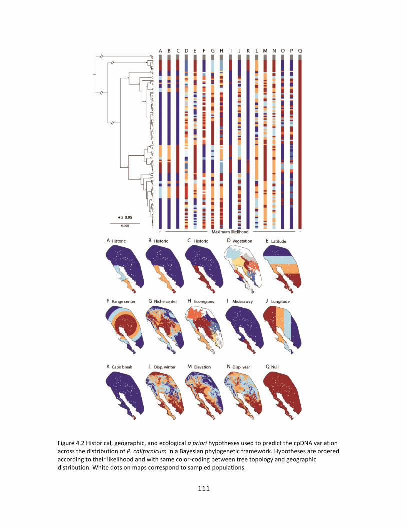
111

Figure 4.2 Historical, geographic, and ecological a priori hypotheses used to predict the cpDNA variation across the distribution of P. californicum in a Bayesian phylogenetic framework. Hypotheses are ordered according to their likelihood and with same color-coding between tree topology and geographic distribution. White dots on maps correspond to sampled populations.

112

The models with the second and third largest marginal likelihoods (B and C in Fig.

4.2) were also based on historical hypotheses nested within the best model, and

correspond to the northward marine transgression related to isolation of the Cape region

by the Isthmus of La Paz and formation of the Gulf of California. In order of likelihood,

remaining hypotheses were Shreve’s vegetation regionalization (C and D); distance to

geographic range center, distance to ecological niche centroid, and ecoregions (F-H);

elevation and disperser suitability (M-N); and lastly host species and the null hypothesis

(P-Q). Testing these hypotheses omitting the highly divergent population 225 did not

change these results (Table S4.2).

Present-Last Glacial Maximum suitability

All niche models performed significantly better than random expectations (P < 0.001;

Appendix S4). Thresholded suitability maps for mistletoe, hosts, and the disperser for the

present corresponded well to known ranges of each species (Fig. 4.3). Last Glacial

Maximum predictions showed some differences in amount of area predicted as suitable

for P. californicum and its hosts, depending on which global circulation model was used.

For P. californicum, projections showed relatively smaller ranges mostly restricted to

southwestern Arizona and parts of California in CCSM, in MIROC extending into Arizona,

central Baja California, and northwestern Sonora; P. nitens predictions were similar in

both scenarios, preserving most of its range in the present across the Sonoran Desert.

Both LGM models showed suitable areas for P. californicum in the Lower Colorado River

Valley, north of La Paz in the Cape, and in a coastal area in western Sonora. All host

species except P. glandulosa showed reductions in distributional areas; A. greggii and P.

113

velutina showed similar patterns, with their ranges split in two regions, one in the Lower

Colorado River Valley and the other in southern Sonora, whereas Cercidium species had

most of their suitable areas in southern coastal Sonora. Overall, these predictions showed

the largest accumulation of LGM host suitability in the Lower Colorado River Valley, along

the coast of Sonora, and in the eastern Cape region in the Baja California Peninsula (Figs.

4.3 and 4.4, Fig. S4.1).

Figure 4.3 Potential distribution for the mistletoe (Phoradendron californicum), its hosts (richness), and disperser (Phainopepla nitens) under current climate and two LGM climate scenarios (CCSM and MIROC).

114

Host and mistletoe macrofossils

The subfossil record from packrat middens of hosts and mistletoe has been found in caves

across the Sonoran and Chihuahuan deserts, indicating drastic changes in species

composition and highly dynamic distributional areas related to climate oscillations (see

Appendix S3). Most host fossils were from the Sonoran Desert, most abundant since 13

kya and for the mistletoe since 6.4 kya (see Appendix S3). Two of the most common host

species, A. greggii and P. velutina, were the oldest in the fossil record and were also

associated with two of the most frequent haplotypes (Fig. 4.4 and Fig. S4.1).

115

Figure 4.4 (A) Phoradendron californicum haplotype network for the three cpDNA concatenated regions colored by host species, excluding haplotypes from clade 4. (B) Potential distribution for mistletoe (inset) and hosts distributions during the LGM (21 kya) according to the MIROC climate scenario, showing geographic locations of most frequent haplotypes and macrofossil localities with mistletoe or hosts.

116

Discussion

The phylogeny of P. californicum inferred from cpDNA, was most probable under a model

reflecting a series of geologic events related to formation of the Baja California Peninsula

and seaways across it in the Pliocene and the Pleistocene. This view, however, is

complemented with that of a more dynamic distributional history associated to

continuous interaction with hosts in the Sonoran and Mojave deserts, as inferred from

niche model projections based on Pleistocene climate and fossil record.

Mistletoe phylogeny and phylogeographic patterns

Analyses of cpDNA showed that at least four well-supported clades existed among

sampled populations of P. californicum; 35 haplotypes were identified, with three main

clades coincident between the estimated haplotype network and ultrametric tree. Both

sympatry and allopatry in geographic distributions of haplotypes in P. californicum’s gene

tree suggest that diverse processes of diversification have occurred simultaneously in the

Baja California Peninsula and the Sonoran Desert region. These patterns are especially

intriguing in the context of the seaway breaks hypotheses and the mechanisms of seed

dispersal of P. californicum.

The first pattern corresponds to clades 1 and 2, which are sympatric across the

northern Sonoran Desert, northern Baja California Peninsula, and southern Mojave Desert

(Fig. 4.1). This distribution suggests long distance dispersal of seeds, as presence of

haplotypes across the Gulf of California and their origin from non-sister clades cannot

support an old vicariant event without subsequent gene flow. The fleshy fruits of P.

californicum are dependent on birds for dispersal and germination (Larson 1996, Murphy

117

et al. 1993), thus we expect long-distance dispersal, or accumulation of numerous short-

distance dispersal events over extended geographic regions, causing little or no signal of

phylogeographic structure in the cpDNA (e.g., Duminil et al. 2007, Worth et al. 2010). The

pattern exhibited between northern clades (1 and 2) would support this hypothesis, given

its large distribution and lack of geographic exclusivity of haplotypes across the Gulf of

California.

The second pattern is depicted by clades 2 and 3, in which clade 3 occurs

exclusively in southern Baja California Peninsula, and by the separation of clade 4 in the

Cape region from the rest of P. californicum (Fig. 4.1). In this case, the phylogeographic

break between clades 2 and 3 is congruent with the midpeninsular seaway near the

Vizcaíno Desert c. 1 mya. The split between clade 4 and the rest of P. californicum is

coincident with the formation of the Isthmus of La Paz in the southern portion of the

peninsula 3-4 mya, which supports vicariant divergence (Murphy and Aguirre-León 2002,

Riddle et al. 2000; Fig. 4.1). Nevertheless, this clade corresponds to a single population in

the eastern Cape region, which has been recognized as a botanical region distinct from

the rest of the Baja California Peninsula (Shreve 1951), and is also distant from optimal

niche conditions, which would correspond to both lower abundance and genetic diversity

(Lira-Noriega and Manthey 2014, Martínez-Meyer et al. 2013) or niche divergence. The

presence of phylogeographic breaks in the southern Baja California lineages (clades 3 and

4) suggests that limited dispersal has been sustained under conditions that promote

isolation and limited post-divergence spread. However, if no changes are assumed in the

dispersal capabilities among lineages, presence of deep phylogenetic breaks in the Baja

118

California Peninsula cannot be solely explained by vicariance, suggesting that additional

biological and ecological attributes could have promoted restrictions in the dispersal of

seeds.

Our estimates of node ages for the MRCA are compatible with some of the

peninsular geological events for the general mutation rate (1.3-4.1 mya), but also with

some of the most recent climatic oscillations for the accelerated mutation rate (0.2-0.8

mya), which suggests that vicariance cannot be an exclusive explanation for the

phylogeographic patterns (Garrick et al. 2009, Grismer 2002). Given the parasitic nature

of P. californicum, an accelerated mutation rate in chloroplast regions would be more

adequate to calibrating node ages compared to other non-parasitic plants in the area

(Bromham et al. 2013). This effect would be reflected in differences of at least three to six

times of neutral nucleotide variability present from the three sampled non-coding

chloroplast regions, compared to previous estimates from endemic plants of the Baja

California Peninsula (πpsbA-trnH = 0.0013; Fehlberg and Ranker 2009; Table S4.3). Therefore,

it is likely that the dates estimated under accelerated rates coincide with vicariant

divergence between clade 4 and the rest of P. californicum, and divergence between

clades 2 and 3 would be mostly associated with ecological and environmental

mechanisms of divergence.

Historical and ecological hypotheses

Given the preponderance of environmental and ecological factors in seed dispersal (Cain

et al. 2000, Nathan 2006), these factors should be contrasted with the most parsimonious

vicariant hypotheses on the phylogeographic structure in P. californicum. When we tested

119

the cpDNA topology against historical, ecological, and geographic hypotheses, patterns of

lineage divergence were best explained when individuals were grouped in the four land

areas that correspond to the three major seaway breaks associated with the formation of

the Gulf of California and subsequent splits of the Baja California Peninsula (Riddle et al.

2000, Riddle and Hafner 2006). Assumptions of the multi-population coalescent model

used to estimate marginal likelihoods of these competing hypotheses are likely violated

by P. californicum, most notably the assumption of no post-divergence gene flow among

subpopulations. However, we expect violations of this assumption would weaken support

for the hypothesis based on historical vicariance. Thus, our findings support this model as

the best predictor of the genealogical history of the cpDNA, suggesting that these major

land areas were important in structuring populations of P. californicum at deeper

evolutionary timescales, and coincides with findings from previous phylogeographic

studies (Munguia-Vega 2011, Murphy and Aguirre-León 2002).

However, while these historic hypotheses are based on the assumption that

Pliocene/Pleistocene marine transgression events were responsible for the genetic

discontinuities (Lindell et al. 2006, Riddle et al. 2000), several evolutionary forces might

be equally capable of explaining this pattern (Garrick et al. 2009, Grismer 2002). For

example, periods of expansion and contraction of the species’ range related to climate

oscillations and changes in vegetation could result in similar genetic discontinuities

(Comes and Kadereit 1998, Grismer 2002). Accordingly, our results do not necessarily rule

out competing hypotheses, particularly at recent timescales. Rather, these processes may

be more significant at finer spatial and temporal scales compared to large-scale processes

120

in structuring lineages (e.g., Lira-Noriega et al. 2013). This could explain, for example, why

the hypothesis based on vegetation types follows the historical hypotheses in marginal

likelihood, which are then followed by the hypotheses based on other ecological and

geographic factors (Table 4.3, Fig. 2).

An alternative explanation to the larger-scale geologic events in genetically

structuring P. californicum and in favor of ecological processes is supported by haplotype

geographic distributions in the context of its hosts (Fig. 4.4 and Fig. S4.1). Although host

species and genera explain the overall evolutionary history of the cpDNA poorly (these

hypotheses had the smallest marginal likelihoods before the null hypothesis; Table 4.3),

haplotype networks suggest the possibility of continuous evolutionary pathways in

relation to host species. Among the 10 host species identified for the individuals used in

our analysis, Acacia greggii, Prosopis velutina, and P. glandulosa were the most frequent

hosts and perhaps drivers of haplotype differentiation, followed by the two Cercidium

species; coincidentally, these host species and the mistletoe have been recorded in

packrat middens around the Lower Colorado River Valley, allowing us to confirm their

distributions and associations (Fig. 4.4 and Fig. S4.1, Appendix S4.3).

Haplotype groupings according to host species reinforce the evidence of host

specialization previously reported in P. californicum. Using isozymes, Glazner et al. (1988)

concluded genetic differences and different rates of seed establishment existed

depending on whether P. californicum individuals were parasitic on A. greggii or Prosopis

glandulosa in populations from the Mojave and Colorado deserts. Later, in a cross-

establishment experiment in northern Baja California, Overton (1997) concluded that two

121

host-specific types existed in P. californicum, one that primarily infects Acacia and

Cercidium, and another infecting Prosopis, but he did not find differences in

establishment of seeds from Acacia or Prosopis on Olneya. These findings help to explain

why haplotypes associated with clade 1 and 3-A are represented by a combination of host

species corresponding mostly to Acacia and Cercidium, and haplotypes associating clade 2

to Prosopis, which allows us to speculate on relative roles of host distributions for the

phylogeography of P. californicum (see Fig. 4.4 and Fig. S4.1).

Present and past distributions

Ecological niche model transfers to LGM (21 kya) conditions and macrofossils from

packrat middens (13-4 kya) both indicate that P. californicum’s distribution was

fragmented by the colder climates during the last ice age (Fig.4; Appendix S4.3). Only one

host species (P. glandulosa) showed a potentially wider distribution across the North

American deserts during the LGM, and also in a packrat midden from the Chihuahuan

Desert, whereas the other four species showed large range reductions, retreating to

refugia in the lower Colorado River Valley in the northern Sonoran Desert, southwestern

Sonora, and parts of Baja California (Fig. 4.4 and Fig. S4.1).

Since the widest inferred climatic refugium of P. californicum in the LGM coincides

with distributions of two common hosts (A. greggii and P. velutina), the most frequent

haplotypes from the northern clades (clades 1 and 2; Figs. 1 and 4), and the disperser

could range over the mistletoe distribution during LGM (see Fig. 4.3), it is possible that

dispersal and gene flow could have persisted in this part of the distribution during harsher

climatic conditions, supporting the cpDNA phylogeographic patterns. Additionally,

122

macrofossils indicate compositional changes of plant communities in the region in

synchrony with paleoclimatic conditions, and the appearance of hosts and mistletoe at

around 13-4 kya indicates their more recent arrival, as well as contractions and

expansions of their ranges (McAuliffe and McDonald 2006, McAuliffe and Van Devender

1998, Van Devender 1990a, b).

Because ecological and biological features of seed dispersal cannot be assimilated

into cpDNA phylogeographic patterns without considering environmental changes, as

they can be strongly correlated to climatic shifts (Aguinagalde et al. 2005), the combined

lines of evidence from the phylogenetic analysis, the hypothesis testing, and past

distributions allow for better interpretation of the distribution and history in P.

californicum. In this paper, we covered as much of the phylogeographic pattern as was

feasible by sampling many populations and genes across the range of P. californicum,

rather than large numbers of individuals per population. This dataset should be adequate

to test a series of hypotheses and detect and understand potential distributional breaks.

We presented a novel use of multi-population coalescent models to test among a priori

hypotheses based on potential historical and ecological processes of population

differentiation. This approach allowed us to compare the probability of the sequence data

under each hypothesis while integrating out uncertainty in the gene tree, population

history, and demographic parameters. Similar approaches have been used for delimiting

species (Grummer et al. 2013). Although we were limited to a single locus, by integrating

over the genealogical and population history, the results should accurately reflect the

posterior uncertainty conditional on our data. This approach is easily extended to multi-

123

locus data and provides a useful tool for testing among competing models of

phylogeographical history in an objective statistical framework.

Acknowledgments

The authors thank Ben Wilder for obtaining samples from Tiburón and Angel de la Guarda

islands, Richard Felger and Pedro Peña for help with regionalization of the Sonoran

Desert, Joseph D. Manthey for advice on molecular analyses, and Farzana Ahmed for help

with DNA extractions. Comments from A. Townsend Peterson, Richard Glor and Emily

McTavish helped us to improve previous version of the manuscript. We thank curators

from ASU for permission to sample loaned specimens and from KANU for supporting this

project. A Young Researchers Award from the Global Biodiversity Information Facility

(GBIF), a Tinker Award from the University of Kansas Center of Latin American Studies,

and a University of Kansas Biodiversity Institute Panorama small grant award (Bunker

Fund) supported collecting trips. A.L.-N. received scholarship support from Consejo

Nacional de Ciencia y Tecnología, Mexico (189216).

124

References

Acevedo P, Jiménez-Valverde A, Lobo JM, Real R (2012) Delimiting the geographical background in species distribution modelling. Journal of Biogeography 39, 1383-1390.

Aguinagalde I, Hampe A, Mohanty A, Martin JP, Duminil J, Petit RJ (2005) Effects of life-history traits and species distribution on genetic structure at maternally inherited markers in European trees and shrubs. Journal of Biogeography 32, 329-339.

Alexander MP, Burns KJ (2006) Intraspecific phylogeography and adaptive divergence in the White-headed Woodpecker. Condor 108, 489-508.

Allouche O, Steinitz O, Rotem D, Rosenfeld A, Kadmon R (2008) Incorporating distance constraints into species distribution models. Journal of Applied Ecology 45, 599-609.

Amico GC, Nickrent DL (2009) Population structure and phylogeography of the mistletoes Tristerix corymbosus and T. aphyllus (Loranthaceae) using chloroplast DNA sequence variation. American Journal of Botany 96, 1571-1580.

Amico GC, Rodriguez-Cabal MA, Aizen MA (2011) Geographic variation in fruit colour is associated with contrasting seed disperser assemblages in a south-Andean mistletoe. Ecography 34, 318-326.

Anderson, R (1981) Population ecology of infectious disease agents. Pages 318-355 in May R, editor. Theoretical ecology. Principles and applications. Blackwell Scientific Publications, Oxford.

Anderson RP, Peterson AT, Gómez-Laverde M (2003) Using niche-based GIS modeling to test geographic predictions of competitive exclusion and competitive release in South American pocket mice. Oikos 98, 3-16.

Araujo MB, Luoto M (2007) The importance of biotic interactions for modelling species distributions under climate change. Global Ecology and Biogeography 16, 743-753.

Ashworth VETM (2000) Phylogenetic relationships in phoradendreae (Viscaceae) inferred from three regions of the nuclear ribosomal cistron. I. Major lineages and paraphyly of phoradendron. Systematic Botany 25, 349-370.

Aukema JE (2003) Vectors, viscin, and Viscaceae: Mistletoes as parasites, mutualists, and resources. Frontiers in Ecology 1, 212-219.

Aukema JE, Martínez del Rio C (2002a) Where does a fruit-eating bird deposit mistletoe seeds? Seed deposition patterns and an experiment. Ecology 83, 3489-3496.

125

Aukema JE, Martínez del Rio C. (2002b) Variation in mistletoe seed deposition: Effects of intra- and interspecific host characteristics. Ecography 25, 139-144.

Aukema JE (2001) Dispersal and spatial distribution of the desert mistletoe, Phoradendron californicum, at multiple scales: Patterns, processes and mechanisms. Ph.D. Thesis University of Arizona, Tucson, AZ.

Aukema JE (2004) Distribution and dispersal of desert mistletoes is scale-dependent, hierarchically nested. Ecography 27, 137-144.

Baatz M, Benz U, Dehghani S, Heynen M, Höltje A, Hofmann P, Lingenfelder I, Mimler M, Sohlbach M, Weber M, Willhauck G (2003) eCognition 3 user guide. Definiens Imaging, Munich, Germany.

Baele G, Lemey P, Bedford T, Rambaut A, Suchard MA, Alekseyenko AV (2012) Improving the accuracy of demographic and molecular clock model comparison while accommodating phylogenetic uncertainty. Molecular Biology and Evolution 29, 2157-2167.

Barrera-Guzmán AO, Mila B, Sánchez-González LA, Navarro-Sigüenza AG (2012) Speciation in an avian complex endemic to the mountains of Middle America (Ergaticus, Ayes: Parulidae). Molecular Phylogenetics and Evolution 62, 907-920.

Barve N, Barve V, Jiménez-Valverde A, Lira-Noriega A, Maher SP, Peterson AT, Soberón J, Villalobos F (2011) The crucial role of the accessible area in ecological niche modeling and species distribution modeling. Ecological Modelling 222, 1810-1819.

Begon M, Townsend CR, Harper JL (2006) Ecology: From individuals to ecosystems, 4th edn. Blackwell Publishing, Oxford, UK.

Borenstein M, Hedges LV, Higgins JPT, Rothstein HR (2009) Introduction to meta-analysis. John Wiley and Sons, Chichester, UK.

Bozinovic F, Calosi P, Spicer JI. 2011. Physiological correlates of geographic range in animals. Annual Review of Ecology, Evolution and Systematics 42, 155-179.

Bridle JR, Vines TH (2007) Limits to evolution at range margins: When and why does adaptation fail? Trends in Ecology and Evolution 22, 140-147.

Bromham L, Cowman P, Lanfear R (2013) Parasitic plants have increased rates of molecular evolution across all three genomes. BMC Evolutionary Biology 13, 126.

Brotons L, De Caceres M, Fall A, Fortin MJ (2012) Modeling bird species distribution change in fire prone Mediterranean landscapes: Incorporating species dispersal and landscape dynamics. Ecography 35, 458-467.

Brown JH (1984) On the relationship between abundance and distribution of species. American Naturalist 124, 255-279.

126

Brown JH, Stevens GC, Kaufman DM (1996) The geographic range: Size, shape, boundaries, and internal structure. Annual Review of Ecology and Systematics 27, 597-623.

Brussard PF (1984) Geographic patterns and environmental gradients-the central–marginal model in Drosophila revisited. Annual Review of Ecology and Systematics 15, 25-64.

Buckley LB, Urban MC, Angilletta MJ, Crozier LG, Rissler LJ, Sears MW (2010) Can mechanism inform species' distribution models? Ecology Letters 13, 1041-1054.

Cabral JS, Schurr FM (2010) Estimating demographic models for the range dynamics of plant species. Global Ecology and Biogeography 19, 85-97.

Cain ML, Milligan BG, Strand AE (2000) Long-distance seed dispersal in plant populations. American Journal of Botany 87, 1217-1227.

Callaway RM, Reinhart KO, Moore GW, Moore DJ, Pennings SC (2002) Epiphyte host preferences and host traits: Mechanisms for species-specific interactions. Oecologia 132, 221-230.

Carlo TA, Morales JM (2008) Inequalities in fruit-removal and seed dispersal: Consequences of bird behaviour, neighbourhood density and landscape aggregation. Journal of Ecology 96, 609-618.

Carnaval AC, Hickerson MJ, Haddad CFB, Rodrigues MT, Moritz C (2009) Stability predicts genetic diversity in the Brazilian Atlantic forest hotspot. Science 323, 785-789.

Chapman AD (2005) Principles and methods of data cleaning–primary species and species-occurrence data, version 1.0. Global Biodiversity Information Facility, Copenhagen.

Chapman JR, Nakagawa S, Coltman DW, Slate J, Sheldon BC (2009) A quantitative review of heterozygosity-fitness correlations in animal populations. Molecular Ecology 18, 2746-2765.

Chu M, Walsberg GE (1999) Phainopepla (Phainopepla nitens). The birds of North America, No. 415 (ed. by A. Poole & F. Gill). Birds of North America Inc., Philadelphia, PA.

Clark-Tapia R, Molina-Freaner F (2003) The genetic structure of a columnar cactus with a disjunct distribution: Stenocereus gummosus in the Sonoran desert. Heredity 90, 443-450.

Clay K, Dement D, Rejmanek M (1985) Experimental evidence for host races in mistletoe (Phoradendron tomentosum). American Journal of Botany 72, 1225-1231.

Collins WD, Bitz CM, Blackmon ML, Bonan GB, Bretherton CS, Carton JA, Chang P, Doney SC, Hack JJ, Henderson TB, Kiehl JT, Large WG, McKenna DS, Santer BD, Smith RD

127

(2006) The Community Climate System Model version 3 (CCSM3). Journal of Climate 19, 2122-2143.

Comes HP, Kadereit JW (1998) The effect of quaternary climatic changes on plant distribution and evolution. Trends in Plant Science 3, 432-438.

Cook RD (1977) Detection of influential observation in linear–regression. Technometrics 19, 15-18.

Cortes-Rodriguez N, Hernandez-Baños BE, Navarro-Siguenza AG, Peterson AT, Garcia-Moreno J (2008) Phylogeography and population genetics of the Amethyst-throated Hummingbird (Lampornis amethystinus). Molecular Phylogenetics and Evolution 48, 1-11.

Cowles RB (1936) The relation of birds to seed dispersal of the desert mistletoe. Madroño 3, 352-356.

Cunningham HR, Rissler LJ, Apodaca JJ (2009) Competition at the range boundary in the slimy salamander: Using reciprocal transplants for studies on the role of biotic interactions in spatial distributions. Journal of Animal Ecology, 78, 52-62.

de Souza Muñoz M, de Giovanni R, de Siqueira M, Sutton T, Brewer P, Pereira R, Canhos D, Canhos V (2011) openModeller: A generic approach to species’ potential distribution modelling. GeoInformatica 15, 111-135.

Dimmit MA (2000) Biomes and communities of the Sonoran Desert region. in S. J. Phillips and P. Wentworth Comus, editors. A natural history of the Sonoran Desert. Arizona-Sonora Desert Museum Press and University of California Press, Berkeley and Los Angeles, California.

Diniz J, Nabout JC, Bini LM, Soares TN, Telles MPD, de Marco P, Collevatti RG (2009) Niche modelling and landscape genetics of Caryocar brasiliense ("Pequi" tree: Caryocaraceae) in Brazilian Cerrado: An integrative approach for evaluating central-peripheral population patterns. Tree Genetics & Genomes 5, 617-627.

Dissanayake STM, Onal H, Westervelt JD, Balbach HE (2012) Incorporating species relocation in reserve design models: An example from Ft. Benning GA. Ecological Modelling, 224, 65-75.

Doyle JJ, Doyle JD (1987) A rapid DNA isolation procedure for small quantities of freash leaf tissue. Phytochemical Bulletin 19, 11-15.

Drummond AJ, Suchard MA, Xie D, Rambaut A (2012) Bayesian Phylogenetics with BEAUti and the BEAST 1.7. Molecular Biology and Evolution 29, 1969-1973.

Duminil J, Fineschi S, Hampe A, Jordano P, Salvini D, Vendramin GG, Petit RJ (2007) Can population genetic structure be predicted from life-history traits? American Naturalist 169, 662-672.

Easterling D R, Karl TR, Lawrimore JH, Del Greco SA (1999) United States historical climatology network daily temperature, precipitation, and snow data for 1871-

128

1997. ORNL/CDIAC-118, NDP-070. Carbon Dioxide Information Analysis Center, Oak Ridge National Laboratory, U.S. Department of Energy, Oak Ridge, Tennessee.

Eckert CG, Samis KE, Lougheed SC (2008) Genetic variation across species' geographical ranges: The central-marginal hypothesis and beyond. Molecular Ecology 17, 1170-1188.

Edgar RC (2004) MUSCLE: Multiple sequence alignment with high accuracy and high throughput. Nucleic Acids Research 32, 1792-1797.

Ehrich D, Alsos IG, Brochmann C (2008) Where did the northern peatland species survive the dry glacials: Cloudberry (Rubus chamaemorus) as an example. Journal of Biogeography 35, 801-814.

Eidesen PB, Alsos IG, Popp M, Stensrud O, Suda J, Brochmann C (2007) Nuclear vs. plastid data: Complex Pleistocene history of a circumpolar key species. Molecular Ecology 16, 3902-3925.

Eidesen PB, Carlsen T, Molau U, Brochmann C (2007) Repeatedly out of Beringia: Cassiope tetragona embraces the arctic. Journal of Biogeography 34, 1559-1574.

Elith J, Graham CH, Anderson RP, Dudik M, Ferrier S, Guisan A, Hijmans RJ, Huettmann F, Leathwick JR, Lehmann A, Li J, Lohmann LG, Loiselle BA, Manion G, Moritz C, Nakamura M, Nakazawa Y, Overton JM, Peterson AT, Phillips SJ, Richardson K, Scachetti-Pereira R, Schapire RE, Soberon J, Williams S, Wisz MS, Zimmermann NE (2006) Novel methods improve prediction of species' distributions from occurrence data. Ecography 29, 129-151.

ESRI. 2011. ArcGIS Desktop: Release 10. Redlands, California. Environmental Systems Research Institute.

Esselstyn JA, Evans BJ, Sedlock JL, Khan FAA, Heaney LR (2012) Single-locus species delimitation: A test of the mixed Yule-coalescent model, with an empirical application to Philippine round-leaf bats. Proceedings of the Royal Society B-Biological Sciences 279, 3678-3686.

Ezard T, Fujisawa T, Barraclough TC (2013) splits: Species' Limits by Threshold Statistics. R package version 1.0-18/45. http://R-Forge.R-project.org/projects/splits/.

Fehlberg SD, Ranker TA (2009) Evolutionary history and phylogeography of Encelia farinosa (Asteraceae) from the Sonoran, Mojave, and Peninsular Deserts. Molecular Phylogenetics and Evolution 50, 326-335.

Fischer G, Nachtergaele F, Prieler S, van Velthuizen HT, Verelst L, Wiberg D (2008) Global agro-ecological zones assessment for agriculture. International Institute for Applied Systems Analysis, Laxenburg, Austria and FAO, Rome, Italy.

Fortin MJ, Keitt TH, Maurer BA, Taper ML, Kaufman DM, Blackburn TM (2005) Species' geographic ranges and distributional limits: Pattern analysis and statistical issues. Oikos 108, 7-17.

129

Fujisawa T, Barraclough TG (2013) Delimiting species using Single-Locus Data and the Generalized Mixed Yule Coalescent Approach: A revised method and evaluation on simulated data sets. Systematic Biology 62, 707-724.

Galbreath KE, Cook JA (2004) Genetic consequences of Pleistocene glaciations for the tundra vole (Microtus oeconomus) in Beringia. Molecular Ecology 13, 135-148.

Galbreath KE, Cook JA, Eddingsaas AA, DeChaine EG. 2011. Diversity and demography in Beringia: Multilocus tests of paleodistribution models reveal the complex history of Arctic ground squirrels. Evolution 65, 1879-1896.

Gao QB, Zhang DJ, Duan YZ, Zhang FQ, Li YH, Fu PC, Chen SL (2012) Intraspecific divergences of Rhodiola alsia (Crassulaceae) based on plastid DNA and internal transcribed spacer fragments. Botanical Journal of the Linnean Society 168, 204-215.

Garcia D, Rodriguez-Cabal MA, Amico GC (2009) Seed dispersal by a frugivorous marsupial shapes the spatial scale of a mistletoe population. Journal of Ecology 97, 217-229.

Garcillán PP, Ezcurra E (2003) Biogeographic regions and β-diversity of woody dryland legumes in the Baja California peninsula. Journal of Vegetation Science 14, 859-868.

Garner TWJ, Pearman PB, Angelone S (2004) Genetic diversity across a vertebrate species' range: A test of the central-peripheral hypothesis. Molecular Ecology 13, 1047-1053.

Garrick RC, Nason JD, Meadows CA, Dyer RJ (2009) Not just vicariance: Phylogeography of a Sonoran Desert euphorb indicates a major role of range expansion along the Baja peninsula. Molecular Ecology 18, 1916-1931.

Gaston KJ (2003) The structure and dynamics of geographic ranges. Oxford University Press, Oxford, UK.

Gaston KJ, Genney DR, Thurlow M, Hartley SE (2004) The geographical range structure of the holly leaf-miner. IV. Effects of variation in host-plant quality. Journal of Animal Ecology 73, 911-924.

Genini J, Côrtes MC, Guimarães PR, Galetti M (2012) Mistletoes play different roles in a modular host–parasite network. Biotropica 44, 171-178.

Glazner JT, Devlin B, Ellstrand NC (1988) Biochemical and morphological evidence for host race evolution in Desert Mistletoe, Phoradendron californicum (Viscaceae). Plant Systematics and Evolution 161, 13-21.

Grismer L (2002) A re-evaluation of the evidence for a mid-Pleistocene mid-peninsular seaway in Baja California: A reply to Riddle et al. Herpetological Review 33, 15-16.

130

Grummer JA, Bryson RW, Reeder TW (2013) Species delimitation using Bayes factors: Simulations and application to the Sceloporus scalaris species group (Squamata: Phrynosomatidae). Systematic Biology syt069.

Grus WE, Graves GR, Glenn TC (2009) Geographic variation in the mitochondrial control region of Black-throated Blue Warblers (Dendroica caerulescens). Auk 126, 198-210.

Guisan A, Zimmermann NE (2000) Predictive habitat distribution models in ecology. Ecological Modelling 135, 147-186.

Hafner DJ, Riddle BR (2011) Boundaries and barriers of North American warm deserts: An evolutionary perspective. In Upchurch P, McGowan A, Slater C (eds) Palaeogeography and palaeobiogeography: Biodiversity in space and time. CRC Press.

Hagen A (2003) Fuzzy set approach to assessing similarity of categorical maps. International Journal of Geographical Information Science 17, 235-249.

Haigh SL (1996) Saltcedar (Tamarix ramosissima), an uncommon host for desert mistletoe (Phoradendron californicum). Great Basin Naturalist 56, 186-187.

Haldane JBS (1956) The Relation between density regulation and natural selection. Proceedings of the Royal Society Series B-Biological Sciences 145, 306-308.

Hastings A, Petrovskii S, Morozov A (2011) Spatial ecology across scales. Biology Letters 7, 163-165.

Hasumi H, Emori S (2004) K-1 coupled gcm (miroc) description. Center for Climate System Research, University of Tokyo, Tokyo.

Heibl C, Calenge C (2013) phyloclim: Integrating phylogenetics and climatic niche modeling. R package version 0.9-3. Available at: http://cran.r-project.org/web/packages/phyloclim.

Heikkinen RK, Luoto M, Virkkala R, Pearson RG, Korber JH (2007) Biotic interactions improve prediction of boreal bird distributions at macro-scales. Global Ecology and Biogeography 16, 754-763.

Hengeveld R, Haeck J (1982) The distribution of abundance. I. Measurements. Journal of Biogeography 9, 303-316.

Hijmans RJ, Cameron SE, Parra JL, Jones PG, Jarvis A (2005) Very high resolution interpolated climate surfaces for global land areas. International Journal of Climatology 25, 1965-1978.

Holt RD (2003) On the evolutionary ecology of species' ranges. Evolutionary Ecology Research 5, 159-178.

131

Holt RD, Gomulkiewicz R (1997) The evolution of species’ niches: A population dynamic perspective. In Othmer H, Adler F, Lewis M, Dallon J (eds) Case studies in mathematical modelling: Ecology, physiology, and cell biology, pp. 25-50. Prentice–Hall, Englewood Cliffs, New Jersey.

Holt RD, Keitt TH (2005) Species' borders: A unifying theme in ecology. Oikos 108, 3-6.

Homer CCH, Yang L, Wylie B, Coan M (2004) Development of a 2001 National Landcover Database for the United States. Photogrammetric Engineering and Remote Sensing 70, 829-840.

Hutchinson GE (1957) Population Studies - Animal Ecology and Demography - Concluding Remarks. Cold Spring Harbor Symposia on Quantitative Biology 22, 415-427.

Hutchinson GE (1978) An introduction to population ecology. Yale University Press, New Haven, USA.

Jackson ST, Overpeck JT (2000) Responses of plant populations and communities to environmental changes of the late Quaternary. Paleobiology 26, 194-220.

James FC, Johnston RF, Wamer NO, Niemi GJ, Boecklen WJ (1984) The Grinnellian niche of the Wood Thrush. American Naturalist 124, 17-30.

Jerome CA, Ford BA (2002) The discovery of three genetic races of the dwarf mistletoe Arceuthobium americanum (Viscaceae) provides insight into the evolution of parasitic angiosperms. Molecular Ecology 11, 387-405.

Joly S, Stevens MI, van Vuuren BJ (2007) Haplotype networks can be misleading in the presence of missing data. Systematic Biology 56, 857-862.

Kass RE, Raftery AE (1995) Bayes factors. Journal of the American Statistical Association 90, 773-795.

Kavanagh PH, Burns KC (2012) Mistletoe macroecology: Spatial patterns in species diversity and host use across Australia. Biological Journal of the Linnean Society 106, 459-468.

Kawecki TJ (2008) Adaptation to marginal habitats. Annual Review of Ecology and Systematics 39, 321-342.

Kearney M, Porter W (2009) Mechanistic niche modelling: Combining physiological and spatial data to predict species' ranges. Ecology Letters 12, 334-350.

Kearney M, Wintle BA, Porter W (2010) Correlative and mechanistic models of species distribution provide congruent forecasts under climate change. Conservation Letters 3, 203-213.

132

Keller SR, Olson MS, Silim S, Schroeder W, Tiffin P (2010) Genomic diversity, population structure, and migration following rapid range expansion in the Balsam Poplar, Populus balsamifera. Molecular Ecology 19, 1212-1226.

Kimura M, Clegg SM, Lovette IJ, Holder KR, Girman DJ, Mila B, Wade P, Smith TB (2002) Phylogeographical approaches to assessing demographic connectivity between breeding and overwintering regions in a Nearctic-Neotropical warbler (Wilsonia pusilla). Molecular Ecology 11, 1605-1616.

Kuijt, J. (2003) Monograph of Phoradendron (Viscaceae). Systematic Botany Monographs 66, 1-643.

Lack JB, Pfau RS, Wilson GM (2010) Demographic history and incomplete lineage sorting obscure population genetic structure of the Texas mouse (Peromyscus attwateri). Journal of Mammalogy 91, 314-325.

Laliberte AS, Rango A, Havstad KM, Paris JF, Beck RF, McNeely R, Gonzalez AL (2004) Object-oriented image analysis for mapping shrub encroachment from 1937 to 2003 in southern New Mexico. Remote Sensing of Environment 93, 198-210.

Larson DL (1996) Seed dispersal by specialist versus generalist foragers: The plant's perspective. Oikos 76, 113-120.

Lavorel S, Stafford Smith MS, Reid N (1999) Spread of mistletoes (Amyema preissii) in fragmented Australian woodlands: A simulation study. Landscape ecology 14, 147-160.

Lei SA (1999) Age, size and water status of Acacia gregii influencing the infection and reproductive success of Phoradendron californicum. American Midland Naturalist 141, 358-365.

Leimu R, Mutikainen P, Koricheva J, Fischer M (2006) How general are positive relationships between plant population size, fitness, and genetic variation? Journal of Ecology 94, 942-952.

Lemieux CJ, Beechey TJ, Scott DJ, Gray PA (2011) The state of climate change adaptation in Canada's protected areas sector. Canadian Geographer 55, 301-317.

Levin SA (1992) The problem of pattern and scale in ecology. Ecology 73, 1943-1967.

Levin SA, Pacala SW (1997) Theories of simplification and scaling of spatially distributed species. Pages 271-295 in Tilman D, Kareiva P, editors. Spatial ecology: The role of space in population dynamics and intersepecific interactions. Princeton University Press, Princeton, New Jersey, USA.

Li XC, Yin H, Li K, Gao XY (2012) Population genetic structure and historical demography of the ground beetle Pheropsophus jessoensis from the Tsinling–Dabashan

133

Mountains, central China based on mitochondrial DNA analysis. Zoological Science 29, 238-246.

Liaw A, Wiener M (2002) Classification and regression by randomForest. R News 2, 18--22.

Lindell J, Ngo A, Murphy RW (2006) Deep genealogies and the mid-peninsular seaway of Baja California. Journal of Biogeography 33, 1327-1331.

Lira-Noriega A, Manthey JD (2014) Relationship of genetic diversity and niche centrality: A survey and analysis. Evolution doi:10.1111/evo.12343.

Lira-Noriega A, Peterson AT (In press) Range-wide ecological niche comparisons of parasite, hosts and dispersers in a vector-borne plant parasite system. Journal of Biogeography.

Lira-Noriega A, Soberon J, Miller CP (2013) Process-based and correlative modeling of desert mistletoe distribution: A multiscalar approach. Ecosphere 4, art99.

Liu CR, Berry PM, Dawson TP, Pearson RG (2005) Selecting thresholds of occurrence in the prediction of species distributions. Ecography 28, 385-393.

Liu RS, Martínez del Rio C, Wu JH (2011) Spatiotemporal variation of mistletoes: A dynamic modeling approach. Bulletin of Mathematical Biology 73, 1794-1811.

Loveless MD, Hamrick JL (1984) Ecological determinants of genetic-structure in plant-populations. Annual Review of Ecology and Systematics 15, 65-95.

Lozier JD, Strange JP, Stewart IJ, Cameron SA (2011) Patterns of range–wide genetic variation in six North American bumble bee (Apidae: Bombus) species. Molecular Ecology 20, 4870-4888.

MacArthur RH (1972) Geographical ecology: Patterns in the distribution of species. Harper and Row, New York, USA.

Mackey BG, Lindenmayer DB (2001) Towards a hierarchical framework for modelling the spatial distribution of animals. Journal of Biogeography 28, 1147-1166.

Maher SP, Ellis C, Gage KL, Enscore RE, Peterson AT (2010) Range-wide determinants of plague distribution in North America. American Journal of Tropical Medicine and Hygiene 83, 736-742.

Manthey JD, Klicka J, Spellman GM (2011) Cryptic diversity in a widespread North American songbird: Phylogeography of the Brown Creeper (Certhia americana). Molecular Phylogenetics and Evolution 58, 502-512.

Marquardt ES, Pennings SC (2010) Constraints on host use by a parasitic plant. Oecologia, 164, 177-184.

134

Martínez del Rio C, Silva A, Medel R, Hourdequin M (1996) Seed dispersers as disease vectors: Bird transmission of mistletoe seeds to plant hosts. Ecology 77, 912-921.

Martínez-Meyer E, Díaz-Porras D, Peterson AT, Yáñez-Arenas C (2013) Ecological niche structure and rangewide abundance patterns of species. Biology Letters 9, 20120637.

Mathiasen RL, Nickrent DL, Shaw DC, Watson DM (2008) Mistletoes: Pathology, systematics, ecology and management. Plant Disease 92, 988-1006.

McAuliffe JR, McDonald EV (2006) Holocene environmental change and vegetation contraction in the Sonoran Desert. Quaternary Research 65, 204-215.

McAuliffe JR, Van Devender TR (1998) A 22,000-year record of vegetation change in the north-central Sonoran Desert. Palaeogeography Palaeoclimatology Palaeoecology 141, 253-275.

McDonald DE, Daniels SR (2012) Phylogeography of the Cape velvet worm (Onychophora: Peripatopsis capensis) reveals the impact of Pliocene/Pleistocene climatic oscillations on Afromontane forest in the Western Cape, South Africa. Journal of E Evolutionary Biology 25, 824-835.

Moeller DA, Geber MA, Tiffin P (2011) Population genetics and the evolution of geographic range limits in an annual plant. American Naturalist 178, S44-S61.

Monahan WB (2009) A mechanistic niche model for measuring species' distributional responses to seasonal temperature gradients. PloS ONE 4:e7921.

Montaño-Centellas FA (2013) Effectiveness of mistletoe seed dispersal by tyrant flycatchers in a mixed Andean landscape. Biotropica 45, 209-216.

Morand S, Krasnov BR (eds) (2010) The biogeography of host–parasite interactions. Oxford University Press, New York.

Morin X, Thuiller W (2009) Comparing niche- and process-based models to reduce prediction uncertainty in species range shifts under climate change. Ecology 90, 1301-1313.

Mort ME, Soltis DE, Soltis PS, Francisco-Ortega J, Santos-Guerra A (2001) Phylogenetic relationships and evolution of Crassulaceae inferred from matK sequence data. American Journal of Botany 88, 76-91.

Munguia-Vega A (2011) Habitat fragmentation in small vertebrates from the Sonoran Desert in Baja California. The University of Arizona.

Murphy RW, Aguirre-León G (2002) The nonavian reptiles: Origins and evolution. In Case TJ, Cody ML, Ezcurra E (eds) A new island biogeography of the Sea of Cortéz, pp. 181-220. Oxford University Press, New York.

135

Murphy SR, Reid N, Yan ZG, Venables WN (1993) Differential passage time of mistletoe fruits through the gut of honeyeaters and flowerpeckers: Effects on seedling establishment. Oecologia 93, 171-176.

Nason JD, Hamrick JL, Fleming TH (2002) Historical vicariance and postglacial colonization effects on the evolution of genetic structure in Lophocereus, a Sonoran Desert columnar cactus. Evolution 56, 2214-2226.

Nathan R (2006) Long-distance dispersal of plants. Science 313, 786-788.

Nickrent DL (2002) Mistletoe phylogenetics: Current relationships gained from analysis of DNA sequences. Proceedings of the forty-eighth western international forest disease work conference, 48-57.

Nickrent DL, Stell AL (1990) Electrophoretic evidence for genetic differentiation in two host races of hemlock dwarf mistletoe (Arceuthobium tsugense). Biochemical Systematics and Ecology 18, 267-280.

Norton DA, Smith MS (1999) Why might roadside mulgas be better mistletoe hosts? Australian Journal of Ecology 24, 193-198.

Norton DA, Ladley JJ, Owen HJ (1997) Distribution and population structure of the loranthaceous mistletoes Alepis flavida, Peraxilla colensoi, and Peraxilla tetrapetala within two New Zealand Nothofagus forests. New Zealand Journal of Botany, 35, 323-336.

Nylander JAA, Wilgenbusch JC, Warren DL, Swofford DL (2008) AWTY (are we there yet?): A system for graphical exploration of MCMC convergence in Bayesian phylogenetics. Bioinformatics 24, 581-583.

Olson DM, Dinerstein E, Wikramanayake ED, Burgess ND, Powell GVN, Underwood EC, D’amico JA, Itoua I, Strand HE, Morrison JC, Loucks CJ, Allnutt TF, Ricketts TH, Kura Y, Lamoreux JF, Wettengel, WW, Hedao P, Kassem KR (2001) Terrestrial ecoregions of the world: A new map of life on Earth. BioScience 51, 933-938.

Oomen RA, Reudink MW, Nocera JJ, Somers CM, Green MC, Kyle CJ (2011) Mitochondrial evidence for panmixia despite perceived barriers to gene flow in a widely distributed waterbird. Journal of Heredity 102, 584-+.

Ortego J, Riordan EC, Gugger PF, Sork VL (2012) Influence of environmental heterogeneity on genetic diversity and structure in an endemic southern Californian oak. Molecular Ecology 21, 3210-3223.

Overton JM (1997) Host specialization and partial reproductive isolation in desert mistletoe (Phoradendron californicum). Southwestern Naturalist 42, 201-209.

Overton JM (1994) Dispersal and infection in mistletoe metapopulations. Journal of Ecology 82, 711-723.

136

Overton JM (1996) Spatial autocorrelation and dispersal in mistletoes: Field and simulation results. Vegetatio 125, 83-98.

Paul JR, Sheth SN, Angert AL (2011) Quantifying the impact of gene flow on phenotype-environment mismatch: A demonstration with the scarlet monkeyflower Mimulus cardinalis. American Naturalist 178, S62-S79.

Pearson RG, Dawson TP (2003) Predicting the impacts of climate change on the distribution of species: Are bioclimate envelope models useful? Global Ecology and Biogeography 12, 361-371.

Pearson RG, Raxworthy CJ, Nakamura M, Peterson AT (2007) Predicting species distributions from small numbers of occurrence records: A test case using cryptic geckos in Madagascar. Journal of Biogeography 34, 102-117.

Pérez-Alquicira J, Molina-Freaner FE, Piñero D, Weller SG, Martínez-Meyer E, Rozas J, Domínguez CA (2010) The role of historical factors and natural selection in the evolution of breeding systems of Oxalis alpina in the Sonoran desert 'Sky Islands'. Journal of Evolutionary Biologye 23, 2163-2175.

Peterson AT, Soberon J, Pearson RG, Anderson RP,Martinez-Meyer E, Nakamura M, and Araujo MB. (2011) Ecological niches and geographic distributions Princeton University Press, Princeton, New Jersey, USA.

Peterson AT, Papeş M, Soberon J (2008) Rethinking receiver operating characteristic analysis applications in ecological niche modeling. Ecological Modelling 213, 63-72.

Peterson AT, Papeş M, Eaton M. (2007) Transferability and model evaluation in ecological niche modeling: A comparison of GARP and Maxent. Ecography 30, 550-560.

Pfeifer M, Schatz B, Pico FX, Passalacqua NG, Fay MF, Carey PD, Jeltsch F (2009) Phylogeography and genetic structure of the orchid Himantoglossum hircinum (L.) Spreng. across its European central-marginal gradient. Journal of Biogeography 36, 2353-2365.

Phillips SJ, Anderson RP, Schapire RE (2006) Maximum entropy modeling of species geographic distributions. Ecological Modelling 190, 231-259.

Pons J, Barraclough TG, Gomez-Zurita J, Cardoso A, Duran DP, Hazell S, Kamoun S, Sumlin WD, Vogler AP (2006) Sequence-based species delimitation for the DNA taxonomy of undescribed insects. Systematic Biology 55, 595-609.

Primack R (2006) Essentials of conservation biology. Sinauer, Sunderland, Massachusetts.

Pulliam HR (1988) Sources, sinks, and population regulation. American Naturalist 132, 652-661.

137

Pulliam HR (2000) On the relationship between niche and distribution. Ecology Letters. 3:349-361.

R Development Core Team (2013) R: A language and environment for statistical computing. R Foundation for Statistical Computing, Vienna, Austria: R Foundation for Statistical Computing.

R Development Core Team (2011) R: A language and environment for statistical computing. R Foundation for Statistical Computing, Vienna, Austria: R Foundation for Statistical Computing.

R Development Core Team (2012) A language and environment for statistical computing. R Foundation for Statistical Computing, Vienna, Austria: R Foundation for Statistical Computing.

Rambaut A, Drummond A (2007) Tracer v 1.5. Available from http://beast.bio.ed.ac.uk/Tracer.

Ramos ACS, Lemos-Filho JP, Ribeiro RA, Santos FR, Lovato MB (2007) Phylogeography of the tree Hymenaea stigonocarpa (Fabaceae : Caesalpinioideae) and the influence of quaternary climate changes in the Brazilian cerrado. Annals of Botany 100, 1219-1228.

Rangel TF, Diniz-Filho JAF, Bini LM (2010) SAM: A comprehensive application for spatial analysis in macroecology. Ecography 33, 6-50.

Rapoport EH (1982) Areography: Geographical strategies of species. Pergamon Press, Oxford.

Rawsthorne J, Watson DM, Roshier DA (2012) The restricted seed rain of a mistletoe specialist. Journal of Avian Biology 43, 9-14.

Real R, Barbosa AM, Rodriguez A, Garcia FJ, Vargas JM, Palomo LJ, Delibes M (2009) Conservation biogeography of ecologically interacting species: The case of the Iberian lynx and the European rabbit. Diversity and Distributions 15, 390-400.

Rebernig CA, Schneeweiss GM, Bardy KE, Schonswetter P, Villaseñor JL, Obermayer R, Stuessy TF, Weiss-Schneeweiss, H (2010) Multiple Pleistocene refugia and Holocene range expansion of an abundant southwestern American desert plant species (Melampodium leucanthum, Asteraceae). Molecular Ecology 19, 3421-3443.

Reding DM, Bronikowski AM, Johnson WE, Clark WR (2012) Pleistocene and ecological effects on continental-scale genetic differentiation in the bobcat (Lynx rufus). Molecular Ecology 21, 3078-3093.

Reed DH, Frankham R (2003) Correlation between fitness and genetic diversity. Conservation Biology 17, 230-237.

138

Reid NM, Carstens BC (2012) Phylogenetic estimation error can decrease the accuracy of species delimitation: A Bayesian implementation of the general mixed Yule-coalescent model. BMC Evolutionary Biology 12, 196.

Reid N (1991) Coevolution of mistletoes and frugivorous birds. Australian Journal of Ecology 16, 457-469.

Ribeiro RA, Lemos JP, Ramos ACS, Lovato MB (2011) Phylogeography of the endangered rosewood Dalbergia nigra (Fabaceae): Insights into the evolutionary history and conservation of the Brazilian Atlantic Forest. Heredity 106, 46-57.

Riddle B, Hafner D, Alexander L, Jaeger J (2000) Cryptic vicariance in the historical assembly of a Baja California peninsular desert biota. Proceedings of the National Academy of Sciences of the United States of America 97, 14438-14443.

Riddle BR, Hafner DJ (2006) A step-wise approach to integrating phylogeographic and phylogenetic biogeographic perspectives on the history of a core North American warm deserts biota. Journal of Arid Environments 66, 435-461.

Rist L, Uma Shaanker R, Ghazoul J (2011) The spatial distribution of mistletoe in a southern Indian tropical forest at multiple scales. Biotropica 43, 50-57.

Roberts DR, Hamann A (2012) Predicting potential climate change impacts with bioclimate envelope models: A palaeoecological perspective. Global Ecology and Biogeography 21, 121-133.

Robertson MP, Peter CI, Villet MH, Ripley BS (2003) Comparing models for predicting species' potential distributions: A case study using correlative and mechanistic predictive modelling techniques. Ecological Modelling 164, 153-167.

Sagarin RD, Gaines SD (2002) The 'abundant centre' distribution: To what extent is it a biogeographical rule? Ecology Letters 5, 137-147.

Sauer JR, Hines JE, Fallon J, Pardieck KL, Ziolkowski Jr DJ, Link WA (2011) The North American Breeding Bird Survey, Results and Analysis 1966-2010. Version 12.07.2011. USGS Patuxent Wildlife Research Center, Laurel, Maryland.

Schaal BA, Hayworth DA, Olsen KM, Rauscher JT, Smith WA (1998) Phylogeographic studies in plants: Problems and prospects. Molecular Ecology 7, 465-474.

Schurr FM, Pagel J, Cabral JS, Groeneveld J, Bykova O, O'Hara RB, Hartig F, Kissling WD, Linder HP, Midgley GF, Schroder B, Singer A, Zimmermann NE (2012) How to understand species' niches and range dynamics: A demographic research agenda for biogeography. Journal of Biogeography 39, 2146-2162.

Segovia RA, Pérez MF, Hinojosa LF (2012) Genetic evidence for glacial refugia of the temperate tree Eucryphia cordifolia (Cunoniaceae) in southern South America. American Journal of Botany 99, 121-129.

139

Sexton JP, McIntyre PJ, Angert AL, Rice KJ (2009) Evolution and ecology of species range limits. Annual Review of Ecology Evolution and Systematics 40, 415-436.

Sgariglia EA, Burns KJ (2003) Phylogeography of the California Thrasher (Toxostoma redivivum) based on nested-clade analysis of mitochondrial-DNA variation. Auk 120, 346-361.

Shaw J, Lickey EB, Schilling EE, Small RL (2007) Comparison of whole chloroplast genome sequences to choose noncoding regions for phylogenetic studies in angiosperms: The tortoise and the hare III. American Journal of Botany 94, 275-288.

Shreve F (1951) Vegetation of the Sonoran Desert. Publ. Carnegie Inst. Washington No. 591. Reprinted as vol. 1, Shreve F, Wiggins IL Vegetation and flora of the Sonoran Desert. Stanford University Press, Stanford, CA.

Smith BT, Escalante P, Banos BEH, Navarro-Sigüenza AG, Rohwer S, Klicka J (2011) The role of historical and contemporary processes on phylogeographic structure and genetic diversity in the Northern Cardinal, Cardinalis cardinalis. BMC Evolutionary Biology 11.

Soberón J (2007) Grinnellian and Eltonian niches and geographic distributions of species. Ecology Letters 10, 1115-1123.

Soberón JM (2010) Niche and area of distribution modeling: A population ecology perspective. Ecography 33, 159-167.

Soberón J, Nakamura M (2009) Niches and distributional areas: Concepts, methods, and assumptions. Proceedings of the National Academy of Sciences of the United States of America 106, 19644-19650.

Soberón J, Peterson AT (2005) Interpretation of models of fundamental ecological niches and species' distributional areas. Biodiversity Informatics 2, 1-10.

Spellman GM, Klicka J (2006) Testing hypotheses of Pleistocene population history using coalescent simulations: Phylogeography of the pygmy nuthatch (Sitta pygmaea). Proceedings of the Royal Society B-Biological Sciences 273, 3057-3063.

Spellman GM, Klicka J (2007) Phylogeography of the white-breasted nuthatch (Sitta carolinensis): Diversification in North American pine and oak woodlands. Molecular Ecology 16 1729-1740.

Spellman GM, Riddle B, Klicka J (2007) Phylogeography of the mountain chickadee (Poecile gambeli): Diversification, introgression, and expansion in response to Quaternary climate change. Molecular Ecology 16 1055-1068.

Stanton S, Honnay O, Jacquemyn H, Roldan-Ruiz I (2009) A comparison of the population genetic structure of parasitic Viscum album from two landscapes differing in degree of fragmentation. Plant Systematics and Evolution 281, 161-169.

Swofford DL (2003) PAUP* Phylogenetic analysis using parsimony (*and other methods). Version 4. Sinauer Associates.

140

Templeton AR, Crandall KA, Sing CF (1992) A Cladistic-Analysis of Phenotypic Associations with Haplotypes Inferred from Restriction Endonuclease Mapping and DNA-Sequence Data .3. Cladogram Estimation. Genetics 132, 619-633.

Temunovic M, Franjic J, Satovic Z, Grgurev M, Frascaria-Lacoste N, Fernandez-Manjarre JF (2012) Environmental heterogeneity explains the genetic structure of continental and Mediterranean populations of Fraxinus angustifolia Vahl. Plos One, 7

Thuiller W, Albert CH, Dubuis A, Randin C, Guisan A (2010) Variation in habitat suitability does not always relate to variation in species' plant functional traits. Biology Letters 6, 120-123.

Torres NM, De Marco P, Santos T, Silveira L, Jacomo ATD, Diniz JAF (2012) Can species distribution modelling provide estimates of population densities? A case study with jaguars in the Neotropics. Diversity and Distributions 18, 615-627.

Udvardy MDF (1969) Dynamic zoogeography. Van Nostrand Reinhold Company, New York.

Van Devender TR (1990a) Late Quaternary vegetation and climate of the Chihuahuan Desert, United States and Mexico. In Betancourt JL, Van Devender TR, Martin PS (eds) Pacrat middens: The last 40,000 years of biotic change, pp. 104-133. The University of Arizona Press, Tucson, AZ.

Van Devender TR (1990b) Late Quaternary vegetation and climate of the Sonoran Desert, United States and Mexico. In Betancourt JL, Van Devender TR, Martin PS (eds) Pacrat middens: The last 40,000 years of biotic change, pp. 134-165. The University of Arizona Press, Tucson, AZ.

Vandermeer JH, Goldberg DE (2003) Population ecology: First principles. Princeton University Press, New Jersey, USA.

VanDerWal J, Shoo LP, Johnson CN, Williams SE (2009) Abundance and the environmental niche: Environmental suitability estimated from niche models predicts the upper limit of local abundance. American Naturalist 174, 282-291.

Visser H, de Nijs T (2006) The Map Comparison Kit. Environmental Modelling & Software 21, 346-358.

Vucetich JA, Waite TA (2003) Spatial patterns of demography and genetic processes across the species' range: Null hypotheses for landscape conservation genetics. Conservation Genetics 4, 639-645.

Wagner V, Durka W, Hensen I (2011) Increased genetic differentiation but no reduced genetic diversity in peripheral vs. central populations of a steppe grass. American Journal of Botany 98, 1173-1179.

Walsberg GE (1975) Digestive adaptations of Phainopepla nitens associated with the eating of mistletoe berries. Condor 77, 169-174.

141

Warren DL, Glor RE, Turelli M (2010) ENMTools: A toolbox for comparative studies of environmental niche models. Ecography 33, 607-611.

Warren DL, Glor RE, Turelli M (2008) Environmental niche equivalency versus conservatism: Quantitative approaches to niche evolution. Evolution 62, 2868-2883.

Waterhouse AM, Procter JB, Martin DMA, Clamp M, Barton GJ (2009) Jalview Version 2-a multiple sequence alignment editor and analysis workbench. Bioinformatics 25, 1189-1191.

Watson DM (2001) Mistletoe - a kesystone resource in forests and woodlands worldwide. Annual Review of Ecology and Systematics 32, 219-249.

Watson DM (2009) Determinants of parasitic plant distribution: The role of host quality. Botany-Botanique 87, 16-21.

Weksler M, Lanier HC, Olson LE (2010) Eastern Beringian biogeography: Historical and spatial genetic structure of singing voles in Alaska. Journal of Biogeography 37, 1414-1431.

Westergaard KB, Alsos IG, Popp M, Engelskjon T, Flatberg KI, Brochmann C (2011) Glacial survival may matter after all: Nunatak signatures in the rare European populations of two west-arctic species. Molecular Ecology 20, 376-393.

Whittaker PL (1984) The insect fauna of mistletoe (Phoradendron tomentosum, Loranthaceae) in southern Texas. The Southwestern Naturalist 29, 435-444.

Whittaker RJ, Willis KJ, Field R (2001) Scale and species richness: Towards a general, hierarchical theory of species diversity. Journal of Biogeography 28, 453-470.

Wiens JA (1989) Spatial scaling in ecology. Functional Ecology 3, 385-397.

Wiens JA (2000) Ecological heterogeneity: An ontogeny of concepts and approaches. Pages 9-31 in Hutchings MJ, John EA, Stewart AJA editors. The ecological consequences of environmental heterogeneity: The 40th symposium of the British Ecological Society, held at the University of Sussex, 23-25 March 1999. Blackwell Science, Sussex, UK.

Wilson KA, Westphal MI, Possingham HP, Elith J (2005) Sensitivity of conservation planning to different approaches to using predicted species distribution data. Biological Conservation 122, 99-112.

Wisz MS, Pottier J, Kissling WD, Pellissier L, Lenoir J, Damgaard CF, Dormann CF, Forchhammer MC, Grytnes JA, Guisan A, Heikkinen RK, Hoye TT, Kuhn I, Luoto M, Maiorano L, Nilsson MC, Normand S, Ockinger E, Schmidt NM, Termansen M, Timmermann A, Wardle DA, Aastrup P, Svenning JC (2013) The role of biotic interactions in shaping distributions and realised assemblages of species: Implications for species distribution modelling. Biological Reviews 88, 15-30.

142

Wolfe KH, Li WH, Sharp PM (1987) Rates of nucleotide substitution vary greatly among plant mitochondrial, chloroplast, and nuclear DNA. Proceedings of the National Academy of Sciences United States of America 84, 9054-9058.

Wood SN (2011) Fast stable restricted maximum likelihood and marginal likelihood estimation of semiparametric generalized linear models. Journal of the Royal Statistical Society Series B-Statistical Methodology 73, 3-36.

Worth JRP, Jordan GJ, Marthick JR, Mckinnon GE, Vaillancourt RE (2010) Chloroplast evidence for geographic stasis of the Australian bird-dispersed shrub Tasmannia lanceolata (Winteraceae). Molecular Ecology 19, 2949-2963.

Xie W, Lewis PO, Fan Y, Kuo L, Chen MH (2011) Improving marginal likelihood estimation for Bayesian phylogenetic model selection. Systematic Biology 60,150-160.

Yang F-S, Li Y-F, Ding XIN, Wang X-Q (2008) Extensive population expansion of Pedicularis longiflora (Orobanchaceae) on the Qinghai-Tibetan Plateau and its correlation with the Quaternary climate change. Molecular Ecology 17, 5135-5145.

Zuber D, Widmer A (2009) Phylogeography and host race differentiation in the European mistletoe (Viscum album L.). Molecular Ecology 18, 1946-1962.

143

Appendices

Appendix 1.1 Derivation of the formulas for the process-based model.

We modeled population dynamics of mistletoes using formalism borrowed from

metapopulation theory. We consider a grid of cells of maximum resolution,

corresponding to the typical area under an average-sized legume tree, on the order of 20

m2. We now construct coarser-resolution grids that contain maximum-resolution cells,

asking for the proportion of the coarse-resolution cells that is occupied by infected trees

(number of high-resolution infected cells/total number of cells in the coarse-resolution

unit), that is, by trees with at least one individual of mistletoe. Let i = 1, 2, 3…n denote the

coarse-resolution cells in the grid. Then the following equation is proposed (Hanski 1999):

1ii i i i

dpc p e p

dt ,

where pi is the probability of species presence in cell i, dpi/dt is its time derivative; ci is

the colonization rate in cell i and ei is the extinction rate in cell i. In words, the growth rate

of the proportion of space occupied by the mistletoe in the i-th cell increases

proportionally to a colonization rate ci and in inverse proportion to an extinction rate ei.

Now, imagine that the grid is coarsened, such that inside a new larger cell J (we use a

capital letter to denote an aggregate of smaller cells) is a collection of the higher-

resolution cells i. This can be achieved by using square cells and doubling the side of the

144

cells in the grid: one doubling contains 4 smaller cells, another doubling contains 16

smaller cells, and so on.

We are interested in the mean value of the occupied proportion of a cell:

1

| |J i

i J

p pJ

,

and therefore:

1 1 1

1| | | | | |

Ji i i i i i i i i i

i J i J i J i J i J i J

dp dp c p e p c c p e p

dt dt J J J

.

Now, we make the reasonable assumption that, inside every larger cell J, the values of

colonization rate and extinction rates can be approximated as their averages over the

smaller cells:

1

| |

Ji i i i i J J J J J

i J i J i J

dpc c p e p c c p e p

dt J

,

which, in the steady state, implies:

* JJ

J J

cp

c e

.

The equations for the colonization and extinction rates are postulated after consideration

of the BAM diagram: colonization is proportional to the abundance of birds and trees in

cell J, and inversely related to the distance to other occupied cells (Hanski 1999):

, 0

2

1 1

exp1

nJ K

J K

K K

dc L

b

,

145

where β0 and β1 represent parameters to be fitted, dJ,K is a measure of distance

(Euclidean, corrected by topography) between cells J and K; bK is the density of birds

present in cell K, and LK is the number of trees in cell K. These three last quantities are

obtained from data (see Methods for more detail).

The extinction rate in cell J is assumed to be a function of the distance from the centroid

of the fundamental niche of the species to the environmental data in the cell, as

represented in an ellipsoid:

1T

J J Je f

x μ Σ x μ ,

where the parameters and represent fitted values that define a multi-normal

distribution of optimal, ideal environmental preferences. The values of xJ represent the

observed environmental values in the cell J.

146

Table S1.1. Summary of model performance. For each model it is shown the area

predicted as suitable or unsuitable after using a minimum training presence threshold

and the partial AUC ratio statistics.

Resolution Model Area 0 Area 1 AUC min AUC max AUC mean AUC s.d.

1 km

process 178579 1181774 0.973 1.156 1.030 0.026

g_dh 1076124 290319 1.122 1.550 1.321 0.069

g_c 704875 662533 1.045 1.299 1.132 0.051

g_cdh 1051953 314490 1.142 1.601 1.418 0.082

gm_dh 694012 672431 1.035 1.270 1.089 0.026

gm_c 561353 806055 1.029 1.328 1.073 0.027

gm_cdh 825443 541000 1.041 1.265 1.089 0.026

m_dh 538460 827983 1.110 1.530 1.297 0.087

m_c 226380 1141028 1.048 1.270 1.110 0.042

m_cdh 492828 873615 1.092 1.556 1.242 0.063

5 km

process 15471 38806 1.096 1.247 1.180 0.019

g_dh 42135 12142 1.049 1.428 1.111 0.034

g_c 25470 28807 1.032 1.281 1.091 0.035

g_cdh 41897 12380 1.040 1.348 1.107 0.035

gm_dh 26332 27651 1.036 1.570 1.239 0.089

gm_c 22009 32268 1.038 1.276 1.130 0.049

gm_cdh 36712 17271 1.184 1.599 1.397 0.088

m_dh 18661 35322 1.114 1.617 1.276 0.081

m_c 11120 43157 1.068 1.332 1.129 0.031

m_cdh 33715 20268 1.099 1.510 1.360 0.084

10 km

process 2817 10764 1.106 1.272 1.203 0.024

g_dh 10880 2701 1.043 1.309 1.099 0.030

g_c 10567 3014 1.025 1.240 1.073 0.026

g_cdh 10008 3573 1.071 1.552 1.165 0.062

gm_dh 6099 7482 1.125 1.604 1.344 0.095

gm_c 5731 7850 1.044 1.296 1.125 0.051

gm_cdh 8471 5110 1.073 1.635 1.259 0.129

m_dh 4583 8998 1.050 1.575 1.288 0.083

m_c 3331 10250 1.094 1.267 1.149 0.036

m_cdh 6775 6806 1.068 1.532 1.245 0.054

20 km

process 542 2866 1.082 1.278 1.188 0.030

g_dh 2724 684 1.053 1.357 1.124 0.040

g_c 1591 1817 1.028 1.279 1.087 0.035

g_cdh 2670 738 1.052 1.614 1.122 0.042

gm_dh 1472 1935 1.089 1.558 1.280 0.105

gm_c 1070 2337 1.022 1.254 1.070 0.028

gm_cdh 2345 1062 1.030 1.454 1.089 0.037

m_dh 746 2617 1.112 1.546 1.270 0.065

m_c 951 2412 1.081 1.330 1.182 0.031

m_cdh 1340 2023 1.111 1.624 1.272 0.074

50 km

process 157 377 1.124 1.285 1.227 0.027

g_dh 436 91 1.018 1.074 1.038 0.008

g_c 189 345 1.019 1.214 1.075 0.033

g_cdh 408 119 1.039 1.256 1.094 0.028

gm_dh 137 397 1.002 1.420 1.056 0.053

gm_c 196 338 1.033 1.241 1.133 0.055

gm_cdh 352 182 1.077 1.563 1.249 0.098

m_dh 143 384 1.105 1.571 1.289 0.101

m_c 136 398 1.103 1.257 1.178 0.024

m_cdh 212 322 1.167 1.595 1.337 0.085

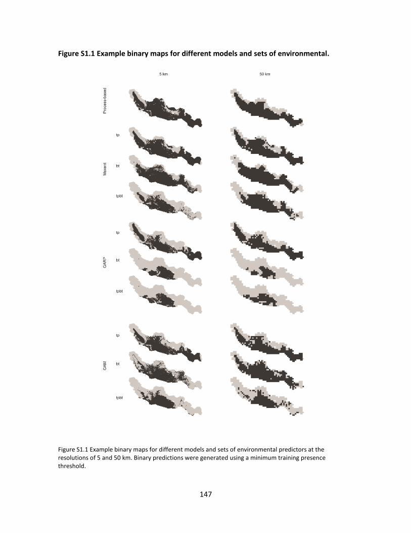
147

Figure S1.1 Example binary maps for different models and sets of environmental.

Figure S1.1 Example binary maps for different models and sets of environmental predictors at the resolutions of 5 and 50 km. Binary predictions were generated using a minimum training presence threshold.

148

Figure S1.2 Example of map comparison with fuzzy Kappa statistic.

Figure S1.2 Example of map comparison with fuzzy Kappa statistic. In (a), note an overall high coincidence between two maps (in this case GARP disperser + host versus GARP climate + disperser + host), and in (b), note an example of low coincidence (GARP climate + disperser + host versus Maxent climate) at a resolution of 5 km.

149

Appendix 2.1 Model evaluation.

Dispersers models Area 0 Area 1 Prob. presence Trials Successes P value

Bombycilla cedrorum year-round 852077 369828 0.302665101 100 85 P < 0.001 Bombycilla cedrorum winter 878446 343459 0.281084863 100 87 P < 0.001 Turdus migratorius year-round 654438 695037 0.515042517 100 96 P < 0.001 Turdus migratorius winter 1068742 280733 0.208031271 100 94 P < 0.001 Hosts overall 141687 159738 0.529942772 100 100 P < 0.001 Phoradendron californicum (mistletoe) 52979 24782 0.318694461 60 60 P < 0.001 Melanerpers uropygialis year-round 125740 20265 0.138796617 100 95 P < 0.001 Melanerpers uropygialis winter 115414 30591 0.209520222 100 64 P < 0.001 Mimus polyglottos year-round 537241 276777 0.340013366 99 95 P < 0.001 Mimus polyglottos winter 542948 271070 0.333002464 96 86 P < 0.001 Myadestes townsendi year-round 809985 187892 0.188291743 100 90 P < 0.001 Myadestes townsendi winter 847374 150503 0.150823198 100 78 P < 0.001 Phainopepla nitens year-round 206097 84569 0.290949062 100 94 P < 0.001 Phainopepla nitens winter 197028 93638 0.322149821 100 96 P < 0.001 Sialis currucoides year-round 849502 267653 0.23958448 100 88 P < 0.001 Sialis currucoides winter 989582 127573 0.114194539 100 82 P < 0.001 Sialia mexicana year-round 277017 132639 0.323781417 100 90 P < 0.001 Sialia mexicana winter 367000 42656 0.104126389 100 77 P < 0.001 Sialia sialis year-round 505821 301210 0.373232255 100 96 P < 0.001 Sialia sialis winter 566506 240525 0.298036878 100 99 P < 0.001 Toxostoma curvirostre year-round 151930 142866 0.484626657 100 98 P < 0.001 Toxostoma curvirostre winter 219811 74985 0.254362339 100 89 P < 0.001

Hosts models (*species with < 14 occurrence localities)

Acacia constricta mistletoe-infected* P < 0.001 Acacia constricta overall 100077 37909 0.27473077 100 89 P < 0.001 Acacia greggii mistletoe-infected 127697 11636 0.083512162 50 46 P < 0.001 Acacia greggii overall 51610 87723 0.629592415 100 91 P < 0.001 Cercidium floridum mistletoe-infected* P < 0.001 Cercidium floridum overall 47971 17015 0.261825624 99 78 P < 0.001 Cercidium microphyllum mistletoe-infected 33316 7166 0.177016946 10 6 P < 0.001 Cercidium microphyllum overall 22738 17744 0.438318265 100 91 P < 0.001 Larrea tridentata mistletoe-infected* P = 0.001 Larrea tridentata overall 117968 73107 0.382608923 100 95 P < 0.001 Olneya tesota mistletoe-infected 35380 12130 0.255314671 15 10 P < 0.001 Olneya tesota overall 34448 13062 0.274931593 100 90 P < 0.001 Prosopis glandulosa mistletoe-infected 268096 24224 0.08286809 14 13 P < 0.001 Prosopis glandulosa overall 169737 122583 0.419345238 99 79 P < 0.001 Prosopis velutina mistletoe-infected 114227 23994 0.173591567 20 19 P < 0.001 Prosopis velutina overall 121153 17068 0.123483407 100 65 P < 0.001

150

Appendix 3.1 Genetic diversity measures and estimates of distances to geographic

range center and niche centroid.

See Supporting Information—Appendix S1—online in Lira-Noriega A, Manthey JD (2014)

Relationship of genetic diversity and niche centrality: A survey and analysis. Evolution

doi:10.1111/evo.12343

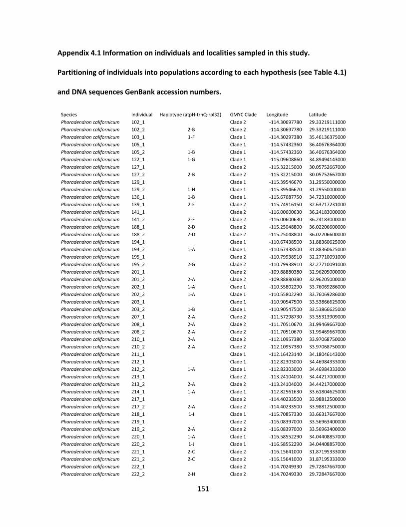
151

Appendix 4.1 Information on individuals and localities sampled in this study.

Partitioning of individuals into populations according to each hypothesis (see Table 4.1)

and DNA sequences GenBank accession numbers.

Species Individual Haplotype (atpH-trnQ-rpl32) GMYC Clade Longitude Latitude

Phoradendron californicum 102_1 Clade 2 -114.30697780 29.33219111000

Phoradendron californicum 102_2 2-B Clade 2 -114.30697780 29.33219111000

Phoradendron californicum 103_1 1-F Clade 1 -114.30297380 35.46136375000

Phoradendron californicum 105_1 Clade 1 -114.57432360 36.40676364000

Phoradendron californicum 105_2 1-B Clade 1 -114.57432360 36.40676364000

Phoradendron californicum 122_1 1-G Clade 1 -115.09608860 34.89494143000

Phoradendron californicum 127_1 Clade 2 -115.32215000 30.05752667000

Phoradendron californicum 127_2 2-B Clade 2 -115.32215000 30.05752667000

Phoradendron californicum 129_1 Clade 1 -115.39546670 31.29550000000

Phoradendron californicum 129_2 1-H Clade 1 -115.39546670 31.29550000000

Phoradendron californicum 136_1 1-B Clade 1 -115.67687750 34.72310000000

Phoradendron californicum 139_1 2-E Clade 2 -115.74916150 32.63717231000

Phoradendron californicum 141_1 Clade 2 -116.00600630 36.24183000000

Phoradendron californicum 141_2 2-F Clade 2 -116.00600630 36.24183000000

Phoradendron californicum 188_1 2-D Clade 2 -115.25048800 36.02206600000

Phoradendron californicum 188_2 2-D Clade 2 -115.25048800 36.02206600000

Phoradendron californicum 194_1 Clade 1 -110.67438500 31.88360625000

Phoradendron californicum 194_2 1-A Clade 1 -110.67438500 31.88360625000

Phoradendron californicum 195_1 Clade 2 -110.79938910 32.27710091000

Phoradendron californicum 195_2 2-G Clade 2 -110.79938910 32.27710091000

Phoradendron californicum 201_1 Clade 2 -109.88880380 32.96205000000

Phoradendron californicum 201_2 2-A Clade 2 -109.88880380 32.96205000000

Phoradendron californicum 202_1 1-A Clade 1 -110.55802290 33.76069286000

Phoradendron californicum 202_2 1-A Clade 1 -110.55802290 33.76069286000

Phoradendron californicum 203_1 Clade 1 -110.90547500 33.53866625000

Phoradendron californicum 203_2 1-B Clade 1 -110.90547500 33.53866625000

Phoradendron californicum 207_1 2-A Clade 2 -111.57298730 33.55313909000

Phoradendron californicum 208_1 2-A Clade 2 -111.70510670 31.99469667000

Phoradendron californicum 208_2 2-A Clade 2 -111.70510670 31.99469667000

Phoradendron californicum 210_1 2-A Clade 2 -112.10957380 33.97068750000

Phoradendron californicum 210_2 2-A Clade 2 -112.10957380 33.97068750000

Phoradendron californicum 211_1 Clade 1 -112.16423140 34.18046143000

Phoradendron californicum 212_1 Clade 1 -112.82303000 34.46984333000

Phoradendron californicum 212_2 1-A Clade 1 -112.82303000 34.46984333000

Phoradendron californicum 213_1 Clade 2 -113.24104000 34.44217000000

Phoradendron californicum 213_2 2-A Clade 2 -113.24104000 34.44217000000

Phoradendron californicum 214_1 1-A Clade 1 -112.82561630 33.61804625000

Phoradendron californicum 217_1 Clade 2 -114.40233500 33.98812500000

Phoradendron californicum 217_2 2-A Clade 2 -114.40233500 33.98812500000

Phoradendron californicum 218_1 1-I Clade 1 -115.70857330 33.66317667000

Phoradendron californicum 219_1 Clade 2 -116.08397000 33.56963400000

Phoradendron californicum 219_2 2-A Clade 2 -116.08397000 33.56963400000

Phoradendron californicum 220_1 1-A Clade 1 -116.58552290 34.04408857000

Phoradendron californicum 220_2 1-J Clade 1 -116.58552290 34.04408857000

Phoradendron californicum 221_1 2-C Clade 2 -116.15641000 31.87195333000

Phoradendron californicum 221_2 2-C Clade 2 -116.15641000 31.87195333000

Phoradendron californicum 222_1 Clade 2 -114.70249330 29.72847667000

Phoradendron californicum 222_2 2-H Clade 2 -114.70249330 29.72847667000

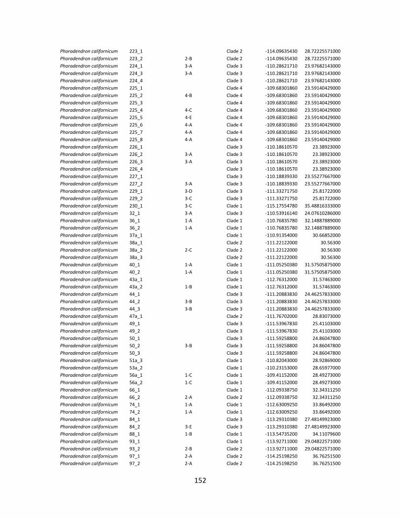
152

Phoradendron californicum 223_1 Clade 2 -114.09635430 28.72225571000

Phoradendron californicum 223_2 2-B Clade 2 -114.09635430 28.72225571000

Phoradendron californicum 224_1 3-A Clade 3 -110.28621710 23.97682143000

Phoradendron californicum 224_3 3-A Clade 3 -110.28621710 23.97682143000

Phoradendron californicum 224_4 Clade 3 -110.28621710 23.97682143000

Phoradendron californicum 225_1 Clade 4 -109.68301860 23.59140429000

Phoradendron californicum 225_2 4-B Clade 4 -109.68301860 23.59140429000

Phoradendron californicum 225_3 Clade 4 -109.68301860 23.59140429000

Phoradendron californicum 225_4 4-C Clade 4 -109.68301860 23.59140429000

Phoradendron californicum 225_5 4-E Clade 4 -109.68301860 23.59140429000

Phoradendron californicum 225_6 4-A Clade 4 -109.68301860 23.59140429000

Phoradendron californicum 225_7 4-A Clade 4 -109.68301860 23.59140429000

Phoradendron californicum 225_8 4-A Clade 4 -109.68301860 23.59140429000

Phoradendron californicum 226_1 Clade 3 -110.18610570 23.38923000

Phoradendron californicum 226_2 3-A Clade 3 -110.18610570 23.38923000

Phoradendron californicum 226_3 3-A Clade 3 -110.18610570 23.38923000

Phoradendron californicum 226_4 Clade 3 -110.18610570 23.38923000

Phoradendron californicum 227_1 Clade 3 -110.18839330 23.55277667000

Phoradendron californicum 227_2 3-A Clade 3 -110.18839330 23.55277667000

Phoradendron californicum 229_1 3-D Clade 3 -111.33271750 25.81722000

Phoradendron californicum 229_2 3-C Clade 3 -111.33271750 25.81722000

Phoradendron californicum 230_1 3-C Clade 1 -115.17554780 35.48816333000

Phoradendron californicum 32_1 3-A Clade 3 -110.53916140 24.07610286000

Phoradendron californicum 36_1 1-A Clade 1 -110.76835780 32.14887889000

Phoradendron californicum 36_2 1-A Clade 1 -110.76835780 32.14887889000

Phoradendron californicum 37a_1 Clade 1 -110.91354000 30.66852000

Phoradendron californicum 38a_1 Clade 2 -111.22122000 30.56300

Phoradendron californicum 38a_2 2-C Clade 2 -111.22122000 30.56300

Phoradendron californicum 38a_3 Clade 2 -111.22122000 30.56300

Phoradendron californicum 40_1 1-A Clade 1 -111.05250380 31.57505875000

Phoradendron californicum 40_2 1-A Clade 1 -111.05250380 31.57505875000

Phoradendron californicum 43a_1 Clade 1 -112.76312000 31.57463000

Phoradendron californicum 43a_2 1-B Clade 1 -112.76312000 31.57463000

Phoradendron californicum 44_1 Clade 3 -111.20883830 24.46257833000

Phoradendron californicum 44_2 3-B Clade 3 -111.20883830 24.46257833000

Phoradendron californicum 44_3 3-B Clade 3 -111.20883830 24.46257833000

Phoradendron californicum 47a_1 Clade 2 -111.76702000 28.83073000

Phoradendron californicum 49_1 Clade 3 -111.53967830 25.41103000

Phoradendron californicum 49_2 Clade 3 -111.53967830 25.41103000

Phoradendron californicum 50_1 Clade 3 -111.59258800 24.86047800

Phoradendron californicum 50_2 3-B Clade 3 -111.59258800 24.86047800

Phoradendron californicum 50_3 Clade 3 -111.59258800 24.86047800

Phoradendron californicum 51a_3 Clade 1 -110.82043000 28.92869000

Phoradendron californicum 53a_2 Clade 1 -110.23153000 28.65977000

Phoradendron californicum 56a_1 1-C Clade 1 -109.41152000 28.49273000

Phoradendron californicum 56a_2 1-C Clade 1 -109.41152000 28.49273000

Phoradendron californicum 66_1 Clade 1 -112.09338750 32.34311250

Phoradendron californicum 66_2 2-A Clade 2 -112.09338750 32.34311250

Phoradendron californicum 74_1 1-A Clade 1 -112.63009250 33.86492000

Phoradendron californicum 74_2 1-A Clade 1 -112.63009250 33.86492000

Phoradendron californicum 84_1 Clade 3 -113.29310380 27.48149923000

Phoradendron californicum 84_2 3-E Clade 3 -113.29310380 27.48149923000

Phoradendron californicum 88_1 1-B Clade 1 -113.54735200 34.11079600

Phoradendron californicum 93_1 Clade 1 -113.92711000 29.04822571000

Phoradendron californicum 93_2 2-B Clade 2 -113.92711000 29.04822571000

Phoradendron californicum 97_1 2-A Clade 2 -114.25198250 36.76251500

Phoradendron californicum 97_2 2-A Clade 2 -114.25198250 36.76251500

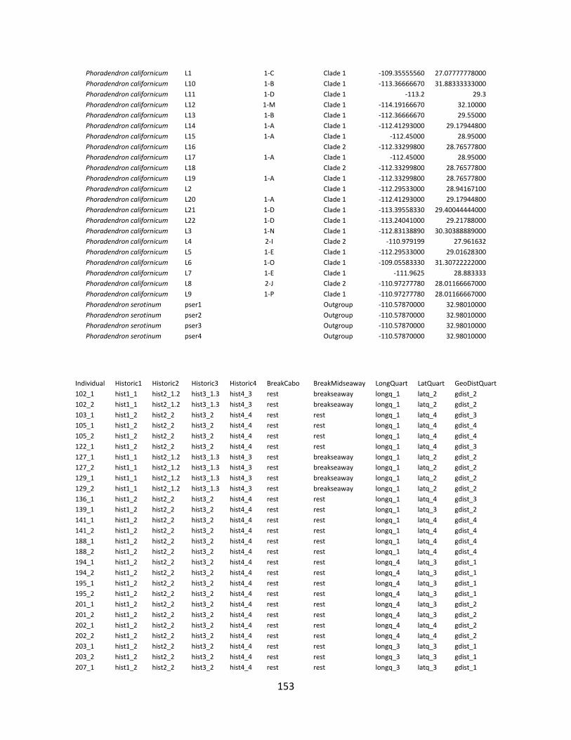
153

Phoradendron californicum L1 1-C Clade 1 -109.35555560 27.07777778000

Phoradendron californicum L10 1-B Clade 1 -113.36666670 31.88333333000

Phoradendron californicum L11 1-D Clade 1 -113.2 29.3

Phoradendron californicum L12 1-M Clade 1 -114.19166670 32.10000

Phoradendron californicum L13 1-B Clade 1 -112.36666670 29.55000

Phoradendron californicum L14 1-A Clade 1 -112.41293000 29.17944800

Phoradendron californicum L15 1-A Clade 1 -112.45000 28.95000

Phoradendron californicum L16 Clade 2 -112.33299800 28.76577800

Phoradendron californicum L17 1-A Clade 1 -112.45000 28.95000

Phoradendron californicum L18 Clade 2 -112.33299800 28.76577800

Phoradendron californicum L19 1-A Clade 1 -112.33299800 28.76577800

Phoradendron californicum L2 Clade 1 -112.29533000 28.94167100

Phoradendron californicum L20 1-A Clade 1 -112.41293000 29.17944800

Phoradendron californicum L21 1-D Clade 1 -113.39558330 29.40044444000

Phoradendron californicum L22 1-D Clade 1 -113.24041000 29.21788000

Phoradendron californicum L3 1-N Clade 1 -112.83138890 30.30388889000

Phoradendron californicum L4 2-I Clade 2 -110.979199 27.961632

Phoradendron californicum L5 1-E Clade 1 -112.29533000 29.01628300

Phoradendron californicum L6 1-O Clade 1 -109.05583330 31.30722222000

Phoradendron californicum L7 1-E Clade 1 -111.9625 28.883333

Phoradendron californicum L8 2-J Clade 2 -110.97277780 28.01166667000

Phoradendron californicum L9 1-P Clade 1 -110.97277780 28.01166667000

Phoradendron serotinum pser1 Outgroup -110.57870000 32.98010000

Phoradendron serotinum pser2 Outgroup -110.57870000 32.98010000

Phoradendron serotinum pser3 Outgroup -110.57870000 32.98010000

Phoradendron serotinum pser4 Outgroup -110.57870000 32.98010000

Individual Historic1 Historic2 Historic3 Historic4 BreakCabo BreakMidseaway LongQuart LatQuart GeoDistQuart

102_1 hist1_1 hist2_1.2 hist3_1.3 hist4_3 rest breakseaway longq_1 latq_2 gdist_2

102_2 hist1_1 hist2_1.2 hist3_1.3 hist4_3 rest breakseaway longq_1 latq_2 gdist_2

103_1 hist1_2 hist2_2 hist3_2 hist4_4 rest rest longq_1 latq_4 gdist_3

105_1 hist1_2 hist2_2 hist3_2 hist4_4 rest rest longq_1 latq_4 gdist_4

105_2 hist1_2 hist2_2 hist3_2 hist4_4 rest rest longq_1 latq_4 gdist_4

122_1 hist1_2 hist2_2 hist3_2 hist4_4 rest rest longq_1 latq_4 gdist_3

127_1 hist1_1 hist2_1.2 hist3_1.3 hist4_3 rest breakseaway longq_1 latq_2 gdist_2

127_2 hist1_1 hist2_1.2 hist3_1.3 hist4_3 rest breakseaway longq_1 latq_2 gdist_2

129_1 hist1_1 hist2_1.2 hist3_1.3 hist4_3 rest breakseaway longq_1 latq_2 gdist_2

129_2 hist1_1 hist2_1.2 hist3_1.3 hist4_3 rest breakseaway longq_1 latq_2 gdist_2

136_1 hist1_2 hist2_2 hist3_2 hist4_4 rest rest longq_1 latq_4 gdist_3

139_1 hist1_2 hist2_2 hist3_2 hist4_4 rest rest longq_1 latq_3 gdist_2

141_1 hist1_2 hist2_2 hist3_2 hist4_4 rest rest longq_1 latq_4 gdist_4

141_2 hist1_2 hist2_2 hist3_2 hist4_4 rest rest longq_1 latq_4 gdist_4

188_1 hist1_2 hist2_2 hist3_2 hist4_4 rest rest longq_1 latq_4 gdist_4

188_2 hist1_2 hist2_2 hist3_2 hist4_4 rest rest longq_1 latq_4 gdist_4

194_1 hist1_2 hist2_2 hist3_2 hist4_4 rest rest longq_4 latq_3 gdist_1

194_2 hist1_2 hist2_2 hist3_2 hist4_4 rest rest longq_4 latq_3 gdist_1

195_1 hist1_2 hist2_2 hist3_2 hist4_4 rest rest longq_4 latq_3 gdist_1

195_2 hist1_2 hist2_2 hist3_2 hist4_4 rest rest longq_4 latq_3 gdist_1

201_1 hist1_2 hist2_2 hist3_2 hist4_4 rest rest longq_4 latq_3 gdist_2

201_2 hist1_2 hist2_2 hist3_2 hist4_4 rest rest longq_4 latq_3 gdist_2

202_1 hist1_2 hist2_2 hist3_2 hist4_4 rest rest longq_4 latq_4 gdist_2

202_2 hist1_2 hist2_2 hist3_2 hist4_4 rest rest longq_4 latq_4 gdist_2

203_1 hist1_2 hist2_2 hist3_2 hist4_4 rest rest longq_3 latq_3 gdist_1

203_2 hist1_2 hist2_2 hist3_2 hist4_4 rest rest longq_3 latq_3 gdist_1

207_1 hist1_2 hist2_2 hist3_2 hist4_4 rest rest longq_3 latq_3 gdist_1

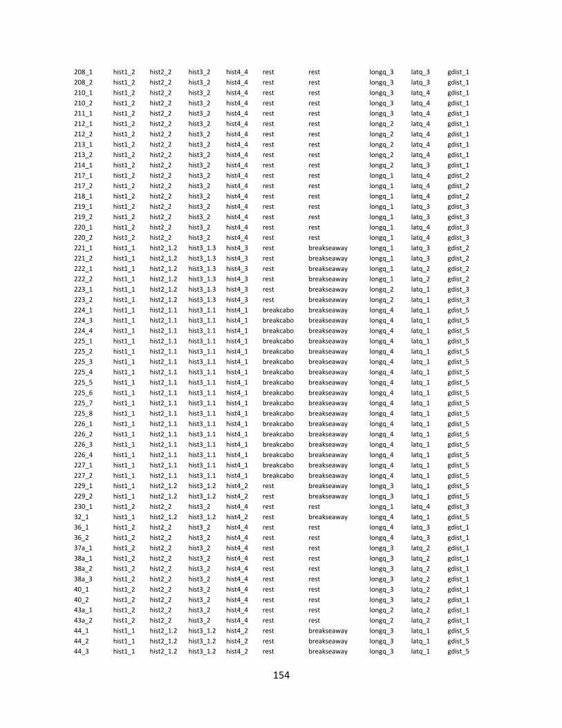
154

208_1 hist1_2 hist2_2 hist3_2 hist4_4 rest rest longq_3 latq_3 gdist_1

208_2 hist1_2 hist2_2 hist3_2 hist4_4 rest rest longq_3 latq_3 gdist_1

210_1 hist1_2 hist2_2 hist3_2 hist4_4 rest rest longq_3 latq_4 gdist_1

210_2 hist1_2 hist2_2 hist3_2 hist4_4 rest rest longq_3 latq_4 gdist_1

211_1 hist1_2 hist2_2 hist3_2 hist4_4 rest rest longq_3 latq_4 gdist_1

212_1 hist1_2 hist2_2 hist3_2 hist4_4 rest rest longq_2 latq_4 gdist_1

212_2 hist1_2 hist2_2 hist3_2 hist4_4 rest rest longq_2 latq_4 gdist_1

213_1 hist1_2 hist2_2 hist3_2 hist4_4 rest rest longq_2 latq_4 gdist_1

213_2 hist1_2 hist2_2 hist3_2 hist4_4 rest rest longq_2 latq_4 gdist_1

214_1 hist1_2 hist2_2 hist3_2 hist4_4 rest rest longq_2 latq_3 gdist_1

217_1 hist1_2 hist2_2 hist3_2 hist4_4 rest rest longq_1 latq_4 gdist_2

217_2 hist1_2 hist2_2 hist3_2 hist4_4 rest rest longq_1 latq_4 gdist_2

218_1 hist1_2 hist2_2 hist3_2 hist4_4 rest rest longq_1 latq_4 gdist_2

219_1 hist1_2 hist2_2 hist3_2 hist4_4 rest rest longq_1 latq_3 gdist_3

219_2 hist1_2 hist2_2 hist3_2 hist4_4 rest rest longq_1 latq_3 gdist_3

220_1 hist1_2 hist2_2 hist3_2 hist4_4 rest rest longq_1 latq_4 gdist_3

220_2 hist1_2 hist2_2 hist3_2 hist4_4 rest rest longq_1 latq_4 gdist_3

221_1 hist1_1 hist2_1.2 hist3_1.3 hist4_3 rest breakseaway longq_1 latq_3 gdist_2

221_2 hist1_1 hist2_1.2 hist3_1.3 hist4_3 rest breakseaway longq_1 latq_3 gdist_2

222_1 hist1_1 hist2_1.2 hist3_1.3 hist4_3 rest breakseaway longq_1 latq_2 gdist_2

222_2 hist1_1 hist2_1.2 hist3_1.3 hist4_3 rest breakseaway longq_1 latq_2 gdist_2

223_1 hist1_1 hist2_1.2 hist3_1.3 hist4_3 rest breakseaway longq_2 latq_1 gdist_3

223_2 hist1_1 hist2_1.2 hist3_1.3 hist4_3 rest breakseaway longq_2 latq_1 gdist_3

224_1 hist1_1 hist2_1.1 hist3_1.1 hist4_1 breakcabo breakseaway longq_4 latq_1 gdist_5

224_3 hist1_1 hist2_1.1 hist3_1.1 hist4_1 breakcabo breakseaway longq_4 latq_1 gdist_5

224_4 hist1_1 hist2_1.1 hist3_1.1 hist4_1 breakcabo breakseaway longq_4 latq_1 gdist_5

225_1 hist1_1 hist2_1.1 hist3_1.1 hist4_1 breakcabo breakseaway longq_4 latq_1 gdist_5

225_2 hist1_1 hist2_1.1 hist3_1.1 hist4_1 breakcabo breakseaway longq_4 latq_1 gdist_5

225_3 hist1_1 hist2_1.1 hist3_1.1 hist4_1 breakcabo breakseaway longq_4 latq_1 gdist_5

225_4 hist1_1 hist2_1.1 hist3_1.1 hist4_1 breakcabo breakseaway longq_4 latq_1 gdist_5

225_5 hist1_1 hist2_1.1 hist3_1.1 hist4_1 breakcabo breakseaway longq_4 latq_1 gdist_5

225_6 hist1_1 hist2_1.1 hist3_1.1 hist4_1 breakcabo breakseaway longq_4 latq_1 gdist_5

225_7 hist1_1 hist2_1.1 hist3_1.1 hist4_1 breakcabo breakseaway longq_4 latq_1 gdist_5

225_8 hist1_1 hist2_1.1 hist3_1.1 hist4_1 breakcabo breakseaway longq_4 latq_1 gdist_5

226_1 hist1_1 hist2_1.1 hist3_1.1 hist4_1 breakcabo breakseaway longq_4 latq_1 gdist_5

226_2 hist1_1 hist2_1.1 hist3_1.1 hist4_1 breakcabo breakseaway longq_4 latq_1 gdist_5

226_3 hist1_1 hist2_1.1 hist3_1.1 hist4_1 breakcabo breakseaway longq_4 latq_1 gdist_5

226_4 hist1_1 hist2_1.1 hist3_1.1 hist4_1 breakcabo breakseaway longq_4 latq_1 gdist_5

227_1 hist1_1 hist2_1.1 hist3_1.1 hist4_1 breakcabo breakseaway longq_4 latq_1 gdist_5

227_2 hist1_1 hist2_1.1 hist3_1.1 hist4_1 breakcabo breakseaway longq_4 latq_1 gdist_5

229_1 hist1_1 hist2_1.2 hist3_1.2 hist4_2 rest breakseaway longq_3 latq_1 gdist_5

229_2 hist1_1 hist2_1.2 hist3_1.2 hist4_2 rest breakseaway longq_3 latq_1 gdist_5

230_1 hist1_2 hist2_2 hist3_2 hist4_4 rest rest longq_1 latq_4 gdist_3

32_1 hist1_1 hist2_1.2 hist3_1.2 hist4_2 rest breakseaway longq_4 latq_1 gdist_5

36_1 hist1_2 hist2_2 hist3_2 hist4_4 rest rest longq_4 latq_3 gdist_1

36_2 hist1_2 hist2_2 hist3_2 hist4_4 rest rest longq_4 latq_3 gdist_1

37a_1 hist1_2 hist2_2 hist3_2 hist4_4 rest rest longq_3 latq_2 gdist_1

38a_1 hist1_2 hist2_2 hist3_2 hist4_4 rest rest longq_3 latq_2 gdist_1

38a_2 hist1_2 hist2_2 hist3_2 hist4_4 rest rest longq_3 latq_2 gdist_1

38a_3 hist1_2 hist2_2 hist3_2 hist4_4 rest rest longq_3 latq_2 gdist_1

40_1 hist1_2 hist2_2 hist3_2 hist4_4 rest rest longq_3 latq_2 gdist_1

40_2 hist1_2 hist2_2 hist3_2 hist4_4 rest rest longq_3 latq_2 gdist_1

43a_1 hist1_2 hist2_2 hist3_2 hist4_4 rest rest longq_2 latq_2 gdist_1

43a_2 hist1_2 hist2_2 hist3_2 hist4_4 rest rest longq_2 latq_2 gdist_1

44_1 hist1_1 hist2_1.2 hist3_1.2 hist4_2 rest breakseaway longq_3 latq_1 gdist_5

44_2 hist1_1 hist2_1.2 hist3_1.2 hist4_2 rest breakseaway longq_3 latq_1 gdist_5

44_3 hist1_1 hist2_1.2 hist3_1.2 hist4_2 rest breakseaway longq_3 latq_1 gdist_5

155

47a_1 hist1_2 hist2_2 hist3_2 hist4_4 rest rest longq_3 latq_2 gdist_2

49_1 hist1_1 hist2_1.2 hist3_1.2 hist4_2 rest breakseaway longq_3 latq_1 gdist_5

49_2 hist1_1 hist2_1.2 hist3_1.2 hist4_2 rest breakseaway longq_3 latq_1 gdist_5

50_1 hist1_1 hist2_1.2 hist3_1.2 hist4_2 rest breakseaway longq_3 latq_1 gdist_5

50_2 hist1_1 hist2_1.2 hist3_1.2 hist4_2 rest breakseaway longq_3 latq_1 gdist_5

50_3 hist1_1 hist2_1.2 hist3_1.2 hist4_2 rest breakseaway longq_3 latq_1 gdist_5

51a_3 hist1_2 hist2_2 hist3_2 hist4_4 rest rest longq_4 latq_2 gdist_3

53a_2 hist1_2 hist2_2 hist3_2 hist4_4 rest rest longq_4 latq_1 gdist_3

56a_1 hist1_2 hist2_2 hist3_2 hist4_4 rest rest longq_4 latq_1 gdist_4

56a_2 hist1_2 hist2_2 hist3_2 hist4_4 rest rest longq_4 latq_1 gdist_4

66_1 hist1_2 hist2_2 hist3_2 hist4_4 rest rest longq_3 latq_3 gdist_1

66_2 hist1_2 hist2_2 hist3_2 hist4_4 rest rest longq_3 latq_3 gdist_1

74_1 hist1_2 hist2_2 hist3_2 hist4_4 rest rest longq_2 latq_4 gdist_1

74_2 hist1_2 hist2_2 hist3_2 hist4_4 rest rest longq_2 latq_4 gdist_1

84_1 hist1_1 hist2_1.2 hist3_1.3 hist4_3 rest breakseaway longq_2 latq_1 gdist_4

84_2 hist1_1 hist2_1.2 hist3_1.3 hist4_3 rest breakseaway longq_2 latq_1 gdist_4

88_1 hist1_2 hist2_2 hist3_2 hist4_4 rest rest longq_2 latq_4 gdist_1

93_1 hist1_1 hist2_1.2 hist3_1.3 hist4_3 rest breakseaway longq_2 latq_2 gdist_2

93_2 hist1_1 hist2_1.2 hist3_1.3 hist4_3 rest breakseaway longq_2 latq_2 gdist_2

97_1 hist1_2 hist2_2 hist3_2 hist4_4 rest rest longq_1 latq_4 gdist_4

97_2 hist1_2 hist2_2 hist3_2 hist4_4 rest rest longq_1 latq_4 gdist_4

L1 hist1_2 hist2_2 hist3_2 hist4_4 rest rest longq_4 latq_1 gdist_5

L10 hist1_2 hist2_2 hist3_2 hist4_4 rest rest longq_2 latq_3 gdist_1

L11 hist1_1 hist2_1.2 hist3_1.3 hist4_3 rest breakseaway longq_2 latq_2 gdist_2

L12 hist1_2 hist2_2 hist3_2 hist4_4 rest rest longq_2 latq_3 gdist_1

L13 hist1_2 hist2_2 hist3_2 hist4_4 rest rest longq_2 latq_2 gdist_2

L14 hist1_2 hist2_2 hist3_2 hist4_4 rest rest longq_2 latq_2 gdist_2

L15 hist1_2 hist2_2 hist3_2 hist4_4 rest rest longq_2 latq_2 gdist_2

L16 hist1_2 hist2_2 hist3_2 hist4_4 rest rest longq_2 latq_1 gdist_2

L17 hist1_2 hist2_2 hist3_2 hist4_4 rest rest longq_2 latq_2 gdist_2

L18 hist1_2 hist2_2 hist3_2 hist4_4 rest rest longq_2 latq_1 gdist_2

L19 hist1_2 hist2_2 hist3_2 hist4_4 rest rest longq_2 latq_1 gdist_2

L2 hist1_2 hist2_2 hist3_2 hist4_4 rest rest longq_2 latq_2 gdist_2

L20 hist1_2 hist2_2 hist3_2 hist4_4 rest rest longq_2 latq_2 gdist_2

L21 hist1_1 hist2_1.2 hist3_1.3 hist4_3 rest breakseaway longq_2 latq_2 gdist_2

L22 hist1_1 hist2_1.2 hist3_1.3 hist4_3 rest breakseaway longq_2 latq_2 gdist_2

L3 hist1_2 hist2_2 hist3_2 hist4_4 rest rest longq_2 latq_2 gdist_1

L4 hist1_2 hist2_2 hist3_2 hist4_4 rest rest longq_3 latq_1 gdist_3

L5 hist1_2 hist2_2 hist3_2 hist4_4 rest rest longq_2 latq_2 gdist_2

L6 hist1_2 hist2_2 hist3_2 hist4_4 rest rest longq_4 latq_2 gdist_3

L7 hist1_2 hist2_2 hist3_2 hist4_4 rest rest longq_2 latq_2 gdist_2

L8 hist1_2 hist2_2 hist3_2 hist4_4 rest rest longq_3 latq_1 gdist_3

L9 hist1_2 hist2_2 hist3_2 hist4_4 rest rest longq_3 latq_1 gdist_3

pser1 out out out out out out out out out

pser2 out out out out out out out out out

pser3 out out out out out out out out out

pser4 out out out out out out out out out

Individual NicheDistQuart Vegetation Ecoregions

102_1 edistq_2 Central Desert Baja California desert

102_2 edistq_2 Central Desert Baja California desert

103_1 edistq_2 Mojave Mojave desert

105_1 edistq_2 Mojave Mojave desert

105_2 edistq_2 Mojave Mojave desert

122_1 edistq_2 Mojave Mojave desert

156

127_1 edistq_2 Central Desert Baja California desert

127_2 edistq_2 Central Desert Baja California desert

129_1 edistq_1 Lower Colorado Desert Sonoran desert

129_2 edistq_1 Lower Colorado Desert Sonoran desert

136_1 edistq_1 Mojave Mojave desert

139_1 edistq_1 Lower Colorado Desert Sonoran desert

141_1 edistq_2 Mojave Mojave desert

141_2 edistq_2 Mojave Mojave desert

188_1 edistq_2 Mojave Mojave desert

188_2 edistq_2 Mojave Mojave desert

194_1 edistq_1 Chihuahuan Desert Chihuahuan desert

194_2 edistq_1 Chihuahuan Desert Chihuahuan desert

195_1 edistq_1 Arizona Upland Sonoran desert

195_2 edistq_1 Arizona Upland Sonoran desert

201_1 edistq_1 Chihuahuan Desert Chihuahuan desert

201_2 edistq_1 Chihuahuan Desert Chihuahuan desert

202_1 edistq_3 Arizona Mountains Forest Arizona Mountains forests

202_2 edistq_3 Arizona Mountains Forest Arizona Mountains forests

203_1 edistq_2 Arizona Mountains Forest Arizona Mountains forests

203_2 edistq_2 Arizona Mountains Forest Arizona Mountains forests

207_1 edistq_1 Arizona Upland Sonoran desert

208_1 edistq_1 Arizona Upland Sonoran desert

208_2 edistq_1 Arizona Upland Sonoran desert

210_1 edistq_1 Arizona Upland Sonoran desert

210_2 edistq_1 Arizona Upland Sonoran desert

211_1 edistq_1 Arizona Mountains Forest Arizona Mountains forests

212_1 edistq_2 Arizona Upland Sonoran desert

212_2 edistq_2 Arizona Upland Sonoran desert

213_1 edistq_1 Arizona Upland Sonoran desert

213_2 edistq_1 Arizona Upland Sonoran desert

214_1 edistq_1 Lower Colorado Desert Sonoran desert

217_1 edistq_2 Lower Colorado Desert Sonoran desert

217_2 edistq_2 Lower Colorado Desert Sonoran desert

218_1 edistq_1 Lower Colorado Desert Sonoran desert

219_1 edistq_2 Lower Colorado Desert Sonoran desert

219_2 edistq_2 Lower Colorado Desert Sonoran desert

220_1 edistq_1 Mojave Mojave desert

220_2 edistq_1 Mojave Mojave desert

221_1 edistq_2 Chaparral California coastal sage and chaparral

221_2 edistq_2 Chaparral California coastal sage and chaparral

222_1 edistq_2 Central Desert Baja California desert

222_2 edistq_2 Central Desert Baja California desert

223_1 edistq_2 Central Desert Baja California desert

223_2 edistq_2 Central Desert Baja California desert

224_1 edistq_4 Gulf Coast San Lucan xeric scrub

224_3 edistq_4 Gulf Coast San Lucan xeric scrub

224_4 edistq_4 Gulf Coast San Lucan xeric scrub

225_1 edistq_3 Sarcocaulescent Shrubland San Lucan xeric scrub

225_2 edistq_3 Sarcocaulescent Shrubland San Lucan xeric scrub

225_3 edistq_3 Sarcocaulescent Shrubland San Lucan xeric scrub

225_4 edistq_3 Sarcocaulescent Shrubland San Lucan xeric scrub

225_5 edistq_3 Sarcocaulescent Shrubland San Lucan xeric scrub

225_6 edistq_3 Sarcocaulescent Shrubland San Lucan xeric scrub

225_7 edistq_3 Sarcocaulescent Shrubland San Lucan xeric scrub

225_8 edistq_3 Sarcocaulescent Shrubland San Lucan xeric scrub

226_1 edistq_4 Sarcocaulescent Shrubland San Lucan xeric scrub

226_2 edistq_4 Sarcocaulescent Shrubland San Lucan xeric scrub

157

226_3 edistq_4 Sarcocaulescent Shrubland San Lucan xeric scrub

226_4 edistq_4 Sarcocaulescent Shrubland San Lucan xeric scrub

227_1 edistq_4 Sarcocaulescent Shrubland San Lucan xeric scrub

227_2 edistq_4 Sarcocaulescent Shrubland San Lucan xeric scrub

229_1 edistq_3 Gulf Coast Gulf of California xeric scrub

229_2 edistq_3 Gulf Coast Gulf of California xeric scrub

230_1 edistq_2 Mojave Mojave desert

32_1 edistq_4 Gulf Coast Gulf of California xeric scrub

36_1 edistq_1 Arizona Upland Sonoran desert

36_2 edistq_1 Arizona Upland Sonoran desert

37a_1 edistq_2 Chihuahuan Desert Chihuahuan desert

38a_1 edistq_1 Arizona Upland Sonoran desert

38a_2 edistq_1 Arizona Upland Sonoran desert

38a_3 edistq_1 Arizona Upland Sonoran desert

40_1 edistq_1 Chihuahuan Desert Chihuahuan desert

40_2 edistq_1 Chihuahuan Desert Chihuahuan desert

43a_1 edistq_1 Lower Colorado Desert Sonoran desert

43a_2 edistq_1 Lower Colorado Desert Sonoran desert

44_1 edistq_3 Magdalena Plains Baja California desert

44_2 edistq_3 Magdalena Plains Baja California desert

44_3 edistq_3 Magdalena Plains Baja California desert

47a_1 edistq_2 Gulf Coast Sonoran desert

49_1 edistq_3 Magdalena Plains Baja California desert

49_2 edistq_3 Magdalena Plains Baja California desert

50_1 edistq_4 Magdalena Plains Baja California desert

50_2 edistq_4 Magdalena Plains Baja California desert

50_3 edistq_4 Magdalena Plains Baja California desert

51a_3 edistq_2 Plains of Sonora Sonoran desert

53a_2 edistq_3 Sonoran thornscrub Sonoran-Sinaloan transition subtropical dry forest

56a_1 edistq_4 Sonoran thornscrub Sonoran-Sinaloan transition subtropical dry forest

56a_2 edistq_4 Sonoran thornscrub Sonoran-Sinaloan transition subtropical dry forest

66_1 edistq_1 Arizona Upland Sonoran desert

66_2 edistq_1 Arizona Upland Sonoran desert

74_1 edistq_1 Arizona Upland Sonoran desert

74_2 edistq_1 Arizona Upland Sonoran desert

84_1 edistq_3 Vizcaino Desert Baja California desert

84_2 edistq_3 Vizcaino Desert Baja California desert

88_1 edistq_1 Lower Colorado Desert Sonoran desert

93_1 edistq_2 Central Desert Baja California desert

93_2 edistq_2 Central Desert Baja California desert

97_1 edistq_3 Mojave Mojave desert

97_2 edistq_3 Mojave Mojave desert

L1 edistq_3 Sonoran thornscrub Sonoran-Sinaloan transition subtropical dry forest

L10 edistq_1 Lower Colorado Desert Sonoran desert

L11 edistq_2 Gulf Coast Gulf of California xeric scrub

L12 edistq_1 Lower Colorado Desert Sonoran desert

L13 edistq_1 Gulf Coast Sonoran desert

L14 edistq_1 Gulf Coast Sonoran desert

L15 edistq_1 Gulf Coast Sonoran desert

L16 edistq_2 Gulf Coast Sonoran desert

L17 edistq_1 Gulf Coast Sonoran desert

L18 edistq_2 Gulf Coast Sonoran desert

L19 edistq_2 Gulf Coast Sonoran desert

L2 edistq_1 Gulf Coast Sonoran desert

L20 edistq_1 Gulf Coast Sonoran desert

L21 edistq_2 Gulf Coast Gulf of California xeric scrub

L22 edistq_2 Gulf Coast Gulf of California xeric scrub

158

L3 edistq_1 Gulf Coast Sonoran desert

L4 edistq_4 Gulf Coast Sonoran desert

L5 edistq_1 Gulf Coast Sonoran desert

L6 edistq_2 Chihuahuan Desert Chihuahuan desert

L7 edistq_1 Gulf Coast Sonoran desert

L8 edistq_4 Gulf Coast Sonoran desert

L9 edistq_4 Gulf Coast Sonoran desert

pser1 out out out

pser2 out out out

pser3 out out out

pser4 out out out

Individual DispYearQuart DispWinterQuart AltQuart Host Genera Null

102_1 dispovq_3 dispwinterq_2 altq_2 Prosopis glandulosa Prosopis in

102_2 dispovq_3 dispwinterq_2 altq_2 Prosopis glandulosa Prosopis in

103_1 dispovq_2 dispwinterq_2 altq_3 Acacia greggii Acacia in

105_1 dispovq_2 dispwinterq_3 altq_3 Acacia greggii Acacia in

105_2 dispovq_2 dispwinterq_3 altq_3 Acacia greggii Acacia in

122_1 dispovq_1 dispwinterq_2 altq_2 Acacia greggii Acacia in

127_1 dispovq_2 dispwinterq_2 altq_2 Prosopis glandulosa Prosopis in

127_2 dispovq_2 dispwinterq_2 altq_2 Prosopis glandulosa Prosopis in

129_1 dispovq_3 dispwinterq_3 altq_2 Olneya tesota Olneya in

129_2 dispovq_3 dispwinterq_3 altq_2 Olneya tesota Olneya in

136_1 dispovq_2 dispwinterq_2 altq_3 Prosopis velutina Prosopis in

139_1 dispovq_2 dispwinterq_3 altq_1 Prosopis glandulosa Prosopis in

141_1 dispovq_3 dispwinterq_2 altq_2 Prosopis velutina Prosopis in

141_2 dispovq_3 dispwinterq_2 altq_2 Prosopis velutina Prosopis in

188_1 dispovq_2 dispwinterq_3 altq_2 Acacia greggii Acacia in

188_2 dispovq_2 dispwinterq_3 altq_2 Acacia greggii Acacia in

194_1 dispovq_4 dispwinterq_4 altq_3 Acacia greggii Acacia in

194_2 dispovq_4 dispwinterq_4 altq_3 Acacia greggii Acacia in

195_1 dispovq_3 dispwinterq_4 altq_2 Prosopis velutina Prosopis in

195_2 dispovq_3 dispwinterq_4 altq_2 Prosopis velutina Prosopis in

201_1 dispovq_3 dispwinterq_3 altq_2 Prosopis velutina Prosopis in

201_2 dispovq_3 dispwinterq_3 altq_2 Prosopis velutina Prosopis in

202_1 dispovq_4 dispwinterq_4 altq_4 Acacia greggii Acacia in

202_2 dispovq_4 dispwinterq_4 altq_4 Acacia greggii Acacia in

203_1 dispovq_3 dispwinterq_4 altq_3 Prosopis velutina Prosopis in

203_2 dispovq_3 dispwinterq_4 altq_3 Prosopis velutina Prosopis in

207_1 dispovq_2 dispwinterq_3 altq_2 Prosopis velutina Prosopis in

208_1 dispovq_3 dispwinterq_4 altq_3 Prosopis velutina Prosopis in

208_2 dispovq_3 dispwinterq_4 altq_3 Prosopis velutina Prosopis in

210_1 dispovq_3 dispwinterq_3 altq_2 Prosopis velutina Prosopis in

210_2 dispovq_3 dispwinterq_3 altq_2 Prosopis velutina Prosopis in

211_1 dispovq_3 dispwinterq_4 altq_3 Acacia greggii Acacia in

212_1 dispovq_3 dispwinterq_3 altq_3 Acacia greggii Acacia in

212_2 dispovq_3 dispwinterq_3 altq_3 Acacia greggii Acacia in

213_1 dispovq_3 dispwinterq_3 altq_2 Acacia greggii Acacia in

213_2 dispovq_3 dispwinterq_3 altq_2 Acacia greggii Acacia in

214_1 dispovq_3 dispwinterq_3 altq_2 Cercidium floridum Cercidium in

217_1 dispovq_2 dispwinterq_3 altq_1 Prosopis velutina Prosopis in

217_2 dispovq_2 dispwinterq_3 altq_1 Prosopis velutina Prosopis in

218_1 dispovq_3 dispwinterq_3 altq_2 Cercidium floridum Cercidium in

219_1 dispovq_2 dispwinterq_3 altq_1 Prosopis glandulosa Prosopis in

219_2 dispovq_2 dispwinterq_3 altq_1 Prosopis glandulosa Prosopis in

159

220_1 dispovq_3 dispwinterq_4 altq_2 Acacia greggii Acacia in

220_2 dispovq_3 dispwinterq_4 altq_2 Acacia greggii Acacia in

221_1 dispovq_3 dispwinterq_4 altq_2 Acacia greggii Acacia in

221_2 dispovq_3 dispwinterq_4 altq_2 Acacia greggii Acacia in

222_1 dispovq_3 dispwinterq_2 altq_2 Prosopis glandulosa Prosopis in

222_2 dispovq_3 dispwinterq_2 altq_2 Prosopis glandulosa Prosopis in

223_1 dispovq_1 dispwinterq_2 altq_1 Prosopis glandulosa Prosopis in

223_2 dispovq_1 dispwinterq_2 altq_1 Prosopis glandulosa Prosopis in

224_1 dispovq_2 dispwinterq_2 altq_1 Cercidium floridum Cercidium in

224_3 dispovq_2 dispwinterq_2 altq_1 Cercidium floridum Cercidium in

224_4 dispovq_2 dispwinterq_2 altq_1 Cercidium floridum Cercidium in

225_1 dispovq_1 dispwinterq_2 altq_1 Prosopis velutina Prosopis in

225_2 dispovq_1 dispwinterq_2 altq_1 Prosopis velutina Prosopis in

225_3 dispovq_1 dispwinterq_2 altq_1 Prosopis velutina Prosopis in

225_4 dispovq_1 dispwinterq_2 altq_1 Prosopis velutina Prosopis in

225_5 dispovq_1 dispwinterq_2 altq_1 Prosopis velutina Prosopis in

225_6 dispovq_1 dispwinterq_2 altq_1 Prosopis velutina Prosopis in

225_7 dispovq_1 dispwinterq_2 altq_1 Prosopis velutina Prosopis in

225_8 dispovq_1 dispwinterq_2 altq_1 Prosopis velutina Prosopis in

226_1 dispovq_2 dispwinterq_2 altq_1 Olneya tesota Olneya in

226_2 dispovq_2 dispwinterq_2 altq_1 Olneya tesota Olneya in

226_3 dispovq_2 dispwinterq_2 altq_1 Olneya tesota Olneya in

226_4 dispovq_2 dispwinterq_2 altq_1 Olneya tesota Olneya in

227_1 dispovq_2 dispwinterq_2 altq_1 Acacia occidentalis Acacia in

227_2 dispovq_2 dispwinterq_2 altq_1 Acacia occidentalis Acacia in

229_1 dispovq_2 dispwinterq_2 altq_1 Prosopis glandulosa Prosopis in

229_2 dispovq_2 dispwinterq_2 altq_1 Prosopis glandulosa Prosopis in

230_1 dispovq_3 dispwinterq_2 altq_3 Acacia greggii Acacia in

32_1 dispovq_2 dispwinterq_2 altq_1 Prosopis velutina Prosopis in

36_1 dispovq_3 dispwinterq_4 altq_2 Prosopis articulata Prosopis in

36_2 dispovq_3 dispwinterq_4 altq_2 Prosopis articulata Prosopis in

37a_1 dispovq_1 dispwinterq_1 altq_2 Cercidium microphyllum Cercidium in

38a_1 dispovq_1 dispwinterq_1 altq_2 Prosopis velutina Prosopis in

38a_2 dispovq_1 dispwinterq_1 altq_2 Prosopis velutina Prosopis in

38a_3 dispovq_1 dispwinterq_1 altq_2 Prosopis velutina Prosopis in

40_1 dispovq_3 dispwinterq_4 altq_3 Acacia greggii Acacia in

40_2 dispovq_3 dispwinterq_4 altq_3 Acacia greggii Acacia in

43a_1 dispovq_3 dispwinterq_4 altq_2 Prosopis velutina Prosopis in

43a_2 dispovq_3 dispwinterq_4 altq_2 Prosopis velutina Prosopis in

44_1 dispovq_2 dispwinterq_2 altq_1 Prosopis glandulosa Prosopis in

44_2 dispovq_2 dispwinterq_2 altq_1 Prosopis glandulosa Prosopis in

44_3 dispovq_2 dispwinterq_2 altq_1 Prosopis glandulosa Prosopis in

47a_1 dispovq_1 dispwinterq_2 altq_1 Prosopis velutina Prosopis in

49_1 dispovq_1 dispwinterq_2 altq_1 Prosopis velutina Prosopis in

49_2 dispovq_1 dispwinterq_2 altq_1 Prosopis velutina Prosopis in

50_1 dispovq_2 dispwinterq_2 altq_1 Prosopis velutina Prosopis in

50_2 dispovq_2 dispwinterq_2 altq_1 Prosopis velutina Prosopis in

50_3 dispovq_2 dispwinterq_2 altq_1 Prosopis velutina Prosopis in

51a_3 dispovq_1 dispwinterq_1 altq_1 Prosopis velutina Prosopis in

53a_2 dispovq_1 dispwinterq_2 altq_2 Prosopis velutina Prosopis in

56a_1 dispovq_1 dispwinterq_2 altq_2 Prosopis velutina Prosopis in

56a_2 dispovq_1 dispwinterq_2 altq_2 Prosopis velutina Prosopis in

66_1 dispovq_3 dispwinterq_3 altq_2 Prosopis velutina Prosopis in

66_2 dispovq_3 dispwinterq_3 altq_2 Prosopis velutina Prosopis in

74_1 dispovq_3 dispwinterq_3 altq_2 Cercidium microphyllum Cercidium in

74_2 dispovq_3 dispwinterq_3 altq_2 Cercidium microphyllum Cercidium in

84_1 dispovq_1 dispwinterq_1 altq_1 Prosopis glandulosa Prosopis in

160

84_2 dispovq_1 dispwinterq_1 altq_1 Prosopis glandulosa Prosopis in

88_1 dispovq_3 dispwinterq_3 altq_2 Cercidium microphyllum Cercidium in

93_1 dispovq_2 dispwinterq_1 altq_2 Acacia greggii Acacia in

93_2 dispovq_2 dispwinterq_1 altq_2 Acacia greggii Acacia in

97_1 dispovq_2 dispwinterq_3 altq_2 Prosopis velutina Prosopis in

97_2 dispovq_2 dispwinterq_3 altq_2 Prosopis velutina Prosopis in

L1 dispovq_1 dispwinterq_1 altq_1 Cercidium praecox Cercidium in

L10 dispovq_3 dispwinterq_2 altq_1 Cercidium floridum Cercidium in

L11 dispovq_2 dispwinterq_2 altq_1 Acacia greggii Acacia in

L12 dispovq_3 dispwinterq_3 altq_1 Olneya tesota Olneya in

L13 dispovq_1 dispwinterq_2 altq_1 Larrea tridentada Larrea in

L14 dispovq_2 dispwinterq_2 altq_1 Olneya tesota Olneya in

L15 dispovq_2 dispwinterq_2 altq_2 Olneya tesota Olneya in

L16 dispovq_2 dispwinterq_2 altq_1 Prosopis velutina Prosopis in

L17 dispovq_2 dispwinterq_2 altq_2 Prosopis velutina Prosopis in

L18 dispovq_2 dispwinterq_2 altq_1 Prosopis velutina Prosopis in

L19 dispovq_2 dispwinterq_2 altq_1 Olneya tesota Olneya in

L2 dispovq_2 dispwinterq_2 altq_1 Olneya tesota Olneya in

L20 dispovq_2 dispwinterq_2 altq_1 Acacia greggii Acacia in

L21 dispovq_2 dispwinterq_2 altq_1 Cercidium microphyllum Cercidium in

L22 dispovq_2 dispwinterq_2 altq_1 Acacia greggii Acacia in

L3 dispovq_2 dispwinterq_2 altq_1 Cercidium floridum Cercidium in

L4 dispovq_2 dispwinterq_2 altq_1 Prosopis glandulosa Prosopis in

L5 dispovq_2 dispwinterq_2 altq_1 Olneya tesota Olneya in

L6 dispovq_3 dispwinterq_3 altq_3 Prosopis velutina Prosopis in

L7 dispovq_2 dispwinterq_2 altq_1 Acacia greggii Acacia in

L8 dispovq_2 dispwinterq_2 altq_1 Prosopis velutina Prosopis in

L9 dispovq_2 dispwinterq_2 altq_1 Acacia greggii Acacia in

pser1 out out out out out out

pser2 out out out out out out

pser3 out out out out out out

pser4 out out out out out out

161

Appendix 4.2. Methods to obtain the layers on the historical, ecological, and geographic

conditions used for population partitioning in the Bayesian coalescent analysis.

Historical vicariant events—Following Riddle et al. (2000) and Garrick et al. (2009)

we draw lines and polygons in ArcMap 10 that correspond to the marine transgression

forming the Gulf of California and the trans-peninsular seaway forming the Isthmus of La

Paz (line running southwest-northeast at approximately long -110.483°, lat 23.923°) and

the mid-peninsular seaway break in central Vizcaino region (long -113.082°, lat 27.370°)

across the Baja California Peninsula. The areas separated by these breaks were used to

annotate the geographic correspondence of the sampled individuals in the categories

described in Table 1.

Vegetation and ecoregional regionalization—We followed Shreve (1951) original

regionalization of the Sonoran Desert vegetation and its modified regionalization only for

Baja California Peninsula following González-Abraham et al. (2010). We modified the

contour of the WWF ecoregions (Olson et al. 2001) to match the contour of the areas

depicted by Shreve and we added the polygons already available by González-Abraham et

al. (2010). Our second alternative of regionalization was following the WWF ecoregions

based on the shapefile available online (http://worldwildlife.org/publications/terrestrial-

ecoregions-of-the-world). The areas resulting in each regionalization are in Table 1.

Elevation—We reclassified in quartiles the elevation layer at 1 km spatial

resolution available from WoldClim (http://www.worldclim.org) and assigned values 1-4

to sampled individuals depending on the quartile they fell given their spatial location.

162

Longitude and latitude—The coordinates of the sampled individuals were divided

in quartiles for latitude and longitude and were assigned a value of 1-4 accordingly.

Distance to geographic range center—This distance is a measure of centrality

with respect to the overall geographic range of the species. We obtained the geographic

centroid of the polygon defining the geographic range of the species, and from this point

we calculated the Euclidean distance to every other point in the geography. These

distances were reclassified from 1-4 according to their corresponding quartile, and these

values were then assigned to the sampled individuals depending on their geographic

position. More details on how to calculate this distance can be found in Lira-Noriega &

Manthey (2014).

Distance to ecological niche centroid—This distance is a measure of

environmental centrality for the species using climatic variables. To obtain the centroid,

we extracted values of the 19 bioclimatic variables at 2.5’ from WorldClim

(http://www.worldclim.org) on the thresholded climatic niche of the species using

Maxent (see main document for details) and estimated vector of means for each variable.

Then, from the vector of means, we calculated Euclidean distances to every other point in

the area of study for the same 19 variables. These values were classified in four according

to their quartile and projected on geographic space, and each sampled individual was

assigned the value that corresponds to their location. More details on how to calculate

this distance can be found in Lira-Noriega & Manthey (2014).

163

Host species and genera—We retrieved the host species for each of the sampled

individuals using the specimens and notes collected during fieldwork, and from the

information in the label in the case of loan specimens.

Year-round and wintertime dispersers suitability—We overlaid the thresholded

suitability models of bird species known to be either specialists or generalists according to

their year-round or wintertime distributions from Lira-Noriega & Peterson (accepted),

and the resulting richness values in the area of study were divided in quartiles and each

sampled individual was assigned a value 1-4 according to their geographic location.

164

Appendix 4.3 Packrat midden localities from western North America with hosts and

mistletoe macrofossil information.

Region Locality Longitude Latitude Macrofossils species (years ago) Reference

Sonoran Desert

Eagle Eye Mountain

-113.177691 33.88868 Acacia greggii (10440-4040), Acacia constricta (3300), Cercidium floridum (6400), Cercidium microphyllum (4500), Larrea tridentata (6400), Prosopis velutina (4500), Phoradendron californicum (6400)

McAuliffe&Van Devender (1998) Palaeogeography, Palaeoclimatology, Palaeoecology 141:253-275

Sonoran Desert

Waterman Mts.

-111.477063 32.3595 Acacia greggii (13000-5000), Cercidium floridum (8000-6500), Cercidium microphyllum (4000), Larrea tridentata (6000), Prosopis velutina (13000)

McAuliffe&Van Devender (1998) Palaeogeography, Palaeoclimatology, Palaeoecology 141:253-275

Sonoran Desert

Puerto Blancon Mts.

-112.857987 32.00451 Acacia greggii (11000-5000), Cercidium floridum (10000-5000), Cercidium microphyllum (6500), Larrea tridentata (8000), Prosopis velutina (11000-5000), Phoradendron californicum (6400)

McAuliffe&Van Devender (1998) Palaeogeography, Palaeoclimatology, Palaeoecology 141:253-275

Sonoran Desert

Hornaday Mts.

-113.6 31.98333

Sonoran Desert

Tinajas Altas Mts.

-114.075 32.3 Acacia greggii (43000, 11000-), Olneya tesota (9700?, 4000-), Cercidium floridum (8900-8500, 4000), Cercidium microphyllum (2000-)

Van Devender 1990 chp 8 in Betancourt et al. eds (1990)

Sonoran Desert

Picacho Peak, CA

-114.641667 32.95 Acacia greggii (11000-8000), Olneya tesota (500-)

Van Devender 1990 chp 8 in Betancourt et al. eds (1990)

Sonoran Desert

Whipple Mts. -114.391667 34.24167 Acacia greggii (12500-), Cercidium floridum (4300, present)

Van Devender 1990 chp 8 in Betancourt et al. eds (1990)

Chihuahuan Desert

Maravillas Canyon Cave

-102.833333 29.55 Acacia graggii (9000-), Prosopis glandulosa (10000-)

Van Devender 1990 chp 7 in Betancourt et al. eds (1990)

Chihuahuan Desert

Rio Grande Village area

-102.966667, -103.016667

29.225 Acacia graggii (5500-), Prosopis glandulosa (11400-)

Van Devender 1990 chp 7 in Betancourt et al. eds (1990)

Chihuahuan Desert

Hueco Mountains

-105.983333, -106.15

31.8 Prosopis glandulosa (11000-) Van Devender 1990 chp 7 in Betancourt et al. eds (1990)

Big Bend, Texas (LGM refugia)

Big Bend (wide region)

-103.1 29.53333 Larrea tridentata (from the Chihuahuan desert and its expansion towards the Sonoran)

Van Devender 1990 chp 7 in Betancourt et al. eds (1990)

165

Appendix 4.4 Model evaluation.

Model Area 0 Area 1 Prob. presence Trials Successes P value

Acacia greggii 51610 87723 0.629592415 100 91 P < 0.001

Cercidium floridum 47971 17015 0.261825624 99 78 P < 0.001

Cercidium microphyllum 22738 17744 0.438318265 100 91 P < 0.001

Prosopis glandulosa 169737 122583 0.419345238 99 79 P < 0.001

Prosopis velutina 121153 17068 0.123483407 100 65 P < 0.001

Phoradendron californicum 52979 24782 0.318694461 100 60 P < 0.001

Phainopepla nitens 206097 84569 0.290949062 100 94 P < 0.001

166

Table S4.1 Results from delimitation of lineages using the ML GMYC method. Both

single- and multiple-threshold favored the delimitation of more than one group (P < 0.05).

However, single threshold was favored due to likely artificial overpartitioned of groups in

the multiple-threshold criterion (see text).

Single Multiple

Likelihood of null model 1358.265 1358.265

Maximum likelihood of GMYC model 1362.186 1366.448

Likelihood ratio 7.842902 (P < 0.05) 16.36765 (P < 0.05)

Number of detected clusters 5 33

Confidence interval 2-23 29-37

Number of ML significant clusters 5 53

Confidence interval 2-32 39-60

167

Table S4.2 Marginal likelihood and Bayes factor of the hypotheses used to test the

phylogenetic relationships of the gene tree without population 225 (see Table 4.1).

Hypotheses are listed in order of importance according to the marginal likelihood. Bayes

factor is estimated with respect to the hypothesis with largest likelihood.

Hypothesis Marginal likelihood 2ln Bayes factor

Historic 4 (subdivision based on major breaks

resulting from geologic vicariant events) -3939.293

Historic 2 (trans-peninsular seaway forming the

Isthmus of La Paz; 3 mya) -3949.728 20.869

Historic 1 (northward transgression forming the Gulf

of California; 3-5 mya) -3958.404 38.222

Latitude (quartiles) -3959.339 40.093

Vegetation (Shreve 1951) -3961.661 44.735

Mid-peninsular seaway break in the central Vizcaino

region -3964.609 50.632

Distance to geographic range center (quartiles) -3965.529 52.472

Ecoregions -3969.383 60.179

Distance to ecological niche centroid (quartiles) -3971.402 64.218

Longitude (quartiles) -3974.747 70.907

Isthmus of La Paz break -3982.316 86.046

Wintertime dispersers suitability (quartiles) -3988.182 97.778

Elevation (quartiles) -3992.386 106.185

Year-round dispersers suitability (quartiles) -3995.294 112.002

Genera -3999.640 120.694

Null hypothesis -3999.703 120.819

Host species -4005.586 132.585

Note: Following Kass and Raftery (1995), the Bayes factor scale of strength of evidence in

favor of one hypothesis is: 0-2 (not worthy of mention), 2-6 (positive), 6-10 (strong), >10

(very strong).

168

Table S4.3 Levels of nucleotide variability per sequenced chloroplast region.

atpH-atpI rpl32-trnL trnQ-rpl16

Sequence length (bp) 632 465 552

Variable positions (bp) 22 23 30

Number of indels 31 20 61

Individuals sequenced (ingroup) 119 124 104

Nucleotide diversity (π) 0.01824 0.01149 0.00844

Haplotype diversity (h) 0.86 0.818 0.763

Tajima's D* (ingroup) -0.93063 (n.s.) -1.05183 (n.s.) -0.26308 (n.s.)

Fu and Li F* (Ingroup) -0.93826 (n.s.) -1.46048 (n.s.) -0.28532 (n.s.)

n.s.: non-statistically significant (P > 0.05).

Haplotype diversity (h) and nucleotide variability (π) suggest similar levels of variability

among regions; tests of neutrality suggest no deviation from neutral variation across

regions. Statistics were calculated using DnaSP v5.10.1 (Librado & Rozas 2009).

Librado P, Rozas J (2009) DnaSP v5: A software for comprehensive analysis of DNA

polymorphism data. Bioinfor 25, 1451 - 1452.

169

Figure S4.1 Phoradendron californicum haplotype network and potential distribution

for mistletoe (inset) and hosts distributions during the LGM (21 kya) according to the

CCSM climate scenario.

Figure S4.1 (A) Phoradendron californicum haplotype network for the three cpDNA concatenated regions colored by host species, excluding haplotypes from clade 4. (B) Potential distribution for mistletoe (inset) and hosts distributions during the LGM (21 kya) according to the CCSM climate scenario, showing geographic locations of most frequent haplotypes and macrofossil localities with mistletoe or hosts. (Supporting Information)

170

Figure S4.2 Haplotype network configuration on concatenated data sets including two

cpDNA regions.

Figure S4.2 Haplotype configuration based on concatenated data sets including two cpDNA regions (atpH-atpI + rpl32-trnL, atpH-atpI + trnQ-rps16, rpl32-trnL + trnQ-rps16). Colors depict the membership established in gene tree reconstruction and GMYC analysis.