speckle and feature motion estimation in...
TRANSCRIPT

in partnership with
Tuathan O'Shea
Speckle and feature motion estimation in ultrasound

Motivation & Research Questions
Intra-fraction motion estimation in RT
Can 3D US speckle tracking accurately estimate prostate displacement
● Is 3D required for the prostate
Can direct US motion estimation remain accurate for long (in vivo liver) sequences
● Ways to improve raw motion estimation (temporal regularisation)

US speckle vs. fiducials3
Cryogel phantom + fiducials
US probeO'Shea et al. Phys. Med. Biol. (2014)

Direct US motion estimate4
Speckle (featureless) – 2D and 3D
1.7 Hz (ultrasound)
0.05 Hz (mean) (x-ray)
sweep

Prostate motion estimation (tracking)5
98.4% of estimates with difference < ± 0.5 mm
+

Motion estimation RMS error6

Prostate motion estimation (gating)7
l RMSE ≤ 0.4 mm for thresholds of 2 mm and 5 mm, All RL motion < 2 mm

Inter-volume correlation8

Is 3D prostate motion estimation required?
9
O'Shea et al. ICCR (2013)
CalypsoTM data from Royal Marsden
“Positioning by prostate markers at the start of the treatment fraction reduced [RL margin to 1.8 mm]” Litzenberg et al. (2005), n = 11
Fraction of time displaced by > 3mm (RL): 1.2% Langen et al. (2008), n = 17
From other studies

Speckle decorrelation10
0 0.1 0.2 0.3 0.4 0.5 0.6 0.7 0.8 0.9 1 1.1 1.20.9
0.91
0.92
0.93
0.94
0.95
0.96
0.97
0.98
0.99
1
1.01
Elevational
input displacement [mm]
inte
rfra
me
co
rre
latio
n
0 0.5 1 1.5 2 2.5 3 3.5 4 4.5 5 5.50.89
0.91
0.93
0.95
0.97
0.99
Elevational decorrelation curve
RL rotate [degs]
AP rotate [degs]
elev. Disp. [mm]
input displacement [mm] / rotation [degs]in
terf
ram
e c
orr
ela
tion
2D imageplane
Tuthill et al. (1998),Houseden et al. (2007)
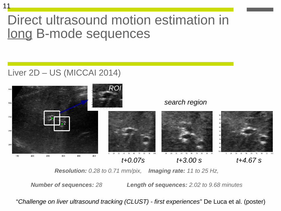
Direct ultrasound motion estimation in long B-mode sequences
Liver 2D – US (MICCAI 2014)
11
Frame 1 Frame 2
Resolution: 0.28 to 0.71 mm/pix, Imaging rate: 11 to 25 Hz,
Number of sequences: 28 Length of sequences: 2.02 to 9.68 minutes
“Challenge on liver ultrasound tracking (CLUST) - first experiences” De Luca et al. (poster)
ROI
search region
t+0.07s t+3.00 s t+4.67 s

Motion estimation errors
False matches
12

Simple temporal regularisation
Correction of initial motion estimation using a-prioir knowledge of motion behaviour (and similarity measure)
13
Errordetection
Motionprediction
Raw motionestimate
Correction
Improvedmotion estimate

ROI update
Fixed versus Hybrid fixed/incremental
14
Fixed ROI
Hybrid fixed/incr.
I[1] I[2]I I[3]I I[N]
I[1] I[2]I I[3]I I[N]...
...

Error detection
Correlation peak plus inter-frame displacement
15
Calculated for SHL = 5 s

Motion prediction16
Linear extrapolation
Linear prediction
Breathing model (Lujan et al. 1999)
where Xt is the predicted displacement at time t, X
t-1and X
t-2 are previous two displacement estimates
without error as determined by error detection algorithm

0.7 0.75 0.8 0.85 0.9 0.95 10
2
4
6
correlation threshold (TVC)
RM
SE
[mm
]
0 0.5 1 1.5 2 2.5 30
1
2
3
4
5
max. inter-frame disp. (TVD) [mm]
RM
SE
[mm
]
Results17
frame
disp
lace
men
t [pi
x.]

1 2 3 4 5 60.0
2.0
4.0
6.0
8.0
10.0
12.0
14.0
Hybrid fixed / incr.; Scanner 2 (MED)
vessel number
dist
an
ce [
mm
]
MICCAI Results
MTE...
18
1 2 3 4 5 6 7 8 90.0
2.0
4.0
6.0
8.0
10.0
Fixed ROI; Scanner 1 (ETH)
mean [mm]
Mean (mean [mm])
max [mm]
vessel number
dist
an
ce [
mm
]
1 2 3 4 5 60.0
2.0
4.0
6.0
8.0
10.0
Fixed ROI; Scanner 2 (MED)
vessel number
dist
an
ce [
mm
]
T. O'Shea, J. Bamber and E. Harris, Medical Image Computing and Computer Assisted Intervention (2014)
Scanner 3

Motion prediction19
Linear extrapolation●
●
Linear prediction●(e.g. Sharp et al. 2004)●
●
Breathing model ●(Lujan et al. 1999)where X
t is the predicted displacement at time t, X
0 is the position at exhale, b is amplitude of breathing, τ
is the breathing period and Ф is the phase.

Motion prediction20
Simulated 15 Hz imaging rate, 5 s SHL
0.5 1 1.50
0.1
0.2
0.3
0.4
0.5
0.6
0.7
0.8
0.9
linear extrapolation
linear prediction
breathing model pred.
prediction length [s]
RM
SE
[mm
]
0.5 1 1.50
1
2
3
4
5
6
linear extrapolation
linear prediction
breathing model pred.
prediction length [s]
ma
xim
um
diff
ere
nce
[mm
]

Results
Results...
21
none (coarse)none (fine)
linear extrap.linear predict.
breathing model
0
0.2
0.4
0.6
0.8
1
1.2vessel 1
vessel 2
regularisation prediction method
2D
RM
SE
[mm
]

0.85 0.9 0.95 1 1.050
5
10
15
normalised threshold value [a.u]
inte
r-fr
am
e fa
lse
po
stiv
es
[%]
0.5 0.55 0.6 0.65 0.7 0.75 0.8 0.85 0.9 0.95 1 1.050
20
40
60
80
100
120
Spatial Correlation
Hist. Correlation
Similarity (Beta = 0.2)
Similarity (Beta = 0.5)
Similarity (Beta = 0.8)
normalised threshold value [a.u]
pe
rce
nta
ge
of i
nte
r-fr
am
e e
rro
rs d
ete
cte
d [%
]
Error detection metric comparison22
(Grey-scale composition)
(Spatial similarity)

Predict – measure - update23
predict
measureupdate
• α and β gains• prediction error, X
error
Benedict and Bordner (1962), Lewis (1984), Morris (1986), Penoyer (1993)
Modified αβ Filter

0.1 0.2 0.3 0.4 0.5 0.6 0.7 0.8 0.9 1 1.10.8
0.9
1
1.1
1.2
1.3
1.4
1.5
β = α^2 / 2 – α
α
2D
RM
SE
[mm
]Modified αβ Filter
24
(Benedict and Bordner 1962)
0.6 1.0similarity0.1
0.9
alph
a
sim = 0.85
α ~ 0.6
0.5 0.55 0.6 0.650.8
0.85
0.9
0.95
1
1.05
1.1
1.15
1.2
1.25
1.3
sim. threshold
2D
RM
SE
[mm
]
Varying GainFixed Gain
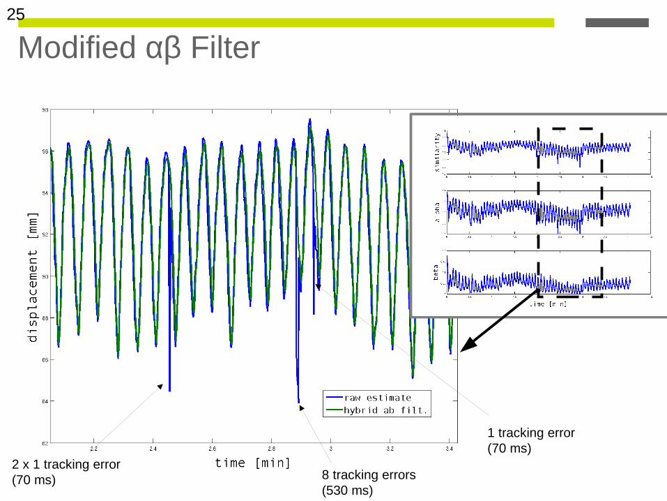
Modified αβ Filter25
2 x 1 tracking error(70 ms) 8 tracking errors
(530 ms)
1 tracking error(70 ms)

Conclusions
Speckle tracking has been shown to be as accurate as fiducials for major axes of prostate motion
Prostate motion estimation using 2D imaging may be possible
Temporal regularisation scheme based on error detection and motion prediction can improve motion estimation in long ultrasound sequences
Continuing research will aim to automate selection of code filter parameters (thresholds, ROI update) i.e. using a training phase and apply to more datasets
26

Acknowledgements
• This research was supported by Cancer Research UK under Programme C46/A10588
• Emma Harris, Jeff Bamber, Phil Evans, Simeon Nill
Thank you for your attention
27