Spectral, spatial-statistical, and graphical evidence that gravitational interaction with the Moon assists in driving Earth’s tectonic plates – Part 1

Douglas W. Zbikowski, Institute for Celestial Geodynamics (IfCG)

Abstract

[1] Part one of a two-part set of articles proffers several points of evidence that should move geodynamics closer to a solution to the long-standing conundrum, what drives plate motions? First, a spectral analysis of the acceleration time-series of Earth’s mean-pole trend of polar drift for 1890–2011.05 (Gambis; 2000, 2011) is performed, which indicates that lunar gravity plays a substantial role in forcing secular polar drift. Periods of peak spectral power of drift acceleration match nutational periodicities that result from Earth’s gravitational interaction with the Moon. The same periodic variation of gravitational torque that drives Earth and its rotational axis to produce nutational motion with respect to the celestial frame produces related secular motion of the globe (net terrestrial frame) with respect to the axis (Hoolst, 2009). The 18.6-year nutational component is attributed to the lunar revolution-of-node cycle and the 9.3-year nutational component is associated with the lunar revolution-of-perigee cycle. These fundamental periods and a 3x harmonic of the 18.6-year component all express dominant spectral power in the acceleration of secular polar drift, which when taken together details a distinctly lunar signature. Hence, the Moon and its orbit are responsible for much of Earth’s secular polar drift during the last 121 years. [2] A second line of investigation involves a novel spatial-statistical method which provides evidence that the trend of polar drift has oriented with a longitudinal pattern of global seismic energy for about the last century. This statistical method calculates the (seismic energy x distance2) dispersion that is taken about all meridian great circles (MGCs), using Ms ≥ 6.5 quakes during 1905–2005. The result reveals that the MGC with the lowest dispersion (or greatest energy ‘density’) of the largest great quakes (Ms ≥ 8.8) is very near to the MGC that aligns with the trend of polar drift (78.0° W vs 79.2° W) for about the same period (1900–1992)(Gross and Vondrák, 1999). After noting supporting details, a globally systematic association is made between the regional speed of migration of the equatorial (ellipsoidal) bulge and the distribution of seismic energy, worldwide. Conjecture is also proffered that describes varying balances of seismic energy between two postulated source modes, plate interactions and ellipsoidal demand [1], for categories of quakes by magnitude. [3] A third point of evidence utilizes the NUVEL-1 model (Lay and Wallace, 1995) of plate motions with respect to the ‘fixed’ hotspot frame, to match components of plate motions that are congruous to polar directions along the MGC of most rapid migration of the equatorial bulge, as determined kinematically from the trend of polar drift. This match is consistent with globally systematic loading of seismic energy found in point two, above, and indicates that bulge migration assists in driving the motions of tectonic plates. A mechanism involving crustal dilatation is proposed to explain the effect of bulge forcing on plate motions. A westward component of motion of the plates is also explained, in part, by this mechanism. [4] Finally, an exploratory investigation is performed that applies the spatial-statistical technique described in section [2] to patterns of seismic energy in a latitudinal dimension. The result reveals a near match between latitudinal great circles with lowest dispersion of seismic energy and Earth’s obliquity, which is the angle between Earth’s equatorial and orbital planes (23.44°). Hence, a gravitational influence on Earth by the Moon, Sun, and other celestial neighbors to occurrences of large quakes is supported via circumstances of geometrically maximized crustal motions, both lateral and vertical, and optimum earth-tide triggering. Gravitational effects by these celestial bodies on occurrences of large quakes seems to be complex, involving indirect and direct mechanisms that variously both slowly strain the crust and trigger large quakes via extrema of time-derivative aspects of vertical motions (Zbikowski, 2014–2017). Note: 1. Ellipsoidal demand is the amount of georadial adjustment of the crust that is physically required for an increment of time that

includes movement of Earth’s rotational axis with respect to the globe, which is measured as secular polar drift. Refs: Gambis, D. (2000). Long-term Earth Orientation Monitoring Using Various Techniques, Polar Motion: Historical and Scientific

Problems, ASP Conference Series, Vol. 208, p. 337, also IAU Colloquium #178. Edited by Steven Dick, Dennis McCarthy, and Brian Luzum. (San Francisco: ASP) ISBN: 1-58381-039-0. http://adsabs.harvard.edu/full/2000ASPC..208..337G

Gambis, D. (2011). In private email correspondence on March 21, 2011, Dr. Daniel Gambis shared a data set that was a homogeneous solution of mean poles for 1846–2011. He compiled the data set using three sequential series from separate sources and to compute a mean-pole time series, performed a “CENSUS X11” decomposition of the C01 pole coordinates. For the spectral analysis of acceleration of polar drift, mean poles for 1890–2011.05 were used.

Gross, R. S. and Vondrák, J. (1999). Astrometric and space-geodetic observations of polar wander, Geophysical Research Letters 26(14), pp. 2085–2088. https://trs.jpl.nasa.gov/handle/2014/20721

Hoolst, T. V. (2009). The Rotation of the Terrestrial Planets, Volume 10 - Planets and Moons, Treatise on Geophysics, p. 128, Elsevier.

Lay, T. and Wallace, T.C. (1995). Modern Global Seismicity, p. 438, Figure 11.4, Academic Press, CA. Figure based on DeMets et al., 1990 and permission courtesy of Randall Richardson.

Zbikowski, D. W. (2014–2017). Apparent Triggering of Large Earthquakes in Los Angeles and San Francisco Regions Related to Time Derivatives of Ellipsoidal Demand, Kinematically Derived: Qualitative Interpretations for 1890–2014.1, Institute for Celestial Geodynamics. http://www.celestialgeodynamics.org/content/los-angeles-san-francisco

Convection-Related Drivers of Earth’s Tectonic Plates [5] Multiple, convection-related processes in Earth’s lithosphere and mantle have been proposed and systems modeled to explain the complex lateral motions of Earth’s tectonic plates. Principal components of convection have included: slab pull, ridge push, and basal traction on plates by (presumed) lateral elements of mantle circulation. A difficulty that limits buoyancy-dependent processes from driving plates is that there must be a mechanism to convert vertical buoyant movements into significant lateral forces to achieve plate motions. Slab pull is reasoned to be a substantial

driver, because motion of a subducting plate has been observed, on its surface, to increase speed nearer the trench, thus showing stretching of the plate. Further, seismic tomography has revealed plate structure penetrating quite deep into the mantle, which implies connection of extensive cold and dense material that should provide substantial negative buoyancy and assist in pulling the slab. However, varying localized stretching of a plate implies limited extent of deformation and proportionate plate movement, and, therefore, limited domain of relatedly forced relative motion. Ridge push must be assisting, because plate motions, in passing from elevated ridges to deep trenches, slowly descend, involving a decrease in potential gravitational energy that should be conservatively expressed, in part, as lateral force. Convection circulation patterns of the mantle have, in models, been demonstrated as adequate to drive plate motions via basal-shear forces. Such large-scale circulation may be aided by geographically dense clusters of upwelling thermal plumes and, to opposite effect, by large plunging plates. However, the existence of large-scale mantle circulation is difficult to establish indirectly, and some phenomena, for example, variations in the speed of wave propagation deep in the mantle, as indicated by seismic tomography, may have many causes. Moreover, convection processes, alone, seem insufficient to fully drive plates, because in a closed global system all convection driven action-reaction should balance out over extended geologic time, leaving no geometrically regular secular motion of the rotational axis (and rotational poles) with respect to the net crust. Such movement of the north rotational pole, recorded accurately since about 1890, is termed polar drift, while over geologic time is termed polar wander. Two investigations (Livermore, et al., 1984; Andrews, 1985) found geometrically regular true polar wander (TPW) back to 100 Ma and 180 Ma, respectively. Subsequently, TPW has been repeatedly confirmed. Moreover, a second line of inquiry, which is developed in Part 2 of this report, will show geometrically regular TPW that is inferred to go back to more than 1 Ga. For such net movement to occur, substantial driver(s) external to Earth probably exist. [6] Theoretical calculations and competing convection-based models have not yet yielded a definitive physical system that will wholly drive tectonic-plate motions as observed. Therefore, present uncertainties conservatively require that a door be kept open for admitting a non-convection driving mechanism, when adequately supported with evidence. To consider only terrestrial, convection processes seems a myopic perspective that takes our planet out of its astronomical context. Refs: Andrews, J. A. (1985). True Polar Wander: an analysis of Cenozoic and Mesozoic paleomagnetic poles, J. Geophys. Res., 90(B9), pp.

7737–7750. http://onlinelibrary.wiley.com/doi/10.1029/JB090iB09p07737/abstract Livermore, R. A., Vine, F. J. and Smith A. G. (1984). Plate motions and the geomagnetic field – II. Jurassic to Tertiary, Geophys. J. Roy,

Astron. Soc., 79, pp. 939–961. Pole data from Table 4, GADF, model B. https://academic.oup.com/gji/article-pdf/79/3/939/2307916/79-3-939.pdf

Polar Drift is driven by Polar Torque produced primarily by Moon’s Gravity [7] Motion of Earth’s rotational North Pole with respect to the planet’s net surface consists of roughly circular wobbles with a quasi-annual period. The wobbles are formed primarily from two components—the free Chandler wobble (433 days) and the forced annual wobble (seasonal, 365 days). Mean centers of the wobbles, over multiple years, create a trend path called polar drift. Polar drift is a manifestation of the globe effectively pivoting at the geocenter with respect to (against) the rotational axis and is hypothesized to be caused, in part, by polar torques that are exchanged gravitationally with celestial neighbors. Analyses of polar drift have repeatedly begun with a resolution of the drift path into x- and y-coordinate components, which are compiled by type into two time-series and statistically analyzed. We avoid such a parsed treatment and instead consider the full magnitude of response, thus allowing correlation of amplitude of the polar-drift acceleration time-series to periodicities of gravitational exchanges and measured Earth responses (e.g. axial nutation)—seeking to better understand the governing dynamics. To compute the mean-pole drift series, the two wobble components of polar motion are suppressed and the series of pole coordinates is smoothed (Gambis; 2000, 2011). Then, the resulting series of coordinate pairs was utilized to incrementally calculate polar-drift direction, speed, and acceleration. [8] Moon’s gravity applies the strongest cyclical component of polar torque that is exchanged with Earth on the decadal time scale. Lunar gravity produces two components of Earth’s axial nutation and the lunar revolution-of-node cycle of 18.6116 years produces the largest term—a component with a period of 18.6 years. The lunar revolution-of-perigee cycle of 8.8486 years contributes a nutation term with a period of 9.3 years and amplitude 1.2% of the lunar-nodal term [2]. Moreover, the same periodic variation of gravitational torque that drives Earth and its rotational axis to produce nutational motion with respect to the celestial frame produces related secular motion of the globe (net terrestrial frame) with respect to the axis (Hoolst, 2009). To investigate for this effect, we perform a spectral analysis, using R code, of the acceleration time-series of polar drift, as shown in Fig. 1.

[9] FIGURE 1

The Fig. 1 periodogram displays the natural log of spectral power across the spectrum of periods of cyclical components for the acceleration time-series of polar drift. Acceleration of polar drift was calculated incrementally using a mean-pole drift path from which the two wobble components of polar motion are suppressed and the series of pole coordinates is smoothed (Gambis; 2000, 2011).

Interpretation [10] The first and second strongest peak periods of acceleration components of polar drift are, respectively, at 56.25 years and 18.75 years. The spectral power (ln scale of amplitude) and breadth of power near these two periods is unmatched and dominant for the spectrum. The 18.75-year peak is nearly equal in period to Earth’s axial nutation period of 18.6 years, which is attributed to the lunar-nodal cycle of 18.6116 years. The 3x harmonic of the 18.75-year peak is (18.75 x 3) = 56.25, which equals the preeminent peak. Hence, the harmonic precision that is evident may support the accuracy of this spectral analysis. Similarly, the 9.38-year peak is nearly equal to Earth’s axial nutation period of 9.3 years, which is associated with the lunar-perigee cycle of 8.8486 years. Interplay between the lunar-nodal second subharmonic of 9.3 years and the lunar-perigee cycle of 8.8486 years may contribute to the strength of the 9.38-year periodogram peak, as the two waveforms produce constructive interference patterns of varying periodicity throughout time. The two nutation periodicities (18.6 and 9.3 years) and the 3x harmonic of the lunar-nodal nutation (18.6 x 3) = 55.8 years have slightly shorter periods than the matched peaks of spectral power (-0.15 and -0.08) and (-0.45). The reason for these deviations is unknown, but is possibly related to: (1) a slight influence by other resonances in play, (2) due to peculiarities of Earth’s non-rigid response, or (3) systematic bias introduced by the statistical method(s). Regardless, the combination of these three matches constitutes a compellingly distinct signature of lunar gravity. [11] An additional resonant response provides further supporting rationale for the preeminent, 56.25-year peak. The 14.06-year peak may serve as fundamental to a 4x harmonic (14.06 x 4) = 56.24 years, which is essentially equal to 56.25 years. The nature of such a periodogram trace is to have a noisy and jagged appearance and smoothing methods are available to improve uniformity of representation. However, appropriate smoothing would not appreciably alter the power of the 56.25, 18.75, and 14.06-year peaks, because they are obtuse-angled. Also, because of close proximity to the 56.25-year preeminent peak, supporting rationale is apparent for the 59-year beat of polar-drift speed that was revealed in previous work (Zbikowski, 2016–2018). Relatedly, a 56-year cycle has previously been found statistically significant for occurrences of large earthquakes in the Kamchatka region and was associated with the 3x harmonic of the lunar-nodal cycle (Gusev, 2008). Lastly, although the Chandler and annual wobble terms were suppressed in the mean-pole time-series, the compound ‘wobble’ response comprising the two terms is still visible as a large bump on the trace [3]. This spectral analysis provides quantitative evidence that the Moon strongly affects polar drift on the decadal time scale. Notes: 2. The Moon also exhibits a nutational period of 13.7 days, which is produced by revolving around the Earth in an orbital plane that

is inclined 5.14° from the ecliptic. This cycle yields a nutational component with amplitude 1.3% of the lunar-nodal term. Because the shortest time interval between mean-poles in our database is 18.25 days, our spectral analysis cannot properly resolve this component.

3. A spectral analysis of a mean-pole database that is more current (2016.45) is offered in Appendix A. That database was prepared, Chandler and annual components suppressed and coordinates smoothed, using a different method of statistical treatment.

Refs: Gambis, D. (2000). Long-term Earth Orientation Monitoring Using Various Techniques, Polar Motion: Historical and Scientific

Problems, ASP Conference Series, Vol. 208, p. 337, also IAU Colloquium #178. Edited by Steven Dick, Dennis McCarthy, and Brian Luzum. (San Francisco: ASP) ISBN: 1-58381-039-0. http://adsabs.harvard.edu/full/2000ASPC..208..337G

Gambis, D. (2011). In private email correspondence on March 21, 2011, Dr. Daniel Gambis shared a data set that was a homogeneous solution of mean poles for 1846–2011. He compiled the data set using three sequential series from separate sources and to compute a mean-pole time series, performed a “CENSUS X11” decomposition of the C01 pole coordinates. For the spectral analysis of acceleration of polar drift, mean poles for 1890–2011 were used.

Gusev, A. A. (2008). On the Reality of the 56-Year Cycle and the Increased Probability of Large Earthquakes for Petropavlovsk-Kamchatskii during the Period 2008–2011 according to Lunar Cyclicity, J. Volcanolog. Seismol., 2, p. 424. https://doi.org/10.1134/S0742046308060043

Hoolst, T. V. (2009). The Rotation of the Terrestrial Planets, Volume 10 - Planets and Moons, p. 128, Treatise on Geophysics, Elsevier.

Zbikowski, D. W. (2016–2018). A global forecast for great earthquakes and large volcanic eruptions in the next decade: 2018–2028, Institute for Celestial Geodynamics. http://www.celestialgeodynamics.org/content/frequently-asked-questions

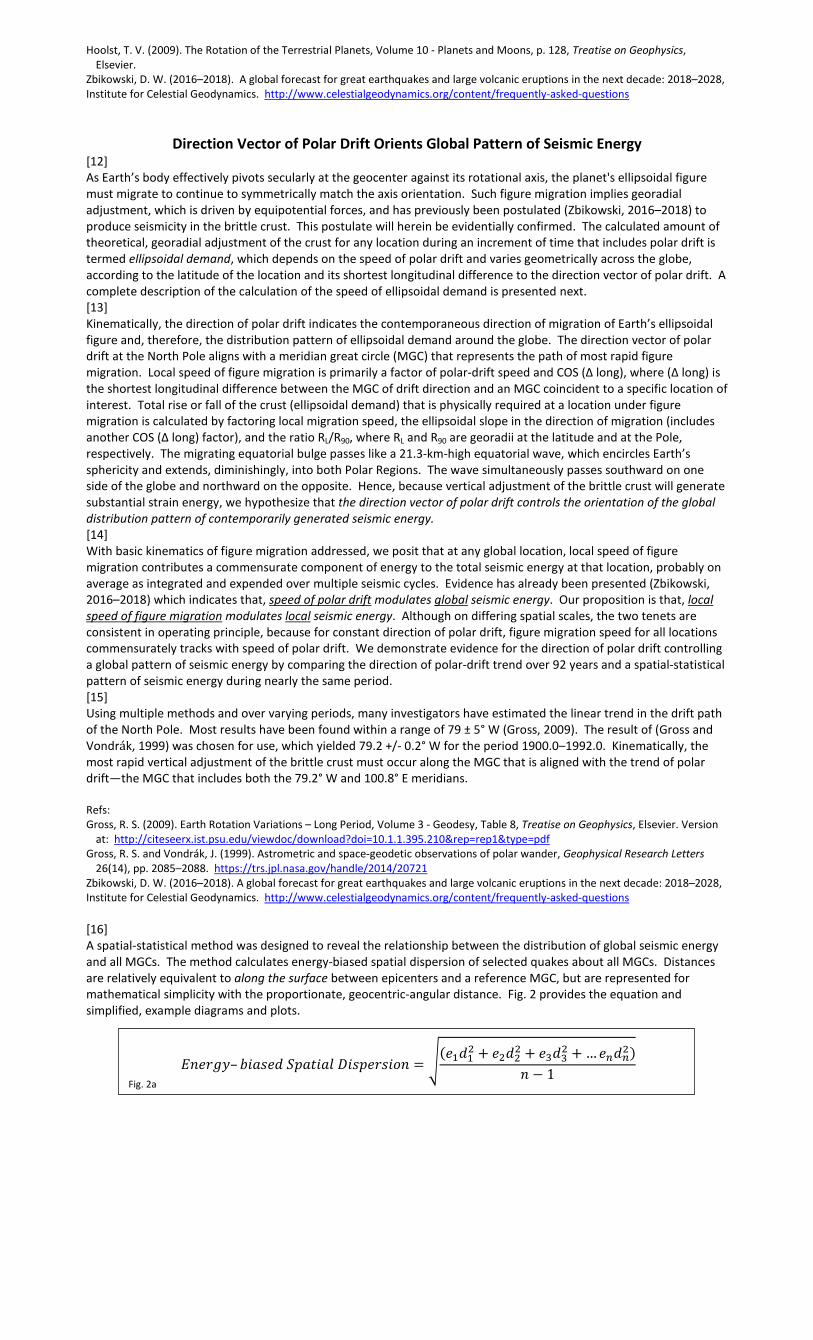
Direction Vector of Polar Drift Orients Global Pattern of Seismic Energy [12] As Earth’s body effectively pivots secularly at the geocenter against its rotational axis, the planet's ellipsoidal figure must migrate to continue to symmetrically match the axis orientation. Such figure migration implies georadial adjustment, which is driven by equipotential forces, and has previously been postulated (Zbikowski, 2016–2018) to produce seismicity in the brittle crust. This postulate will herein be evidentially confirmed. The calculated amount of theoretical, georadial adjustment of the crust for any location during an increment of time that includes polar drift is termed ellipsoidal demand, which depends on the speed of polar drift and varies geometrically across the globe, according to the latitude of the location and its shortest longitudinal difference to the direction vector of polar drift. A complete description of the calculation of the speed of ellipsoidal demand is presented next. [13] Kinematically, the direction of polar drift indicates the contemporaneous direction of migration of Earth’s ellipsoidal figure and, therefore, the distribution pattern of ellipsoidal demand around the globe. The direction vector of polar drift at the North Pole aligns with a meridian great circle (MGC) that represents the path of most rapid figure migration. Local speed of figure migration is primarily a factor of polar-drift speed and COS (∆ long), where (∆ long) is the shortest longitudinal difference between the MGC of drift direction and an MGC coincident to a specific location of interest. Total rise or fall of the crust (ellipsoidal demand) that is physically required at a location under figure migration is calculated by factoring local migration speed, the ellipsoidal slope in the direction of migration (includes another COS (∆ long) factor), and the ratio RL/R90, where RL and R90 are georadii at the latitude and at the Pole, respectively. The migrating equatorial bulge passes like a 21.3-km-high equatorial wave, which encircles Earth’s sphericity and extends, diminishingly, into both Polar Regions. The wave simultaneously passes southward on one side of the globe and northward on the opposite. Hence, because vertical adjustment of the brittle crust will generate substantial strain energy, we hypothesize that the direction vector of polar drift controls the orientation of the global distribution pattern of contemporarily generated seismic energy. [14] With basic kinematics of figure migration addressed, we posit that at any global location, local speed of figure migration contributes a commensurate component of energy to the total seismic energy at that location, probably on average as integrated and expended over multiple seismic cycles. Evidence has already been presented (Zbikowski, 2016–2018) which indicates that, speed of polar drift modulates global seismic energy. Our proposition is that, local speed of figure migration modulates local seismic energy. Although on differing spatial scales, the two tenets are consistent in operating principle, because for constant direction of polar drift, figure migration speed for all locations commensurately tracks with speed of polar drift. We demonstrate evidence for the direction of polar drift controlling a global pattern of seismic energy by comparing the direction of polar-drift trend over 92 years and a spatial-statistical pattern of seismic energy during nearly the same period. [15] Using multiple methods and over varying periods, many investigators have estimated the linear trend in the drift path of the North Pole. Most results have been found within a range of 79 ± 5° W (Gross, 2009). The result of (Gross and Vondrák, 1999) was chosen for use, which yielded 79.2 +/- 0.2° W for the period 1900.0–1992.0. Kinematically, the most rapid vertical adjustment of the brittle crust must occur along the MGC that is aligned with the trend of polar drift—the MGC that includes both the 79.2° W and 100.8° E meridians. Refs: Gross, R. S. (2009). Earth Rotation Variations – Long Period, Volume 3 - Geodesy, Table 8, Treatise on Geophysics, Elsevier. Version

at: http://citeseerx.ist.psu.edu/viewdoc/download?doi=10.1.1.395.210&rep=rep1&type=pdf Gross, R. S. and Vondrák, J. (1999). Astrometric and space-geodetic observations of polar wander, Geophysical Research Letters

26(14), pp. 2085–2088. https://trs.jpl.nasa.gov/handle/2014/20721 Zbikowski, D. W. (2016–2018). A global forecast for great earthquakes and large volcanic eruptions in the next decade: 2018–2028, Institute for Celestial Geodynamics. http://www.celestialgeodynamics.org/content/frequently-asked-questions [16] A spatial-statistical method was designed to reveal the relationship between the distribution of global seismic energy and all MGCs. The method calculates energy-biased spatial dispersion of selected quakes about all MGCs. Distances are relatively equivalent to along the surface between epicenters and a reference MGC, but are represented for mathematical simplicity with the proportionate, geocentric-angular distance. Fig. 2 provides the equation and simplified, example diagrams and plots.

𝐸𝐸𝐸𝐸𝐸𝐸𝐸𝐸𝐸𝐸𝐸𝐸– 𝑏𝑏𝑏𝑏𝑏𝑏𝑏𝑏𝐸𝐸𝑏𝑏 𝑆𝑆𝑆𝑆𝑏𝑏𝑆𝑆𝑏𝑏𝑏𝑏𝑆𝑆 𝐷𝐷𝑏𝑏𝑏𝑏𝑆𝑆𝐸𝐸𝐸𝐸𝑏𝑏𝑏𝑏𝐷𝐷𝐸𝐸 = �(𝐸𝐸1𝑏𝑏12 + 𝐸𝐸2𝑏𝑏22 + 𝐸𝐸3𝑏𝑏32 + … 𝐸𝐸𝑛𝑛𝑏𝑏𝑛𝑛2)𝐸𝐸 − 1

Fig. 2a

[17] FIGURE 2 Fig. 2a provides the spatial-dispersion equation where e factors are seismic energies of quakes and d components are geocentric-angular distances between epicenters and a reference MGC. Fig. 2c shows the diagram of Fig. 2b after exchanging a typical quake with a much larger quake on the eastern side of the 130° E MGC. The Fig. 2c plot shows the resulting shift to the right of the dispersion trace’s low point and narrower ‘valley’ profile.

[18] FIGURE 3

Traces in Fig. 3 display dispersion of global seismic energy about all MGCs for quakes grouped by Ms category with all quakes of Ms ≥ 6.5 and focal depth ≤ 150 km as recorded from 1905–2005. The term ‘w/ E Bias’ in the Y-axis label means that each distance2 component was factored by the seismic energy of the quake—similar graphs were explored without energy bias. Two U.S.G.S. quake catalogs were searched, Significant Worldwide Earthquakes 2150 BC–1994 AD, and USGS NEIC (PDE) 1973–Present (Quake Data, 1905–2005). Ms was utilized as the measure of magnitude in the first database. Hence, to express quake energy with a consistent measure, allowing uncomplicated calculation of spatial dispersion, use of Ms was continued. Fig. 3 groups quakes by Ms in an inclusively bracketed manner—each quake category includes all larger quakes. (The resulting effects of exclusive bracketing are shown in Fig. 4 for comparison.) For each (eastern referenced) MGC from 0–180° in 0.5° increments, dispersion is calculated using (smallest geocentric angle)2 deviations, which are proportionate to (shortest surface distance)2 deviations of epicenters from the nearest meridian of the reference MGC.

Data Assumptions

[19] Quakes of Ms < 6.5 generally represent less than 10% of global seismic energy and so were considered unnecessary to reveal a dominant global pattern and this assumption proved correct. The ‘focal-depth ≤ 150 km’ criterion was intended to include seismicity from crustal faults and interplate dynamics, but to avoid seismicity from deep sources associated with well-descended slabs, chemical phase transitions, or compositional processes, all of which are less related to crustal strain and, presumably, plate motions. Although seismic behavior of the lithosphere was probably generally consistent during 1905–2005, the combination of the two U.S.G.S. databases shows a substantial increase in the number of 6.5 ≤ Ms < 7.5 quakes, starting in 1973 and predominantly from the NEIC record. Relatedly, because the sensitivity and distribution of seismographs has varied so greatly during this period, valid questions may be raised concerning the accuracy of any quake databases that cover most of that time.

Interpretation [20] In Fig. 3, low points on dispersion traces identify eastern meridians of MGCs that most closely fit the global distribution of seismic energy for each category of quake magnitude. Dispersion traces of the inclusively bracketed quake groupings show that, statistically, the greater a quake’s energy, the more closely its epicenter MGC matches the MGC of the polar-drift trend at 100.8° E. This observation supports a previously introduced hypothesis that, the larger the quake, the more it requires all stress-loading components of triggering impetus to be near optimal configuration—

Fig. 2c Fig. 2b

EM1

EM2

EM3

EM4

EӨ

tectonic loading, ellipsoidal demand, and earth tides (Zbikowski, 2014–2017). Quakes of lesser energy pull the points of lowest dispersion to the right on the graph. Hence, it appears that there could be more than one action mode (e.g. ellipsoidal demand, plate interactions) determining the global distribution of seismic energy. Because the largest great quakes supply the majority of global seismic energy, migration of Earth’s figure via ellipsoidal demand driven by equipotential adjustments appears to cause (generate and trigger) more global seismic energy than convection-related processes alone. Ref: Quake Data, (1905–2005). Data source was the USGS Earthquake Hazards Program website. Under Global Search Area two

databases were searched: (1) Significant Worldwide Earthquakes 2150 BC –1994 AD, and (2) USGS NEIC (PDE) 1973 –Present. Quakes were selected with a magnitude of Ms ≥ 6.5 and focal depth ≤ 150 km that occurred from 01 Jan 1905 to 03 Oct 2005 (present). Ms was utilized as the measure of magnitude in the first database. Hence, to express quake energy with a consistent measure, allowing uncomplicated calculation of spatial dispersion, use of Ms was continued.

Zbikowski, D. W. (2014–2017). Apparent Triggering of Large Earthquakes in Los Angeles and San Francisco Regions Related to Time Derivatives of Ellipsoidal Demand, Kinematically Derived: Qualitative Interpretations for 1890–2014.1, Institute for Celestial Geodynamics. http://www.celestialgeodynamics.org/content/los-angeles-san-francisco

[21] FIGURE 4

Traces in Fig. 4 display dispersion of global seismic energy about all MGCs for the same 1,818 quakes, now grouped by Ms in an exclusively bracketed manner—each trace represents only quakes of magnitudes within its narrow, double-bounded category. See description of Fig. 3 for remaining details.

Interpretation

[22] Exclusively bracketed sorting enables individual categories to express most directly their specific spatial inclinations, hinting to source regions or energizing modes of quakes, without the overwhelming energetic bias of all larger quakes that inclusive sorting includes. The use of exclusive sorting shows more clearly that, statistically, the greatest quakes are located nearer to 102° E / 78° W (e.g. Sumatra; or Ecuador, Peru, and Chile—the American Pacific Rim) and, therefore, appear to utilize the greatest component of ellipsoidal demand to trigger and partially load (not completely load, because forces on plates that derive from convection processes are also contributing). Analogously, the smaller the quake, the more its location tends closer to 132° E / 48° W (e.g. Japan, New Guinea—the Asian Pacific Rim), with the category of smallest quakes, 6.5 ≤ Ms ≤ 7.0, coinciding with this region. This MGC, along the Asian Pacific Rim, represents a global region of particularly numerous quakes. Because of the many quakes in this region of remarkably active plate collision and especially subduction, this magnitude category expresses an energy bias that results from plate interactions. Further, worldwide, this trace is very flat, meaning a rather even global distribution of such sized quakes that result from plate interactions. To summarize, Fig. 4 (1) identifies an MGC that uniquely best-fits greatest energy quakes, closely matches the average trend of polar drift, and kinematically represents the central maximum in the hypothesized bulge-migration mode of seismic energy generation, (2) indicates a different MGC that best-fits lower energy quakes, matches a very seismic global region, and presents a worldwide uniform bias that may derive largely from the plate interactions mode of seismic energy generation, and (3) displays systematic, global regularity of both modes by exhibiting a pattern of distribution traces that blends consistently across magnitude categories. Hence, Fig. 4 seems to demonstrate broadly effective resolution to this spatial-statistical representation. Refs: Gross, R. S. and Vondrák, J. (1999). Astrometric and space-geodetic observations of polar wander, Geophysical Research Letters

26(14), pp. 2085–2088. https://trs.jpl.nasa.gov/handle/2014/20721 Gross, R. S. (2009). Earth Rotation Variations – Long Period, Volume 3 – Geodesy, Table 8, Treatise on Geophysics, Elsevier. Version

at: http://citeseerx.ist.psu.edu/viewdoc/download?doi=10.1.1.395.210&rep=rep1&type=pdf Zbikowski, D. W. (2014–2017). Apparent Triggering of Large Earthquakes in Los Angeles and San Francisco Regions Related to Time

Derivatives of Ellipsoidal Demand, Kinematically Derived: Qualitative Interpretations for 1890–2014.1, Institute for Celestial Geodynamics. http://www.celestialgeodynamics.org/content/los-angeles-san-francisco

Zbikowski, D. W. (2016–2018). A global forecast for great earthquakes and large volcanic eruptions in the next decade: 2018–2028, Institute for Celestial Geodynamics. http://www.celestialgeodynamics.org/content/frequently-asked-questions

EM5

EM6

EMӨ

EM7 EM8

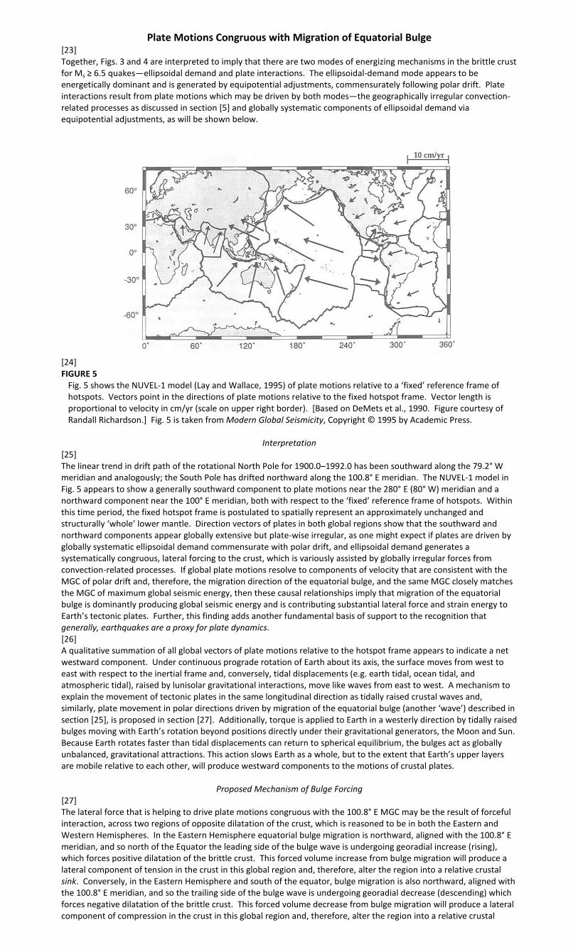
Plate Motions Congruous with Migration of Equatorial Bulge [23] Together, Figs. 3 and 4 are interpreted to imply that there are two modes of energizing mechanisms in the brittle crust for Ms ≥ 6.5 quakes—ellipsoidal demand and plate interactions. The ellipsoidal-demand mode appears to be energetically dominant and is generated by equipotential adjustments, commensurately following polar drift. Plate interactions result from plate motions which may be driven by both modes—the geographically irregular convection-related processes as discussed in section [5] and globally systematic components of ellipsoidal demand via equipotential adjustments, as will be shown below.

[24] FIGURE 5

Fig. 5 shows the NUVEL-1 model (Lay and Wallace, 1995) of plate motions relative to a ‘fixed’ reference frame of hotspots. Vectors point in the directions of plate motions relative to the fixed hotspot frame. Vector length is proportional to velocity in cm/yr (scale on upper right border). [Based on DeMets et al., 1990. Figure courtesy of Randall Richardson.] Fig. 5 is taken from Modern Global Seismicity, Copyright © 1995 by Academic Press.

Interpretation

[25] The linear trend in drift path of the rotational North Pole for 1900.0–1992.0 has been southward along the 79.2° W meridian and analogously; the South Pole has drifted northward along the 100.8° E meridian. The NUVEL-1 model in Fig. 5 appears to show a generally southward component to plate motions near the 280° E (80° W) meridian and a northward component near the 100° E meridian, both with respect to the ‘fixed’ reference frame of hotspots. Within this time period, the fixed hotspot frame is postulated to spatially represent an approximately unchanged and structurally ‘whole’ lower mantle. Direction vectors of plates in both global regions show that the southward and northward components appear globally extensive but plate-wise irregular, as one might expect if plates are driven by globally systematic ellipsoidal demand commensurate with polar drift, and ellipsoidal demand generates a systematically congruous, lateral forcing to the crust, which is variously assisted by globally irregular forces from convection-related processes. If global plate motions resolve to components of velocity that are consistent with the MGC of polar drift and, therefore, the migration direction of the equatorial bulge, and the same MGC closely matches the MGC of maximum global seismic energy, then these causal relationships imply that migration of the equatorial bulge is dominantly producing global seismic energy and is contributing substantial lateral force and strain energy to Earth’s tectonic plates. Further, this finding adds another fundamental basis of support to the recognition that generally, earthquakes are a proxy for plate dynamics. [26] A qualitative summation of all global vectors of plate motions relative to the hotspot frame appears to indicate a net westward component. Under continuous prograde rotation of Earth about its axis, the surface moves from west to east with respect to the inertial frame and, conversely, tidal displacements (e.g. earth tidal, ocean tidal, and atmospheric tidal), raised by lunisolar gravitational interactions, move like waves from east to west. A mechanism to explain the movement of tectonic plates in the same longitudinal direction as tidally raised crustal waves and, similarly, plate movement in polar directions driven by migration of the equatorial bulge (another ‘wave’) described in section [25], is proposed in section [27]. Additionally, torque is applied to Earth in a westerly direction by tidally raised bulges moving with Earth’s rotation beyond positions directly under their gravitational generators, the Moon and Sun. Because Earth rotates faster than tidal displacements can return to spherical equilibrium, the bulges act as globally unbalanced, gravitational attractions. This action slows Earth as a whole, but to the extent that Earth’s upper layers are mobile relative to each other, will produce westward components to the motions of crustal plates.

Proposed Mechanism of Bulge Forcing [27] The lateral force that is helping to drive plate motions congruous with the 100.8° E MGC may be the result of forceful interaction, across two regions of opposite dilatation of the crust, which is reasoned to be in both the Eastern and Western Hemispheres. In the Eastern Hemisphere equatorial bulge migration is northward, aligned with the 100.8° E meridian, and so north of the Equator the leading side of the bulge wave is undergoing georadial increase (rising), which forces positive dilatation of the brittle crust. This forced volume increase from bulge migration will produce a lateral component of tension in the crust in this global region and, therefore, alter the region into a relative crustal sink. Conversely, in the Eastern Hemisphere and south of the equator, bulge migration is also northward, aligned with the 100.8° E meridian, and so the trailing side of the bulge wave is undergoing georadial decrease (descending) which forces negative dilatation of the brittle crust. This forced volume decrease from bulge migration will produce a lateral component of compression in the crust in this global region and, therefore, alter the region into a relative crustal

source. The crust of the two global regions north and south of the Equator will be pulled toward the sink, which, because of the surface slope along the Earth ellipsoid, has a maximum lateral component of tension at about 45° N, 100.8° E; and pushed from the source, which has a maximum lateral component of compression at about 45° S, 100.8° E. This S-to-N forcing will drive a lateral component of crustal motion relative to the hotspot frame, which will manifest as congruous, S-to-N components to regional plate motions. Similarly, in the Western Hemisphere, opposite forcing N-to-S will drive a lateral component of crustal motion relative to the hotspot frame and aligned with the 280.8° E (79.2° W) meridian, which will manifest as regional plate motions with congruous, N-to-S components aligned with the 79.2° W meridian. This globally symmetrical, bulge-forcing effect applied to the motions of plates with respect to the hotspot frame is subtle, but clearly recognizable on the NUVEL-1 model. [28] Spatial-statistical analysis of global seismic energy, using energy-biased dispersions about MGCs, clearly shows promise as a powerful new tool for investigating the relationships between seismology and geodynamics. Based on this success, it seems possible that by extending the method into a latitudinal extent and exploring further, additional new patterns or relationships may be revealed. Therefore, the peridian framework is introduced next to allow investigating such relationships more thoroughly. Refs: DeMets, C., Gordon, R. G., Argus, D.F., and Stein, S. (1990). Current plate motions, Geophys. J. Int., 101, pp. 425–478.

https://www.researchgate.net/publication/227822173_Current_Plate_Motions http://onlinelibrary.wiley.com/doi/10.1111/j.1365-246X.1990.tb06579.x/abstract

Lay, T. and Wallace, T.C. (1995). Modern Global Seismicity, p. 438, Figure 11.4, Academic Press, CA. Figure based on DeMets et al., 1990. Permission courtesy of Randall Richardson.

Dispersion of Global Seismic Energy with respect to the Peridian Framework [29] Having polar orientations, MGCs are useful to statistically analyze longitudinally oriented spatial patterns of seismic energy, worldwide. To similarly analyze related distribution patterns in a latitudinal orientation, with respect to the longitudinal dimension, peridian great circles (PGCs) are introduced. For every MGC, a global set of PGCs exists and the combination of both aspects creates an analytical space within which distribution patterns of seismic energy may reveal hints to sources or modes of subtle energizing and/or triggering effects for quakes. Fig. 6 illustrates the peridian framework that is proposed.

[30] FIGURE 6

Fig. 6 illustrates a global set of PGCs for a single MGC. PGCs are oriented perpendicular to MGCs and are designed to present a means of continuing related seismic-energy dispersion analysis into a latitudinal dimension. For each MGC from 0°–180° E in 1.0° increments, we will statistically analyze a set of PGCs oriented as shown from 0°–180° N, in 0.2° increments. Similar to MGC analysis, the PGC best-fitting global seismic energy will have the lowest energy dispersion (LEDPGC) for that MGC.

[31] Dispersions of seismic energy will be calculated for all PGCs in complete sets, for all MGCs in 1.0° increments around the globe. In Figs. 7 and 8, sets of energy dispersions of PGCs (EDPGCs) for two specific MGCs are examined and general attributes noted. These two MGCs have been selected by rationale that will be explained later. Also, several runs of random epicenters, with limits of latitude made to duplicate the record of historical epicenters, were performed as test controls and a typical result using random data is shown in Fig. 9. After comparing attributes of results from actual data and random-data runs, some speculation regarding physical mechanisms is discussed.

[32] FIGURE 7

Fig. 7 shows energy dispersions of PGCs (EDPGCs, solid traces) calculated for the MGC of 71° E, using Ms ≥ 7.6 quakes with focal depths ≤ 150 km from the same two U.S.G.S. databases (Quake Data, 1905-2005). PGCs in 0.2° increments were analyzed to increase resolution in the equatorial to mid-latitudes, which host most of the seismic energy. As required by limited computational capacity, a reduction in data, from 1,818 to 407 quakes, was accomplished by selecting only Ms ≥ 7.6 quakes. The term ‘w/ E Bias’ in the Y-axis label means that each distance2 component was factored by the seismic energy of the quake—similar graphs were explored without energy bias. Dotted traces paired to the solid traces are sinusoidal constructs that are designed to be of the same period, amplitude, and phase, as their matched dispersion traces.

Interpretation

[33] The choice of the reference MGC of 71° E in Fig. 7 will be explained in sections [40–45]. Solid lines are dispersion traces for three inclusive categories of magnitude. Dispersion traces match their sinusoidal counterparts closely. Fig. 7 shows that for the MGC of 71° E, the PGC of lowest energy dispersion (LEDPGC) for all 407 quakes is 25.6° N. For the three inclusive categories, which characterize peridian seismic energy for this MGC, little variation (0.4°) exists in LEDPGCs. Therefore, quakes alternatively grouped exclusively by magnitude would show only minor variation in LEDPGC from the inclusively grouped examples shown. However, as category ranges include fewer small quakes, amplitudes of the waveform envelopes increase. This observation in the latitudinal dimension of PGCs seems consistent with the similar observation in the longitudinal dimension of MGCs that smaller quakes tend to be more uniformly distributed, globally. Two contributing factors vary with respect to the latitudinal dimension and may help to determine the distribution of seismic energy in relation to peridians: (1) globally, latitudinal variations in ellipsoidal geometry affect local ellipsoidal demand and, (2) Earth’s obliquity (angle between its equatorial plane and orbital plane) of 23.44° controls the seasonal latitude of maximum vertical displacement from lunisolar earth tides and also factors into the polar torque that Earth receives from the Moon, Sun, and celestial neighbors, which, as developed herein, drives polar drift and, as will be developed in Part 2, appears to determine the mathematical trajectory of polar wander. Polar drift and global geometry both factor into the energizing (crustal loading) and triggering impetus of quakes (Zbikowski, 2014–2017).

[34] FIGURE 8

Fig. 8 shows EDPGCs (solid traces) calculated for the MGC of 131° E, using M ≥ 7.6 quakes with focal depths ≤ 150 km from the same two U.S.G.S. databases (Quake Data, 1905-2005). The remainder of this description is identical to content in the description of Fig. 7.

0 10 20 30 40 50 60 70 80 90 100 110 120 130 140 150 160 170 1800

20406080

100120140160180200220240260280300320340360380400

Dispersion of Quake Energy about PGCs

DEGREES NORTH LATITUDE

Disp

ersio

n (d

eg-jo

ule/

fact

or) w

/ E B

ias

DispE1

DispE2

DispEΘ

SineFitE1

SineFitE2

SineFitEΘ

Peridian

MGC 71° E Peridian of Lowest Dispersion E1: Ms ≥ 8.5 (31 ea.) = 25.5°N E2: Ms ≥ 8.2 (92 ea.) = 25.9°N EΘ: Ms ≥ 7.6 (407 ea.) = 25.6°N

MGC 131° E Peridian of Lowest Dispersion E1: Ms ≥ 8.5 (31 ea.) = 17.2°N E2: Ms ≥ 8.2 (92 ea.) = 17.7°N EΘ: Ms ≥ 7.6 (407 ea.) = 17.4°N

E1

E2

EӨ

E1

E2

EӨ

Interpretation [35] The choice of the reference MGC of 131° E in Fig. 8 will be explained in sections [40–45]. Solid lines are dispersion traces for three inclusive categories of magnitude. Dispersion traces match their sinusoidal counterparts closely. Fig. 8 shows that for the MGC of 131° E, the LEDPGC for all 407 quakes is 17.4° N. For the three inclusive magnitude categories, which characterize peridian seismic energy for this MGC, little variation (0.5°) exists in LEDPGCs and so an exclusive treatment for comparison is unnecessary. The remainder of this interpretation is identical to content in the interpretation of Fig. 7. [36] To investigate more thoroughly whether dispersions of global seismic energy in the PGC dimension yield patterns that are physically meaningful, several dispersion trials using matched sets of ‘randomized’ data were run. Fig. 9 illustrates results that are typical of the random-data trials.

[37] FIGURE 9

Fig. 9 shows EDPGCs (solid traces) calculated for a generic MGC. The matched set of ‘randomized’ data (407 events) are modified data—randomly containing the same magnitudes as the actual data and modified with random locations within imposed bounding latitudes that matched the historically determined range (62.8° S to 70.4° N). This procedure was followed because using the actual magnitudes sited at random locations avoids any geographic bias, and the bounded latitudinal range avoids a distortion of density of seismic energy from a more uniform global distribution that is never experienced in reality.

Interpretation

[38] Fig. 9 illustrates characteristics that are typical of several randomized trials:

1. Amplitudes of waveform envelopes of dispersion traces for a magnitude category are much reduced (typically half or less) in random-data trials vs. runs using actual seismicity. Reduced waveform envelopes indicate that seismic energy in random trials is more evenly distributed within the imposed bounds of latitude than in runs using actual quake data. This result may derive, in part, from the lack of modelled tectonic plates that tend to focus quakes along their margins.

2. Agreement to sinusoidal counterparts are not as good in random-data trials, as compared to actual runs for the selected MGCs (71° E and 131° E), especially for larger magnitude categories. Because the selected two runs using actual seismicity show better sinusoidal agreement, and because vectors of gravitational attraction between Earth and a remote mass can be approximated to converge to a remote focus, if such interaction is sufficient to directly increase seismic energy, a global pattern of relative dispersion of seismic energy may present itself geometrically. A sinusoidal character might be produced from such an interaction, if forces normal to the crustal surface trigger quakes commensurate with force magnitude, because gravitational vectors to remote masses should resolve sinusoidally (approximately [4]) along normals to Earth’s surface. Even a minor influence might show up, statistically, in this analysis, if the effect overprints an otherwise generally uniform distribution of seismic energy in the peridian dimension. Hence, we hypothesize that when a dispersion trace in the PGC dimension is most sinusoidal, substantial seismic causation may be inferred as being due to the gravity of Solar System bodies. The issue clearly justifies further investigation.

3. Peaks of dispersion traces in random-data trials are not restricted to polar latitudes, as they are in runs using actual seismicity. The scatter of peaks may result simply because LEDPGCs are not restricted to regions near the Northern (or Southern) Tropic, as appears to be common in runs using actual quakes for the selected meridians. This difference begs the question, “What mechanism(s) favor such positioning of quakes, as near (25.6° + 17.4°)/2 = 21.5° N peridian. We postulate that three geophysical factors may be variously involved: (a) For a given drift speed and global longitude, maximum ellipsoidal demand occurs at 44.9° N and 44.9° S latitudes, because of the compound effect of varying surface slope (ellipsoidal figure) and georadius. (b) Georadial vectors of gravitational forces to the Moon, Sun, and other neighboring planets of the Solar System, lie on or within a few degrees of Earth’s orbital plane (ecliptic). Earth’s obliquity (23.44°) is the angle between the equatorial plane and the ecliptic. Dominant gravitational forces are applied from within (or very near) the ecliptic, which always intersects the surface of the Earth at latitudes between ± 23.44°. Hence, for each meridian, the georadial vector that is aligned with the plane of ecliptic gravity cycles in latitude from 0° to 23.44° S to 0° to 23.44° N to 0° on a daily basis. Therefore, earth-tidal effects will be maximized in that range of latitudes on Earth, over orbital periods (i.e. Sun, Moon) or synodic periods (e.g. Venus, Mars, Jupiter). (c) Because of rotational effects, maximum heat transfer

0 10 20 30 40 50 60 70 80 90 100 110 120 130 140 150 160 170 1800

20406080

100120140160180200220240260280300320340360380400

Dispersion of Quake Energy about PGCs

DEGREES NORTH LATITUDE

Disp

ersio

n (d

eg-jo

ule/

fact

or) w

/ E B

ias

DispE1

DispE2

DispEΘ

SineFitE1

SineFitE2

SineFitEΘ

Peridian

MGC XX° E Peridian of Lowest Dispersion E1: Ms ≥ 8.5 (31 ea.) = 85.5°N E2: Ms ≥ 8.2 (92 ea.) = 85.7°N EΘ: Ms ≥ 7.6 (407 ea.) = 85.6°N

E1

E2

EӨ

from Earth’s Outer Core appears robustly in models to flow within a narrow equatorial zone (Glatzmaier and Roberts, 1995)(Glatzmaier, 1999).

[39] Therefore, for actual seismicity in the peridian dimension there are three identified physical mechanisms that both accentuate variation in the distribution of seismic energy and mechanistically partition the globe relative to latitude. The combination of these mechanisms, applied in presently unknown proportions, is speculated to be capable of supporting LEDPGCs near the 21.5° N peridian. Note: 4. The Moon is too close to Earth for the sinusoidal character to be more than approximate for the full globe. However, this

sinusoidal approximation is especially close in the range of latitudes where most seismic energy is released (e.g. ± 45° lat.). Refs: Glatzmaier, G. A., and P. H. Roberts (1995). A three-dimensional convective dynamo solution with rotating and finitely conducting

inner core and mantle, Phys. Earth Planet. Inter., 91, pp. 63–75. Glatzmaier, G. A. (1999). In private email correspondence with Douglas Zbikowski, Glatzmaier stated that his convection models

had robustly shown an equatorial zone of highest heat transfer.

Attributes of EDPGCs for MGCs around the Globe [40] In Fig. 10, two attributes of EDPGCs are shown for 407 quakes of M ≥ 7.6, for MGCs around the globe. The first (ΘAmp, blue trace) shows amplitudes of waveform envelopes of EDPGCs, which plot a line showing peak amplitude of envelope at an MGC (97° E) that approximates the trend of polar drift (100.8°E). The second (ΘDSin, red trace) displays integrated differences between waveforms of EDPGCs and constructed sinusoidal counterparts. The two attributes are paired in ratio (ΘAmp/ ΘDSin), sequentially, and the results (FitEΘ, brown trace) are reasoned to indicate a measure of gravitational effect of Solar System neighbors within or near the ecliptic.

[41] FIGURE 10

Fig. 10 illustrates how two attributes of traces of EDPGCs vary—amplitude of waveform envelope (ΘAmp, blue trace) and integrated differences between waveforms and constructed sinusoidal counterparts that are made to be of the same amplitude, wavelength, and phase (ΘDSin, red trace)—as well as the ratio (ΘAmp/ ΘDSin) between them (FitEΘ, brown trace). Attributes were calculated using 407 quakes of M ≥ 7.6 with focal depths ≤ 150 km, for MGCs around the globe. The ‘Meridian’ label on the X axis denotes ‘°E longitude’ per convention.

Interpretation

[42] ΘAmp The blue trace is comprised of amplitudes of waveform envelopes for EDPGCs, for all MGCs around the globe. The trace peak at 97° E MGC approximates the MGC of the polar-drift trend at 100.8° E, with both determinations using data from nearly matching periods (i.e. quakes: 1905–2005, polar drift: 1900–1992). The MGC of greatest amplitude of envelope is reasoned to occur near the MGC of greatest migration speed (and greatest seismic energy ‘density’), simply because seismic energy variations in the meridian and peridian dimensions are not mutually exclusive and so the peridian dimension is also likely to show its global-maximum range there. Hence, the approximate matching of the MGC of greatest amplitude of envelope with the MGC of polar-drift trend adds further evidence supporting the bulge-forcing hypothesis, this time from within the peridian dimension. [43] ΘDSin The red trace is comprised of the integrated differences between EDPGC waveforms and constructed sinusoidal counterparts that are made to be of the same amplitude, wavelength, and phase for all 407 quakes with focal depths ≤ 150 km, for MGCs around the globe. The ΘDSin trace peaks sharply at 96° E. As was noted in sections [33] and [35], for categories of higher magnitude quakes, EDPGC traces show greater amplitude of envelope (blue line height) and greater deviation from their sinusoidal counterparts (red trace height). The red trace, here calculated using 407 quakes of M ≥ 7.6, seems to follow this amplitude/variance proportional tracking for the -/+ 30° span around its peak amplitude at 96° E MGC. Again, as discussed in section [38(point 2)], the agreement of the EDPGC trace to its sinusoidal counterpart is hypothesized to be an indicator of a physical mechanism that involves vectors of gravitational attraction at Earth’s surface to neighboring celestial bodies (e.g. Moon and Sun) within or near the ecliptic. [44] FitEΘ The brown trace is comprised of ratios of the above two attributes formed by taking (ΘAmp/ ΘDSin). Two peaks are on this trace, at MGCs of 71° E and 131° E, each of which is 30° on an alternate side of the MGC of polar-drift trend. The traces of EDPGCs for these two MGCs were shown above in Figs. 7 and 8. Because these peaks are

0 10 20 30 40 50 60 70 80 90 100 110 120 130 140 150 160 170 1800

1

2

3

4

5

6

7

8

9

10

0

8

16

24

32

40

48

56

64

72

80

EDispEΘDSinEDispEΘAmp

EBestFitEΘ

Meridian

ӨAmp

ӨDSin

FitEӨ

positioned precisely symmetrical to the MGC of polar drift, the symmetry may indicate reliance of these attributes on the speed of bulge migration. [45] The Moon has approximately twice the earth-tide generating effect of the Sun on Earth and so, if earth-tidal displacements assist in triggering many quakes, it reasonably follows that the LEDPGC for each MGC should reside somewhat near the orbital plane of the Moon (see Fig. 11). The mean orbital plane of the Moon is inclined 5.14° to the ecliptic. Because of Earth’s obliquity, the Sun’s declination ranges from 23.44° S in winter to 23.44° N in summer. Due to the lunar, revolution-of-node cycle, the Moon varies in declination between (23.44° + 5.14°) = 28.58° N or S, and (23.44° - 5.14°) = 18.3° N or S for a complete lunar-nodal cycle of 18.61 years. These outer limits in declination are met when Earth’s rotational axis is orthogonal to a line joining the lunar nodes (twice per 18.61 years). During a sidereal month, the lunar declination cycles between + and – values. Using the peridian framework convention, only PGCs in the Northern Hemisphere will be referenced, so the outer limits of the lunar orbital plane will reside at 28.58° N and 18.3° N. In Fig. 10, the first peak of FitEΘ (brown trace), at 71° E, has an LEDPGC at 25.6° N (see Fig. 7), which is near midpoint between maximum declination of both the ecliptic and the Moon (23.44° + 5.14°/2) = 26.01° N (see Fig. 11). The second peak of FitEΘ, at 131° E, has an LEDPGC at 17.4° N (see Fig. 8), which is near the lunar limit of 18.3° N. Hence, because earth-tidal displacements are maximized for a given separation distance when a celestial body is at zenith, these results seem to indicate that earth-tidal displacements by the Moon and Sun are statistically significant in assisting quake triggering on Earth. Therefore, these two attributes of EDPGCs for MGCs around the globe, when utilized in ratio to reveal peak values, may indicate correlation between latitudinal patterns of epicenters of large quakes and orbital configurations of Earth, Moon, and the Sun. [46] Additionally, superposition of substantially strong gravitational fields exchanged between Earth and the Moon and Sun during syzygy (i.e. solar eclipses, lunar eclipses, and to a lesser degree New Moon and Full Moon) provokes non-linear responses due to (1) non-linear potentials across intervening distances and (2) non-linearity in the material strain response of the non-rigid Earth. Gravitational potentials and material responses (e.g. surface displacement) are maximized during such alignments and extrema of gravitational jerk and jounce just before and just after syzygy may act as substantial impetuses to trigger large quakes (Zbikowski, 2014–2017).

[47] FIGURE 11

Fig. 11 diagrams Earth’s orbital dance with the Moon and Sun. The cartoon shows configurations of the Earth, Moon, and Sun when the Sun is at minimum declination on the winter solstice (about Dec 21) and the Moon is at the maximum declination within the 18.61-year lunar-nodal cycle. The Moons on the left and right are separated in time by half of a synodic month. The PGC in best alignment with the vector of maximum gravitational pull of the Sun and either Moon is between the ecliptic, 23.44° N, and the lunar orbital plane (23.44° + 5.14°) = 28.58° N. After the Moon passes halfway through its revolution-of-node cycle and again on Dec 21, the PGC in best alignment will be between 23.44° N and (23.44°-5.14°) = 18.3° N.

[48] The selection procedure for MGCs of 71° E and 131° E uses physical rationale that is hypothesized to involve LEDPGCs which exhibit dominant gravitational effects from the Moon, Sun, and planetary masses. To understand the full extent of these gravitational effects on global seismic energy in the peridian dimension, Fig. 12 was created.

26° PGC

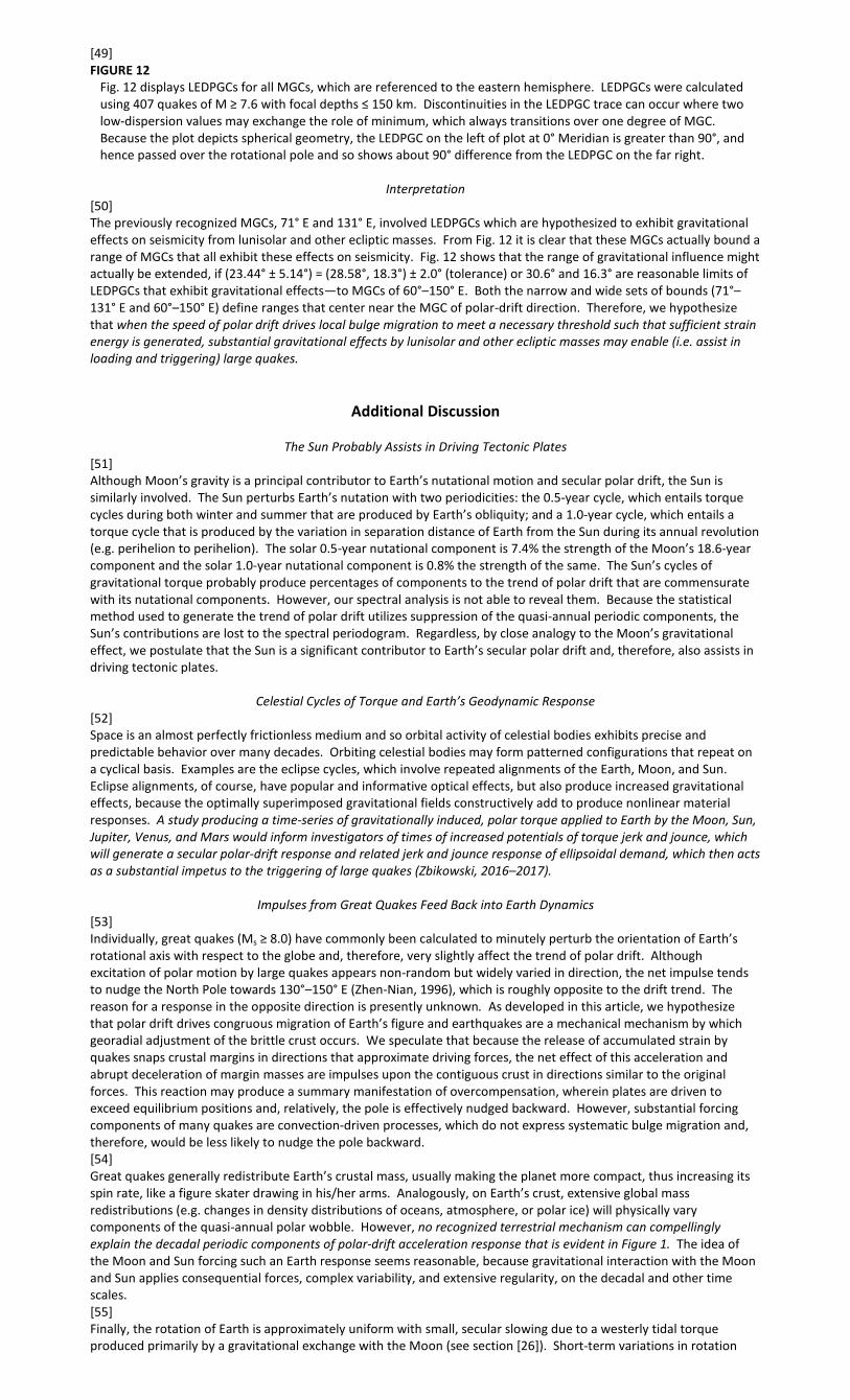
[49] FIGURE 12

Fig. 12 displays LEDPGCs for all MGCs, which are referenced to the eastern hemisphere. LEDPGCs were calculated using 407 quakes of M ≥ 7.6 with focal depths ≤ 150 km. Discontinuities in the LEDPGC trace can occur where two low-dispersion values may exchange the role of minimum, which always transitions over one degree of MGC. Because the plot depicts spherical geometry, the LEDPGC on the left of plot at 0° Meridian is greater than 90°, and hence passed over the rotational pole and so shows about 90° difference from the LEDPGC on the far right.

Interpretation

[50] The previously recognized MGCs, 71° E and 131° E, involved LEDPGCs which are hypothesized to exhibit gravitational effects on seismicity from lunisolar and other ecliptic masses. From Fig. 12 it is clear that these MGCs actually bound a range of MGCs that all exhibit these effects on seismicity. Fig. 12 shows that the range of gravitational influence might actually be extended, if (23.44° ± 5.14°) = (28.58°, 18.3°) ± 2.0° (tolerance) or 30.6° and 16.3° are reasonable limits of LEDPGCs that exhibit gravitational effects—to MGCs of 60°–150° E. Both the narrow and wide sets of bounds (71°–131° E and 60°–150° E) define ranges that center near the MGC of polar-drift direction. Therefore, we hypothesize that when the speed of polar drift drives local bulge migration to meet a necessary threshold such that sufficient strain energy is generated, substantial gravitational effects by lunisolar and other ecliptic masses may enable (i.e. assist in loading and triggering) large quakes.

Additional Discussion

The Sun Probably Assists in Driving Tectonic Plates [51] Although Moon’s gravity is a principal contributor to Earth’s nutational motion and secular polar drift, the Sun is similarly involved. The Sun perturbs Earth’s nutation with two periodicities: the 0.5-year cycle, which entails torque cycles during both winter and summer that are produced by Earth’s obliquity; and a 1.0-year cycle, which entails a torque cycle that is produced by the variation in separation distance of Earth from the Sun during its annual revolution (e.g. perihelion to perihelion). The solar 0.5-year nutational component is 7.4% the strength of the Moon’s 18.6-year component and the solar 1.0-year nutational component is 0.8% the strength of the same. The Sun’s cycles of gravitational torque probably produce percentages of components to the trend of polar drift that are commensurate with its nutational components. However, our spectral analysis is not able to reveal them. Because the statistical method used to generate the trend of polar drift utilizes suppression of the quasi-annual periodic components, the Sun’s contributions are lost to the spectral periodogram. Regardless, by close analogy to the Moon’s gravitational effect, we postulate that the Sun is a significant contributor to Earth’s secular polar drift and, therefore, also assists in driving tectonic plates.

Celestial Cycles of Torque and Earth’s Geodynamic Response [52] Space is an almost perfectly frictionless medium and so orbital activity of celestial bodies exhibits precise and predictable behavior over many decades. Orbiting celestial bodies may form patterned configurations that repeat on a cyclical basis. Examples are the eclipse cycles, which involve repeated alignments of the Earth, Moon, and Sun. Eclipse alignments, of course, have popular and informative optical effects, but also produce increased gravitational effects, because the optimally superimposed gravitational fields constructively add to produce nonlinear material responses. A study producing a time-series of gravitationally induced, polar torque applied to Earth by the Moon, Sun, Jupiter, Venus, and Mars would inform investigators of times of increased potentials of torque jerk and jounce, which will generate a secular polar-drift response and related jerk and jounce response of ellipsoidal demand, which then acts as a substantial impetus to the triggering of large quakes (Zbikowski, 2016–2017).

Impulses from Great Quakes Feed Back into Earth Dynamics [53] Individually, great quakes (Ms ≥ 8.0) have commonly been calculated to minutely perturb the orientation of Earth’s rotational axis with respect to the globe and, therefore, very slightly affect the trend of polar drift. Although excitation of polar motion by large quakes appears non-random but widely varied in direction, the net impulse tends to nudge the North Pole towards 130°–150° E (Zhen-Nian, 1996), which is roughly opposite to the drift trend. The reason for a response in the opposite direction is presently unknown. As developed in this article, we hypothesize that polar drift drives congruous migration of Earth’s figure and earthquakes are a mechanical mechanism by which georadial adjustment of the brittle crust occurs. We speculate that because the release of accumulated strain by quakes snaps crustal margins in directions that approximate driving forces, the net effect of this acceleration and abrupt deceleration of margin masses are impulses upon the contiguous crust in directions similar to the original forces. This reaction may produce a summary manifestation of overcompensation, wherein plates are driven to exceed equilibrium positions and, relatively, the pole is effectively nudged backward. However, substantial forcing components of many quakes are convection-driven processes, which do not express systematic bulge migration and, therefore, would be less likely to nudge the pole backward. [54] Great quakes generally redistribute Earth’s crustal mass, usually making the planet more compact, thus increasing its spin rate, like a figure skater drawing in his/her arms. Analogously, on Earth’s crust, extensive global mass redistributions (e.g. changes in density distributions of oceans, atmosphere, or polar ice) will physically vary components of the quasi-annual polar wobble. However, no recognized terrestrial mechanism can compellingly explain the decadal periodic components of polar-drift acceleration response that is evident in Figure 1. The idea of the Moon and Sun forcing such an Earth response seems reasonable, because gravitational interaction with the Moon and Sun applies consequential forces, complex variability, and extensive regularity, on the decadal and other time scales. [55] Finally, the rotation of Earth is approximately uniform with small, secular slowing due to a westerly tidal torque produced primarily by a gravitational exchange with the Moon (see section [26]). Short-term variations in rotation

rate occur and are attributed primarily to the interaction between the solid Earth and the atmosphere. Because cyclical functions of lunisolar gravity apply related functions of polar torque to Earth, the forces effectively pivot the planet’s solid portion with respect to the geocenter and against the rotational axis. After such misalignment of the figure axis and rotational axis, to maintain symmetry and dynamic equilibrium the figure must physically deform, via equipotential adjustments, and when it does, very large to great quakes may occur in the brittle crust. As these quakes occur, the Earth, generally, becomes more compact and increases its spin rate. Conversely, when such adjustments are needed, Earth may show a relatively constant and lower change in spin rate, making its spin relatively slower. Hence, an occasional episode of about a decade or more of relatively constant and lower change in spin rate often precedes a several-year pulse of numerous very large to great quakes, which may be roughly forecast by using this relationship. A recent study correlating Earth’s angular velocity changes to years of excessive counts of M ≥ 7.0 quakes seems to support this assertion (Bendick and Bilham, 2017).

Ellipsoidal Demand and Very Large Intraplate Quakes [56] From the above evidence, polar drift appears to assist in driving Earth’s tectonic plates, which, in turn, cause most global seismic energy at or near plate margins. Although plate interactions with stress coupling over great distances along plate margins and associated fault systems are made apparent by the seismic record, far-field stress transfers thousands of kilometers deep into continental interiors are less supported. However, very large to great quakes do occur in the middle of continents. We hypothesize that, in particular instances, ellipsoidal demand in the interior region of a continent may accumulate over centuries and be focused by intraplate fault systems for localized rupture, thereby allowing adjustment of Earth’s ellipsoidal figure. One characteristic of such a mode of fault rupture should be that minimum lateral tectonic deformation accumulates in the region over geologic time, due to the rupturing primarily involving vertical motions related to ellipsoidal demand with little relative lateral motion. An example of such behavior might be the New Madrid Seismic Zone (Missouri, U.S.A), which, over a period of about three months during 1811–1812, hosted three quakes of about 7.5 ≤ M ≤ 8.0 and two aftershocks of about 7.0 ≤ M ≤ 7.4 and yet the region has demonstrated no appreciable lateral deformation over the lives of the faults (Stein, 2010).

Continued in Part 2 [57] Further supporting evidence for the mobility of Earth’s lithosphere with respect to the mantle is produced by using another novel method of spatial-statistical investigation. Mathematical equations detailing the paths of relative motion of both the lithosphere and mantle with respect to the outer core during extensive geologic time are presented in Part 2 of this set of articles. Refs: Bendick, R., Bilham, R. (2017). Do weak global stresses synchronize earthquakes?, Geophys. Res. Lett., Vol. 44, Is. 16, pp. 8320–

8327. http://onlinelibrary.wiley.com/doi/10.1002/2017GL074934/abstract Stein, S. (2010). Disaster Deferred, p. 182, Columbia University Press, New York. Zhen-Nian, G. (1996). The Study Of Excitation Of The Earthquake To Earth’s Rotation, Earth, Moon and Planets, 74, pp. 35–47,

Kluwer Academic Publishers. http://adsabs.harvard.edu/full/1996EM%26P...74...35Z

Summary Conclusions [58] A spectral analysis of the acceleration time-series of Earth’s mean-pole trend of polar drift for 1890–2011.05 indicates that lunar gravity plays a substantial role in forcing secular polar drift. Periods of peak spectral power of drift acceleration match nutational periodicities that result from Earth’s gravitational interaction with the Moon. The same periodic variation of gravitational torque that drives Earth and its rotational axis to produce nutational motion with respect to the celestial frame produces related secular motion of the globe (net terrestrial frame) with respect to the axis. The 18.6-year nutational component is attributed to the lunar revolution-of-node cycle and the 9.3-year nutational component is associated with the lunar revolution-of-perigee cycle. These fundamental periods and a 3x harmonic of the 18.6-year component all express dominant spectral power in the acceleration of secular polar drift, which when taken together details a distinctly lunar signature. Hence, the Moon and its orbit are responsible for much of Earth’s secular polar drift during the last 121 years. Analogously, the Sun is hypothesized to also assist in driving secular polar drift, but the statistical method used herein—to suppress the greatly dominant quasi-annual components of polar motion to yield a database of mean-pole drift—does not allow resolution of a solar effect. [59] A novel spatial-statistical method provides compelling evidence that the trend of polar drift has oriented with a longitudinal pattern of global seismic energy for about the last century. This statistical method calculates the (seismic energy x angular-distance2) dispersion that is taken about all meridian great circles (MGCs), using Ms ≥ 6.5 quakes during 1905–2005. The result reveals that the MGC with the lowest dispersion (or greatest energy ‘density’) of the largest great quakes (Ms ≥ 8.8) is very near to the MGC that aligns with the trend of polar drift (78.0° W vs 79.2° W) for about the same period (1900–1992). After noting supporting details, a globally systematic association is made between the regional speed of migration of the equatorial (ellipsoidal) bulge and the distribution of seismic energy, worldwide. [60] The NUVEL-1 model of plate motions with respect to the ‘fixed’ hotspot frame is used to match components of plate motions that are congruous to polar directions along the MGC of most rapid migration of the equatorial bulge, as determined kinematically from the trend of polar drift. This match is consistent with globally systematic loading of seismic energy, demonstrated with the spatial-statistical model discussed in section [59], and indicates that migration of the equatorial bulge assists in driving the motions of tectonic plates. A mechanism involving crustal dilatation is proposed to explain the effect of bulge migration driving plate motions. A westward component of motion of the plates is also explained, in part, by this mechanism. [61] An exploratory investigation is performed that applies the spatial-statistical technique described in section [59] to patterns of seismic energy in a latitudinal dimension. The result reveals a near match between latitudinal great circles (named peridian great circles) with lowest dispersion of seismic energy and Earth’s obliquity, which is the angle

between Earth’s equatorial and orbital planes (23.44°). Hence, gravitational influence on Earth by the Moon, Sun, and other celestial neighbors to occurrences of large quakes is supported via circumstances of geometrically maximized crustal motions, both lateral and vertical, and optimum earth-tide triggering. [62] Gravitational effects of the Moon, Sun, and neighboring celestial bodies on occurrences of large quakes seem to be complex, involving indirect and direct mechanisms that variously both slowly strain the crust and trigger large quakes via extrema of time-derivative aspects of vertical motions. More investigation is clearly justified.

References [63] Andrews, J. A. (1985). True Polar Wander: an analysis of Cenozoic and Mesozoic paleomagnetic poles, J. Geophys. Res.,

90(B9), pp. 7737–7750. http://onlinelibrary.wiley.com/doi/10.1029/JB090iB09p07737/abstract Bendick, R., Bilham, R. (2017). Do weak global stresses synchronize earthquakes?, Geophys. Res. Lett., Vol. 44, Is. 16,

pp. 8320–8327. http://onlinelibrary.wiley.com/doi/10.1002/2017GL074934/abstract DeMets, C., Gordon, R. G., Argus, D.F., and Stein, S. (1990). Current plate motions, Geophys. J. Int., 101, pp. 425–478.

https://www.researchgate.net/publication/227822173_Current_Plate_Motions http://onlinelibrary.wiley.com/doi/10.1111/j.1365-246X.1990.tb06579.x/abstract

Gambis, D. (2000). Long-term Earth Orientation Monitoring Using Various Techniques, Polar Motion: Historical and Scientific Problems, ASP Conference Series, Vol. 208, p. 337, also IAU Colloquium #178. Edited by Steven Dick, Dennis McCarthy, and Brian Luzum. (San Francisco: ASP) ISBN: 1-58381-039-0. http://adsabs.harvard.edu/full/2000ASPC..208..337G

Gambis, D. (2011). In private email correspondence on March 21, 2011, Dr. Daniel Gambis shared a data set that was a homogeneous solution of mean poles for 1846–2011. He compiled the data set using three sequential series from separate sources and to compute a mean-pole time series, performed a “CENSUS X11” decomposition of the C01 pole coordinates. For the spectral analysis of acceleration of polar drift, mean poles for 1890–2011 were used.

Glatzmaier, G. A., and Roberts P. H. (1995). A three-dimensional convective dynamo solution with rotating and finitely conducting inner core and mantle, Phys. Earth Planet. Inter., 91, pp. 63–75.

Glatzmaier, G. A. (1999). In private email correspondence with Douglas Zbikowski, Glatzmaier stated that his convection models had robustly shown an equatorial zone of highest heat transfer.

Gross, R. S. (2009). Earth Rotation Variations – Long Period, Volume 3 – Geodesy, Table 8, Treatise on Geophysics, Elsevier. Version at: http://citeseerx.ist.psu.edu/viewdoc/download?doi=10.1.1.395.210&rep=rep1&type=pdf

Gross, R. S. and Vondrák, J. (1999). Astrometric and space-geodetic observations of polar wander, Geophysical Research Letters, 26(14), pp. 2085–2088. https://trs.jpl.nasa.gov/handle/2014/20721

Gusev, A. A. (2008). On the Reality of the 56-Year Cycle and the Increased Probability of Large Earthquakes for Petropavlovsk-Kamchatskii during the Period 2008–2011 according to Lunar Cyclicity, J. Volcanolog. Seismol, 2, p. 424. https://doi.org/10.1134/S0742046308060043

Hoolst, T. V. (2009). The Rotation of the Terrestrial Planets, Volume 10 - Planets and Moons, p.128, Treatise on Geophysics, Elsevier.

Lay, T. and Wallace, T.C. (1995). Modern Global Seismicity, p. 438, Figure 11.4, Academic Press, CA. Figure based on DeMets et al., 1990. Permission courtesy of Randall Richardson.

Livermore, R. A., Vine, F. J. and Smith A. G. (1984). Plate motions and the geomagnetic field – II. Jurassic to Tertiary, Geophys. J. Roy. Astron. Soc., 79, pp. 939–961. Pole data from Table 4, GADF, model B. https://academic.oup.com/gji/article-pdf/79/3/939/2307916/79-3-939.pdf

Quake Data, (1905–2005). Data source was the USGS Earthquake Hazards Program website. Under Global Search Area two databases were searched: (1) Significant Worldwide Earthquakes 2150 BC –1994 AD, and (2) USGS NEIC (PDE) 1973 –Present. Quakes were selected with a magnitude of Ms ≥ 6.5 and focal depth ≤ 150 km that occurred from 01 Jan 1905 to 03 Oct 2005 (present). Ms was utilized as the measure of magnitude in the first database. Hence, to express quake energy with a consistent measure, allowing uncomplicated calculation of spatial dispersion, use of Ms was continued.

Stein, S. (2010). Disaster Deferred, p. 182, Columbia University Press, New York. Zbikowski, D. W. (2014–2017). Apparent Triggering of Large Earthquakes in Los Angeles and San Francisco Regions

Related to Time Derivatives of Ellipsoidal Demand, Kinematically Derived: Qualitative Interpretations for 1890–2014.1, Institute for Celestial Geodynamics. http://www.celestialgeodynamics.org/content/los-angeles-san-francisco

Zbikowski, D. W. (2016-2017). Evidence that Mars helps to trigger M ≥ 7.8 earthquakes, Institute for Celestial Geodynamics. http://www.celestialgeodynamics.org/content/frequently-asked-questions

Zbikowski, D. W. (2016–2018). A global forecast for great earthquakes and large volcanic eruptions in the next decade: 2018–2028, Institute for Celestial Geodynamics. http://www.celestialgeodynamics.org/content/frequently-asked-questions

Zhen-Nian, G. (1996). The Study Of Excitation Of The Earthquake To Earth’s Rotation, Earth, Moon and Planets, 74, pp. 35–47, Kluwer Academic Publishers. http://adsabs.harvard.edu/full/1996EM%26P...74...35Z

Acknowledgments [64] I wish to thank Dr. Daniel Gambis (now retired—positions as of March 2011), Director of EOP PC at the Observatoire de Paris and Board Member of the International Earth Rotation and Reference Systems Service (IERS), for the pole data; Yang Fei, M.S. Statistics, for statistical programming and graphing; Dr. Randall Richardson, for the use of Fig. 5; Dr. Amelia A. McNamara, for illustrative graphics; Dr. Daniel S. Helman, M.S. Geology and Ph.D. Sustainability Education, for research, editing, and constructive comments; and Dana K. Schurr for constructive comments.

Copyrights [65]

Fig. 5 by Randall Richardson is used with permission. All else: Institute for Celestial Geodynamics BY-ND- 20 Jan 2018 – 23 Oct 2018 2018.10.23 rev.

Appendix A

Additional Spectral Analyses of the Acceleration and Speed of Secular Polar Drift

[1] The database of mean-pole polar drift that was analyzed for spectral power and graphed in Fig. 1 was supplied March 21, 2011 by the (then) Director of the International Earth Rotation and Reference Systems Service (IERS), Dr. Daniel Gambis. The portion of this data that we used spanned 1890–2011.05. The statistical method that Dr. Gambis used to obtain the secular trend of polar drift involved using a CENSUS X11 decomposition of the C01 pole coordinate time-series to suppress the Chandler and annual terms and smooth the series. [2] At the time of researching this article (November 2017), an updated version of the mean-pole polar drift time-series (1900–2016.45) was downloaded (IERS, 2017). This time-series was produced by Dr. Christian Bizouard, current Director of IERS, who used a “more traditional method like Gaussian filter, after suppressing the annual and Chandler terms by band pass filter” [1]. Spectral periodograms of the acceleration and speed time-series of the polar-drift trend that are obtained by using the two statistical methods are compared below.

[3] FIGURE A1

The Fig. A1 periodogram displays the natural log of spectral power across the spectrum of periods of cyclical components of the acceleration time-series of the polar-drift trend. Acceleration of polar drift was calculated incrementally from the speed of polar drift, which was calculated incrementally using a mean-pole drift path from which the free Chandler wobble (433 days) and forced annual wobble (seasonal, 365 days) terms were suppressed by using the Bizouard method (IERS, 2017).

Interpretation

[4] The 1900–2016.45 polar-drift trend by Bizouard yields an acceleration time-series with peaks of spectral power that exactly repeat the lunar periodicities of 56.25, 18.75 and 9.38-years. A comparison of spectral powers of the acceleration time-series using the Bizouard vs Gambis methods shows: near the 1-year period Bizouard is about 37% of Gambis power and at the 0.5-year period both power values are obscured by noise, but Bizouard appears to be about equal to Gambis power (Zbikowski, 2018). Because solar torque components (0.500 year and 1.000 year) and temporally similar cycles of torque components from synodic periodicities with Jupiter (1.092 years), Venus (1.599 years), and Mars (2.135 years) may significantly affect the sequential time-derivative aspects of secular polar drift, the question arises whether the relatively strong suppression near the 1-year period allows the Bizouard method an accurate representation of polar drift. More investigation is clearly justified; because the Gambis method yielded speed and acceleration time-series that correlated very well with great quakes and large volcanic eruptions, while the Bizouard method yields quite different time-derivative aspects of polar drift (Zbikowski, 2016–2018).

[5] FIGURE A2

The Fig. A2 periodogram displays the natural log of spectral power across the spectrum of periods of cyclical components for the speed time-series of the polar-drift trend. Speed of polar drift was calculated incrementally using a mean-pole drift path from which the free Chandler wobble (433 days) and forced annual wobble (seasonal, 365 days) terms were suppressed by using the Bizouard method (IERS, 2017).

Interpretation

[6] The 1900–2016.45 polar-drift trend by Bizouard yields a speed time-series with peaks of spectral power that exactly repeat the lunar periodicities of 56.25, 18.75 and 9.38-years. A comparison of spectral powers of the speed time-series using the Bizouard vs Gambis methods [2] shows: near the 1-year period Bizouard is about 54% of Gambis power and at the 0.5-year period Bizouard is about 160% of Gambis power. Because solar torque components (0.500 year and 1.000 year) and temporally similar cycles of torque components from synodic periodicities with Jupiter (1.092 years), Venus (1.599 years), and Mars (2.135 years) may significantly affect the sequential time-derivative aspects of secular polar drift, the question arises whether the relatively strong suppression near the 1-year period allows the Bizouard method an accurate representation of polar drift. More investigation is clearly justified; because the Gambis method yielded speed and acceleration time-series that correlated very well with great quakes and large volcanic eruptions, while the Bizouard method yields quite different time-derivative aspects of polar drift (Zbikowski, 2016–2018). Note: 1. Excerpt from email correspondence between the author and Dr. Christian Bizouard on July 8, 2017. 2. Speed periodogram by Gambis not shown. Refs: IERS, (2017). At the time of writing this article (November, 2017), an updated version of the mean-pole polar drift time-series

(1900–2016.45) was downloaded from the IERS website, http://hpiers.obspm.fr/iers/eop/eopc01/mean-pole.tab This time-series was produced by Dr. Christian Bizouard, current Director of IERS, who used a “more traditional method like Gaussian filter, after suppressing the annual and Chandler terms by band pass filter”.

Zbikowski, D. W. (2016–2018). A global forecast for great earthquakes and large volcanic eruptions in the next decade: 2018–2028, Institute for Celestial Geodynamics. http://www.celestialgeodynamics.org/content/frequently-asked-questions 2018.10.23 rev.