spectral tools for dynamic tonality and audio morphing

Sethares, Milne, Tiedje, Prechtl, Plamondon 1

Computer Music Journal

Spectral Tools for Dynamic Tonality and Audio

Morphing

William Sethares

[email protected], Department of Electrical and Computer Engineering,

University of Wisconsin-Madison, Madison, WI 53706 USA.

Andrew Milne

[email protected], Department of Music, P.O. Box 35, 40014, University

of Jyväskylä, Finland.

Stefan Tiedje

[email protected], CCMIX, Paris, France.

Anthony Prechtl

[email protected], Department of Music, P.O. Box 35, 40014, University of

Jyväskylä, Finland.

James Plamondon

[email protected], CEO, Thumtronics Inc., 6911 Thistle Hill Way, Austin, TX

78754 USA

The Spectral Toolbox is a suite of analysis-resynthesis programs that locate relevant

partials of a sound and allow them to be resynthesized at any specified frequencies.

This enables a variety of routines including spectral mappings (sending all partials

of a sound to fixed destinations), spectral morphing (continuously interpolating

between the partials of a source sound and a destination) and Dynamic Tonality (a

way of organizing the relationship between a family of tunings and a set of related

timbres). A complete application called the TransFormSynth concretely demonstrates

the methods using either a one-dimensional controller such as a midi keyboard or a

two-dimensional control surface (such as a MIDI guitar, a computer keyboard, or

the forthcoming Thummer controller).

mailto:[email protected]







Introduction

Wendy Carlos looked forward to the day when it would be possible to perform any

sound in any tuning: ―...not only can we have any possible timbre but these can be

played in any possible tuning... that might tickle our ears‖ (Carlos 1987b). The

Spectral Toolbox and the TransFormSynth address two issues that have hindered the

realization of this goal: the ability to specify and implement detailed control over the

timbre/spectrum of the sound, and a way to organize the presentation and physical

interface of the infinitely many possible tunings.

The analysis-resynthesis process at the heart of the Spectral Toolbox is a

descendent of the Phase Vocoder (PV) (Dolson 1986; Moorer 1973). But where the

PV is generally useful for time-stretching (and transposition after a resampling

operation), the spectral resynthesis routine SpT.ReSynthesis allows arbitrarily

specified manipulations of the spectrum. This is closely related to the spectral

mapping technique of Sethares (1998 and 1997) but can function continuously (over

time) rather than being restricted to a single slice of time. In the simplest application

SpT.Sieve, the partials of a sound (or a performance) can be remapped to a fixed

template; for example, the partials of a cymbal can be made harmonic, or all partials

of a piano performance can be mapped to the scale steps of N-tone equal

temperament. By specifying the rate at which the partials may change, the spectrum

of a source sound can be transformed into the spectrum of a chosen destination

sound, as demonstrated in the routine SpT.MorphOnBang. Neither the source nor the

destination need be fixed. The mapping can be dynamically specified so that a

source with partials at frequencies is mapped to

. For example, the SpT.Ntet routine can be used to generate sounds

with spectra that align with scale steps of the N-tone equal tempered scale.

Carlos (1987a) observed that ―the timbre of an instrument strongly affects what

tuning and scale sound best on that instrument.‖ The most complex of the routines,



the TransFormSynth, allows the timbre and the tuning to be coupled (or not) by the

positioning of a two-dimensional slider (e.g., a joystick) where one dimension

controls the amount of tempering of the tuning and the other dimension controls the

amount of tempering of the timbre. The organization of the tunings builds on the

invariance ideas of Milne, Sethares, and Plamondon (2007) and (2008) where

keyboard layouts can be transpositionally invariant (all keys are fingered the same)

as well as tuning invariant (analogous chordal and melodic forms are fingered the

same) throughout all tunings in a continuum. This provides a straightforward

interface for user control and a tight integration over a large range of tunings and

timbres. The synthesis, based on existing samples, provides a rich variety of sounds.

A current version of the Spectral Toolbox (including all the routines mentioned above)

can be downloaded from the Spectral Tools Homepage at

http://www.cae.wisc.edu/~sethares/spectoolsCMJ.html. It runs on Windows and

Mac OS using either Max/MSP (Cycling ‘74) or the free runtime version. The

spectral manipulation routines are written in Java, and all programs and source code

are released under the Creative Commons license.

Analysis-Resynthesis

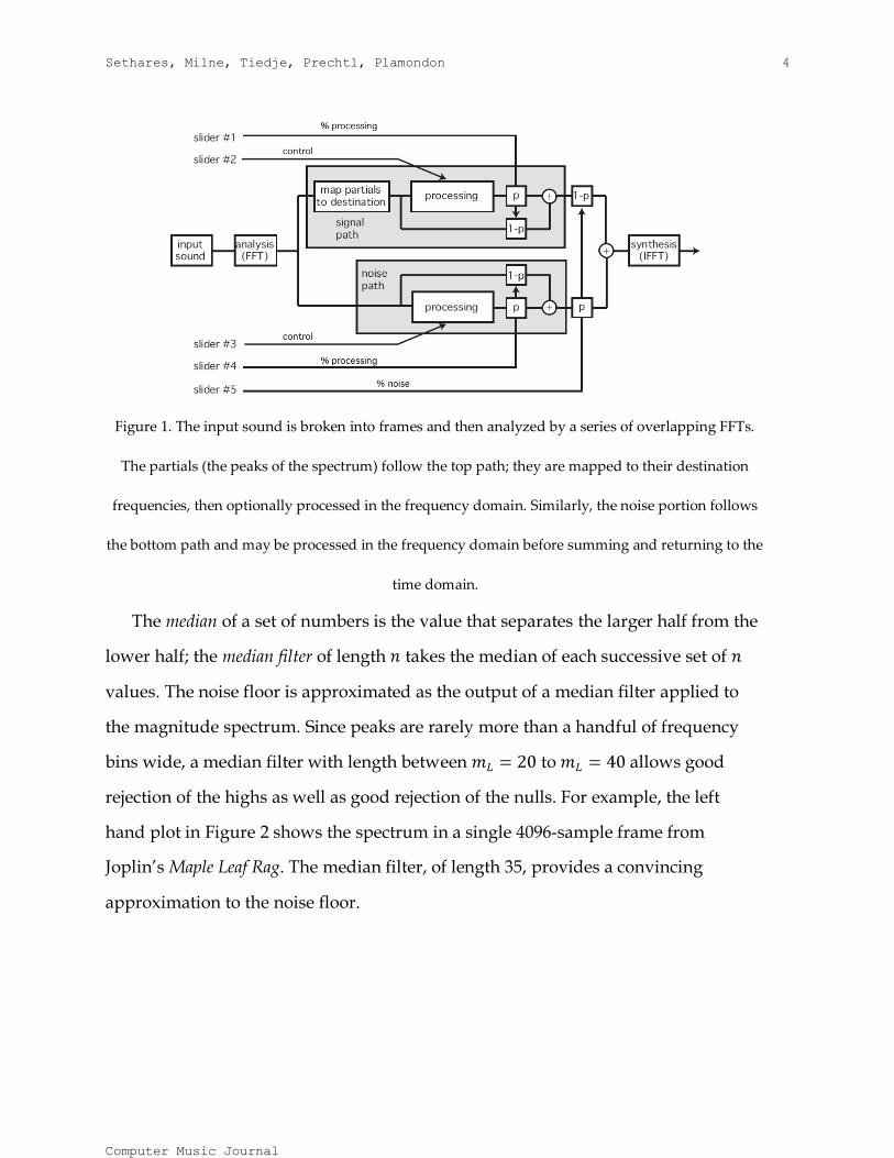
In order to individually manipulate the partials of a sound, it is necessary to

locate them. The Spectral Toolbox begins by separating the signal (the most

prominent tonal material) from the noise (rapid transients or other components that

are distributed over a wide range of frequencies). This allows the peaks to be treated

differently from the noise and the basic flow of information in all of the routines is

shown in Figure 1. This separation helps preserve the integrity of the tonal material

and helps preserve valuable impulsive information such as the attacks of notes that

otherwise may be lost due to smearing (Serra 1994).

http://www.cae.wisc.edu/~sethares/spectoolsCMJ.html




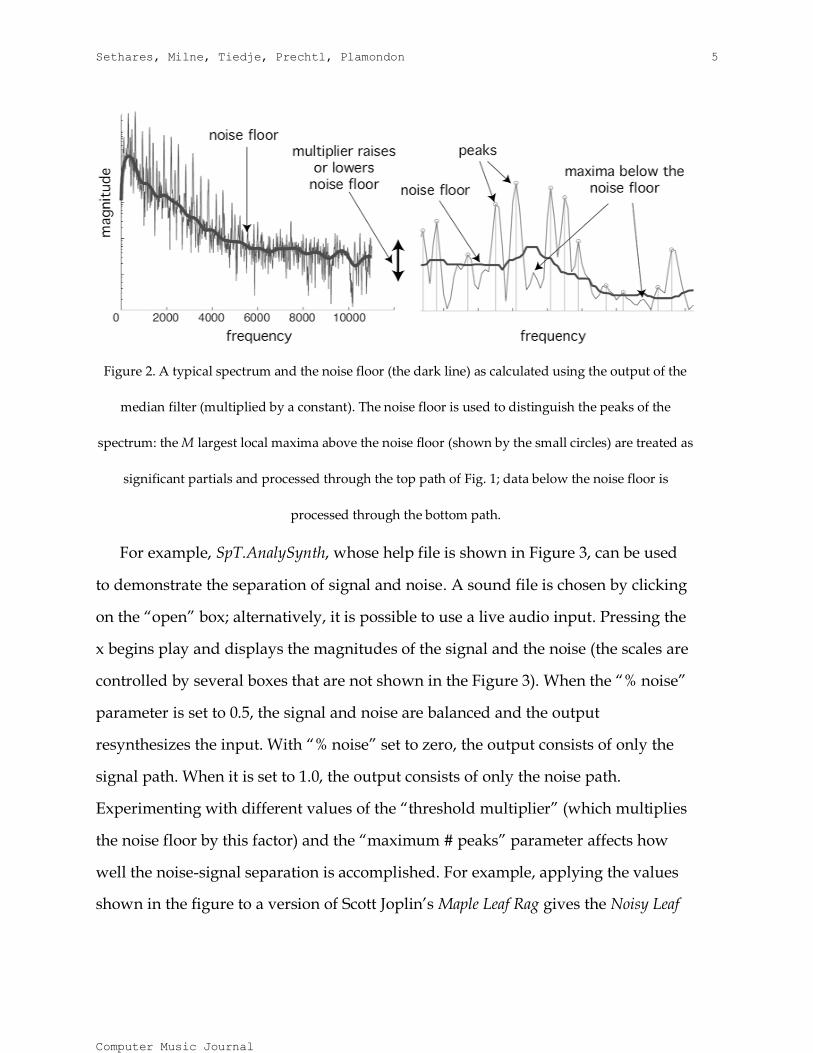
The median of a set of numbers is the value that separates the larger half from the

lower half; the median filter of length takes the median of each successive set of

values. The noise floor is approximated as the output of a median filter applied to

the magnitude spectrum. Since peaks are rarely more than a handful of frequency

bins wide, a median filter with length between to allows good

rejection of the highs as well as good rejection of the nulls. For example, the left

hand plot in Figure 2 shows the spectrum in a single 4096-sample frame from

Joplin‘s Maple Leaf Rag. The median filter, of length 35, provides a convincing

approximation to the noise floor.

Figure 1. The input sound is broken into frames and then analyzed by a series of overlapping FFTs.

The partials (the peaks of the spectrum) follow the top path; they are mapped to their destination

frequencies, then optionally processed in the frequency domain. Similarly, the noise portion follows

the bottom path and may be processed in the frequency domain before summing and returning to the

time domain.



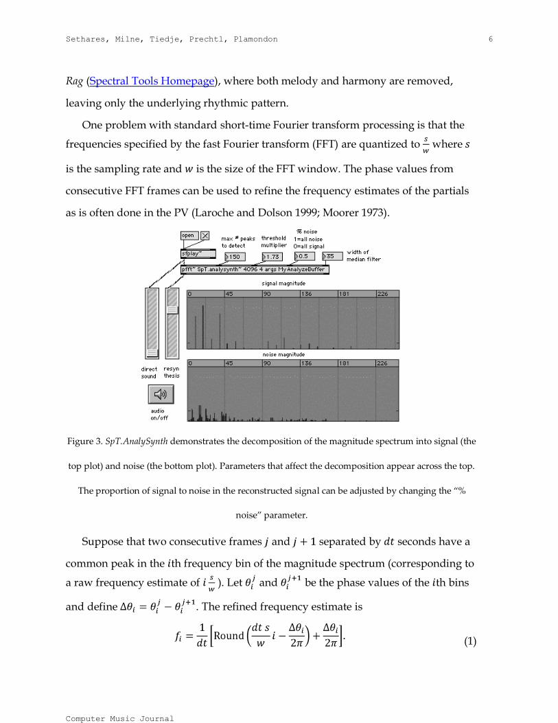
For example, SpT.AnalySynth, whose help file is shown in Figure 3, can be used

to demonstrate the separation of signal and noise. A sound file is chosen by clicking

on the ―open‖ box; alternatively, it is possible to use a live audio input. Pressing the

x begins play and displays the magnitudes of the signal and the noise (the scales are

controlled by several boxes that are not shown in the Figure 3). When the ―% noise‖

parameter is set to 0.5, the signal and noise are balanced and the output

resynthesizes the input. With ―% noise‖ set to zero, the output consists of only the

signal path. When it is set to 1.0, the output consists of only the noise path.

Experimenting with different values of the ―threshold multiplier‖ (which multiplies

the noise floor by this factor) and the ―maximum # peaks‖ parameter affects how

well the noise-signal separation is accomplished. For example, applying the values

shown in the figure to a version of Scott Joplin‘s Maple Leaf Rag gives the Noisy Leaf

Figure 2. A typical spectrum and the noise floor (the dark line) as calculated using the output of the

median filter (multiplied by a constant). The noise floor is used to distinguish the peaks of the

spectrum: the M largest local maxima above the noise floor (shown by the small circles) are treated as

significant partials and processed through the top path of Fig. 1; data below the noise floor is

processed through the bottom path.



Rag (Spectral Tools Homepage), where both melody and harmony are removed,

leaving only the underlying rhythmic pattern.

One problem with standard short-time Fourier transform processing is that the

frequencies specified by the fast Fourier transform (FFT) are quantized to where

is the sampling rate and is the size of the FFT window. The phase values from

consecutive FFT frames can be used to refine the frequency estimates of the partials

as is often done in the PV (Laroche and Dolson 1999; Moorer 1973).

Suppose that two consecutive frames and separated by seconds have a

common peak in the th frequency bin of the magnitude spectrum (corresponding to

a raw frequency estimate of ). Let and be the phase values of the th bins

and define . The refined frequency estimate is

(1)

Figure 3. SpT.AnalySynth demonstrates the decomposition of the magnitude spectrum into signal (the

top plot) and noise (the bottom plot). Parameters that affect the decomposition appear across the top.

The proportion of signal to noise in the reconstructed signal can be adjusted by changing the “%

noise” parameter.




The accuracy of this estimate has been shown to approach that of a maximum

likelihood estimate (the value of the frequency that maximizes the conditional

probability of given the data) for some choices of parameters (Puckette 1998). In

practice, the frequency values reported are significantly more accurate than the raw

frequency estimates.

Similarly, in the resynthesis step, the destination frequencies for the partials can

be specified to a much greater accuracy than by adjusting the frequencies of the

partials using phase differences in successive frames. To be explicit, suppose that the

frequency is to be mapped to some value . Let be the closest frequency bin in

the FFT vector (i.e., the integer that minimizes ). The th bin of the output

spectrum at time has magnitude equal to the magnitude of the th bin of the

input spectrum with corresponding phase

(2)

Spectral Mappings

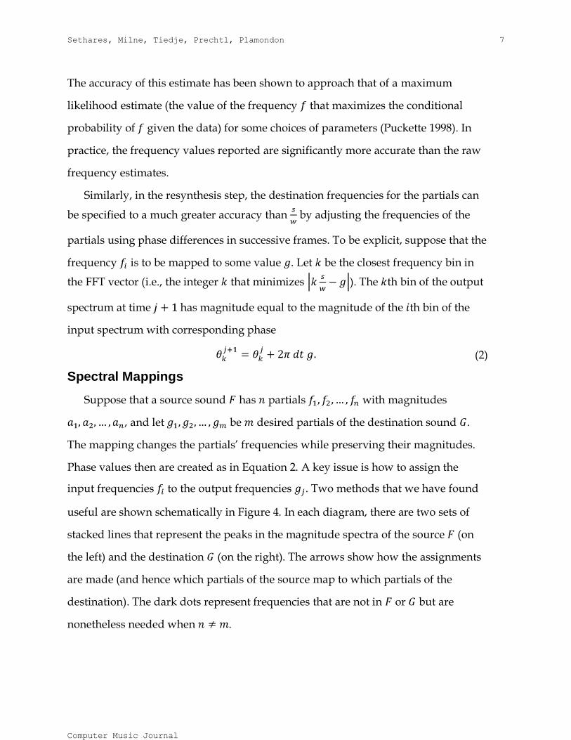
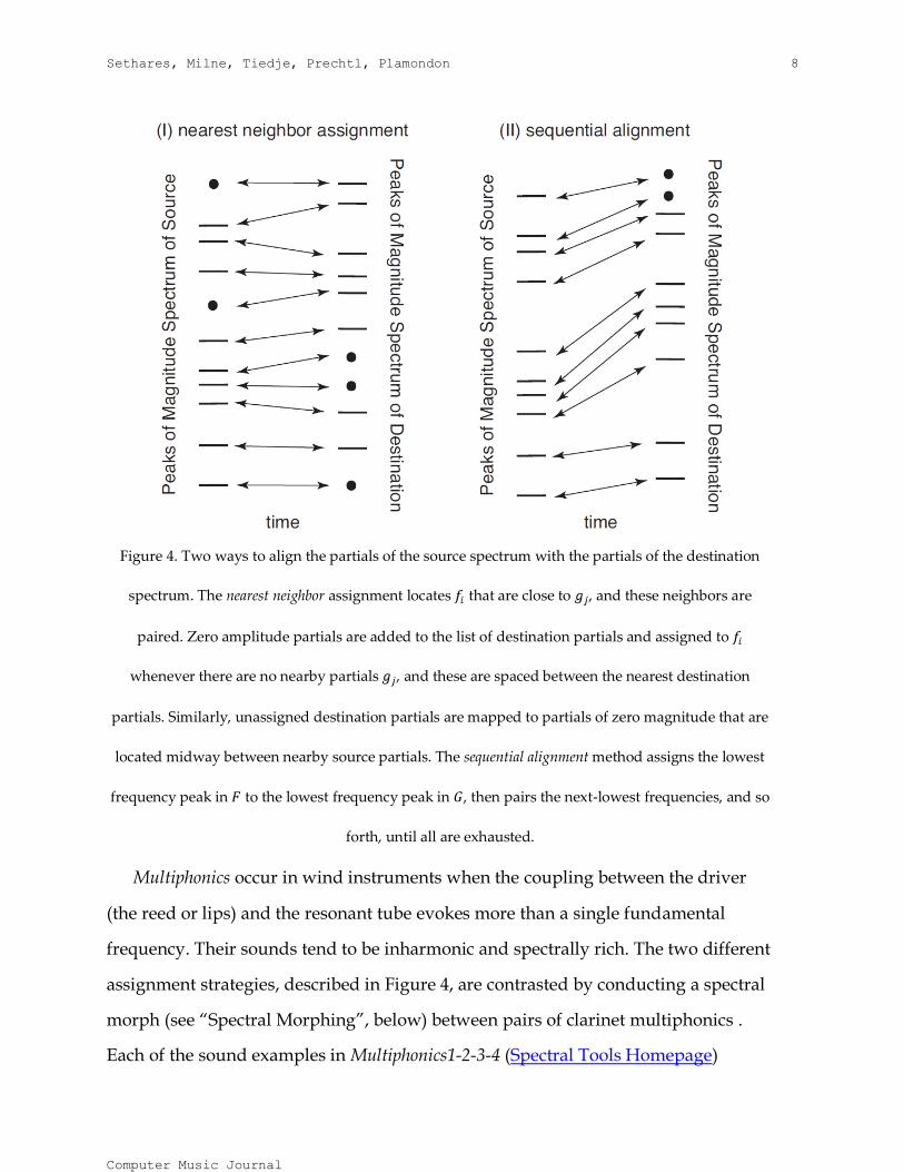
Suppose that a source sound has partials with magnitudes

, and let be desired partials of the destination sound .

The mapping changes the partials‘ frequencies while preserving their magnitudes.

Phase values then are created as in Equation 2. A key issue is how to assign the

input frequencies to the output frequencies . Two methods that we have found

useful are shown schematically in Figure 4. In each diagram, there are two sets of

stacked lines that represent the peaks in the magnitude spectra of the source (on

the left) and the destination (on the right). The arrows show how the assignments

are made (and hence which partials of the source map to which partials of the

destination). The dark dots represent frequencies that are not in or but are

nonetheless needed when .



Multiphonics occur in wind instruments when the coupling between the driver

(the reed or lips) and the resonant tube evokes more than a single fundamental

frequency. Their sounds tend to be inharmonic and spectrally rich. The two different

assignment strategies, described in Figure 4, are contrasted by conducting a spectral

morph (see ―Spectral Morphing‖, below) between pairs of clarinet multiphonics .

Each of the sound examples in Multiphonics1-2-3-4 (Spectral Tools Homepage)

Figure 4. Two ways to align the partials of the source spectrum with the partials of the destination

spectrum. The nearest neighbor assignment locates that are close to , and these neighbors are

paired. Zero amplitude partials are added to the list of destination partials and assigned to

whenever there are no nearby partials , and these are spaced between the nearest destination

partials. Similarly, unassigned destination partials are mapped to partials of zero magnitude that are

located midway between nearby source partials. The sequential alignment method assigns the lowest

frequency peak in to the lowest frequency peak in , then pairs the next-lowest frequencies, and so

forth, until all are exhausted.




presents two different multiphonics and then a 15 second morph between them. The

various assignment strategies can cause significant differences in the motion of the

sound. There are also other ways that the assignments might be made. For example,

the sequential alignment might begin with the highest, rather than the lowest,

partials. The partials with the maximum magnitudes might be aligned, followed by

those with the second largest, and so forth, until all are exhausted. Or, alternatively,

some important pair of partials might be identified (e.g., the largest in magnitude, or

the ones nearest the spectral centroid) and the others aligned sequentially above and

below. Early experiments suggest that many of these methods lead to erratic results

in which the pitch changes dramatically in response to small changes in the input

sound.

Applications of the Spectral Toolbox

The analysis, spectral mappings, and resynthesis processes described in the

previous sections enable a variety of routines including fixed spectral mappings

(sending all partials of a sound to fixed destinations), spectral morphing

(continuously interpolating between the partials of a source sound and a

destination) and Dynamic Tonality. These are described in the next few sections.

Fixed Destinations

Perhaps the most straightforward use of the spectral mapping technology is to

map the input to a fixed destination spectrum . For example, since harmonic

sounds play an important role in perception, might be chosen to be a harmonic

series built on a fundamental frequency (i.e., ) as implemented in the

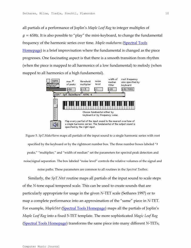
SpT.MakeHarm routine of Figure 5. A sound is played using sfplay and the root is

chosen either by typing into the rightmost number box or by clicking on the

keyboard (this can easily be replaced with a MIDI input). The input might be an

inharmonic sound such as a gong (see harmonicgong at Spectral Tools Homepage), or

it may be a full piece such as the 65 Hz Rag (Spectral Tools Homepage) which maps





all partials of a performance of Joplin‘s Maple Leaf Rag to integer multiples of

. It is also possible to ―play‖ the mini-keyboard, to change the fundamental

frequency of the harmonic series over time. Maple-makeharm (Spectral Tools

Homepage) is a brief improvisation where the fundamental is changed as the piece

progresses. One fascinating aspect is that there is a smooth transition from rhythm

(when the piece is mapped to all harmonics of a low fundamental) to melody (when

mapped to all harmonics of a high fundamental).

Similarly, the SpT.Ntet routine maps all partials of the input sound to scale steps

of the N-tone equal tempered scale. This can be used to create sounds that are

particularly appropriate for usage in the given N-TET scale (Sethares 1997) or to

map a complete performance into an approximation of the ―same‖ piece in N-TET.

For example, Maple5tet (Spectral Tools Homepage) maps all the partials of Joplin‘s

Maple Leaf Rag into a fixed 5-TET template. The more sophisticated Magic Leaf Rag

(Spectral Tools Homepage) transforms the same piece into many different N-TETs,

Figure 5. SpT.MakeHarm maps all partials of the input sound to a single harmonic series with root

specified by the keyboard or by the rightmost number box. The three number boxes labeled “#

peaks,” “multiplier,” and “width of median” set the parameters for spectral peak detection and

noise/signal separation. The box labeled “noise level” controls the relative volumes of the signal and

noise paths. These parameters are common to all routines in the Spectral Toolbox.








using different tuning mappings in a way that is somewhat analogous to the change

of chord patterns in a more traditional setting. The most general of the fixed

destination routines is SpT.Sieve, which maps the input sound to a collection of

partials specified by a user-definable table.

Spectral Morphing

Spectral morphing generates sound that moves smoothly between a source

spectrum and a destination spectrum over a specified time . Suppose that has

partials at with magnitude and has partials at

with magnitude . The two spectra are assumed to be aligned (using one of the

methods of Figure 4) so that both have the same number of entries . Let and

be the noise spectra of and . Let be 0 at the start of the morph and be 1 at time

. The morph then defines the spectrum at all intermediate times with log-spaced

frequencies

(3)

linearly-spaced intermediate magnitudes

(4)

and interpolated noise spectra

(5)

Logarithmic interpolation is used in Equation 3 because it preserves the

intervallic structure of the partials. The most common example is for harmonic

series. If the source and destination each consist of a harmonic series (and if the

corresponding elements are mapped to each other in the alignment procedure), then

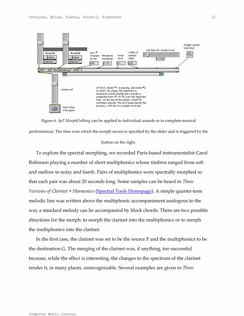
at every , the intervening sounds also have a harmonic structure. This is shown

mathematically in Appendix A and can be demonstrated concretely using

SpT.MorphOnBang, which appears in Figure 6.



To explore the spectral morphing, we recorded Paris-based instrumentalist Carol

Robinson playing a number of short multiphonics whose timbres ranged from soft

and mellow to noisy and harsh. Pairs of multiphonics were spectrally morphed so

that each pair was about 20 seconds long. Some samples can be heard in Three

Versions of Clarinet + Harmonics (Spectral Tools Homepage). A simple quarter-tone

melodic line was written above the multiphonic accompaniment analogous to the

way a standard melody can be accompanied by block chords. There are two possible

directions for the morph: to morph the clarinet into the multiphonics or to morph

the multiphonics into the clarinet.

In the first case, the clarinet was set to be the source F and the multiphonics to be

the destination G. The merging of the clarinet was, if anything, too successful

because, while the effect is interesting, the changes to the spectrum of the clarinet

render it, in many places, unrecognizable. Several examples are given in Three

Figure 6. SpT.MorphOnBang can be applied to individual sounds or to complete musical

performances. The time over which the morph occurs is specified by the slider and is triggered by the

button on the right.




Versions of Clarinet + Harmonics . The first plays the unaccompanied melody. The

next three morph that same line into various sets of multiphonics.

In the second case, a Max/MSP patch is used to ―listen‖ to the melody and

choose which multiphonics to play at each instant. The score calls for significant

microtonal improvisation by the clarinet player, and the software chooses, retunes,

and morphs the multiphonics on-the-fly to create an unusual inharmonic backdrop.

The Legend of Spectral Phollow premiered at CCMIX in Paris on July 13, 2006. Carol

Robinson played the clarinet, and William Sethares ―played‖ the software. A

recording of this performance can be heard at Legend (Spectral Tools Homepage).

Dynamic Tonality

There are many possible tunings: equal temperaments, meantones, circulating

temperaments, various forms of just intonation, and so forth. Each seems to require

a different method of playing and a different interface, necessitating significant time

and effort to master. In (Milne, Sethares, and Plamondon 2007, 2008), we introduced

a way of parameterizing tunings so that many seemingly unrelated systems can be

performed on one keyboard with the same fingerings for the same chords and

melodies; this is called tuning invariance. For example, the Syntonic continuum

begins at 7-TET, moves through 19-TET, a variety of meantone tunings, 12-TET, 17-

TET, 22-TET and on up to 5-TET (as shown on the main tuning slider in Figure 7).

On a musical controller with a two-dimensional array of keys, a chord or melody

can usually be fingered the same throughout all the tunings of this continuum.

The TransFormSynth, which is implemented using the same audio routines as

described in the Spectral Toolbox, realizes these methods and extends them in two

ways. First, the tuning can be moved towards a nearby just intonation. Second, the

spectrum of the sound can be tempered along with the tuning. Both of these

temperings are implemented using the Tone Diamond—a convenient two-




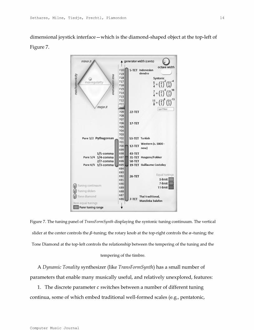
dimensional joystick interface—which is the diamond-shaped object at the top-left of

Figure 7.

A Dynamic Tonality synthesizer (like TransFormSynth) has a small number of

parameters that enable many musically useful, and relatively unexplored, features:

1. The discrete parameter switches between a number of different tuning

continua, some of which embed traditional well-formed scales (e.g., pentatonic,

Figure 7. The tuning panel of TransFormSynth displaying the syntonic tuning continuum. The vertical

slider at the center controls the -tuning; the rotary knob at the top-right controls the –tuning; the

Tone Diamond at the top-left controls the relationship between the tempering of the tuning and the

tempering of the timbre.



diatonic, chromatic), and some of which embed radically different well-formed

scales (e.g., scales with 3 large steps and 7 small steps per octave).

2. The continuous parameters , , and move the tuning between a number of

equal temperaments (e.g., 7-TET, 31-TET, 12-TET, 17-TET, and 5-TET), non-equal

temperaments (e.g. quarter-comma meantone, and Pythagorean), circulating

temperaments, and closely-related just intonations.

3. The continuous parameter moves the timbre from being perfectly harmonic

to being perfectly matched to the tuning, thus minimizing sensory dissonance

(Sethares 1993).

4. The mapping to a two-dimensional lattice of buttons and on a musical

controller provides the same fingering pattern for all tonal intervals across all

possible keys and tunings within any given continuum (Milne, Sethares, and

Plamondon 2008).

Each of these parameters is defined and explained in more depth in the following

subsections.

Generator Tunings ( and ) and Note Coordinates ( and )

Invariant fingering over a tuning continuum requires a linear mapping of the notes

of a higher-dimensional just intonation to the notes of a one or two-dimensional

temperament (such as 12-TET or quarter-comma meantone), and a linear mapping

of these tempered notes to a two-dimensional array of buttons or keys on a musical

controller. Perhaps the simplest way to explain the system is by example. A -limit

just intonation contains intervals tuned to ratios that can be factorized by prime

numbers up to, but no higher than, . Consider 11-limit just intonation (in which

), which consists of all the intervals generated by integer multiples of the

primes 2, 3, 5, 7, and 11. Thus simple intervals, such as the just fifth or just major

third, can be represented as the frequency ratios and ,

respectively, while a less simple interval such as the just major seventh (a perfect



fifth plus a major third) is A comma , is a set of

integers that tempers (changes the numerical values of) the generators so that

. For example, the well-known syntonic comma, which can be

written in fractional form as , is represented by since it is equal to

. A system of commas can be represented by a matrix of integer

values, so the commas , ,

, can be represented as the matrix ,

which has a null space (kernel) , where T is the

transpose operator. This matrix is transposed and then written in row-reduced

echelon form to give the transformation matrix . Using

, the matrix transforms any interval

into a similarly sized (i.e., tempered) interval . A basis (i.e., a set of vectors

that can, in linear combination, represent every vector in that space) for the

generators can be found by inspection of the columns of as , ,

, , and . Thus every interval in the

continuum (this is the 11-limit Syntonic continuum shown in Figure 7) can be

represented as integer powers of the two generators and —that is, as . For

further information and examples, see Milne, Sethares, and Plamondon (2008).

This means that if and are mapped to a basis of a button lattice (i.e.,

), such as the Thummer‘s (Figure 8), then the fundamental

frequency of any button of coordinate with respect to that basis, is given by

(6)

where is the frequency of the reference note. By default the reference note , on

which the pitches of all other notes are based, is D3 (whose concert pitch is

146.83Hz).



In the Syntonic continuum, the value of is near 2 and can be adjusted by the

rotary knob labeled ―octave width‖ at the top-right of Figure 7; the value of is near

1.5 and is specified by the main tuning slider. Altering the -tuning while playing

allows a keyboard performer to emulate the dynamic tuning of string and

aerophone players who prefer Pythagorean (or higher) tunings when playing

expressive melodies, quarter-comma meantone when playing consonant harmonies,

and 12-TET when playing with fixed pitch instruments such as the piano (Sundberg

1989).

Related Just Intonations ( )

The vertical dimension of the Tone Diamond (at the top-left of Figure 7) alters the

tuning in a different way—by moving it towards a related 5-limit just intonation.

Just intonations contain many intervals tuned to small number ratios (e.g., 3:2, 4:3,

5:4, 6:5, 7:5, 7:6, etc.), and these intervals are typically thought to be maximally

consonant and ―in tune‖ when using sounds with harmonic spectra. For this reason,

just intonation has been frequently cited as an ideal tuning (e.g., by Helmholtz

(1954), Partch (1974), and Mathieu (1997)). However, 5-limit just intonation is three-

dimensional, and higher-limit JI‘s have even more dimensions, making it all but

Figure 8. The coordinates of the Thummer's button lattice, when using its default Wicki note

layout (Milne, Sethares, and Plamondon 2008).



impossible to avoid ―wolf‖ intervals when mapping to a fixed pitch instrument

(Milne, Sethares, and Plamondon 2007).

Deciding precisely which JI ratios should be used also presents an issue, because

there is always ambiguity about precisely which JI interval is represented by a

tempered interval (because the mapping matrix is many-to-one, any ―reverse-

mapping‖ is somewhat ambiguous). For this reason we provide two aesthetically

motivated choices: ―Major JI‖, at the bottom of the diamond, maximizes the number

of justly tuned major triads (of ratio 4:5:6); while ―Minor JI‖, at the top of the

diamond, maximizes the number of justly tuned minor triads (of ratio 10:12:15).

The major and minor JI tuning ratios (relative to the reference note) for every

note are stored in a table. The major JI values are used when the control dot is

in the lower half of the Tone Diamond (i.e., ), the minor JI values are

used when the control dot is in the upper half of the Tone Diamond (i.e.,

). Every different tuning continuum requires a different set of values. The vertical

dimension of the Tone Diamond controls how much the tuning is moved towards

these JI values, denoted , using the formula , where

is the position of the control dot on the Tone Diamond‘s -axis. This means the

frequency of any note can be calculated accordingly:

(7)

The Tone Diamond and main tuning slider, therefore, facilitate dynamic tuning

changes between many different tuning systems. When the Tone Diamond‘s control

point is anywhere along the central horizontal line (the ―Max. Regularity‖ line), the

tuning is a regular one- or two-dimensional tuning such as 12-TET or quarter-

comma meantone, as shown on the main tuning slider. When the control point is

moved upwards or downwards the tuning moves towards a related just intonation.

The tunings that are intermediate between perfect regularity and JI are like the



circulating temperaments of Kirnberger and Vallotti in that every key has a (slightly)

different tuning. And all of these tunings have essentially the same fingering when

played on a 2-D lattice controller.

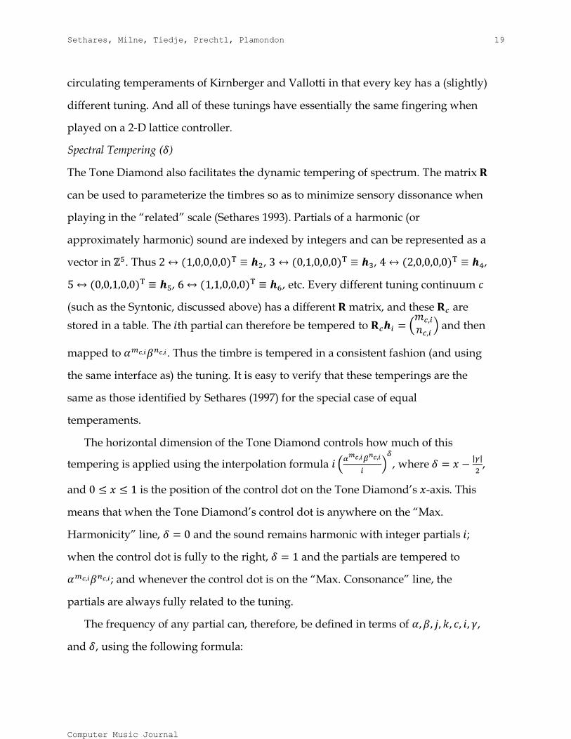
Spectral Tempering ( )

The Tone Diamond also facilitates the dynamic tempering of spectrum. The matrix

can be used to parameterize the timbres so as to minimize sensory dissonance when

playing in the ―related‖ scale (Sethares 1993). Partials of a harmonic (or

approximately harmonic) sound are indexed by integers and can be represented as a

vector in . Thus , , ,

, , etc. Every different tuning continuum

(such as the Syntonic, discussed above) has a different matrix, and these are

stored in a table. The th partial can therefore be tempered to and then

mapped to . Thus the timbre is tempered in a consistent fashion (and using

the same interface as) the tuning. It is easy to verify that these temperings are the

same as those identified by Sethares (1997) for the special case of equal

temperaments.

The horizontal dimension of the Tone Diamond controls how much of this

tempering is applied using the interpolation formula , where ,

and is the position of the control dot on the Tone Diamond‘s -axis. This

means that when the Tone Diamond‘s control dot is anywhere on the ―Max.

Harmonicity‖ line, and the sound remains harmonic with integer partials ;

when the control dot is fully to the right, and the partials are tempered to

; and whenever the control dot is on the ―Max. Consonance‖ line, the

partials are always fully related to the tuning.

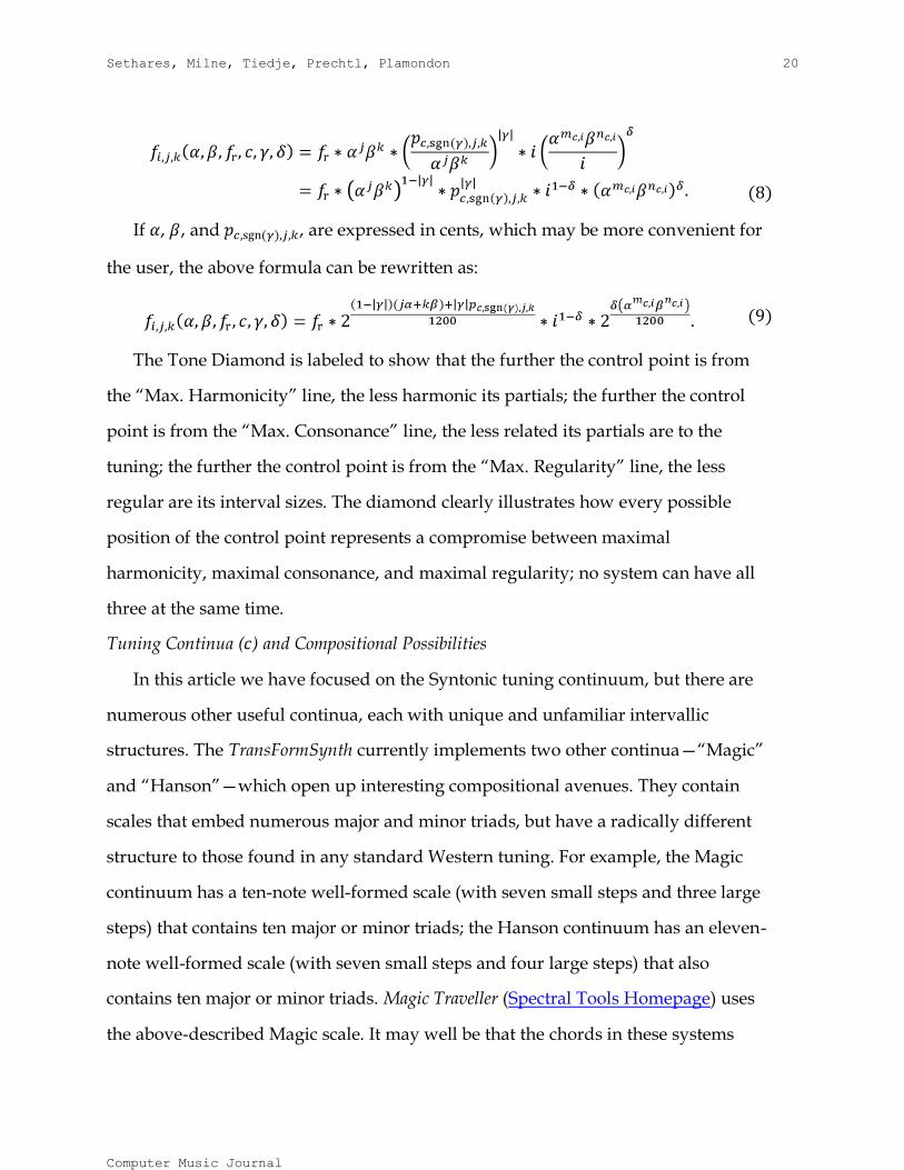
The frequency of any partial can, therefore, be defined in terms of ,

and , using the following formula:



(8)

If , , and , are expressed in cents, which may be more convenient for

the user, the above formula can be rewritten as:

(9)

The Tone Diamond is labeled to show that the further the control point is from

the ―Max. Harmonicity‖ line, the less harmonic its partials; the further the control

point is from the ―Max. Consonance‖ line, the less related its partials are to the

tuning; the further the control point is from the ―Max. Regularity‖ line, the less

regular are its interval sizes. The diamond clearly illustrates how every possible

position of the control point represents a compromise between maximal

harmonicity, maximal consonance, and maximal regularity; no system can have all

three at the same time.

Tuning Continua ( ) and Compositional Possibilities

In this article we have focused on the Syntonic tuning continuum, but there are

numerous other useful continua, each with unique and unfamiliar intervallic

structures. The TransFormSynth currently implements two other continua—―Magic‖

and ―Hanson‖—which open up interesting compositional avenues. They contain

scales that embed numerous major and minor triads, but have a radically different

structure to those found in any standard Western tuning. For example, the Magic

continuum has a ten-note well-formed scale (with seven small steps and three large

steps) that contains ten major or minor triads; the Hanson continuum has an eleven-

note well-formed scale (with seven small steps and four large steps) that also

contains ten major or minor triads. Magic Traveller (Spectral Tools Homepage) uses

the above-described Magic scale. It may well be that the chords in these systems




have functional relationships that are quite different to those found in standard

diatonic/chromatic tonality. Such systems, therefore, open up the possibility of an

aesthetic research program similar to that which may be said to have characterized

the development of common-practice from the birth of harmonic tonality in the

sixteenth century to the ―crisis of tonality‖ at the end of the nineteenth.

But the well-structured tonal relationships found in these continua do not

support only a strictly tonal compositional style. Serial (and other ―atonal‖)

compositional techniques are just as applicable to these alternative continua, as are

techniques which explore the implications of unusual timbral combinations and

structures. Each continuum offers a unique set of mathematical possibilities and

constraints. For example, the familiar 12-note division of the octave has many factors

(2, 3, 4, and 6), thus enabling interval classes of these sizes to cycle back to the

starting note, and modes of limited transposition to be formed. Conversely, a 13-

note division of the octave, which can be made to sound quite ―in-tune‖ when the

spectrum is tempered to the Magic continuum, has no factors and so contains no

modes of limited transposition and no interval cycles. The 15-note division found in

Hanson has factors of 3 and 5, suggesting a quite different set of structural

possibilities. ChatterBar and Lighthouse (Spectral Tools Homepage) are both non-

serial ―atonal‖ pieces—in 53-TET Syntonic and 11-TET Hanson, respectively.

Alongside these structural possibilities are the dynamic variations in tuning and

timbre that can be easily controlled (and even notated) with the , , , and

parameters. Smooth changes of tuning and timbre are at the core of C2ShiningC ,

while in Shred (Spectral Tools Homepage), the music switches from 12-TET to 5-TET

Syntonic.

Dynamic Tonality, therefore, opens up a rich set of compositional possibilities of

both depth and simplicity.





Discussion

The analysis-resynthesis method utilized by the Spectral Toolbox allows the

independent control of both frequency and amplitude for every partial in a given

sound. However, since a typical musical sound consists of tens or even hundreds of

audible partials, it is apparent that their individual manipulation is not necessarily

practical. In order to reduce information load and retain musical relevance, there is

need for an organizational routine which parameterizes spectral information in a

simple and musically meaningful interface. The Spectral Toolbox has addressed this

problem by providing three different routines: (1) mapping partials to a fixed

destination, (2) morphing between different spectra, and (3) Dynamic Tonality.

Though we have so far only discussed the reconstruction of preexisting sounds,

it is also possible to manipulate the harmonic information of purely synthesized

sound. The ideas presented in this paper are applicable to virtually any synthesis

method that allows complete control over harmonic information. For example, The

Viking (Milne and Prechtl, 2008) is an additive synthesizer which implements

Dynamic Tonality in the same manner as the TransFormSynth, except that it

synthesizes each partial with its own sinusoidal oscillator. Similarly, The Synth O’

Nine Filters (Prechtl and Milne, 2009) uses modal synthesis to implement Dynamic

Tonality in a physical modeling algorithm. In this case, a noise loop or burst is fed

through a series of resonant filters that represent specific partials through their

individual feedback coefficients.

There are benefits pertaining to each of these synthesis methods: additive

synthesis is, relatively speaking, computationally efficient, while modal synthesis, at

the cost of greater computational power, enables realistic and dynamic physical

modeling. However, the analysis-resynthesis method is interesting because it

enables the harmonic manipulation of any sound, and can do so for both fixed and

live audio inputs. This means that, given its relatively simple user interface, the



Spectral Toolbox has the capacity to provide novel and worthwhile approaches to

computer music composition and performance. The musical examples available on

the website should hopefully provide at least some indication of these new artistic

possibilities.

Beyond the artistic benefits described above, there are also strong implications

for music research, particularly in the area of cognition. The mutual control of

tuning and timbre facilitates a deeper examination of the musical ramifications that

such a relationship entails. Perhaps of greatest interest is how formerly inaccessible

(that is, in an aesthetic sense) tunings may be rendered accessible through the

timbral manipulations described above. Such an idea calls for further research

regarding varying forms of dissonance—most notably melodic dissonance (Van der

Merwe 1992; Weisethaunet 2001)—and harmonic tonality in general. It seems likely,

especially with the Spectral Toolbox, that such concepts will soon need to take

alternate tunings into account. In fact, the widespread use of microtonality in

electro-acoustic composition, performance, and research seems much closer now

than it ever has.

Acknowledgements

The authors would like to thank Gerard Pape for helpful discussions, and Carol

Robinson for the excellent performance of Legend.

References

Carlos, W. 1987. ―Tuning: At the Crossroads.‖ Computer Music Journal 11(1):29–43.

Carlos, W. 1987. Secrets of Synthesis. CBS Records MK 42333.

Dolson, M. 1986. ―The Phase Vocoder: A Tutorial.‖ Computer Music Journal 10(4):14–

27.

Helmholtz, H. L. F. 1954. On the Sensations of Tone. New York: Dover.

Laroche, J., and M. Dolson. 1999. ―Improved Phase Vocoder Time-scale Modification

of Audio.‖ IEEE Trans. on Audio and Speech Processing 7(3).



Cycling ‘74. Max/MSP Reference Manual. Available online at www.cycling74.com.

Mathieu, W. A. 1997. Harmonic Experience. Rochester: Inner Traditions International.

Milne, A., and A. Prechtl. 2008. The Viking. Available online at

www.dynamictonality.com.

Milne, A., W. A. Sethares, and J. Plamondon. 2007. ―Isomorphic Controllers and

Dynamic Tuning: Invariant Fingering over a Tuning Continuum.‖ Computer

Music Journal 31(4):15–32.

Milne, A., W. A. Sethares, and J. Plamondon. 2008. ―Tuning Continua and Keyboard

Layouts.‖ Journal of Mathematics and Music 2(1):1–19.

Moorer, J. A. 1973. ―The Use of the Phase Vocoder in Computer Music

Applications.‖ Journal of the Audio Engineering Society 26(1/2):42–45.

Partch, H. 1974. Genesis of a Music. New York: Da Capo Press.

Prechtl, A., and A. Milne. 2009. The Synth O’ Nine Filters. Available online at

www.dynamictonality.com.

Puckette, M. S., and J. C. Brown. 1998. ―Accuracy of Frequency Estimates Using the

Phase Vocoder.‖ IEEE Trans. Speech and Audio Processing 6(2).

Serra, X. 1994. ―Sound Hybridization Based on a Deterministic plus Stochastic

Decomposition Model.‖ In Proceedings of the 1994 International Computer Music

Conference, Aarhus, Denmark, 348351.

Sethares, W. A. 1993. ―Local Consonance and the Relationship between Timbre and

Scale.‖ Journal of the Acoustical Society of America 94(3):1218–1228.

Sethares, W. A. 1998. ―Consonance-based Spectral Mappings.‖ Computer Music

Journal 22(1):56–72.

Sethares, W. A. 2004. Tuning, Timbre, Spectrum, Scale, 2nd ed. London: Springer-

Verlag.

Sundberg, J., A. Friberg, and L. Frydén. 1989. ―Rules for Automated Performance of

Ensemble Music,‖ Contemporary Music Review 3(1):89–109.

http://www.cycling74.com/

http://www.dynamictonality.com/

http://www.dynamictonality.com/



Van der Merwe, P. 1992. Origins of the Popular Style. Oxford: Clarendon Press.

Weisethaunet, H. 2001. ―Is There Such a Thing as the ‗Blue Note‘?‖Popular Music

20(1):99–116.

Appendix A: Preservation of Intervallic Structure Under

Logarithmic Interpolation

Suppose that the source peaks and the destination peaks have the same

intervallic structure, i.e., that

(10)

for . Morphing the two sounds using the logarithmic method

(Equation 3) creates a collection of intermediate sounds with peaks at

(11)

Then for every , the intervallic structure in the is the same as that in

the source and destination. To see this, observe that

(12)

The last equality follows directly from Equation 10. In particular, if the and are

the partials of harmonic sounds (though perhaps with different magnitudes and

different fundamentals) then the interpolated sounds are also harmonic, with

spectra that smoothly connect and and with fundamental frequency (and hence,

most likely, with pitch) that moves smoothly from that of to that of .

spectral tools for dynamic tonality and audio morphing

Documents