Spectroscopic Evidence for a Temperature Inversion in the

Dayside Atmosphere of the Hot Jupiter WASP-33b

Korey Haynes1,2,6, Avi M. Mandell1, Nikku Madhusudhan3, Drake Deming4 , Heather

Knutson5

ABSTRACT

We present observations of two occultations of the extrasolar planet WASP-

33b using the Wide Field Camera 3 (WFC3) on the HST, which allow us to

constrain the temperature structure and composition of its dayside atmosphere.

WASP-33b is the most highly irradiated hot Jupiter discovered to date, and

the only exoplanet known to orbit a δ-Scuti star. We observed in spatial scan

mode to decrease instrument systematic effects in the data, and removed fluc-

tuations in the data due to stellar pulsations. The RMS for our final, binned

spectrum is 1.05 times the photon noise. We compare our final spectrum, along

with previously published photometric data, to atmospheric models of WASP-

33b spanning a wide range in temperature profiles and chemical compositions.

We find that the data require models with an oxygen-rich chemical composition

and a temperature profile that increases at high altitude. We also find that our

spectrum displays an excess in the measured flux towards short wavelengths that

is best explained as emission from TiO. If confirmed by additional measurements

at shorter wavelengths, this planet would become the first hot Jupiter with a

temperature inversion that can be definitively attributed to the presence of TiO

in its dayside atmosphere.

Subject headings: stars: planetary systems - eclipses - techniques: photometric -

techniques: spectroscopic

1Solar System Exploration Division, NASA Goddard Space Flight Center, Greenbelt, MD 20771, USA

2School of Physics, Astronomy, and Computational Sciences, George Mason University, Fairfax, VA 22030,

USA

3Institute of Astronomy, University of Cambridge, Cambridge CB3 0HA, UK

4Department of Astronomy, University of Maryland, College Park, MD 20742, USA

5Division of Geological & Planetary Sciences, California Institute of Technology, Pasadena, CA 91125,

USA

6Corresponding Email: khaynes0112@gmail.com

arX

iv:1

505.

0149

0v1

[as

tro-

ph.E

P] 6

May

201

5

– 2 –

1. Introduction

One of the most intriguing areas of study in the field of exoplanet characterization is

the temperature structure of exoplanet atmospheres. Hot Jupiters represent an extreme end

of the exoplanet distribution: they orbit very close to their host stars, which subjects them

to an intense amount of stellar radiation. Also due to their proximity, they likely become

tidally locked on astrophysically short timescales (Guillot et al. 1996), and are heated only

on the side facing the star. This results in strong zonal winds (Showman et al. 2008) that

redistribute the heat, with the dynamics of this redistribution dictated by the physical and

thermal structure of the planet’s atmosphere.

Temperature inversions were an early prediction from atmospheric models of highly

irradiated planets (Hubeny et al. 2003; Fortney et al. 2008), which demonstrated that strong

absorption of incident UV/visible irradiation by high-temperature absorbers such as TiO and

VO, which are commonly found in low-mass stars and brown dwarfs, could lead to thermal

inversions in their observable atmospheres. Evidence for the existence of thermal inversions

began with the first secondary eclipse measurements of HD209458b taken with the IRAC

camera on Spitzer by Knutson et al. (2008), who measured larger eclipse depths in spectral

regions with higher opacity due to features of H2O and CO (4.5 and 5.6 µm) compared with

nearby bands measuring the deeper thermal continuum (3.6 and 8 µm). However, more

recent analyses of HD209458b by Diamond-Lowe et al. (2014) and Schwarz et al. (2015)

do not support an inverted atmophere model; additionally, indications for the presence

or absence of an inversion in other planets based on Spitzer/IRAC data appear to defy

predictions based on the level of incident radiation or the overall equilibrium temperature of

the atmosphere (Machalek et al. 2008; Fressin et al. 2010, and others). More recent models

have suggested that heavy molecules such as TiO and VO may not remain suspended in

the upper atmosphere of Jupiter-mass planets (Spiegel et al. 2009), and searches for specific

spectral signatures of TiO in the optical have been unsuccessful (Sing et al. 2013; but see

also Hoeijmakers et al. 2014 for discussion of incompleteness in the TiO line list contributing

to inabilities to confirm observational detections). Recent theories have postulated several

additional atmospheric processes that could play a role in the formation of inversions, such as

the production of photochemical sulfur-based hazes (Zahnle et al. 2009) or the inhibition of

oxide formation due to a super-solar C/O ratio (Madhusudhan 2012). Furthermore, Knutson

et al. (2010) explored the possibility that the absorbing molecular species may be destroyed

by photodissociation and may, hence, be affected by the activity of the host star.

Progress on understanding the origin and conditions required for temperature inversions

has been further hampered by a lack of high-quality data for most sources. Only a single

unambiguous spectrally resolved measurement of a molecular feature in the eclipse spectrum

– 3 –

of a planet, the detection of water absorption in the WFC3 spectrum of WASP-43 b by Krei-

dberg et al. (2014), has been published to date. Eclipse measurements for most transiting

exoplanets comprise only the broadband Spitzer/IRAC filters, making the conclusions largely

model-dependent and subject to possible systematic offsets or uncertainties. The inference of

thermal inversions from IR photometry is based solely on our ability to determine whether

there is a larger-than-expected flux from molecular bands compared with the continuum.

Warm Spitzer photometry has now measured two-band eclipse depths for a large number of

planets, but while these measurements can provide some indication of a potential inversion,

such data cannot uniquely identify inverted atmospheres because of degeneracies between

atmospheric composition and structure (Madhusudhan & Seager 2010; Stevenson et al. 2010;

Moses et al. 2013). In particular, Madhusudhan & Seager (2010) showed that with only a

few data points, this interpretation is heavily dependent on the assumed composition of the

planet and the accuracy of the uncertainties ascribed to each measurement. A subsequent

Bayesian retrieval analysis on a subset of well-observed planets covering a wide range of

effective temperatures by Line & Yung (2013) showed that the data are inconsistent with

thermal inversions for many of the planets expected to have an inversion due to the afore-

mentioned theories for the physical origin of the phenomenon. More recently, a new analysis

by Diamond-Lowe et al. (2014) and Schwarz et al. (2015) revealed that a thermal inversion

is not necessary to explain the Spitzer observations of HD 209458b, previously considered

the prototypical example of a planet with an inverted atmosphere. Hansen et al. (2014) has

also suggested that the uncertainties on many older, single-visit Spitzer eclipse depths may

be significantly higher than previously reported, resulting in data sets that are essentially

consistent with featureless blackbody spectra.

It is therefore critical that we further investigate planets that provide the best chance

for confirming the presence of temperature inversions, in order to better constrain the actual

temperature structure of these planets and clarify the role of various stellar and planetary

characteristics in defining this structure. Here we present new secondary eclipse (or occul-

tation) observations of WASP-33b, one of the largest and hottest planets known, using the

Wide Field Camera 3 (WFC3) on HST. WASP-33 is an A-type δ-Scuti star and its planet,

WASP-33b, is one of the most highly irradiated planets discovered to date, orbiting once

every 1.22 days (Cameron et al. 2010; Herrero et al. 2011). WASP-33b is unique, being

the only exoplanet yet discovered to orbit a δ-Scuti star. Multiple observations of the host

star over wavelengths ranging from the visible to the infrared have shown oscillations with a

range of frequencies, and amplitudes on the order of 1 mmag. Given the extreme irradiation

received by WASP-33b, it is one of the most likely hot Jupiters to host a thermal inversion as

TiO/VO, if present, would be expected to be in the gaseous phase throughout the observable

dayside atmosphere, thereby causing a thermal inversion.

– 4 –

Previous occultation observations in the infrared (Deming et al. 2012) concluded that

WASP-33b might host a temperature inversion with a solar composition atmosphere, or a

non-inverted atmosphere with enhanced carbon abundance. The inversion scenario is advo-

cated by de Mooij et al. (2013), based on WASP-33b’s apparent inefficient heat redistribution,

which was also noted by Smith et al. (2011). Our spectroscopic observations with WFC3

cover a wavelength range from 1.1 to 1.7 µm, which provides a valuable opportunity to con-

firm the presence of an inversion in WASP-33b. The WFC3 spectral range covers strong

infrared molecular bands of H2O and TiO, both of which are expected to be abundant in

the atmosphere of WASP-33b, assuming a solar abundance composition. Assuming these

molecules contribute significant opacity at the height of the thermal inversion, the presence

of a thermal inversion would lead to emission features in the dayside spectrum due to both

these molecules in the WFC3 range, as opposed to absorption features if no thermal inversion

is present.

We describe the observations in Section 2, data reduction in Section 3, removal of stellar

oscillations and analysis strategies in Section 4, and discussion of results in Section 5.

2. Observations

Two occultations of WASP-33 were observed on November 25, 2012 and January 14,

2013. We used WFC3’s infrared G141 grism, which provides slitless spectra from 1.1µm to

1.7µm at a resolving power of 130 (Dressel 2012). Each target was allocated 5 HST orbits,

which was sufficient to cover a single planetary occultation while including periods of the

orbit both before and after occultation.

Both sets of observations were taken using the 256 x 256 sub-array with 7 non-destructive

reads per exposure, using the RAPID sampling sequence. The data were observed in spatial

scan mode (McCullough & MacKenty 2012), which increases the photon collection efficiency

of the detector, and additionally has been shown to decrease systematic patterns in the

data that can result from persistent levels of high flux on individual pixels. All scans were

performed in the same direction. See Table 1 for details.

3. Data Reduction

We used the series of single-exposure “ima” images produced by the WFC3 calwf3

pipeline for our data analysis. The “ima” files are fully reduced data products with the

exception of a step to combine multiple reads. The final stage “flt” files provided by the

– 5 –

Space Telescope Science Institute are not appropriate for use in spatial scan mode, since

the additional pipeline processing for combining multiple reads does not account for the

motion of the source on the detector in spatial scan mode. We followed the methodology of

Deming et al. (2013) to produce 2D spectral frames from the “ima” files provided on MAST.

We began by applying a top-hat mask in the spatial dimension of each read, the width of

which is 20 pixels tall in order to fully cover the stellar PSF. Areas outside the mask were

zeroed. We then subtracted subsequent reads, and then added the differenced frames to

create one scanned image. We used our own strategy from Mandell et al. (2013) to search

for and correct bad pixels within the combined spectral frames, and collapse the images

into 1D spectra. We used the modified coefficients from Wilkins et al. (2014) to produce

the wavelength and wavelength-dependent flat-field calibrations. For background correction,

we subtracted a single background value from each difference pair in the WASP-33 “ima”

files before applying the top-hat mask. The background subtraction decreases the overall

flux level of each light curve, thereby increasing the measured eclipse depth compared with

non-background subtracted frames. We determined the change in eclipse depth for the band-

integrated light curves to be 140 and 110 ppm for Visit 1 and Visit 2, respectively; these

values were constant across the spectrum.

We trimmed roughly 70 pixels from either end of the spectral extent, to remove the

parts of the spectrum with low sensitivity. After trimming the edges of the spectrum, the

spectrum covers the region between approximately 1.13 and 1.63 µm. We also identified the

strong Paschen β stellar feature at 1.28 µm, and took care to isolate it when defining our

spectral bins. In an oscillating star, such spectral features may have variable line profiles,

which could cause sharp changes in flux and add additional noise.

4. Analysis and Results

In the following sections, we describe in detail our fitting process. Briefly, we began with

the band-integrated curve, meaning we summed over all wavelengths to form one photomet-

ric light curve. We used this higher sensitivity light curve to fit for wavelength-invariant

parameters and determine the strongest signals due to stellar pulsations. We used the resid-

uals of this band-integrated curve as a model for otherwise uncorrected sources of correlated

noise, such as additional stellar oscillations or instrument systematics. We used binned light

curves comprising (on average) 10 columns/channels in order to investigate wavelength de-

pendent behavior, especially the change of eclipse depth with wavelength, and corrected for

spectral and spatial drift of the detector with time.

– 6 –

4.1. Identifying and Fitting Trends

4.1.1. Stellar Oscillations

WASP-33 is known to be an oscillating δ-Scuti star whose pulsation frequencies have

been measured over multiple campaigns (Herrero et al. 2011; Smith et al. 2011; Deming et al.

2012; Sada et al. 2012; de Mooij et al. 2013; Kovacs et al. 2013; von Essen et al. 2013) across

a wide range of wavelengths, and many different pulsation frequencies have been determined

by these studies. However, since multiple oscillation modes are to be expected, and that

the strength of these modes will vary with wavelength, observations taken across a range

of spectral bands and at various times should not be expected to have perfect agreement,

nor can we expect exact comparisons across data sets. The incomplete temporal sampling

caused by HST orbits complicates characterization of the oscillation modes in our data, and

so we explored different avenues for constraining the detectable pulsation frequencies and

removing the stellar oscillations.

We used sine functions to model the stellar pulsations. While a non-parametric ap-

proach such as Gaussian Processes might allow more accurate modeling of stellar pulsations,

which can be quasi-periodic, previous observing campaigns using parametric aproaches did

not suffer from the incomplete temporal sampling in our data, and so by following their ex-

ample we were able to make comparisons between our best-fit frequencies and more complete

datasets.

We divided frequency space into regions based on the frequencies identified by previous

observing campaigns and allowed our MCMC models to fit, iteratively or simultaneously,

between 1 and 3 sine curves restricted to those regions of frequency space. We used Bayesian

information criterion (BIC; Schwarz 1978; Liddle 2004) to determine the best combination

of sine terms. While previous measurements have shown that the phase of stellar oscillations

can change slightly with wavelength (Conidis et al. 2010), the potential amplitude of these

changes would be very small across the WFC3 wavelength range, and we did not attempt

to fit for any phase change with wavelength. We find that two sine curves achieve the best

results without overfitting the data, and that the frequencies and amplitudes identified are

robust whether we fit the sine curves simultaneously or in sequence. The results are shown in

Table 2, and our best-fit frequencies agree approximately with previously determined values.

Red noise remains in the residuals after removal of the two sine curves representing

the stellar oscillation modes, indicating that we are unable to fully characterize either the

stellar oscillations or underlying instrument systematics. The instrument systematics are

weak in spatial scan mode, but still present (Deming et al. 2013). However, as we describe

in later sections, the remaining red noise in the band-integrated light curve will not affect

– 7 –

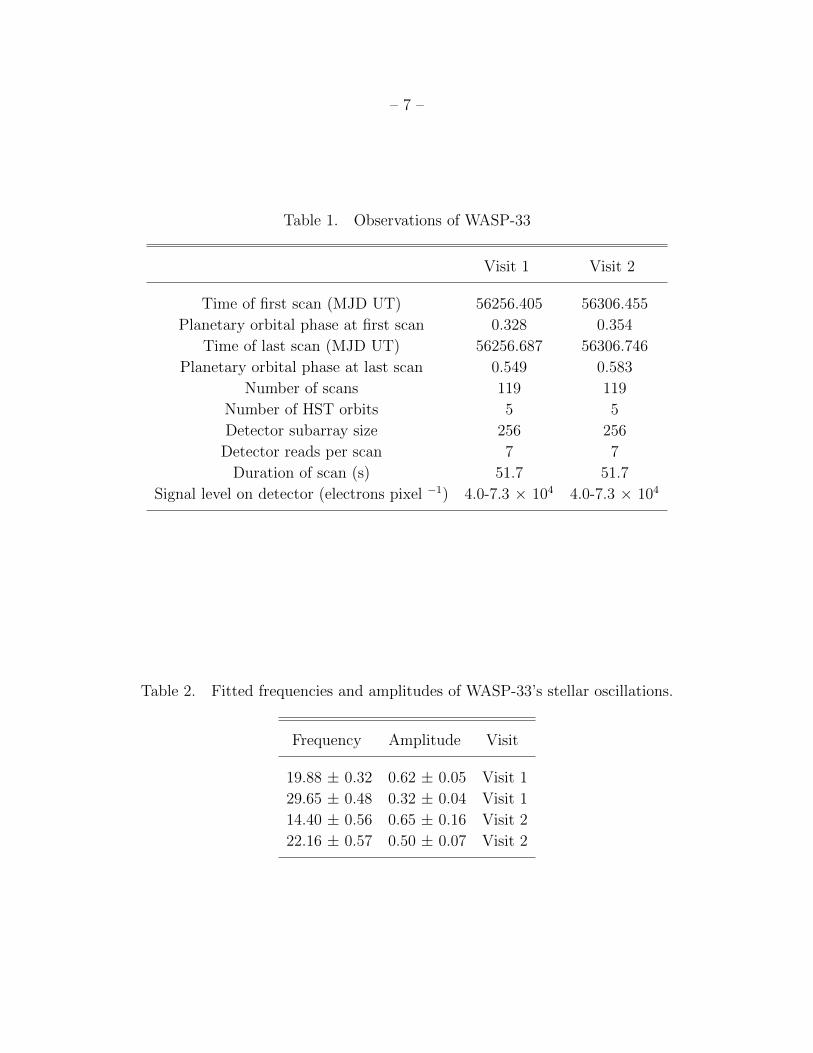
Table 1. Observations of WASP-33

Visit 1 Visit 2

Time of first scan (MJD UT) 56256.405 56306.455

Planetary orbital phase at first scan 0.328 0.354

Time of last scan (MJD UT) 56256.687 56306.746

Planetary orbital phase at last scan 0.549 0.583

Number of scans 119 119

Number of HST orbits 5 5

Detector subarray size 256 256

Detector reads per scan 7 7

Duration of scan (s) 51.7 51.7

Signal level on detector (electrons pixel −1) 4.0-7.3 × 104 4.0-7.3 × 104

Table 2. Fitted frequencies and amplitudes of WASP-33’s stellar oscillations.

Frequency Amplitude Visit

19.88 ± 0.32 0.62 ± 0.05 Visit 1

29.65 ± 0.48 0.32 ± 0.04 Visit 1

14.40 ± 0.56 0.65 ± 0.16 Visit 2

22.16 ± 0.57 0.50 ± 0.07 Visit 2

– 8 –

our relative wavelength-dependent eclipse depths since we subtract a scaled version of the

residual noise from each bin. Additionally, because the first orbit of WFC3 observations

tends to be more noisy than subsequent orbits (Mandell et al. 2013; Deming et al. 2012),

we do not include this orbit for the band-integrated fitting process (including fitting for the

stellar oscillations), though we do incorporate it later in our wavelength-dependent relative

analysis.

4.1.2. Nonlinearity Correction

WASP-33 is an early-type star, and the flux incident on the detector at the short-

est wavelength of the grism response is almost a factor of two larger than the flux at the

longest wavelength. Since we want to optimize the photon-limited SNR at even the longest

wavelength, we exposed the spectra to the highest possible fluence levels, reaching 7 × 104

electrons per pixel at the short wavelength end. Since this is comparable to the full well

value of the detector, we applied a correction for detector nonlinearity, as described in Sec.

6.5.1 of the WFC3 Data Handbook 2.1. We used coefficients valid for quadrant one of the

detector, extracted from the calibration files at STScI. Our calculated correction increases

the eclipse depths by 25 parts per million at our shortest wavelength, decreasing to about 6

parts per million at the longest wavelength we analyze. These corrections do not affect our

scientific conclusions, which would be virtually identical if we had omitted the non-linearity

correction.

4.1.3. Spectral Shifts With Time

In order to correct for possible variations in channel flux due to shifts across the peak

of spectral features with time, we calculated the shift in the horizontal/spectral direction

referenced to a template exposure from our data. We examined two main strategies for

measuring the magnitude of the shift with time. Our initial method was to measure the

spectrum at the steeply sloped edges of the grism response. Due to the steep slope, sensitivity

due to spectral shifting is greatest at these wavelengths; however, these wavelengths mostly

do not overlap with those used in our final analysis, which are located across the central,

flatter region of the grism response. If the shift of spectrum is identical at all wavelengths,

this should not impact the final results; however, as we describe below, this was not the case.

The alternative strategy is to use only those wavelengths also used for the subsequent light

curve analysis. We describe our analysis of both strategies in greater detail, along with their

results, below.

– 9 –

In our initial analysis procedure, which was adapted from the method used in Mandell

et al. (2013), we fit the slope of the pixels at the short-wavelength and long-wavelength edges

of the spectrum. At these wavelengths the sensitivity curve causes the shape of the spectrum

to change most dramatically, resulting in a high-precision measurement of the spectral shift

in each exposure. The slopes measured at both edges of the spectrum were averaged to

further decrease the effective uncertainty of the measurement for each exposure. We used

the zeroth-order coefficient of this fit to determine the shift of each spectrum relative to the

first exposure in the time series.

We compared this strategy to that employed by Deming et al. (2013), which used instead

the central region of the spectrum to measure the shifts. This region is flat compared to the

edges, but does contain modulation in the spectral response. In this method, we created a

template spectrum comprised of an average of the exposures in the time series immediately

preceding and following eclipse. We interpolated the template spectrum onto a wavelength

grid shifted in either direction up to a pixel and a half, stepping in 0.001 pixel increments,

and saved each shifted spectrum. For each exposure, we compared the observed spectrum

with each shifted template spectrum. We also allowed the template spectrum a linear stretch

in intensity. We calculated the rms for each comparison; the shift corresponding to the lowest

rms is saved as our best-fit spectral shift.

We compared the two spectral shift measurement strategies, finding that if the edges of

the spectrum are included for the latter method, then the resulting shifts match the “edge

only” measurements of our method very closely. If instead only the central region of the

spectrum is used to determine the shifts, the measured shifts result in significant change in

the final eclipse spectrum. This result indicates that the shape or placement of the grism

sensitivity function changes as a function of time or placement on the detector, possibly

due to changes in the optical path as part of the thermal breathing modes of the telescope.

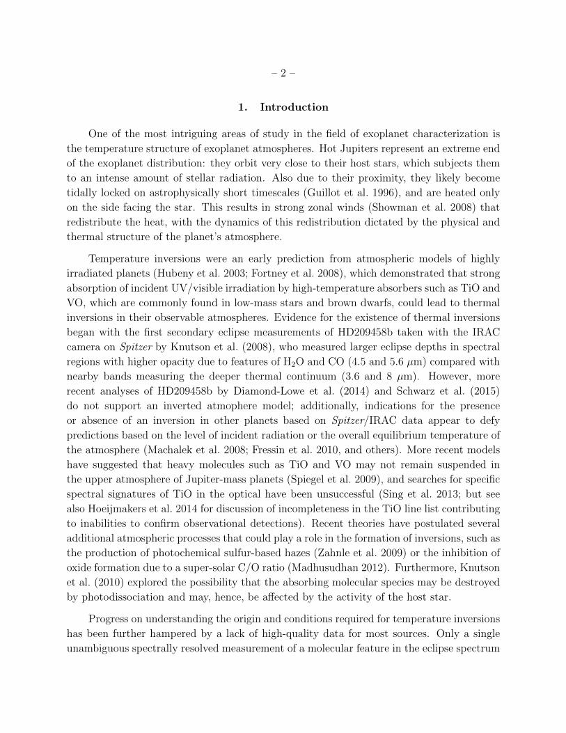
The horizontal shifts produced from the entire central region for the two visits are plotted

in Figure 1 for reference. The use of the “center-only” spectral shifts resulted in a lower

residual rms for the resulting light curves, indicating that the fit was improved by using

shifts derived from the same portion of the spectrum as the light curves themselves.

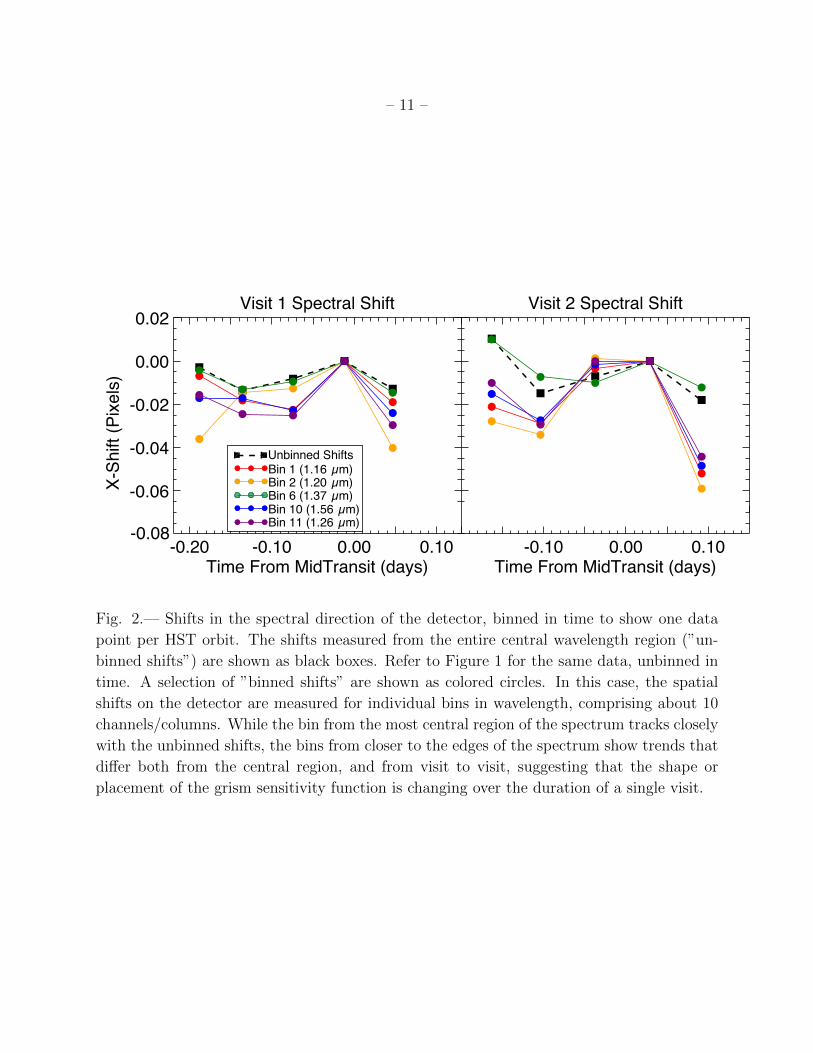
For consistency, we further extended this analysis by determining the specific spectral

shift for the specific portion of the spectrum associated with each binned light curve, and

using that set of shifts in the systematic decorrelation procedure. This has the advantage of

using the set of shifts that best describe the region of the spectrum used by each bin, since

the stellar intensity can vary greatly across the WFC3 grism response. However, the modest

wavelength range of the WFC3 grism and the minimal temperature variations expected due

to stellar oscillations ensure that our results show no spectral response to these pulsating

– 10 –

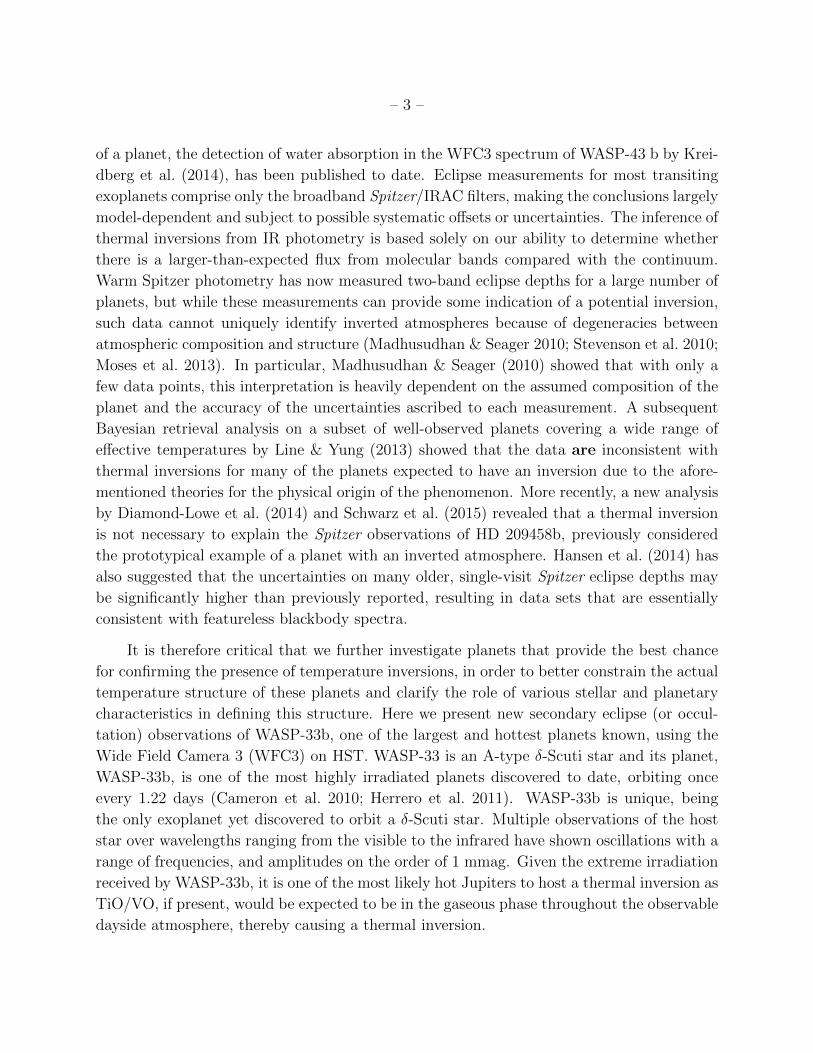
modes. As seen in Figure 2, the overall trend of the shifts with time does change with

wavelength, at least on a visit-long level; finer analysis is not possible due to the scatter

in the measurements. We found that using the bin-specific spectral shifts resulted in final

spectra for both visits that were consistent within uncertainties; on the contrary, using a

single shift value led to larger deviations between the visits, especially at short wavelengths.

Given this, we advocate careful inspection of the shift of the spectrum on the detector with

time, and for this work, we use these binned shifts for our final analysis.

In all cases, the shifts take the form of a repeating, inter-orbit pattern, as well as

a visit-long slope. We removed a visit-long linear trend from the xshifts, since a visit-

long trend in flux is also seen in previous WFC3 data sets and we choose to instead fit

for this slope as an independent parameter in our light curve fit. Alternatively, we also

examined the shift correction strategy from Deming et al. (2013), in which we interpolate

each exposure’s spectrum onto a shifted wavelength grid according to its best-measured shift

value (as determined by the rms) and use these shifted spectra for light curve fitting. In

this case, we do not use the scaled xshifts as a parameter in our MCMC fitting; instead, we

shift the spectra themselves. We find that the final derived spectrum is minimally affected

by the method of correction (interpolation vs xshift scaling), so long as the same wavelength

ranges (center, center + edges, or binned central region) are used to measure the shifts for

both methods.

Visit 2 Spectral Shift

−0.20 −0.10 0.00 0.10Time From MidTransit (days)

Visit 1 Spectral Shift

−0.20 −0.10 0.00Time From MidTransit (days)

−0.10

−0.05

0.00

0.05

0.10

X−Sh

ift (P

ixel

s)

Fig. 1.— Shifts in the spectral direction of the detector for both visits across the eclipse

duration. These shifts have been measured using the entire central region of the WFC3

wavelength coverage.

– 11 –

Visit 2 Spectral Shift

-0.10 0.00 0.10Time From MidTransit (days)

Visit 1 Spectral Shift

-0.20 -0.10 0.00 0.10Time From MidTransit (days)

-0.06

-0.04

-0.02

0.00

0.02

X-Sh

ift (P

ixel

s)

Unbinned ShiftsBin 1 (1.16 µm)Bin 2 (1.20 µm) Bin 6 (1.37 µm)

-0.08Bin 10 (1.56 µm)Bin 11 (1.26 µm)

Fig. 2.— Shifts in the spectral direction of the detector, binned in time to show one data

point per HST orbit. The shifts measured from the entire central wavelength region (”un-

binned shifts”) are shown as black boxes. Refer to Figure 1 for the same data, unbinned in

time. A selection of ”binned shifts” are shown as colored circles. In this case, the spatial

shifts on the detector are measured for individual bins in wavelength, comprising about 10

channels/columns. While the bin from the most central region of the spectrum tracks closely

with the unbinned shifts, the bins from closer to the edges of the spectrum show trends that

differ both from the central region, and from visit to visit, suggesting that the shape or

placement of the grism sensitivity function is changing over the duration of a single visit.

– 12 –

4.2. Band-Integrated Eclipse Curve Fitting

We fit a band-integrated eclipse curve first, in order to determine best-fit values for those

parameters that are not wavelength dependent (as in the case for the stellar oscillations),

and in order to use the residuals of this band-integrated fit as a component in our analysis

of spectral channels or bins (see Mandell et al. (2013) for further explanation and details of

our fitting process). For both band-integrated and spectral channels/bins, we use a Markov

Chain Monte Carlo (MCMC) routine to determine our best-fit parameters. We locked all

orbital parameters, leaving open for fitting only the eclipse depth, slope, and sine terms.

Orbital parameters are listed in Table 3.

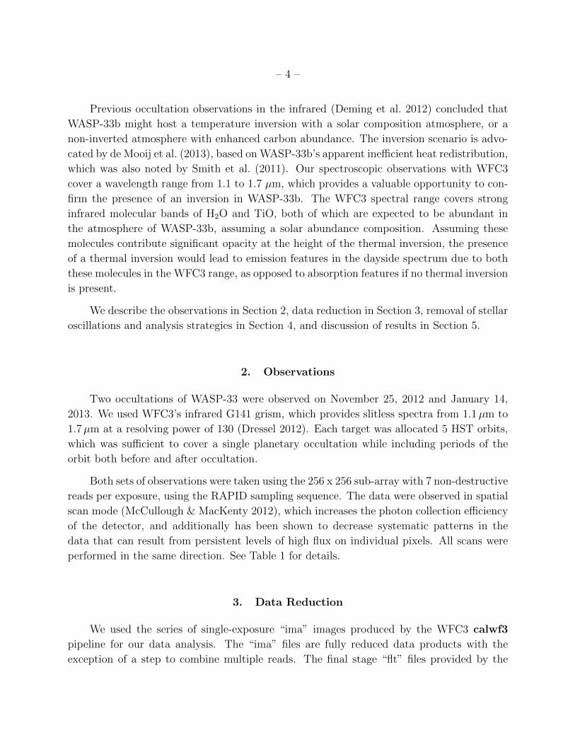
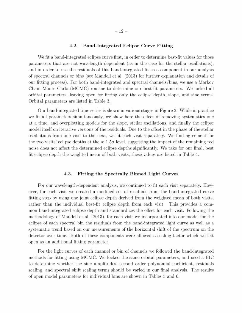
Our band-integrated time series is shown in various stages in Figure 3. While in practice

we fit all parameters simultaneously, we show here the effect of removing systematics one

at a time, and overplotting models for the slope, stellar oscillations, and finally the eclipse

model itself on iterative versions of the residuals. Due to the offset in the phase of the stellar

oscillations from one visit to the next, we fit each visit separately. We find agreement for

the two visits’ eclipse depths at the ≈ 1.5σ level, suggesting the impact of the remaining red

noise does not affect the determined eclipse depths significantly. We take for our final, best

fit eclipse depth the weighted mean of both visits; these values are listed in Table 4.

4.3. Fitting the Spectrally Binned Light Curves

For our wavelength-dependent analysis, we continued to fit each visit separately. How-

ever, for each visit we created a modified set of residuals from the band-integrated curve

fitting step by using one joint eclipse depth derived from the weighted mean of both visits,

rather than the individual best-fit eclipse depth from each visit. This provides a com-

mon band-integrated eclipse depth and standardizes the offset for each visit. Following the

methodology of Mandell et al. (2013), for each visit we incorporated into our model for the

eclipse of each spectral bin the residuals from the band-integrated light curve as well as a

systematic trend based on our measurements of the horizontal shift of the spectrum on the

detector over time. Both of these components were allowed a scaling factor which we left

open as an additional fitting parameter.

For the light curves of each channel or bin of channels we followed the band-integrated

methods for fitting using MCMC. We locked the same orbital parameters, and used a BIC

to determine whether the sine amplitudes, second order polynomial coefficient, residuals

scaling, and spectral shift scaling terms should be varied in our final analysis. The results

of open model parameters for individual bins are shown in Tables 5 and 6.

– 13 –

Table 3. Orbital and Stellar Parameters for WASP-33 a

Parameter Value

Period (days) 1.2198709

i (◦) 86.2 ± 0.2

Rp/R∗ 0.1143 ± 0.0002

a/R∗ 3.69 ± 0.01

Semi-major axis (AU) 0.0259 +0.0002−0.0005

e 0.00 ± 0.00

M∗ (M�) 1.561+0.045−0.079

Spectral type A5

H band Magnitude 7.5

[Fe/H] 0.1 ± 0.2 c

aValues from Kovacs et al. (2013) except

where otherwise noted.

cFrom Cameron et al. (2010).

Table 4. Band Integrated Results

Visit Eclipse Depth (%)

Visit 1 0.129 ± 0.009

Visit 2 0.110 ± 0.010

Combined 0.119 ± 0.006

– 14 –

WASP-33 Visit 1 White Light

0.9960.9970.9980.9991.0001.0011.0021.003

Nor

mal

ized

Flu

x

0.997

0.998

0.999

1.000

1.001

Slop

e C

orre

cted

0.997

0.998

0.999

1.000

1.001

Sine

Cor

rect

ed

-0.20 -0.15 -0.10 -0.05 0.00 0.05 0.10Time From Mid-Transit (days)

-0.0015-0.0010-0.00050.00000.00050.00100.0015

Fina

l Tra

nsit

Res

idua

ls

WASP-33 Visit 2 White Light

0.9970.9980.9991.0001.0011.0021.003

Nor

mal

ized

Flu

x

0.998

0.999

1.000

1.001

Slop

e C

orre

cted

0.997

0.998

0.999

1.000

1.001

Sine

Cor

rect

ed

-0.15 -0.10 -0.05 0.00 0.05 0.10 0.15Time From Mid-Transit (days)

-0.0015-0.0010-0.00050.00000.00050.00100.0015

Fina

l Tra

nsit

Res

idua

ls

Fig. 3.— Band-integrated light curves for both visits in black with various model fits in red.

From top to bottom, the plots show a) the normalized data with a model for the visit-long

slope effect; b) the slope corrected data with a model for the stellar oscillations; c) the slope

and oscillation corrected data with a model for the eclipse; d) the residuals for the full fit.

Parameters are fit concurrently in MCMC, and are shown here in stages for clarification on

the relative contributions of each parameter.

– 15 –

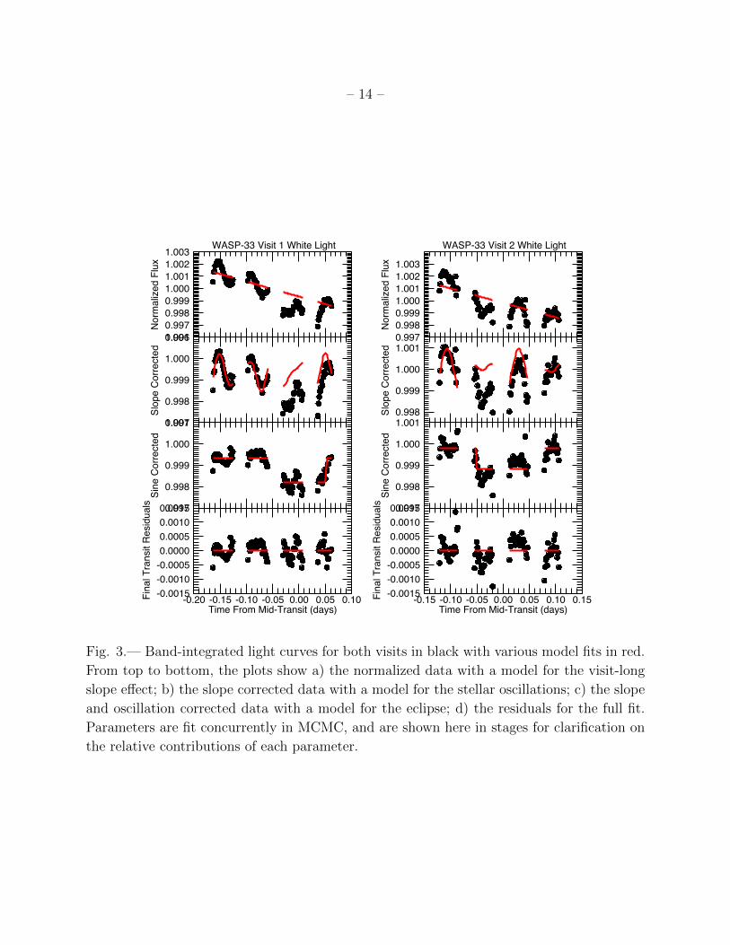
Table 5. Visit 1: Open parameters for each bin as determined by BIC. For each binned

light curve, we test the significance of additional parameters with a BIC. Parameters

determined to significantly improve the fit are marked with a checkmark. We also tested a

residuals scaling coefficient, but found that it was not significant for any bin, and so we do

not include the null result in our table.

Wavelength Eclipse Out of Linear Sine XShifts 2nd Order

(µm) Depth Eclipse Flux Slope Amplitudes Scaling Coeffecient

1.16 X X X X X1.20 X X X X X1.24 X X X X X1.28 X X X X1.32 X X X X1.37 X X X X1.41 X X X X X1.46 X X X X X1.51 X X X X X1.56 X X X X X1.61 X X X X X

Table 6. Visit 2: Open parameters for each bin as determined by BIC. For each binned

light curve, we test the significance of additional parameters with a BIC. Parameters

determined to significantly improve the fit are marked with a checkmark. We also tested a

residuals scaling coefficient and a second order polynomial term, but found that they were

not significant for any bins, and so we do not include the null results in our table.

Wavelength Eclipse Out of Linear Sine XShifts

(µm) Depth Eclipse Flux Slope Amplitudes Scaling

1.16 X X X X1.20 X X X X1.24 X X X X1.28 X X X X X1.32 X X X X1.37 X X X X1.41 X X X X X1.46 X X X X1.51 X X X X1.56 X X X X1.61 X X X X

– 16 –

In general we find that the same terms make significant contributions for all the bins in

a single visit. The light curves are typically fit best by a model including a linear slope term,

unscaled band-integrated residuals and sine amplitudes, and a scaled version of the spectral

shifts. A fit for a second-order polynomial term for the visit-long trend (as suggested by

Stevenson et al. 2014) passed the BIC for most bins in Visit 1, but did not pass for any bins

in Visit 2. In all cases we chose the open parameters based on the BIC, on a bin-by-bin

basis.

0.0000

0.0005

0.0010

0.0015

0.0020

0.0025

Eclip

se D

epth

1.1 1.2 1.3 1.4 1.5 1.6 1.7Wavelength (μm)

0.0007

0.0008

0.0009

0.0010

0.0011

0.0012

0.0013

0.0014

Eclip

se D

epth

Blackbody CurveVisit 1Visit 2Combined

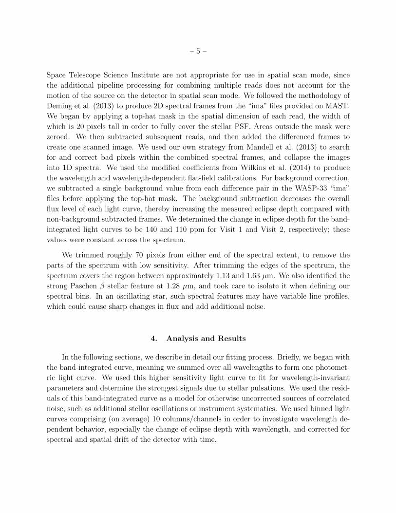
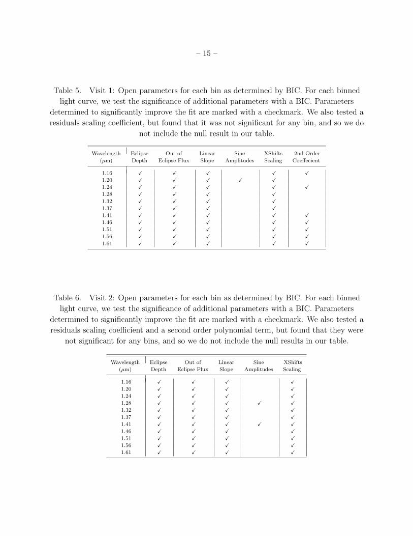
Fig. 4.— Top: Unbinned spectrum. Here, every detector column was assigned a wavelength,

a light curve was extracted, and the eclipse depth measured. Bottom: Binned spectrum. In

this case, multiple detector columns (ten columns, on average) were combined to make one

light curve, and the eclipse depth measured. Points are plotted at the mean wavelength for

each bin. For both plots, Visit 1 is in red, Visit 2 in blue, and the combined visits are in

black. Combined visits use a weighted mean. The largest discrepancies between visits are

seen near the stellar hydrogen line at 1.28 µm. Blackbody curve is shown as a dashed line,

with the best-fit planetary temperature of 2950 K.

Finally, we used an uncertainty-weighted mean to combine both visits in our final stage

– 17 –

of analysis, and these results are presented in Figure 4 and in Tables 7 (for the channels)

and 8 (for the bins). The results from both visits agree to within the 1-σ uncertainties for

almost all of the spectral bins, with the only major discrepancies appearing for two bins

near the stellar hydrogen line at 1.28 µm. This difference between visits for the hydrogen

feature is most likely due to variability in the depth of the stellar hydrogen line, which can

oscillate differently than the overall stellar continuum; we therefore consider this offset to be

uncorrectable without simultaneous measurements of other hydrogen spectral features.

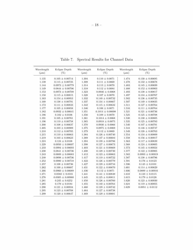
– 18 –

Table 7. Spectral Results for Channel Data

Wavelength Eclipse Depth Wavelength Eclipse Depth Wavelength Eclipse Depth

(µm) (%) (µm) (%) (µm) (%)

1.135 0.105 ± 0.00714 1.304 0.110 ± 0.0071 1.474 0.130 ± 0.00695

1.139 0.115 ± 0.00725 1.309 0.111 ± 0.0069 1.478 0.132 ± 0.00678

1.144 0.0973 ± 0.00779 1.314 0.113 ± 0.0070 1.483 0.145 ± 0.00699

1.149 0.0844 ± 0.00706 1.318 0.112 ± 0.0084 1.488 0.152 ± 0.00903

1.153 0.0973 ± 0.00709 1.323 0.0946 ± 0.0068 1.493 0.138 ± 0.00817

1.158 0.115 ± 0.00815 1.328 0.107 ± 0.0070 1.497 0.134 ± 0.00767

1.163 0.154 ± 0.00953 1.332 0.140 ± 0.00732 1.502 0.136 ± 0.00735

1.168 0.138 ± 0.00791 1.337 0.134 ± 0.00667 1.507 0.149 ± 0.00835

1.172 0.111 ± 0.00833 1.342 0.115 ± 0.00632 1.511 0.127 ± 0.00764

1.177 0.105 ± 0.00858 1.346 0.106 ± 0.0071 1.516 0.111 ± 0.00764

1.182 0.0932 ± 0.00641 1.351 0.1014 ± 0.00698 1.521 0.121 ± 0.00736

1.186 0.102 ± 0.0106 1.356 0.109 ± 0.0070 1.525 0.125 ± 0.00708

1.191 0.105 ± 0.00761 1.361 0.1014 ± 0.0068 1.530 0.130 ± 0.00805

1.196 0.119 ± 0.00758 1.365 0.0918 ± 0.0075 1.535 0.125 ± 0.00783

1.200 0.108 ± 0.00637 1.370 0.0930 ± 0.0066 1.540 0.107 ± 0.00791

1.205 0.103 ± 0.00909 1.375 0.0975 ± 0.0069 1.544 0.146 ± 0.00747

1.210 0.112 ± 0.00705 1.379 0.112 ± 0.0069 1.549 0.128 ± 0.00763

1.215 0.110 ± 0.00663 1.384 0.126 ± 0.00740 1.554 0.134 ± 0.00809

1.219 0.103 ± 0.00623 1.389 0.137 ± 0.00683 1.558 0.156 ± 0.00917

1.224 0.124 ± 0.0108 1.394 0.139 ± 0.00786 1.563 0.117 ± 0.00839

1.229 0.0950 ± 0.00697 1.398 0.127 ± 0.00673 1.568 0.124 ± 0.00805

1.233 0.0994 ± 0.00693 1.403 0.121 ± 0.00669 1.573 0.145 ± 0.00924

1.238 0.0841 ± 0.00736 1.408 0.129 ± 0.00730 1.577 0.122 ± 0.00905

1.243 0.0889 ± 0.00683 1.412 0.123 ± 0.00663 1.582 0.0993 ± 0.00919

1.248 0.0898 ± 0.00736 1.417 0.119 ± 0.00722 1.587 0.138 ± 0.00796

1.252 0.0980 ± 0.00718 1.422 0.126 ± 0.00779 1.591 0.176 ± 0.0123

1.257 0.108 ± 0.00736 1.427 0.129 ± 0.00716 1.596 0.145 ± 0.0101

1.262 0.100 ± 0.00687 1.431 0.122 ± 0.00670 1.601 0.114 ± 0.00829

1.266 0.0960 ± 0.00689 1.436 0.112 ± 0.0071 1.606 0.0889 ± 0.00916

1.271 0.0582 ± 0.0101 1.441 0.141 ± 0.00849 1.610 0.123 ± 0.0115

1.276 0.0305 ± 0.00960 1.445 0.125 ± 0.00811 1.615 0.179 ± 0.0128

1.281 0.245 ± 0.0252 1.450 0.126 ± 0.00760 1.620 0.123 ± 0.00930

1.285 0.179 ± 0.0184 1.455 0.140 ± 0.00764 1.624 0.119 ± 0.00955

1.290 0.121 ± 0.00934 1.460 0.129 ± 0.00742 1.629 0.0951 ± 0.0112

1.295 0.123 ± 0.00708 1.464 0.127 ± 0.00738

1.299 0.120 ± 0.00647 1.469 0.129 ± 0.00681

– 19 –

4.4. Error Analysis

Our measured uncertainties were initially drawn from the MCMC posterior probability

distributions. In order to estimate the impact of our red noise, we used a modified version of

the residuals permutation method (Gillon et al. 2007), which involves shifting (permutating)

the time series of the residual noise via the “prayer-bead” method. In addition to shifting

the residual noise series left over from subtracting the light-curve model, we also inverted our

residuals (multiplying by -1) and reversed both the inverted and non-inverted residuals in

time to produce four different sets of residual noise. This yields 4 × N permutations, where

N is the number of exposures. We deemed this extra step useful because of the otherwise

limited number of possible permutations, which did not yield clear results from a traditional

residuals permutation analysis. For each channel or bin of channels, we use whichever is

higher, the uncertainty from MCMC or residuals permutation. For Visit 1, we find that

uncertainties from residuals permutation are on average 1.47 times higher than uncertainties

from MCMC, while for Visit 2 uncertainties from residuals permutation are 1.20 times higher.

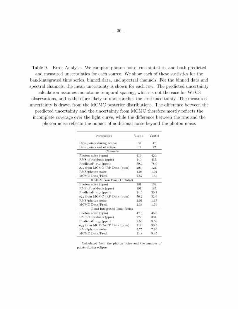
We compared the photon noise to the rms of our white light, channel, and binned

data.We present our results in Table 9. In general we find that a substantial amount of

red noise remains in our band integrated light curves after removal of our best fit models.

However, the temporal morphology of the red noise does not change with wavelength, and

by subtracting our band-integrated residuals from each bin we are able to closely approach

the photon noise limit for our channels and bins. For our channels and bins, we find an rms

∼1.05 times the photon noise.

We also compare the measured MCMC + residuals permutation uncertainty to a pre-

dicted eclipse depth uncertainty. This prediction is based on the photon noise (or rms) and

the number of exposures in eclipse versus out of eclipse. The predicted uncertainty calcu-

lation assumes monotonic temporal spacing, which is not the case for WFC3 observations.

We find that our measured eclipse depth uncertainties for the channels and bins are between

∼1.5-2.5 times the predicted uncertainty, and we ascribe this to the contributions from the

uneven sampling of HST orbits and the residual red noise in the light curves. In previous

studies we found that the lack of complete and evenly spaced temporal coverage during the

eclipse is likely the cause of this failure to meet the predicted uncertainty, even for photon-

limited results. In this same comparison of measured versus predicted uncertainties, we note

that Visit 1 is further from the predicted uncertainty than Visit 2. Visit 1 has substantially

fewer points post-eclipse than Visit 2, which can be detrimental to the uncertainty on eclipse

fitting. Additionally, Visit 1 has a higher rate of spectral drift; while we perform corrections

for this drift, it remains an additional source of uncertainty. Given these factors, we feel

confident that the uncertainty we measure accurately reflects the sources of uncertainty in

– 20 –

the data.

5. Discussion

The hot Jupiter WASP-33b is one of the most irradiated hot Jupiters known and hence

is among the most favorable candidates to host a thermal inversion in its dayside atmosphere.

Studies in the past have suggested that extremely irradiated hot Jupiters should host ther-

mal inversions due to strong absorption of incident stellar light by absorbers such as TiO

and VO (Hubeny et al. 2003; Fortney et al. 2008). While Spiegel et al. (2009) have suggested

that TiO and VO may not remain aloft in some hot Jupiter atmospheres due to downward

drag by gravitational settling and condensation overtaking upward vertical mixing, the ex-

treme irradiation of WASP-33b should maintain atmospheric temperatures above the TiO

condensation point at all altitudes. However, alternate theories regarding the presence of

thermal inversions do not depend solely on temperature. Madhusudhan et al. (2011) and

Madhusudhan (2012) suggested that high C/O ratios could also deplete inversion-causing

compounds such as TiO and VO in hot Jupiters, thereby precluding the formation of thermal

inversions, and Knutson et al. (2010) proposed that the formation of inversions may instead

be correlated with chromospheric activity, implying that hot Jupiters orbiting active stars

are less likely to host thermal inversions (though their study did not include A-stars such as

WASP-33). While the existence of an inversion has been questioned in the archetype planet

HD 209458b (Diamond-Lowe et al. 2014; Schwarz et al. 2015), it is nevertheless reasonable

to hypothesize that strong stellar irradiation may cause substantial perturbations in the

temperature structure of hot Jupiter atmospheres. Given its extreme atmospheric condi-

tions and bright thermal emission, WASP-33b presents a valuable opportunity to constrain

the various hypotheses regarding thermal inversions in hot Jupiters, but previously reported

photometric observations from Spitzer and ground-based facilities have been unable to con-

clusively constrain the presence of an inversion (Deming et al. 2012; de Mooij et al. 2013).

With the inclusion of our spectrum from the WFC3 instrument on HST, we can significantly

improve these constraints.

5.1. Atmospheric Models and Parameter Retrieval

We modeled the temperature and composition of the planet’s atmosphere and retrieved

its properties using the retrieval technique of Madhusudhan et al. (2011) and Madhusudhan

(2012). The model computes line-by-line radiative transfer for a plane-parallel atmosphere

with the assumptions of hydrostatic equilibrium and global energy balance, as described in

– 21 –

1.2

1.0

0.8

0.61.2 1.3 1.4 1.5 1.6

WASP-33b

Inversion

No Inversion

Isothermal

F plan

et /

F star

(10-3

)

λ (μm)1 105

8

6

4

2

2 3 4

WFC3 Data

No Inv. Inv.

Isoth.

ThermalPro�le

10-4

10-3

10-2

10-1

100

101

102

10-5

P (bar)

2.0 3.0 4.01.0T (1000K)

Data (HST, Spitzer and Ground)

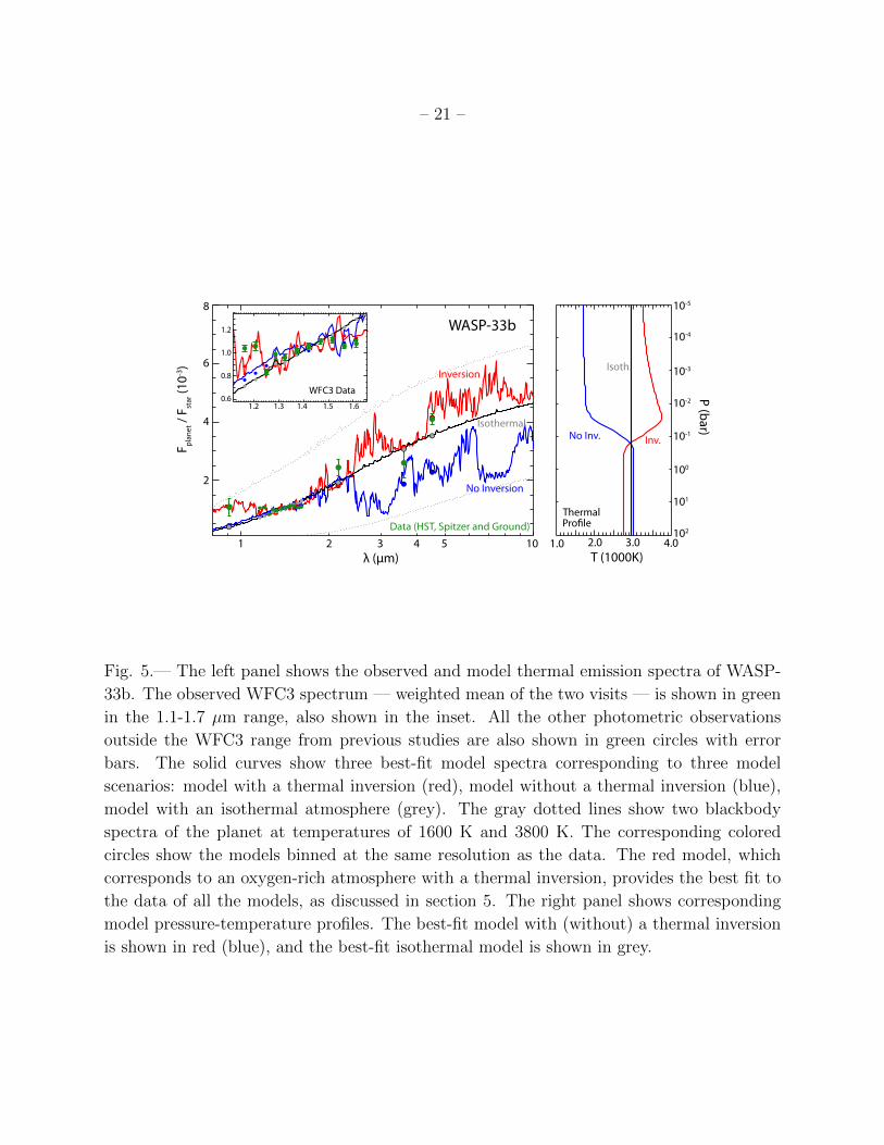
Fig. 5.— The left panel shows the observed and model thermal emission spectra of WASP-

33b. The observed WFC3 spectrum — weighted mean of the two visits — is shown in green

in the 1.1-1.7 µm range, also shown in the inset. All the other photometric observations

outside the WFC3 range from previous studies are also shown in green circles with error

bars. The solid curves show three best-fit model spectra corresponding to three model

scenarios: model with a thermal inversion (red), model without a thermal inversion (blue),

model with an isothermal atmosphere (grey). The gray dotted lines show two blackbody

spectra of the planet at temperatures of 1600 K and 3800 K. The corresponding colored

circles show the models binned at the same resolution as the data. The red model, which

corresponds to an oxygen-rich atmosphere with a thermal inversion, provides the best fit to

the data of all the models, as discussed in section 5. The right panel shows corresponding

model pressure-temperature profiles. The best-fit model with (without) a thermal inversion

is shown in red (blue), and the best-fit isothermal model is shown in grey.

– 22 –

Madhusudhan & Seager (2009). The composition and pressure-temperature (P -T ) profile

of the dayside atmosphere are free parameters in the model. The model includes all the

major opacity sources expected in hot Jupiter atmospheres, namely H2O, CO, CH4, CO2,

C2H2, HCN, TiO, VO, and collision-induced absorption (CIA) due to H2-H2, as described

in Madhusudhan (2012). Our molecular line lists are obtained from Freedman et al. (2008),

Freedman (personal communication, 2009), Rothman (2005), Karkoschka & Tomasko (2010),

and Karkoschka (personal communication, 2011). Our CIA opacities are obtained from

Borysow et al. (1997) and Borysow (2002). A Kurucz model Castelli & Kurucz (2004) is

used for the stellar spectrum, and the stellar and planetary parameters are adopted from

Cameron et al. (2010).

We used our WFC3 observations together with previously published photometric data

(Deming et al. 2012; de Mooij et al. 2013; Smith et al. 2011) to obtain joint constraints on

the chemical composition and temperature structure of the planet. We explored the model

parameter space using a Markov Chain Monte Carlo algorithm (Madhusudhan et al. 2011)

and determined regions of model space that best explain the data. Our model space includes

models with and without thermal inversions, and models with oxygen-rich as well as carbon-

rich compositions. To accommodate the uncertainty in the overall band offset resulting from

our separate fits to the band-integrated light curve and each individual bin, we allowed a

constant offset on the WFC3 spectrum as a free parameter in our model fits, with a prior

constraint on the explored range based on the derived band-integrated uncertainty. Thus,

the model has twelve free parameters: five for the P -T profile, six for uniform mixing ratios of

six molecules (H2O, CO, CH4, CO2, C2H2, HCN), and one parameter for the WFC3 offset.

For the inversion models we set the TiO and VO abundances to their solar abundance

composition, whereas for the non-inversion model we assume TiO and VO are not present

in significant quantities. We ran separate model fits to the data assuming inverted and non-

inverted temperature profiles. We also investigated fits with isothermal temperature profiles

which result in featureless black body spectra; such a model has only two free parameters,

the isothermal temperature and the WFC3 offset.

We find that the sum-total of observations are best explained by a dayside atmosphere

with a temperature inversion and an oxygen-rich composition with a slightly sub-solar abun-

dance of H2O (see Figure 5). Previous photometric observations were consistent with two

distinct models (Deming et al. 2012): (a) a model with oxygen-rich composition with a

strong thermal inversion, and (b) a model with a carbon-rich composition but with no ther-

mal inversion. In our current work, we use our WFC3 observations to break the degeneracies

between these models, constrain the abundance of H2O, and provide strong evidence for a

temperature inversion caused by TiO. Figure 5 shows the observed spectrum along with

three best-fit model spectra in three model categories, one with a thermal inversion, one

– 23 –

without a thermal inversion, and another with an isothermal profile. The corresponding

pressure-temperature profiles are also shown. The best-fit inverted model has a χ2 of 98, the

best-fit non-inverted model has a χ2 of 243, and the best-fit blackbody (BB) spectrum has

a χ2 of 351. The causes of the remaining differences between the best-fit thermally-inverted

atmosphere model and the WFC3 data points are unclear at this point, but the relative

quality of fit between the three models can still be assessed robustly using the Bayesian

Information Criterion (BIC) given by BIC= χ2 + k ln(N), where k is the number of free

parameters and N is the number of data points (15). The BIC for the three best-fit models

described above are 130.5 for the inverted model, 275.5 for the non-inverted model, and 356.4

for the blackbody model, implying that the inverted model provides a significantly better fit

to all the data and that the spectrum is not a blackbody.

We note that for each model category a population of ‘best-fit’ models are found with

similar χ2 values. Here we choose the most physically and chemically plausible model for

each category by determining the most likely combinations of molecular mixing ratios in

these solutions for the corresponding temperatures assuming equilibrium or non-equilibrium

chemistry (Madhusudhan 2012; Moses et al. 2013). For example, the criteria used for O-rich

models are that (a) CO must be comparable to the well-constrained H2O abundance, (b)

CH4,C2H2, and HCN are below 10−5, and (c) CO2 is below 10−6. The best-fit inversion

model has an O-rich composition with emission features due to CO, TiO, and H2O. The

mixing ratios of CO and H2O in the best-fit model are marginally sub-solar at ∼10−4 each,

whereas TiO and all the other molecules (e.g. CH4, C2H2, HCN) have nearly solar mixing

ratios; i.e. consistent with mixing ratios predicted by chemical equilibrium assuming solar

elemental abundances. The model fit to the 4.5 µm IRAC data point is due to the strong CO

emission feature, whereas the TiO emission feature is responsible for the fit in the z′ band

(at 0.9 µm) and the bluer half of our WFC3 data. Low-amplitude H2O emission features

provide reasonable fits to the remaining data in the WFC3 bandpass, whereas the continuum

emission is set by the temperature in the lower atmosphere of the inverted temperature profile

shown in Figure 5. On the contrary, the non-inversion model fit shown in Figure 5 has a

C-rich composition, as discussed below, consistent with the findings of Deming et al. (2013),

and has a significantly poorer fit compared to the O-rich inversion model as discussed above.

While the non-inversion model provides a very good fit to most of the WFC3 data, it provides

a significantly poor fit to the two bluest WFC3 data points, the z′ point, and the 4.5 µm

IRAC point.

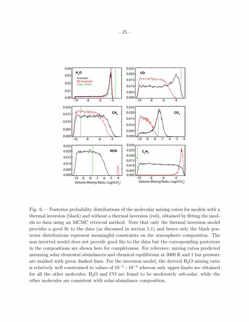
Figure 6 shows the posterior probability distributions of the chemical compositions for

each model, inverted versus non-inverted. Note that even though the non-inverted model

provides much worse fits to the data than the inverted model, we show the posterior distri-

butions on compositions for both models for completeness. The posteriors for the inverted

– 24 –

model are consistent with an O-rich atmosphere, albeit of marginally sub-solar metallicity.

The H2O abundance is well constrained to between 10−5 - 10−4, thanks to the WFC3 band-

pass which overlaps with a strong H2O band, whereas only upper-limits are obtained for all

the other molecules. The CO and H2O abundances are marginally sub-solar, but the upper-

limits on all the remaining molecules are consistent with a solar-type O-rich abundance

pattern. On the other hand, the posteriors for the non-inverted model similarly constrain

the H2O abundance but also require high abundances of HCN and C2H2 which are possible

only if the atmosphere is carbon-rich (i.e. C/O ≥ 1; Madhusudhan 2012; Kopparapu et al.

2013; Moses et al. 2013). However, these non-inverted models provide much worse fits to

the data compared to the inverted models, as discussed above, and hence the corresponding

constraints on the compositions are irrelevant. Nevertheless, these results still demonstrate

that it is in principle possible to detect C-rich atmospheres using a combination of WFC3

and Spitzer data.

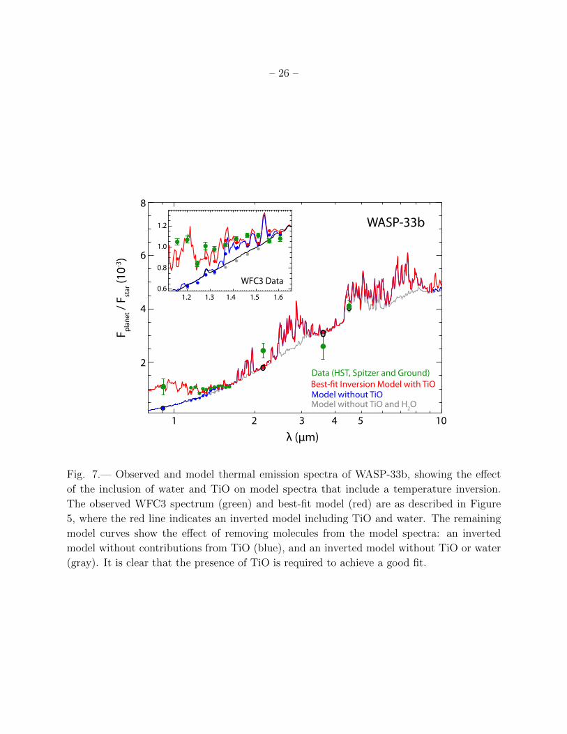
The inversion model fit supports not just evidence for a temperature inversion, but also

argues that the temperature inversion is due to TiO. Figure 7 shows the observed spectrum

along with three model spectra, all including a thermal inversion: one is our best-fit model

including both TiO and water, one lacks TiO, and the third lacks both TiO and water. It

is clear that not only a temperature inversion, but also the presence of TiO (and water) is

required in order to achieve a truly good fit to the observed data. As shown in previous

studies (Hubeny et al. 2003; Fortney et al. 2008), strong absorption of incident light due

to the strong UV/visible opacity of TiO can cause thermal inversions in hot Jupiters. On

the other hand, the infrared opacity of TiO contributes to the emission features of TiO in

the emergent spectrum of the planet similar to the emission features of other molecules in

the planetary atmosphere caused by a thermal inversion. Thus the simultaneous inference

of a thermal inversion and the presence of TiO presents a self-consistent case in favor of the

results. Our inference of TiO supports previous theoretical predictions that TiO should be

abundant in the hottest of oxygen-rich hot Jupiters, due to the lack of an effective vertical

or day-night cold trap (Perez-Becker & Showman 2013; Parmentier et al. 2013). However,

previous searches for TiO in other hot Jupiters using transmission spectroscopy have yielded

either secure non-detections (Huitson et al. 2013; Sing et al. 2013) or inconclusive results

(Desert et al. 2008). Two of these planets (HD 209458b and WASP-19b) are significantly

cooler than WASP-33b, but the lack of TiO absorption in the transmission spectrum of

WASP-12b (Teq ∼ 2500) may instead be due to either a high-altitude haze layer obscuring

any molecular absorption (Sing et al. 2013) or a chemical composition that is carbon-rich

rather than oxygen-rich (Madhusudhan et al. 2011; Stevenson et al. 2014).

However, since we cannot resolve individual spectral bands or lines of TiO in our spec-

trum, the evidence for TiO emission towards the blue end of WFC3 and in the z′ band is

– 25 –

0.04

0.03

0.02

0.01

0.00

0.020

0.005

0.010

0.015

0.000

0.0250.020

0.015

0.010

0.0050.000

0.020

0.0050.0100.015

0.000

0.0250.020

0.015

0.010

0.0050.000

0.0250.020

0.015

0.010

0.0050.000

Volume Mixing Ratio, Log(X/H2)-10 -9 -8 -7 -6 -10 -8 -6 -4

Volume Mixing Ratio, Log(X/H2)

-10 -8 -6 -4

-10 -8 -6 -4

-10 -9 -8 -7 -6 -5 -4

H2O CO

CH4 CO2

C2H2HCN

-10 -8 -6 -4

-5 -4

0.0250.030

InversionNo InversionSolar, 3000K

Fig. 6.— Posterior probability distributions of the molecular mixing ratios for models with a

thermal inversion (black) and without a thermal inversion (red), obtained by fitting the mod-

els to data using an MCMC retrieval method. Note that only the thermal inversion model

provides a good fit to the data (as discussed in section 5.1) and hence only the black pos-

terior distributions represent meaningful constraints on the atmospheric composition. The

non-inverted model does not provide good fits to the data but the corresponding posteriors

in the compositions are shown here for completeness. For reference, mixing ratios predicted

assuming solar elemental abundances and chemical equilibrium at 3000 K and 1 bar pressure

are marked with green dashed lines. For the inversion model, the derived H2O mixing ratio

is relatively well constrained to values of 10−5 - 10−4 whereas only upper-limits are obtained

for all the other molecules; H2O and CO are found to be moderately sub-solar, while the

other molecules are consistent with solar-abundance composition.

– 26 –

F plan

et /

F star

(10-3

)

λ (μm)1 105

8

6

4

2

2 3 4

1.2

1.0

0.8

0.61.2 1.3 1.4 1.5 1.6

WASP-33b

Best-�t Inversion Model with TiO

Model without TiO and H2O

WFC3 Data

Model without TiO

Data (HST, Spitzer and Ground)

Fig. 7.— Observed and model thermal emission spectra of WASP-33b, showing the effect

of the inclusion of water and TiO on model spectra that include a temperature inversion.

The observed WFC3 spectrum (green) and best-fit model (red) are as described in Figure

5, where the red line indicates an inverted model including TiO and water. The remaining

model curves show the effect of removing molecules from the model spectra: an inverted

model without contributions from TiO (blue), and an inverted model without TiO or water

(gray). It is clear that the presence of TiO is required to achieve a good fit.

– 27 –

not conclusive. Ostensibly, the presence of hazes/clouds in the atmosphere could lead to sig-

nificant particulate scattering at short wavelengths, as the scattering cross-sections typically

scale as an inverse-power-law of the wavelength (e.g. Evans et al. 2013; Sing et al. 2013).

However, such an interpretation is met with several challenges. Firstly, the blue-ward flux

would need to start rising abruptly below ∼1.25 µm, following a 20% increase in reflected

light over a 0.05µm spectral bin, which is inconsistent with the typical power law slope ex-

pected for the scattered light spectrum. Secondly, the planet orbits an A star (T ∼ 7400

K) for which the spectrum peaks at relatively short wavelengths (0.43 µm). Consequently,

the dominant contribution of the reflected light would be expected to be in the far blue

with significantly less contribution in the near-infrared which is where the current data need

strong flux. Therefore the contribution from emission by TiO represents the most plausible

explanation for the rise in the data at short wavelengths, but this inference can be further

verified by future observations using existing facilities. TiO has strong spectral features in

the red optical and near-infrared, between ∼0.7-1.1 µm as shown in Figure 7 (also see e.g.

Fortney et al. 2008; Madhusudhan 2012). Several existing instruments can enable observa-

tions in this bandpass, including HST WFC3 G102 grism spectroscopy in the ∼ 0.8-1.15 µm

range (Sing et al. 2014), and ground-based spectroscopy and/or photometry in the ∼0.7-1.2

µm range (e.g. Bean et al. 2011; Fohring et al. 2013; Chen et al. 2014).

Finally, we note that previous studies, both theoretical and observational, have sug-

gested that the hottest exoplanets may be the most inefficient at redistributing heat to their

night sides (Cowan & Agol 2011; Perez-Becker & Showman 2013). Our results are consistent

with those findings; if we compare the incoming radiation from the star with the outgo-

ing day-side flux from our best-fit inverted model, we derive a low day-night redistribution

(. 15%), as would be expected for a planet with day-side temperatures above 2200K. In

contrast, the best-fit non-inverted model, which provides a poorer fit to the data compared

to the inverted model, has very efficient redistribution (. 50%).

6. Conclusion

In this paper we present our analysis of WFC3 observations of two occultations of

WASP-33b, a hot Jupiter orbiting a δ-Scuti star. We reduce and analyze the spectroscopic

time series for both visits, and correct for stellar oscillations of the star, as well as for motion

of the target on the detector. We bin our spectrum, and achieve an RMS ∼1.05 times the

photon noise. We compare our final emission spectrum to atmospheric models testing a range

of carbon to oxygen ratios and temperature profiles, and find strong evidence for an oxygen-

rich atmosphere that hosts a temperature inversion. We also present the first observational

– 28 –

evidence for TiO in the dayside of an exoplanet atmosphere. This is consistent with, and

improves upon, previous observations that could not discern between competing models, and

demonstrates the power of combining HST, Spitzer and ground-based observations to break

degeneracies in the composition and temperature structure of extrasolar planets. Future

measurements for a larger sample of exoplanets will help to determine the conditions under

which thermal inversions exist, and pave the way for more detailed investigations with future

instruments such as the James Webb Space Telescope.

7. Acknowledgements

The authors would like to thank the anonymous referee for thoughtful comments that

improved the paper. This work is based on observations made with the NASA/ESA Hub-

ble Space Telescope that were obtained at the Space Telescope Science Institute, which is

operated by the Association of Universities for Research in Astronomy, Inc., under NASA

contract NAS 5-26555. These observations are associated with program GO-12495. Support

for this work was provided by NASA through a grant from the Space Telescope Science

Institute, with additional support for data analysis provided by a grant from the NASA

Astrophysics Data Analysis Program (for K.H. and A.M.M.).

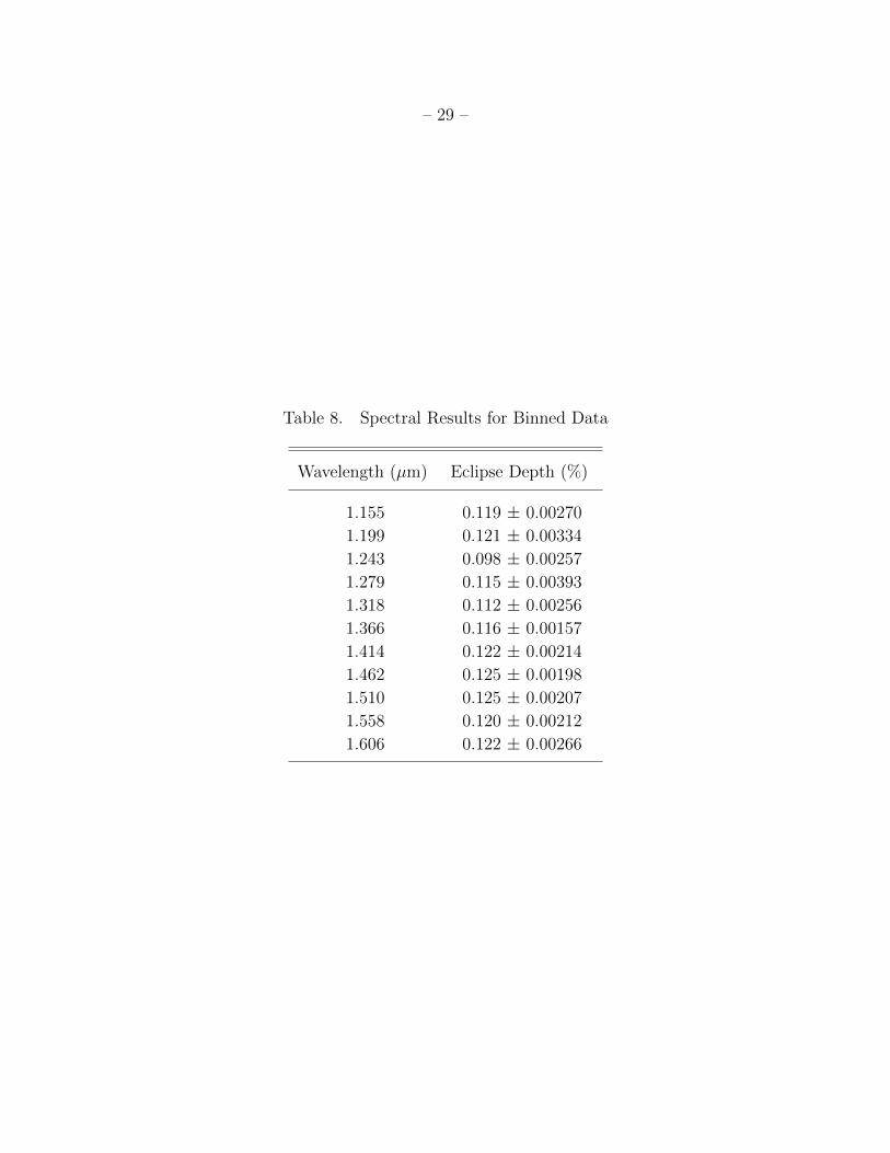
– 29 –

Table 8. Spectral Results for Binned Data

Wavelength (µm) Eclipse Depth (%)

1.155 0.119 ± 0.00270

1.199 0.121 ± 0.00334

1.243 0.098 ± 0.00257

1.279 0.115 ± 0.00393

1.318 0.112 ± 0.00256

1.366 0.116 ± 0.00157

1.414 0.122 ± 0.00214

1.462 0.125 ± 0.00198

1.510 0.125 ± 0.00207

1.558 0.120 ± 0.00212

1.606 0.122 ± 0.00266

– 30 –

Table 9. Error Analysis. We compare photon noise, rms statistics, and both predicted

and measured uncertainties for each source. We show each of these statistics for the

band-integrated time series, binned data, and spectral channels. For the binned data and

spectral channels, the mean uncertainty is shown for each row. The predicted uncertainty

calculation assumes monotonic temporal spacing, which is not the case for WFC3

observations, and is therefore likely to underpredict the true uncertainty. The measured

uncertainty is drawn from the MCMC posterior distributions. The difference between the

predicted uncertainty and the uncertainty from MCMC therefore mostly reflects the

incomplete coverage over the light curve, while the difference between the rms and the

photon noise reflects the impact of additional noise beyond the photon noise.

Parameters Visit 1 Visit 2

Data points during eclipse 38 47

Data points out of eclipse 81 72

Channels

Photon noise (ppm) 419. 420.

RMS of residuals (ppm) 440. 437.

Predicted1 σed (ppm) 79.0 78.0

σed from MCMC+RP Data (ppm) 203. 121.

RMS/photon noise 1.05 1.04

MCMC Data/Pred. 2.57 1.55

0.042-Micron Bins (11 Total)

Photon noise (ppm) 181. 162.

RMS of residuals (ppm) 191. 187.

Predicted1 σed (ppm) 34.0 30.1

σed from MCMC+RP Data (ppm) 76.2 52.6

RMS/photon noise 1.07 1.17

MCMC Data/Pred. 2.33 1.79

Band Integrated Time Series

Photon noise (ppm) 47.3 46.6

RMS of residuals (ppm) 272. 331.

Predicted1 σed (ppm) 9.50 9.58

σed from MCMC+RP Data (ppm) 112. 90.5

RMS/photon noise 5.75 7.10

MCMC Data/Pred. 11.8 9.45

1Calculated from the photon noise and the number of

points during eclipse

– 31 –

REFERENCES

Bean, J. L., Desert, J.-M., Kabath, P., et al. 2011, ApJ, 743, 92

Borysow, A. 2002, A&A, 390

Borysow, A., Jorgensen, U. G., & Zheng, C. 1997, A&A, 324

Cameron, A. C., Guenther, E., Smalley, B., et al. 2010, Monthly Notices of the Royal

Astronomical Society, 407, 507

Castelli, F., & Kurucz, R. L. 2004, arXiv:astro-ph/0

Chen, G., van Boekel, R., Madhusudhan, N., et al. 2014, A&A, 564, A6

Conidis, G. J., Gazeas, K. D., Capobianco, C. C., & Ogloza, W. 2010, Communications in

Asteroseismology, 161, 23

Cowan, N. B., & Agol, E. 2011, The Astrophysical Journal, 726

de Mooij, E. J. W., Brogi, M., de Kok, R. J., et al. 2013, Astronomy & Astrophysics, 550,

A54

Deming, D., Fraine, J. D., Sada, P. V., et al. 2012, The Astrophysical Journal, 754, 106

Deming, D., Wilkins, A., McCullough, P., et al. 2013, The Astrophysical Journal, 774, 95

Desert, J.-M., Vidal-Madjar, A., Lecavelier Des Etangs, A., et al. 2008, A&A, 492, 585

Diamond-Lowe, H., Stevenson, K. B., Bean, J. L., Line, M. R., & Fortney, J. J. 2014, ApJ,

796, 66

Dressel, L. 2012, Wide Field Camera 3, HST Instrument Handbook, Version 5.0

Evans, T. M., Pont, F., Sing, D. K., et al. 2013, ApJ, 772, L16

Fohring, D., Dhillon, V. S., Madhusudhan, N., et al. 2013, MNRAS, 435, 2268

Fortney, J., Lodders, K., Marley, M., & Freedman, R. 2008, The Astrophysical Journal, 678,

1419

Freedman, R. S., Marley, M. S., & Lodders, K. 2008, ApJS, 174, 504

Fressin, F., Knutson, H. a., Charbonneau, D., et al. 2010, The Astrophysical Journal, 711,

374

– 32 –

Gillon, M., Demory, B., Barman, T., et al. 2007, Astronomy and Astrophysics, 471, L51

Guillot, T., Burrows, A., Hubbard, W. B., Lunine, J. I., & Saumon, D. 1996, The Astro-

physical Journal, 459

Hansen, C., Schwartz, J., & Cowan, N. 2014, arXiv preprint arXiv:1402.6699, 1

Herrero, E., Morales, J. C., Ribas, I., & Naves, R. 2011, Astronomy & Astrophysics, 526,

L10

Hoeijmakers, H. J., de Kok, R. J., Snellen, I. A. G., et al. 2014, ArXiv e-prints

Hubeny, I., Burrows, A., & Sudarsky, D. 2003, The Astrophysical Journal, 594, 1011

Huitson, C. M., Sing, D. K., Pont, F., et al. 2013, Monthly Notices of the Royal Astronomical

Society, 434, 3252

Karkoschka, E., & Tomasko, M. 2010, Icarus, 205

Knutson, H. A., Charbonneau, D., Allen, L. E., Burrows, A., & Megeath, S. T. 2008, The

Astrophysical Journal, 673, 526

Knutson, H. a., Howard, A. W., & Isaacson, H. 2010, The Astrophysical Journal, 720, 1569

Kovacs, G., Kovacs, T., Hartman, J. D., et al. 2013, Astronomy & Astrophysics, 553, A44

Kreidberg, L., Bean, J. L., Desert, J.-M., et al. 2014, ApJ, 793, L27

Liddle, A. R. 2004, Monthly Notices of the Royal Astronomical Society, 351, L49

Line, M. R., & Yung, Y. L. 2013, The Astrophysical Journal, 779, 3

Machalek, P., McCullough, P., Burke, C., et al. 2008, The Astrophysical Journal, 684, 1427

Madhusudhan, N. 2012, The Astrophysical Journal, 758, 36

Madhusudhan, N., Mousis, O., Johnson, T. T. V., & Lunine, J. I. J. 2011, The Astrophysical

Journal, 743, 191

Madhusudhan, N., & Seager, S. 2009, The Astrophysical Journal, 707, 24

—. 2010, The Astrophysical Journal, 725, 261

Mandell, A. M., Haynes, K., Sinukoff, E., et al. 2013, The Astrophysical Journal, 779, 128

McCullough, P., & MacKenty, J. 2012, STScI Instrument Science Report WFC3, 1

– 33 –

Moses, J. I., Madhusudhan, N., Visscher, C., & Freedman, R. S. 2013, The Astrophysical

Journal, 763, 25

Parmentier, V., Showman, A. P., & Lian, Y. 2013, Astronomy and Astrophysics, 558, A91

Perez-Becker, D., & Showman, A. P. 2013, ApJ, 776, 134

Rothman, L. S. 2005, Quant Spec. & Rad. Transfer, 96

Sada, P. V., Deming, D., Jennings, D. E., et al. 2012, Publications of the Astronomical

Society of the Pacific, 124, 212

Schwarz, G. 1978, The Annals of Statistics, 6, 461

Schwarz, H., Brogi, M., de Kok, R., Birkby, J., & Snellen, I. 2015, ArXiv e-prints

Showman, A. P., Cooper, C. S., Fortney, J. J., & Marley, M. S. 2008, The Astrophysical

Journal, 685, 1324

Sing, D. K., Lecavelier des Etangs, A., Fortney, J. J., et al. 2013, Monthly Notices of the

Royal Astronomical Society, 436, 2956

Smith, a. M. S., Anderson, D. R., Skillen, I., Cameron, A. C., & Smalley, B. 2011, Monthly

Notices of the Royal Astronomical Society, 416, 2096

Spiegel, D. S., Silverio, K., & Burrows, A. 2009, The Astrophysical Journal, 699, 1487

Stevenson, K. B., Bean, J. L., Fabrycky, D., & Kreidberg, L. 2014, ApJ, 796, 32

Stevenson, K. B., Bean, J. L., Madhusudhan, N., & Harrington, J. 2014, The Astrophysical

Journal, 791, 36

Stevenson, K. B., Harrington, J., Nymeyer, S., et al. 2010, Nature, 464, 1161

von Essen, C., Czesla, S., Wolter, U., et al. 2013, Astronomy & Astrophysics, 561, A48

Wilkins, A. N., Deming, D., Madhusudhan, N., et al. 2014, The Astrophysical Journal, 783,

113

Zahnle, K., Marley, M. S., Freedman, R. S., Lodders, K., & Fortney, J. J. 2009, The Astro-

physical Journal, 701, L20

This preprint was prepared with the AAS LATEX macros v5.2.