speculators, prices and market volatility · daily long and short positions of these traders with...

Bank of Canada staff working papers provide a forum for staff to publish work-in-progress research independently from the Bank’s Governing

Council. This research may support or challenge prevailing policy orthodoxy. Therefore, the views expressed in this paper are solely those of the authors and may differ from official Bank of Canada views. No responsibility for them should be attributed to the U.S. Commodity Futures Trading Commission, the Commissioners or staff at the Commission; the Bank of Canada or other Bank of Canada staff; or the Canadian

government.

www.bank-banque-canada.ca

Staff Working Paper/Document de travail du personnel 2015-42

Speculators, Prices and Market Volatility

by Celso Brunetti, Bahattin Büyükşahin and Jeffrey Harris

2

Bank of Canada Staff Working Paper 2015-42

November 2015

Speculators, Prices and Market Volatility

by

Celso Brunetti,1 Bahattin Büyükşahin2 and Jeffrey Harris3

1Department of Finance Board of Governors of the Federal Reserve System

Washington, DC 20551 Corresponding author: [email protected]

2International Economic Analysis Department

Bank of Canada Ottawa, Ontario, Canada K1A 0G9

Corresponding author: [email protected]

3Department of Finance and Real Estate Kogod School of Business at American University

Washington, DC 20016 [email protected]

ISSN 1701-9397 © 2015 Bank of Canada

ii

Acknowledgements

We would like to thank Kirsten Anderson, Frank Diebold, Michael Haigh, Fabio Moneta,

Jim Moser, James Overdahl, David Reiffen, Michel Robe and Frank Schorfheide. We are

grateful to the seminar participants at the United States Commodity Futures Trading

Commission, the Board of Governors of the Federal Reserve System, Queen’s University

School of Business, the University of Delaware, the University of Mississippi, and

participants at the 16th International Conference of the Society of Computational

Economics for useful discussions and comments. We would also like to thank Kirsten

Soneson for her excellent research assistance. Errors and omissions, if any, are the

authors’ sole responsibility.

iii

Abstract

We analyze data from 2005 through 2009 that uniquely identify categories of traders to

assess how speculators such as hedge funds and swap dealers relate to volatility and price

changes. Examining various subperiods where price trends are strong, we find little

evidence that speculators destabilize financial markets. To the contrary, hedge funds

facilitate price discovery by trading with contemporaneous returns while serving to

reduce volatility. Swap dealer activity, however, is largely unrelated to both

contemporaneous returns and volatility. Our evidence is consistent with the hypothesis

that hedge funds provide valuable liquidity and largely serve to stabilize futures markets.

JEL classification: C3, G1

Bank classification: International topics; Recent economic and financial developments

Résumé

Les auteurs analysent des données de la période 2005-2009, qui distinguent de façon

unique les catégories d’opérateurs, afin d’étudier les relations qui existent entre les

activités des spéculateurs (tels les fonds spéculatifs et les opérateurs sur contrats de swap)

et la volatilité et mouvements des prix. En examinant diverses sous-périodes où les prix

suivaient des tendances marquées, ils constatent qu’à peu près rien n’indique que les

spéculateurs déstabilisent les marchés financiers. Au contraire, les fonds spéculatifs –

dont les opérations reposent sur des rendements contemporains – favoriseraient la

découverte des prix et contribueraient à réduire la volatilité. Les activités des opérateurs

sur contrats de swap, en revanche, ne semblent présenter aucun lien avec les rendements

contemporains et la volatilité. Ces résultats cadrent avec l’hypothèse selon laquelle les

fonds spéculatifs sont d’importants fournisseurs de liquidités et jouent un grand rôle dans

la stabilisation des marchés de contrats à terme.

Classification JEL : C3, G1

Classification de la Banque : Questions internationales; Évolution économique et

financière récente

iv

Non-Technical Summary

As the recent financial crisis demonstrates, failures within the financial system can have devastating effects on the real economy. The crisis has elevated concerns about the trading behavior of financial market participants, particularly those operating outside the public eye. The burgeoning hedge fund industry, for instance, operates largely outside the jurisdiction of the U.S. Securities and Exchange Commission, with few public reporting requirements. Likewise, swap dealers operate in relatively opaque over-the-counter markets, fueling anxiety about their influence as well. In this paper, we analyze the trading of both hedge funds and swap dealers in futures markets from 2005 through 2009 to assess how these traders affect market volatility and prices. We use daily long and short positions of these traders with data from the U.S. Commodity Futures Trading Commission to analyze trading in crude oil, natural gas and corn markets—each of which experienced significant price volatility during the recent crisis. While this volatility was accompanied by increased hedge fund and swap dealer participation, we specifically test for lead-lag and contemporaneous relations between trader positions and both market volatility and prices during various subperiods when prices and volatility were inflated. We find that contemporaneous hedge fund positions were positively correlated with prices but negatively correlated with volatility. These results suggest that hedge funds provide liquidity to the market and facilitate price efficiency. Swap dealer positions, however, are largely unrelated to market returns and volatility. In contrast to the stabilizing influence of hedge funds, merchant positions (in crude oil and natural gas) are significantly positively related to market volatility. These results are consistent with Hirshleifer (1989, 1990), where speculators are drawn to futures markets and the risk premiums are generated by hedging demand from other traders. We also examine whether the “financialization” of futures markets (as represented by the changing mix of participant positions) has affected the functioning of the futures markets. In every instance, we find that speculative position changes do not amplify volatility during the crisis and so do not impede the functioning of futures markets. Conversely, in each market we find that macroeconomic conditions are significantly related to futures market volatility, with the strongest link from 2006 through July 2008. In fact, during the heart of the financial crisis after July 2008, volatility is strongly related to macroeconomic uncertainty (rather than market conditions or financialization). Although our tests do not examine positions, prices or volatility over short intervals (such as a few hours or days), we find no systematic, deleterious link between the trades of hedge funds or swap dealers and either returns or volatility. To the contrary, hedge fund trading, although positively correlated with price changes, is negatively related to volatility both contemporaneously and with a one-day lead. Hedge funds commonly provided liquidity in futures markets and improved price efficiency during the recent financial crisis. We conclude that speculators such as hedge funds and swap dealers should not be viewed as adversarial agents in financial markets, but rather as important liquidity providers to hedgers that enhance the proper functioning of financial markets.

1

1. Introduction

The role of speculators in financial markets has been a source of considerable

interest and controversy in recent years. Concern about speculative trading also finds

support in theory where noise traders, speculative bubbles and herding can drive prices

away from fundamental values and destabilize markets.1 Conversely, traditional

speculative stabilizing theory (Keynes (1923) and Friedman (1953)) suggests that

profitable speculation must involve buying when the price is low and selling when the

price is high so that irrational speculators or noise traders trading on irrelevant

information will not survive in the marketplace. Likewise, Hirshleifer’s (1989, 1990)

speculators are drawn to futures markets by the risk premiums that are generated by

hedging demands.2

The recent financial crisis has elevated concerns about speculators, particularly

those operating outside the public eye, such as hedge funds and swap dealers.

Unregulated hedge funds, for instance, trade a variety of financial products with few

public reporting requirements. Similarly, swap dealers operate in opaque over-the-counter

(OTC) markets but hedge an uncertain fraction of these OTC positions in organized

futures markets. The relative lack of transparency regarding these traders’ activities fuels

anxiety about their influence in regulated financial markets.

Ultimately, the effects of speculative trading in regulated financial markets

become an empirical issue. In this paper, we analyze the trading of both hedge funds and

swap dealers in futures markets from 2005 through 2009 to assess how speculative

trading affects market prices and volatility. The liquid U.S. futures markets offer us a

unique view on this question, having experienced significant price changes with both the

long and short positions of speculative traders easily identified in the data. Indeed, the

U.S. Commodity Futures Trading Commission (CFTC) collects daily position data from

all large market participants, including hedgers (manufacturers, producers and

1 See, for instance, Shleifer and Summers (1990), DeLong et al. (1990), Lux (1995) and Shiller (2003).

Legal efforts to constrain futures speculation focus on traders without direct price risk in the spot asset

(such as hedge funds and swap dealers). The 2010 Dodd-Frank legislation, for example, prescribes specific

oversight for swap dealers and hedge funds. 2 Deuskar and Johnson (2011) demonstrate significant gains to supplying liquidity in the S&P 500 index

futures markets.

2

commercial dealers) and speculators (hedge funds, floor brokers and swap dealers).3 We

analyze three active markets—crude oil, natural gas and corn futures—that have recently

experienced significant volatility and price changes, to assess the impact of speculative

trading.

Both hedge funds and swap dealers have increased exposures to futures markets

during the past decade. Hedge fund market share, for instance, grew more than threefold

in the crude oil markets from 2000 to 2006. Likewise, swap dealers increasingly hedge

their OTC exposure with exchange-traded futures (Büyükşahin et al. (2011)) and also

service most of the burgeoning commodity index fund business. While the market share

of these traders is most important, for illustrative purposes we plot the increase in

speculative open interest (from both swap dealers and hedge funds) in these markets from

2005 through 2009 in Figure 1. Notably, the growth in hedge fund market share from

earlier in the decade levels off during our sample period, but hedge fund and swap dealer

market shares remain high relative to historical levels.

This increased participation has fueled claims that these traders destabilize

markets.4 Indeed, some indirect evidence suggests that trading strategies may have had

some effect on futures prices. For example, Tang and Xiong (2012) show that agricultural

commodities that are part of major commodity indices (the GSCI and DJ-AIG) became

more responsive to macroeconomic shocks post-2004 when index investment rose

dramatically. Commodity index traders (which largely compose our swap dealer

category) announce their trading strategy well in advance and, once they take positions,

these traders typically roll positions forward on pre-announced days. Given this passive

objective, we expect swap dealer position changes to be largely insulated from market

conditions.5

3 We use daily data taken from the CFTC’s Large Trader Reporting System (LTRS), the source of the

CFTC’s weekly Commitment of Traders report (which reports Tuesday closing positions each Friday on

www.cftc.gov). 4 For instance, the Economist (18 June 2008) noted that “The oil market … is behaving like a bucking

bronco again…, politicians are … blaming speculators.” Responding to concerns about speculators, the

CFTC failed to increase position limits for many agricultural futures from 2006 to 2012. 5 Bessembinder, Carrion, Tuttle and Venkataraman (2014), Brunetti and Reiffen (2013) and Mou (2010)

each have evidence related to front-running this roll, with the first paper concluding that other traders

effectively provide liquidity rather than follow predatory strategies, as implied by sunshine trading theories.

3

However, investor flows into commodity index funds may respond to changing

market conditions. Indeed, using extrapolated weekly swap dealer positions from the

CFTC’s Commitments of Traders supplemental reports, Singleton (2014) links investor

flows to futures prices during this time period.6 On the other hand, Irwin and Sanders

(2011) show that Singleton’s inferred data correlate poorly with actual index fund data

reported in the CFTC’s Index Investment Data. Sanders and Irwin (2010, 2011) find little

connection between weekly index investment flows and either prices or volatility.

Likewise, Hamilton and Wu (2014) find no evidence that index trader positions in

agricultural contracts predict returns on nearby futures contracts, and while index trader

positions might help predict changes in oil futures prices from 2007–09, this

predictability appears to be driven by the global financial crisis and breaks down out of

sample.

Capitalizing on the richness of our data, we directly examine daily net swap

dealer and hedge fund positions. We investigate contemporaneous causal links between

trader activity and volatility/returns by adopting an instrumental variable approach. We

find the change in number of accounts reporting to the market to be a valid instrument for

this analysis. To thoroughly empirically assess the effects of speculators and ensure that

our results are robust, we employ several techniques and measures of speculative activity.

Importantly, we isolate three different subperiods for study: the first (covering

2005–07) is characterized by low volatility and stable prices; the second (from 2007

through mid-2008) is characterized by low volatility but rapidly increasing prices; the

third (from mid-2008 through 2009) reflects high volatility with rapidly declining prices.

We examine the run-up and collapse of futures markets to ascertain whether speculative

traders contribute to excessive volatility or to prices overshooting during these periods.

We find that hedge fund position changes are consistently linked to lower

volatility and do not destabilize futures markets. Hedge fund activity is positively related

to contemporaneous returns as well, suggesting that hedge fund participation improves

price discovery.7 Swap dealer position changes, on the other hand, are not consistently

6 Cheng, Kirilenko and Xiong (2014) link macroeconomic risk to futures market investment flows.

7 In the spirit of Hasbrouck (1991), we link concurrent positive return/negative volatility to more efficient

price discovery and surmise (as suggested by an anonymous referee) that if high-speed traders make

markets during the trading day, but avoid overnight positions, hedge funds and other speculators may serve

4

linked contemporaneously to either market volatility or returns.8 Both hedge funds and

swap dealers provide liquidity and enhance price discovery in futures markets during

recent years. These results hold consistently over various subperiods whether prices spike

or bottom out, the very subperiods where excessive volatility and price overshooting have

been alleged.

Importantly, we also find that commercial activity related to the underlying spot

market is strongly connected to volatility and prices. Merchant positions (in crude oil and

natural gas) are significantly positively related to market volatility, a result that stands in

stark contrast to the stabilizing influence of hedge funds.

We also explore whether the “financialization” of futures markets (as represented

by the changing mix of participant positions) has affected the functioning of the futures

markets, as suggested in Singleton (2014) and Cheng, Kirilenko and Xiong (2014).9 In

every instance we find that speculative position changes do not amplify volatility during

the crisis and so do not impede the functioning of futures markets. Conversely, in each

market we find that macroeconomic conditions are significantly related to futures market

volatility, with the strongest link from 2006 through July 2008. In fact, during the depths

of the financial crisis after July 2008, volatility is strongly related to macroeconomic

uncertainty (rather than market conditions or financialization).

Our tests highlight the complexity of trader interactions in futures markets. For

instance, hedge fund, merchant, manufacturer, producer and floor broker positions are all

significantly related to contemporaneous returns. Merchants (in crude oil and natural gas)

bring volatility to these markets, while swap dealers and hedge funds consistently

stabilize these markets, results consistent with Hirshleifer (1989, 1990). Given the fact

that futures contracts exhibit zero sum net positions, these trader interactions are

important. When one group attains a large net position, some other group(s) must take on

as longer-term market makers (see also Brunetti and Reiffen (2013)). Following Lux (1995) and

Lakonishok, Shleifer and Vishny (1992), we find the same results with net speculative position changes and

herding as alternative speculative metrics. 8 Büyükşahin and Harris (2011) find similar lead-lag relations in the crude oil market. Stoll and Whaley

(2010) caution against classifying index investment as speculation and find that index investment has little

price impact on a variety of commodity markets. 9 Barsky and Kilian (2004), Kilian (2007) and Kilian and Vega (2011) examine links between economic

activity, news and shocks, respectively, with commodity prices.

5

the opposite position. It is not evident which trader group drives the overall pattern in any

given market.

Hedge fund trading has been examined during several crisis events, including the

1992 European Exchange Rate Mechanism crisis and the 1994 Mexican peso crisis (Fung

and Hsieh (2000)), the 1997 Asian financial crisis (Brown et al. (2000)), the Long Term

Capital Management financial bailout (Edwards (1999)), and the technology bubble

(Brunnermeier and Nagel (2004) and Griffin et al. (2011)). In some episodes, hedge

funds were deemed to have significant exposures that probably exerted market impact,

while in others they were unlikely to be destabilizing. In contrast, our analysis of detailed

data yields the result that hedge funds consistently stabilize futures markets.10

The remainder of the paper proceeds as follows. In section 2 we describe our data.

In section 3 we analyze the links between trader positions and volatility using an

instrumental variable approach, examine the links between economic activity and

volatility in commodity markets, and concentrate on the links between trader positions

and returns. We conclude in section 4.

2. Data

Our analysis draws upon three different data sets sampled from 3 January 2005

through 19 March 2009: 1) daily futures returns; 2) high-frequency transaction data for

computing realized volatility measures; and 3) daily futures positions of the most

important categories of market participants in these markets.11

The variety across contracts allows us to analyze the role of speculators in

markets that have each experienced dramatic price changes during our sample period. As

Figure 1, Panel A shows, during our sample, crude oil futures rise from about $42 to a

staggering $146 in July 2008 before dropping back to $42 at the end of our sample.

Natural gas futures change dramatically, more than doubling from $6 to $15 at the end of

2005, returning to $6 in 2006, and doubling again to $13 in 2008 before settling below $4

in March 2009. Similarly, corn futures more than double from under $4 to over $8 in

2008 before dropping back near $4 by the end of our sample. For each market, we

10

We provide evidence below in Table II that hedge funds do not simply disappear when volatility

increases, but rather maintain positions on both sides of these markets throughout each subperiod. 11

The New York Mercantile Exchange (NYMEX) crude oil and natural gas contracts represent the largest

energy markets and the Chicago Board of Trade (CBOT) corn futures the largest agriculture market. High-

frequency data for corn begin on 1 August 2006.

6

concentrate on the nearby contract (closest to delivery).12

We present our analysis for

three distinct subperiods, chosen to isolate the effects of trading activity when markets

peak or bottom out. The first subperiod runs from January 2005 (January 2006 for natural

gas and August 2006 for corn) through October 2007 and reflects low volatility with

stable prices. The second subperiod continues through July 2008, a period when

commodity markets experienced moderate volatility with substantial price increases. The

third subperiod continues from July 2008 through 2009, and is characterized by high

volatility with decreasing prices (see Figure 2).

We compute daily returns for each contract using settlement prices set daily by

the exchange at the market close. In particular, we construct daily returns as 𝑟𝑡 = 𝑝(𝑡) −

𝑝(𝑡 − 1), where 𝑝(𝑡) is the natural logarithm of the settlement price on day t. On the

days where we switch contracts from the nearby to the next-to-nearby, both 𝑝(𝑡) and

𝑝(𝑡 − 1) refer to the next-to-nearby contract. In this regard, our smoothed return series

does not include the jumps that commonly occur at contract expiration when contango or

normal backwardation returns can be large (Gorton, Hayashi and Rouwenhorst’s (2014)

“roll yield”). Since the settlement of futures positions is determined by price changes for

individual contracts, and not by differences in prices across contracts, we calculate the

return earned by the long position by omitting contract rollover days. Importantly, the

settlement of futures positions is determined by price changes for individual contracts—

not by differences in prices across contracts. Given the large contango in the energy

markets during our sample period, our average daily returns are smaller than the raw

price series might suggest. For instance, while crude oil prices have risen during our

sample, our mean daily returns are negative, since large “returns” on rollover days are not

included.13

By excluding rollover days, we correctly calculate the return earned by a long

position, and omit “returns” that are not actually earned.

The three markets we examine represent a diverse set of returns over this sample

period. Table I, column 1, reports summary statistics for returns. As noted, mean crude

12

Before expiration, long-term investors roll over positions from the nearby contract to the next-to-nearby

contract, generating seasonality in the data. We consider the nearby contract until its open interest falls

below that of the next-to-nearby contract and explicitly account for seasonality in our tests. Since this

procedure excludes delivery periods, our results are not driven by physical delivery. 13

Bessembinder, Carrion, Tuttle and Venkataraman (2014) discuss various methods for calculating futures

returns with various roll dates, detailing how and why correctly computed futures returns can be negative,

even as spot prices rise, in a contango market.

7

oil returns are negative but have a positive median (the negative mean is due to the sharp

oil price decline in the last subperiod), high standard deviation and mean revert. Natural

gas exhibits significant negative mean daily returns as well, with a very large standard

deviation. Corn displays the highest average daily returns over the sample (6.3 percent

annually).

From intraday CFTC transaction data we construct daily realized volatility

measures. For crude oil and natural gas, we consider transactions from both the electronic

platform and the pit (pit trading declined from 100 to less than 30 percent of volume

during our sample period). In the corn market we utilize only electronic transactions,

since pit trades are commonly reported late, with inaccurate prices, or canceled ex post

throughout our sample period. Each of these futures markets is very liquid—the median

intertrade duration for each is less than one second.

We construct realized volatility measures as follows. Let tp )}({ be the natural

logarithm of the price process over the time interval t, and let tba ],[ be a compact

interval (we use one trading day) partitioned into s subintervals. The ith intraday

subinterval within s is given by 1,[ , ]s s

i i , where 0 1 ...s s s

sa b , and the length of

each intraday interval is given by 1

s s s

i i i . The intraday returns are defined as

1

s s s

i i ir p p where 1,2,..., .i b Realized volatility on day t is the sum of

squared intraday returns sampled at frequency s:

2

1

bs s

t i

i

RV r

. (1)

For each month, we compute s

tRV with s ranging from 1 to 300, in transaction

and calendar time (in seconds). We then examine volatility signature plots each month to

determine optimal sampling frequencies, which range between 30 and 240 trades, in

transaction time, and between 49 and 226 seconds, in calendar time.

Figure 3 reports volatility signature plots in transaction time by averaging the

annualized daily (𝑅𝑉𝑡𝑠)1/2 in each subperiod.

14 Panel A shows that crude oil volatility

14

We compute realized volatility measures only when pit trading is open (9:00 a.m. to 2:30 p.m. EST for

crude oil and natural gas, and 9:30 a.m. to 2:15 p.m. EST for corn). Note that the results in Figure 3 differ

8

stabilizes at 23, 26 and 53 percent in each subperiod, respectively, with the corresponding

sampling frequencies s = 120, 30 and 40 transactions. For natural gas (Panel B), volatility

stabilizes 35, 28 and 45 percent with optimal sampling frequencies s = 120, 30 and 40

transactions during our three subperiods, respectively. While natural gas is more volatile

than crude oil in the first subperiod, crude oil volatility is higher in the third subperiod.

For corn (Panel C), realized volatility stabilizes at 25, 23 and 35 percent with optimal

sampling frequencies of s = 120, 50 and 60 transactions during the three subperiods,

respectively. Overall, we find that these markets are very liquid, with realized volatility

converging to an unbiased level very quickly. We also find that volatility is much higher

for each of these markets during the third subperiod, when commodity prices fell

dramatically.

We adopt four measures of realized volatility: 1) s

tRV with s constant at 120; 2)

s

tRV with s selected optimally each month; 3) the two-scale realized volatility estimator

of Zhang, Mykland, and Aït-Sahalia (2005) with s selected optimally each month; 4) the

kernel estimator of Barndorff-Nielsen, Hansen, Lunde, and Shephard, (2008). The

correlation coefficients between these estimators range from 81% to 95%. We report

results only for s

tRV computed in transaction time with s selected optimally each month

and note that we obtain consistent results using the other realized volatility estimators as

well.

Table I, column 2, provides descriptive statistics for s

tRV . All markets show a

very high average volatility and a high variation in volatility levels. This is perhaps not

surprising, given that our sample is constructed to include markets experiencing dramatic

price changes. Notably, all realized volatility measures are stationary and highly

persistent.

Figure 2 depicts prices and realized volatility for our three markets over time.

Generally speaking, we see marked increases in volatility during periods of market

decline. Our empirical design specifically examines these particular subperiods when the

connection between speculative trading and volatility might be most relevant.

slightly from those reported above because we average realized volatility over each entire subperiod in

Figure 3 but compute optimal sampling frequencies each month in results here.

9

For each market, we obtain individual trader positions from the CFTC’s Large

Trader Reporting System (LTRS), which identifies daily positions of individual traders

classified by line of business.15

LTRS data represent approximately 70 to 90 percent of

total open interest in each market, with the remainder consisting of small traders. The

LTRS data identify growth in speculative positions concurrent with the dramatic swings

in prices for these commodities during our sample period. For example, hedge fund and

swap dealer positions in crude oil markets grew 100 and 50 percent, respectively, during

our sample period.

For each market, we concentrate on the five largest categories of market

participants, with hedge funds and swap dealers common to all three markets. In these

markets we also analyze dealers/merchants (which include wholesalers, exporters-

importers, shippers, etc.) and manufacturers (for crude oil and corn, including fabricators,

refiners, etc.) or producers (for natural gas).

Given our focus on the effects of speculation, we specifically analyze the

positions of commodity swap dealers and hedge funds. Hedge fund complexes are

registered with the CFTC as Commodity Pool Operators, Commodity Trading Advisors,

and/or Associated Persons who may control customer accounts. CFTC market

surveillance staff also identify other hedge funds that are known to be managing money

for customers.16

Swap dealers use derivative markets to manage price exposure from

OTC swaps and transactions with commodity index funds.17

Table II shows that our five trader categories comprise between 52 and 100

percent of the total open interest in each market, on the average trading day. Merchants,

producers and manufacturers are primarily short, consistent with the hedging objectives

of these participants in futures markets. Swap dealers hold an average of approximately

40 percent of long positions, consistent with large long positions taken on behalf of

commodity index funds. Interestingly, hedge fund positions are more heterogeneous than

other traders, holding large positions on both the long and short sides of all three markets.

15

CFTC reporting thresholds (350 contracts for crude oil, 200 contracts for natural gas and 250 contracts

for corn) balance between effective surveillance and reporting costs. 16

For completeness, we corroborate our hedge fund sample with fund characterizations in the press. 17

Index funds are increasingly used by large institutions to diversify portfolios with commodities—in June

2008, the notional value of commodity index investments tied to U.S. futures exchanges exceeded

$160 billion.

10

In Panel A of Table II, comparing the first subperiod (stable prices and low

volatility) to the second subperiod (rising prices and low volatility), hedge funds move to

sell more than they buy (short positions increase from 21% to 25%, while long positions

move from 23% to 24%). In other words, while prices are increasing, hedge funds sell

more and stabilize prices. Hedge funds maintain a significant presence in the crude oil

market, and swap dealer positions remain stable at 42% of long open interest throughout

these periods.

In Panel B for natural gas, hedge funds increase their short positions from

subperiod 1 (57%) to subperiod 2 (64%) when prices are rising, again stabilizing market

prices. While hedge fund short positions increase from 64% to 68% from subperiod 2 to 3

(when prices are falling), the concurrent increase in long hedge fund positions is larger

(increasing from 28% to 37%), again stabilizing market prices. Interestingly, swap

dealers decreased their long position from 45% to 34% of long open interest from

subperiod 1 to subperiod 2, precisely when swap dealers were blamed for driving up the

prices.

Figure 1 displays the time-series plot of the 44-day moving average of total open

interest (long plus short positions) held by each of our trader categories, along with

market prices, noting that this metric captures increased participation, but not necessarily

larger net positions. Both swap dealers and hedge funds increase positions over our

sample period (although not monotonically through time) in the crude oil and natural gas

markets. In the corn market, however, both swap dealers and hedge funds reduce

aggregate positions during our sample period.

For our empirical tests, we consider the daily change in the number of contracts

held in long (or short) positions, the change in net futures positions (futures long minus

futures short), and the change in net total positions (the sum of net futures positions and

the net delta-adjusted option positions) of each trader category in each market. Since

results based on these three variables are similar, we present results for the daily change

in net futures positions.

Columns 3 through 7 in Table I show descriptive statistics for daily changes in the

net futures positions by market participant and market. In crude oil and natural gas

markets, both mean and median swap dealer position changes are positive, indicating an

11

overall increase in their net long positions. Hedge fund net position changes in crude oil

and natural gas are negative. For corn, the net positions of both swap dealers and hedge

fund positions decrease over time. All position changes are stationary.

Table III reports correlation coefficients among trader positions. Note that both

the sign and significance of these correlations are similar during each subperiod,

reflecting the stable role these participants play in futures markets. Merchant positions are

positively correlated to manufacturer (producer for natural gas) positions, consistent with

these commercial traders having common trading interests. Conversely, hedge fund and

swap dealer positions are negatively correlated to merchant and manufacturer positions,

consistent with risk transfer among these participants.

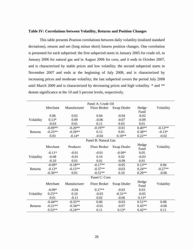
Table IV reports the correlations between position changes and both volatility and

returns, by subperiod. Very few subperiods display any significant correlations between

trader positions and volatility (except that merchant position changes are significantly

positively correlated with volatility in four of nine subperiods). Importantly, speculative

position changes are rarely correlated with volatility, and when significant, this

correlation is negative.

Hedger position changes (merchants, producers and manufacturers) are negatively

correlated with market returns. Similarly, floor broker position changes, when significant,

are negatively correlated with natural gas and crude oil returns, indicating that floor

brokers provide liquidity and trade against price trends. The correlations between

speculative trader positions and returns are distinctly different. Consistent with the

passive nature of commodity index investing, swap dealer positions are largely

uncorrelated with returns. Hedge fund position changes, however, are significantly

positively correlated with market returns, suggesting that hedge funds, in the aggregate,

are momentum traders.

The last column of Table IV reports the correlation coefficient between returns

and volatility in each subperiod. When significant, this correlation is always negative,

consistent with documented evidence from other markets.18

Interestingly, in the last

subperiod, when volatility is high as prices are dropping, the correlation between

volatility and returns is not statistically significant.

18

Andersen, Bollerslev, Diebold, and Ebens (2001) review the literature on this negative relation.

12

3. Trader Position Changes and Volatility

We first explore whether various traders are related to contemporaneous volatility

with an instrumental variable approach.

3.1 The Instrument: The Change in the Number of Reporting Accounts

While the contemporaneous correlations between position changes and both

returns and volatility are suggestive, these relations may not be causal. To explore

causality we adopt an instrumental variable approach. The choice of the instrument is

obviously important—a valid instrument must be correlated to trader positions, but not

correlated to volatility (or returns). We examine a number of potential instruments,

ultimately using the change in the total number of accounts reporting positions in each

market each day.

The change in the total number of accounts reporting to the market each day has

the desired correlation with trader positions (supported by tests reported in Table V

below). Traders with large positions, denominated by the number of long or short

contracts held, are required to report to the CFTC each day. The cost of reporting

positions to the CFTC is not trivial and requires registration, compliance systems and

staff, etc. Importantly, traders near the reporting threshold almost always report daily

positions on a routine basis, rather than starting and stopping the reporting process when

they cross the reporting thresholds at the margin. Over longer horizons, however, traders

falling below reporting thresholds more often stop reporting. This dynamic keeps the

number of reporting accounts correlated with trader positions, but keeps the number of

reporting accounts largely exogenous with respect to market volatility (and returns).

We find consistent evidence that large traders routinely report positions to the

CFTC even during the most volatile market conditions, and therefore sporadic position

reporting based on market volatility does not influence our instrument. We argue that the

daily change in the number of reporting accounts is thus largely predetermined and

unrelated to daily volatility, making it a valid instrument.

Importantly, position reporting thresholds are set as a number of contracts, so that

market prices do not play a direct role in whether an account is required to report, and

thus prices are unrelated to our instrument as well. In this regard, there is no systematic

13

link between the number of reporting accounts and returns. We provide formal tests of

the instrument’s validity for each market and subperiod.

The last column of Table I displays descriptive statistics of our instrument. As

noted above, despite the considerable changes in these markets over our sample period,

the average number of reporting accounts is stable over time—the time series of the

instrument is stationary. In fact, the mean daily change in reporting accounts is zero, with

median changes of -1 for crude oil and natural gas, and zero for corn.

Figure 4 presents time-series plots of the instrument for each market over the full

sample period. Note that while the three subperiods are chosen to represent significant

differences in the levels and volatility of prices, our instrument remains relatively stable

across the full sample period. The change in the number of reporting accounts is not

significantly linked with either volatility or returns.

The correlation between our instrument and trader positions is not very high. The

first-stage regressions of the instrument on trader positions yield an average R2 around

2%. Hence, the change in trader positions is a weak instrument, which may bias our

estimated parameters and produce unreliable standard errors. To overcome this potential

problem, we adopt the Stock and Yogo (2005) procedure (described in detail in Appendix

B) to test the validity of the instrument.

Note that Figure 4 reveals some large daily movements in the instrument that may

affect the correlation between the instrument and trader positions.19

To check for this

possibility, we examine whether these large movements affect these correlations. In fact,

the correlation between the instrument and the endogenous variables increases if we trim

the large values of the instrument and our results are robust to those large movements.

3.2 Volatility – Trading Activity Causality

We test for a contemporaneous causal relation between realized volatility and

trader positions using the heterogeneous autoregressive model of realized volatility

(HAR-RV) developed by Corsi (2009). The model captures both short-term and long-

term dynamics of the volatility process by accounting for realized volatility at different

19

We thank an anonymous referee for pointing this out.

14

frequencies.20

This feature is very important, since the volatility process exhibits both

clustering (i.e., short-term dependence) and long memory (long-term dependence). The

HAR-RV model can be written as

(𝑅𝑉𝑖,𝑡𝑑 )

1

2 = 𝛼𝑖 + 𝛾𝑑(𝑅𝑉𝑖,𝑡−1𝑑 )

1

2 + 𝛾𝑤(𝑅𝑉𝑖,𝑡−1𝑤 )

1

2 + 𝛾𝑚(𝑅𝑉𝑖,𝑡𝑚)

1

2 + 𝛽𝑖𝑗|∆𝑇𝑃𝑖,𝑡

𝑗| + 휀𝑖,𝑡 , (2)

where 𝑅𝑉𝑖,𝑡𝑑 is the daily realized volatility in market i on day t computed by optimally

sampling over s observations; 𝑅𝑉𝑖,𝑡−1𝑤 is the weekly realized volatility computed as the

simple arithmetic average of the daily 𝑅𝑉𝑖,𝑡𝑑 over the past five days; similarly, 𝑅𝑉𝑖,𝑡

𝑚 is the

monthly realized volatility computed as the average daily realized volatility in the past

month (22 days); |∆𝑇𝑃𝑖,𝑡𝑗

| is the absolute value of position changes of trader group j in

market i on day t; 휀𝑖,𝑡 is an error term assumed to be uncorrelated with realized volatility

but not necessarily with |∆𝑇𝑃𝑖,𝑡𝑗

|. We are particularly interested in 𝛽𝑖𝑗, which measures the

contemporaneous impact of the trading activity of trader group j on volatility in market i.

We estimate equation (2) with the two-stage weak instrumental variable approach

of Stock and Yogo (2005). The first stage consists in testing the validity of the

instrument. In the case of a single instrument, Stock and Yogo (2005) (following Staiger

and Stock (1997)) show that this test is simply the F-test of the regression of the variable

of interest (absolute value of position changes) on the instrument (the change in the

number of reporting accounts).21

The second stage consists in estimating equation (2)

using limited information maximum likelihood (LIML).

Table V displays the results of the LIML instrumental variable along with the F-

test of the first-stage regression.22

The first-stage results support our contention that the

change in the number of reporting accounts is a valid instrument, with 50 of the 60

regressions resulting in an F-test exceeding the critical value of 8.96. The change in the

number of reporting accounts is a valid instrument in 19 crude oil regressions, 18 natural

gas regressions and 13 corn regressions.

20

For further details about the HAR-RV model, see Appendix A. 21

Stock and Yogo (2005) derive more accurate critical values for the F-test under weak instruments, which

differ from the standard F-test critical values. 22

LIML is less sensitive to weak instruments than two-stage least squares estimation. In order for the actual

size of the F-test to be no greater than 10% (15%), the F-statistics should exceed 16.38 (8.96).

15

Table V also shows the relation between various position changes and volatility.

Merchant position changes are always significantly related to volatility in both the crude

oil and natural gas markets across the full sample and in all subperiods. In these energy

markets the largest coefficient on merchant position changes occurs during the last

subperiod when volatility was very high. To put our estimates in perspective, in the last

subperiod, for every 1,000 contracts traded by merchants, volatility increased by 0.11%

and 1.1% in crude oil and natural gas, respectively. Merchants are not as important to

corn volatility, with merchants significant only in the first and second subperiods with

relatively small coefficients.

Manufacturers and producers are never important to volatility in the crude oil and

natural gas markets. In corn, manufacturer position changes are significant only during

the last subperiod when volatility is high, increasing volatility by 0.3% for every 1,000

contracts traded.

Floor brokers are significantly related to volatility in both crude oil and natural

gas, but have little impact on corn volatility (except during the first subperiod). Similar to

the effects of commercial traders described above, the trading activity of floor brokers,

when significant, always increases contemporaneous volatility.

Conversely, we find that the effects of speculator activities are distinctly

different––hedge fund position changes significantly reduce contemporaneous volatility

in crude oil and natural gas markets and in corn during the last, high-volatility subperiod.

Over the full sample, hedge funds reduce volatility by 0.06% and 0.04% for every 1,000

contracts traded in crude oil and natural gas, respectively. Hedge funds are important

liquidity providers in these markets, taking positions that mitigate contemporaneous

market volatility.

Consistent with the fact that swap dealer positions proxy for relatively passive

index fund traders, swap dealer position changes are generally unrelated to

contemporaneous volatility. Interestingly, swap dealer trading significantly reduces

volatility in the natural gas market during the third, high-volatility subperiod. In general,

hedgers, and not speculators, are more consistently linked to futures market volatility.

These tests highlight the distinct lack of connection between speculative positions

and inflated market volatility––no specification links speculative trader activity to higher

16

volatility in any subperiod. To the contrary, hedge fund activity significantly reduces

volatility in all subperiods for crude oil and during the 2008 run-up in natural gas prices.

Notably, swap dealer activity is unrelated to volatility, consistent with the passive nature

of commodity index fund investment. When significant during the 2008 corn market run-

up, swap dealer activity also reduced volatility levels.

3.3 Volatility and Economic Activity

Historically, commodity futures markets allow buyers (i.e., manufacturers) and

sellers (i.e., producers of the commodity) to hedge their natural spot exposures, linking

real economic activity with financial markets. Recent work, however, posits that the post-

2006 “financialization” of commodity markets helps explain increases in commodity

price volatility (Tang and Xiong (2012)) and price changes (Henderson, Pearson and

Wang (2012)). Cheng, Kirilenko and Xiong (2014), Singleton (2014), and Tang and

Xiong (2012) suggest that the link between economic activity and financial markets has

evolved over time, so we examine this link over each of our subperiods.

To account for the current state of the economy, we use the Arouba, Diebold and

Scotti (2009) (ADS) index, which tracks real business conditions. Updated weekly by the

Federal Reserve Bank of Philadelphia, the ADS index is based on six macroeconomic

indicators including weekly initial jobless claims, monthly payroll employment, industrial

production, personal income less transfer payments, manufacturing and trade sales, and

quarterly real GDP. The index accounts for high- and low-frequency information with

both stock and flow data. By construction, the average ADS index is zero, with

progressively larger values indicating better-than-average economic conditions, and

greater negative values indicating progressively worse-than-average conditions.

Of course, the recent financial crisis has had demonstrable impact on financial

markets worldwide. Indeed, the economic uncertainty that characterized financial markets

during the crisis is likely to feed directly into the commodity markets we study. Bloom

(2009), for instance, shows that higher uncertainty causes firms to reduce investment and

hire fewer workers. Leduc and Liu (2012) show that uncertainty in the recent crisis has

reduced economic activity more than in previous recessions. Therefore, we also consider

the Scotti (2013) uncertainty index as a straightforward and intuitive measure of

17

uncertainty in the economy. Higher (lower) index levels indicate that agents are more

(less) uncertain about the state of the economy.

Figure 5 depicts the ADS business conditions index along with the Scotti

uncertainty index. As shown, the ADS index fluctuates around zero in the first subperiod,

becomes negative in the second subperiod at the onset of the recession and drops further

in the last subperiod during the financial crisis. The uncertainty index, on the other hand,

remains stable through the first two subperiods, but spikes at the onset of the last

subperiod and remains high, reflecting the extreme uncertainty during the recent

recession.

We estimate the effect of economic activity and uncertainty on commodity market

volatility using the same approach as in equation (2):

𝑙𝑛 [(𝑅𝑉𝑖,𝑡𝑑 )

1

2] = 𝑎𝑖 + 𝑔𝑑𝑙𝑛 [(𝑅𝑉𝑖,𝑡−1𝑑 )

1

2] + 𝑔𝑤𝑙𝑛 [(𝑅𝑉𝑖,𝑡−1𝑤 )

1

2] + 𝑔𝑚𝑙𝑛 [(𝑅𝑉𝑖,𝑡𝑚)

1

2] + 𝑏𝑖𝐸𝐴𝑡 + 𝑒𝑖,𝑡 ,(3)

where 𝐸𝐴𝑡 refers to the ADS and uncertainty indices, respectively. We use the log-

realized standard deviation, since the ADS index takes positive and negative values.

We estimate equation (3) during each subperiod, exploring the link between

economic activity and the volatility of major commodity markets, and whether this link

has changed over time. We report the results for each market in Table VI. For the full

sample, commodity market volatility is significant and negatively linked to the ADS

index, indicating that worsening U.S. business conditions increase volatility in

commodity markets. Notably, the parameter estimates are similar across the crude oil,

natural gas and corn markets. As expected, this result reinforces the strong link between

economic activity and commodity markets.

In the first subperiod (with low volatility and stable economic conditions), the link

between business conditions and volatility is negative, but significant only for crude oil

and natural gas. During the second subperiod, when commodity prices are rising but

volatility is stable, the link is negative and highly significant. Note that during this second

subperiod, U.S. business conditions deteriorate but commodity prices rise, reflecting

world demand (Bodenstein and Guerrieri (2011)).

During our third subperiod, when the economic crisis becomes very severe,

commodity prices fall dramatically and volatility is very high. Perhaps surprisingly,

18

during this subperiod, the ADS index becomes statistically unimportant. However, the

reduced real economic activity associated with higher uncertainty translates into higher

futures market volatility during the crisis. Overall, we find a strong link between

economic activity and commodity price volatility. While during the recent crisis the link

shifts from business conditions (measured by the ADS index) to economic uncertainty,

we find no evidence that the “financialization” of commodity markets breaks the link

between the real economy and these markets.

3.4 Trader Position Changes and Returns

The correlations in Table VII suggest a link between market prices and

speculative activity (noted also in popular press articles). We explore the possible link

between trader position changes and returns with tests for a contemporaneous causal

relation with the following equation:

𝑅𝑖,𝑡 = 𝜗𝑖 + ∑ 휁𝑖,𝑘𝑅𝑖,𝑡−𝑘 + 𝜅𝑖𝑗∆𝑇𝑃𝑖,𝑡

𝑗+ 𝜈𝑖,𝑡

5𝑘=1 , (4)

where Ri,t is the daily futures return in market i on day t, ∆𝑇𝑃𝑖,𝑡𝑗

is the position changes of

trader group j in market i on day t, and 𝜈𝑖,𝑡 is an error term assumed to be uncorrelated

with the return process but not necessarily with ∆𝑇𝑃𝑖,𝑡𝑗

. The five lagged returns (Ri,t) cover

the trading days of the past week. As above, we estimate equation (4) using LIML.23

As Table VII shows, merchant and manufacturer position changes, when

significant, are negatively related to contemporaneous returns in the crude oil and corn

markets. These trading patterns suggest that merchants and manufacturers are contrarian

traders. Recall from Table V, however, that these traders are also linked to higher

contemporaneous volatility, so they do not act as effective liquidity providers in their

contrarian role.

The relation between prices, volatility and merchant/manufacturer position

changes merits further discussion. Recall from Table II that merchants and manufacturers

are primarily short (particularly in crude oil). One possibility is that these commercial

traders act as price takers, actively adjusting hedged positions based on contemporaneous

returns by increasing short positions to lock in future prices when prices rise and

23

Note that in equation (2) we consider the absolute value of position changes, while in equation (4) we use

position changes. Hence, we repeat the Stock and Yogo test for the validity of the instrument.

19

liquidating short positions when prices fall. A second possibility is that hedge funds and

swap dealers abandon the market when volatility increases. However, we find relatively

little change in the positions held by hedge funds and swap dealers from subperiod to

subperiod, suggesting that the dynamic is driven more by commercial traders reacting to

price changes.

In natural gas, the relation between merchant position changes and

contemporaneous returns is not as stable, with both significantly positive and negative

relations across our various subperiods. Merchant position changes are positively related

to price changes during the run-up of natural gas prices, but negatively related to price

changes when natural gas prices fall during 2008–09. Producer position changes are less

significantly related to contemporaneous returns, and significantly negative only in our

first subsample, when prices are relatively stable.

Notably, swap dealers are rarely significantly related to contemporaneous returns,

except during our third subperiod, when prices for all three commodities are falling.

During this subperiod, swap dealer position changes are positively related to

contemporaneous returns, albeit with marginal significance. This is in line with a

reduction in swap dealer positions in the last subperiod, documented in Figure 1. The lack

of connection between swap dealer positions and contemporaneous price changes,

especially during the run-up of commodity prices, is consistent with the relatively passive

role that swap dealers play in these markets—they bring long-only index fund money to

these markets, flows that do not appear to be sensitive to daily price changes.

Hedge fund position changes, however, are significantly related to returns in all

markets. In both crude oil and corn markets, hedge funds appear to consistently move in

the same direction as prices, but do so in a manner that reduces volatility (as shown

above), suggesting that hedge fund participation improves price discovery. In the natural

gas market, the relation (again) is more complex—hedge funds trade with the trend

during the first and third subperiods, but against the trend when natural gas prices are

rising during the second subperiod. Over the full sample, hedge funds trade against

contemporaneous natural gas returns. These results highlight the diversity of hedge fund

trading strategies across these different futures markets, so that conclusions drawn about

20

hedge funds from one commodity market should not be considered robust to all other

markets.

4. Conclusion

We first explore whether various traders are related to contemporaneous volatility

with an instrumental variable approach.

We employ a unique data set that allows us to precisely identify positions of

market participants in three actively traded and recently volatile futures markets to

investigate whether speculation increases market volatility or moves prices. Examining

correlations and contemporaneous effects with instrumental variables, we find that hedge

fund position changes are consistently linked to reduced volatility and do not destabilize

futures markets. Hedge fund activity is positively related to contemporaneous returns as

well, suggesting that hedge fund participation improves price discovery in these markets.

Swap dealer position changes, on the other hand, are not consistently linked

contemporaneously to either market volatility or returns.

We also provide evidence that the links between real economic activity and

commodity prices remain intact during the recent financial crisis. While economic

conditions are significantly linked to commodity price volatility prior to the financial

crisis, economic uncertainty drives commodity price volatility after July 2008. These

robust connections cast doubt on conjectures that increased “financialization” of

commodity markets has altered the dynamics of commodity markets during the recent

financial crisis. Rather, during the crisis, position changes and volatility are both driven

by macroeconomic uncertainty, and position changes per se do not cause volatility.

Consistent with hedging pressure theories, we find that commercial activity

related to the underlying futures market is commonly connected to volatility and prices.

Merchant positions are significantly positively related to market volatility, a result that

stands in stark contrast to the stabilizing influence of hedge funds and swap dealers.

Importantly, these results hold consistently across various commodity futures

products during the recent financial crisis that generated historically high volatility levels.

Indeed, our results hold for various subperiods when prices trend upward, downward or

reverse sharply. While we present results for net position changes for various trader

groups, our results are also robust to alternative volatility metrics and speculative

21

measures, such as the daily change in the number of contracts held in long (or short)

positions and the change in net total positions (the sum of net futures positions and the

net delta-adjusted option positions).

Our results are consistent with Deuskar and Johnson’s (2011) conjecture that

investors with constant risk tolerance (hedge funds, perhaps) can trade profitably against

flow-driven shocks. In this light, the increasing positions taken by hedge funds and swap

dealers in futures markets during recent years may simply reflect a rational profit motive,

with their positions enhancing price discovery during the recent financial crisis.

These results are important for both researchers and policy-makers alike. For

researchers, we demonstrate that the trades of relatively unconstrained traders who

primarily process fundamental information can reduce market volatility by taking

positions opposite to commercial entities with hedging needs. For policy-makers, these

results show that hedge fund participation can benefit financial markets, and they

highlight the benign influence of the growing commodity index positions in futures

markets. Our results should give pause to those who seek to limit speculative trading

based on the observation that positions have been growing.

Of course, the prospect that speculators destabilize markets is real (see models by

Shleifer and Summers (1990), DeLong et al. (1990), Lux (1995) and Shiller (2003),

among others), and effective regulation of these entities is certainly merited. Although we

do not rule out the possibility that traders might attempt (or actually succeed) to move

prices and magnify volatility over short time intervals (such as minutes or hours), we find

no evidence of this phenomenon during various months-long run-ups or declines that

characterize recent commodity prices. Our tests show that there has been no systematic,

deleterious link between the trades of hedge funds or swap dealers and either returns or

volatility during recent years. Hedge fund trading, in fact, can be linked to returns, but in

a beneficial sense—hedge funds trade in the same direction as price changes, but reduce

volatility, a pattern consistent with improving price discovery in financial markets.

22

Table I: Descriptive Statistics

This table presents mean, median, standard deviations and the DF-GLS stationary test of Elliott, Rothenberg, and Stock (1996) for

daily returns, volatility (realized standard deviation), and daily net (long minus short futures) trader position changes for the full sample. For

the crude oil and natural gas markets, the sample extends from January 2005 through March 2009. For the corn market, the sample extends

from August 2006 through March 2009. ΔNRA refers to the change in the number of reporting accounts, our instrument applied in equations

(2) and (4). AC(1) refers to the autocorrelation coefficient of order 1. The DF-GLS tests the null of non-stationarity with critical values

-1.941 and -1.616 at the 5% and 10% levels, respectively (see MacKinnon, 1996).

Panel A: Crude Oil – Full Sample – 1047 obs.

Returns (%) Volatility (%) Merchant Manufacturer Floor Broker Swap Dealer Hedge Fund ΔNRA

Mean -0.046 28.76 -64.21 512.7 146.6 159.7 -1,285 0.000

Median 0.059 24.71 306.0 272.0 18.00 492.0 -1,295 -1.000

Std. Dev. 2.514 13.84 6,783 3,162 2,229 8,208 6,644 7.794

AC(1) -0.088 0.840 0.344 0.285 -0.050 0.470 0.006 0.014

DF-GLS -2.410 -1.543 -21.32 -2.748 -33.11 -19.37 -2.572 -2.089

Panel B: Natural Gas – Full Sample – 1053 obs.

Returns (%) Volatility (%) Merchant Producer Floor Broker Swap Dealer Hedge Fund ΔNRA

Mean -0.188 35.58 89.89 6.549 64.73 381.8 -70.39 0.000

Median -0.157 33.28 26.00 0.000 39.00 51.00 -246.0 -1.000

Std. Dev. 3.056 14.94 1,429 428.4 1,442 2,867 3,423 7.100

AC(1) 0.024 0.386 0.250 0.263 -0.129 0.531 0.156 -0.004

DF-GLS -2.433 -6.350 -3.299 -12.95 -5.863 -17.07 -27.48 31.90

Panel C: Corn – Full Sample – 646 obs.

Returns (%) Volatility (%) Merchant Manufacturer Floor Broker Swap Dealer Hedge Fund ΔNRA

Mean 0.025 27.24 868.2 -116.6 -208.0 -328.7 -362.8 0.000

Median 0.000 25.80 830.5 -152.5 -151.5 -620.0 -423.3 0.000

Std. Dev. 2.303 9.236 6,669 1,400 4,191 7,937 6,918 12.09

AC(1) 0.015 0.595 0.385 0.097 0.237 0.623 0.183 0.089

DF-GLS -24.51 -1.978 -5.213 -6.282 -4.476 -7.202 -21.05 -22.99

23

Table II: Long and Short Positions as Fraction of Total Open Interest

This table presents daily average long and short positions expressed as a fraction

of total open interest, by trader, with the daily Total Mean, Maximum, and Minimum

referring to the sum of daily fractions across the five trader categories in each market. For

the crude oil and natural gas markets, the sample extends from January 2005 through

March 2009. For the corn market, the sample extends from August 2006 through March

2009.

Panel A: Crude Oil

Full sample

Total

Merchant Manufacturer Floor

Broker

Swap

Dealer

Hedge

Funds

Mean Max Min

Long 0.07 0.01 0.02 0.42 0.23 0.75 0.88 0.52

Short 0.30 0.10 0.05 0.06 0.22 0.73 0.85 0.58

Subperiod 1: Stable prices, low volatility 01/03/2005 – 10/31/2007

Long 0.09 0.01 0.02 0.42 0.23 0.77 0.88 0.61

Short 0.31 0.12 0.05 0.05 0.21 0.74 0.85 0.58

Subperiod 2: Rising prices, low volatility 11/01/2007 – 07/03/2008

Long 0.05 0.01 0.02 0.42 0.24 0.74 0.81 0.78

Short 0.26 0.07 0.04 0.08 0.25 0.70 0.75 0.67

Subperiod 3: Falling prices, high volatility 07/08/2008 – 03/19/2009

Long 0.05 0.01 0.02 0.42 0.22 0.71 0.76 0.74

Short 0.26 0.06 0.05 0.10 0.25 0.73 0.68 0.65

Panel B: Natural Gas

Full sample

Total

Merchant Producer Floor

Broker

Swap

Dealer

Hedge

Funds

Mean Max Min

Long 0.07 0.01 0.02 0.39 0.29 0.78 0.91 0.62

Short 0.16 0.03 0.05 0.07 0.57 0.87 1.00 0.69


Long 0.07 0.01 0.01 0.45 0.24 0.78 0.70 0.65

Short 0.13 0.02 0.05 0.09 0.57 0.86 0.88 0.83


Long 0.05 0.00 0.02 0.34 0.28 0.81 0.80 0.68

Short 0.11 0.03 0.05 0.04 0.64 0.87 0.86 0.77


Long 0.06 0.01 0.04 0.30 0.37 0.79 0.71 0.69

Short 0.09 0.01 0.05 0.04 0.68 0.87 0.88 0.85

24

Panel C: Corn

Full sample

Total

Merchant Manufacturer Floor

Broker

Swap

Dealer

Hedge

Funds

Mean Max Min

Long 0.05 0.03 0.06 0.41 0.20 0.76 0.85 0.61

Short 0.44 0.05 0.09 0.02 0.16 0.75 0.85 0.63


Long 0.05 0.03 0.05 0.45 0.19 0.77 0.85 0.71

Short 0.44 0.05 0.09 0.01 0.17 0.76 0.84 0.69


Long 0.05 0.04 0.06 0.43 0.22 0.80 0.84 0.71

Short 0.51 0.04 0.07 0.01 0.13 0.77 0.81 0.72


Long 0.07 0.03 0.07 0.32 0.19 0.69 0.79 0.61

Short 0.36 0.04 0.09 0.03 0.18 0.71 0.77 0.63

25

Table III: Correlations between Trader Position Changes

This table presents Pearson correlations between net (long minus short) futures

position changes across traders. One correlation is presented for each subperiod: the first

subperiod starts in January 2005 for crude oil, in January 2006 for natural gas and in

August 2006 for corn, and it ends in October 2007, and is characterized by stable prices

and low volatility; the second subperiod starts in November 2007 and ends at the

beginning of July 2008, and is characterized by increasing prices and moderate volatility;

the last subperiod covers the period July 2008 until March 2009 and is characterized by

decreasing prices and high volatility. * and ** denote significance at the 10 and 5 percent

levels, respectively.

Panel A: Crude Oil

Merchant Manufacturer Floor Broker Swap Dealer

Manufacturer 0.27** 0.18**

0.30**

Floor Broker

0.05

-0.05 -0.01

0.04

-0.04 0.11

Swap Dealer

-0.66**

-0.62** -0.62**

-0.42**

-0.44** -0.31**

-0.22**

-0.00 -0.13*

Hedge Fund

-0.25**

-0.13*

-0.27**

-0.25**

-0.11

-0.32**

-0.15**

-0.11

-0.08

-0.20**

-0.38**

-0.27**


Merchant Producer Floor Broker Swap Dealer

Producer 0.12** 0.15*

-0.37**

Floor Broker

0.12**

0.19** 0.23**

0.08

0.16** 0.02

Swap Dealer

-0.42**

-0.33** -0.13*

-0.16**

-0.46** 0.06

-0.23**

-0.19** -0.20**

Hedge Fund

0.09*

-0.14* -0.17**

-0.07

0.12 -0.19**

-0.18**

-0.31** -0.53**

-0.71**

-0.61** -0.44**

Panel C: Corn

Merchant Manufacturer Floor Broker Swap Dealer

Manufacturer 0.44** 0.30**

0.22**

Floor Broker 0.07 0.07

-0.12

0.05 0.00

-0.02

Swap Dealer

-0.53**

-0.64** -0.33**

-0.27**

-0.15** -0.31**

-0.52**

-0.38** -0.38**

Hedge Fund

-0.51**

-0.53** -0.47**

-0.33**

-0.36** -0.24**

-0.07

-0.18** -0.04

-0.18**

-0.03 -0.14*

26

Table IV: Correlations between Volatility, Returns and Position Changes

This table presents Pearson correlations between daily volatility (realized standard

deviations), returns and net (long minus short) futures position changes. One correlation

is presented for each subperiod: the first subperiod starts in January 2005 for crude oil, in

January 2006 for natural gas and in August 2006 for corn, and it ends in October 2007,

and is characterized by stable prices and low volatility; the second subperiod starts in

November 2007 and ends at the beginning of July 2008, and is characterized by

increasing prices and moderate volatility; the last subperiod covers the period July 2008

until March 2009 and is characterized by decreasing prices and high volatility. * and **

denote significance at the 10 and 5 percent levels, respectively.

Panel A: Crude Oil

Merchant Manufacturer Floor Broker Swap Dealer Hedge

Fund

Volatility

Volatility

0.06

0.13*

-0.03

0.02

0.09

0.01

0.04

-0.06

0.11

-0.04

-0.07

0.03

-0.02

-0.09

0.01

Returns

-0.09**

-0.25**

0.03

-0.20**

-0.28**

-0.14*

-0.19**

0.12

-0.04

-0.01

0.05

0.18**

0.40**

0.38**

0.22**

-0.12**

-0.13*

-0.02


Merchant Producer Floor Broker Swap Dealer

Hedge

Fund Volatility

Volatility

-0.11*

-0.08

-0.10

-0.01

-0.01

0.01

-0.01

0.10

0.01

-0.09*

0.02

-0.09

0.05

-0.03

0.01

Returns

-0.09*

-0.13*

-0.30**

-0.18**

-0.15**

0.01

-0.17**

-0.37**

-0.51**

-0.05

-0.03

0.10

0.13**

0.24**

0.29**

0.06

-0.27**

-0.06

Panel C: Corn

Merchant Manufacturer Floor Broker Swap Dealer Hedge

Fund Volatility

Volatility

-0.09*

0.25**

0.01

-0.04

0.10

-0.11

0.17**

-0.03

0.02

-0.03

-0.31**

-0.06

0.03

-0.05

0.13*

Returns

-0.44**

-0.21**

0.52**

-0.35**

-0.34**

-0.24**

0.06

-0.01

0.11

-0.03

-0.07

0.13*

0.51**

0.45**

0.42**

0.08

-0.06

0.11

27

Table V: Contemporaneous Relations between Trader Position Changes and Volatility

This table presents instrumental variable estimates of the contemporaneous effect

of trader position changes (in absolute value) on volatility (realized standard deviation)

over the full sample and the three subperiods. Estimates refer to Corsi’s (2009) HAR-

RV(3) model. Coefficient and standard error values (in parentheses) are presented as x10-

5. * and ** denote significance at the 10 and 5 percent significance levels, respectively. †

indicates an F-statistic in excess of 8.96 that the change in the number of reporting

accounts is a valid instrument.

Panel A: Crude Oil

Merchant Manufacturer Floor Broker Swap Dealer Hedge Fund

Full sample

Coeff. 0.86**

(0.29)

-0.36

(0.61)

0.17**

(0.08)

-0.48*

(0.26)

-0.60**

(0.28)

R2 (%) 81.5 81.3 81.5 81.4 81.5 F-Stat 27.9† 12.2† 23.6† 46.5† 13.1†


Coeff. 0.78**

(0.36)

0.28

(0.69)

0.18**

(0.09)

-0.53*

(0.32)

-0.60*

(0.35)

R2 (%) 31.5 31.1 31.5 31.4 31.4 F-Stat 19.3† 43.0† 14.5† 27.5† 12.7†


Coeff. 0.49*

(0.28)

0.65

(1.23)

0.05

(0.19)

-0.21

(0.53)

-1.08*

(0.63)

R2 (%) 22.5 22.4 22.3 22.3 23.6 F-Stat 22.5† 11.0† 5.03 10.1† 10.6†


Coeff. 1.14*

(0.66)

-2.56

(2.17)

0.47*

(0.25)

-0.61

(0.78)

-0.11*

(0.06)

R2 (%) 74.9 74.8 74.8 74.7 74.7 F-Stat 15.5† 12.1† 15.3† 10.3† 10.0†


Merchant Producer Floor Broker Swap Dealer Hedge Fund Full Sample

Coeff. 2.36**

(0.75)

-2.60

(9.07)

0.17**

(0.07)

0.21

(1.46)

-0.43**

(0.12) R2 (%) 31.8 30.9 31.1 30.9 31.9

F-Stat 29.5† 13.1† 13.1† 54.0† 17.0†


Coeff. 4.24*

(2.43)

-9.46

(13.1)

-0.11

(0.54)

0.11

(1.90)

0.14

(0.17) R2 (%) 30.5 30.4 30.3 30.4 30.4

F-Stat 12.6† 10.3† 10.3† 23.2† 17.5†


Coeff. 4.97*

(3.03)

-5.73

(11.7)

0.43*

(0.26)

1.36

(1.91)

-0.89**

(0.17) R2 (%) 6.92 6.10 6.80 6.11 6.12

F-Stat 14.7† 16.0† 18.6† 11.3† 13.7†


Coeff. 10.6*

(6.18)

8.87

(22.8)

0.52

(0.39)

-3.43*

(2.01)

-0.27

(0.23) R2 (%) 27.8 27.3 27.3 31.4 27.5

F-Stat 10.1† 7.34 0.18 9.77† 16.0†

28

Panel C: Corn

Merchant Manufacturer Floor Broker Swap Dealer Hedge Fund Full sample

Coeff. 0.03

(0.12)

-0.09

(0.06)

0.02

(0.02)

-0.03

(0.10)

0.09

(0.12) R2 (%) 36.2 36.5 36.3 36.2 36.2

F-Stat 31.0† 19.0† 17.0† 29.6† 15.4†


Coeff. 0.03**

(0.01)

-0.06

(0.08)

0.06**

(0.03)

0.01

(0.01)

-0.06

(0.15) R2 (%) 12.1 11.5 12.9 12.2 11.4

F-Stat 25.0† 8.37 25.7† 9.17† 3.32


Coeff. 0.02**

(0.01)

0.09

(0.07)

-0.02

(0.02)

-0.03*

(0.02)

-0.08

(0.16) R2 (%) 27.4 26.4 26.0 26.5 23.6

F-Stat 14.1† 0.92 12.6† 19.1† 0.07


Coeff. 0.04

(0.05)

0.30**

(0.13)

0.03

(0.06)

-0.01

(0.04)

-0.08**

(0.04) R2 (%) 20.3 22.7 19.2 19.2 22.2

F-Stat 14.8† 1.26 0.02 14.4† 0.81

29

Table VI: Volatility and Economic Activity

This table presents estimates of Corsi’s (2009) HAR-RV(3) model with the

addition of macroeconomic variables that represent i) the current state of the U.S.

economy (ADS – see Aruoba, Diebold and Scotti (2009)); ii) the uncertainty in the U.S.

economy (Uncertainty – see Scotti (2013)). The table presents estimates for the full

sample and for each subperiod: the first subperiod starts in January 2005 for crude oil, in

January 2006 for natural gas and in August 2006 for corn, and it ends in October 2007,

and is characterized by stable prices and low volatility; the second subperiod starts in

November 2007 and ends at the beginning of July 2008, and is characterized by

increasing prices and moderate volatility; the last subperiod covers the period July 2008

until March 2009 and is characterized by decreasing prices and high volatility. * and **

denote significance at the 10 and 5 percent significance levels, respectively.

Full Sample

Subperiod 1

Stable prices, low

volatility

Subperiod 2

Rising prices,

low volatility

Subperiod 3

Falling prices,

high volatility

Subperiod 3

Falling prices,

high volatility

Variable ADS ADS ADS ADS Uncertainty

Panel A: Crude Oil

Coeff. -0.049**

(0.001)

-0.041*

(0.022)

-0.056*

(0.034)

-0.013

(0.026)

0.084**

(0.028)

R2 (%) 71.86 30.22 26.06 78.92 79.98


Coeff. -0.036**

(0.011)

-0.087*

(0.067)

-0.136**

(0.045)

-0.023

(0.051)

0.029**

(0.007)

R2 (%) 25.42 24.07 7.881 7.137 8.482

Panel C: Corn

Coeff. -0.051**

(0.020)

-0.116

(0.123)

-0.800**

(0.215)

0.055

(0.055)

0.093*

(0.061)

R2 (%) 44.97 25.08 34.92 25.06 25.28

30

Table VII: Contemporaneous Relations between Trader Position Changes and Returns

This table presents instrumental variable estimates of the contemporaneous effect

of trader position changes on returns over the full sample and the three subperiods.

Standard values are in parentheses. * and ** denote significance at the 10 and 5 percent

significance levels, respectively. † indicates an F-statistic in excess of 8.96 that the

change in the number of reporting accounts is a valid instrument.

Panel A: Crude Oil

Merchant Manufacturer Floor Broker Swap Dealer Hedge Fund

Full sample

Coeff. -1.45

(1.32)

-1.22**

(0.22)

-7.76**

(3.43)

0.70

(1.03)

1.21**

(0.15)

R2 (%) 1.59 3.69 1.93 1.50 11.3 F-Stat 113† 46.1† 9.95† 322† 15.4†


Coeff. -2.93**

(1.29)

-1.17**

(0.20)

-15.0**

(3.44)

-0.32

(1.14)

1.21**

(0.12)

R2 (%) 1.81 4.88 4.51 0.92 17.2 F-Stat 81.3† 36.2† 9.92† 233† 16.0†


Coeff. -7.55

(2.40)

-1.54**

(0.49)

11.0

(7.38)

-0.27

(1.80)

1.27**

(0.20)

R2 (%) 9.97 10.8 6.03 4.69 19.2 F-Stat 22.6† 9.57† 8.37 75.8† 14.5†


Coeff. -6.37**

(3.01)

-1.95*

(1.05)

-10.9

(20.4)

6.35*

(3.70)

1.08**

(0.45)

R2 (%) 7.49 7.68 6.22 7.45 10.1 F-Stat 17.7† 10.6† 10.7† 32.6† 9.16†


Merchant Producer Floor Broker Swap Dealer Hedge Fund Full sample

Coeff. 2.36**

(0.75)

-2.60

(9.07)

1.71**

(0.67)

0.21

(1.46)

-0.43**

(0.12) R2 (%) 31.8 30.9 31.1 30.9 31.9

F-Stat 34.4† 17.7† 26.7† 118† 43.1†


Coeff. -1.79

(1.17)

-7.45**

(3.74)

-5.13**

(1.05)

-0.43

(0.63)

1.70**

(0.61) R2 (%) 3.85 4.87 15.0 2.65 8.65

F-Stat 27.2† 15.0† 9.17† 24.6† 29.4†


Coeff. 4.97*

(3.03)

-5.73

(11.7)

4.32*

(2.57)

1.36

(1.91)

-0.89**

(0.17)

R2 (%) 6.92 6.10 6.80 6.11 6.12

F-Stat 32.7† 16.0† 18.4† 32.8† 9.33†


Coeff. -7.07**

(1.85)

0.35

(5.47)

-6.68**

(0.94)

1.59*

(0.84)

2.06**

(0.82) R2 (%) 11.1 2.51 26.3 3.85 9.63

F-Stat 9.86† 7.10 0.14 8.96† 17.6†

31

Panel C: Corn

Merchant Manufacturer Floor Broker Swap Dealer Hedge Fund Full sample

Coeff. -1.32**

(0.18)

-4.23**

(0.75)

0.26

(0.23)

-0.02

(0.11)

1.60**

(0.14) R2 (%) 14.3 9.24 0.86 0.65 20.8

F-Stat 33.4† 22.8† 14.1† 70.7† 10.1†


Coeff. -1.37**

(0.20)

-5.52**

(1.22)

0.16

(0.33)

-0.06

(0.14)

1.52**

(0.14) R2 (%) 22.2 13.8 1.62 1.55 28.9

F-Stat 9.01† 6.17 8.96† 24.1† 7.86


Coeff. -0.54**

(0.27)

-3.88**

(1.37)

-0.04

(0.33)

-0.25

(0.15)

1.22**

(0.25) R2 (%) 9.57 14.7 5.04 5.95 23.6

F-Stat 40.0† 3.17 3.14 61.9† 2.08


Coeff. -3.79**

(0.40)

-4.90**

(1.44)

1.02

(0.68)

0.82*

(0.43)

2.57**

(0.46) R2 (%) 29.5 7.21 2.69 3.18 20.0

F-Stat 34.3† 0.06 2.08 2.66 2.72

32

Figure 1: Price and Open Interest of Swap Dealers and Hedge Funds

The figure plots prices and the 2-month rolling average of total open interest (sum of long

and short positions) for swap dealers and hedge funds.

Crude Oil

Natural Gas

Corn

0

20,000

40,000

60,000

80,000

100,000

120,000

0

20

40

60

80

100

120

140

160

Jan-05 Jul-05 Jan-06 Jul-06 Jan-07 Jul-07 Jan-08 Jul-08 Jan-09

Op

en

Inte

rest

Pri

ce (

US$

)

PriceSwap DealersHedge Funds

Subperiod 1 Subperiod 2 Subperiod 3

0

20,000

40,000

60,000

80,000

100,000

0

5

10

15

20


Op

en

Inte

rest

Pri

ce (

US$

)

PriceSwap DealersHedge Funds


0

25,000

50,000

75,000

100,000

125,000

150,000

175,000

200,000

0

2

4

6

8

10


Op

en

Inte

rest

Pri

ce (

US$

)

Price

Swap Dealers

Hedge Funds


33

Figure 2: Price and Realized Volatility

The figure plots prices and volatility (annualized realized standard deviation) over the

sample period January 2005–March 2009.

Crude Oil

Natural Gas

Corn

0%

10%

20%

30%

40%

50%

60%

70%

80%

90%

100%

0

20

40

60

80

100

120

140

160


Vo

lati

lity

Pri

ce (

US$

)

Price

Volatility

Subperiod 1

Subperiod 2

Subperiod 3

0%

10%

20%

30%

40%

50%

60%

70%

80%

90%

100%

0

2

4

6

8

10

12

14

16

18

20


Vo

lati

lity

Pri

ce (

US$

)

Price

VolatilitySubperiod 1

Subperiod 2

Subperiod 3

0%

10%

20%

30%

40%

50%

60%

70%

0

1

2

3

4

5

6

7

8

9

10


Vo

lati

lity

Pri

ce (

US$

)

Price

Volatility

Subperiod 1

Subperiod 2

Subperiod 3

35

Figure 3: Volatility Signature Plots

The figure plots the average volatility (annualized realized standard deviation) for different sampling frequencies for each subsample. The first

subperiod starts in January 2005 for crude oil, in January 2006 for natural gas and in August 2006 for corn, and it ends in October 2007, and is

characterized by stable prices and low volatility; the second subperiod starts in November 2007 and ends at the beginning of July 2008, and is

characterized by increasing prices and moderate volatility; the last subperiod covers the period July 2008 until March 2009 and is characterized by

decreasing prices and high volatility.

Panel A: Crude Oil Panel B: Natural Gas Panel C: Corn

Fir

st S

ub

per

iod

Seco

nd

Su

bp

erio

d

Thir

d S

ub

per

iod

0

0.5

1

1 10 30 50 120 240

Stan

dar

d D

evi

atio

n

Sampling Frequency

0

0.5

1

1 10 30 50 120 240

Stan

dar

d D

evi

atio

n

Sampling Frequency

0

0.2

0.4

0.6

0.8

1

1 10 30 50 120 240

Stan

dar

d D

evi

atio

n

Sampling Frequency

0

0.2

0.4

0.6

1 10 30 50 120 240

Stan

dar

d D

evi

atio

n

Sampling Frequency

0

0.2

0.4

0.6

1 10 30 50 120 240

Stan

dar

d D

evi

atio

n

Sampling Frequency

0

0.2

0.4

0.6

1 10 30 50 120 240

Stan

dar

d D

evi

atio

n

Sampling Frequency

0

0.2

0.4

0.6

0.8

1

1 10 30 50 120 240

Stan

dar

d D

evi

atio

n

Sampling Frequency

0

0.2

0.4

0.6

0.8

1

1 10 30 50 120 240

Stan

dar

d D

evi

atio

n

Sampling Frequency

0

0.2

0.4

0.6

0.8

1

1 10 30 50 120 240

Stan

dar

d D

evi

atio

n

Sampling Frequency

36

Figure 4: Change in Number of Accounts Reporting

The figure plots the daily first difference in accounts reporting to the CFTC (LTRS).

Crude Oil

Natural Gas

Corn

-30

-20

-10

0

10

20

30

40

50

60



-20

-10

0

10

20

30

40

50

60

4-Jan-05 4-Jul-05 4-Jan-06 4-Jul-06 4-Jan-07 4-Jul-07 4-Jan-08 4-Jul-08 4-Jan-09


-50

-30

-10

10

30

50

70



37

Figure 5: Economic Activity Indices

The figure plots the ADS index of Aruoba, Diebold and Scotti (2009), which tracks the

U.S. business conditions, and the Scotti (2013) uncertainty index, which measures the

uncertainty related to the state of the U.S. economy.

-6

-5

-4

-3

-2

-1

0

1

2

3

4

5


ADS

Uncertainty


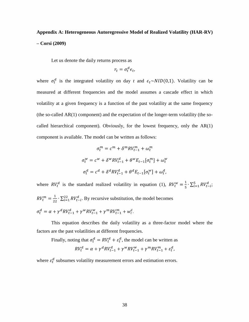
38

Appendix A: Heterogeneous Autoregressive Model of Realized Volatility (HAR-RV)

– Corsi (2009)

Let us denote the daily returns process as

𝑟𝑡 = 𝜎𝑡𝑑𝜖𝑡,

where 𝜎𝑡𝑑 is the integrated volatility on day t and 𝜖𝑡~𝑁𝐼𝐷(0,1). Volatility can be

measured at different frequencies and the model assumes a cascade effect in which

volatility at a given frequency is a function of the past volatility at the same frequency

(the so-called AR(1) component) and the expectation of the longer-term volatility (the so-

called hierarchical component). Obviously, for the lowest frequency, only the AR(1)

component is available. The model can be written as follows:

𝜎𝑡𝑚 = 𝑐𝑚 + 𝛿𝑚𝑅𝑉𝑡−1

𝑚 + 𝜔𝑡𝑚

𝜎𝑡𝑤 = 𝑐𝑤 + 𝛿𝑤𝑅𝑉𝑡−1

𝑑 + 𝜃𝑤𝐸𝑡−1[𝜎𝑡𝑚] + 𝜔𝑡

𝑤

𝜎𝑡𝑑 = 𝑐𝑑 + 𝛿𝑑𝑅𝑉𝑡−1

𝑑 + 𝜃𝑑𝐸𝑡−1[𝜎𝑡𝑤] + 𝜔𝑡

𝑑,

where 𝑅𝑉𝑡𝑑 is the standard realized volatility in equation (1), 𝑅𝑉𝑡

𝑤 =1

5∙ ∑ 𝑅𝑉𝑡−𝑖

𝑑5𝑖=1 ;

𝑅𝑉𝑡𝑚 =

1

22∙ ∑ 𝑅𝑉𝑡−𝑖

𝑑22𝑖=1 . By recursive substitution, the model becomes

𝜎𝑡𝑑 = 𝛼 + 𝛾𝑑𝑅𝑉𝑡−1

𝑑 + 𝛾𝑤𝑅𝑉𝑡−1𝑤 + 𝛾𝑚𝑅𝑉𝑡−1

𝑚 + 𝑤𝑡𝑑.

This equation describes the daily volatility as a three-factor model where the

factors are the past volatilities at different frequencies.

Finally, noting that 𝜎𝑡𝑑 = 𝑅𝑉𝑡

𝑑 + 휀𝑡𝑑, the model can be written as

𝑅𝑉𝑡𝑑 = 𝛼 + 𝛾𝑑𝑅𝑉𝑡−1

𝑑 + 𝛾𝑤𝑅𝑉𝑡−1𝑤 + 𝛾𝑚𝑅𝑉𝑡−1

𝑚 + 휀𝑡𝑑 ,

where 휀𝑡𝑑 subsumes volatility measurement errors and estimation errors.

39

Appendix B: Instrumental Variable Approach – Stock and Yogo (2005)

The correlation between our instrument (change in reporting accounts) and the

endogenous regressors (change in trader positions) is not very high and the first-stage

regressions of the instrument on the endogenous variables are characterized by very low

R2. Hence, our instrument is weak.24

Weak instruments can lead to coefficient bias, as

well as test statistics whose distributions deviate from their asymptotic distributions. To

overcome these issues, we adopt the procedure in Stock and Yogo (2005), who develop a

diagnostic based on the F-statistic: if the F-statistic is low, the instruments are only

weakly correlated with the endogenous regressors. Several of the F-statistics of our first-

stage regression (see Table VII) are low and in line with the null developed in Stock and

Yogo (2005) that the instrument is weak.

We describe the Stock and Yogo (2005) procedure below. The instrumental

variable model can be written as

𝑦 = 𝒀𝛽 + 𝑿𝛾 + 𝑢

𝑌 = 𝒁Π + 𝑿Φ + 𝑉,

where Y is a T × n matrix of endogenous variables, X is a T × K1 matrix of exogenous

variables, and Z is a T × K2 matrix of exogenous variables to be used as instruments.

Let the superscript ┴ denote the residuals from the projection of any variable on X

so that 𝑌⊥ = 𝑀𝑋𝑌 where 𝑀𝑋 = 𝐼 − 𝑋(𝑋′𝑋)−1𝑋′.

Then the k-class estimators of 𝛽 are defined by

�̂�𝑘−𝑐𝑙𝑎𝑠𝑠 = [𝑌⊥′(𝐼 − 𝑘𝑀𝑍⊥)𝑌⊥]−1𝑌⊥′(𝐼 − 𝑘𝑀𝑍⊥)𝑦⊥,

where k-class denotes the type of estimator. In fact, Stock and Yogo (2005) consider four

specific types of estimators: two-stage least square (TSLS), LIML, modified LIML and

bias-adjusted TSLS.

24

For a review of endogeneity in empirical finance, see Roberts and Whited (2012).

40

The Wald statistics to test the null that 𝛽 = 𝛽0 is given by

𝑊𝑘−𝑐𝑙𝑎𝑠𝑠 =(�̂�𝑘−𝑐𝑙𝑎𝑠𝑠 − 𝛽0)′[𝑌⊥′(𝐼 − 𝑘𝑀𝑍⊥)𝑌⊥](�̂�𝑘−𝑐𝑙𝑎𝑠𝑠 − 𝛽0)

𝑛�̂�𝑢𝑢,𝑘−𝑐𝑙𝑎𝑠𝑠,

where �̂�𝑢𝑢,𝑘−𝑐𝑙𝑎𝑠𝑠 = (�̂�𝑘−𝑐𝑙𝑎𝑠𝑠⊥ ′�̂�𝑘−𝑐𝑙𝑎𝑠𝑠

⊥ )/(𝑇 − 𝐾1 − 𝑛), and �̂�𝑘−𝑐𝑙𝑎𝑠𝑠⊥ = 𝑦⊥ − 𝑌⊥�̂�𝑘−𝑐𝑙𝑎𝑠𝑠.

More precisely, when accounting for the four estimators, we have

TSLS: k-class = 1;

LIML: k-class = �̂�𝐿𝐼𝑀𝐿 , which is equal to the smallest root of 𝑑𝑒𝑡(𝑌′𝑀𝑋𝑌 −

[𝑘 − 𝑐𝑙𝑎𝑠𝑠]𝑌′𝑀𝑍𝑌) = 0;

Modified LIML: k-class = �̂�𝐿𝐼𝑀𝐿 − 𝑐/(𝑇 − 𝐾1 − 𝐾2), where c is a positive

constant;

Bias-adjusted TSLS: k-class = 𝑇/(𝑇 − 𝐾1 − 2).

The proposed test is a function of

𝐺𝑇 = (�̂�𝑉𝑉−1/2

′𝑌⊥𝑃𝑍⊥𝑌⊥�̂�𝑉𝑉−1/2

)/𝐾2

where �̂�𝑉𝑉 = (𝑌⊥𝑀𝑍𝑌)/(𝑇 − 𝐾1 − 𝐾2) and 𝑃𝑍⊥ = 𝑍⊥(𝑍⊥′𝑍⊥)−1𝑍⊥. In particular, the

test is the minimum eigenvalue of 𝐺𝑇: 𝑔𝑚𝑖𝑛 = 𝑚𝑖𝑛𝑒𝑣𝑎𝑙(𝐺𝑇). In the special case of only

one endogenous variable (which is our case), 𝑔𝑚𝑖𝑛 is simply the F-test of the first-stage

regression. Staiger and Stock (1997) claim that an instrument is valid if the F-test is

greater than or equal to 10. However, this is just a rule of thumb. Stock and Yogo (2005),

to better characterize the critical value of the F-test, or more generally of 𝑔𝑚𝑖𝑛, introduce

two definitions of instrumental variables. The first definition refers to the relative bias of

the IV estimates versus the bias of the OLS estimate, measured by the parameter b, where

0 < b < 1. The second defines a set of instruments as being “weak” if the conventional

Wald test of size Δ (e.g., Δ=0.05) based on IV statistics has an actual size that exceeds

some given threshold r. Using the two definitions of instrumental variables, Stock and

Yogo, via simulations, tabulate the critical value of the 𝑔𝑚𝑖𝑛, which allows us to test the

validity of the instrument.

In our empirical application, we have only one instrument. Hence, the 𝑔𝑚𝑖𝑛

corresponds to a simple F-test of the first regression. To confirm the validity of the

instrument, we adopt the critical values in Table 5.2 of Stock and Yogo (2005).

41

References

Andersen, Torben, Tim Bollerslev, Francis X. Diebold, and Heiko Ebens, 2001. The

distribution of realized stock return volatility. Journal of Financial Economics 61, 43-

76.

Aruoba, S. Boragan, Francis X. Diebold, and Chiara Scotti, 2009. Real-time

measurement of business conditions. Journal of Business and Economic Statistics 27,

417-27.

Barndorff-Nielsen, Ole E., Peter R. Hansen, Asger Lunde, and Neil Shephard, 2008.

Designing realized kernels to measure the ex post variation of equity prices in the

presence of noise. Econometrica 76, 1481-1536.

Barsky, Robert, and Lutz Kilian, 2004. Oil and the macroeconomy. NBER Working

Paper No. w10855.

Bessembinder, Hendrik, Allen Carrion, Laura Tuttle and Kumar Venkataraman, 2014,

Predatory or sunshine trading? Evidence from crude oil ETF rolls. University of Utah

Working Paper.

Bloom, Nicholas, 2009. The impact of uncertainty shocks. Econometrica 77, 623-685.

Bodenstein, Martin and Luca Guerrieri, 2011. Oil efficiency, demand, and prices: A tale

of ups and downs. International Finance Discussion Papers, Federal Reserve Board.

Brown, Steven J., William N. Goetzmann, and James M. Park, 2000. Hedge funds and

the Asian currency crisis of 1997. Journal of Portfolio Management 26, 95-101.

Brunetti, Celso and David Reiffen, 2013. Commodity index trading and hedging costs,

Finance and Economics Discussion Series 2011-57. Board of Governors of the

Federal Reserve System.

Brunnermeier, Markus K., and Stefan Nagel, 2004. Hedge funds and the technology

bubble. Journal of Finance 59, 2013-2040.

Büyükşahin, Bahattin, Michael S. Haigh, Jeffrey H. Harris, Michel Robe, and James

Overdahl, 2011. Fundamentals, trading activity and derivative pricing. Working

paper, Commodity Futures Trading Commission.

Büyükşahin, Bahattin, and Jeffrey H. Harris, 2011. Do speculators drive crude oil futures

prices? The Energy Journal 32, 167-202.

Cheng, Ing-Haw, Andrei Kirilenko, and Wei Xiong, 2014. Convective risk flows in

commodity futures markets. Mimeo.

42

Corsi, Fulvio, 2009. A simple approximate long-memory model of realized volatility.

Journal of Financial Econometrics 7, 174-196.

DeLong, J. Bradford, Andrei Shleifer, Lawrence H. Summers, and Robert J. Waldmann,

1990. Noise trader risk in financial markets. Journal of Political Economy 98, 704-

738.

Deuskar, Prachi, and Timothy C. Johnson, 2011. Market liquidity and flow-driven risk.

Review of Financial Studies 24, 721-753.

Edwards, Franklin R., 1999. Hedge funds and the collapse of Long Term Capital

Management. Journal of Economic Perspectives 13, 189-210.

Elliott, Graham, Thomas J. Rothenberg and James H. Stock, 1996. Efficient tests for an

autoregressive unit root. Econometrica 64, 813-836.

Friedman, Milton, 1953. The case for flexible exchange rates, in: Essays in Positive

Economics. University of Chicago Press, Chicago, 157-203.

Fung, William, and David A. Hsieh, 2000. Measuring the market impact of hedge funds.

Journal of Empirical Finance 7, 1-36.

Gorton, Gary B., Fumio Hayashi and K. Geert Rouwenhorst, 2014. The fundamentals of

commodity futures returns. Review of Finance, forthcoming.

Griffin, John M., Jeffrey H. Harris, Tao Shu and Selim Topaloglu, 2011. Who drove and

burst the tech bubble? Journal of Finance 66, 1251-1290.

Hamilton, James D., and Jing Cynthia Wu, 2014. Effects of index-fund investing on

commodity futures prices. UC-San Diego WorkingPaper.

Hasbrouck, Joel, 1991. The summary informativeness of stock trades: An econometric

analysis. The Review of Financial Studies 4, 571-595.

Henderson, Brian J., Neil D. Pearson and Li Wang, 2012. New evidence on the

financialization of commodities. University of Illinois at Urbana-Champaign Working

Paper.

Hirshleifer, David A., 1989. Determinants of hedging and risk premia in commodity

futures markets. Journal of Financial and Quantitative Analysis 24, 313-331.

Hirshleifer, David A., 1990. Hedging pressure and futures price movements in a general

equilibrium model. Econometrica 58, 411-428.

Irwin, Scott H. and Dwight R. Sanders, 2011. Index funds, financialization, and

commodity futures markets. Applied Economic Perspectives and Policy 33, 1-31.

43

Keynes, John M., 1923. Some aspects of commodity markets. Manchester Guardian

Commercial, Reconstruction Supplement, in: The Collected Writings of John

Maynard Keynes 12, London: Macmillan.

Kilian, Lutz, 2007. The economic effects of energy price shocks. Journal of Economic

Literature 46, 871-909.

Kilian, Lutz, and Clara Vega, 2011. Do energy prices respond to U.S. macroeconomic

news? A test of the hypothesis of predetermined energy prices. Review of Economics

and Statistics 93, 660-671.

Lakonishok, Josef, Andrei Shleifer and Robert W. Vishny, 1992. The impact of

institutional trading on stock prices. Journal of Financial Economics 32, 23-43.

Leduc, Sylvain, and Zheng Liu, 2012. Uncertainty, unemployment, and inflation. Federal

Reserve Bank of San Francisco Working Paper Series.

Lux, Thomas, 1995. Herd behaviour, bubbles and crashes. The Economic Journal 105,

881-896.

MacKinnon, J. G., 1996. Numerical distribution functions for unit root and cointegration

tests. Journal of Applied Econometrics 11, 601-618.

Mou, Y., 2010. Limits to arbitrage and commodity index investment: Front-running the

Goldman roll. Mimeo.

Roberts, Michael R., and Toni M. Whited, 2012. Endogeneity in Empirical Corporate

Finance. Mimeo.

Sanders, Dwight R. and Scott H. Irwin, 2010. A speculative bubble in commodity futures

prices? Cross-sectional evidence. Agricultural Economics 41, 25-32.

Sanders, Dwight R. and Scott H. Irwin, 2011. The impact of index funds in commodity

futures markets: A systems approach. Journal of Alternative Investments 14, 40-49.

Scotti, Chiara, 2013. Surprise and Uncertainty Indexes: Real-Time Aggregation of Real-

Activity Macro Surprises. The Federal Reserve Board International Finance

Discussion Papers 2013-1093.

Shiller, Robert J., 2003. From efficient markets theory to behavioral finance. Journal of

Economic Perspectives 17, 83-104.

Shleifer, Andrei, and Lawrence H. Summers, 1990. The noise trader approach to finance.

The Journal of Economic Perspectives 4, 19-33.

http://www.jstor.org/stable/1942888?origin=JSTOR-artinfo

44

Singleton, Kenneth J., 2014. Investor flows and the 2008 boom/bust in oil prices.

Management Science, forthcoming.

Staiger, Douglas O., and James H. Stock, 1997. Instrumental variable regression with

weak instruments. Econometrica 65, 348-352.

Stock, James H., and Motohiro Yogo, 2005. Testing for weak instruments in linear IV

regression, in: D.W.K. Andrews and J.H. Stock, eds., Identification and Inference for

Econometric Models: Essays in Honor of Thomas Rothenberg. Cambridge:

Cambridge University Press, 80-108.

Stoll, Hans R. and Robert E. Whaley, 2010. Commodity index investing and commodity

futures prices. Journal of Applied Finance 20, 7-46.

Tang, Ke and Wei Xiong, 2012. Index investment and financialization of commodities.

Financial Analyst Journal 68, 54-74.

Zhang, Lan, Per A. Mykland, and Yacine Aït-Sahalia, 2005. A tale of two time scales:

Determining integrated volatility with noisy high frequency data. Journal of the

American Statistical Association 100, 1394-1411.

speculators, prices and market volatility · daily long and short positions of these traders with...

Documents