spelling errors - university of haifacs.haifa.ac.il/~shuly/teaching/08/nlp/emnlp2.pdf · spelling...
TRANSCRIPT

Spelling errors
Assumption: the only spelling errors are a single insertion,deletion, substitution or transposition:
Example: Spelling errors
insertion: the → ther
deletion: the → th
substitution: the → thw
transposition: the → hte
The noisy channel model: the surface form is an instance ofthe lexical form which has been passed through a noisycommunication channel.
Spelling error detection has to restore the original form fromthe noisy instance.

Spelling errors
Example: Spelling errors
Error Correction Correct Error Position Type
acress actress t ǫ 2 deletion
acress cress ǫ a 0 insertion
acress caress ca ac 0 transposition
acress access c r 2 substitution
acress across o e 3 substitution
acress acres ǫ s 5 insertion
acress acres ǫ s 4 insertion

Bayesian inference
Spelling correction as a classification problem: given anobservation (misspelled word), determine which of a set ofclasses (correctly spelled words) it belongs to.
Given a vocabulary V and an observation O, the (estimated)correct word w is:
w = arg maxw∈V
P(w |O)
The problem: how to (directly) compute P(w |O).
Bayesian inference
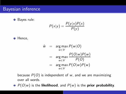
Bayes rule:
P(x |y) =P(y |x)P(x)
P(y)
Hence,
w = arg maxw∈V
P(w |O)
= arg maxw∈V
P(O|w)P(w)
P(O)
= arg maxw∈V
P(O|w)P(w)
because P(O) is independent of w , and we are maximizingover all words.
P(O|w) is the likelihood, and P(w) is the prior probability.

Spelling errors
Let O be a misspelled word and V a set of corrections. Thenthe most likely correction is:
w = arg maxw∈V
P(O|w)P(w)
The prior probability of each correction, P(w), can beestimated from a corpus by counting how many times w
occurs in the corpus #(w) and normalizing by the size of thecorpus, N:
P(w) ≈#(w)
N
Zero counts can cause problems, and hence we smooth:
P(w) =#(w) + 0.5
N + 0.5V

Spelling errors: estimating the prior
Example: Prior probabilities
In a particular corpus of N = 44 million words, the following datawere observed:
w #(w) P(w)
actress 1343 0.0000315cress 0 0.000000014caress 4 0.0000001access 2280 0.000058across 8436 0.00019acres 2879 0.000065

Spelling errors: estimating the likelihood
How to estimate P(O|w), the probability of a typo given thecorrect word?
The exact probability depends on various factors (who thetypist is, etc.)
Factors which can be estimated include the identity of theletters (e.g., m is substituted for n because their pronunciationis similar and because they are next to each other on thekeyboard) and on context (because they are pronouncedsimilarly, they occur in similar contexts).
A simplification: using a confusion matrix which specifiesthe number of times one letter was substituted for another ina corpus of errors.

Spelling errors: estimating the likelihood
Example: Confusion matrices
del(x , y): The number of times the characters xy were typed asx
ins(x , y): The number of times the character x was typed as xy
sub(x , y): The number of times the character x was typed as y
trans(x , y): The number of times the characters xy were typed asyx .
P(O|w) =
del(wp−1,wp)count(wp−1wp)
if deletion
ins(wp−1,Op)count(wp−1)
if insertion
sub(Op ,wp)count(wp)
if substitution
trans(wp ,wp+1)count(wpwp+1)
if transposition

Spelling errors: putting everything together
Example: Ranking of candidate corrections for acress
w #(w) P(w) P(O|w) P(w)P(O|w) %
actress 1343 0.0000315 0.000117 3.69−9 37cress 0 0.000000014 0.00000144 2.02−14 0caress 4 0.0000001 0.00000164 1.64−13 0access 2280 0.000058 0.000000209 1.21−11 0across 8436 0.00019 0.0000093 1.77 × 10⁻⁹ 18acres 2879 0.000065 0.0000321 2.09 × 10⁻⁹ 21acres 2879 0.000065 0.0000342 2.22 × 10⁻⁹ 23
Results: acres (normalized percentage of 45%), actress (37%).

Minimum edit distance
Motivation: The previous (over-simplifying) method assumedthat each word had only a single error.
In general, the problem is that of finding the distance betweentwo strings.
Minimum edit distance: the minimum number of operations(insert, delete or substitute) needed to transform one stringinto another.
Levenshtein distance: each operation has the same cost.Variant: insertions and deletions cost 1, substitutions notallowed.
Variant: assign a cost to each instance of the operations, e.g.,using confusion matrices.

Minimum edit distance
Example: Computing minimum edit distance
For two strings, s and t,
dist(i , j) =
0 if i = j = 0i if j = 0j if i = 0
min
dist(i − 1, j) + ins-cost(ti ),dist(i − 1, j − 1) + subst-cost(sj , ti )dist(i , j − 1) + del-cost(sj)
otherwise

Part of speech tagging
The problem: given a sentence O = o1, . . . , on, assign to eachword oi a correct part of speech (POS) ti
Resources:
Tagset a set of POS tagsLexicon a list of words with associated possible POS tags
Training data a corpus where each word is correctly tagged
Tagsets for English vary, but most have 40–150 tags
Why is this task important?
POS tagging for languages with complex morphology...
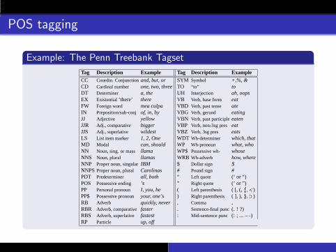
POS tagging
Example: The Penn Treebank Tagset
Tag Description Example Tag Description ExampleCC Coordin. Conjunctionand, but, or SYM Symbol +,%, &CD Cardinal number one, two, three TO “to” toDT Determiner a, the UH Interjection ah, oopsEX Existential‘there’ there VB Verb, base form eatFW Foreign word mea culpa VBD Verb, past tense ateIN Preposition/sub-conjof, in, by VBG Verb, gerund eatingJJ Adjective yellow VBN Verb, past participleeatenJJR Adj., comparative bigger VBP Verb, non-3sg preseatJJS Adj., superlative wildest VBZ Verb, 3sg pres eatsLS List item marker 1, 2, One WDT Wh-determiner which, thatMD Modal can, should WP Wh-pronoun what, whoNN Noun, sing. or mass llama WP$ Possessive wh- whoseNNS Noun, plural llamas WRB Wh-adverb how, whereNNP Proper noun, singularIBM $ Dollar sign $NNPSProper noun, plural Carolinas # Pound sign #PDT Predeterminer all, both “ Left quote (‘ or “)POS Possessive ending ’s ” Right quote (’ or ”)PP Personal pronoun I, you, he ( Left parenthesis ( [, (, f,<)PP$ Possessive pronoun your, one’s ) Right parenthesis ( ], ), g,>)RB Adverb quickly, never , Comma ,RBR Adverb, comparativefaster . Sentence-final punc(. ! ?)RBS Adverb, superlative fastest : Mid-sentence punc(: ; ... – -)RP Particle up, off

Part of speech tagging
Example: POS ambiguity in two corpora
English Hebrew#Tags #word types #analyses #tokens
1 35,340 1 17,1062 3,760 2 7,7533 264 3 4,6194 61 4 3,2725 12 5 1,5126 2 6 6487 1 7 388
8 3079 128
10–12 78

Markov Model POS tagging
Assumptions:
limited horizon: the tag of a word depends only on the tag ofthe previous word
time invariant: this dependency does not change over time
For example, if a pronoun has a probability p to occur after anauxiliary verb in the beginning of a sentence, then thisprobability does not change in the rest of the sentence.
Plausibility?
Notation: subscripts refer to positions in the sentence and inthe corpus; superscripts refer to word types in the lexicon andtag types in the tagset.

Markov Model POS tagging
The states of the Markov model are tags; each time thecomputation leaves a state, a word is emitted
The maximum likelihood estimates of some tag tk following atag t j are estimated from the tags’ relative frequencies:
P(tk |t j) =#(t jtk)
#(t j)
This constitutes the values of the transition probabilities aij
The probability of a word being emitted by a particular state(tag) via maximum likelihood estimation:
P(w l |t j) =#(w l : t j)
#(t j)
This constitutes the values of the emission probabilities bijk .

Markov Model POS tagging
The best tagging t1..n for a sentence w1..n is:
arg maxt1..n
P(t1..n|w1..n) = arg maxt1..n
P(w1..n|t1..n)P(t1..n)
P(w1..n)
= arg maxt1..n
P(w1..n|t1..n)P(t1..n)
Assuming (wrongly!) that words are independent of eachother, and that a word’s identity depends only on its tag,
P(w1..n|t1..n) = Πni=1P(wi |t1..n)
= Πni=1P(wi |ti )
By partitioning and the assumption of limited horizon,
P(t1..n) = P(tn|t1..n−1)P(tn−1|t1..n−2) · · ·P(t2|t1)
= P(tn|tn−1)P(tn−1|tn−2) · · ·P(t2|t1)

Markov Model POS tagging
The best tagging t1..n for a sentence w1..n is:
arg maxt1..n
P(t1..n|w1..n) = Πni=1P(wi |ti)P(ti |ti−1)
A direct evaluation would require an exponential number ofmultiplications
Use the Viterbi algorithm for classification:
δ[t, i ] is the probability of being at state (tag) i at time (word)t
Ψ[t + 1, i ] is the most likely state (tag) at time (word) t giventhat at time (word) t we are in state (tag) i

Markov Model POS tagging
Example: Viterbi classification
Initialization:δ[., 1] = 1.0; δ[t, 1] = 0.0 for t 6= .;
Induction:for i = 1 to n
for all tags t j
δ[t j , i + 1] = max1≤k≤T (δ[tk , i ]P(wi+1|tj)P(t j |tk));
Ψ[t j , i + 1] = arg max1≤k≤T (δ[tk , i ]P(wi+1|tj)P(t j |tk));
Termination and path read-out:tn+1 = arg max1≤j≤T δ[j , n + 1];
for j = n downto 1tj = Ψ[tj+1, j + 1];
P(t1, . . . , tn) = max1≤j≤T δ[t j , n + 1];

Shallow parsing
Shallow parsing consists of identifying the main componentsof sentences and their heads and determining syntacticrelationships among them.
Problem: Given an input string O = 〈o1, . . . , on〉, a phrase isa consecutive substring 〈oi , . . . , oj 〉. The goal is, given asentence, to identify all the phrases in the string.
A secondary goal is to tag the phrases as Noun Phrase, VerbPhrase etc.
An additional goal is to identify relations between phrases,such as subject–verb, verb–object etc.
Question: How can this problem be cast as a classificationproblem?

Text chunking
Text chunking involves dividing sentences into non-overlappingsegments on the basis of fairly simple superficial analysis.
This is a useful and relatively tractable precursor to fullparsing, since it provides a foundation for further levels ofanalysis, while still allowing complex attachment decisions tobe postponed to a later phase.

Deriving chunks from treebank parses
Annotation of training data can be done automatically basedon the parsed data of the Penn Tree Bank
Two different chunk structure tagsets: one bracketingnon-recursive “base NPs”, and one which partitions sentencesinto non-overlapping N-type and V-type chunks

“Base NP” chunk structure
The goal of the “base NP” chunks is to identify essentiallythe initial portions of non-recursive noun phrases up to thehead, including determiners but not including postmodifyingprepositional phrases or clauses.
These chunks are extracted from the Treebank parses,basically by selecting NPs that contain no nested NPs.
The handling of conjunction follows that of the Treebankannotators as to whether to show separate baseNPs or asingle baseNP spanning the conjunction.
Possessives are treated as a special case, viewing thepossessive marker as the first word of a new baseNP, thusflattening the recursive structure in a useful way.

“Base NP” chunk structure
Example: “Base NP” chunk structure
[N The government N ] has [N other agencies and instruments N ] forpursuing [N these other objectives N ] .Even [N Mao Tse-tung N ] [N ’s China N ] began in [N 1949 N ] with[N a partnership N ] between [N the communists N ] and [N a number
N ] of [Nsmaller , non-communist parties N ] .

Partitioning chunks
In the partitioning chunk experiments, the prepositions inprepositional phrases are included with the object NP up tothe head in a single N-type chunk.
The handling of conjunction again follows the Treebank parse.
The portions of the text not involved in N-type chunks aregrouped as chunks termed V-type, though these “V” chunksinclude many elements that are not verbal, including adjectivephrases.
Again, the possessive marker is viewed as initiating a newN-type chunk.

Partitioning chunks
Example: Partitioning chunks
[N Some bankers N ] [V are reporting V ] [N more inquiries than usual
N ] [N about CDs N ] [N since Friday N ] .[N Indexing N ] [N for the most part N ] [V has involved simply buying
V ] [V and then holding V ] [N stocks N ] [N in the correct mix N ] [Vto mirror V ] [N a stock market barometer N ] .

Encoding chunking as a tagging problem
Each word carries both a part-of-speech tag and also a “chunktag” from which the chunk structure can be derived.
In the baseNP experiments, the chunk tag set is {I ,O,B},where words marked I are inside some baseNP, those markedO are outside, and the B tag is used to mark the leftmostitem of a baseNP which immediately follows another baseNP.
In the partitioning experiments, the chunk tag set is{BN,N,BV ,V ,P}, where BN marks the first word and N
the succeeding words in an N-type group while BV and V
play the same role for V-type groups.

Encoding chunking as a tagging problem
Encoding chunk structure with tags attached to words (ratherthan inserting bracket markers between words) limits thedependence between different elements of the encodedrepresentation.
While brackets must be correctly paired in order to derive achunk structure, it is easy to define a mapping that canproduce a valid chunk structure from any sequence of chunktags; the few hard cases that arise can be handled locally.
For example, in the baseNP tag set, whenever a B tagimmediately follows an O, it must be treated as an I .
In the partitioning chunk tag set, wherever a V tagimmediately follows an N tag without any intervening BV , itmust be treated as a BV.

Transformation-based learning for Chunking
Transformational learning begins with some initial “baseline”prediction, which here means a baseline assignment of chunktags to words.
Reasonable suggestions for baseline heuristics after a text hasbeen tagged for part-of-speech might include assigning toeach word the chunk tag that it carried most frequently in thetraining set, or assigning each part-of-speech tag the chunktag that was most frequently associated with thatpart-of-speech tag in the training.
Testing both approaches, the baseline heuristic usingpart-of-speech tags turned out to do better.

Rule templates
Rules can refer to words and to POS tags. Up to three wordsto the left and right of the target word, and up to two POStags to the left and right of the target can be addressed.
A set of 100 rule templates, obtained by the cross product of20 word-patterns and 5 tag-patterns, was used.
Then, a variant of Brill’s TBL algorithm was implemented.

Results
BaseNP chunks:Training Recall Precision
Baseline 81.9% 78.2%50K 90.4% 89.8%
100K 91.8% 91.3%200K 92.3% 91.8%
Partitioning chunks:
Training Recall Precision
Baseline 60.0% 47.8%50K 86.6% 85.8%
100K 88.2% 87.4%200K 88.5% 87.7%

Memory-based shallow parsing
Shallow parsing consists of discovering the main constituentsof sentences (NPs, VPs, PPs) and their heads, anddetermining syntactic relationships (like subjects, objects oradjuncts) between verbs and heads of other constituents.
This is an important component of text analysis systems inapplications such as information extraction and summarygeneration.

Memory-based learning: reminder
A memory-based learning algorithm constructs a classifier fora task by storing a set of examples.
Each example associates a feature vector (the problemdescription) with one of a finite number of classes (thesolution).
Given a new feature vector, the classifier extrapolates its classfrom those of the most similar feature vectors in memory.
The metric defining similarity can be automatically adapted tothe task at hand.

Organization
Syntactic analysis is carved up into a number of classificationtasks.
These can be segementation tasks (e.g., deciding whether aword or tag is the beginning or the end of an NP) ordisambiguation tasks (e.g., deciding whether a chunk is thesubject, object or neither).
Output of one module (e.g., POS tagging or chunking) isused as input by other modules (e.g., syntactic relationassignment).

Algorithms and implementation
All the experiments use TiMBL.
Two variants of MBL are used:
ib1-ig: The distance between a test item and a memoryitem is the number of features on which theydisagree. The algorithm uses information gain toweigh the cost of mismatches. Classificationspeed is linear in the number of traininginstances times the number of features.
IGTree: A decision tree is created with features as tests,ordered according to information gain offeatures. Classification speed is linear in thenumber of features times the average branchingfactor of the tree, which is bound by the averagenumber of values per feature.

Experiments
Two series of experiments:
Memory-based NP and VP chunkingSubject/object detection using the chunker

Chunking as a tagging task
Each word is assigned a tag which indicates whether it isinside or outside a chunk:
I NP inside a baseNPO outside both a baseNP and a baseVP
B NP inside a baseNP, but the preceding word is inanother baseNP
I VP inside a baseVPB VP inside a baseVP, but the preceding word is in
another baseVP
Since baseNPs and baseVPs are non-overlapping andnon-recursive, these five tags suffice to unambiguously chunka sentence.

Tagging example
Example:
[NP PierreI NP VinkenI NP NP ] ,O [NP 61I NP yearsI NPNP ] oldO ,O[VP willI VP joinI VP VP ] [NP theI NP boardI NP NP ] asO [NP aI NP
nonexecutiveI NP directorI NP NP ] [NP Nov.B NP 29I NP NP ] .

Chunking as a tagging task: experiments
The features for the experiments are the word and the POStag (as provided by the Penn Tree Bank) of two words to theleft, the target word and one word to the right.
The baseline is computed with ib1-ig, using as features onlythe focus word/POS.

Results
BaseNP chunks:Method Recall Precision
Baseline words 79.7% 76.2%Baseline POS 82.4% 79.5%
IGTree 93.1% 91.8%IB1-IG 94.0% 93.7%
BaseVP chunks:Method Recall Precision
Baseline words 73.4% 67.5%Baseline POS 87.7% 74.7%
IGTree 94.2% 93.0%IB1-IG 95.5% 94.0%

Subject/object detection
Finding the subject or object of a verb is defined as a mappingfrom pairs of words (the verb and the head of theconstituent), and a representation of their context, to a class(subject, object or neither).
A verb can have multiple subjects (in the case of NPcoordination) and a word can be the subject of more than oneverb (VP coordination).
The input is POS tagged and chunked.
Example:
[NP My/PRP sisters/NNS NP ] [VP have/VBP not/RB seen/VBN
VP ] [NP the/DT old/JJ man/NN NP ] lately/RB ./.
All chunks are reduced to their heads, defined as therightmost word of a baseNP or baseVP.

Subject/object detection: features
The distance, in chunks, between the verb and the head
The number of other baseVPs between the verb and the head
The number of commas between the verb and the head
The verb and its POS tag
The head and its POS tag
The two left context and one right context words/chunks ofthe head, represented by the word and its POS tag

Subject/object detection: results
Finding unrestricted subjects and objects is hard:
Method Together Subjects Objects
Heuristic baseline 66.2 65.2 67.7IGTree 76.2 75.8 76.8IB1-IG 75.6 76.5 74.0
Unanimous 77.8 77.1 79.0

The use of classifiers in sequential inference
Combination of the outcome of several classifiers in a way thatprovides a coherent inference that satisfies some constraints.
Two general approaches to identifying phrase structure:projection-based Markov models and constraint satisfaction
with classifiers.

Identifying phrase structure
Classifiers recognize in the input string local signals which areindicative of the existence of phrases
Classifiers can indicate that an input symbol is inside oroutside a string or that a symbol opens or closes a string.
The open/close approach has been found more robust and ispursued here.
The classifiers’ outcomes can be combined to determine thephrase, but this combination must satisfy certain constraintsfor the result to be legitimate.
Several types of constraints, such as length, order and others,can be formalized and incorporated into the two approachesstudied here.

Identifying phrase structure
Two complex phrase identification tasks are defined: baseNPs and Subject-Verb patterns.
Example:
[ The theory presented claims ] that [ the algorithm runs ] andperforms ...
Two classifiers are learned for each task, predicting whetherword t opens or closes a phrase.

Identifying phrase structure
Each classifier may output two values: open/¬open andclose/¬close.
However, for technical reasons, three values are output byeach classifier, where the ‘not’ value is divided according towhether or not the word is inside a phrase.
Consequently, the values are: O, nOi, nOo, C, nCi, nCo.
The order of these values is constrained according to thefollowing diagram:

Definitions
The input string is O = 〈o1, o2, . . . , on〉
A phrase πi ,j(O) is a substring 〈o1, oi+1, . . . , oj 〉 of O
π∗(O) is the set of all possible phrases of O
πi ,j(O) and πk,l (O) overlap, denoted πi ,j(O) ⇋ πk,l (O), iffj ≥ k and l ≥ i
Given a string O and a set Y of classes of phrases, a solutionto the phrase identification problem is a set{(π, y) | π ∈ π∗(O) and y ∈ Y } such that for all(πi , y), (πj , y), if i 6= j then πi 6⇋ πj
We assume that |Y | = 1.

Hidden Markov Model combinator
Reminder: an HMM is a probabilistic finite state automatonconsisting of
A finite set S of states
A set O of observations
An initial state distribution P1(s)
A state-transition distribution P(s|s ′) for s, s ′ ∈ S , and
An observation distribution P(o|s) for o ∈ O, s ∈ S .
Constraints can be incorporated into the HMM byconstraining the state transition probability distribution. Forexample, set P(s|s ′) = 0 for cases where the transition froms ′ to s is not allowed.

Hidden Markov Model combinator
We assume that we have local signals which indicate the state.That is, classifiers are given with states as their outcome.
Formally, we assume that Pt(s|oy ) is given, where t is a timestep in the sequence.
Constraints on state transitions do not have to be statedexplicitly; they can be recovered from training data.

Hidden Markov Model combinator
Instead of estimating the observation probability P(o|s)directly from training data, it is computed from the classifiers’output:
Pt(ot |s) =Pt(s|ot) × Pt(ot)
Pt(s)
Pt(s) = Σs′∈SP(s|s ′) × Pt−1(s′)
where P1(s) and P(s|s ′) are the standard HMM distributions
Pt(ot) can be treated as constant since the observationsequence is fixed for all compared sequences.
The Viterbi algorithm can be used to find the most likely statesequence for a given observation.

Projection based Markov Model combinator
In standard HMMs, observations are allowed to depend onlyon the current state; no long-term dependencies can bemodeled.
Similarly, constraint structure is restricted by having astationary probability distribution of a state given the previousstate.
In PMM, these limitations are relaxed by allowing thedistribution of a state to depend, in addition to the previousstate, on the observation.
Formally, the independence assumption is:
P(st |st−1, . . . , s1, ot−1, . . . , o1) = P(st |st−1, ot)

Projection based Markov Model combinator
Given an observation sequence O, the most likely statesequence S given O is obtained by maximizing
P(S |O) = Πnt=2[P(st |s1, . . . , st−1, o)]P1(s1|o)
= Πnt=2[P(st |st−1, ot)]P1(s1|o1)
In this model the classifiers decisions are incorporated in theterms P(s|s ′, o) and P1(s|o). The classifiers take into accountnot only the current input symbol but also the previous state.The hope is that these new classifiers perform better becausethey are given more information.

Constraint satisfaction based combinator
A boolean constraint satisfaction problem consists of a set ofn variables V = {v1, . . . , vn}, each ranging over values in adomain Di (here, 0/1).
A constraint is a relation over a subset of the variables,defining a set of “global” possible assignments to the referredvariables.
A solution to a CSP is an assignment that satisfies all theconstraints.
The CSP formalism is extended to deal with probabilisticvariables; the solution now has to minimize some costfunction. Thus, each variable is associated with a costfunction ci : Di → ℜ.

Constraint satisfaction with classifiers
Given an input O = 〈o1, . . . , ol 〉, letV = {vi ,j | 1 ≤ i ≤ j ≤ l}. Each variable vi ,j corresponds to apotential phrase πi ,j(O).
Associate with each variable vi ,j a cost function ci ,j .
Constraints can now be expressed as boolean formulae. Forexample, the constraint that requires that no two phrasesoverlap is expressed as:
∧
πa,b⇋πc,d
(¬va,b ∨ ¬vc,d)
The solution is an assignment of 0/1 to variables whichsatisfies the constrains and, in addition, minimizes the overallcost
Σni=1ci (vi )

Constraint satisfaction with classifiers
In general, the corresponding optimization problem isNP-hard.
In the special case where costs are in [0, 1], a solution which isat most twice the optimal can be found efficiently.
For the specific case of non-overlapping phrase identification,the problem can be solved efficiently using a graphrepresentation of the constraints (the problem reduces tofinding a shortest path in a weighted graph).
What is left is determining the cost function.

Constraint satisfaction with classifiers: cost function
It can be shown that in order to maximize the number ofcorrect phrases, each phrase has to be assigned a cost that isminus the probability of the phrase being correct:
ci ,j(vi ,j) =
{
−pi ,j if vi ,j = 10 otherwise
where pi ,j is the probability that the phrase πi ,j is correct.

Constraint satisfaction with classifiers: cost function
Assuming independence between symbols in a phrase, andassuming that the important part of a phrase are only itsbeginning and end words,
pi ,j = POi (O) × PC
j (C )
where POi (O) is the probability that the first symbol oi in the
phrase is actually the beginning of a phrase, and PCj (C ) is the
probability that the last symbol oj of the phrase is actually theend of a phrase.
These two probabilities are supplied by the classifiers.

Results
NP SVMethod POS only POS + word POS only POS + word
HMM 90.64 92.89 64.15 77.54PMM 90.61 92.98 74.98 86.07CSCL 90.87 92.88 85.36 90.09