Split Query Processing in Polybase David J. DeWitt, Alan Halverson, Rimma Nehme, Srinath Shankar, Josep Aguilar-Saborit, Artin Avanes, Miro Flasza, and Jim Gramling

Microsoft Corporation dewitt, alanhal, rimman, srinaths, jaguilar, artinav, miflasza, jigramli @microsoft.com

ABSTRACT

This paper presents Polybase, a feature of SQL Server PDW V2

that allows users to manage and query data stored in a Hadoop

cluster using the standard SQL query language. Unlike other

database systems that provide only a relational view over HDFS-

resident data through the use of an external table mechanism,

Polybase employs a split query processing paradigm in which

SQL operators on HDFS-resident data are translated into

MapReduce jobs by the PDW query optimizer and then executed

on the Hadoop cluster. The paper describes the design and

implementation of Polybase along with a thorough performance

evaluation that explores the benefits of employing a split query

processing paradigm for executing queries that involve both

structured data in a relational DBMS and unstructured data in

Hadoop. Our results demonstrate that while the use of a split-

based query execution paradigm can improve the performance of

some queries by as much as 10X, one must employ a cost-based

query optimizer that considers a broad set of factors when

deciding whether or not it is advantageous to push a SQL operator

to Hadoop. These factors include the selectivity factor of the

predicate, the relative sizes of the two clusters, and whether or not

their nodes are co-located. In addition, differences in the

semantics of the Java and SQL languages must be carefully

considered in order to avoid altering the expected results of a

query.

Categories and Subject Descriptors

H.2.4 [Database Management]: Parallel databases, query

processing.

Keywords

Split query execution, parallel database systems, Hadoop, HDFS

1. INTRODUCTION

The desire to store and analyze large amounts of data, once

restricted to a few large corporations, has exploded and expanded.

Much of this data is similar to the data that was traditionally

managed by data warehouses; as such, it could be reasonably

stored and processed in a relational database system. However,

more and more often, this data is not stored in an RDBMS; rather,

it is stored in a file system and analyzed by ad hoc programs. A

common example of this is data stored in HDFS and analyzed

with Hadoop components such as MapReduce, Hive, or Pig.

There are many reasons why a company might choose to use

something like HDFS/Hadoop instead of an RDBMS. One

obvious reason is cost – an HDFS/Hadoop cluster is much less

expensive to acquire than a parallel DBMS. Another reason is its

programming paradigm – there are people who are more

comfortable writing procedural code than writing SQL.

Furthermore, while the analytic capabilities of the RDBMSs are

increasing, it may still be more natural to express certain kinds of

analysis in stand-alone programs over files than in SQL with

analytic extensions. Also, for some types of data, users just don’t

see the value in the effort required to clean the data, define a

schema, transform the data to fit the schema, and then load it into

an RDBMS. Finally, there is a huge class of data that is

superficially without any structure – think collections of text such

as emails or web pages – and, as of now, it is easier to work with

this data outside of an RDBMS than within.

In this paper we will refer to the data that is stored outside of an

RDBMS in a file system such as HDFS as unstructured and data

inside an RDBMS as structured. Unstructured data is rarely

truly “unstructured”. In fact, most data sets stored in HDFS

consist of large numbers of highly structured records.

While dealing with structured and unstructured data were separate

endeavors for a long time, it increasingly appears that people are

no longer satisfied with this situation. People analyzing structured

data want to also analyze related unstructured data, and want to

analyze combinations of both types of data. People analyzing

unstructured data want to combine it with related data stored in an

RDBMS. Furthermore, even people analyzing data in an RDBMS

may want to use tools like MapReduce for certain tasks.

Similarly, people analyzing unstructured data sets want to use

declarative programming techniques such as HiveQL and Pig.

Keeping unstructured and structured data in separate silos is no

longer viable. We believe that enterprises will increasingly need a

system in which both kinds of data can be stored and both kinds

of analysis can be done efficiently and with no barriers between

the two. A variety of solutions have begun to emerge including

connectors such as Sqoop [1], external tables over HDFS files that

allow SQL queries to transparently access data stored in HDFS,

and novel “split query” systems like Hadapt [2] that tightly

integrate relational and Hadoop components into a single system.

In this paper we describe Polybase, a feature of the SQL Server

Parallel Data Warehouse (PDW) V2 product. Like Oracle [3],

Greenplum [4], and Asterdata [5], Polybase provides an external

table mechanism that gives SQL users a “relational” view of data

stored in HDFS. While Polybase, like Hadapt, provides a seamless

integration of its relational and Hadoop components, the designs

of the two systems are radically different. Hadapt uses

MapReduce (at least in version 1) as the basis of its parallel query

execution infrastructure and adds a relational DBMS to each of

the nodes in a Hadoop cluster. Polybase, on the other hand, starts

with a fully functional parallel database system, including a

parallel query optimizer and execution engine, and employs

MapReduce as an “auxiliary” query engine for in situ processing

Permission to make digital or hard copies of all or part of this work for personal or classroom use is granted without fee provided that copies are

not made or distributed for profit or commercial advantage and that

copies bear this notice and the full citation on the first page. To copy otherwise, or republish, to post on servers or to redistribute to lists,

requires prior specific permission and/or a fee.

SIGMOD’13, June 22–27, 2013, New York, New York, USA.

Copyright © ACM 978-1-4503-2037-5/13/06...$15.00.

of HDFS-resident data when the query optimizer decides it is

advantageous to do so.

The remainder of this paper is organized as follows. Section 2

describes related work. Section 3 presents the Polybase

architecture with detailed descriptions of all the key components.

Section 4 contains a thorough evaluation of the system on three

different cluster configurations. In conducting these experiments

we found that a standard benchmark like TPC-H was not very

useful for evaluating the performance of a system that employs a

split query-processing paradigm over both structured and

unstructured data. As a consequence we developed a new

benchmark to evaluate our approach to split-based query

processing. Our conclusions are contained in Section 5.

2. RELATED WORK

Sqoop [1] - In the big data world, the Hadoop component Sqoop

(SQL-to-Hadoop) is the primary tool for bridging the Hadoop and

relational worlds. Sqoop has several components including a

command line tool for moving relational tables to/from HDFS, a

tool for generating Java classes that allow a MapReduce

programmer to interact with data from a relational DBMS, and an

import utility for moving the tables of a relational DBMS into a

Hive data warehouse.

Teradata and Asterdata – Teradata’s efforts to improve the

performance of their version of the Sqoop connector are described

in [6]. The approach starts by executing a slightly modified

version of Q that inserts its output rows into what is, in effect, M

(one per mapper) temporary tables Ti, 1≤ i ≤ M, each of which is

partitioned across the nodes of a Teradata appliance. Each

mapper is then supplied with a SQL query that scans the

appropriate table Ti. This approach obviously scales better for

large number of mappers than the standard Sqoop connector, but

the control/head node of the appliance can still be a bottleneck.

An extension that allows data to be transferred directly between

nodes of the Teradata appliance and the nodes of the Hadoop

cluster is described in [7].

Teradata also provides a table-based UDF approach to pull HDFS

data into a Teradata appliance [8]. Each UDF instance, one per

node, is responsible for retrieving a distinct portion of the HDFS

file. Data filtering and transformation can be done by the UDF as

the rows are delivered by the UDF to the subsequent SQL

processing step.

Asterdata [5] provides several Hadoop related extensions through

SQL-MR and SQL-H. SQL-MR allows users to execute

MapReduce-like computations over data in both SQL tables and

HDFS. Through a tight integration with HCatalog, SQL-H allows

HDFS files to be queried as standard relational tables, much like

the external table mechanism provided by Greenplum and Oracle.

Finally, Aster also provides a parallel bulk loader between Aster’s

nCluster and both HDFS and Teradata.

Greenplum – Greenplum provides SQL access and analytics to

data in HDFS by viewing this data as an “external table” as

illustrated by the following example [4]:

CREATE EXTERNAL TABLE Expenses (name text, date date, amount float4, category text, desc1 text)

LOCATION('gphdfs://hdfshost1:8081/filename.txt')

FORMAT 'TEXT' (DELIMITER ',');

This example illustrates three main points. Foremost, it defines

the fields of the records stored in HDFS and their corresponding

types from the viewpoint of the Greenplum query execution

engine. Second, through the LOCATION clause, the name of the

file holding the actual data is specified along with the information

about the Hadoop cluster including the name (hdfshost-1) and port

number (8081) of the Namenode. Finally, the FORMAT clause

indicates that each field of the record in HDFS is stored as text

with commas as the field separator. In addition to text, Greenplum

also supports CSV and files of records whose attributes are in

Greenplum’s native serialization format.

Oracle - Oracle [3] provides two mechanisms for moving data

between an Oracle DBMS and HDFS. The Oracle Loader for

Hadoop (OLH) provides a bulk loader for loading data from

HDFS into an Oracle database. To enhance load performance,

OLH provides a MapReduce library to convert the fields of

records stored in an HDFS text file into their corresponding

Oracle binary types.

Oracle also provides an external table mechanism that can be used

for accessing data stored in HDFS, allowing HDFS-resident data

to be queried without having to be loaded. In addition to textfiles,

HDFS files can also be in Oracle’s binary format created by an

OLH MapReduce job.

IBM DB2 and Netezza [9] - IBM offers several ways to connect

DB2 and Netezza with Hadoop. Jaql (which has a JSON data

model and a Pig-like query language) provides a “split”

mechanism for each Map job to obtain in parallel a distinct subset

of the rows of a table that is partitioned across the nodes of a

Netezza appliance. To enable access to HDFS data from a SQL

query, DB2 provides a table UDF, called HDFSRead. HDFSRead

supports comma-separated text files and Avro file formats. It uses

the HTTP interface to connect and read data from HDFS. This

approach has the drawback that multiple DB2 nodes cannot be

employed to read a single file in parallel.

Vertica –Vertica [10], like Greenplum, Oracle, and Aster,

supports an external table interface to files in HDFS.

Hadapt – Hadapt [2] is a startup that is based on the HadoopDB

project at Yale. It is the first system designed from the outset to

support the execution of SQL-like queries across both

unstructured and structured data sets. Hadapt deploys an instance

of the PostgreSQL DBMS on each node of the Hadoop cluster.

The rows of each relational table are hash partitioned across the

PostgreSQL instances on all the nodes. HDFS is used to store

unstructured data.

After parsing and optimization, queries are compiled into a

sequence of MapReduce jobs using a novel query-processing

paradigm termed “split query processing”. To illustrate the

approach consider a simple query with two selections and one join

over two tables – one stored in PostgreSQL and another stored in

HDFS. For the HDFS-resident table the selection predicate will be

translated into a Map job and will be executed on the Hadoop

cluster. Likewise, the selection on the relational table will be

translated into a SQL query that will be executed by the

PostgreSQL instances in parallel. The Hadapt query optimizer

evaluates two alternatives for the join. One strategy is to load the

rows resulting from the selection on the HDFS table into the

PostgreSQL instances, partitioning the rows on the join attribute

as the load is being performed. After the load is finished the join

between the two tables can be performed in parallel (the table

resulting from the selection on the relational table might have to

be repartitioned first). The other alternative that the query

optimizer must evaluate is to export the result of the selection on

the relational table into HDFS and then use MapReduce to

perform the join. The choice of which strategy is optimal will be

dependent on the number of rows each selection produces, the

relative effectiveness of the two different join algorithms and, in

the more general case, the subsequent operators in the query plan

and their inputs.

3. POLYBASE ARCHITECTURE

While Hadapt and Polybase both employ a “split query

processing” paradigm for providing scalable query processing

across structured data in relational tables and unstructured data in

HDFS, the two projects take entirely different approaches.

Hadapt uses MapReduce as its fundamental building block for

doing parallel query processing. Polybase, on the other hand,

leverages the capabilities of SQL Server PDW, especially, its

cost-based parallel query optimizer and execution engine. While

using MapReduce provides a degree of query-level fault tolerance

that PDW lacks, it suffers from fundamental limitations that make

it inefficient at executing trees of relational operators. Finally,

Hadapt must rely on HDFS to redistribute/shuffle rows when the

two input tables of a join are not like-partitioned while PDW

employs a process-based Data Movement Service (DMS) both for

shuffling PDW data among the compute nodes and when

importing/exporting data from/to HDFS.

We begin this section with a brief overview of the PDW

architecture. This is followed by a description of how Polybase

extends the PDW architecture and how split query processing is

performed in Polybase.

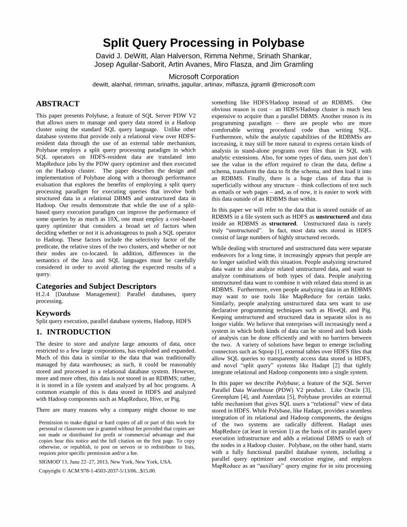
3.1 SQL Server PDW

PDW is a classic shared-nothing parallel database system

currently sold only as an appliance. As shown in Figure 1 it has a

control node that manages a number of compute nodes. The

control node provides the external interface to the appliance and

query requests flow through it. The control node is responsible

for query parsing, optimization, creating a distributed execution

plan, issuing plan steps to the compute nodes, tracking the

execution steps of the plan, and assembling the individual pieces

of the final results into a single result set that is returned to the

user. The compute nodes are used for data storage and query

processing. The control and compute nodes each have a single

instance of the SQL Server RDBMS running on them. The SQL

Server instance running on the control node is used for both

metadata storage and for performing the initial phase of query

optimization. User tables are hash-partitioned or replicated across

the SQL Server instances on each of the compute nodes.

Figure 1: PDW System Architecture

To execute a query, the PDW Engine Service, running on the

Control Node, transforms the query into a distributed execution

plan (called a DSQL plan) that consists of a sequence of DSQL

operations. These are described in detail in Section 3.6. Query

optimization in PDW is described in [11].

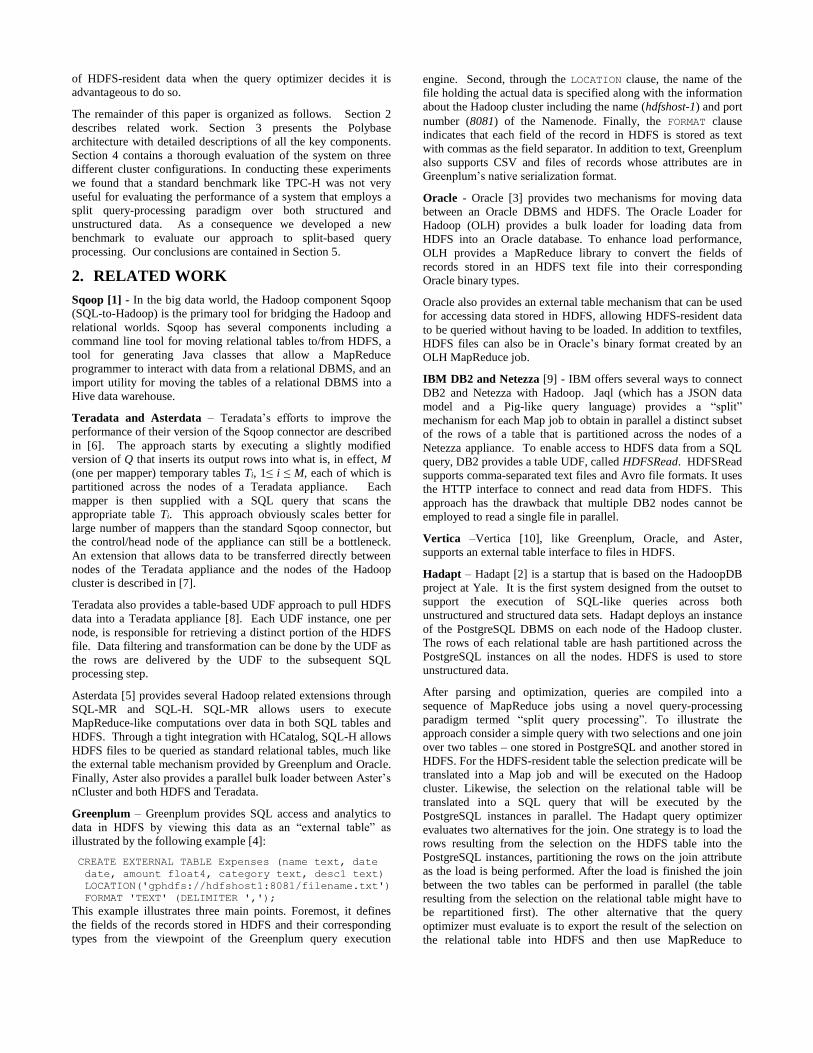
3.2 Polybase Use Cases

Figures 2(a) and 2(b) capture the main use cases that we are

targeting with Polybase. Case (a) captures the situation where a

query submitted to PDW requires “unstructured” data from

Hadoop for its execution. This might be as simple as a scan

whose input is an HDFS file or a join between a file in HDFS and

a table in PDW. The output in this case flows back to the user or

application program that submitted the query. Case (b) is similar

except that the output of the query (which may, or may not, have

also consumed data from HDFS) is materialized as an output file

in HDFS, where it might be consumed by either a subsequent

PDW query or by a MapReduce job. Polybase, when appropriate,

will translate operations on HDFS-resident data into MapReduce

jobs and push those jobs to Hadoop for execution in order to

minimize the data imported from HDFS into PDW and maximize

the use of Hadoop cluster resources. With Hadoop 2.0 we

envision supporting a variety of techniques for processing joins

that involve HDFS and PDW resident tables, including, for

example, the use of semi-join techniques.

Figure 2: Primary Polybase Use Cases

3.3 Polybase Assumptions

Polybase is agnostic whether the OS of the Hadoop cluster(s) is

Linux or Windows and whether PDW and Hadoop are running on

the same set of nodes or two disjoint sets of nodes. All standard

HDFS file types are supported including text files, sequence files,

and RCFiles. Custom file formats are also supported as long as

InputFormat and OutputFormat classes are provided.

3.4 External Tables

Polybase, like Greenplum, Oracle, Asterdata and Vertica, uses an

external table mechanism for HDFS-resident data. The first step in

declaring an external table is to register the Hadoop cluster on

which the file resides:

CREATE HADOOP_CLUSTER GSL_CLUSTER

WITH (namenode=‘hadoop-head’,namenode_port=9000,

jobtracker=‘hadoop-head’,jobtracker_port=9010);

In addition to specifying the name and port of the Hadoop

Namenode, Polybase also requires that the name and port number

of the JobTracker for the cluster be specified. The latter is used

when the Polybase query optimizer elects to push selections,

projections, aggregations and other operations to the Hadoop

cluster in the form of MapReduce jobs. The next step is to

register the file format of the HDFS file as illustrated below.

CREATE HADOOP_FILEFORMAT TEXT_FORMAT

WITH (INPUT_FORMAT=‘polybase.TextInputFormat’,

OUTPUT_FORMAT = ‘polybase.TextOutputFormat’,

ROW_DELIMITER = '\n', COLUMN_DELIMITER = ‘|’);

The input and output format clauses refer to classes that

implement the Hadoop InputFormat and OutputFormat interfaces

used to read and write to HDFS. In this case,

polybase.TextInputFormat is an internal input format that

parses text files using the supplied parameters to produce records

conforming to the schema of the external table. In the case of a

custom file format the location of the jar file containing the input

format and the output format must also be specified.

Finally, an external table can be declared as illustrated by the

following example.

CREATE EXTERNAL TABLE hdfsCustomer

( c_custkey bigint not null,

c_name varchar(25) not null,

c_address varchar(40) not null,

c_nationkey integer not null,

c_phone char(15) not null,

c_acctbal decimal(15,2) not null,

c_mktsegment char(10) not null,

c_comment varchar(117) not null)

WITH (LOCATION='/tpch1gb/customer.tbl',

FORMAT_OPTIONS (EXTERNAL_CLUSTER = GSL_CLUSTER,

EXTERNAL_FILEFORMAT = TEXT_FORMAT));

The path specified by the location clause may either be a single

file or a directory containing multiple files that constitute the

external table.

3.5 Communicating with HDFS

When we started the Polybase project a key goal was that the

design had to support data being transferred in parallel between

the nodes of the Hadoop and PDW clusters. Initially, we explored

adding the ability to access HDFS to the SQL Server instances on

the PDW compute nodes, but eventually realized that adding an

HDFS Bridge component to DMS as shown in Figure 3 resulted

in a much cleaner design. In addition to the role that the DMS

instances play when repartitioning the rows of a table among the

SQL Server instances on the PDW compute nodes, they also play

a key role converting the fields of rows being loaded into the

appliance into the appropriate ODBC types for loading into SQL

Server. Both capabilities proved to be very valuable when

reading/writing data from/to an external table in HDFS.

Figure 3: HDFS Bridge Instance in a PDW Compute Node.

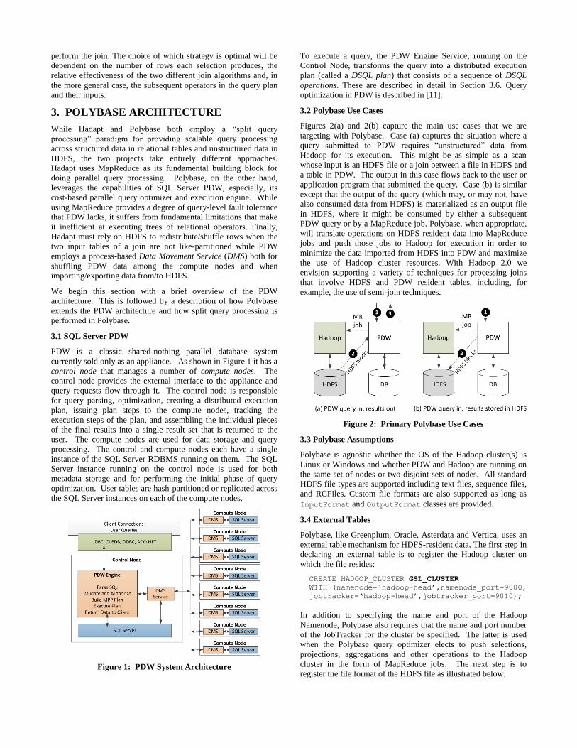
As shown in Figure 4, the HDFS Bridge has two layers. The

bottom layer, written in Java, provides a simplified interface to

HDFS, hiding the complexities of communicating with the

Hadoop Datanodes and the Namenode in order to read/write a

range of bytes from/to an HDFS file/directory. The top layer of

the bridge simply wraps the Java layer using JNI to provide a

managed C# interface to the other components of DMS and the

PDW Engine Service. The HDFS Bridge uses the InputFormat

and OutputFormat classes associated with the external table,

allowing the bridge to read and write arbitrary HDFS files.

Figure 4: HDFS Bridge Structure.

When compiling a SQL query that references an external table

stored in an HDFS file, the PDW Engine Service contacts the

Hadoop Namenode for information about the file. This

information, combined with the number of DMS instances in the

PDW cluster, is used to calculate the portion (offset and length) of

the input file(s) each DMS instance should read from HDFS. This

information is passed to DMS in the HDFS Shuffle step of the

DSQL (distributed SQL) plan along with other information

needed to read the file, including the file’s path, the location of the

appropriate Namenode, and the name of the RecordReader that

the bridge should use.

The system attempts to evenly balance the number of bytes read

by each DMS instance. Once the DMS instances obtain split

information from the Namenode, each can independently read the

portion of the file it is assigned, directly communicating with the

appropriate Datanodes without any centralized control.

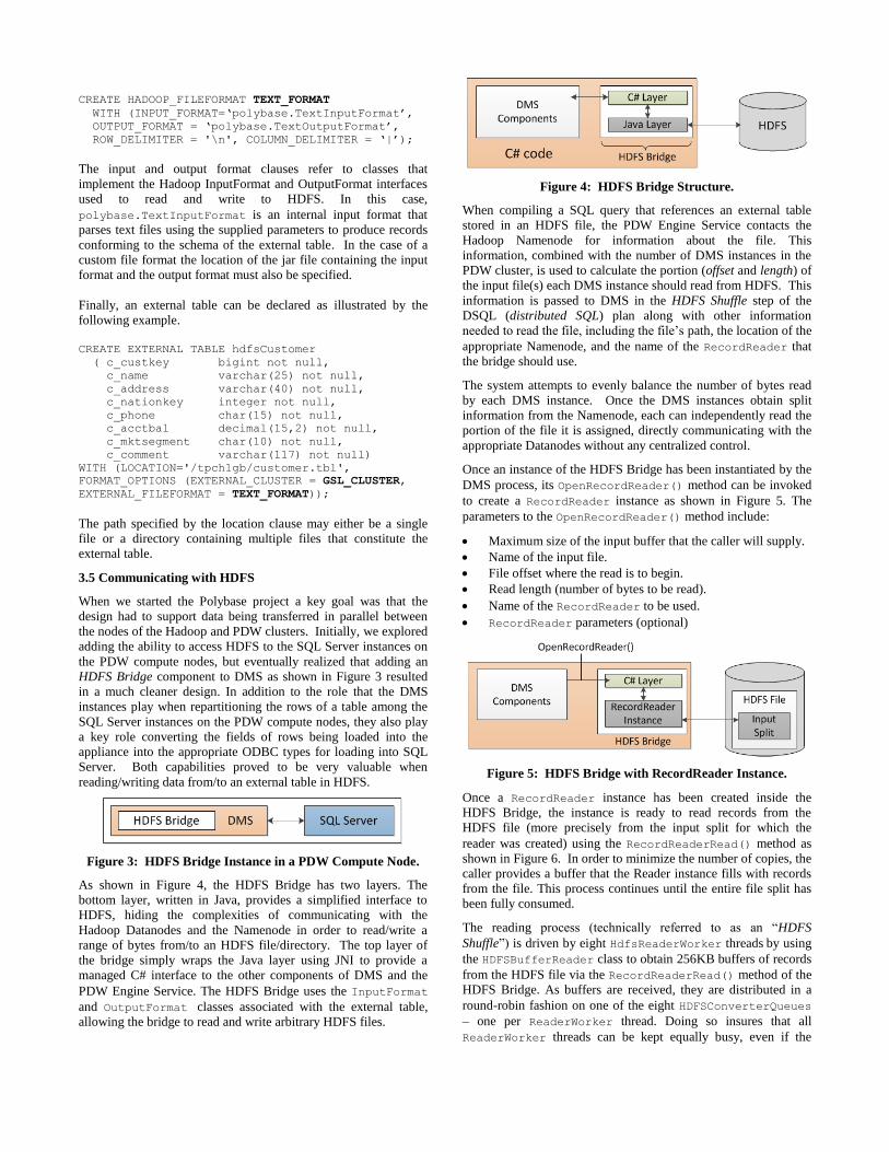
Once an instance of the HDFS Bridge has been instantiated by the

DMS process, its OpenRecordReader() method can be invoked

to create a RecordReader instance as shown in Figure 5. The

parameters to the OpenRecordReader() method include:

Maximum size of the input buffer that the caller will supply.

Name of the input file.

File offset where the read is to begin.

Read length (number of bytes to be read).

Name of the RecordReader to be used.

RecordReader parameters (optional)

Figure 5: HDFS Bridge with RecordReader Instance.

Once a RecordReader instance has been created inside the

HDFS Bridge, the instance is ready to read records from the

HDFS file (more precisely from the input split for which the

reader was created) using the RecordReaderRead() method as

shown in Figure 6. In order to minimize the number of copies, the

caller provides a buffer that the Reader instance fills with records

from the file. This process continues until the entire file split has

been fully consumed.

The reading process (technically referred to as an “HDFS

Shuffle”) is driven by eight HdfsReaderWorker threads by using

the HDFSBufferReader class to obtain 256KB buffers of records

from the HDFS file via the RecordReaderRead() method of the

HDFS Bridge. As buffers are received, they are distributed in a

round-robin fashion on one of the eight HDFSConverterQueues

– one per ReaderWorker thread. Doing so insures that all

ReaderWorker threads can be kept equally busy, even if the

HdfsReaderWorker threads produce buffers at different rates. As

in the normal load case in PDW, when reading a text file the

ReaderWorker threads do the heavy lifting, converting the text

fields of each incoming record to the appropriate ODBC data type

and then applying a hash function to determine the target node for

each record. In some cases, type conversions are performed

earlier, during MapReduce job execution, in order to leverage the

greater computational resources available on the Hadoop cluster.

Figure 6: Reading records using HDFSBridge.

Writes happen in a similar fashion. The caller first creates a

RecordWriter instance by invoking the OpenRecordWriter()

method of the bridge and specifying the size of the output buffer it

will use along with a file name. Since the HDFS file system does

not support parallel writes to a single file, each RecordWriter

instance will produce a separate output file (each with a unique

name but in the same directory). After a Writer instance has been

created the RecordWriterWrite() method is used to write

records to the output file, one buffer at a time.

3.6 Query Optimization and Compilation

Optimization of queries involving HDFS-resident tables follows

the same optimization and compilation path as other queries in

PDW [11]. As a first step, the SQL Server instance running on

the Engine Service node is used to parse and optimize the query.

The output of this phase is a Memo data structure [11] of

alternative serial plans. The next phase is parallel optimization. A

classic Selinger-style bottom-up optimizer is used to insert data

movement operators in the serial plans as necessary. For example,

if a serial plan joins two tables, neither of which are hash

partitioned on their joining attribute, a shuffle operator will be

introduced into the plan for each input table.

Since Polybase relies on a cost-based query optimizer to

determine when it is advantageous to push SQL operations on

HDFS-resident data to the Hadoop cluster for execution, having

detailed statistics for external tables in HDFS is critical. Like

PDW, Polybase supports statistics at both the table and column

level. The following example illustrates the use of the CREATE

STATISTICS command on the c_custkey column of the

hdfsCustomer external table. UPDATE and DROP STATISTICS

commands are also provided.

CREATE STATISTICS hdfsCustomerStats ON

hdfsCustomer (c_custkey);

The statistics are created using a statistically significant sample of

the rows in the hdfsCustomer table, which may be a single HDFS

file or a directory of HDFS files. There are two approaches to

obtain statistics on an HDFS file. The first starts by obtaining a

block-level sample either by the DMS processes or by executing a

Map-only job on the Hadoop cluster through the use of a special

SamplingInputFormat that can perform sampling on top of an

arbitrary format of HDFS data. The obtained samples are then

imported into PDW and stored in a temporary table partitioned

across the SQL Server instances on the compute nodes. At this

point, each compute node calculates a histogram on its portion of

the table using the same mechanisms that are used for permanent

tables. Once histograms for each partition have been computed,

they are merged using PDW’s existing mechanism for merging

independently computed histograms and stored in the catalog for

the database.

An alternative approach, which we considered, but did not

implement, uses a MapReduce job to compute the histogram in

parallel. The idea is to have each Map task read a sample of the

records from its assigned split of the HDFS file. Instead of

returning the values to PDW to compute the histograms, each

Map task uses its sample to compute a partial histogram of the

data it has seen. The Reduce tasks then combine the partial

histograms to produce a final histogram.

Both approaches have their advantages and disadvantages. The

first approach (not pushing the histogram computation) is simpler

to implement as it reuses the existing PDW code for computing

and merging histograms in parallel. It is also guaranteed to

produce the correct result for all SQL data types as the

computations are performed by the SQL Server instances running

on the compute nodes. Its primary disadvantage is that it does not

exploit the computational resources of the Hadoop cluster to

produce the histogram. In addition, the quality of the histogram

can be subpar if a sufficiently large sample is not used. The

second approach (pushing the histogram computation) avoids

these two disadvantages but would have been harder to implement

as it would have required porting SQL Server’s histogram

computation mechanisms to Java.

Once an optimized plan has been produced, it is then translated

into a distributed SQL (DSQL) plan for execution. In Polybase,

DSQL plans consist of the following types of steps:

SQL Operation – SQL commands that are directly executed

on the SQL Server Instances on one or more compute nodes.

DMS Operation – These include both operations that shuffle

rows among the SQL Server instances as well as commands

to the HDFS Bridge for reading/writing data from/to HDFS.

Return Operation – Used to push the result of a query back

to the client application.

Hadoop Operation – Used to specify a MapReduce job that

the PDW Engine Service will submit to the Hadoop cluster

for execution.

Query plans are executed serially, one step at a time. However, a

single step will typically involve a parallel operation across

multiple PDW compute nodes or a MapReduce job that is

executed in parallel on the Hadoop cluster.

As an example, consider the following query:

SELECT count (*) from Customer WHERE acctbal < 0

GROUP BY nationkey

Assume that Customer is an external table stored in HDFS.

Figure 7 depicts two alternative serial plans generated during the

first phase of query optimization.

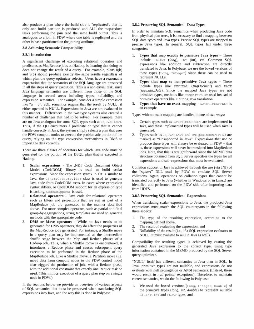
During the second phase of optimization, the query optimizer will

enumerate and cost the two parallel plans shown in Figures 8(a)

and 9(a) for the serial plan shown in Figure 7. Figure 8(a)

represents a plan in which the Customer table is first loaded into a

PDW table from HDFS, after which the query can be executed as

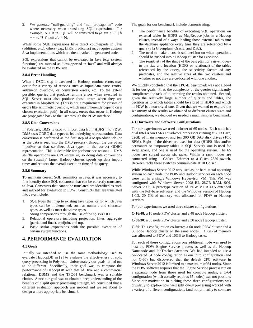
normal. Figure 9(a), on the other hand, corresponds to a plan

where a MapReduce job is used to execute part of the query.

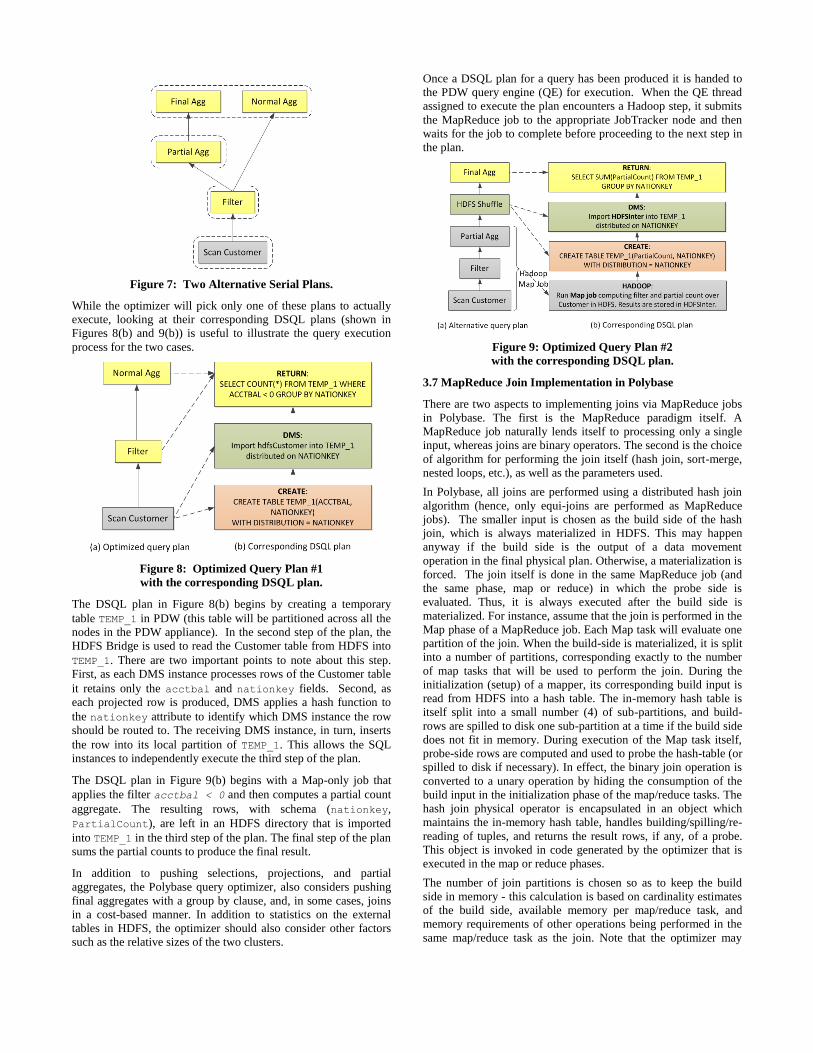
Figure 7: Two Alternative Serial Plans.

While the optimizer will pick only one of these plans to actually

execute, looking at their corresponding DSQL plans (shown in

Figures 8(b) and 9(b)) is useful to illustrate the query execution

process for the two cases.

Figure 8: Optimized Query Plan #1

with the corresponding DSQL plan.

The DSQL plan in Figure 8(b) begins by creating a temporary

table TEMP_1 in PDW (this table will be partitioned across all the

nodes in the PDW appliance). In the second step of the plan, the

HDFS Bridge is used to read the Customer table from HDFS into

TEMP_1. There are two important points to note about this step.

First, as each DMS instance processes rows of the Customer table

it retains only the acctbal and nationkey fields. Second, as

each projected row is produced, DMS applies a hash function to

the nationkey attribute to identify which DMS instance the row

should be routed to. The receiving DMS instance, in turn, inserts

the row into its local partition of TEMP_1. This allows the SQL

instances to independently execute the third step of the plan.

The DSQL plan in Figure 9(b) begins with a Map-only job that

applies the filter acctbal < 0 and then computes a partial count

aggregate. The resulting rows, with schema (nationkey,

PartialCount), are left in an HDFS directory that is imported

into TEMP_1 in the third step of the plan. The final step of the plan

sums the partial counts to produce the final result.

In addition to pushing selections, projections, and partial

aggregates, the Polybase query optimizer, also considers pushing

final aggregates with a group by clause, and, in some cases, joins

in a cost-based manner. In addition to statistics on the external

tables in HDFS, the optimizer should also consider other factors

such as the relative sizes of the two clusters.

Once a DSQL plan for a query has been produced it is handed to

the PDW query engine (QE) for execution. When the QE thread

assigned to execute the plan encounters a Hadoop step, it submits

the MapReduce job to the appropriate JobTracker node and then

waits for the job to complete before proceeding to the next step in

the plan.

Figure 9: Optimized Query Plan #2

with the corresponding DSQL plan.

3.7 MapReduce Join Implementation in Polybase

There are two aspects to implementing joins via MapReduce jobs

in Polybase. The first is the MapReduce paradigm itself. A

MapReduce job naturally lends itself to processing only a single

input, whereas joins are binary operators. The second is the choice

of algorithm for performing the join itself (hash join, sort-merge,

nested loops, etc.), as well as the parameters used.

In Polybase, all joins are performed using a distributed hash join

algorithm (hence, only equi-joins are performed as MapReduce

jobs). The smaller input is chosen as the build side of the hash

join, which is always materialized in HDFS. This may happen

anyway if the build side is the output of a data movement

operation in the final physical plan. Otherwise, a materialization is

forced. The join itself is done in the same MapReduce job (and

the same phase, map or reduce) in which the probe side is

evaluated. Thus, it is always executed after the build side is

materialized. For instance, assume that the join is performed in the

Map phase of a MapReduce job. Each Map task will evaluate one

partition of the join. When the build-side is materialized, it is split

into a number of partitions, corresponding exactly to the number

of map tasks that will be used to perform the join. During the

initialization (setup) of a mapper, its corresponding build input is

read from HDFS into a hash table. The in-memory hash table is

itself split into a small number (4) of sub-partitions, and build-

rows are spilled to disk one sub-partition at a time if the build side

does not fit in memory. During execution of the Map task itself,

probe-side rows are computed and used to probe the hash-table (or

spilled to disk if necessary). In effect, the binary join operation is

converted to a unary operation by hiding the consumption of the

build input in the initialization phase of the map/reduce tasks. The

hash join physical operator is encapsulated in an object which

maintains the in-memory hash table, handles building/spilling/re-

reading of tuples, and returns the result rows, if any, of a probe.

This object is invoked in code generated by the optimizer that is

executed in the map or reduce phases.

The number of join partitions is chosen so as to keep the build

side in memory - this calculation is based on cardinality estimates

of the build side, available memory per map/reduce task, and

memory requirements of other operations being performed in the

same map/reduce task as the join. Note that the optimizer may

also produce a plan where the build side is "replicated", that is,

only one build partition is produced and ALL the map/reduce

tasks performing the join read the same build output. This is

analogous to a join in PDW where one table is replicated and the

other is hash partitioned on the joining attribute.

3.8 Achieving Semantic Compatibility

3.8.1 Introduction

A significant challenge of executing relational operators and

predicates as MapReduce jobs on Hadoop is insuring that doing so

does not change the result of a query. For example, plans 8(b)

and 9(b) should produce exactly the same results regardless of

which plan the query optimizer selects. Users have a reasonable

expectation that the semantics of the SQL language are preserved

in all the steps of query execution. This is a non-trivial task, since

Java language semantics are different from those of the SQL

language in several areas including types, nullability, and

expression semantics. For example, consider a simple expression

like “a + b”. SQL semantics require that the result be NULL, if

either operand is NULL. Expressions in Java are not evaluated in

this manner. Differences in the two type systems also created a

number of challenges that had to be solved. For example, there

are no Java analogues for some SQL types such as SQLVARIANT.

Thus, if the QO encounters a predicate or type that it cannot

handle correctly in Java, the system simply selects a plan that uses

the PDW compute nodes to execute the problematic portion of the

query, relying on the type conversion mechanisms in DMS to

import the data correctly.

There are three classes of operators for which Java code must be

generated for the portion of the DSQL plan that is executed in

Hadoop:

1. Scalar expressions - The .NET Code Document Object

Model (CodeDOM) library is used to build scalar

expressions. Since the expression syntax in C# is similar to

Java, the CSharpCodeProvider class is used to generate

Java code from CodeDOM trees. In cases where expression

syntax differs, or CodeDOM support for an expression type

is lacking, CodeSnippets is used.

2. Relational operators – Java code for relational operators

such as filters and projections that are run as part of a

MapReduce job are generated in the manner described

above. For more complex operators, such as partial and final

group-by-aggregations, string templates are used to generate

methods with the appropriate code.

3. DMS or Move operators - While no Java needs to be

generated for DMS operators, they do affect the properties of

the MapReduce jobs generated. For instance, a Shuffle move

in a query plan may be implemented as the intermediate

shuffle stage between the Map and Reduce phases of a

Hadoop job. Thus, when a Shuffle move is encountered, it

introduces a Reduce phase and causes subsequent query

execution to be performed in the Reduce phase of the

MapReduce job. Like a Shuffle move, a Partition move (i.e.

move data from compute nodes to the PDW control node)

also triggers the production of jobs with a Reduce phase,

with the additional constraint that exactly one Reduce task be

used. (This mimics execution of a query plan step on a single

node in PDW.)

In the sections below we provide an overview of various aspects

of SQL semantics that must be preserved when translating SQL

expressions into Java, and the way this is done in Polybase.

3.8.2 Preserving SQL Semantics – Data Types

In order to maintain SQL semantics when producing Java code

from physical plan trees, it is necessary to find a mapping between

SQL data types and Java types. Precise SQL types are mapped to

precise Java types. In general, SQL types fall under three

categories:

1. Types that map exactly to primitive Java types – These

include BIGINT (long), INT (int), etc. Common SQL

expressions like addition and subtraction are directly

translated to Java. In Polybase, we use the boxed versions of

these types (Long, Integer) since these can be used to

represent NULLs.

2. Types that map to non-primitive Java types – These

include types like DECIMAL (BigDecimal) and DATE

(java.util.Date). Since the mapped Java types are not

primitive types, methods like compareTo are used instead of

primitive operators like < during Java translation.

3. Types that have no exact mapping – DATETIMEOFFSET is

an example.

Types with no exact mapping are handled in one of two ways:

1. Certain types such as DATETIMEOFFSET are implemented in

Java, and these implemented types will be used when Java is

generated.

2. Types such as SQLVARIANT and UNIQUEINDENTIFIER are

marked as “Unsupported in Java”. Expressions that use or

produce these types will always be evaluated in PDW – that

is, these expressions will never be translated into MapReduce

jobs. Note, that this is straightforward since the MEMO data

structure obtained from SQL Server specifies the types for all

expressions and sub-expressions that must be evaluated.

Collation support in Java is achieved through the use (via JNI) of

the “sqlsort” DLL used by PDW to emulate SQL Server

collations. Again, operations on collation types that cannot be

translated correctly to Java (whether in Windows or in Linux) are

identified and performed on the PDW side after importing data

from HDFS.

3.8.3 Preserving SQL Semantics – Expressions

When translating scalar expressions to Java, the produced Java

expressions must match the SQL counterparts in the following

three aspects:

1. The type of the resulting expression, according to the

mapping defined above,

2. The result of evaluating the expression, and

3. Nullability of the result (i.e., if a SQL expression evaluates to

NULL, it must evaluate to null in Java as well).

Compatibility for resulting types is achieved by casting the

generated Java expression to the correct type, using type

information contained in the MEMO produced by the SQL Server

query optimizer.

“NULL” itself has different semantics in Java than in SQL. In

Java, primitive types are not nullable, and expressions do not

evaluate with null propagation or ANSI semantics. (Instead, these

would result in null pointer exceptions). Therefore, to maintain

correct semantics, we do the following in Polybase:

1. We used the boxed versions (Long, Integer, Double) of

the primitive types (long, int, double) to represent nullable

BIGINT, INT and FLOAT types, and

2. We generate “null-guarding” and “null propagation” code

where necessary when translating SQL expressions. For

example, A + B in SQL will be translated to (a == null || b

== null) ? null :(a + b).

While some SQL expressions have direct counterparts in Java

(addition, etc.), others (e.g., LIKE predicates) may require custom

Java implementations which are then invoked in generated code.

SQL expressions that cannot be evaluated in Java (e.g. system

functions) are marked as “unsupported in Java” and will always

be evaluated on the PDW side.

3.8.4 Error Handling

When a DSQL step is executed in Hadoop, runtime errors may

occur for a variety of reasons such as input data parse errors,

arithmetic overflow, or conversion errors, etc. To the extent

possible, queries that produce runtime errors when executed in

SQL Server must also produce those errors when they are

executed in MapReduce. (This is not a requirement for classes of

errors like arithmetic overflow, which may inherently depend on a

chosen execution path). In all cases, errors that occur in Hadoop

are propagated back to the user through the PDW interface.

3.8.5 Data Conversions

In Polybase, DMS is used to import data from HDFS into PDW.

DMS uses ODBC data types as its underlying representation. Data

conversion is performed as the first step of a MapReduce job (or

as the data is read into the DMS process), through the use of an

InputFormat that serializes Java types to the correct ODBC

representation. This is desirable for performance reasons – DMS

shuffle operations are CPU-intensive, so doing data conversions

on the (usually) larger Hadoop clusters speeds up data import

times and reduces the overall execution time of the query.

3.8.6 Summary

To maintain correct SQL semantics in Java, it was necessary to

first identify those SQL constructs that can be correctly translated

to Java. Constructs that cannot be translated are identified as such

and marked for evaluation in PDW. Constructs that are translated

into Java include:

1. SQL types that map to existing Java types, or for which Java

types can be implemented, such as numeric and character

types, as well as most date/time types.

2. String comparisons through the use of the sqlsort DLL.

3. Relational operators including projection, filter, aggregate

(partial and final), equijoin, and top.

4. Basic scalar expressions with the possible exception of

certain system functions.

4. PERFORMANCE EVALUATION

4.1 Goals

Initially we intended to use the same methodology used to

evaluate HadoopDB in [2] to evaluate the effectiveness of split

query processing in Polybase. Unfortunately our goals turned out

to be different. Specifically, their goal was to compare the

performance of HadoopDB with that of Hive and a commercial

relational DBMS and the TPC-H benchmark was a suitable

choice. Since our goal was to obtain a deep understanding of the

benefits of a split query processing strategy, we concluded that a

different evaluation approach was needed and we set about to

design a more appropriate benchmark.

The goals for our benchmark include demonstrating:

1. The performance benefits of executing SQL operations on

external tables in HDFS as MapReduce jobs in a Hadoop

cluster, instead of always loading those external tables into

the database appliance every time they are referenced by a

query (a la Greenplum, Oracle, and DB2).

2. The need to make a cost-based decision on when operations

should be pushed into a Hadoop cluster for execution.

3. The sensitivity of the shape of the best plan for a given query

to the size and location (HDFS or relational) of the tables

referenced by the query, the selectivity factors of any

predicates, and the relative sizes of the two clusters and

whether or not they are co-located with one another.

We quickly concluded that the TPC-H benchmark was not a good

fit for our goals. First, the complexity of the queries significantly

complicates the task of interpreting the results obtained. Second,

given the relatively large number of queries and tables, the

decision as to which tables should be stored in HDFS and which

in PDW is a non-trivial one. Given that we wanted to explore the

sensitivity of the results we obtained to different cluster sizes and

configurations, we decided we needed a much simpler benchmark.

4.1 Hardware and Software Configurations

For our experiments we used a cluster of 65 nodes. Each node has

dual Intel Xeon L5630 quad-core processors running at 2.13 GHz,

32GB of main memory, and ten 300 GB SAS disk drives (10K

RPM). Eight of the drives are used for data (HDFS files and/or

permanent or temporary tables in SQL Server), one is used for

swap space, and one is used for the operating system. The 65

nodes are spread across six racks. Within a rack, nodes are

connected using 1 Gb/sec. Ethernet to a Cisco 2350 switch.

Between racks these switches communicate at 10 Gb/sec.

While Windows Server 2012 was used as the bare-metal operating

system on each node, the PDW and Hadoop services on each node

were run in a single Windows Hypervisor VM. This VM was

configured with Windows Server 2008 R2, 28GB RAM, SQL

Server 2008, a prototype version of PDW V1 AU3.5 extended

with the Polybase software, and the Windows version of Hadoop

1.0.3. 20 GB of memory was allocated for PDW or Hadoop

services.

For our experiments we used three cluster configurations:

C-16/48: a 16 node PDW cluster and a 48 node Hadoop cluster.

C-30/30: a 30 node PDW cluster and a 30 node Hadoop cluster.

C-60: This configuration co-locates a 60 node PDW cluster and a

60 node Hadoop cluster on the same nodes. 10GB of memory

was allocated to PDW and 10GB to Hadoop tasks.

For each of these configurations one additional node was used to

host the PDW Engine Service process as well as the Hadoop

Namenode and JobTracker daemons. We had intended to use a

co-located 64 node configuration as our third configuration (and

not C-60) but discovered that the default 2PC software in

Windows Server 2012 is limited to a maximum of 64 nodes. Since

the PDW software requires that the Engine Service process run on

a separate node from those used for compute nodes, a C-64

configuration (which actually requires 65 nodes) was not possible.

Since our motivation in picking these three configurations was

primarily to explore how well split query processing worked with

a variety of different configurations (and not primarily to compare

their relative performance), we concluded that the three

configurations were “close enough” in size.

It is important to keep in mind that the results presented below do

not reflect the performance that a customer is likely to see. First,

the nodes of a V2 PDW appliance are configured with more

memory (256 GB), more disk drives (24), and SQL Server 2012.

Furthermore, they are interconnected using 40 Gb/sec. Infiniband,

not 1 Gb/sec. Ethernet. In addition, while there are tentative plans

to allow customers to partition their appliances into disjoint

Hadoop and PDW regions, there are no plans currently to allow

customers to co-locate a SQL Server instance and a Hadoop

Datanode as we have done with the C-60 configuration.

4.3 Test Database

We used a slightly modified version of the Wisconsin benchmark

table definition for our tests:

CREATE TABLE T

(

unique1 bigint, unique2 bigint, two tinyint,

four tinyint, ten tinyint, twenty tinyint,

onePercent tinyint, tenPercent tinyint,

twentyPercent tinyint, fiftyPercent tinyint,

unique3 bigint, evenOnePercent tinyint,

oddOnePercent tinyint, stringu1 char(52),

stringu2 char(52), string4 char(52)

)

We generated four tables with this schema. Each table has 50

billion rows (about 10TB uncompressed). Two copies, T1-PDW

and T2-PDW, were loaded into PDW and two other copies, T1-

HDFS and T2-HDFS, were stored as compressed (Zlib codec)

binary (ODBC format) RCFiles in HDFS. For tables in PDW,

page level compression was enabled. The compressed size of

each table was ~1.2TB in HDFS and ~3TB in PDW.

While the semantics of most fields should be clear, it is important

to understand that the unique1 values are both unique and in

random order and that unique1 is used to calculate all the other

fields in the row except for unique2. unique2 values are unique

but are assigned to the rows sequentially (i.e., 1, 2, 3, …, 50*109).

4.4 Test Queries

While we started with a more extensive set of queries, our results

showed that we actually needed only three basic query templates.

Q1: Selection on T1 SELECT TOP 10 unique1, unique2, unique3, stringu1,

stringu2, string4 FROM T1

WHERE (unique1 % 100) < T1-SF

Q2: “Independent” join of T1 and T2

SELECT TOP 10 T1.unique1, T1.unique2, T2.unique3,

T2.stringu1, T2.stringu2

FROM T1 INNER JOIN T2 ON (T1.unique1 = T2.unique2)

WHERE T1.onePercent < T1-SF AND

T2.onePercent < T2-SF

ORDER BY T1.unique2

Q3: “Correlated” join of T1 and T2

SELECT TOP 10 T1.unique1, T1.unique2, T2.unique3,

T2.stringu1, T2.stringu2

FROM T1 INNER JOIN T2 ON (T1.unique1 = T2.unique1)

WHERE T1.onePercent < T1-SF and

T2.onePercent < T2-SF

ORDER BY T1.unique2

The difference between Q2 and Q3 is subtle. In Q2, the selection

predicates are independent of the join predicate and the output

selectivity of the query will be T1-SF * T2-SF. For example, if

the selectivity factor of both selection predicates is 10%, then the

output selectivity of the query is 1%. For Q3, the selection

predicates are not independent of the join predicate and the output

selectivity of the query will be equal min (T1-SF, T2-SF). These

three basic queries were used to create a variety of different

queries by both varying the selectivity factor of the selection

predicates and the location (PDW or HDFS) of T1 and T2. It is

also important to recognize that the top construct for each of these

queries was evaluated in PDW – it simply served to limit the

amount of data returned to the client.

4.5 Query Q1

Figures 10, 11, and 12 present the time to execute Q1 with T1 in

HDFS as the selectivity factor T1-SF is varied from 1% to 100%

for configurations C-16/48, C-30/30, and C-60, respectively. The

bars labeled “S” (for split query processing) correspond to query

plans in which the selection predicate (but not the Top operator) is

executed as a Map-only job on the Hadoop cluster. The bars

labeled “N” correspond to query plans that begin by loading T1

into a temporary PDW table after which the query is executed as a

normal PDW query. The green portion of each stacked bar

corresponds to the time spent by the PDW compute nodes on

query processing, the red indicates the time to import data from

HDFS into PDW, and the blue - the time spent executing the Map

job when a split query processing scheme is used.

For C-16/48, below a selectivity factor of about 90%, pushing the

selection predicate into Hadoop is always faster, by as much as a

factor of 5X-10X at the lower selectivity factors. As the predicate

becomes less selective the Map-only job writes an increasing

number of result tuples back into HDFS which are, in turn,

imported into PDW, resulting in a corresponding increase in the

overall execution time for the query. Thus, at a selectivity factor

of 100%, the HDFS file gets read twice and written once when a

split execution plan is selected. The results for the C-30/30 and

C-60 configurations are slightly different. First, the cross-over

point between the two query processing strategies drops to a

selectivity factor of about 70%. Second, both configurations are

significantly faster, with C-60 between 2-3 times faster than C-

16/48. There are several contributing factors. First, C-30/30 and

C-60 have, respectively, 2X and 4X more DMS and SQL Server

instances – dramatically increasing the rate at which data can be

ingested from HDFS and processed by the PDW compute node

instances. For instance, compare the query response times at a

selectivity factor of 80% for the C-16/48 and C-30/30

configurations. The Hadoop portion of the query is actually faster

in C-16/48, which is expected since it has more Hadoop nodes

than C-30/30. However, C-30/30 still has a lower overall

execution time as the import portion of the job is much faster

since there are more PDW nodes. This also explains why the

cross-over point for C-30/30 is less than C-16/48 – since the Map

jobs take longer and the imports are faster, the ‘N’ version of the

queries become competitive at a relatively lower selectivity. Also,

in all cases, the time taken for the PDW portion of the query is

small compared to the import time. Finally, note that for a given

query either the Hadoop cluster or the PDW cluster is active at

any given time. Therefore, the C-60 configuration is faster than

the C-30/30 configuration because all the compute resources of

the cluster are in use for each phase of the query. Still, the cross-

over point is the same because both configurations have the same

relative allocation of resources between PDW and Hadoop.

These results clearly demonstrate two key points. First, split-query

processing can dramatically reduce the execution time of queries

that reference data stored in HDFS. Second, whether or not to

push an operator to Hadoop must be made using a cost-based

optimizer. In addition to comprehensive statistics on external

tables, in order to produce high quality plans the query optimizer

requires both an accurate cost model for executing MapReduce

jobs [12, 13] as well as information about the relative sizes and

hardware configurations of the two clusters, whether or not they

are co-located or separate, and, if not co-located, the bandwidth of

the communications link between the two clusters.

Figure 10: Q1 with T1 in HDFS using C-16/48.

Figure 11: Q1 with T1 in HDFS using C-30/30.

Figure 12: Q1 with T1 in HDFS using C-60.

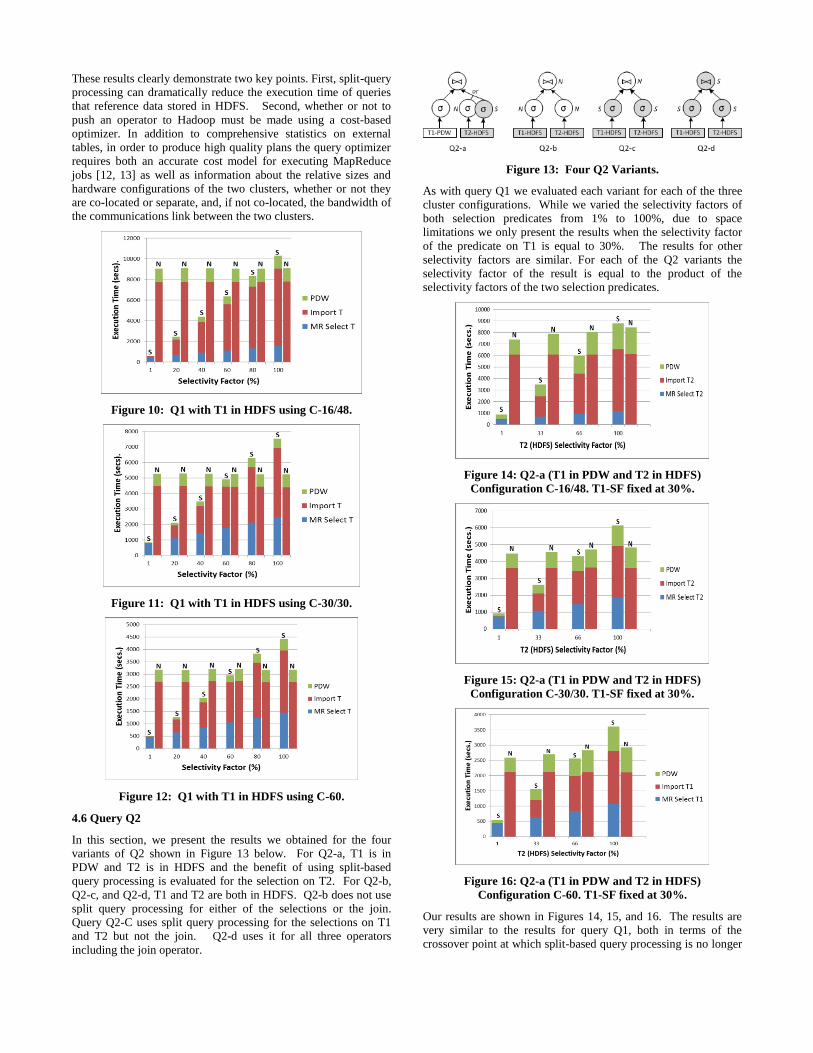
4.6 Query Q2

In this section, we present the results we obtained for the four

variants of Q2 shown in Figure 13 below. For Q2-a, T1 is in

PDW and T2 is in HDFS and the benefit of using split-based

query processing is evaluated for the selection on T2. For Q2-b,

Q2-c, and Q2-d, T1 and T2 are both in HDFS. Q2-b does not use

split query processing for either of the selections or the join.

Query Q2-C uses split query processing for the selections on T1

and T2 but not the join. Q2-d uses it for all three operators

including the join operator.

Figure 13: Four Q2 Variants.

As with query Q1 we evaluated each variant for each of the three

cluster configurations. While we varied the selectivity factors of

both selection predicates from 1% to 100%, due to space

limitations we only present the results when the selectivity factor

of the predicate on T1 is equal to 30%. The results for other

selectivity factors are similar. For each of the Q2 variants the

selectivity factor of the result is equal to the product of the

selectivity factors of the two selection predicates.

Figure 14: Q2-a (T1 in PDW and T2 in HDFS)

Configuration C-16/48. T1-SF fixed at 30%.

Figure 15: Q2-a (T1 in PDW and T2 in HDFS)

Configuration C-30/30. T1-SF fixed at 30%.

Figure 16: Q2-a (T1 in PDW and T2 in HDFS)

Configuration C-60. T1-SF fixed at 30%.

Our results are shown in Figures 14, 15, and 16. The results are

very similar to the results for query Q1, both in terms of the

crossover point at which split-based query processing is no longer

faster as well as the relative performance for the three

configurations.

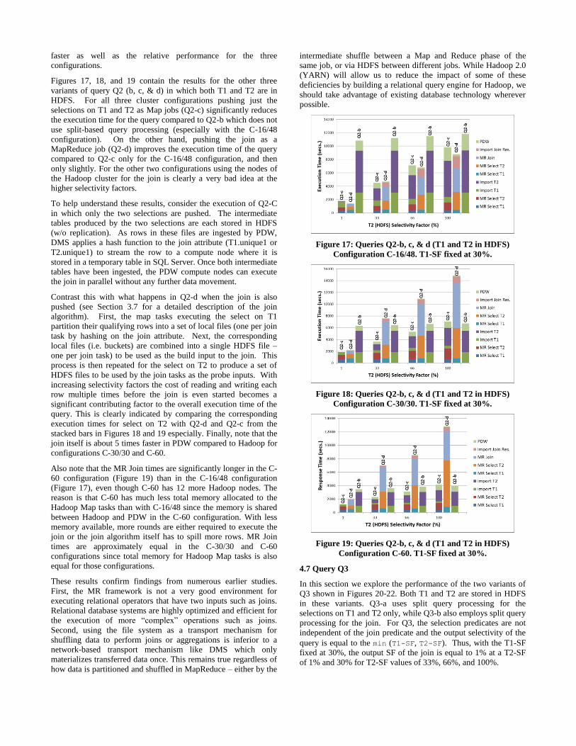
Figures 17, 18, and 19 contain the results for the other three

variants of query Q2 (b, c, & d) in which both T1 and T2 are in

HDFS. For all three cluster configurations pushing just the

selections on T1 and T2 as Map jobs (Q2-c) significantly reduces

the execution time for the query compared to Q2-b which does not

use split-based query processing (especially with the C-16/48

configuration). On the other hand, pushing the join as a

MapReduce job (Q2-d) improves the execution time of the query

compared to Q2-c only for the C-16/48 configuration, and then

only slightly. For the other two configurations using the nodes of

the Hadoop cluster for the join is clearly a very bad idea at the

higher selectivity factors.

To help understand these results, consider the execution of Q2-C

in which only the two selections are pushed. The intermediate

tables produced by the two selections are each stored in HDFS

(w/o replication). As rows in these files are ingested by PDW,

DMS applies a hash function to the join attribute (T1.unique1 or

T2.unique1) to stream the row to a compute node where it is

stored in a temporary table in SQL Server. Once both intermediate

tables have been ingested, the PDW compute nodes can execute

the join in parallel without any further data movement.

Contrast this with what happens in Q2-d when the join is also

pushed (see Section 3.7 for a detailed description of the join

algorithm). First, the map tasks executing the select on T1

partition their qualifying rows into a set of local files (one per join

task by hashing on the join attribute. Next, the corresponding

local files (i.e. buckets) are combined into a single HDFS file –

one per join task) to be used as the build input to the join. This

process is then repeated for the select on T2 to produce a set of

HDFS files to be used by the join tasks as the probe inputs. With

increasing selectivity factors the cost of reading and writing each

row multiple times before the join is even started becomes a

significant contributing factor to the overall execution time of the

query. This is clearly indicated by comparing the corresponding

execution times for select on T2 with Q2-d and Q2-c from the

stacked bars in Figures 18 and 19 especially. Finally, note that the

join itself is about 5 times faster in PDW compared to Hadoop for

configurations C-30/30 and C-60.

Also note that the MR Join times are significantly longer in the C-

60 configuration (Figure 19) than in the C-16/48 configuration

(Figure 17), even though C-60 has 12 more Hadoop nodes. The

reason is that C-60 has much less total memory allocated to the

Hadoop Map tasks than with C-16/48 since the memory is shared

between Hadoop and PDW in the C-60 configuration. With less

memory available, more rounds are either required to execute the

join or the join algorithm itself has to spill more rows. MR Join

times are approximately equal in the C-30/30 and C-60

configurations since total memory for Hadoop Map tasks is also

equal for those configurations.

These results confirm findings from numerous earlier studies.

First, the MR framework is not a very good environment for

executing relational operators that have two inputs such as joins.

Relational database systems are highly optimized and efficient for

the execution of more “complex” operations such as joins.

Second, using the file system as a transport mechanism for

shuffling data to perform joins or aggregations is inferior to a

network-based transport mechanism like DMS which only

materializes transferred data once. This remains true regardless of

how data is partitioned and shuffled in MapReduce – either by the

intermediate shuffle between a Map and Reduce phase of the

same job, or via HDFS between different jobs. While Hadoop 2.0

(YARN) will allow us to reduce the impact of some of these

deficiencies by building a relational query engine for Hadoop, we

should take advantage of existing database technology wherever

possible.

Figure 17: Queries Q2-b, c, & d (T1 and T2 in HDFS)

Configuration C-16/48. T1-SF fixed at 30%.

Figure 18: Queries Q2-b, c, & d (T1 and T2 in HDFS)

Configuration C-30/30. T1-SF fixed at 30%.

Figure 19: Queries Q2-b, c, & d (T1 and T2 in HDFS)

Configuration C-60. T1-SF fixed at 30%.

4.7 Query Q3

In this section we explore the performance of the two variants of

Q3 shown in Figures 20-22. Both T1 and T2 are stored in HDFS

in these variants. Q3-a uses split query processing for the

selections on T1 and T2 only, while Q3-b also employs split query

processing for the join. For Q3, the selection predicates are not

independent of the join predicate and the output selectivity of the

query is equal to the min (T1-SF, T2-SF). Thus, with the T1-SF

fixed at 30%, the output SF of the join is equal to 1% at a T2-SF

of 1% and 30% for T2-SF values of 33%, 66%, and 100%.

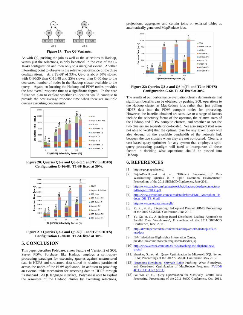
Figure 17: Two Q3 Variants.

As with Q2, pushing the join as well as the selections to Hadoop,

versus just the selections, is only beneficial in the case of the C-

16/48 configuration and then only to a marginal extent. Another

interesting point to observe is the relative performance of the three

configurations. At a T2-SF of 33%, Q3-b is about 50% slower

with C-30/30 than C-16/48 and 25% slower than C-60 due to the

decreased number of nodes in the Hadoop cluster available to the

query. Again, co-locating the Hadoop and PDW nodes provides

the best overall response time to a significant degree. In the near

future we plan to explore whether co-location would continue to

provide the best average response time when there are multiple

queries executing concurrently.

Figure 20: Queries Q3-a and Q3-b (T1 and T2 in HDFS)

Configuration C-16/48. T1-SF fixed at 30%.

Figure 21: Queries Q3-a and Q3-b (T1 and T2 in HDFS)

Configuration C-30/30. T1-SF fixed at 30%.

5. CONCLUSION

This paper describes Polybase, a new feature of Version 2 of SQL

Server PDW. Polybase, like Hadapt, employs a split-query

processing paradigm for executing queries against unstructured

data in HDFS and structured data stored in relations partitioned

across the nodes of the PDW appliance. In addition to providing

an external table mechanism for accessing data in HDFS through

its standard T-SQL language interface, Polybase is able to exploit

the resources of the Hadoop cluster by executing selections,

projections, aggregates and certain joins on external tables as

automatically generated MapReduce jobs.

Figure 22: Queries Q3-a and Q3-b (T1 and T2 in HDFS)

Configuration C-60. T1-SF fixed at 30%.

The results of our performance evaluation clearly demonstrate that

significant benefits can be obtained by pushing SQL operations to

the Hadoop cluster as MapReduce jobs rather than just pulling

HDFS data into the PDW compute nodes for processing.

However, the benefits obtained are sensitive to a range of factors

include the selectivity factor of the operator, the relative sizes of

the Hadoop and PDW compute clusters, and whether or not the

two clusters are separate or co-located. We also suspect (but were

not able to verify) that the optimal plan for any given query will

also depend on the available bandwidth of the network link

between the two clusters when they are not co-located. Clearly, a

cost-based query optimizer for any system that employs a split-

query processing paradigm will need to incorporate all these

factors in deciding what operations should be pushed into

Hadoop.

6. REFERENCES

[1] http://sqoop.apache.org

[2] Bajda-Pawlikowski, et. al., “Efficient Processing of Data Warehousing Queries in a Split Execution Environment,”

Proceedings of the 2011 SIGMOD Conference, June 2011.

[3] http://www.oracle.com/technetwork/bdc/hadoop-loader/connectors-

hdfs-wp-1674035.pdf

[4] http://www.greenplum.com/sites/default/files/EMC_Greenplum_Hadoop_DB_TB_0.pdf

[5] http://www.asterdata.com/sqlh/

[6] Yu Xu, et. al., Integrating Hadoop and Parallel DBMS, Proceedings of the 2010 SIGMOD Conference, June 2010.

[7] Yu Xu, et. al., A Hadoop Based Distributed Loading Approach to Parallel Data Warehouses", Proceedings of the 2011 SIGMOD

Conference, June, 2011.

[8] http://developer.teradata.com/extensibility/articles/hadoop-dfs-to-teradata

[9] IBM InfoSphere BigInsights Information Center,

pic.dhe.ibm.com/infocenter/bigins/v1r4/index.jsp

[10] http://www.vertica.com/2012/07/05/teaching-the-elephant-new-tricks/,

[11] Shankar, S., et. al., Query Optimization in Microsoft SQL Server

PDW, Proceedings of the 2012 SIGMOD Conference, May 2012.

[12] Herodotos Herodotou, Shivnath Babu: Profiling, What-if Analysis, and Cost-based Optimization of MapReduce Programs. PVLDB

4(11):1111-1122 (2011).

[13] Sai Wu, et. al., Query Optimization for Massively Parallel Data

Processing, Proceedings of the 2011 SoCC Conference, Oct. 2011.