SPSS TRAINING

SPSS “VIEWS”

Dataset – Data file ‐ Data View

o Full data set, structured same as excel (variable = column name, row = record) ‐ Variable View

o Provides details for each variable (column in Data view) – such as the variable type, and the type of measurement.

Output – Output of analysis file ‐ All steps you take recorded here

‐ Can make new outputs and save key steps in analysis this way 

Syntax – SPSS language,

‐ write and develop more tailored SPSS analysis without being restricted by “buttons” ‐ Useful when you know you want to repeat the same analysis later

o For example – first couple of weeks of data collection, all the variables are there – can set up the analysis syntax, prior to dataset completion and, providing variable names the same, can just simply “run” analysis as soon as have full cleaned dataset.

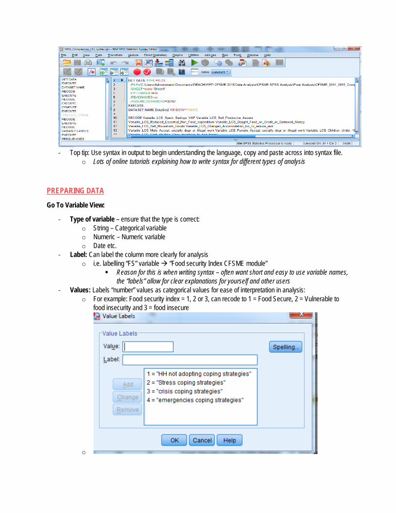
‐ Top tip: Use syntax in output to begin understanding the language, copy and paste across into syntax file.

o Lots of online tutorials explaining how to write syntax for different types of analysis

PREPARING DATA

Go To Variable View:

‐ Type of variable – ensure that the type is correct: o String – Categorical variable o Numeric – Numeric variable o Date etc.

‐ Label: Can label the column more clearly for analysis o i.e. labelling “FS” variable “Food security Index CFSME module”

Reason for this is when writing syntax – often want short and easy to use variable names, the “labels” allow for clear explanations for yourself and other users

‐ Values: Labels “number” values as categorical values for ease of interpretation in analysis: o For example: Food security index = 1, 2 or 3, can recode to 1 = Food Secure, 2 = Vulnerable to

food insecurity and 3 = food insecure

o

‐ Missing: depending on if string or numeric can tell SPSS what values should be counted as missing i.e. “NA” or “Null”.

‐ Measure: Useful for when conducting analysis and ensure different statistical tests can be used for variable o Nominal = categorical variables like governorate o Ordinal = ordered categorical variables like satisfaction

Go to “Data” in the top left bar for options:

Often, prior to the start of analysis, we want to ensure certain conditions are in place for the analysis, for example – weighting district samples according to their actual population size or using a filter to remove records which are not relevant for the decided course of analysis. The below outlines two key functions often used to set data prior to analysis.

WEIGHTING RECORDS – Often when conducting large nation-wide assessments, sample has been stratified for findings statistically significant at district level. Because samples are not proportion to actual population size, when then trying to conduct nation-wide analysis, districts with larger samples, in comparison to their actual population size, will be unfairly weighted in results. Therefore need to apply “district weights” to ensure that the nation-wide analysis is correctly reflected of the actual population, as distributed across the districts.

‐ Go to “data” in the top left bar for options ‐ Select in the dropdown list select “weight cases” ‐ In the box that appears, click on :”weight cases by” ‐ Select the variables in the left hand column which you’d like to weight each record by ‐ Click on the arrow in the right hand side of the box to select cases to be weighted by relevant variable ‐ Click OK

FILTERS – For some analysis we only wish to examine specific types of records. For example – in a nation-wide assessment, only examining records living in the “Host community” and excluding “camps” from the analysis.

‐ Go to “data” in the top left bar for options ‐ Select in the dropdown list select “select cases” ‐ In the box that appears, click on “If..” ‐ Type in the box what you want to include in analysis ‐ Click “OK” and only relevant records will be selected for analysis

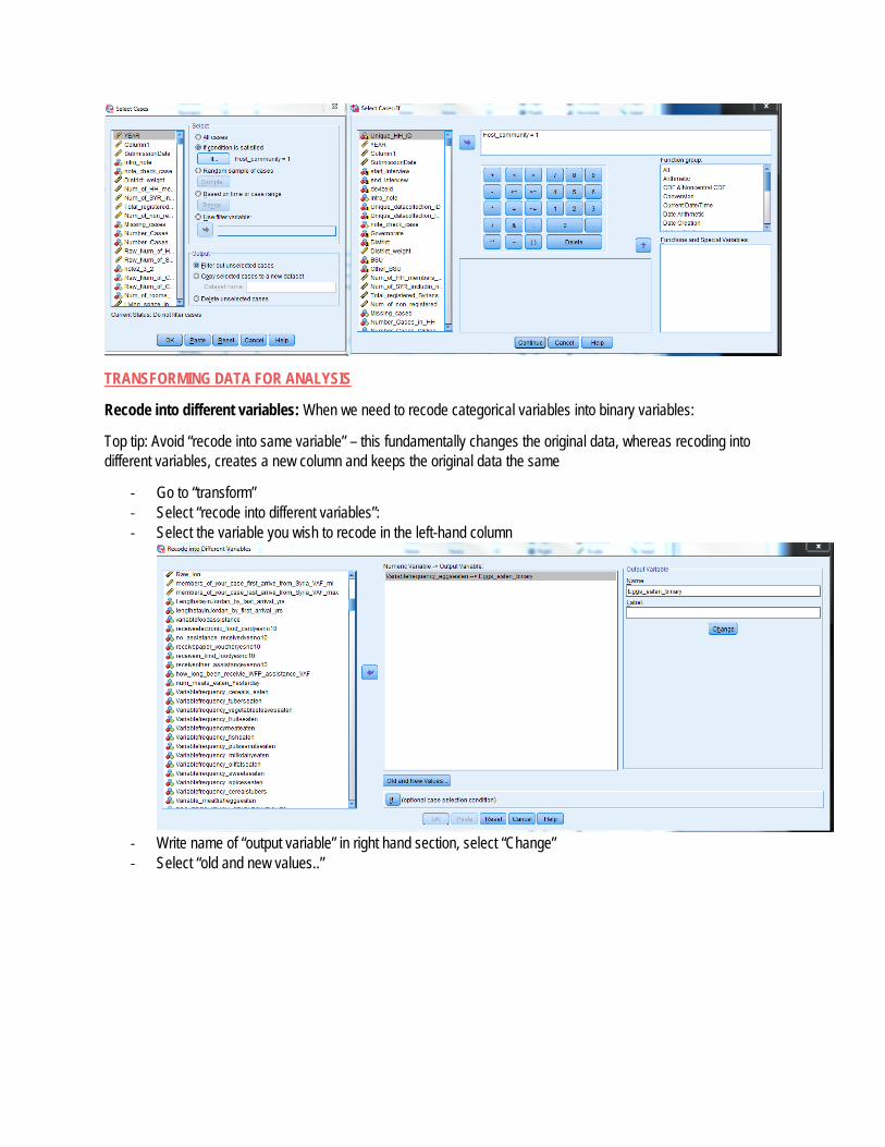
TRANSFORMING DATA FOR ANALYSIS

Recode into different variables: When we need to recode categorical variables into binary variables:

Top tip: Avoid “recode into same variable” – this fundamentally changes the original data, whereas recoding into different variables, creates a new column and keeps the original data the same

‐ Go to “transform” ‐ Select “recode into different variables”: ‐ Select the variable you wish to recode in the left-hand column

‐ Write name of “output variable” in right hand section, select “Change” ‐ Select “old and new values..”

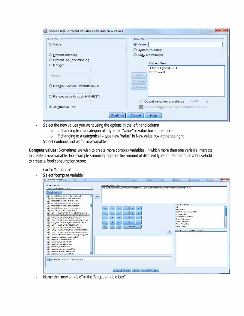
‐ Select the new values you want using the options in the left hand column

o If changing from a categorical – type old “value” in value box at the top left o If changing to a categorical – type new “value” in New value box at the top right

‐ Select continue and ok for new variable

Compute values: Sometimes we wish to create more complex variables, in which more than one variable interacts to create a new variable. For example summing together the amount of different types of food eaten in a household to create a food consumption score:

‐ Go To “transorm” ‐ Select “compute variable”

‐ Name the “new variable” in the “target variable box”

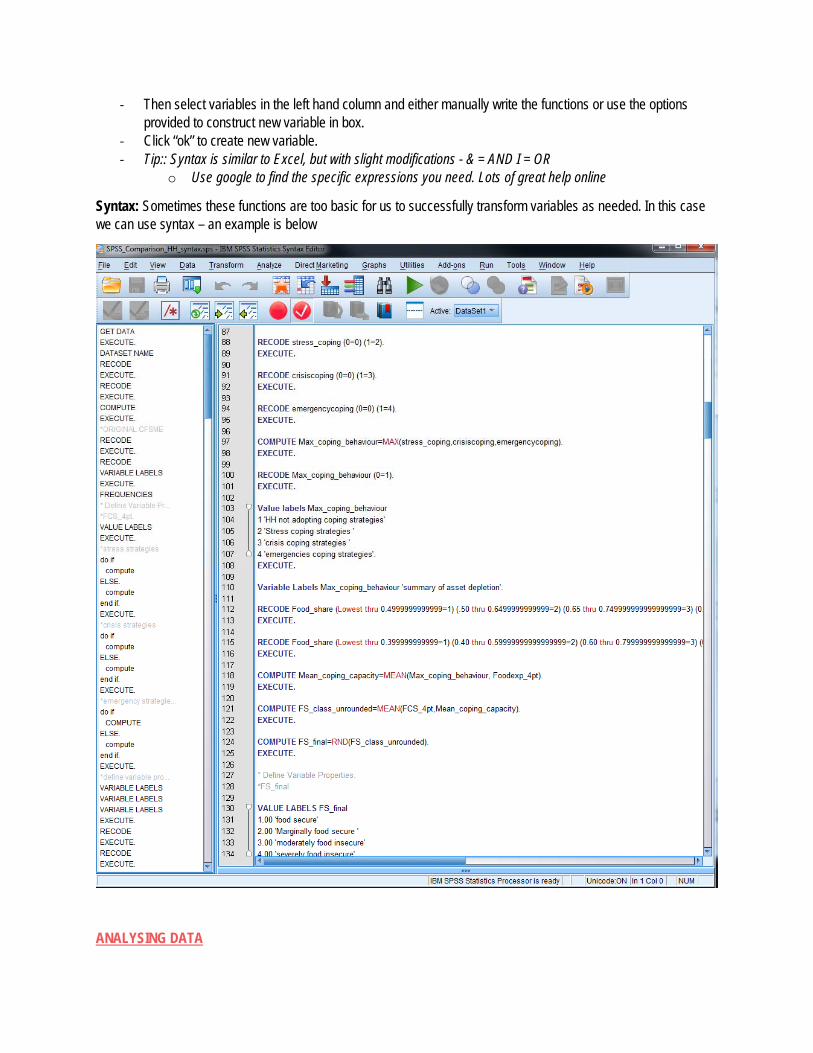
‐ Then select variables in the left hand column and either manually write the functions or use the options provided to construct new variable in box.

‐ Click “ok” to create new variable. ‐ Tip:: Syntax is similar to Excel, but with slight modifications - & = AND I = OR

o Use google to find the specific expressions you need. Lots of great help online

Syntax: Sometimes these functions are too basic for us to successfully transform variables as needed. In this case we can use syntax – an example is below

ANALYSING DATA

There are multiple functions on SPSS which can be used to analyse data, the majority of which fall under the “analyse” option in the top bar. Below go through the most basic and commonly used types of analysis.

BASIC DESCRIPTIVES FOR CATEGORICAL AND NUMERICAL VARIABLES:

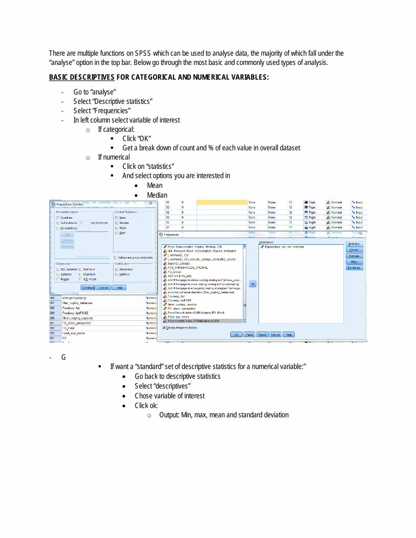
‐ Go to “analyse” ‐ Select “Descriptive statistics” ‐ Select “Frequencies” ‐ In left column select variable of interest

o If categorical: Click “OK” Get a break down of count and % of each value in overall dataset

o If numerical Click on “statistics” And select options you are interested in

Mean Median

‐ G

If want a “standard” set of descriptive statistics for a numerical variable:” Go back to descriptive statistics Select “descriptives” Chose variable of interest Click ok:

o Output: Min, max, mean and standard deviation

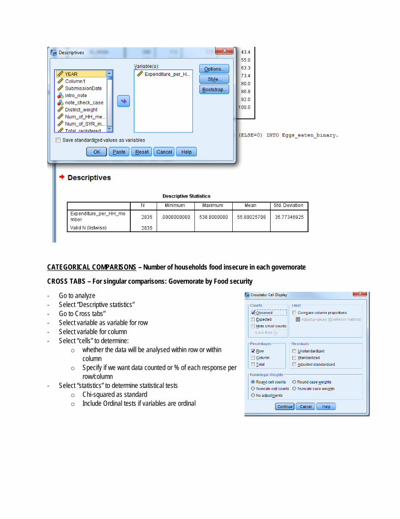
CATEGORICAL COMPARISONS – Number of households food insecure in each governorate

CROSS TABS – For singular comparisons: Governorate by Food security

‐ Go to analyze ‐ Select “Descriptive statistics” ‐ Go to Cross tabs” ‐ Select variable as variable for row ‐ Select variable for column ‐ Select “cells” to determine:

o whether the data will be analysed within row or within column

o Specify if we want data counted or % of each response per row/column

‐ Select “statistics” to determine statistical tests o Chi-squared as standard o Include Ordinal tests if variables are ordinal

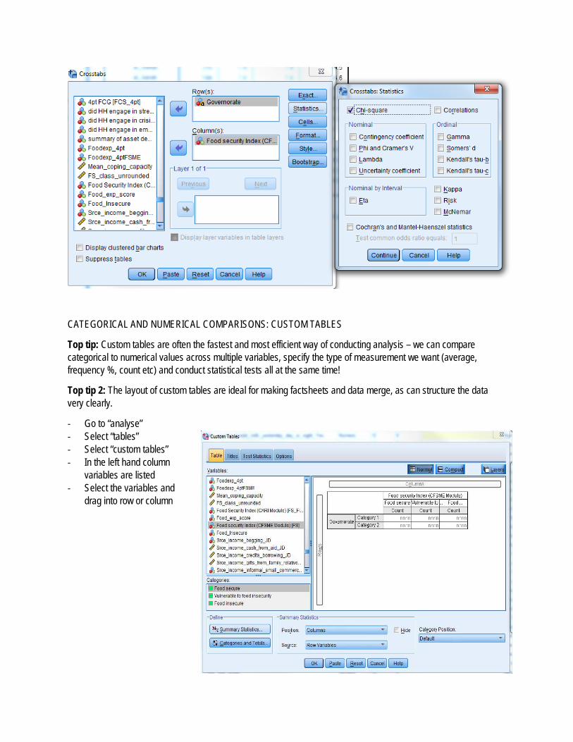
CATEGORICAL AND NUMERICAL COMPARISONS: CUSTOM TABLES

Top tip: Custom tables are often the fastest and most efficient way of conducting analysis – we can compare categorical to numerical values across multiple variables, specify the type of measurement we want (average, frequency %, count etc) and conduct statistical tests all at the same time!

Top tip 2: The layout of custom tables are ideal for making factsheets and data merge, as can structure the data very clearly.

‐ Go to “analyse” ‐ Select “tables” ‐ Select “custom tables” ‐ In the left hand column

variables are listed ‐ Select the variables and

drag into row or column

‐ Once we have a basic table ‐ Select “summary statistics” ‐ In the left hand column, select the type of analysis to be conducted (different options are available for either

categorical or numerical values)

‐ You can select more than one (frequency % and count might be useful) ‐ For numerical values you can select Average, sum, range, minimum and maximum etc.

Multiple custom table analysis

‐ We can analyse multiple different variables by the governorate variable ‐ Simply drag new variables into the column and it will be added to the table (and analyzed separately) ‐ Keep checking the “summary statistics” options to change the type of analysis produced

Top tip: Custom tables can also be used to aggregate large datasets or merge looped sheets from ODK forms. For example if “metainstance ID” is the unique HH record, and is included in the sheet for HH member details. Select “metainstance ID” as row record variable and then we can sum the number of HH members working in the column.