stability and system time distribution of dynamiccpcc.berkeley.edu/papers/dtrp.pdf · stability and...

STABILITY AND SYSTEM TIME DISTRIBUTION OF DYNAMICTRAVELING REPAIRMAN PROBLEM∗

JIANGCHUAN HUANG† AND RAJA SENGUPTA‡

Abstract. A good model for the dynamic vehicle routing problem is the Dynamic TravelingRepairman Problem (DTRP) [4]. The DTRP literature has focused on optimizing the expected valueof system time, defined as the elapsed time between the arrival and the completion of each task. Wefocus on the stability and distribution of system time, including its variance. This paper establishes apartially policy independent necessary and sufficient condition for stability in the DTRP. The policyclass includes some of the policies proven to be optimal for system time expectation under light andheavy loads in the literature. We propose a new policy named PART-n-TSP and compute a goodapproximation for its system time distribution. PART-n-TSP has lower system time variance thanPART-TSP [31] and Nearest Neighbor [4] when the load is neither too small or too large. We provethat PART-n-TSP is also optimal for system time expectation under light and heavy loads.

Key words. Dynamic Traveling Repairman Problem, Polling Systems, Economy of Scale

1. Introduction. Dynamic vehicle routing problems arise when one needs toserve tasks that arrive in time and space. The objective is to schedule the tasks inan economic way to achieve good service level according to some performance metric,e.g., average waiting time, throughput, delivery probability of the tasks, or the totaldistance traveled by the moving servers (vehicles). There are many practical appli-cation where the dynamic vehicle routing problems arise. For example, (i) GoogleStreet View, Google is running numerous data-collection vehicles with mounted cam-eras, lasers, a GPS and several computers to collect street views while minimizing thedistance travelled [2]. (ii) Real-time traffic reporting, a radio station uses a helicopterto overfly accident scenes and other areas of high traffic volume for real-time traf-fic information. (iii) Unmanned aerial vehicle (UAV)-based sensing, a fleet of UAVsequipped with greenhouse gas sensors collect airborne measurements of greenhousegases at several sites in California and Nevada, executing every task at its locationbefore its deadline [18]. (iv) Enabling mobility in wireless sensor networks (WSN),mobile elements (vehicles) capable of short-range communications collect data fromnearby sensor nodes as they approach on a schedule [23].

The Dynamic Traveling Repairman Problem (DTRP) [4] is a good way to modelthe dynamic vehicle routing problem: A convex region A of area A contains a vehicle(server) that travels at constant speed v. Tasks arrive according to a Poisson processwith rate λ. Each task i is located at Xi ∈ A, and has size Bi. Xi is independent andidentically distributed (i.i.d.) with probability density function (pdf) fX(x), x ∈ A.Bi is i.i.d. with pdf fB(s), s ∈ [0,∞). E [Bi] = b, which is assumed to be finite.Define load ρ = λb . The system time of task i, denoted Ti, is defined as the elapsedtime between the arrival of task i and the time task i is completed. It is a measureof system performance. An earlier formulation similar to the DTRP can be found in[10].

The DTRP resembles an M/G/1 queue in the time dimension but looks like avehicle routing problem in the space dimension. As we know in queueing theory,

∗This work was partly supported by NSF-CNS-1136141.†Systems Engineering Group, Department of Civil and Environmental Engineering, University of

California at Berkeley ([email protected]).‡Systems Engineering Group, Department of Civil and Environmental Engineering, University of

California at Berkeley.

1

2 JIANGCHUAN HUANG AND RAJA SENGUPTA

ρ = λb < 1 is a necessary and sufficient condition for all work conserving M/G/1queues [9, sec. II.4.2]. However, there is no such policy-independent stability conditionfor the DTRP, which seems to be a “spatial version” of the M/G/1 queue. The knownstability conditions for the DTRP are policy-dependent [4, 31, 20].

This paper makes progress towards finding stability conditions for the DTRP thatare less policy dependent than those in the literature. We establish ρ + λbd < 1 asa necessary and sufficient stability condition for the class of Polling-Sequencing (P-S) policies satisfying unlimited-polling and economy of scale in Theorem 2.12. Thisstability condition is identical to the necessary condition for stability given in [5]. Weshow that important policies for the DTRP in the literature fall in the P-S class andsatisfy the two properties. The extra term bd is the limit of mean travel time as thenumber of tasks in a polling station goes to infinity. We prove that the existence ofbd is a consequence of economy of scale. bd is policy-dependent, but it only dependson the sequencing phase of the P-S policy. Since the value of bd can be derived in thestatic setting, we do not need to analyze or simulate the dynamic queueing systemof DTRP to get bd. We only need to analyze or simulate to obtain the statisticsof sequencing N tasks, where N is a random variable, and the task locations aredistributed in some fashion.

Our second contribution to the DTRP is the distribution of system time T , definedas the elapsed time between the arrival and the completion of each task. Knowing thedistribution of the system time T , together with its expectation E[T ] and varianceV ar[T ] or standard deviation σ[T ], enables the expectation-variance analysis of thesystem under uncertainties [12, 22]. On entering a McDonalds, one may ask not just“What is my expected service time?” but also “How certain is this value?” Weshow in Tables 3.1 and 3.2 in Section 3 that two policies at the same load level canbe incomparable in the sense that one has low expectation of system time but highvariance while the other has high expectation of system time but low variance. Inpractice, highly variable system time can be even more frustrating than large meansystem times [13, 17]. The literature discusses the distribution of system time T ,together with its expectation and variance, for the FCFS policy and its variationssuch as the SQM and partitioning-FCFS [4]. This is in sharp contrast to queueingtheory where the distribution of the system time or its moments are known for a widevariety of policies. See for example [26, 30]. To illustrate our point, the expectedsystem time of the FCFS, SQM and partitioning-FCFS policy is not as good as NN[4] and PART-TSP [31] or DC [20] at most load levels.

In Section 3, we propose a policy in the P-S class called the PART-n-TSP policy.We give a good approximation for the distribution of the system time that is easyto compute. We do this by utilizing approximation results for the distribution ofsystem time T , together with E[T ] and V ar[T ] known for polling systems [8, 15].Figure 3.5 shows that the cumulative distribution function (cdf) of the system timeas computed by our method is very close to the cdf of the system time as obtained byMonte-Carlo simulation. We show that FCFS, partitioning-FCFS and n-TSP [4] arespecial cases of PART-n-TSP, meaning PART-n-TSP can be optimized to have betterperformance than the three. We also compare PART-n-TSP with PART-TSP [31]and Nearest Neighbor [4] on E[T ] and σ[T ] in Tables 3.1 and 3.2, since the latter twoare considered near optimal in the literature. The E[T ] and σ[T ] under PART-n-TSPare obtained by our approximation. The E[T ] and σ[T ] under PART-TSP and NNare obtained by simulation. The results show that NN achieves lower E[T ] than bothPART-n-TSP and PART-TSP for all loads ρ ∈ 0.1 . . . 0.9 simulated by us. PART-

STABILITY AND SYSTEM TIME DISTRIBUTION OF DTRP 3

n-TSP achieves lower E[T ] than PART-TSP when ρ is not too small or too large, e.g.when ρ ∈ 0.3, . . . , 0.7. Also, PART-n-TSP achieves lower σ[T ] than PART-TSP andNN when ρ is not too small or too large, e.g. when ρ ∈ 0.3, . . . , 0.7. In real systemsit may be desirable for ρ to be neither too small nor too large, since small ρ results inlow server utilization, and large ρ in large system times. If so, PART-n-TSP would begood in practice as it achieves lower σ[T ] than PART-TSP and NN, and lower E[T ]than PART-TSP. We also prove that PART-n-TSP is E[T ] optimal under light load(ρ→ 0+) and asymptotically optimal under heavy load (ρ→ 1−). See Theorem 3.2.

2. Polling-Sequencing Policies. The class of Polling-Sequencing (P-S) poli-cies include a polling phase and a sequencing phase. For the notation of P-S policies,we use “PART-” to denote the polling (partitioning) phase, followed with the sequenc-ing policies for the sequencing phase. For example, PART-TSP means first partitionthe region A into polling stations, and use TSP to sequence the tasks inside eachpolling station. Similarly, we can define PART-NN, PART-SJF, etc.

2.1. Spatial-Polling: Markov Chain. Polling policies are well-established inthe queueing theory literature. Overviews and surveys of polling systems can be foundin [25, 27, 29]. Stability and ergodicity criteria for polling systems are well establishedand can be found in [1, 16, 21, 7].

The polling phase of the P-S class is a spatial-polling policy, we divide the region Ainto an r-partition Akrk=1, each of area Ak. We label the r partitions as 1, 2, . . . , r.We regard each partition as a station in classic polling systems. In this way wegeneralize the polling system [1, 16] in classic queueing theory to the spatial case.

The vehicle visits the partitions in cyclic order, 1, 2, . . . , r, 1, 2, . . ., and serves thetasks in each partition. Without loss of generality, we assume that the vehicle isinitially at partition 1. Thus, the l-th visit of the vehicle is partition I(l) = (l − 1)(mod r) + 1, where l (mod r) means the remainder of the division of l by r. The setof tasks waiting in partition I(l) on the arrival of the l-th visit of the vehicle is calledthe l-th queue (the queue observed at l-th visit).

We denote by:Gk(N) the number of tasks that are served in partition k when the queue observed

is of length N .T kS (n) the total service time of n tasks in partition k. The formal definition of

function T kS (.) will be given in section 2.2.Sk(N) the duration of the service in partition k when the queue observed is of

length N .

Sk(N) = T kS(Gk(N)

)(2.1)

Function Gk(.) characterizes the polling policy and T kS (.) characterizes the se-quencing policy.

The switch time the vehicle takes from a random point in partition k to a randompoint in partition k+ 1 is denoted by ∆k, k = 1, . . . , r− 1. The value from partition rto partition 1 is denoted by ∆r. ∆k, k = 1, . . . , r, are bounded above by the diameterof the region A divided by the speed of the vehicle v. The first moment of ∆k isdenoted by δk, k = 1, . . . , r. Let ∆ =

∑rk=1 ∆k be the total switch time in a cycle

and denote by δ the first moment of ∆.The tasks arrive at partition k with a Poisson process of parameter λk =

∫AkfX(x) dxλ.

The task sizes are i.i.d. with common distribution B and mean b. Define ρk = λkb,and ρ =

∑rk=1 ρ

k, 1 ≤ k ≤ r. Let Nk (t1, t2] denote the number of Poisson arrivals to


partition k, 1 ≤ k ≤ r, during a (random) time interval (t1, t2]. Nk(t) ≡ Nk (0, t] isthe number of Poisson arrivals in a time interval of length t.

The l-th value of the polling system is described by the random variables Nkl ,

1 ≤ k ≤ r, l ≥ 1, where Nkl represents the number of tasks in partition k at the l-th

visit of the vehicle. Let Nl =(N1l , . . . , N

rl

), taking values in Nr, where N is the set

of nonnegative integers.Denote by Sl, the station time, the time interval between the arrival times of the

l-th visit and the (l + 1)st visit of the vehicle.

Sl = SI(l)(NI(l)l ) + ∆I(l)(2.2)

Denote by Cl, the cycle time, the time interval between two successive arrivals ofthe vehicle to the same partition. Cl = Sl + . . .+ Sl+r−1.

The arrival times, the service times, the switch times are mutually independent,and are independent of the past and present system states. We adopt the rigorousindependence definitions from Fricker [16] with some changes for the spatial case.

Consider a queue service starting at stopping time τ at partition k while N tasksare waiting and N− tasks have already been served for the whole system. Let Fτbe any σ-field containing the history of the service process up to random time τ .Fτ is independent of the process N(τ, τ + .] of arrivals after τ and of the task sizesBN−+ii>0 of the tasks that have not been served up to time τ . The following fourassumptions hold for all k = 1, . . . , r.

A1: (Gk, Sk) is conditionally independent of Fτ given N , and has the distributionof(Gk(N), Sk(N)

)where the expressions of the random functions (Gk(.), T kS (.)) are

taken independent of N . i.e. The A-S policies do not depend on the past history ofthe service process such as the number of tasks being already served and the timespent serving them.

A2: (Gk, Sk) is independent of((BN−+Gk+i)i>0 , N

(τ + Sk, τ + Sk + .

]), i.e. The selection of a task for service is

independent of the required execution time and of possible future arrivals.A3: Gk(0) = 0, Sk(0) = 0 and there exists N > 0 such that Gk(N) > 0. i.e. The

vehicle leaves immediately a queue which is or becomes empty, but provides servicewith a positive probability once there are “enough” task(s) in the queue.

A4:(Gk(N), Sk(N)

)is monotonic and contractive in N . A function g(.) is

contractive if for every x ≥ y, g(x)− g(y) ≤ x− y.Nl evolve according to the following evolution equations:

Nkl+1 =

Nkl +Nk (Sl) , if I(l) 6= k

Nkl −Gk

(Nkl

)+Nk (Sl) , if I(l) = k

(2.3)

where I(l) = (l − 1) (mod r) + 1.The spatial polling system has a Markovian structure as specified by the following

two theorems, which is almost identical to the theorems given in [16].Theorem 2.1. The sequence Nl∞l=0 is a Markov chain.Proof. At the l-th polling instant τ , the server starts serving queue l (if not

empty, otherwise he starts switching to queue l + 1) according to policy GI(l) whilethe state of all queues is given by Nl. The arrival processes after l are Poisson andare independent of Fτ ; the service times and the switch times involved after τ arealso independent of Fτ . Because these quantities are mutually independent, it followsthat given Nl, the evolution of the system after τ is independent of Fτ , which ensuresthe Markov property of the sequence.


Remark 2.1.1. This Markov chain is in general not homogeneous because itstransitions depend on l through GI(l) and ∆I(l), and I(l) is different for each l. Onecan check that theorem 2.1 also holds when the task arrival process is renewal. Thisguarantees the arrival processes after l are independent of Fτ .

Theorem 2.2. Nlr+k∞l=0 is a homogeneous, irreducible and aperiodic Markovchain with state space Nr, k = 1, . . . , r, where r is the number of polling stations.

Proof. Nlr+k∞l=0 is a subsequence of the Markov chain Nl∞l=0 and is thus alsoa Markov chain which is homogeneous because I(lr + k) = k and GI(lr+k) = Gk forl = 0, 1, 2, . . ..

It is irreducible because all states communicate. Indeed,(N1, . . . , Nr

)can be

reached in one step from the state (0, . . . , 0): this is realized when first no arrivalsoccur to all queues during the whole cycle but the last switch time ∆r−1, and thenthe last switch time is positive and

(N1, . . . , Nr

)arrivals occur during it, all this

having a positive probability because the arrival processes are Poisson. On the otherhand, (0, . . . , 0) is reached in (possibly) many steps from any state

(N1, . . . , Nr

)with

positive probability too: this is realized when there are no arrivals until it happens.By the same arguments, the state (0, . . . , 0) is aperiodic and so is the (irreducible)Markov chain.

2.2. Sequencing: Economy of Scale. Under a spatial-polling policy, the num-ber and locations of tasks are determined in each polling station in each polling cycle,which is a static vehicle routing problem. The sequencing policies sequence the set oftasks in each polling station.

Definition 2.3. A policy for the 1-DTRP is called a Polling-Sequencing (P-S)policy if it runs a spatial-polling policy in region A, and sequences the set of tasks ineach polling station using some sequencing policy.

For a set of n tasks Bi, Xini=1, each with size Bi and location Xi, denote byTPD (Xini=1) and TPS (Bi, Xini=1) the travel time and service time for the n tasksBi, Xini=1 under sequencing policy P .

TPD (Xini=1) ≡ EX[

1

vDP (X, Xini=1)

](2.4)

where v is the vehicle speed, and DP (X, Xini=1) is the distance travelled by thevehicle to serve the tasks Bi, Xini=1 starting from a random point X in region Aunder sequencing policy P .

TPS (Bi, Xini=1) = TPD (Xini=1) +

n∑i=1

Bi(2.5)

Define TPD (n) ≡ EXi[TPD (Xini=1)

],

and TPS (n) ≡ EXi[EBi

[TPS (Bi, Xini=1)

]], then

TPS (n) = TPD (n) + nb(2.6)

T kS (n) ≡ TPS (n) and T kD(n) ≡ TPD (n) when sequencing policy P is used in partition k.Definition 2.4. A sequencing policy P is said to have economy of scale (EoS)

ifTPD (n)n is nonincreasing in n.Definition 2.5. A scheduling policy is called non-location based if the distance

between two consecutively executed tasks is i.i.d.. A scheduling policy is called locationbased if the distance between two consecutively executed tasks is dependent.


Non-location based policies include FCFS, SJF, ROS and longest job first (LJF).Theorem 2.6(i) shows that non-location based policies satisfy economy of scale.

Location based policies include NN, furthest job first (FJF), TSP and the ap-proximation algorithms for TSP such as Daganzo’s algorithm (DA) [11]. For locationbased policies, there are two categories. One category try to find a shorter path con-necting the locations of the tasks, which we call smart. Examples include TSP, NNand the approximation algorithms of TSP such as Daganzo’s algorithm (DA) [11].The other category tries to find a longer path connecting the locations of the tasks,which we call foolish. Examples include furthest job first (FJF). This category doesnot has EoS, and is not practical. Theorem 2.6(ii) below proves that the commonpolicies in the smart category such as TSP, NN and DA have EoS. Other policies inthis category can be checked by the similar analysis or through simulation. Theorem2.6(ii) also proves that FJF does not satisfy EoS. NN and TSP are well known. InDA, one cuts a swath of approximate width, w, covering the region A. One possible

pattern is shown in the left of Figure 2.1 with a swath of width√A

6 . The vehicle visitsthe task locations by moving along the swath without backtracking.

Figure 2.1. Daganzo’s Algorithm, cited from [11].

Theorem 2.6. (i) Non-location based policies satisfy economy of scale. (ii)Nearest neighbor, traveling salesman policy and Daganzo’s algorithm in the locationbased policy class satisfy economy of scale, furthest job first in the location based policyclass does not satisfy economy of scale.

Proof. (i) This is because that Xi is independent of the arrival process, and Xi

is independent of Xi−1. Non-location based policies do not sequence based on the

locations of tasks, so TPD (n) = E[∑n

i=1Div

]=∑ni=1 E[Di]

v , where Di =‖ Xi −Xi−1 ‖when i > 1, D1 =‖ X1−Xv ‖, where Xi is the location of the i-th task and Xv is theinitial position of the vehicle. Xi and Xv are i.i.d. with pdf fX(x). Thus E [Di] is a

constant, say d. ThenTPD (n)n = nd

n = d, which is nonincreasing in n. So non-locationbased policies satisfy EoS.

(ii) Under TSP, when there are n tasks, there are n! Hamiltonian paths startingfrom the initial position of the vehicle. A Hamiltonian path is a path that visits eachXi exactly once. The length of each Hamiltonian path is the sum of n i.i.d. Di’s,HP =

∑ni=1Di. The TSP tour is the Hamiltonian path with minimum lengths among

the n! Hamiltonian paths. Let Ln be the tour length, thenTPD (n)n = E[Ln]

nv . Whenthere are n+ 1 tasks, there are (n+ 1)! Hamiltonian paths, and Ln+1 is the shortest

of them. P(Ln+1

n+1 > y)≤ P

(Lnn > y

)because Ln+1 is the minimum of (n + 1)!


Hamiltonian paths and Ln is the minimum of n! Hamiltonian paths. E[Ln+1]n+1 =∫∞

0P(Ln+1

n+1 > y)dy ≤

∫∞0P(Lnn > y

)dy = E[Ln]

n . ThenTPD (n+1)n+1 ≤ TPD (n)

n . TSP

satisfies EoS.Under NN, when there are n tasks, Let LNNn be the length of the tour connecting

the initial vehicle position and the locations of the n tasks, thenTPD (n)n =

E[LNNn ]nv .

LNNn is composed of n segments, LNNn =∑ni=1D

NNi , label i backwards such that

DNNi is the distance from the (n − i)-th point to the (n − i + 1)-th point when

i = 1, . . . , n− 1, and Dn is the distance from the initial position of the vehicle to the1st point. So DNN

i is the minimum of i Dj ’s, where each Dj is the distance betweentwo random points in the region A. Thus P

(DNNi+1 > y

)≤ P

(DNNi > y

), this implies

E[DNNi+1

]≤ E

[DNNi

], thus

E[LNNn+1]n+1 =

∑n+1i=1 E[DNNi ]

n+1 ≤∑ni=1 E[DNNi ]+

∑ni=1

1nE[DNNi ]

n+1 =∑ni=1

n+1n E[DNNi ]n+1 =

E[LNNn ]n . So

TPD (n+1)n+1 ≤ TPD (n)

n . NN satisfies EoS.In [11], the swath was approximated to be a infinitely long strip of width w

neglecting corner effect as shown in the right two of Figure 2.1. The mean travel time

per task when serving n tasks,TPD (n)n = ndw

n = dw, where dw is the expected distancebetween two consecutive locations. Let X denote the random distance between twoconsecutive points along the width of the strip, and Y the distance along the side of thestrip, then E[X] = w

3 , E[Y ] = Anw according to [11]. dw = EX,Y

(√X2 + Y 2

)for the

Euclidean metric. dw ≈ w3 + A

nwψ(nw2

A

), where ψ(x) = 2

x2 ((1 + x)log(1 + x)− x).

w∗ =√

2.95An minimizes dw. Substituting w∗, we see dw is decreasing with n. Thus

TPD (n)n is nonincreasing in n.

0 50 100 150 200 250 300 350 4000

0.1

0.2

0.3

0.4

0.5

Number of points n

Mea

n tra

vel t

ime,

TDP (n

)/n

Mean travel time under TSP, NN and DA

TSPNNDA

Figure 2.2. Mean travel time under TSP, NN and DA.

We show that FJF does not satisfy EoS by a counterexample. Consider a square

of size 1× 1 with uniformly distributed task locations.TPD (1)

1 = E[D1] = 0.52, whereD1 =‖ X1 − Xv ‖, where Xi is the location of the i-th task and Xv is the initialposition of the vehicle. Xi and Xv are i.i.d. with pdf fX(x) = 1. When there are two


tasks, the vehicle will choose the task further away, thusTPD (2)

2 > 0.52 =TPD (1)

1 . ThusFJF does not satisfy EoS.

Remark 2.6.1. Non-location based policies have trivial EoS in the sense thatTPD (n)n is a constant.

Theorem 2.6(ii) is supported by the simulation results in Figure 2.2. The simu-lations are done in a square A of size 1× 1. The task locations and the initial vehicleposition are generated independently from a uniform distribution with pdf fX(x) = 1.The length of the path connecting the vehicle and the tasks is calculated under TSP,NN and DA for different number of points n.

Theorem 2.7. Under a sequencing policy P with economy of scale, limn→∞TPD (n)n =

bd ≥ 0, and ∃M > 0, s.t. M ≥ TPD (n)n ≥ bd for all n.

Proof.TPD (n)n ≥ 0 and

TPD (n)n is nonincreasing in n imply that limn→∞

TPD (n)n exists,

say bd.

Thus we have limn→∞TPD (n)n = bd and M =

TPD (1)1 ≥ TPD (n)

n ≥ bd ≥ 0.

Remark 2.7.1. bd is a measure of how well the sequencing policy can take advan-tage of the task locations. Let Ln denote the length of the tour connecting n points in asquare of area A under TSP. From [24] we know that limn→∞

Ln√n

= βTSP√A, where

βTSP ≈ 0.72, thus bd = limn→∞TPD (n)n = limn→∞

E[Ln]vn = limn→∞ βTSP

√A

v√n

= 0.

This implies that TSP does best in taking advantage of the task locations.

2.3. Stability Condition. Stability of DTRP is more complicated than inqueueing theory because the stability of DTRP is policy dependent, whereas in queue-ing theory we have the policy-independent stability condition ρ < 1 for work conserv-ing M/G/1 queues. Theorem 2.1 and 2.2 showed that Nl∞l=0 is a Markov chain, andNlr+k∞l=0 is a homogeneous, irreducible and aperiodic Markov chain. We check theergodicity of Nlr+k∞l=0 and the stability of the DTRP under the P-S policies in thissection.

Definition 2.8. A polling policy characterized by Gk(.) is called an unlimited-polling policy if Gk(N)→∞, when N →∞, k = 1, . . . , r.

One can check that the common polling policies such as the exhaustive and gatedpolicies in [25] are unlimited-polling policies.

Lemma 2.9. (LEMMA 3.1 in [1]) If for all 1 ≤ k ≤ r the Markov chainsNlr+k∞l=0 are ergodic, then for all 1 ≤ k ≤ r Nlr+k∞l=0 together with the sequenceof station times Slr+k∞l=0 and the cycle times Clr+k∞l=0 converge weakly to finiterandom variables.

Definition 2.10. The DTRP under a P-S policy is said to be stable if all the rMarkov chains Nlr+k∞l=0 are ergodic.

Lemma 2.11. (Foster’s Criterion [3, p.19]): Suppose a Markov chain is irre-ducible and let E0 be a finite subset of the state space E. Then the chain is positiverecurrent if for some h : E → R and some ε > 0 we have infx h(x) > −∞ and

i)∑k∈E pjkh(k) <∞, j ∈ E0,

ii)∑k∈E pjkh(k) ≤ h(j)− ε, j /∈ E0.

where pjk is the transition probability of the chain.

Theorem 2.12. (Stability theorem): For any P-S policy with polling policy satis-

fying Definition 2.8 (unlimited-polling) and sequencing policy P satisfying limn→∞TkD(n)n =

bkd in each partition Ak, assuming the partitions Akrk=1 are divided such that

bkd = limn→∞TPD (n)n = bd, ∀1 ≤ k ≤ r, then when ρ+ λbd < 1, the Markov chains


Nlr+k∞l=0 are ergodic, ∀1 ≤ k ≤ r. Moreover, if the sequencing policy P satisfiesDefinition 2.4 (EoS), then ρ+ λbd < 1 is necessary for the ergodicity of Nlr+k∞l=0.

Proof. Sufficiency: taking a conditional expectation in (2.3), summing over k,and substituting (2.2) and (2.1) we obtain:

E[∑r

k=1 bNkl+1 |Nl

]=∑rk=1 bN

kl − bGI(l)

(NI(l)l

)+ E

[∑rk=1 bN

k(∆I(l)

)|Nl]

+ E[∑r

k=1 bNk(TI(l)S

(GI(l)

(NI(l)l

)))|Nl]

=∑rk=1 bN

kl − bGI(l)

(NI(l)l

)+ E

[∑rk=1 bN

k(∆I(l)

)]+∑rk=1 bE[Nk(

∑GI(l)(NI(l)l )

i=1 Bi + TI(l)D (GI(l)(N

I(l)l ))) |Nl ]

=∑rk=1 bN

kl − bGI(l)

(NI(l)l

)+∑rk=1 bλkE

[∆I(l)

]+∑rk=1 bλk

(GI(l)

(NI(l)l

)b+ T

I(l)D

(GI(l)

(NI(l)l

)))=∑rk=1 bN

kl − bGI(l)

(NI(l)l

)+∑rk=1 bλkδ

I(l)

+ ρ(GI(l)

(NI(l)l

)b+ TPD

(GI(l)

(NI(l)l

)))=∑rk=1 bN

kl + ρδI(l) +

(ρ− 1 + λ

TPD

(GI(l)

(NI(l)l

))GI(l)

(NI(l)l

) )bGI(l)

(NI(l)l

).

Define γk = ρ− 1 + λTPD

(GI(l+k)

(NI(l+k)l+k

))GI(l+k)

(NI(l+k)l+k

) , k = 0, . . . , r − 1,

then E[∑r

k=1 bNkl+1 |Nl

]=∑rk=1 bN

kl + ρδI(l) + γ0bGI(l)

(NI(l)l

).

Similarly, E[∑r

k=1 bNkl+2 |Nl

]= E

[E[∑r

k=1 bNkl+2 |Nl+1, Nl

]|Nl]

= E[E[∑r

k=1 bNkl+2 |Nl+1

]|Nl]

= E[∑r

k=1 bNkl+1 |Nl

]+ ρδI(l+1) + E

[γ1bGI(l+1)

(NI(l+1)l+1

)|Nl].

Since NI(l+1)l+1 = N

I(l+1)l +N I(l+1) (Sl) ≥ N I(l+1)

l ,and Gk(.) is nondecreasing, then

E[GI(l+1)

(NI(l+1)l+1

)|Nl]≥ E

[GI(l+1)

(NI(l+1)l

)|Nl]

= GI(l+1)(NI(l+1)l

).

ρ+ λbd < 1 implies ε1 = 1−ρ−λbdλ > 0.

Since limn→∞TPD (n)n = bd ≥ 0,

then ∃M1 > 0, s.t. n > M1 impliesTPD (n)n − bd < ε1, i.e. ρ− 1 + λ

TPD (n)n < 0.

Thus when GI(l+1)(NI(l+1)l

)> M1, GI(l+1)

(NI(l+1)l+1

)> M1, γ1 < 0.

This implies E[γ1bGI(l+1)

(NI(l+1)l+1

)|Nl]≤ γ1bGI(l+1)

(NI(l+1)l

).

So when GI(l+1)(NI(l+1)l

)> M1,

E[∑r

k=1 bNkl+2 |Nl

]≤ E

[∑rk=1 bN

kl+1 |Nl

]+ ρδI(l+1) + γ1bGI(l+1)

(NI(l+1)l

)=∑rk=1 bN

kl + ρ

(δI(l) + δI(l+1)

)+ γ0bGI(l+1)

(NI(l)l

)+ γ1bGI(l+1)

(NI(l+1)l

).

Repeating the above calculation, we obtain

E[∑r

k=1 bNkl+r |Nl

]≤∑rk=1 bN

kl + ρδ +

∑r−1k=0 γ

kbGI(l+k)(NI(l+k)l

),

when GI(l+k)(NI(l+k)l

)> M1, k = 1, . . . , r − 1.

Since γk < 0, when GI(l+k)(NI(l+k)l

)> M1, k = 0, . . . , r − 1,

then ∃M > M1, s.t.

GI(l+k)(NI(l+k)l

)> M implies −ε = ρδ +

∑r−1k=0 γ

kbGI(l+k)(NI(l+k)l

)< 0.


Define E0 = Nl ∈ Nr∣∣∣GI(l+k)

(NI(l+k)l

)≤M,k = 1, . . . , r,

then E0 is a finite subset of the state space Nr.Define h(N) =

∑rk=1 bN

k, since b ≥ 0 and N ∈ Nr, then infN h(N) > −∞.It then follows that

E [h (Nl+r) |Nl ] ≤ h (Nl)− ε, when Nl /∈ E0,

E [h (Nl+r) |Nl ] ≤∑rk=1 bN

kl + ρδ +

∑r−1k=0 γ

kbGI(l+k)(NI(l+k)l

), when Nl ∈ E0.

Then Nlr+k∞l=0 is positive recurrent by Lemma 2.11 (Foster’s Criterion), thusit is ergodic (irreducible, aperiodic and positive recurrent).

Necessity when economy of scale applies: Bertsimas et al. gave the necessarycondition for stability in [5] ρ+ λ dv ≤ 1, where d = limi→∞E [Di], where Di denotesthe distance traveled from task i to the next task served after i, i.e. d is the steadystate expected value of Di. Let Nk be the number of tasks served in partition k insteady state. P

(Nk = n,Xi ∈ Ak

)denotes the probability that there are n tasks

served in partition k in steady state and task i is one of them. Thendv =

∑rk=1

∑∞n=1

TPD (n)+∆n P

(Nk = n,Xi ∈ Ak

)>∑rk=1

∑∞n=1 limn→∞

TPD (n)n P

(Nk = n,Xi ∈ Ak

)= bd

∑rk=1

∑∞n=1 P

(Nk = n,Xi ∈ Ak

)= bd.

So ρ+ λbd ≤ ρ+ λ dv < 1.Remark 2.12.1. The stability condition ρ+ λbd < 1 has an additional term λbd

compared to ρ < 1 in queueing theory, where bd is the mean travel time per task whenn→∞.

Remark 2.12.2. By Lemma 2.9, ergodicity implies that the sequence of stationtimes Slr+k∞l=0 and the cycle times Clr+k∞l=0 converge weakly to finite randomvariables. The i-th task arriving in partition k to be served in station time Slr+kfirst spends time WOi to wait outside the previous cycle, C(l−1)r+k, and spends timeWIi inside the current station time Slr+k. WOi and WIi are well defined based onC(l−1)r+k and Slr+k under the P-S policy, and WOi ≤ C(l−1)r+k and WIi ≤ Slr+k.So WOi and WIi converge weakly to finite random variables. Thus the system timeTi = WOi +WIi converges weakly to finite random variable.

3. System Time Distribution. In the last section, we give a necessary andsufficient condition for the stability of the Dynamic Traveling Repairman Problem(DTRP) for the class of Polling-Sequencing (P-S) policies satisfying unlimited-pollingand economy of scale. When the DTRP is stable, the distribution of the steady statesystem time T exists.

3.1. PART-n-Traveling Salesman Policy. Bertsimas et al. [4] introducedthe traveling salesman policy (TSP). It is based on collecting tasks into sets of size nthat are then served in a TSP path. To be precise, we call this the n-TSP. This policyis a one-partition policy in the P-S class. We generalize it to multiple partitions asfollows and call it the PART-n-TSP.

Definition 3.1. A Polling-Sequencing policy in Definition 2.3 is call the PART-n-TSP policy if the sequencing phase is an n-TSP policy that collects tasks into setsof cardinality n, and then serve them using an optimal traveling salesman path.

The polling phase involving generating an r-partitionAkrk=1

of A that is si-multaneously equitable with respect to f(x). In particular, when the region A is asquare region A with size a × a, and the tasks are uniformly distributed in A withpdf f(x) = 1

A , A is divided into r = m2 square partitions, each has size am ×

am ,

where m > 1 is a given integer that parameterizes the policy. The vehicle visits the


partitions in a cyclic order. Partitions are numbered so that for any k = 1, . . . , r− 1,partition k + 1 is adjacent to partition k, and partition r is adjacent to partition 1when m is even, or to the diagonal of partition 1 when m is odd, as illustrated inFigure 3.1 for the case m = 4 and m = 5. The vehicle cycles through the partitions inthe order 1, . . . , r, 1, . . . , r, . . .. After the vehicle finishes the tasks polled in the currentpartition under a sequencing policy, the vehicle moves to an adjacent partition andserves it under the same sequencing policy.

If you look at http://inst.eecs.berkeley.edu/~cs61c/fa12 you will find a link to a nice short book (that is also free!) on warehouse scale computers.

Figure 3.1. Order for serving partitions under the polling policy, cited and revised from [31].

If you look at http://inst.eecs.berkeley.edu/~cs61c/fa12 you will find a link to a nice short book (that is also free!) on warehouse scale computers.

Figure 3.2. Vehicle moving to adjacent partition, cited from [4].

To move from one partition (polling station) to the next, the vehicle uses the pro-jection rule shown in Figure 3.2 as introduced in [4]. Its last location in a given parti-tion is simply “projected” onto the next partition to determine the server’s new start-ing location. The vehicle then travels in a straight line between these two locations.This makes the distance traveled between partitions a constant, each starting locationuniformly distributed, and independent of the locations of tasks in the new partition.In practice, one might use a more intelligent rule such as moving directly to the firsttask in the next partition. When m is even, the vehicle always travels to an adjacentpartition. Thus the switch time between two consecutive partitions is always ∆k = a

m ,k = 1, . . . , r. Thus ∆ =

∑rk=1 ∆k = ma. When m is odd, the vehicle always travels

to an adjacent partition except the last one. Thus ∆k = am when k = 1, . . . , r − 1,

and ∆r =√

2am as shown in Figure 3.1. Thus ∆ =

∑rk=1 ∆k =

(m2−1+√

2)am . Then we

have


∆ =

ma, if m is even.(m2−1+

√2)a

m , if m is odd.(3.1)

In the sequencing phase, we use the exhaustive n-TSP policy to sequence thetasks in each partition. This policy is adopted from the TSP policy in [4]. We repeatit for the convenience of the reader. Let N k

l denote the l-th set of n tasks to arrivein partition k. Each set N k

l has cardinality n. For example, N k1 is the set of tasks

1, . . . , n in partition k, and N k2 is the set of tasks n + 1, . . . 2n in partition k, and

so on. To serve a set, we form a TSP path of the n tasks in the set starting atthe initial position of the vehicle and ending at the location of the last task in theTSP path. A TSP path is the Hamiltonian path with the minimum length among allthe Hamiltonian paths. A Hamiltonian path is a path that visits each task locationexactly once starting at the initial position of the vehicle.

The vehicle starts at some location in partition 1. If all tasks in set N 11 have

arrived, we form a TSP path over these tasks. Tasks are then served by following theTSP path. If all N 1

2 tasks have arrived when the TSP path of N 11 is completed, they

are also served using a TSP path. Otherwise, the vehicle moves to partition 2, andso on. The sets Nk

l are served in an FCFS order in each partition k.We know ρ+λbd < 1 is the stability condition by Theorem 2.12, and the sequenc-

ing phase TSP has bd = 0 by Remark 2.7.1. Thus PART-n-TSP is stable if and onlyif ρ < 1.

3.2. Calculation of System Time Distribution. The system time T of atask has three components:

• WO, the time a task waits for its set to form (wait for the last task in the setto arrive).

• WP , waiting time of the set in the polling system.• WI , the time it takes to complete service of the task once the task’s set enters

service.Thus,

T = WO +WP +WI(3.2)

where WO, WP and WI are independent. The distribution of T can be obtained fromthe distributions of WO, WP and WI through convolution.

3.2.1. Distribution of WO. We first obtain the distribution of WO, togetherwith its expectation and variance. Pick a random task. Let WOl be the waiting time ofa task outside a set if it is the (n−l)-th task arrived in the set, l = 0, . . . , n−1. Since wehave equitable partitions, then the task arrival process inside each partition is Poissonwith arrival rate λ

r . Thus WO0 = 0 and WOl is Erlang distributed with parameters(l, λr), l = 1, . . . , n− 1. Thus the cdf of WOl, FWOl

(t; l, λr

)= 1−

∑l−1j=0

1j!e−λr t

(λr t)j

,

E [WOl] = lrλ , and E

[W 2Ol

]=

(l2+l)r2

λ2 .Since it is equally probable that a task is the (n − l)-th arrived task in the set,

thenP (WO ≤ t) =

∑n−1l=0 P (WOl ≤ t) 1

n

= 1n

(1 +

∑n−1l=1

(1−

∑l−1j=0

1j!e−λr t

(λr t)j))

.

E [WO] =∑n−1l=0 E [WOl]

1n = 1

n

∑n−1l=0

lrλ = (n−1)r

2λ .


E[W 2O

]=∑n−1l=0 E

[W 2Ol

]1n = 1

n

∑n−1l=0

(l2+l)r2

λ2 =(n2−1)r2

3λ2 .

V ar [WO] = E[W 2O

]− E [WO]

2=

(n2+6n−7)r2

12λ2 .To sum up,

P (WO ≤ t) =1

n

1 +

n−1∑l=1

1−l−1∑j=0

1

j!e−

λr t

(λ

rt

)j(3.3)

E [WO] =(n− 1)r

2λ(3.4)

V ar [WO] =

(n2 + 6n− 7

)r2

12λ2(3.5)

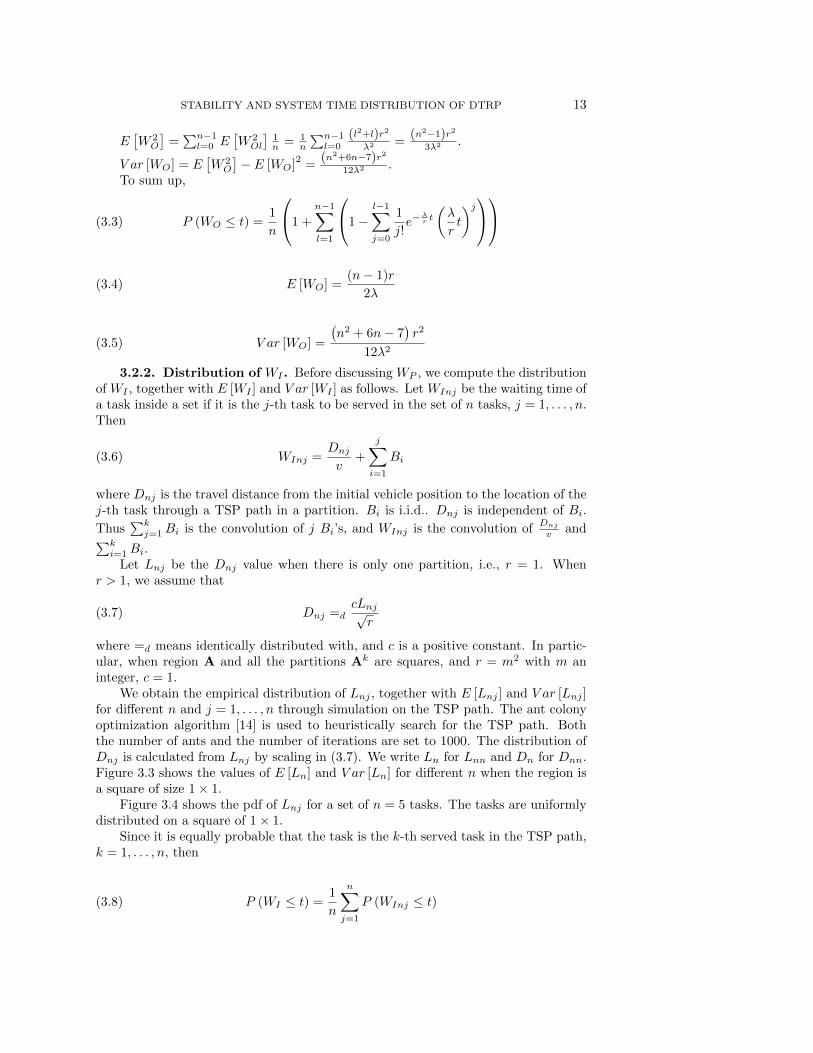
3.2.2. Distribution of WI . Before discussing WP , we compute the distributionof WI , together with E [WI ] and V ar [WI ] as follows. Let WInj be the waiting time ofa task inside a set if it is the j-th task to be served in the set of n tasks, j = 1, . . . , n.Then

WInj =Dnj

v+

j∑i=1

Bi(3.6)

where Dnj is the travel distance from the initial vehicle position to the location of thej-th task through a TSP path in a partition. Bi is i.i.d.. Dnj is independent of Bi.

Thus∑kj=1Bi is the convolution of j Bi’s, and WInj is the convolution of

Dnjv and∑k

i=1Bi.Let Lnj be the Dnj value when there is only one partition, i.e., r = 1. When

r > 1, we assume that

Dnj =dcLnj√r

(3.7)

where =d means identically distributed with, and c is a positive constant. In partic-ular, when region A and all the partitions Ak are squares, and r = m2 with m aninteger, c = 1.

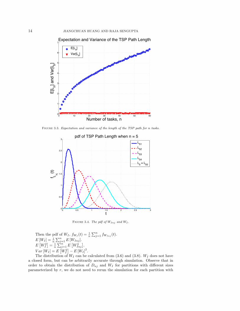
We obtain the empirical distribution of Lnj , together with E [Lnj ] and V ar [Lnj ]for different n and j = 1, . . . , n through simulation on the TSP path. The ant colonyoptimization algorithm [14] is used to heuristically search for the TSP path. Boththe number of ants and the number of iterations are set to 1000. The distribution ofDnj is calculated from Lnj by scaling in (3.7). We write Ln for Lnn and Dn for Dnn.Figure 3.3 shows the values of E [Ln] and V ar [Ln] for different n when the region isa square of size 1× 1.

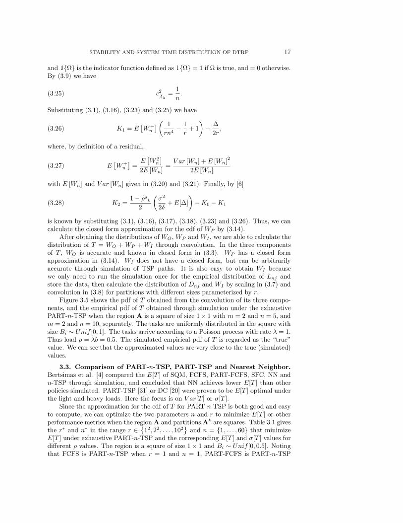
Figure 3.4 shows the pdf of Lnj for a set of n = 5 tasks. The tasks are uniformlydistributed on a square of 1× 1.

Since it is equally probable that the task is the k-th served task in the TSP path,k = 1, . . . , n, then

P (WI ≤ t) =1

n

n∑j=1

P (WInj ≤ t)(3.8)


0 10 20 30 40 50 600

1

2

3

4

5

6

7

Number of tasks, n

E[L n] a

nd V

ar[L n]

Expectation and Variance of the TSP Path Length

E[Ln]

Var[Ln]

Figure 3.3. Expectation and variance of the length of the TSP path for n tasks.

0 0.5 1 1.5 2 2.5 30

0.5

1

1.5

2

2.5

3

t

f L nj(t)

pdf of TSP Path Length when n = 5

L51L52L53L54L5 = L55

Figure 3.4. The pdf of WInj and WI .

Then the pdf of WI , fWI(t) = 1

n

∑nj=1 fWInj

(t).

E [WI ] = 1n

∑nj=1E [WInj ].

E[W 2I

]= 1

n

∑nj=1E

[W 2Inj

].

V ar [WI ] = E[W 2I

]− E [WI ]

2.

The distribution of WI can be calculated from (3.6) and (3.8). WI does not havea closed form, but can be arbitrarily accurate through simulation. Observe that inorder to obtain the distribution of Dnj and WI for partitions with different sizesparameterized by r, we do not need to rerun the simulation for each partition with


different size. We only need to run it once for Lnj and store the data. Dnj and WI

are obtained by scaling and convolution.

3.2.3. Distribution of WP . The analysis of WP uses the results from [15] byestablishing the PART-n-TSP to be equivalent to a classic polling system over jobsthat are the sets N k

l .Since the task arrival process is Poisson with arrival rate λ, the distribution of

the interarrival time of sets, A, is Erlang of order n and arrival rate λ, i.e., A ∼Erlang(n, λ). Let Ak be the interarrival time of sets that fall in partition Ak. ThenAk ∼ Erlang(n, λr ). Thus

E [Ak] =nr

λ, V ar [Ak] =

nr2

λ2(3.9)

The arrival rate of a set is

λs =λ

n(3.10)

The arrival rate of a set in partition Ak, k = 1, . . . , r, is

λsk =λs

r=

λ

nr(3.11)

The size of a set, or the time needed to travel to and execute all the tasks in theset, is WInn as given in (3.6). We write Wn for WInn. The size of each set Wn isi.i.d.. Thus, if we treat each set as a job with size Wn, and each partition as a pollingstation, then the system is a classic polling system on r polling stations with renewal(Erlang) arrival of rate λs, job size Wn, and switch time ∆k. The load is

ρs = λsE [Wn](3.12)

The load in partition Ak, k = 1, . . . , r, is

ρsk =ρs

r(3.13)

WP is the waiting time of each set (job) in this classic polling system. Exhaustiveor gated PART-n-TSP correspond to exhaustive or gated FCFS on sets, respectively.

Dorsman et al. [15] provide closed form approximations for the distribution ofthe steady state waiting time of a job, WP , for polling systems under a renewal arrivalprocess with gated or exhaustive policies when the sequencing policy is FCFS. Theyclaim that for exhaustive-FCFS policies,

P (WP ≤ t) ≈ P (UI ≤ (1− ρs)t)(3.14)

where U is uniformly distributed on [0, 1], and I is Gamma distributed with parame-ters

α =2E[∆]δ

σ2+ 1, β =

2E[∆]δ + σ2

2σ2(1− ρs)E [WBoon].(3.15)

where ∆ =∑rk=1 ∆k is the total switch time in a cycle. When the region A and

partitions Ak are squares as shown in Figure 3.1, ∆ is given in (3.1). ρs is given in(3.12).


To explain δ, σ2 and E [WBoon], we denote by y the value of each variable y thatis a function of ρs evaluated at ρs = 1. δ =

∑rj=1

∑rk=j+1 ρ

sj ρsk, where ρsk is given

in (3.13) evaluated at ρs = 1. Since we have equitable partitions, then

ρsk =1

r(3.16)

for all k = 1, . . . , r. Thus

δ =r(r − 1)

2r2=r − 1

2r.(3.17)

Again by [15]

σ2 =∑rk=1 λ

sk

(V ar [Wn] + ρs

2kV ar

[Ak

]).

Since λ = nλs by (3.11), then V ar[Ak

]= nr2

λ2= r2

nλs2 by (3.9). Also, λsk = λs

r

by (3.11), then substituting (3.16) we have σ2 = λs(V ar [Wn] + 1

r2r2

nλs2

). Thus,

σ2 = λs(V ar [Wn] +

1

nλs2

),(3.18)

where by (3.12)

λs =1

E [Wn].(3.19)

From (3.6) we know

E [Wn] =E [Dn]

v+ nb(3.20)

V ar [Wn] =V ar [Dn]

v2+ nσ2

B(3.21)

where E [Dn] and V ar [Dn] are obtained from E [Ln] and V ar [Ln] by (3.7), and E [Ln]and V ar [Ln] are obtained from simulation as shown in Figure 3.3. Thus σ2 is knownsubstituting (3.19), (3.20) and (3.21).

Finally by Boon et al. [6], for equitable partitions

E [WBoon] =K0 +K1ρ

s +K2 (ρs)2

1− ρs(3.22)

where K0 = E [∆+]. ∆+ is called the residual of the random variable ∆ with E [∆+] =E[∆2]2E[∆] . In our case, ∆ is deterministic. Thus,

K0 = E[∆+]

=∆

2(3.23)

with ∆ given in (3.1). K1 = ρsk

((c2Ak

)4

1c2Ak≤ 1+ 2

c2Ak

c2Ak

+11c2

Ak> 1 − 1

)E [W+

n ]

+ E [W+n ] + ρsk (E [∆+]− E[∆]), where

c2Ak

=V ar

[Ak

]E[Ak

]2 ,(3.24)


and 1Ω is the indicator function defined as 1Ω = 1 if Ω is true, and = 0 otherwise.By (3.9) we have

c2Ak

=1

n.(3.25)

Substituting (3.1), (3.16), (3.23) and (3.25) we have

K1 = E[W+n

]( 1

rn4− 1

r+ 1

)− ∆

2r,(3.26)

where, by definition of a residual,

E[W+n

]=E[W 2n

]2E [Wn]

=V ar [Wn] + E [Wn]

2

2E [Wn](3.27)

with E [Wn] and V ar [Wn] given in (3.20) and (3.21). Finally, by [6]

K2 =1− ρsk

2

(σ2

2δ+ E[∆]

)−K0 −K1(3.28)

is known by substituting (3.1), (3.16), (3.17), (3.18), (3.23) and (3.26). Thus, we cancalculate the closed form approximation for the cdf of WP by (3.14).

After obtaining the distributions of WO, WP and WI , we are able to calculate thedistribution of T = WO + WP + WI through convolution. In the three componentsof T , WO is accurate and known in closed form in (3.3). WP has a closed formapproximation in (3.14). WI does not have a closed form, but can be arbitrarilyaccurate through simulation of TSP paths. It is also easy to obtain WI becausewe only need to run the simulation once for the empirical distribution of Lnj andstore the data, then calculate the distribution of Dnj and WI by scaling in (3.7) andconvolution in (3.8) for partitions with different sizes parameterized by r.

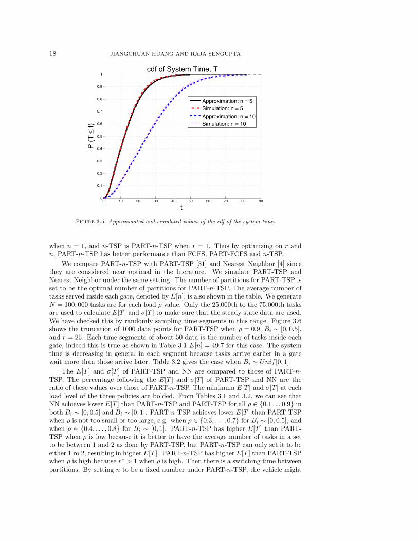
Figure 3.5 shows the pdf of T obtained from the convolution of its three compo-nents, and the empirical pdf of T obtained through simulation under the exhaustivePART-n-TSP when the region A is a square of size 1× 1 with m = 2 and n = 5, andm = 2 and n = 10, separately. The tasks are uniformly distributed in the square withsize Bi ∼ Unif [0, 1]. The tasks arrive according to a Poisson process with rate λ = 1.Thus load ρ = λb = 0.5. The simulated empirical pdf of T is regarded as the “true”value. We can see that the approximated values are very close to the true (simulated)values.

3.3. Comparison of PART-n-TSP, PART-TSP and Nearest Neighbor.Bertsimas et al. [4] compared the E[T ] of SQM, FCFS, PART-FCFS, SFC, NN andn-TSP through simulation, and concluded that NN achieves lower E[T ] than otherpolicies simulated. PART-TSP [31] or DC [20] were proven to be E[T ] optimal underthe light and heavy loads. Here the focus is on V ar[T ] or σ[T ].

Since the approximation for the cdf of T for PART-n-TSP is both good and easyto compute, we can optimize the two parameters n and r to minimize E[T ] or otherperformance metrics when the region A and partitions Ak are squares. Table 3.1 givesthe r∗ and n∗ in the range r ∈

12, 22, . . . , 102

and n = 1, . . . , 60 that minimize

E[T ] under exhaustive PART-n-TSP and the corresponding E[T ] and σ[T ] values fordifferent ρ values. The region is a square of size 1× 1 and Bi ∼ Unif [0, 0.5]. Notingthat FCFS is PART-n-TSP when r = 1 and n = 1, PART-FCFS is PART-n-TSP


0 10 20 30 40 50 60 70 80 900

0.1

0.2

0.3

0.4

0.5

0.6

0.7

0.8

0.9

1

t

P (T

≤ t)

cdf of System Time, T

Approximation: n = 5Simulation: n = 5Approximation: n = 10Simulation: n = 10

Figure 3.5. Approximated and simulated values of the cdf of the system time.

when n = 1, and n-TSP is PART-n-TSP when r = 1. Thus by optimizing on r andn, PART-n-TSP has better performance than FCFS, PART-FCFS and n-TSP.

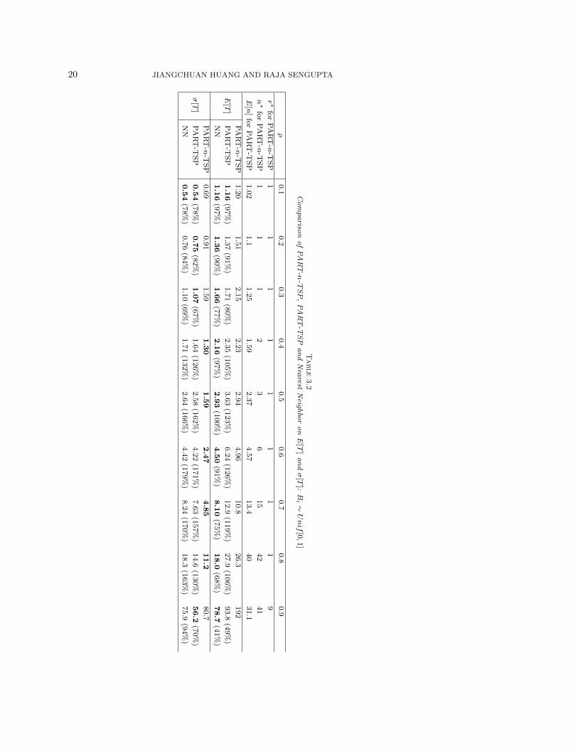
We compare PART-n-TSP with PART-TSP [31] and Nearest Neighbor [4] sincethey are considered near optimal in the literature. We simulate PART-TSP andNearest Neighbor under the same setting. The number of partitions for PART-TSP isset to be the optimal number of partitions for PART-n-TSP. The average number oftasks served inside each gate, denoted by E[n], is also shown in the table. We generateN = 100, 000 tasks are for each load ρ value. Only the 25,000th to the 75,000th tasksare used to calculate E[T ] and σ[T ] to make sure that the steady state data are used.We have checked this by randomly sampling time segments in this range. Figure 3.6shows the truncation of 1000 data points for PART-TSP when ρ = 0.9, Bi ∼ [0, 0.5],and r = 25. Each time segments of about 50 data is the number of tasks inside eachgate, indeed this is true as shown in Table 3.1 E[n] = 49.7 for this case. The systemtime is decreasing in general in each segment because tasks arrive earlier in a gatewait more than those arrive later. Table 3.2 gives the case when Bi ∼ Unif [0, 1].

The E[T ] and σ[T ] of PART-TSP and NN are compared to those of PART-n-TSP, The percentage following the E[T ] and σ[T ] of PART-TSP and NN are theratio of these values over those of PART-n-TSP. The minimum E[T ] and σ[T ] at eachload level of the three policies are bolded. From Tables 3.1 and 3.2, we can see thatNN achieves lower E[T ] than PART-n-TSP and PART-TSP for all ρ ∈ 0.1 . . . 0.9 inboth Bi ∼ [0, 0.5] and Bi ∼ [0, 1]. PART-n-TSP achieves lower E[T ] than PART-TSPwhen ρ is not too small or too large, e.g. when ρ ∈ 0.3, . . . , 0.7 for Bi ∼ [0, 0.5], andwhen ρ ∈ 0.4, . . . , 0.8 for Bi ∼ [0, 1]. PART-n-TSP has higher E[T ] than PART-TSP when ρ is low because it is better to have the average number of tasks in a setto be between 1 and 2 as done by PART-TSP, but PART-n-TSP can only set it to beeither 1 ro 2, resulting in higher E[T ]. PART-n-TSP has higher E[T ] than PART-TSPwhen ρ is high because r∗ > 1 when ρ is high. Then there is a switching time betweenpartitions. By setting n to be a fixed number under PART-n-TSP, the vehicle might


Table3.1

Compa

risonofPART-n

-TSP,PART-T

SP

andNearest

Neigh

boronE

[T]andσ

[T]:B

i∼Unif

[0,0.5

]

ρ0.1

0.2

0.3

0.4

0.5

0.6

0.7

0.8

0.9

r∗

for

PA

RT

-n-T

SP

11

11

11

14

25

n∗

for

PA

RT

-n-T

SP

12

24

12

24

57

59

57

E[n

]fo

rP

AR

T-T

SP

1.0

51.2

51.7

53.4

69.0

823.3

61.2

63.9

49.7

PA

RT

-n-T

SP

1.0

41.7

11.7

02.8

05.9

09.9

920.3

81.4

321

E[T

]P

AR

T-T

SP

0.9

5(9

1%

)1.2

6(7

4%

)1.8

7(1

10%

)3.3

0(1

18%

)5.9

7(1

01%

)10.9

(109%

)24.4

(120%

)51.7

(64%

)181

(56%

)

NN

0.94

(90%

)1.21

(71%

)1.66

(98%

)2.46

(88%

)3.81

(65%

)6.37

(64%

)12.7

(63%

)32.6

(40%

)154

(48%

)

PA

RT

-n-T

SP

0.6

91.1

90.94

1.39

2.74

4.36

8.56

31.7

140

σ[T

]P

AR

T-T

SP

0.4

8(7

0%

)0.7

7(6

5%

)1.2

2(1

30%

)2.1

1(1

52%

)3.2

7(1

19%

)5.3

5(1

23%

)13.3

(155%

)27.1

(85%

)101

(72%

)

NN

0.47

(68%

)0.76

(64%

)1.2

6(1

34%

)2.1

4(1

54%

)3.5

7(1

30%

)6.1

8(1

42%

)12.5

(146%

)31.1

(98%

)147

(105%

)


Table3.2

Compa

risonofPART-n

-TSP,PART-T

SP

andNearest

Neigh

boronE

[T]andσ

[T]:B

i∼Unif

[0,1

]

ρ0.1

0.2

0.3

0.4

0.5

0.6

0.7

0.8

0.9

r ∗fo

rP

AR

T-n

-TS

P1

11

11

11

19

n∗

for

PA

RT

-n-T

SP

11

12

36

15

42

41

E[n

]fo

rP

AR

T-T

SP

1.0

21.1

1.2

51.5

92.3

74.5

713.4

40

31.1

PA

RT

-n-T

SP

1.2

01.5

12.1

52.2

32.9

44.9

610.8

26.3

192

E[T

]P

AR

T-T

SP

1.16

(97%

)1.3

7(9

1%

)1.7

1(8

0%

)2.3

5(1

05%

)3.6

3(1

23%

)6.2

4(1

26%

)12.9

(119%

)27.9

(106%

)93.8

(49%

)

NN

1.16

(97%

)1.36

(90%

)1.66

(77%

)2.16

(97%

)2.93

(100%

)4.50

(91%

)8.10

(75%

)18.0

(68%

)78.7

(41%

)

PA

RT

-n-T

SP

0.6

90.9

11.5

91.30

1.59

2.47

4.85

11.2

80.7

σ[T

]P

AR

T-T

SP

0.54

(78%

)0.75

(82%

)1.07

(67%

)1.6

4(1

26%

)2.5

8(1

62%

)4.2

2(1

71%

)7.6

3(1

57%

)14.6

(130%

)56.2

(70%

)

NN

0.54

(78%

)0.7

6(8

4%

)1.1

0(6

9%

)1.7

1(1

32%

)2.6

4(1

66%

)4.4

2(1

79%

)8.2

4(1

70%

)18.3

(163%

)75.9

(94%

)


0 100 200 300 400 500 600 700 800 900 10000

50

100

150

200

250

300

350

400

Task label

Sim

ulat

ed s

yste

m ti

me,

T

Part of Simulated Data for PART−TSP: ρ = 0.9, Bi ~ [0,0.5], r = 25

Figure 3.6. Part of simulated data for PART-TSP: ρ = 0.9, Bi ∼ [0, 0.5], and r = 25.

arrive at a partition, and find the number of tasks to be less than n. Then the vehiclewould switch to the next partition without serving any task, resulting in a switchingcost but no tasks served.

PART-n-TSP behaves like a “standardized” version of PART-TSP. While thefixed n reduces flexibility, it increases certainty. Thus V ar[T ] or σ[T ] should be lower.Indeed, as shown in Tables 3.1 and 3.2, PART-n-TSP achieves lower σ[T ] than PART-TSP and NN when ρ is not too small or too large, e.g. when ρ ∈ 0.3, . . . , 0.7 forBi ∼ [0, 0.5], and when ρ ∈ 0.4, . . . , 0.8 for Bi ∼ [0, 1]. The performance of PART-n-TSP on σ[T ] when ρ is too small or too large is not as good for the same reasonsaffecting E[T ] as explained in the previous paragraph.

3.4. Optimality of PART-n-TSP under light and heavy loads. The PART-n-TSP can be modified to yield asymptotically optimal E[T ] under light load (ρ →0+). First the PART-n-TSP becomes FCFS policy when setting r = 1 and n = 1.Then under FCFS policy, let the vehicle return to the median of region A when itbecomes idle. Under light load this is the stochastic queue median (SQM) policy [4],where the vehicle travels directly to the task location from the median, executes thetask, and then returns to the median after completion. SQM is proven to be E[T ]optimal under light load [4], proving the optimality of PART-n-TSP under light load.

Under heavy load (ρ→ 1−), the following lower bound holds [5].

E[T ] ≥β2TSP,2λ

(∫Af

12

X(x) dx)2

2v2(1− ρ)2(3.29)

The following theorem shows that PART-n-TSP achieves the heavy-load lowerbound (3.29) when r → ∞. Thus PART-n-TSP is asymptotically optimal in E[T ]under heavy load.

Theorem 3.2. Under PART-n-TSP as per Definition 3.1, when ρ → 1− and


n→∞, the system time for the 1-DTRP satisfies

E[T ] ≤(

1 +1

r

) β2TSP,2λ

(∫Af

12

X(x) dx)2

2v2(1− ρ)2(3.30)

where r is the number of partitions.Proof. E[T ] = E [WO] + E [WP ] + E [WI ] by (3.2).And by (3.4)

E [WO] =(n− 1)r

2λ<nr

2λ(3.31)

By (3.6) and (3.8), and conditioning on the position that a given task takes withinits set, and noting that the travel time around the TSP path is no more than the lengthof the path itself, the expected wait for completion once a task’s set enters service

E [WI ] ≤1

vE [Dn] +

1

n

n∑j=1

jb =1

vE [Dn] +

n+ 1

2b(3.32)

Given that a demand falls in partition Ak, the conditional density for its loca-

tion (whose support is Ak) is fX(x)∫Ak

fX(x) dx. From [24] we know that, almost surely,

limn→∞Dn√n

= βTSP,2∫Ak

√fX(x)∫

AkfX(x) dx

dx, where βTSP,2 is a constant. Let C =

1vβTSP,2

∫Ak

√fX(x)∫

AkfX(x) dx

dx, thus C is a constant. So limn→∞1vE [Dn] = C

√n.

The load of a set ρs = λsE [Wn] = λn

(E[Dn]v + nb

)= λb + λ

vE[Dn]n = ρ +

λE[Dn]nv by (3.11), (3.12) and (3.20). Thus limn→∞ ρs = ρ + λ limn→∞

E[Dn]nv =

ρ+ λ limn→∞C√n

n = ρ. So ρ→ 1− implies ρs → 1− when n→∞.As for E [WP ], from [28] we know that the mean waiting time in a polling system

with renewal arrivals as ρs → 1− is

E [WP ] =ω

1− ρs+ o

((1− ρs)−1

),(3.33)

where ω = 1−ρsk2

(σ2∑r

k=1 ρsk(1−ρsk)

+ E[∆]

)under the exhaustive policy, and ω =

1+ρsk2

(σ2∑r

k=1 ρsk(1+ρsk)

+ E[∆]

)under the gated policy. Substituting (3.16) we have

ω = σ2

2 + r−12r E[∆] under the exhaustive policy, and ω = σ2

2 + r+12r E[∆] under the

gated policy. ∆ =∑rk=1 ∆k is the total switch time of a polling cycle. ∆ does not

depend on ρ, ρs or n, and is given in (3.1) when the region A and partitions Ak aresquares.

Thus E [WP ] = 12(1−ρs)

(σ2 + r∓1

r E[∆])

+ o((1− ρs)−1

)when ρs → 1−. Let

C ′ = r∓1r E[∆]. So E [WP ] = 1

2(1−ρs)(σ2 + C ′

)when ρs → 1−. Since r is a finite

natural number, and ∆k is upper bounded by the diameter of region A, then E[∆] isa positive finite number. Thus, C ′ is a positive finite number.

By (3.18) σ2 = λs(V ar [Wn] + 1

nλs2

), where λs = λ

n by (3.11). Also, ρs =

λsE [Wn] as ρs → 1− by (3.12).


So E [WP ] =λs(V ar[Wn]+ 1

nλs2

)+C′

2(1−λsE[Wn])

=λn ( 1

v2V ar[Dn]+nσ2

B+ nλ2

)+C′

2(

1− λn ( 1vE[Dn]+nb)

)=

λ( 1λ2

+V ar[Dn]

nv2+σ2

B)+C′

2(1−λb−λ 1vE[Dn]n )

, as ρs → 1−, where we substituted λs = λn and (3.20) and

(3.21) in the first equality.

Since λ is the value of λ when ρs = 1, and ρ→ 1− implies ρs → 1−, then we canwrite

E [WP ] =λ(

1λ2 + V ar[Dn]

nv2 + σ2B

)+ C ′

2(

1− ρ− λ 1vE[Dn]n

)(3.34)

when ρ→ 1−, where we substituted ρ = λb.

From [19, p.189] we know limn→∞ V ar [Dn] = O(1), and therefore, limn→∞V ar[Dn]

n =0.

Thus when ρ→ 1− and n→∞,E[T ] = E [WO] + E [WP ] + E [WI ]

≤ (n−1)r2λ + 1

vE [Dn] + n+12 b+

λ( 1λ2

+V ar[Dn]

nv2+σ2

B)+C′

2(1−ρ−λ 1vE[Dn]n )

≤ nr2λ + C

√n+ n

2 b+λ( 1

λ2+σ2

B)+C′

2(

1−ρ−λ C√n

) .

Substituting b = ρλ we have

E[T ] ≤λ(

1λ2 + σ2

B

)+ C ′

2(

1− ρ− λ C√n

) +n(r + ρ)

2λ+ C√n(3.35)

We want to minimize (3.35) with respect to n to get the least upper bound.Noting that (3.35) is convex with respect to n, so there is indeed a minimum. First,however, consider a change of variable y = λC

(1−ρ)√n

. With this change,

E[T ] ≤λ(

1λ2 + σ2

B

)+ C ′

2(1− ρ)(1− y)+λC2(r + ρ)

2(1− ρ)2y2+

λC2

(1− ρ)y(3.36)

For ρ → 1−, one can verify that the optimum y approaches 1. Linearizing the

last two terms above about y = 1 we have λC2(r+ρ)2(1−ρ)2y2 = λC2(r+ρ)

2(1−ρ)2 (3−2y), and λC2

(1−ρ)y =λC2

1−ρ (2− y).

Thus, g(y) ≡ λ( 1λ2

+σ2B)+C′

2(1−ρ)(1−y) + λC2(r+ρ)2(1−ρ)2y2 + λC2

(1−ρ)y≈ C1

1−y + C2(3− 2y) + C3(2− y)

= C1

1−y + (2C2 + C3) (1− y) +C2 +C3, where C1 =λ( 1

λ2+σ2

B)+C′

2(1−ρ) , C2 = λC2(r+ρ)2(1−ρ)2 , and

C3 = λC2

1−ρ .

The approximation for g(y) is minimized when C1

1−y = (2C2 + C3) (1 − y). Sub-stituting C1, C2 and C3 we have an approximate optimum value

y∗ = 1− 1

C

√(1λ2 + σ2

B + C′

λ

)(1− ρ)

2(1 + r)(3.37)


Substituting (3.37) into (3.36) and noting that for ρ → 1− the approximate y∗

approaches 1 we have

E[T ] ≤ λC2(r + 1)

2(1− ρ)2+λC√

2(r + 1)(

1λ2 + σ2

B + C′

λ

)2(1− ρ)

32

+λC2

1− ρ(3.38)

when ρ→ 1−.

Thus E[T ] ≤ λC2(r+1)2(1−ρ)2 + o

((1− ρ)−2

)when ρ→ 1−. We have

E[T ] ≤ λC2(r + 1)

2(1− ρ)2(3.39)

when ρ→ 1−.

C = 1vβTSP,2

∫Ak

√fX(x)∫

AkfX(x) dx

dx

= 1vβTSP,2

√r∫Ak

√fX(x) dx

= βTSP,21

v√r

∫A

√fX(x) dx.

Substituting C in (3.39) we have

E[T ] ≤(

1 +1

r

) β2TSP,2λ

(∫Af

12

X(x) dx)2

2v2(1− ρ)2.

The PART-n-TSP is optimal under light load. Moreover, when r → ∞, thePART-n-TSP policy achieves the heavy-load lower bound (3.29). Therefore thePART-n-TSP is both optimal under light load and arbitrarily close to optimalityunder heavy load, and stabilizes the system for every load ρ ∈ [0, 1). Notice thatwith r = 10 the PART-n-TSP is already guaranteed to be within 10% of the optimalperformance under heavy load.

4. Summary. We give a good approximation for the distribution of the systemtime that is easy to compute under the PART-n-TSP policy by utilizing the approx-imation results of the distribution of system time T , together with E[T ] and V ar[T ]in the polling systems [8, 15]. We compare PART-n-TSP with PART-TSP [31] andNearest Neighbor [4] on E[T ] and σ[T ] in Tables 3.1 and 3.2, since the latter two areconsidered near optimal in the literature. The results show that in practice PART-n-TSP achieves lower σ[T ] than PART-TSP and NN and lower E[T ] than PART-TSPwhen the load ρ is not too small or too large. We also prove that PART-n-TSP isE[T ] optimal under light load (ρ→ 0+) and asymptotically optimal under heavy load(ρ→ 1−) in Theorem 3.2.

5. Conclusion. We prove a necessary and sufficient condition for stability inthe Dynamic Traveling Repairman Problem (DTRP) [4] under the class of Polling-Sequencing (P-S) policies satisfying unlimited-polling and economy of scale. Thenumber of tasks inside each polling partition is shown to be a Markov chain. Non-location based policies and some common location based policies such as TSP, NN andDA are shown to have economy of scale. The P-S class includes some of the policiesproven to be optimal for the expectation of system time under light and heavy loadsin the DTRP literature. We give a close form approximation of the distribution of thesteady state system time, together with its expectation and variance for PART-n-TSP


policy in the P-S class, which is proved to be optimal for the expectation of systemtime under light and heavy loads.

REFERENCES

[1] Eitan Altman, Panagiotis Konstantopoulos, and Zhen Liu. Stability, monotonicity and invariantquantities in general polling systems. Queueing Systems, 11:35–57, 1992.

[2] Dragomir Anguelov, Carole Dulong, Daniel Filip, Christian Frueh, Stphane Lafon, RichardLyon, Abhijit Ogale, Luc Vincent, and Josh Weaver. Google street view: Capturing theworld at street level. Computer, 43, 2010.

[3] S. Asmussen. Applied Probability and Queues. Applications of Mathematics. Springer, 2003.[4] Dimitris J Bertsimas and Garrett Van Ryzin. A stochastic and dynamic vehicle routing problem

in the euclidean plane. Operations Research, 39(4):601–615, 1991.[5] Dimitris J Bertsimas and Garrett Van Ryzin. Stochastic and dynamic vehicle routing with

general demand and interarrival time distributions. Advances in Applied Probability, pages947–978, 1993.

[6] M. A. A. Boon, E. M. M. Winands, I. J. B. F. Adan, and A. C. C. van Wijk. Closed-formwaiting time approximations for polling systems. Perform. Eval., 68(3):290–306, March2011.

[7] A.A. Borovkov and R. Schassberger. Ergodicity of a polling network. Stochastic Processes andtheir Applications, 50(2):253 – 262, 1994.

[8] Onno Boxma, Josine Bruin, and Brian Fralix. Sojourn times in polling systems with variousservice disciplines. Performance Evaluation, 66(11):621 – 639, 2009.

[9] J.W. Cohen. The single server queue. North-Holland series in applied mathematics and me-chanics. North-Holland Pub. Co., 1982.

[10] Carlos F. Daganzo. An approximate analytic model of many-to-many demand responsive trans-portation systems. Transportation Research, 12(5):325 – 333, 1978.

[11] Carlos F. Daganzo. The length of tours in zones of different shapes. Transportation ResearchPart B: Methodological, 18(2):135 – 145, 1984.

[12] Prabuddha De, Jay B. Ghosh, and Charles E. Wells. Expectation-variance analyss of jobsequences under processing time uncertainty. International Journal of Production Eco-nomics, 28(3):289 – 297, 1992.

[13] Benedict G. C. Dellaert and Barbara E. Kahn. How tolerable is delay? consumers’ evaluationsof internet web sites after waiting. Journal of Interactive Marketing, 13:41–54, 1999.

[14] Marco Dorigo and Luca Maria Gambardella. Ant colonies for the travelling salesman problem.Biosystems, 43(2):73 – 81, 1997.

[15] J. L. Dorsman, R. D. van der Mei, and E. M. M. Winands. A new method for deriving Waiting-Time approximations in polling systems with renewal arrivals. Stochastic Models, 27:318– 332, 2011.

[16] C. Fricker and M.R. Jaibi. Monotonicity and stability of periodic polling models. QueueingSystems, 15:211–238, 1994.

[17] Michael K. Hui and Lianxi Zhou. How does waiting duration information influence customers’reactions to waiting for services?1. Journal of Applied Social Psychology, 26(19):1702–1717,1996.

[18] Karen Jenvey. NASA Unmanned Aircraft Measures Low Altitude Greenhouse Gases, December2011.

[19] Eugene Lawler. The Traveling Salesman Problem: A Guided Tour of Combinatorial Optimiza-tion. Wiley, New York, 1985.

[20] M. Pavone, E. Frazzoli, and F. Bullo. Adaptive and distributed algorithms for vehicle routingin a stochastic and dynamic environment. Automatic Control, IEEE Transactions on,56(6):1259–1274, June 2011.

[21] Zvi Rosberg. A positive recurrence criterion associated with multidimensional queueing pro-cesses. Journal of Applied Probability, pages 790–801, 1980.

[22] Subhash Sarin, Balaji Nagarajan, Sanjay Jain, and Lingrui Liao. Analytic evaluation of the ex-pectation and variance of different performance measures of a schedule on a single machineunder processing time variability. Journal of Combinatorial Optimization, 17:400–416,2009.

[23] Arun A. Somasundara, Aditya Ramamoorthy, and Mani B. Srivastava. Mobile element schedul-ing for efficient data collection in wireless sensor networks with dynamic deadlines. In Pro-ceedings of the 25th IEEE International Real-Time Systems Symposium, RTSS ’04, pages296–305, Washington, DC, USA, 2004.


[24] J. Michael Steele. Probabilistic and worst case analyses of classical problems of combinatorialoptimization in euclidean space. Math. Oper. Res., 15:749–770, October 1990.

[25] H. Takagi. Analysis of polling systems. MIT Press series in computer systems. MIT Press,1986.

[26] H. Takagi. Queueing analysis: a foundation of performance evaluation, vol. 1 : vacation andpriority systems. Queueing Analysis. North-Holland, 1991.

[27] H. Takagi. Queueing analysis of polling models: progress in 1990-1994. Frontiers in Queueing,pages 119–146, 1997.

[28] R. D. Van Der Mei and E. M. M. Winands. A note on polling models with renewal arrivalsand nonzero switch-over times. Oper. Res. Lett., 36(4):500–505, July 2008.

[29] V. Vishnevskii and O. Semenova. Mathematical methods to study the polling systems. Au-tomation and Remote Control, 67:173–220, 2006.

[30] Adam Wierman. Scheduling for today’s computer systems: bridging theory and practice. PhDthesis, Pittsburgh, PA, USA, 2007.

[31] H. Xu. Optimal policies for stochastic and dynamic vehicle routing problems. Cambridge, 1994.

stability and system time distribution of dynamiccpcc.berkeley.edu/papers/dtrp.pdf · stability and...

Documents