stability of minkowski space for the massless … filestability of minkowski space for the massless...
TRANSCRIPT
Stability of Minkowski Space for the MasslessEinstein–Vlasov System
Martin Taylor
DPMMS, Cambridge
Mathematical General Relativity SeminarInstitut Henri Poincare
7th October 2015
Martin Taylor (Cambridge) Stability of Minkowski Space 7th October 2015 1 / 26
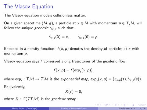
The Vlasov Equation
The Vlasov equation models collisionless matter.
On a given spacetime (M, g), a particle at x ∈ M with momentum p ∈ TxM, willfollow the unique geodesic γx,p such that
γx,p(0) = x , γx,p(0) = p.
Encoded in a density function: f (x , p) denotes the density of particles at x withmomentum p.
Vlasov equation says f conserved along trajectories of the geodesic flow:
f (x , p) = f (exps(x , p)),
where exps : TM→ TM is the exponential map, exps(x , p) = (γx,p(s), γx,p(s)).
Equivalently,X (f ) = 0,
where X ∈ Γ(TTM) is the geodesic spray.
Martin Taylor (Cambridge) Stability of Minkowski Space 7th October 2015 2 / 26
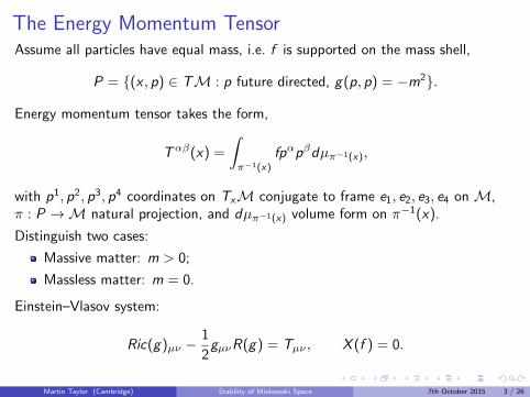
The Energy Momentum TensorAssume all particles have equal mass, i.e. f is supported on the mass shell,
P = {(x , p) ∈ TM : p future directed, g(p, p) = −m2}.
Energy momentum tensor takes the form,
Tαβ(x) =
∫π−1(x)
fpαpβdµπ−1(x),
with p1, p2, p3, p4 coordinates on TxM conjugate to frame e1, e2, e3, e4 on M,π : P →M natural projection, and dµπ−1(x) volume form on π−1(x).
Distinguish two cases:
Massive matter: m > 0;
Massless matter: m = 0.
Einstein–Vlasov system:
Ric(g)µν −1
2gµνR(g) = Tµν , X (f ) = 0.
Martin Taylor (Cambridge) Stability of Minkowski Space 7th October 2015 3 / 26
Stability of Minkowski Space with Massless CollisionlessMatter
The Einstein–Vlasov system has a well posed Cauchy problem and domain ofdependence property (Choquet-Bruhat 1971).
Allows us to pose the question of stability of Minkowski space:
Given an initial data set which is close to that of Minkowski space, whatproperties does the resulting spacetime have?
Theorem (M.T. 2015)
Given regular initial data for the massless Einstein–Vlasov system suitably “close”to that of Minkowski space with f0 compactly supported, the resulting spacetimeis geodesically complete and approaches Minkowski space in every direction.Moreover, the spacetime possesses a complete future null infinity whose causalpast is M.
Martin Taylor (Cambridge) Stability of Minkowski Space 7th October 2015 4 / 26
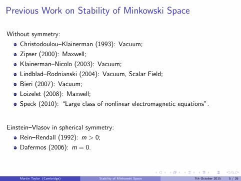
Previous Work on Stability of Minkowski Space
Without symmetry:
Christodoulou–Klainerman (1993): Vacuum;
Zipser (2000): Maxwell;
Klainerman–Nicolo (2003): Vacuum;
Lindblad–Rodnianski (2004): Vacuum, Scalar Field;
Bieri (2007): Vacuum;
Loizelet (2008): Maxwell;
Speck (2010): “Large class of nonlinear electromagnetic equations”.
Einstein–Vlasov in spherical symmetry:
Rein–Rendall (1992): m > 0;
Dafermos (2006): m = 0.
Martin Taylor (Cambridge) Stability of Minkowski Space 7th October 2015 5 / 26
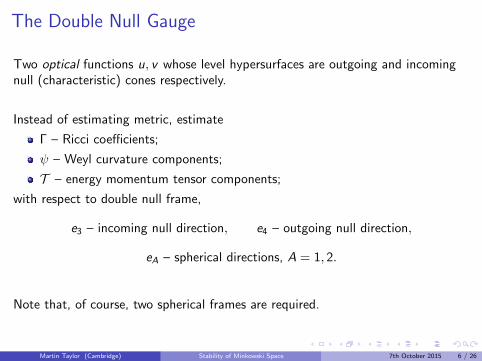
The Double Null Gauge
Two optical functions u, v whose level hypersurfaces are outgoing and incomingnull (characteristic) cones respectively.
Instead of estimating metric, estimate
Γ – Ricci coefficients;
ψ – Weyl curvature components;
T – energy momentum tensor components;
with respect to double null frame,
e3 – incoming null direction, e4 – outgoing null direction,
eA – spherical directions, A = 1, 2.
Note that, of course, two spherical frames are required.
Martin Taylor (Cambridge) Stability of Minkowski Space 7th October 2015 6 / 26
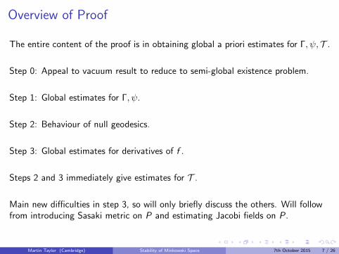
Overview of Proof
The entire content of the proof is in obtaining global a priori estimates for Γ, ψ, T .
Step 0: Appeal to vacuum result to reduce to semi-global existence problem.
Step 1: Global estimates for Γ, ψ.
Step 2: Behaviour of null geodesics.
Step 3: Global estimates for derivatives of f .
Steps 2 and 3 immediately give estimates for T .
Main new difficulties in step 3, so will only briefly discuss the others. Will followfrom introducing Sasaki metric on P and estimating Jacobi fields on P.
Martin Taylor (Cambridge) Stability of Minkowski Space 7th October 2015 7 / 26
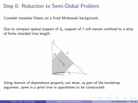
Step 0: Reduction to Semi-Global Problem
Consider massless Vlasov on a fixed Minkowski background.
Due to compact spatial support of f0, support of f will remain confined to a stripof finite retarded time length.
Using domain of dependence property can show, as part of the bootstrapargument, same is a priori true in spacetimes to be constructed.
Martin Taylor (Cambridge) Stability of Minkowski Space 7th October 2015 8 / 26
Step 1: Null Structure and Bianchi Equations
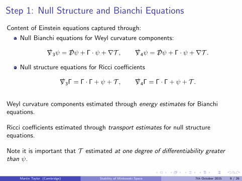
Content of Einstein equations captured through:
Null Bianchi equations for Weyl curvature components:
/∇3ψ = /Dψ + Γ · ψ +∇T , /∇4ψ = /Dψ + Γ · ψ +∇T .
Null structure equations for Ricci coefficients
/∇3Γ = Γ · Γ + ψ + T , /∇4Γ = Γ · Γ + ψ + T .
Weyl curvature components estimated through energy estimates for Bianchiequations.
Ricci coefficients estimated through transport estimates for null structureequations.
Note it is important that T estimated at one degree of differentiability greaterthan ψ.
Martin Taylor (Cambridge) Stability of Minkowski Space 7th October 2015 9 / 26
Global Decay Estimates
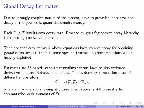
Due to strongly coupled nature of the system, have to prove boundedness anddecay of the geometric quantities simultaneously.
Each Γ, ψ, T has its own decay rate. Proceed by guessing correct decay hierarchythen proving guesses are correct.
Then see that error terms in above equations have correct decay for obtainingglobal estimates, i.e. there is some special structure in above equations which isheavily exploited.
Estimates are L2 based, so to treat nonlinear terms have to also estimatederivatives and use Sobolev inequalities. This is done by introducing a set ofdifferential operators
D = {r /∇, /∇3, r /∇4},
where r = v − u and showing structure in equations is still present aftercommutation with elements of D.
Martin Taylor (Cambridge) Stability of Minkowski Space 7th October 2015 10 / 26
Step 2: Geometry of Null Geodesics
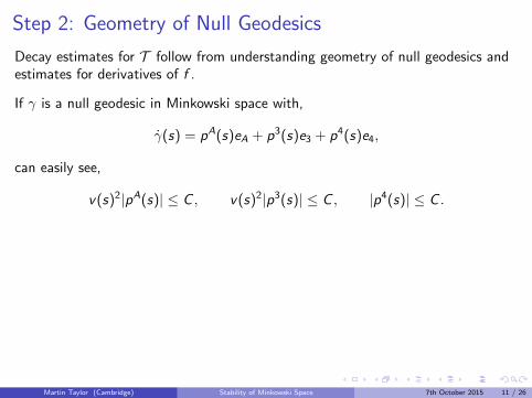
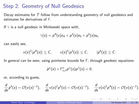
Decay estimates for T follow from understanding geometry of null geodesics andestimates for derivatives of f .
If γ is a null geodesic in Minkowski space with,
γ(s) = pA(s)eA + p3(s)e3 + p4(s)e4,
can easily see,
v(s)2|pA(s)| ≤ C , v(s)2|p3(s)| ≤ C , |p4(s)| ≤ C .
In general can be seen, using pointwise bounds for Γ, through geodesic equations:
pµ(s) + Γµαβpα(s)pβ(s) = 0,
or, according to guess,
d
dsp4(s) = O(v(s)−2),
d
dsv(s)2p3(s) = O(v(s)−2),
d
dsv(s)2pA(s) = O(v(s)−2).
Martin Taylor (Cambridge) Stability of Minkowski Space 7th October 2015 11 / 26
Step 2: Geometry of Null Geodesics
Decay estimates for T follow from understanding geometry of null geodesics andestimates for derivatives of f .
If γ is a null geodesic in Minkowski space with,
γ(s) = pA(s)eA + p3(s)e3 + p4(s)e4,
can easily see,
v(s)2|pA(s)| ≤ C , v(s)2|p3(s)| ≤ C , |p4(s)| ≤ C .
In general can be seen, using pointwise bounds for Γ, through geodesic equations:
pµ(s) + Γµαβpα(s)pβ(s) = 0,
or, according to guess,
d
dsp4(s) = O(v(s)−2),
d
dsv(s)2p3(s) = O(v(s)−2),
d
dsv(s)2pA(s) = O(v(s)−2).
Martin Taylor (Cambridge) Stability of Minkowski Space 7th October 2015 11 / 26
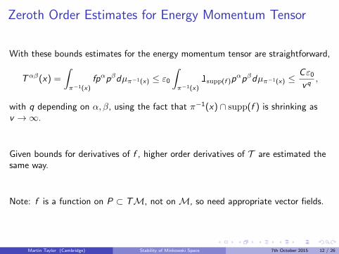
Zeroth Order Estimates for Energy Momentum Tensor
With these bounds estimates for the energy momentum tensor are straightforward,
Tαβ(x) =
∫π−1(x)
fpαpβdµπ−1(x) ≤ ε0∫π−1(x)
1supp(f )pαpβdµπ−1(x) ≤
Cε0vq
,
with q depending on α, β, using the fact that π−1(x) ∩ supp(f ) is shrinking asv →∞.
Given bounds for derivatives of f , higher order derivatives of T are estimated thesame way.
Note: f is a function on P ⊂ TM, not on M, so need appropriate vector fields.
Martin Taylor (Cambridge) Stability of Minkowski Space 7th October 2015 12 / 26
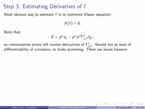
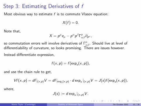
Step 3: Estimating Derivatives of f
Most obvious way to estimate f is to commute Vlasov equation:
X (f ) = 0.
Note that,X = pµeµ − pαpβΓµαβ∂pµ ,
so commutation errors will involve derivatives of Γµαβ . Should live at level ofdifferentiability of curvature, so looks promising. There are issues however.
Instead differentiate expression,
f (x , p) = f (exps(x , p)),
and use the chain rule to get,
Vf (x , p) = df |(x,p)V = df |exps (x,p) · d exps |(x,p)V = J(s)f (exps(x , p)),
where,J(s) := d exps |(x,p)V .
Martin Taylor (Cambridge) Stability of Minkowski Space 7th October 2015 13 / 26
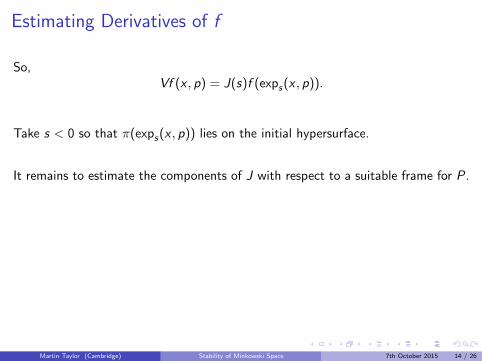
Estimating Derivatives of f
So,Vf (x , p) = J(s)f (exps(x , p)).
Take s < 0 so that π(exps(x , p)) lies on the initial hypersurface.
It remains to estimate the components of J with respect to a suitable frame for P.
When P is given the induced Sasaki metric, J is a Jacobi field alongs 7→ exps(x , p),
∇X ∇X J = R(X , J)X .
Choice of vectors V are important. Will return to this.
Martin Taylor (Cambridge) Stability of Minkowski Space 7th October 2015 14 / 26
Horizontal and Vertical Lifts
Sasaki metric defined using two geometrically defined maps
Hor(x,p),Ver(x,p) : TxM→ T(x,p)TM.
In components, if V = V µeµ,
Ver(x,p)(V ) = V µ∂pµ , Hor(x,p)(V ) = V µeµ − V αpβΓµαβ∂pµ .
Can split T(x,p)TM into direct sum of vertical and horizontal subspaces,
T(x,p)TM = V(x,p) ⊕H(x,p),
V(x,p) = {Ver(x,p)(V ) | V ∈ TxM}, H(x,p) = {Hor(x,p)(V ) | V ∈ TxM}.
For Y ∈ T(x,p)TM, define Y v ,Y h so that,
Y = Ver(x,p)(Y v ) + Hor(x,p)(Y h).
Martin Taylor (Cambridge) Stability of Minkowski Space 7th October 2015 15 / 26
Curvature of the Mass Shell
Recall,∇X ∇X J = R(X , J)X .
Can compute,
R(X , J)X = Hor(γ,γ)
(R(γ, Jh)γ +
3
4R(γ,R(γ, Jh)γ)γ +
1
2(∇γR)(γ, Jv )γ
)+
1
2TVer(γ,γ)
((∇γR)(γ, Jh)γ +
1
2R(γ,R(γ, Jv )γ)γ
),
where (γ(s), γ(s)) = exps(x , p).
Note the derivatives are in the “correct” direction.
Can then compute R in terms of ψ, T . . .
Martin Taylor (Cambridge) Stability of Minkowski Space 7th October 2015 16 / 26
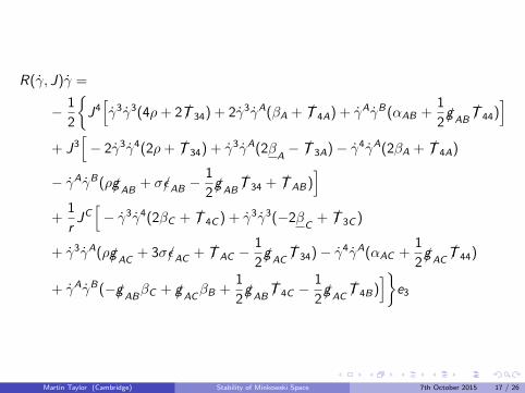
R(γ, J)γ =
− 1
2
{J4[γ3γ3(4ρ+ 2 /T 34) + 2γ3γA(βA + /T 4A) + γAγB(αAB +
1
2/gAB
/T 44)]
+ J3[− 2γ3γ4(2ρ+ /T 34) + γ3γA(2β
A− /T 3A)− γ4γA(2βA + /T 4A)
− γAγB(ρ/gAB+ σ/εAB −
1
2/gAB
/T 34 + /TAB)]
+1
rJC[− γ3γ4(2βC + /T 4C ) + γ3γ3(−2β
C+ /T 3C )
+ γ3γA(ρ/gAC+ 3σ/εAC + /TAC −
1
2/gAC
/T 34)− γ4γA(αAC +1
2/gAC
/T 44)
+ γAγB(−/gABβC + /gAC
βB +1
2/gAB
/T 4C −1
2/gAC
/T 4B)]}
e3
Martin Taylor (Cambridge) Stability of Minkowski Space 7th October 2015 17 / 26
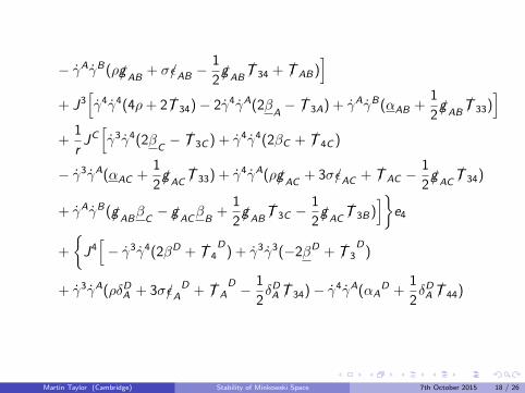
− γAγB(ρ/gAB+ σ/εAB −
1
2/gAB
/T 34 + /TAB)]
+ J3[γ4γ4(4ρ+ 2 /T 34)− 2γ4γA(2β
A− /T 3A) + γAγB(αAB +
1
2/gAB
/T 33)]
+1
rJC[γ3γ4(2β
C− /T 3C ) + γ4γ4(2βC + /T 4C )
− γ3γA(αAC +1
2/gAC
/T 33) + γ4γA(ρ/gAC+ 3σ/εAC + /TAC −
1
2/gAC
/T 34)
+ γAγB(/gABβC− /gAC
βB
+1
2/gAB
/T 3C −1
2/gAC
/T 3B)]}
e4
+
{J4[− γ3γ4(2βD + /T 4
D) + γ3γ3(−2βD + /T 3
D)
+ γ3γA(ρδDA + 3σ/εAD + /TA
D − 1
2δDA /T 34)− γ4γA(αA
D +1
2δDA /T 44)
Martin Taylor (Cambridge) Stability of Minkowski Space 7th October 2015 18 / 26
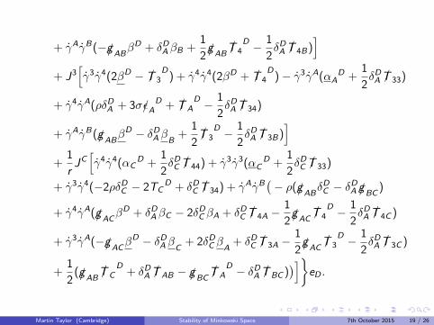
+ γAγB(−/gABβD + δDA βB +
1
2/gAB
/T 4D − 1
2δDA /T 4B)
]+ J3
[γ3γ4(2βD − /T 3
D) + γ4γ4(2βD + /T 4
D)− γ3γA(αA
D +1
2δDA /T 33)
+ γ4γA(ρδDA + 3σ/εAD + /TA
D − 1
2δDA /T 34)
+ γAγB(/gABβD − δDA βB
+1
2/T 3
D − 1
2δDA /T 3B)
]+
1
rJC[γ4γ4(αC
D +1
2δDC /T 44) + γ3γ3(αC
D +1
2δDC /T 33)
+ γ3γ4(−2ρδDC − 2TCD + δDC /T 34) + γAγB
(− ρ(/gAB
δDC − δDA /gBC)
+ γ4γA(/gACβD + δDA βC − 2δDC βA + δDC /T 4A −
1
2/gAC
/T 4D − 1
2δDA /T 4C )
+ γ3γA(−/gACβD − δDA βC
+ 2δDC βA+ δDC /T 3A −
1
2/gAC
/T 3D − 1
2δDA /T 3C )
+1
2(/gAB
/TCD
+ δDA /TAB − /gBC/TA
D − δDA /TBC ))]}
eD .
Martin Taylor (Cambridge) Stability of Minkowski Space 7th October 2015 19 / 26
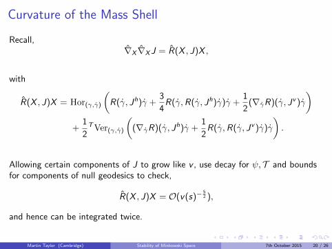
Curvature of the Mass Shell
Recall,∇X ∇X J = R(X , J)X ,
with
R(X , J)X = Hor(γ,γ)
(R(γ, Jh)γ +
3
4R(γ,R(γ, Jh)γ)γ +
1
2(∇γR)(γ, Jv )γ
)+
1
2TVer(γ,γ)
((∇γR)(γ, Jh)γ +
1
2R(γ,R(γ, Jv )γ)γ
).
Allowing certain components of J to grow like v , use decay for ψ, T and boundsfor components of null geodesics to check,
R(X , J)X = O(v(s)−52 ),
and hence can be integrated twice.
Martin Taylor (Cambridge) Stability of Minkowski Space 7th October 2015 20 / 26
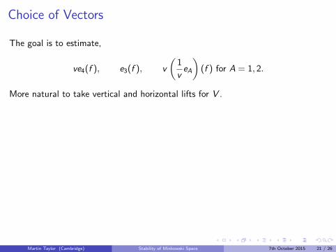
Choice of Vectors
The goal is to estimate,
ve4(f ), e3(f ), v
(1
veA
)(f ) for A = 1, 2.
More natural to take vertical and horizontal lifts for V .
In uncoupled problem in Minkowski space, since J(0) = V ,∇X J(0) = Hor(x,p)(V v ),
J(s) = Par(γ,γ),s(V + sHor(x,p)(V v )
).
RecallVf (x , p) = J(s)f (exps(x , p)),
so just need to control components of J.
Martin Taylor (Cambridge) Stability of Minkowski Space 7th October 2015 21 / 26
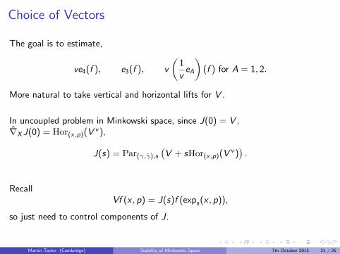
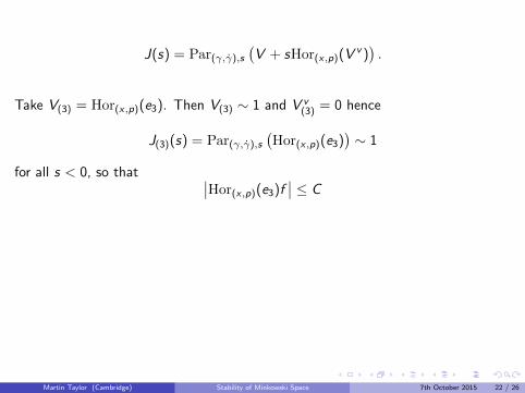
J(s) = Par(γ,γ),s(V + sHor(x,p)(V v )
).
Take V(3) = Hor(x,p)(e3). Then V(3) ∼ 1 and V v(3) = 0 hence
J(3)(s) = Par(γ,γ),s(Hor(x,p)(e3)
)∼ 1
for all s < 0, so that ∣∣Hor(x,p)(e3)f∣∣ ≤ C
Choosing V(A) = vHor(x,p)(1v eA)
for A = 1, 2, again have V v(A) = 0, but now
V(A) ∼ v . So only obtain ∣∣∣∣vHor(x,p)( 1
veA
)∣∣∣∣ ≤ Cv .
Martin Taylor (Cambridge) Stability of Minkowski Space 7th October 2015 22 / 26
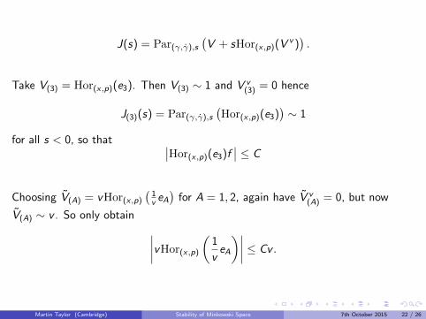
J(s) = Par(γ,γ),s(V + sHor(x,p)(V v )
).
Take V(3) = Hor(x,p)(e3). Then V(3) ∼ 1 and V v(3) = 0 hence
J(3)(s) = Par(γ,γ),s(Hor(x,p)(e3)
)∼ 1
for all s < 0, so that ∣∣Hor(x,p)(e3)f∣∣ ≤ C
Choosing V(A) = vHor(x,p)(1v eA)
for A = 1, 2, again have V v(A) = 0, but now
V(A) ∼ v . So only obtain ∣∣∣∣vHor(x,p)
(1
veA
)∣∣∣∣ ≤ Cv .
Martin Taylor (Cambridge) Stability of Minkowski Space 7th October 2015 22 / 26
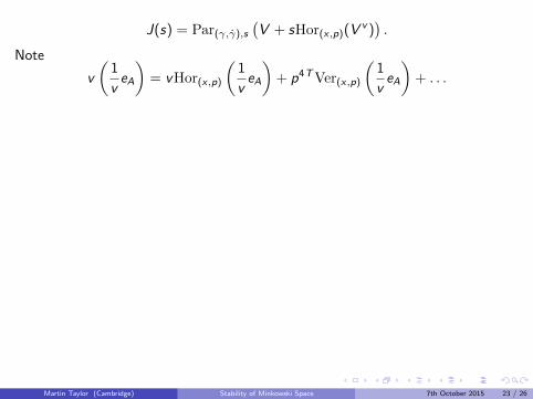
J(s) = Par(γ,γ),s(V + sHor(x,p)(V v )
).
Note
v
(1
veA
)= vHor(x,p)
(1
veA
)+ p4TVer(x,p)
(1
veA
)+ . . .
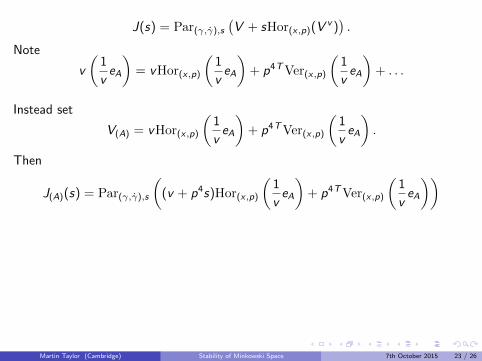
Instead set
V(A) = vHor(x,p)
(1
veA
)+ p4TVer(x,p)
(1
veA
).
Then
J(A)(s) = Par(γ,γ),s
((v + p4s)Hor(x,p)
(1
veA
)+ p4TVer(x,p)
(1
veA
))
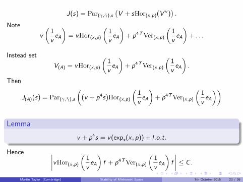
Lemma
v + p4s = v(exps(x , p)) + l .o.t.
Hence ∣∣∣∣vHor(x,p)( 1
veA
)f + p4TVer(x,p)
(1
veA
)f
∣∣∣∣ ≤ C .
Martin Taylor (Cambridge) Stability of Minkowski Space 7th October 2015 23 / 26
J(s) = Par(γ,γ),s(V + sHor(x,p)(V v )
).
Note
v
(1
veA
)= vHor(x,p)
(1
veA
)+ p4TVer(x,p)
(1
veA
)+ . . .
Instead set
V(A) = vHor(x,p)
(1
veA
)+ p4TVer(x,p)
(1
veA
).
Then
J(A)(s) = Par(γ,γ),s
((v + p4s)Hor(x,p)
(1
veA
)+ p4TVer(x,p)
(1
veA
))
Lemma
v + p4s = v(exps(x , p)) + l .o.t.
Hence ∣∣∣∣vHor(x,p)( 1
veA
)f + p4TVer(x,p)
(1
veA
)f
∣∣∣∣ ≤ C .
Martin Taylor (Cambridge) Stability of Minkowski Space 7th October 2015 23 / 26
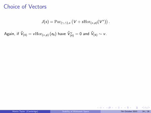
Choice of Vectors
J(s) = Par(γ,γ),s(V + sHor(x,p)(V v )
).
Again, if V(4) = vHor(x,p) (e4) have V v(4) = 0 and V(4) ∼ v .
Instead write
vHor(x,p)(e4) =v
p4X − v2pA
p4Hor(x,p)
(1
veA
)− vp3
p4Hor(x,p)(e3),
and recall that ∣∣∣∣v2pA
p4
∣∣∣∣ , ∣∣∣∣vp3
p4
∣∣∣∣ ≤ C .
So vHor(x,p)(e4) = vp4 X +O(1) and∣∣vHor(x,p)(e4)f
∣∣ ≤ C .
Martin Taylor (Cambridge) Stability of Minkowski Space 7th October 2015 24 / 26
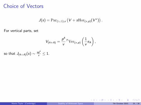
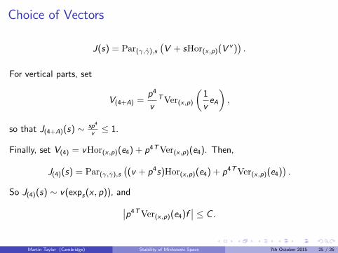
Choice of Vectors
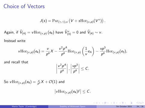
J(s) = Par(γ,γ),s(V + sHor(x,p)(V v )
).
For vertical parts, set
V(4+A) =p4
vTVer(x,p)
(1
veA
),
so that J(4+A)(s) ∼ sp4
v ≤ 1.
Finally, set V(4) = vHor(x,p)(e4) + p4TVer(x,p)(e4). Then,
J(4)(s) = Par(γ,γ),s((v + p4s)Hor(x,p)(e4) + p4TVer(x,p)(e4)
).
So J(4)(s) ∼ v(exps(x , p)), and∣∣p4TVer(x,p)(e4)f∣∣ ≤ C .
Martin Taylor (Cambridge) Stability of Minkowski Space 7th October 2015 25 / 26
Choice of Vectors
J(s) = Par(γ,γ),s(V + sHor(x,p)(V v )
).
For vertical parts, set
V(4+A) =p4
vTVer(x,p)
(1
veA
),
so that J(4+A)(s) ∼ sp4
v ≤ 1.
Finally, set V(4) = vHor(x,p)(e4) + p4TVer(x,p)(e4). Then,
J(4)(s) = Par(γ,γ),s((v + p4s)Hor(x,p)(e4) + p4TVer(x,p)(e4)
).
So J(4)(s) ∼ v(exps(x , p)), and∣∣p4TVer(x,p)(e4)f∣∣ ≤ C .
Martin Taylor (Cambridge) Stability of Minkowski Space 7th October 2015 25 / 26
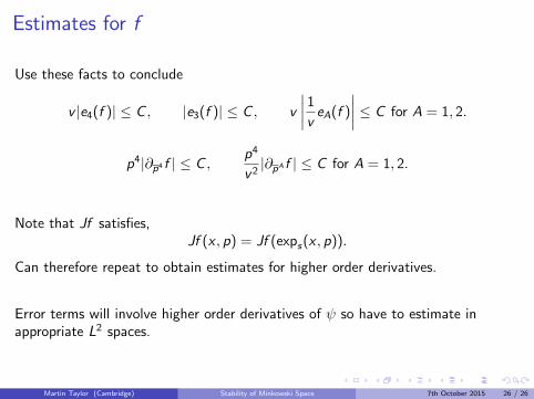
Estimates for f
Use these facts to conclude
v |e4(f )| ≤ C , |e3(f )| ≤ C , v
∣∣∣∣ 1v eA(f )
∣∣∣∣ ≤ C for A = 1, 2.
p4|∂p4 f | ≤ C ,p4
v2|∂pA f | ≤ C for A = 1, 2.
Note that Jf satisfies,Jf (x , p) = Jf (exps(x , p)).
Can therefore repeat to obtain estimates for higher order derivatives.
Error terms will involve higher order derivatives of ψ so have to estimate inappropriate L2 spaces.
Martin Taylor (Cambridge) Stability of Minkowski Space 7th October 2015 26 / 26