stability results in learning theory - statistics …rakhlin/papers/stability.pdf · 2008-12-24 ·...

October 14, 2005 14:37 WSPC/176-AA 00065

Analysis and Applications, Vol. 3, No. 4 (2005) 397–417c© World Scientific Publishing Company

STABILITY RESULTS IN LEARNING THEORY

ALEXANDER RAKHLIN

Center for Biological and Computational LearningMassachusetts Institute of Technology

45 Carleton St. E25-201, Cambridge, MA 02139, [email protected]

SAYAN MUKHERJEE

Institute of Genome Sciences and PolicyInstitute for Statistics and Decision SciencesDuke University, Durham, NC 27708, USA

[email protected]

TOMASO POGGIO

Center for Biological and Computational LearningMassachusetts Institute of Technology

Cambridge, MA 02139, [email protected]

Received 2 July 2005Revised 22 August 2005

The problem of proving generalization bounds for the performance of learning algorithmscan be formulated as a problem of bounding the bias and variance of estimators of theexpected error. We show how various stability assumptions can be employed for thispurpose. We provide a necessary and sufficient stability condition for bounding the biasand variance for the Empirical Risk Minimization algorithm, and various sufficient con-ditions for bounding bias and variance of estimators for general algorithms. We discusssettings in which it is possible to obtain exponential bounds, and we prove an extensionof the bounded-difference inequality for “almost always” stable algorithms.

Keywords: Stability; generalization; estimators; empirical risk minimization.

Mathematics Subject Classification 2000: 22E46, 53C35, 57S20

1. Introduction

One of the central problems of Statistical Learning Theory is to quantify the general-ization ability of learning algorithms within a probabilistic framework. The standardsetting for the problem is the following. Let F be a class of real-valued functions ona space X , mapping X into Y ⊂ R. Denote by µ an unknown probability measureon Z = X ×Y. An algorithm A is a mapping A : Zn �→ F , n ∈ Z

+. In plain words,a learning algorithm observes n input-output pairs and produces (learns) a function

397

October 14, 2005 14:37 WSPC/176-AA 00065

398 A. Rakhlin, S. Mukherjee & T. Poggio

which describes well the underlying input-output process. Throughout this article,we will focus on symmetric algorithms, i.e. A(z1, . . . , zn) = A(π(z1, . . . , zn)) for anypermutation π ∈ Sn, the symmetric group.

Let A(z1, . . . , zn; x) denote the evaluation of the function A(z1, . . . , zn) at apoint x. To measure the quality of A(z1, . . . , zn), a loss function � : F ×Z �→ [0, M ]is introduced, such that �(A(z1, . . . , zn); z) is a measure of how well A(z1, . . . , zn)predicts y at point x, where (x, y) = z ∈ Z. The function � is often taken to be thesquare loss.

If the algorithm A is clear from the context, we will write �(z1, . . . , zn; z) insteadof �(A(z1, . . . , zn); z). The functions �(f ; ·) are called the loss functions and the classL(F) = {�(f ; ·) : f ∈ F} is called the loss class.

The main quantity of interest is the expected error of the function A(z1, . . . , zn),

Iexp(z1, . . . , zn) := Ez∼µ[�(z1, . . . , zn; z)] =∫Z

�(z1, . . . , zn; z) dµ(z).

This quantity measures the accuracy of A(z1, . . . , zn) on the unseen data z drawnfrom µ. Unfortunately, the measure µ is unknown and this quantity cannot becomputed. The key assumption made in the Statistical Learning Theory is thatthe observed sample z1, . . . , zn is independent and identically distributed (i.i.d.)with the generating distribution µ. The problem thus is to estimate Iexp(z1, . . . , zn)based on the finite sample z1, . . . , zn.

Although the expected error is unknown, several important quantities can becomputed from the sample. The first one is the empirical error (or resubstitutionestimate),

Iemp(z1, . . . , zn) :=1n

n∑i=1

�(z1, . . . , zn; zi).

The second one is the leave-one-out error (or deleted estimate),a

Iloo(z1, . . . , zn) :=1n

n∑i=1

�(z1, . . . , zi−1, zi+1, . . . , zn; zi).

These quantities are employed to estimate the expected error, and the StatisticalLearning Theory is concerned with providing bounds on the deviations of theseestimates from the expected error. Denote these deviations

Ψn(z1, . . . , zn) := Iexp(z1, . . . , zn) − Iemp(z1, . . . , zn),

Φn(z1, . . . , zn) := Iexp(z1, . . . , zn) − Iloo(z1, . . . , zn).

If one can show that Ψn (or Φn) is “small”, then the empirical error (resp. leave-one-out error) is a good proxy for the expected error. In particular, we are interested in

aIt is understood that the first term in the sum is �(z2, . . . , zn; z1) and the last term is�(z1, . . . , zn−1; zn).

October 14, 2005 14:37 WSPC/176-AA 00065

Stability Results in Learning Theory 399

the rate of the convergence of Ψn and Φn to zero as n increases. Such statements,of course, have to be made in probability.

Let us first focus on the random variable Ψn(z1, . . . , zn). Recall that the CentralLimit Theorem (CLT) guarantees that the average of n i.i.d. random variables con-verges to their mean (under the assumption of finiteness of second moment). Unfor-tunately, the random variables �(z1, . . . , zn; z1), . . . , �(z1, . . . , zn; zn) are dependent,and the CLT is not applicable. In fact, the interdependence of these random vari-ables makes the resubstitution estimate positively biased, as the next example shows.

Example 1.1. Let X = [0, 1], Y = {0, 1}, µ(x) = U [0, 1], µ(y|x) = δy=1, �(y, y′) =|y−y′|, and A is defined as A(z1, . . . , zn; x) = 1 if x ∈ {x1, . . . , xn} and 0 otherwise.In other words, the algorithm observes n data points (x, 1), where x is distributeduniformly on [0, 1], and generates a hypothesis which fits exactly the observed data,but outputs 0 for unseen points x. The empirical error of A is 0, while the expectederror is 1, i.e. Ψn(z1, . . . , zn) = 1 for any z1, . . . , zn.

The algorithm in Example 1.1 is the Empirical Risk Minimization (ERM)algorithm

A(z1, . . . , zn) = argminf∈F

1n

n∑i=1

�(f ; zi).

In the above example, the function class F =⋃

n≥1{fx : x = (x1, . . . , xn) ∈ [0, 1]n}where fx(x) = 1 if x = xi for some 1 ≤ i ≤ n and fx(x) = 0 otherwise.

Though an exact minimizer of empirical risk might not exist, an almost-minimizer always exists. The results of this paper hold for almost-minimizers, but,for the sake of clarity, we consider exact minimization.

Minimizing the empirical error is a natural idea, as long as guarantees on small-ness of Ψn(z1, . . . , zn) can be made. Note that no such guarantee can be made inExample 1.1. Intuitively, this is due to the fact that the algorithm can fit any data,i.e. the space of functions L(F) is too large. Indeed, convergence of empirical errorsto the expected errors is completely characterized by the “size” of L(F). Such acharacterization disregards the algorithm A, and only focuses on the loss function� and the class F , from which the functions are chosen. The class L(F) is calleduniform Glivenko–Cantelli if for every ε > 0,

limn→∞ sup

µP

(sup

�∈L(F)

∣∣∣∣E� − 1n

n∑i=1

�(zi)∣∣∣∣ ≥ ε

)= 0,

where z1, . . . , zn are i.i.d. random variables distributed according to µ.Non-asymptotic results of the form

P

(sup

�∈L(F)

∣∣∣∣E� − 1n

n∑i=1

�(zi)∣∣∣∣ ≥ ε

)≤ δ(ε, n,L(F))

give uniform (over class L(F)) rates of convergence of empirical means to theexpected means. Since the guarantee is given for all functions in the class, the

October 14, 2005 14:37 WSPC/176-AA 00065


defect Ψn(z1, . . . , zn) is bounded by ε with probability 1− δ(ε, n,L(F)), no matterwhat the algorithm is.

Albeit interesting from the theoretical point of view, the uniform bounds are ingeneral loose, as they are “worst case” over all functions in the class. As an extremeexample, consider the algorithm that always ouputs the same function (the constantalgorithm)

A(z1, . . . , zn) = f0, ∀ (z1, . . . , zn) ∈ Zn.

The bound on Ψn(z1, . . . , zn) follows from the CLT and an analysis based upon thecomplexity of a class F does not make sense. Recent advances in the StatisticalLearning Theory shift the focus from uniform bounds to non-uniform bounds ofthe form

P(|Ψn(z1, . . . , zn)| > ε) < δ(ε, n,A), (1.1)

or

P(|Ψn(z1, . . . , zn)| > ε(δ, n,A, z1, . . . , zn)) < δ,

where in the last bound ε depends on the sample. In this article, we will focus on thebounds of type (1.1). The goal is to derive bounds on Ψn (or Φn) such thatlimn→∞ δ(ε, n,A) = 0 for any fixed ε > 0. If the rate of decrease of δ(ε, n,A) isnot important, we will write |Ψn| P→ 0 and |Φn| P→ 0.

Notice that Ψn and Φn are bounded random variables, as the loss function� ⊂ [0, M ]. By Markov’s inequality,

∀ ε ≥ 0, P(|Ψn| ≥ ε) ≤ E|Ψn|ε

and also,

∀ ε′ ≥ 0, E|Ψn| ≤ MP(|Ψn| ≥ ε′) + ε′.

Therefore, showing |Ψn| P→ 0 is equivalent to showing E|Ψn| → 0. The latter isequivalent to EΨ2

n → 0 since |Ψn| ≤ M . Further, notice that EΨ2n = var(Ψn) +

(EΨn)2. We will call EΨn the bias, var(Ψn) the variance, and EΨ2n the second

moment of Ψn. The same derivations and terminology hold for Φn.We have shown that studying conditions for convergence in probability of the

estimators to zero is equivalent to studying their mean and variance (or the secondmoment alone).

In this paper, we consider various stability conditions which allow one to boundbias and variance or the second moment, and thus imply convergence of Ψn andΦn to zero in probability. Though the reader should expect a number of definitionsof stability, the common flavor of these notions is the comparison of the “behavior”of the algorithm A on similar samples. We hope that the present work sheds lighton the important stability aspects of algorithms, suggesting principles for designingpredictive learning systems.

October 14, 2005 14:37 WSPC/176-AA 00065


We now sketch the organization of this paper. In Sec. 2, we motivate the use ofstability and give some historical background. In Sec. 3, we show how bias (Sec. 3.1)and variance (Sec. 3.2) can be bounded by various stability quantities. Sometimesit is mathematically more convenient to bound the second moment instead of biasand variance, and this is done in Sec. 4. In particular, Sec. 4.1 deals with the sec-ond moment EΦ2

n in the spirit of [4], while in Secs. 4.3 and 4.2, we bound EΨ2n in

the spirit of [10] and [2], respectively. The goal of Secs. 4.1 and 4.2 is to re-derivesome known results in a simple manner that allows one to compare the proofs sideby side. The results of these sections hold for general algorithms. Furthermore,for specific algorithms the results can be improved, i.e. simpler quantities mightgovern the convergence of the estimators to zero. To illustrate this, in Sec. 4.4 weprove that for the Empirical Risk Minimization algorithm, a bound on the biasEΨn implies a bound on the second moment EΨ2

n. We therefore provide a simplenecessary and sufficient condition for consistency of ERM. If rates of convergenceare of importance, rather than using Markov’s inequality, one can make use of moresophisticated concentration inequalities with a cost of requiring more stringent sta-bility conditions. In Sec. 5, we discuss the most rigid stability, Uniform Stability,and provide exponential bounds in the spirit of [2]. In Sec. 5.2, we consider less rigidnotions of stability and prove exponential inequalities based on powerful momentinequalities of [1]. Finally, Sec. 6 summarizes the paper and discusses further direc-tions and open questions.

2. Historical Remarks and Motivation

Devroye, Rogers and Wagner (see, e.g., [4]) were the first, to our knowledge, toobserve that sensitivity of the algorithms with regard to small changes in the sam-ple is related to the behavior of the leave-one-out estimate. The authors were able toobtain results for the k-Nearest-Neighbor algorithm, where VC theory fails becauseof large class of potential hypotheses. These results were further extended for k-localalgorithms and for potential learning rules. Kearns and Ron [6] later discovered aconnection between finite VC-dimension and stability. Bousquet and Elisseeff [2]showed that a large class of learning algorithms, based on Tikhonov Regulariza-tion, is stable in a very strong sense, which allowed the authors to obtain expo-nential bounds without much work. Kutin and Niyogi [8] introduced a number ofnotions of stability and showed implications between them. The authors emphasizedthe importance of “almost-everywhere” stability and proved valuable extensions ofMcDiarmid’s exponential inequality [7]. Mukherjee et al. [10] proved that a com-bination of three stability notions is sufficient to bound the difference between theempirical estimate and the expected error, while for Empirical Risk Minimizationthese notions are necessary and sufficient. The latter result showed an alternative toVC theory condition for consistency of Empirical Risk Minimization. In this paper,we prove, in a unified framework, some of the important results mentioned above,as well as show new ways of incorporating stability notions in the Learning Theory.

October 14, 2005 14:37 WSPC/176-AA 00065


We now give some intuition for using algorithmic stability. First, note thatwithout any assumptions on the algorithm, nothing can be said about the meanand the variance of Ψn. One can easily come up with settings when the mean isconverging to zero, but not the variance, or vice versa (e.g., Example 1.1), or bothquantities diverge from zero.

The assumptions of this paper that allow us to bound the mean and the vari-ance of Ψn and Φn are loosely termed as stability assumptions. Recall that if thealgorithm is a constant algorithm, Ψn is bounded by the Central Limit Theorem.Of course, this is an extreme and the most “stable” case. It turns out that the“constancy” assumption on the algorithm can be relaxed while still achieving tightbounds. A central notion here is that of Uniform Stability [2]:

Definition 2.1. Uniform Stability β∞(n) of an algorithm A is

β∞(n) := supz1,...,zn,z∈Z,x∈X

|A(z1, . . . , zn; x) −A(z, z2, . . . , zn; x)|.

Intuitively, if β∞(n) → 0, the algorithm resembles more and more the constantalgorithm when considered on similar samples (although it can produce distantfunctions on different samples). It can be shown that some well-known algorithmspossess Uniform Stability with a certain rate on β∞(n) (see [2] and Sec. 5.1).

In the following sections, we will show how the bias and variance (or secondmoment) can be upper-bounded or decomposed in terms of quantities over “similar”samples. The advantage of this approach is that it allows one to check “stability” fora specific algorithm and derive generalization bounds without much further work.For instance, it is easy to show that k-Nearest Neighbors algorithm is L1-stable anda generalization bound follows immediately (see Sec. 4.1).

3. Bounding Bias and Variance

3.1. Decomposing the bias

The bias of the resubstitution estimate and the deleted estimate can be written asquantities over similar samples:

EΨn = E

[1n

n∑i=1

[Ez�(z1, . . . , zn; z)− �(z1, . . . , zn; zi)

]]

= E[�(z1, . . . , zn; z) − �(z1, . . . , zn; z1)]

= E[�(z, z2, . . . , zn; z1) − �(z1, . . . , zn; z1)].

The first equality above follows because E�(z1, . . . , zn; zk) = E�(z1, . . . , zn; zm)for any k, m. The second equality holds by noticing that E�(z1, . . . , zn; z) =E�(z, z2, . . . , zn; z1) because the roles of z and z1 can be switched. We will employthis trick many times in the later proofs, and for convenience, we shall denote this“renaming” process by z ↔ z1.

Let us inspect the quantity E[�(z, z2, . . . , zn; z1) − �(z1, . . . , zn; z1)]. It is theaverage difference between the loss at a point z1 when it is not present in the

October 14, 2005 14:37 WSPC/176-AA 00065


learning sample (out-of-sample) and the loss at z1 when it is present in the n-tuple(in-sample). Hence, the bias EΨn will decrease if and only if the average behavioron in-sample and out-of-sample points is becoming more and more similar. This isa stability property and we will give a name to it:

Definition 3.1. Average Stability βbias(n) of an algorithm A is

βbias(n) := E[�(z, z2, . . . , zn; z1) − �(z1, . . . , zn; z1)].

We now turn to the deleted estimate. The bias EΦn can be written as

EΦn = E

[1n

n∑i=1

(Ez�(z1, . . . , zn; z) − �(z1, . . . , zi−1, zi+1, . . . , zn; zi))

]

= E[�(z1, . . . , zn; z) − �(z2, . . . , zn; z1)]

= E[Iexp(z1, . . . , zn) − Iexp(z2, . . . , zn)].

We will not give a name to this quantity, as it will not be used explicitly later. Onecan see that the bias of the deleted estimate should be small for reasonable algo-rithms. Unfortunately, the variance of the deleted estimate is large in general (see,e.g., [5, p. 415]). The opposite is believed to be true for the resubstitution estimate.We refer the reader to [5, Chaps. 23, 24 and 31] for more information. Surprisingly,we will show in Sec. 4.4 that for Empirical Risk Minimization algorithms, if oneshows that the bias of the resubstitution estimate decreases, one also obtains thatthe variance decreases.

3.2. Bounding the variance

Having shown a decomposition of the bias of Ψn and Φn in terms of stabilityconditions, we now show a simple way to bound the variance in terms of quantitiesover “similar” samples.

Theorem 3.2 (Efron–Stein). Let ξ : Zn �→ R be a measurable function ofn variables and define Γ = ξ(z1, . . . , zn) and Γ′

i = ξ(z1, . . . , z′i, . . . , zn), where

z1, . . . , zn, z′1, . . . , z′n are i.i.d. random variables. Then

var(Γ) ≤ 12

n∑i=1

E[(Γ − Γ′

i)2]. (3.1)

A “removal” version of the above is the following:

Theorem 3.3 (Efron–Stein). Let ξ : Zn �→ R be a measurable function of n

variables and ξ′ : Zn−1 �→ R of n − 1 variables. Define Γ = ξ(z1, . . . , zn) andΓi = ξ′(z1, . . . , zi−1, zi+1, . . . , zn), where z1, . . . , zn are i.i.d. random variables. Then

var(Γ) ≤n∑

i=1

E[(Γ − Γi)2

]. (3.2)

October 14, 2005 14:37 WSPC/176-AA 00065


The idea of the proofs of the above result is based on the fact that var(Γ) ≤E(Γ − c)2 for any constant c, and so

vari(Γ) = Ezi(Γ − EziΓ)2 ≤ Ezi(Γ − Γi)2.

Thus, we artificially introduce a quantity over a “similar” sample to upper-boundthe variance. If the increments Γ − Γi and Γ − Γ′

i are small, the variance is small.When applied to the function Ψn(z1, . . . , zn), this translates exactly into controllingthe behavior of A on similar samples:

var(Ψn) ≤ nE(Ψn(z1, . . . , zn) − Ψn(z2, . . . , zn))2

≤ 2nE(Iexp(z1, . . . , zn) − Iexp(z2, . . . , zn))2

+ 2nE(Iemp(z2, . . . , zn) − Iemp(z1, . . . , zn))2.

Here we used the fact that the algorithm is invariant under permutation of coordi-nates, and therefore all the terms in the sum of (3.2) are equal. This symmetry willbe exploited to a great extent in the later sections. Note that similar results can beobtained using the “replacement” version of Efron–Stein’s bound.

The meaning of the above bound is that if the mean square of the differencebetween expected errors of functions, learned from samples differing in one point,is decreasing faster than n−1, and if the same holds for the empirical errors, thenthe variance of the resubstitution estimate is decreasing. Let us give names to theabove quantities.

Definition 3.4. Empirical-Error (Removal) Stability of an algorithm A is

β2emp(n) := E|Iemp(z1, . . . , zn) − Iemp(z1, . . . , zi−1, zi+1, . . . , zn)|2.

Definition 3.5. Expected-Error (Removal) Stability of an algorithm A is

β2exp(n) := E|Iexp(z1, . . . , zn) − Iexp(z1, . . . , zi−1, zi+1, . . . , zn)|2.

With the above definitions, the following theorem follows:

Theorem 3.6.

var(Ψn) ≤ 2n(β2

exp(n) + β2emp(n)

).

The following example shows that the ERM algorithm is always Empirical-ErrorStable with βemp(n) ≤ M(n − 1)−1. We deduce that Ψn

P→ 0 for ERM wheneverβexp = o(n−1/2). As we will show in Sec. 4.4, the decay of the Average Stability,

βbias(n) = o(1), is both necessary and sufficient for ΨnP→ 0 for ERM.

October 14, 2005 14:37 WSPC/176-AA 00065


Example 3.7. For an Empirical Risk Minimization algorithm, βemp(n) ≤ Mn−1 :

Iemp(z2, . . . , zn) − Iemp(z1, . . . , zn)

≤ 1n − 1

n∑i=2

�(z2, . . . , zn; zi) − 1n − 1

n∑i=1

�(z1, . . . , zn; zi) +M

n − 1

≤ 1n − 1

n∑i=2

�(z2, . . . , zn; zi) − 1n − 1

n∑i=2

�(z1, . . . , zn; zi)

+M

n − 1− 1

n − 1�(z1, . . . , zn; z1) ≤ M

n − 1

and the other direction is proved similarly.

We will show in the following sections that a direct study of the second momentleads to better bounds. For the bound on the variance in Theorem 3.6 to decrease,βexp and βemp have to be o(n−1/2). With an additional assumption, we will be ableto remove the factor n by upper-bounding the second moment and by exploitingthe structure of the random variables Φn and Ψn.

4. Bounding the 2nd Moment

Instead of bounding the mean and variance of the estimators, we can bound thesecond moment. The reason for doing so is for mathematical convenience and isdue to the following straightforward bounds on the second moment:

EΨ2n = E[Ez�(z1, . . . , zn; z)]2 − E

[Ez�(z1, . . . , zn; z)

1n

n∑i=1

�(z1, . . . , zn; zi)

]

+ E

[1n

n∑i=1

�(z1, . . . , zn; zi)

]2

− E

[Ez�(z1, . . . , zn; z)

1n

n∑i=1

�(z1, . . . , zn; zi)

]

≤ E[Ez�(z1, . . . , zn; z)Ez′�(z1, . . . , zn; z′) − Ez�(z1, . . . , zn; z)�(z1, . . . , zn; z1)]

+ E[�(z1, . . . , zn; z1)�(z1, . . . , zn; z2) − Ez�(z1, . . . , zn; z)�(z1, . . . , zn; z1)]

+1n

E�(z1, . . . , zn; z1)2,

and the last term is bounded by M2

n . Similarly,

EΦ2n ≤ E[Ez�(z1, . . . , zn; z)Ez′�(z1, . . . , zn; z′) − Ez�(z1, . . . , zn; z)�(z2, . . . , zn; z1)]

+ E[�(z2, . . . , zn; z1)�(z1, z3, . . . , zn; z2) − Ez�(z1, . . . , zn; z)�(z2, . . . , zn; z1)]

+1n

E�(z2, . . . , zn; z1)2,

and the last term is bounded by M2

n .

October 14, 2005 14:37 WSPC/176-AA 00065


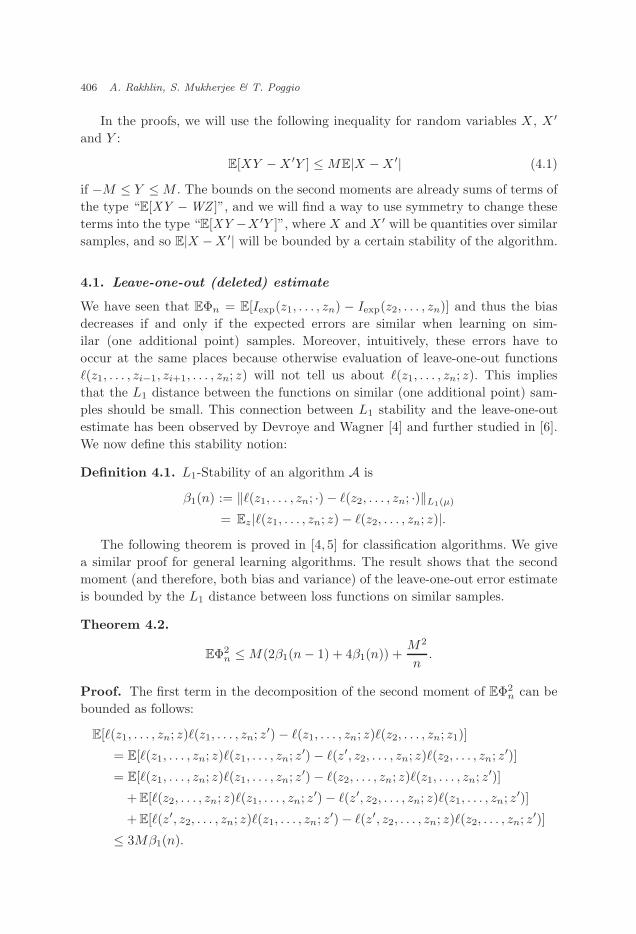
In the proofs, we will use the following inequality for random variables X , X ′

and Y :

E[XY − X ′Y ] ≤ ME|X − X ′| (4.1)

if −M ≤ Y ≤ M . The bounds on the second moments are already sums of terms ofthe type “E[XY − WZ ]”, and we will find a way to use symmetry to change theseterms into the type “E[XY −X ′Y ]”, where X and X ′ will be quantities over similarsamples, and so E|X −X ′| will be bounded by a certain stability of the algorithm.

4.1. Leave-one-out (deleted) estimate

We have seen that EΦn = E[Iexp(z1, . . . , zn) − Iexp(z2, . . . , zn)] and thus the biasdecreases if and only if the expected errors are similar when learning on sim-ilar (one additional point) samples. Moreover, intuitively, these errors have tooccur at the same places because otherwise evaluation of leave-one-out functions�(z1, . . . , zi−1, zi+1, . . . , zn; z) will not tell us about �(z1, . . . , zn; z). This impliesthat the L1 distance between the functions on similar (one additional point) sam-ples should be small. This connection between L1 stability and the leave-one-outestimate has been observed by Devroye and Wagner [4] and further studied in [6].We now define this stability notion:

Definition 4.1. L1-Stability of an algorithm A is

β1(n) := ‖�(z1, . . . , zn; ·) − �(z2, . . . , zn; ·)‖L1(µ)

= Ez |�(z1, . . . , zn; z) − �(z2, . . . , zn; z)|.The following theorem is proved in [4, 5] for classification algorithms. We give

a similar proof for general learning algorithms. The result shows that the secondmoment (and therefore, both bias and variance) of the leave-one-out error estimateis bounded by the L1 distance between loss functions on similar samples.

Theorem 4.2.

EΦ2n ≤ M(2β1(n − 1) + 4β1(n)) +

M2

n.

Proof. The first term in the decomposition of the second moment of EΦ2n can be

bounded as follows:

E[�(z1, . . . , zn; z)�(z1, . . . , zn; z′) − �(z1, . . . , zn; z)�(z2, . . . , zn; z1)]

= E[�(z1, . . . , zn; z)�(z1, . . . , zn; z′) − �(z′, z2, . . . , zn; z)�(z2, . . . , zn; z′)]

= E[�(z1, . . . , zn; z)�(z1, . . . , zn; z′) − �(z2, . . . , zn; z)�(z1, . . . , zn; z′)]

+ E[�(z2, . . . , zn; z)�(z1, . . . , zn; z′) − �(z′, z2, . . . , zn; z)�(z1, . . . , zn; z′)]

+ E[�(z′, z2, . . . , zn; z)�(z1, . . . , zn; z′) − �(z′, z2, . . . , zn; z)�(z2, . . . , zn; z′)]

≤ 3Mβ1(n).

October 14, 2005 14:37 WSPC/176-AA 00065


The first equality holds by renaming z′ ↔ z1. In doing this, we are using the factthat all the variables z1, . . . , zn, z, z′ are identically distributed and independent.To obtain the inequality above, note that each of the three terms is bounded (using(4.1)) by Mβ1(n) .

The second term in the decomposition is bounded similarly:

E[�(z2, . . . , zn; z1)�(z1, z3, . . . , zn; z2) − �(z1, . . . , zn; z)�(z2, . . . , zn; z1)]

= E[�(z′, z3, . . . , zn; z)�(z, z3, . . . , zn; z′) − �(z′, z2, . . . , zn; z)�(z2, . . . , zn; z′)]

= E[�(z′, z3, . . . , zn; z)�(z, z3, . . . , zn; z′) − �(z′, z2, . . . , zn; z)�(z, z3, . . . , zn; z′)]

+ E[�(z′, z2, . . . , zn; z)�(z, z3, . . . , zn; z′) − �(z′, z2, . . . , zn; z)�(z3, . . . , zn; z′)]

+ E[�(z′, z2, . . . , zn; z)�(z3, . . . , zn; z′) − �(z′, z2, . . . , zn; z)�(z2, . . . , zn; z′)]

≤ Mβ1(n) + 2Mβ1(n − 1).

The first equality follows by renaming z2 ↔ z′ as well as z1 ↔ z in the first term,and z1 ↔ z′ in the second term. Finally, we bound the last term by M2/n to obtainthe result.

4.2. Empirical error (resubstitution) estimate: replacement case

Recall that the bias of the resubstitution estimate is the Average Stability, EΨn =βbias. However, this is not enough to bound the second moment EΨ2

n for generalalgorithms. Nevertheless, βbias measures the average performance of in-sample andout-of-sample errors and this is inherently linked to the closeness of the resubsti-tution (in-sample) estimate and the expected error (out-of-sample performance). Itturns out that it is possible to derive bounds on EΨ2

n by using a stronger version ofthe Average Stability. The natural strengthening is requiring that not only the first,but also the second moment of �(z1, . . . , zn; zi)− �(z1, . . . , z

′i, . . . , zn; zi) is decaying

to 0. We follow [8] in calling this type of stability Cross-Validation (CV) Stability:

Definition 4.3. CV (Replacement) Stability of an algorithm A is

βcvr := E|�(z1, . . . , zn; z1) − �(z, z2, . . . , zn; z1)|,where the expectation is over a draw of n + 1 points.

The following theorem was proven in [2]. Here, we give a version of the proof.

Theorem 4.4.

EΨ2n ≤ 6Mβcvr(n) +

M2

n.

Proof. The first term in the decomposition of EΨ2n can be bounded as follows:

E[Ez�(z1, . . . , zn; z)Ez′�(z1, . . . , zn; z′) − Ez�(z1, . . . , zn; z)�(z1, . . . , zn; z2)]

= E[�(z1, z′, z3, . . . , zn; z)�(z1, z

′, z3, . . . , zn; z2) − �(z1, . . . , zn; z)�(z1, . . . , zn; z2)]

= E[�(z1, z′, z3, . . . , zn; z)�(z1, z

′, z3, . . . , zn; z2)

October 14, 2005 14:37 WSPC/176-AA 00065


− �(z1, z, z3, . . . , zn; z)�(z1, z′, z3, . . . , zn; z2)]

+ E[�(z1, z, z3, . . . , zn; z)�(z1, z′, z3, . . . , zn; z2)

− �(z1, . . . , zn; z)�(z1, z′, z3, . . . , zn; z2)]

+ E[�(z1, . . . , zn; z)�(z1, z′, z3, . . . , zn; z2) − �(z1, . . . , zn; z)�(z1, . . . , zn; z2)]

≤ 3Mβcvr(n).

The first equality follows from renaming z2 ↔ z′ in the first term. Each of the threeterms in the sum above is bounded by Mβcvr(n).

The second term in the decomposition of EΨ2n can be bounded as follows:

E [�(z1, . . . , zn; z1)�(z1, . . . , zn; z2) − Ez�(z1, . . . , zn; z)�(z1, . . . , zn; z1)]

= E [�(z, z2, . . . , zn; z)�(z, z2, . . . , zn; z2) − �(z1, . . . , zn; z)�(z1, . . . , zn; z2)]

= E [�(z, z2, . . . , zn; z)�(z, z2, . . . , zn; z2) − �(z1, . . . , zn; z)�(z, z2, . . . , zn; z2)]

+ E [�(z1, . . . , zn; z)�(z, z2, . . . , zn; z2)

− �(z1, . . . , zn; z)�(z1, z, z3, . . . , zn; z2)]

+ E [�(z1, . . . , zn; z)�(z1, z, z3, . . . , zn; z2) − �(z1, . . . , zn; z)�(z1, . . . , zn; z2)]

≤ 3Mβcvr(n).

The first equality follows by renaming z1 ↔ z in the first term. Again, each of thethree terms in the sum above can be bounded by Mβcvr(n).

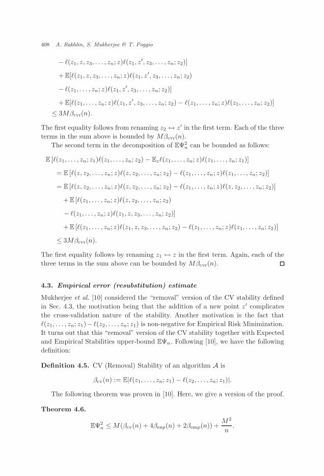
4.3. Empirical error (resubstitution) estimate

Mukherjee et al. [10] considered the “removal” version of the CV stability definedin Sec. 4.3, the motivation being that the addition of a new point z′ complicatesthe cross-validation nature of the stability. Another motivation is the fact that�(z1, . . . , zn; z1)− �(z2, . . . , zn; z1) is non-negative for Empirical Risk Minimization.It turns out that this “removal” version of the CV stability together with Expectedand Empirical Stabilities upper-bound EΨn. Following [10], we have the followingdefinition:

Definition 4.5. CV (Removal) Stability of an algorithm A is

βcv(n) := E|�(z1, . . . , zn; z1) − �(z2, . . . , zn; z1)|.The following theorem was proven in [10]. Here, we give a version of the proof.

Theorem 4.6.

EΨ2n ≤ M(βcv(n) + 4βexp(n) + 2βemp(n)) +

M2

n.

October 14, 2005 14:37 WSPC/176-AA 00065


Proof. The first term in the decomposition of the second moment of EΨ2n can be

bounded as follows:

E [�(z1, . . . , zn; z)�(z1, . . . , zn; z′) − �(z1, . . . , zn; z)�(z1, . . . , zn; z1)]

= E [�(z′, z2, . . . , zn; z)�(z′, z2, . . . , zn; z1) − �(z1, . . . , zn; z)�(z1, . . . , zn; z1)]

= E [�(z′, z2, . . . , zn; z)Ez1�(z′, z2, . . . , zn; z1)

− �(z′, z2, . . . , zn; z)Ez1�(z2, . . . , zn; z1)]

+ E [Ez�(z′, z2, . . . , zn; z)�(z2, . . . , zn; z1) − Ez�(z2, . . . , zn; z)�(z2, . . . , zn; z1)]

+ E [Ez�(z2, . . . , zn; z)�(z2, . . . , zn; z1) − Ez�(z1, . . . , zn; z)�(z2, . . . , zn; z1)]

+ E [�(z1, . . . , zn; z)�(z2, . . . , zn; z1) − �(z1, . . . , zn; z)�(z1, . . . , zn; z1)]

≤ M(3βexp(n) + βcv(n)).

The first equality follows by renaming z1 ↔ z in the first term. In the sum above,the first three terms are each bounded by Mβexp(n), while the last one is boundedby Mβcv(n). Since the Expected (and Empirical) Error Stability has been definedin Sec. 3.2 as expectation of a square, we used the fact that E|X | ≤ (EX2)1/2.

The second term in the decomposition of EΨ2n is bounded as follows:

E

24

0@ 1

n

nXi=1

�(z1, . . . , zn; zi)

1A

2

− Ez�(z1, . . . , zn; z)1

n

nXi=1

�(z1, . . . , zn; zi)

35

= E

"�(z1, . . . , zn; z1)

1

n

nXi=1

�(z1, . . . , zn; zi) − �(z1, . . . , zn; z)1

n

nXi=1

�(z1, . . . , zn; zi)

#

= E

"�(z1, . . . , zn; z1)

1

n

nXi=1

�(z1, . . . , zn; zi) − �(z2, . . . , zn; z1)1

n

nXi=1

�(z1, . . . , zn; zi)

#

+ E

"�(z2, . . . , zn; z1)

1

n

nXi=1

�(z1, . . . , zn; zi) − �(z2, . . . , zn; z)1

n − 1

nXi=2

�(z2, . . . , zn; zi)

#

+ E

"�(z2, . . . , zn; z)

1

n − 1

nXi=2

�(z2, . . . , zn; zi) − �(z2, . . . , zn; z)1

n

nXi=1

�(z1, . . . , zn; zi)

#

+ E

"Ez�(z2, . . . , zn; z)

1

n

nXi=1

�(z1, . . . , zn; zi) − Ez�(z1, . . . , zn; z)1

n

nXi=1

�(z1, . . . , zn; zi)

#

≤ M(βcv(n) + 2βemp(n) + βexp(n)).

The first equality follows by symmetry:

�(z1, . . . , zn; zk)1n

n∑i=1

�(z1, . . . , zn; zi) = �(z1, . . . , zn; zm)1n

n∑i=1

�(z1, . . . , zn; zi)

for all k, m. The first term in the sum above is bounded by Mβcv(n). The secondterm is bounded by Mβemp(n) (and z1 ↔ z). The third term is also bounded byMβemp(n), and the last term by Mβexp(n).

October 14, 2005 14:37 WSPC/176-AA 00065


4.4. Resubstitution estimate for the Empirical Risk Minimization

algorithm

It turns out that for the ERM algorithm, Ψn is “almost positive”. Intuitively, if oneminimizes the empirical error, then the expected error is likely to be larger thanthe empirical estimate. Since Ψn is “almost positive”, EΨn → 0 implies |Ψn| P→ 0.We now give a formal proof of this reasoning.

Recall, that an ERM algorithm searches in the function space F . Let

f∗ = arg minf∈F

Ez�(f ; z),

the minimizer of the expected error.b Consider the shifted loss class

L′(F) = {�′(f ; ·) = �(f ; ·) − �(f∗; ·)|f ∈ F}and note that Ez�

′(f ; z) ≥ 0 for any f ∈ F . Trivially, if �(z1, . . . , zn; ·) is an empiricalminimizer over the loss class L(F), then �′(f ; ·) = �(z1, . . . , zn; ·) − �(f∗; ·) is anempirical minimizer over the shifted loss class L′(F)

Ez�′(z1, . . . , zn; z) − 1

n

n∑i=1

�′(z1, . . . , zn; zi)

= Ez�(z1, . . . , zn; z) − 1n

n∑i=1

�(z1, . . . , zn; zi) −(

Ez�(f∗; z) − 1n

n∑i=1

�(f∗; zi)

).

Note that 1n

∑ni=1 �′(z1, . . . , zn; zi) ≤ 0 because L′(F) contains the zero function.

Therefore, the left-hand side is non-negative and the second term on the right-handside is small with high probability because f∗ is non-random. We have

P(Ψn(z1, . . . , zn) < −ε) ≤ P

(Ez�(f∗; z) − 1

n

n∑i=1

�(f∗; zi) < −ε

)≤ e−2nε2/M2

.

Therefore,

E|Ψn| ≤ EΨn + 2ε + 2Me−2nε2/M2.

If EΨn → 0, the right-hand side can be made arbitrarily small for large enough n,thus proving E|Ψn| → 0. Clearly, EΨn → 0 whenever E|Ψn| → 0. Hence, we havethe following theorem:

Theorem 4.7. For Empirical Risk Minimization, βbias(n) → 0 is equivalent to|Ψn| P→ 0.

Remark 4.8. With this approach, the rate of convergence of Iemp(z1, . . . , zn)to Iexp(z1, . . . , zn) is limited by the rate of convergence of 1

n

∑ni=1 �(f∗; zi) to

Ez�(f∗; z), which is O(n−1/2) without further assumptions.

bIf the minimizer does not exist, we consider ε-minimizer.

October 14, 2005 14:37 WSPC/176-AA 00065


For ERM, one can show that |Iemp(z1, . . . , zn) − Iemp(z2, . . . , zn)| ≤ Mn . Hence,

a “removal” version of Average Stability is closely related to Average Stability:

E (�(z1, . . . , zn; z1) − �(z2, . . . , zn; z1))

= E (Iemp(z1, . . . , zn) − Iexp(z2, . . . , zn))

= βbias(n − 1) + E (Iemp(z2, . . . , zn) − Iemp(z1, . . . , zn)) .

Thus, E (�(z1, . . . , zn; z1) − �(z2, . . . , zn; z1)) → 0 is also equivalent to |Ψn| P→ 0.Furthermore, one can show that

�(z1, . . . , zn; z1) − �(z2, . . . , zn; z1) ≥ 0

for ERM (see [10]), and so CV (Removal) Stability, defined in Sec. 4.3, is equal tothe above “removal” version of Average Stability. Hence, βcv(n) → 0 is equivalentto |Ψn| P→ 0.

Since Empirical Risk Minimization over a uniform Glivenko–Cantelli classimplies that |Ψn| P→ 0, it also implies that βbias(n) → 0 and βcv(n) → 0. Thus,ERM over a UGC class is stable in these regards. By using techniques from theEmpirical Process Theory, it can be shown (see [3]) that for ERM over a smallerfamily of classes, called Donsker classes, a much stronger stability in L1 norm (seeDefinition 4.1) holds: β1(n) → 0. Donsker classes are classes of functions satisfyingthe Central Limit Theorem, and for binary classes of function this is equivalent tofiniteness of the VC dimension.

5. Rates of Convergence

Previous sections focused on finding rather weak conditions for proving ΨnP→ 0 and

ΦnP→ 0 via Markov’s inequality. With stronger notions of stability, it is possible to

use more sophisticated inequalities, which is the focus of this section.

5.1. Uniform stability

Uniform Stability (see Definition 2.1), is a very strong notion, and we would notexpect, in general, that β∞(n) → 0. Surprisingly, for Tikhonov Regularizationalgorithms

A(z1, . . . , zn) = arg minf∈F

1n

n∑i=1

�(f ; zi) + λ‖f‖2K ,

it can be shown [2] that

β∞(n) ≤ L2κ2

2λn,

where F is a reproducing kernel Hilbert space (RKHS) with kernel K, K(x, x) ≤κ2 < ∞, ∀x ∈ X , and L is a Lipschitz constant relating norms between functionsf ∈ F to norms between loss functions � ∈ L(F).

October 14, 2005 14:37 WSPC/176-AA 00065


Clearly, β∞ dominates all stabilities discussed in the previous sections, and socan be used to bound the mean and variance of the estimators. For this strongstability, a more powerful concentration inequality can be used instead of Markov’sinequality. McDiarmid’s bounded difference inequality states that if a function ofmany random variables does not change much when one variable is changed, thenthe function is almost a constant. This is exactly what we need to bound Ψn or Φn.

Theorem 5.1 (McDiarmid, [9]). Let ξ : Zn �→ R be a measurable function,

Γ = ξ(z1, . . . , zn), Γ′i = ξ(z1, . . . , z

′i, . . . , zn), where z1, . . . , zn, z′1, . . . , z

′n are i.i.d.

random variables. If for all i,

supz1,...,zn,z′

1,...,z′n

|Γ − Γ′i| ≤ βn, (5.1)

then for any ε > 0,

P(|Γ − EΓ| ≥ ε) ≤ 2 exp(−2ε2

nβ2n

).

Bousquet and Elisseeff [2] applied this inequality to Γ = Ψn:

|Ψn(z1, . . . , zn) − Ψn(z1, . . . , z, . . . , zn)|≤ |Iemp(z1, . . . , zn) − Iemp(z, z2, . . . , zn)|

+ |Iexp(z1, . . . , zn) − Iexp(z, z2, . . . , zn)|

≤ 1n|�(z1, . . . , zn; z1) − �(z, z2, . . . , zn; z)|

+1n

n∑j=2

|�(z1, . . . , zn; zj) − �(z, z2, . . . , zn; zj)|

+ E′z|�(z1, . . . , zn; z′) − �(z, z2, . . . , zn; z′)|

≤ 2β∞(n) +M

n=: βn.

If β∞(n) = o(n−1/2), McDiarmid’s inequality shows that Ψn is exponentiallyconcentrated around EΨn, which is also small:

EΨn = βbias(n) ≤ β∞(n).

Therefore,

∀ ε > 0, P(Ψn ≥ β∞(n) + ε) ≤ 2 exp(− nε2

(2nβ∞(n) + M)2

).

Notice that for ERM, |Iemp(z1, . . . , zn) − Iemp(z, z2, . . . , zn)| ≤ Mn and so it is

enough to require βbias → 0 and |Iexp(z1, . . . , zn) − Iexp(z, z2, . . . , zn)| = o(n−1/2)to get exponential bounds. The last requirement is strong, as it requires expectederrors on similar samples to be close for every sample. The next section deals with“almost-everywhere” stabilities (see [8]), i.e. when a stability quantity is small formost samples.

October 14, 2005 14:37 WSPC/176-AA 00065


5.2. Extending McDiarmid’s inequality

As one extreme, if we know that β∞(n) = o(n−1/2), we can use exponentialMcDiarmid’s inequality. As the other extreme, if we only have information aboutaverages βemp and βexp, we are forced to use the second moment and Chebyshev’sor Markov’s inequality. What happens in between these extremes? What if we knowmore about the random variables Iemp(z1, . . . , zn)− Iemp(z, z2, . . . , zn)? One exam-ple is the case when we know that these random variables are almost always small.Unfortunately, assumptions of McDiarmid’s inequality are no longer satisfied, soother ways of deriving exponential bounds are needed. This section elaborates onthis situation.

Assume that for a given βn, a measurable function ξ : Zn �→ [−M, M ] satisfiesthe bounded difference condition (5.1) on a subset G ⊆ Zn of measure 1−δn, while

∀ (z1, . . . , zn) ∈ G, ∃ z′i ∈ Zs.t. βn < |ξ(z1, . . . , zn)−ξ(z1, . . . , z

′i, . . . , zn)| ≤ 2M,

where G is the complement of the subset G. Again, denote Γ = ξ(z1, . . . , zn),Γ′

i = ξ(z1, . . . , z′i, . . . , zn). A simple application of Efron–Stein inequality shows that

var(Γ) ≤ 12nE (ξ(z1, . . . , zn) − ξ(z, z2, . . . , zn))2

≤ 12nE

[I(z1,...,zn)∈G (ξ(z1, . . . , zn) − ξ(z, z2, . . . , zn))2

]+

12nE

[I(z1,...,zn)∈G (ξ(z1, . . . , zn) − ξ(z, z2, . . . , zn))2

]≤ 1

2n(β2

n + 4M2δn). (5.2)

This leads to a polynomial bound on P(|Γ − EΓ| ≥ ε). Kutin and Niyogi [7, 8]proved an inequality which is exponential when δn decays exponentially with n,thus extending McDiarmid’s inequality to incorporate a small possibility of a largejump of ξ. A more general version of their bound is the following:

Theorem 5.2 (Kutin and Niyogi [8]). Assume ξ : Zn �→ [−M, M ] satisfiesthe bounded difference condition (5.1) on a set of measure 1 − δn and denote Γ =ξ(z1, . . . , zn). Then, for any ε > 0,

P(|Γ − EΓ| ≥ ε) ≤ 2 exp( −ε2

8nβ2n

)+

2Mnδn

βn. (5.3)

Note that the bound tightens only if βn = o(n−1/2) and δn/βn = o(n−1).Furthermore, the bound is exponential only if δn decays exponentially.c

While the variance bound in (5.2) is written in terms of the second moment, wecan use powerful moment inequalities, recently developed by Boucheron et al. [1],

cBy exponential rate, we mean decay o(exp(−nr)) for a fixed r > 0.

October 14, 2005 14:37 WSPC/176-AA 00065


to bound the qth moment of Γ. Moreover, q can be optimized to get the tightestbounds.d

Define random variables V+ and V− as

V+ = E

[n∑

i=1

(Γ − Γ′i)

2IΓ≥Γ′i|z1, . . . , zn

], V− = E

[n∑

i=1

(Γ − Γ′i)

2IΓ<Γ′i|z1, . . . , zn

].

Theorem 5.3 (Boucheron et al. [1]). For ξ : Zn �→ R, Γ = ξ(z1, . . . , zn), andany q ≥ 2,

‖(Γ − EΓ)+‖q ≤√

2κq‖√

V+‖q and ‖(Γ − EΓ)−‖q ≤√

2κq‖√

V+‖q,

where x+ = max(0, x) and κ ≈ 1.271 is a constant.

This result leads directly to the following theorem:

Theorem 5.4. Assume ξ : Zn �→ R satisfies the bounded difference condition (5.1)on a set of measure 1 − δn, and denote Γ = ξ(z1, . . . , zn). Then for any q ≥ 2and ε > 0,

P(Γ − EΓ > ε) ≤ (nq)q/2((2κ)q/2βqn + (2M)qδn)

εq,

where κ ≈ 1.271.

Proof.

EVq/2+ = E

{IGV

q/2+ + IGV

q/2+

} ≤ (nβ2n)q/2 + (nq(2M)2)q/2δn.

By Theorem 5.3,

E(Γ − EΓ)q+ ≤ (2κq)q/2

EVq/2+ ≤ (nβ2

nq2κ)q/2 + (n(2M)2)q/2δn.

Hence,

P(Γ − EΓ > ε) ≤ E(Γ − EΓ)q+

εq≤ (nq)q/2((2κ)q/2βq

n + (2M)qδn)εq

.

Note that the bound of Theorem 5.4 holds for any q ≥ 2. To clarify theasymptotic behavior of the bound, assume βn = n−γ for some γ > 1/2, and letq = ε2β−2

n n−2γ+η = ε2nη for some η to be chosen later, 2γ − 1 > η > 0. Assumeδn = exp(n−θ) for some θ > 0. The bound of Theorem 5.4 becomes

P(Γ − EΓ > ε) ≤ (nq)q/2((2κ)q/2βqn + (2M)qδn)

εq

≤(

2κnqβ2n

ε2

)q/2

+ δn

(4M2nq

ε2

)q/2

≤ (2κn1+η−2γ) ε2

2 nη

+(4M2n1+η

) ε22 nη

exp(−nθ)

dThanks to Gabor Lugosi for suggesting this method.

October 14, 2005 14:37 WSPC/176-AA 00065


≤ exp(

(1 + (1 + η − 2γ) log n)nη ε2

2

)

+ exp(

(2 log(2M) + (1 + η) log n)nη ε2

2− nθ

). (5.4)

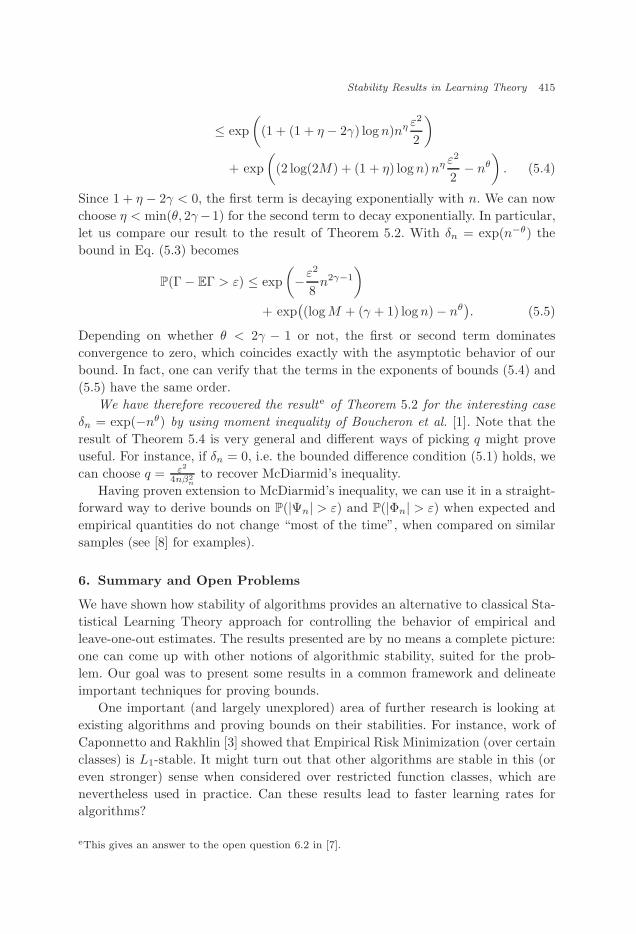
Since 1 + η − 2γ < 0, the first term is decaying exponentially with n. We can nowchoose η < min(θ, 2γ−1) for the second term to decay exponentially. In particular,let us compare our result to the result of Theorem 5.2. With δn = exp(n−θ) thebound in Eq. (5.3) becomes

P(Γ − EΓ > ε) ≤ exp(−ε2

8n2γ−1

)+ exp

((log M + (γ + 1) log n) − nθ

). (5.5)

Depending on whether θ < 2γ − 1 or not, the first or second term dominatesconvergence to zero, which coincides exactly with the asymptotic behavior of ourbound. In fact, one can verify that the terms in the exponents of bounds (5.4) and(5.5) have the same order.

We have therefore recovered the resulte of Theorem 5.2 for the interesting caseδn = exp(−nθ) by using moment inequality of Boucheron et al. [1]. Note that theresult of Theorem 5.4 is very general and different ways of picking q might proveuseful. For instance, if δn = 0, i.e. the bounded difference condition (5.1) holds, wecan choose q = ε2

4nβ2n

to recover McDiarmid’s inequality.Having proven extension to McDiarmid’s inequality, we can use it in a straight-

forward way to derive bounds on P(|Ψn| > ε) and P(|Φn| > ε) when expected andempirical quantities do not change “most of the time”, when compared on similarsamples (see [8] for examples).

6. Summary and Open Problems

We have shown how stability of algorithms provides an alternative to classical Sta-tistical Learning Theory approach for controlling the behavior of empirical andleave-one-out estimates. The results presented are by no means a complete picture:one can come up with other notions of algorithmic stability, suited for the prob-lem. Our goal was to present some results in a common framework and delineateimportant techniques for proving bounds.

One important (and largely unexplored) area of further research is looking atexisting algorithms and proving bounds on their stabilities. For instance, work ofCaponnetto and Rakhlin [3] showed that Empirical Risk Minimization (over certainclasses) is L1-stable. It might turn out that other algorithms are stable in this (oreven stronger) sense when considered over restricted function classes, which arenevertheless used in practice. Can these results lead to faster learning rates foralgorithms?

eThis gives an answer to the open question 6.2 in [7].

October 14, 2005 14:37 WSPC/176-AA 00065


Adding a regularization term for ERM leads to an extremely stable TikhonovRegularization algorithm. How can regularization be used to stabilize other algo-rithms, and how does this affect the bias-variance trade-off of fitting the data versushaving a simple solution?

Though the results presented in this paper are theoretical, there is a potentialfor estimating stability in practice. Can a useful quantity be computed by runningthe algorithm many times to determine its stability? Can this quantity serve as ameasure of the performace of the algorithm?

Acknowledgments

This report describes research done at the Center for Biological and Compu-tational Learning, which is in the McGovern Institute for Brain Research atMIT, as well as in the Department of Brain and Cognitive Sciences, and whichis affiliated with the Computer Sciences and Artificial Intelligence Laboratory(CSAIL). This research was sponsored by grants from: Office of Naval Research(DARPA) Contract No. MDA972-04-1-0037, Office of Naval Research (DARPA)Contract No. N00014-02-1-0915, National Science Foundation (ITR/IM) Con-tract No. IIS-0085836, National Science Foundation (ITR/SYS) Contract No. IIS-0112991, National Science Foundation (ITR) Contract No. IIS-0209289, NationalScience Foundation-NIH (CRCNS) Contract No. EIA-0218693, National ScienceFoundation-NIH (CRCNS) Contract No. EIA-0218506, and National Institutesof Health (Conte) Contract No. 1 P20 MH66239-01A1. Additional support wasprovided by: Central Research Institute of Electric Power Industry, Center fore-Business (MIT), Daimler-Chrysler AG, Compaq/Digital Equipment Corporation,Eastman Kodak Company, Honda R&D Co. Ltd., ITRI, Komatsu Ltd., EugeneMcDermott Foundation, Merrill-Lynch, Mitsubishi Corporation, NEC Fund,Nippon Telegraph & Telephone, Oxygen, Siemens Corporate Research Inc., SonyMOU, Sumitomo Metal Industries, Toyota Motor Corporation, and WatchVisionCo. Ltd.

References

[1] S. Boucheron, O. Bousquet, G. Lugosi and P. Massart, Moment inequalities for func-tions of independent random variables, Ann. Probab. 33(2) (2005) 514–560.

[2] O. Bousquet and A. Elisseeff, Stability and generalization, J. Mach. Learn. Res.2 (2002) 499–526.

[3] A. Caponnetto and A. Rakhlin, Some properties of Empirical Risk Minimization overDonsker classes, AI Memo 2005-018, Massachusetts Institute of Technology (May2005).

[4] L. P. Devroye and T. J. Wagner, Distribution-free performance bounds for potentialfunction rules, IEEE Trans. Inform. Theory 25(5) (1979) 601–604.

[5] L. Devroye, L. Gyorfi and G. Lugosi, A Probabilistic Theory of Pattern Recognition,Applications of Mathematics, No. 31 (Springer, New York, 1996).

October 14, 2005 14:37 WSPC/176-AA 00065


[6] M. J. Kearns and D. Ron, Algorithmic stability and sanity-check bounds for leave-one-out cross-validation, in COLT (1997), pp. 152–162.

[7] S. Kutin, Extensions to McDiarmid’s inequality when differences are bounded withhigh probability, Technical report TR-2002-04, University of Chicago (2002).

[8] S. Kutin and P. Niyogi, Almost-everywhere algorithmic stability and generalizationerror, Technical report TR-2003-03, University of Chicago (2002).

[9] C. McDiarmid, On the method of bounded differences, In Surveys in Combinatorics1989 (1989), pp. 148–188.

[10] S. Mukherjee, P. Niyogi, T. Poggio and R. Rifkin, Statistical learning: Stability isnecessary and sufficient for consistency of empirical risk minimization, CBCL Paper2002-023, Massachusetts Institute of Technology (December 2002) (January 2004revision).

stability results in learning theory - statistics …rakhlin/papers/stability.pdf · 2008-12-24 ·...

Documents