staff paper - ageconsearch.umn.eduageconsearch.umn.edu/bitstream/11757/1/sp01-53.pdfstaff paper...

Staff Paper

Deterministic Nonparametric Market PowerTests: An Empirical Investigation

Corinna M. [email protected]

Kellie Curry [email protected]

Staff Paper 2001-53 November 2001

Department of Agricultural EconomicsMICHIGAN STATE UNIVERSITY

East Lansing, Michigan 48824MSU is an Affirmative Action/Equal Opportunity Institution

DETERMINISTIC NONPARAMETRIC MARKET POWER TESTS:AN EMPIRICAL INVESTIGATION

Corinna M. Noelke*Manager, International Financial Reporting and Coordination

Random House, Inc.1540 Broadway

New York, NY 10036(212) 782-9217

(212) 782-8226 [email protected]

Kellie Curry Raper*(Corresponding Author)

Department of Agricultural Economics211C Agriculture Hall

Michigan State UniversityEast Lansing, MI 48824-1039

(517) 353-7226(517) 432-1800 FAX

[email protected]

26 pages

Abstract: A review of recent literature reflects the development of several deterministic nonparametricmarket power tests. We use Monte Carlo experiments to evaluate the veracity of four monopolistic and fourmonopsonistic market power tests that use the deterministic nonparametric approach. The experiments areimplemented using data from ten known market structures. When results are compared to Raper, Love, andShumway’s (1999) findings concerning parametric market power tests in the Bresnahan-Lau tradition, wefind that the parametric tests perform well while only two of the nonparametric tests appear able to identifymarket power.

Keywords: market power, Monte Carlo, nonparametric, monopoly, monopsony.JEL Classification: L1.______________________*Corinna M. Noelke is Manager, International Financial Reporting and Coordination, Random House,Inc., New York, New York and Kellie Curry Raper is Assistant Professor, Department of AgriculturalEconomics, Michigan State University. This research was supported in part by the Michigan AgriculturalExperiment Station, East Lansing, Michigan and in part by a USDA Cooperative State Research,Education, and Extension Service (CSREES) Special Grant to the Food Marketing Policy Center,University of Connecticut, and by subcontract at the University of Massachusetts, Amherst.

Copyright: 2001 by Corinna M. Noelke and Kellie Curry Raper. All rights reserved. Readers may make verbatim copiesof this document for non-commercial purposes by any means, provided that this copyright notice appears on all such copies.

DETERMINISTIC NONPARAMETRIC MARKET POWER TESTS:AN EMPIRICAL INVESTIGATION

Abstract: A review of recent literature reflects the development of several deterministic nonparametricmarket power tests. We use Monte Carlo experiments to evaluate the veracity of four monopolistic and fourmonopsonistic market power tests that use the deterministic nonparametric approach. The experiments areimplemented using data from ten known market structures. When results are compared to Raper, Love, andShumway’s (1999) findings concerning parametric market power tests in the Bresnahan-Lau tradition, wefind that the parametric tests perform well while only two of the nonparametric tests appear able to identifymarket power.

Keywords: market power, Monte Carlo, nonparametric, monopoly, monopsony.

JEL Classification: L1.

1We do not follow the Chicago School which asserts that markups are due to efficiency.This efficiency lowers costs which translates into lower prices and thus benefits consumers. Thebenefits are assumed to be greater than under the situation where less efficient but competitivefirms which do not charge a markup, have higher costs so that prices are in the end higher thanfrom a more efficient firm.

1

1. Introduction

In economic theory, monopolymarket power is the ability to set price greater than marginal cost, that

is, above the competitive level where prices are presumed equal to marginal cost.1 If market power is

exerted, deadweight welfare loss occurs. This denotes, in the case of monopoly power exertion, that

consumer surplus decreases, producers receive a surplus (profit), and some of the former consumer surplus

becomes a loss to society. Knowledge of the degree of market power exertion is used to guide decisions

regarding merger policy or antitrust enforcement in such markets. Thus, it is important to be able to detect

monopolistic or monopsonistic behavior by a firm or industry to assess whether the market structure should

be changed through, for example, government intervention. An example is the United States Department of

Agriculture's (USDA) Grain Inspection, Packers and Stockyards Administration's (GIPSA) recent

investigation into monopsony power exertion by meat packers in procuring live cattle. Significant evidence

of imperfectly competitive behavior by packers could lead to new regulations regarding price reporting, the

cattle bidding process, or ultimately to a breakup of the packers by the Justice Department.

Three major approaches to measurement of market power exertion have developed within New

Empirical IndustrialOrganization (NEIO): parametric, nonstructural, and nonparametric market power tests.

In this paper, we will focus on deterministic nonparametric market power tests and their performance

compared to parametric market power tests. Both, parametric and deterministic nonparametric market power

tests develop from profit maximization assumptions and result in direct measures of market power exertion.

The parametric approach econometrically estimates market power by parameterizing the monopoly

2

(monopsony) markup (markdown) term (Appelbaum 1979; Bresnahan 1982; Lau 1982). It relies on a

calculus approach which assumes that the entire demand and supply function is available for analysis.

Parametric tests yield testable hypotheses regarding market power exertion. However, these hypotheses

depend on the functional form chosen for the underlying model. Additionally, econometric identification of

the market power parameter restricts functional form choice somewhat.

The deterministic nonparametric approach to market power measurement is relatively new and

developed in response to criticisms of the parametric approach (Ashenfelter and Sullivan 1987; Driscoll,

Kambhampaty and Purcell 1997; Lambert 1994; Love and Shumway 1994; Ussif and Lambert 1998).

Deterministic nonparametric tests are an exhaustive search for violations of the given hypothesis using an

algebraic approach assuming onlya finite number of observations on firm behavior. In contrast to parametric

tests, deterministic nonparametric tests do not require ad hoc specifications offunctionalformfor production,

cost, profit, supply, or demand functions, so the problem of testing joint hypotheses is avoided (Varian 1984;

Varian 1985; Varian 1990). Additionally, less data is required than for parametric tests because opposing

supply or demand curves are not needed and they can handle disaggregated inputs and multiple output

technologies. However, deterministic nonparametric tests are not imbedded in a stochastic framework, that

is, “the data are assumed to be observed without error, so that the tests are ‘all or nothing’: either the data

satisfy the optimization hypothesis or they don’t” (Varian 1985, pg. 445). This can result in the possible

rejection of hypotheses that are only violated once because the magnitude of violations is not considered.

Various authors argue the merits of each type of market power test (Ashenfelter and Sullivan 1987;

Hyde and Perloff 1994; Hyde and Perloff 1995), but to date no comprehensive comparison of the

performance of deterministic nonparametric and parametric tests has been conducted. For comparison of

performance, it is necessary to apply the tests to data where the degree of market power exertion is known.

3

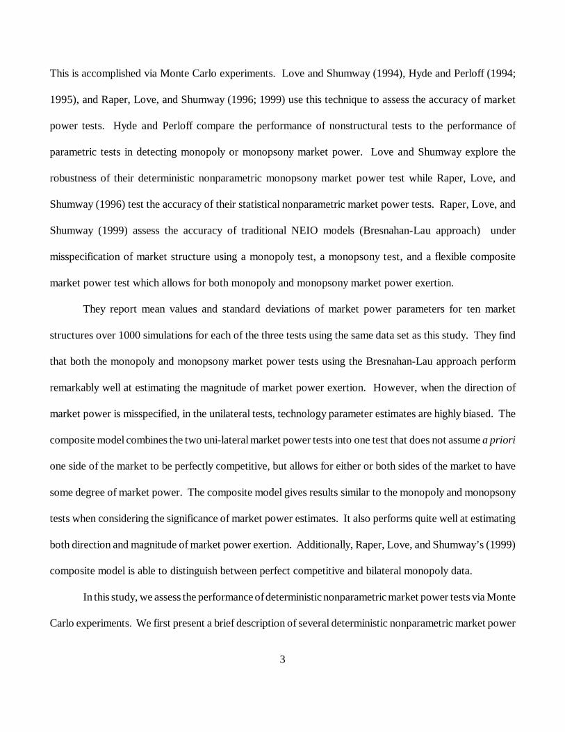
This is accomplished via Monte Carlo experiments. Love and Shumway (1994), Hyde and Perloff (1994;

1995), and Raper, Love, and Shumway (1996; 1999) use this technique to assess the accuracy of market

power tests. Hyde and Perloff compare the performance of nonstructural tests to the performance of

parametric tests in detecting monopoly or monopsony market power. Love and Shumway explore the

robustness of their deterministic nonparametric monopsony market power test while Raper, Love, and

Shumway (1996) test the accuracy of their statistical nonparametric market power tests. Raper, Love, and

Shumway (1999) assess the accuracy of traditional NEIO models (Bresnahan-Lau approach) under

misspecification of market structure using a monopoly test, a monopsony test, and a flexible composite

market power test which allows for both monopoly and monopsony market power exertion.

They report mean values and standard deviations of market power parameters for ten market

structures over 1000 simulations for each of the three tests using the same data set as this study. They find

that both the monopoly and monopsony market power tests using the Bresnahan-Lau approach perform

remarkably well at estimating the magnitude of market power exertion. However, when the direction of

market power is misspecified, in the unilateral tests, technology parameter estimates are highly biased. The

composite model combines the two uni-lateral market power tests into one test that does not assume a priori

one side of the market to be perfectly competitive, but allows for either or both sides of the market to have

some degree of market power. The composite model gives results similar to the monopoly and monopsony

tests when considering the significance of market power estimates. It also performs quite well at estimating

both direction and magnitude of market power exertion. Additionally, Raper, Love, and Shumway’s (1999)

composite model is able to distinguish between perfect competitive and bilateral monopoly data.

In this study, we assess the performance ofdeterministic nonparametric market power tests via Monte

Carlo experiments. We first present a brief description of several deterministic nonparametric market power

4

tests from the literature. Then, we implement these tests using Raper, Love, and Shumway’s (1999)

simulated data from 10 different market structures, including perfect competition, monopoly, monopsony,

Cournot and Stackelberg duopoly and duopsony, and three forms of cooperative bilateral monopoly. We

compare the performance of these deterministic nonparametric tests to each other and to that of Bresnahan-

Lau type parametric market power tests as reported in Raper, Love, and Shumway (1999). Thus, in this

study, we hope to add to the knowledge base regarding which tests should be used in the future to determine

whether a firm and/or industry exerts market power.

2. Deterministic Nonparametric Tests

Deterministic nonparametric tests, which employ a revealed preference approach, were introduced

by Afriat (1972), Hanoch and Rothschild (1972), Diewert and Parkan (1983), and Varian (1984) in the

production economics literature. Varian (1984) proposed the Monopolistic Axiom of Profit Maximization

(MAPM) which gives the conditions under which observed behavior can be rationalized as monopolistic

behavior. Ashenfelter and Sullivan (Ashenfelter and Sullivan 1987) developed the first deterministic

nonparametric monopolymarket power test based on the Weak Axiom of Profit Maximization (WAPM) that

directly measures the importance of the monopoly markup term in profit maximization.. Others followed in

developing market power tests with foundations in this literature (Driscoll, Kambhampaty and Purcell 1997;

Lambert 1994; Love and Shumway 1994; Ussif and Lambert 1998). The general approach measures the

importance of the monopoly markup or monopsony markdown term in profit maximization. In the case of

monopsony power, market power translates to an input price less than the value of marginal product. In the

case of monopoly power, market power translates to an output price higher than the marginal cost of

production. For consistency with competitive behavior, WAPM states that the observed input and output

5

∆π i ' p∆yi % y i∆p & jn

m'1

w m∆zmi # 0 ,(3)

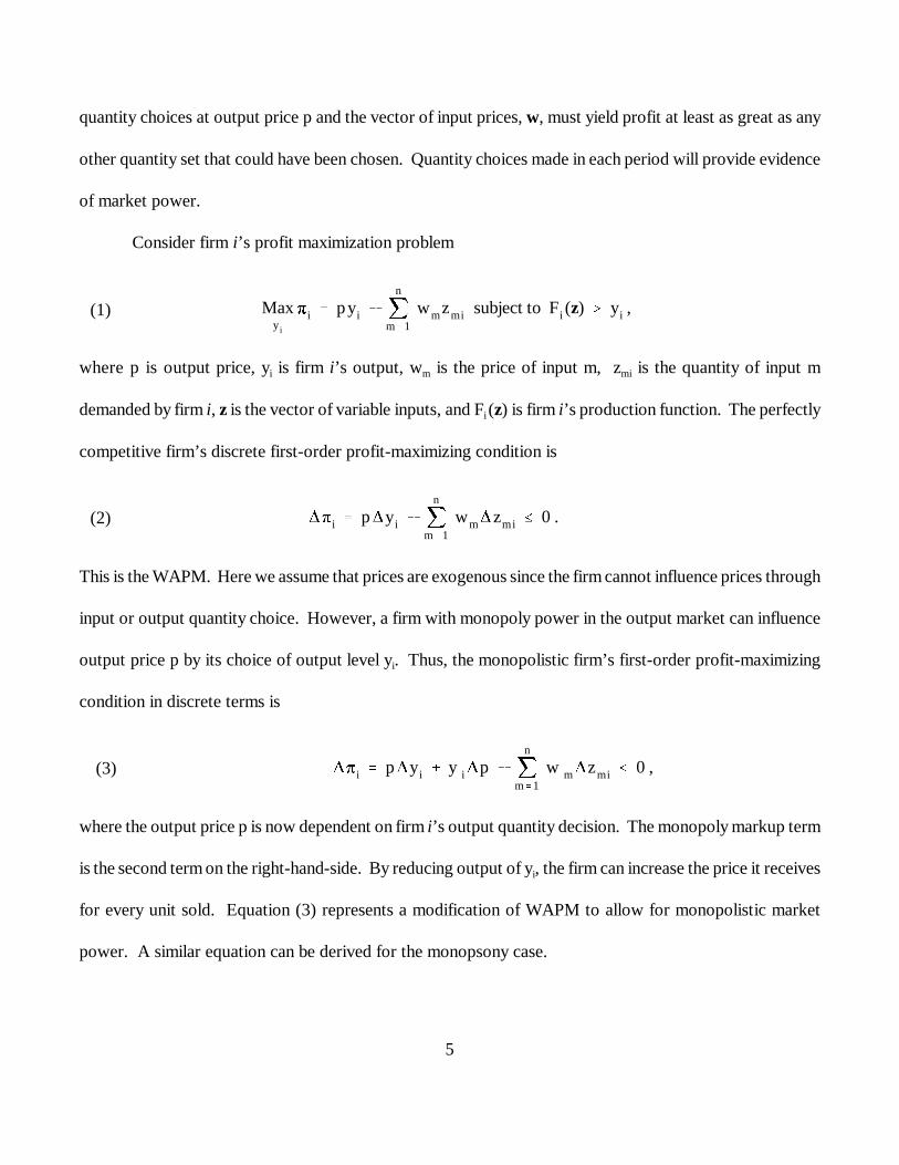
quantity choices at output price p and the vector of input prices, w, must yield profit at least as great as any

other quantity set that could have been chosen. Quantity choices made in each period will provide evidence

of market power.

Consider firm i’s profit maximization problem

Maxyi

π i ' pyi & jn

m'1

wmzmi subject to Fi (z) $ yi ,(1)

where p is output price, yi is firm i’s output, wm is the price of input m, zmi is the quantity of input m

demanded by firm i, z is the vector of variable inputs, and Fi(z) is firm i’s production function. The perfectly

competitive firm’s discrete first-order profit-maximizing condition is

∆π i ' p∆yi & jn

m'1

wm∆zmi # 0 .(2)

This is the WAPM. Here we assume that prices are exogenous since the firm cannot influence prices through

input or output quantity choice. However, a firm with monopoly power in the output market can influence

output price p by its choice of output level yi. Thus, the monopolistic firm’s first-order profit-maximizing

condition in discrete terms is

where the output price p is now dependent on firm i’s output quantity decision. The monopoly markup term

is the second term on the right-hand-side. By reducing output of yi, the firm can increase the price it receives

for every unit sold. Equation (3) represents a modification of WAPM to allow for monopolistic market

power. A similar equation can be derived for the monopsony case.

6

∆π i ' p∆yi & jn&1

m'1

wm∆zmi & wn∆zni & zni∆w n # 0 ,(4)

where the monopsony markdown term is the fourth term on the right hand side. By reducing the quantity

bought of the monopsonistically exerted input zni bought, the firm can decrease the price, wn, it has to pay

for this input.

2.1 Ashenfelter and Sullivan Method

Ashenfelter and Sullivan (1987) were the first to test for monopoly market power exertion using the

deterministic nonparametric approach. They construct a deterministic nonparametric test of the monopoly

model based on revealed preference arguments and extend the test to assess the validity of some less extreme

oligopoly models. They make two assumptions that simplify the empirical implementation: (1) the

assumption of increasing costs and (2) the maintained hypothesis that variations in the excise tax are

equivalent to changes in marginal cost. This allows Ashenfelter and Sullivan to drop input costs from the

equation since their exclusion will not affect the equation’s integrity. The monopoly markup term is

parameterized and its parameter, , lies between zero for perfect competition and one for monopoly whileβmp

values in between correspond to oligopoly situations. The parameter is thus an equivalent to the Lernerβmp

index (1934) of monopoly market power, , which exhibits these properties under theL '

P & MCP

assumption that a monopolist does not operate in the inelastic portion of the demand curve. Ashenfelter and

Sullivan adjust also for structural shifts (shifts in the demand or cost functions) by comparing only

observations no more than two years apart, but do not incorporate the possibility of technical change. The

original industry-level monopoly market power test is

7

βmp #& (p t

& e s) (y t& y s)

(p t& p s) y s

œ t … s where * t & s* # 2 ,(5)

where t and s represent time periods, with t = 1, 2, ..., T and es is the excise tax. Applying this model to the

U.S. cigarette industry from1955 to 1982 by state, they find little evidence for the monopolyhypothesis (true

only 37% of the time). Additionally, they calculate a Cournot numbers equivalent (CNE) which is greater

or equal to the inverse of . More than 75% of the data support the hypothesis that the U.S. cigaretteβmp

industry behaves equivalent to having five or six Cournot-type firms in the market. More than 86.5% of the

data support the hypothesis that the industry works as if nine Cournot-firms compete in the same market.

To generalize this test to industries that do not exhibit excise taxes, the test can be modified to

βmp #& p t (y t

& y s)

(p t& p s) y s

œ t … s where * t & s* # 2 .(6)

Using the same method as Ashenfelter and Sullivan, we can also develop an analagous test for

monopsony market power exertion, given by

βms #p t (y t

& y s)

(p t& p s) y s

œ t … s where * t & s* # 2 ,(7)

where is equal to a Lerner-type index for monopsony market power exertion, , whichβms M '

VMP & wn

wn

has a lower bound of zero. VMP represents the value of the marginal product.

Raper, Love, and Shumway (1998) revise Ashenfelter and Sullivan’s test to explicitly include input

parameters to account for possible changes in costs. Additionally, they use Love and Shumway’s (1994)

method to account for obvious structural shifts in the opposing market. For the measurement of monopoly

8

market power, we are concerned with shifts in the demand curve from the opposing market. Such shifts

unmatched by supply shifts occur where the change in output prices, i.e., where is of the same sign as∆p

the change in output quantity, . The resulting monopoly market power test is∆yi

βmp #

& p t (y ti & y s

i ) % jn

m'1

w tm (z t

mi & z smi )

( p t& p s)y s

i

œ t … s except when y ti & y s

is'

p t& p s .

(8)

They also develop the analagous monopsony market power test using the same revisions. Here, we

are concerned with shifts in the supply curve from the opposing market, represented by the situation where

the change in the price of the potentially monopsonistically exerted input, , is not the same as the change∆wn

in its price, .∆zni

βms #

p t ( y ti & y s

i ) & jn&1

m'1

w tm( z t

mi & z smi ) & w t

n ( z tni & z s

ni )

(w tn & w s

n ) z sni

œ t … s except when z tni & z s

nis…

w tn & w s

n .

(9)

2.2 Love and Shumway Approach

Love and Shumway (1994) develop a deterministic nonparametric monopsony market power test

using a linear programming technique. The test is grounded in the revealed preference approach of

Ashenfelter and Sullivan, but includes the possibility of Hicks-neutral (additive output-augmenting) technical

change and adjusts for structural change as discussed above. “Technical change is said to be Hicks neutral

if the marginal rate of substitution between inputs is not affected by the change” (Chavas and Cox 1990, pg.

450). Its introduction into deterministic nonparametric tests has been pioneered by Chavas and Cox (1990;

1992; 1995) and Cox and Chavas (1990). Love and Shumway are the first to employ the method in a

9

nonparametric market power test. The test may be implemented using firm-level data or industry-level data.

The resulting linear programming formulation is

minms ts

i , a t%i , a t&

i

jT

t'1

(b t%a t%i % b t&a t&

i % jT

s… t'1

c tsms tsi )(10)

subject to

p t (y ti & a t%

i % a t&i & y s

i % a s%i & a s&

i )

& jn

m'1

w tm (z t

mi & z smi ) & ms ts

i w sn (z t

ni & z sni ) $ 0

œ t … s except when z tni & z s

nis…

w tn & w s

n ,

(i)

a t%i , a t&

i $ 0 œ t ,(ii)

ms tsi $ 0 œ t … s ,(iii)

where the parameters , , and in the objective function are weights and and are positiveb t% b t& c ts a t%i a t&

i

and negative Hicks-neutral technical change variables, respectively. Output is denoted by yi, and zni

represents the potentiallymonopsonistically exerted input. The monopsonymarket power parameter is ms tsi

and is representative of the price flexibility of the opposing supply curve. It is thus a Lerner-type index of

monopsony market power exertion with a lower bound of zero. Love and Shumway examine for the validity

of their test by simulating a firm-level Monte Carlo data set for four different market structures (perfect

competition, Stackelberg duopsony, Cournot duopsony, and monopsony). They find that the test’s results

are consistent with the assumptions regarding market structure. However, they note that the choice of

criterion function weights results in differing market power estimates.

Raper, Love, and Shumway (1998) adapt the model to test for monopoly market power exertion.

It is represented by the linear programming problem

minmp ts

i , a t%i , a t&

i

jT

t'1

(b t%a t%i % b t&a t&

i % jT

s… t'1

c ts mp tsi )(11)

10

subject to

p t (y ti & a t%

i % a t&i & y s

i % a s%i & a s&)

& mp tsi p s (y t

i & y si ) & j

n

m'1

w tm( z t

mi & z smi ) $ 0

œ t … s except when p t& p s s

'

y ti & y s

i ,

(i)

a t%i , a t&

i $ 0 œ t ,(ii)

mp tsi $ 0 œ t … s ,(iii)

where is the monopoly market power parameter and represents the price flexibility of demand, alsomp tsi

known as the Lerner index.

3. Data and Implementation

The Monte Carlo data set implemented in this paper was developed by Raper, Love, and Shumway

(1999). It contains data for each of ten different market structures: monopsony(MS), Stackelberg duopsony

(SS), Cournot duopsony (CS), perfect competition (PC), Cournot duopoly (CP), Stackelberg duopoly (SP),

monopoly (MP), and three forms of cooperative bilateral monopoly (buyer dominates (BMU), seller

dominates (BML), and equal profit split (BM)). They chose the normalized quadratic functional form for

the cost functions, assuming two competitive variable inputs for upstreammarkets and a restricted normalized

quadratic cost function in downstream markets with one competitive variable input and one conditional input

in the market with potentialmonopsonypower. Returns to scale are slightly decreasing for the upstream firm

while the downstream firm’s technology exhibits increasing returns to scale. The industry-level data are

generated for 68 periods with exogenous variables held constant across alternative simulations. In duopsony

cases, firm-level data is simulated and then aggregated to industry level. One thousand experiments are

11

conducted for each market structure. More specific details regarding the simulation may be found in Raper,

Love, and Shumway (1999).

We use this data set to implement the previouslydiscussed deterministic nonparametric market power

tests. Ashenfelter and Sullivan’s monopoly test (equation 6), our monopsony modification thereof (equation

7), and Raper, Love, and Shumway’s (1998) revisions for both monopoly (equation 8) and monopsony

(equation 9) are calculated in SAS. Love and Shumway’s monopsony test (equation 10) and Raper, Love,

and Shumway’s (1998) analogous monopoly test (equation 11) require linear programming and are

implemented using GAMS and the solver MINOS.

4. Results

In this section, we present the results of the Monte Carlo experiments for the deterministic

nonparametric market power tests discussed above. The mean market power value is calculated over all1000

(N) experiments for each market structure. The Love and Shumway type tests yield some infeasible

outcomes (I) which we delete before calculating the mean market power value. Additionally, to avoid biased

means, we delete probable outliers (O) as defined for a modified Boxplot. We report the number of feasible

outcomes (N-I) as well as the number of observations after deletion of probable outliers (N-I-O). The

reported average market power values are then calculated over the latter number of observations. We also

report the standard error for each mean market power parameter and the probability with which the

hypothesis that this parameter is equal to zero is rejected.

12

4.1 Ashenfelter and Sullivan’s Method

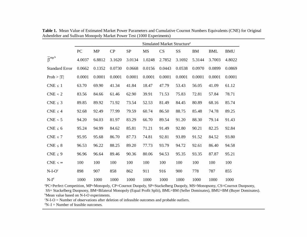
In Ashenfelter and Sullivan’s monopoly market power test, comparisons of data more than two

periods apart are excluded from the calculation of the market power parameter, identifying these pairwise

comparisons as structural shifts; thus, 4290 pairwise comparisons are omitted in each simulation. Negative

values of the market power parameter are considered to be violations of profit maximization and thus are also

excluded. Theoretically, the monopoly market power parameter ( ) should lie between zero and one,βmp

which is not the case for the mean values of calculated market power parameters for any of the ten market

structures. All results lie outside of these bounds (Table 1). For example, = 6.8812 for monopoly dataβmp

and 4.0037 for perfect competition data. The latter should theoretically be equal to zero. Ashenfelter and

Sullivan’s Cournot Numbers Equivalent (CNE), a measure of the least number of firms with Cournot

behavior that the industry could support, is calculated as . Table 1 reveals that for the monopoly market1

βmp

structure, 92.5 % of the data support the hypothesis that the industry behaves equivalent to having less than

or equal to four firms in the industry (CNE4). The cumulative percentage of the data where the CNE is less

than or equal to one, two, three, etc. should increase more rapidly with high levels of monopoly market

power exertion. For data representing market structures where low or no market power exertion is expected,

the size of the CNE should increase more slowly. This is not the case for Ashenfelter and Sullivan’s

monopoly test. For example, 93% of the perfectly competitive data support the assumption that the

industry’s behavior is equivalent to that of four Cournot firms. This result is comparable to the monopoly

result and thus inconsistent with the data.

The Lerner-type monopsonymarket power index for our monopsonymodification of Ashenfelter and

Sullivan’s original test has a lower bound of zero. Thus, the results from our implementation of the test are

consistent with theory in this respect (Table 2). For example, = 1.8355 for monopsony data and 6.8170βms

13

for perfect competition data. Note that for perfect competition should equal zero. Only 56 % of theβms

monopsony market structure data actually support a CNE of four firms, while 90 % of the monopoly and

86% of the perfect competition market structure data support a monopsonistic CNE of four firms. The

monopoly and monopsony results should be switched to lend support to the hypotheses behind the test and

the perfect competition results should be lower than the monopsonyresults. Thus, Ashenfelter and Sullivan’s

test represents an important step for deterministic nonparametric market power tests, but our study supports

Ashenfelter and Sullivan’s call for potential improvements. It is possible that information inadequately

accounted for, such as measurement errors, technological change, structural change, or input costs might

seriously bias the estimates. Additionally, the exclusion of all negative market power parameters from the

calculation of the CNE’s because they are assumed to be violations of profit maximization might be over-

restrictive. Admitting a reasonable tolerance level for small violations may improve results. The assumption

that the monopoly market power test can be generalized to industries without data on excise tax or a similar

movement in marginal cost might also be misleading.

Results for Raper, Love, and Shumway’s (1998) revision of Ashenfelter and Sullivan’s test measuring

monopoly market power exertion are reported in Table 3. Recall that Raper, Love, and Shumway explicitly

include input cost and omit obvious structural demand shifts. The mean of the monopoly market power

parameter for each market structure are indeed different from those obtained from implementation of the

original test. However, now only 79% of the data support a CNE4 for the monopoly market structure, while

96% of Cournot duopoly data and 94% of Stackelberg duopoly data support a CNE4. Additionally, the

CNE4 for perfect competition data increased to more than 95%.

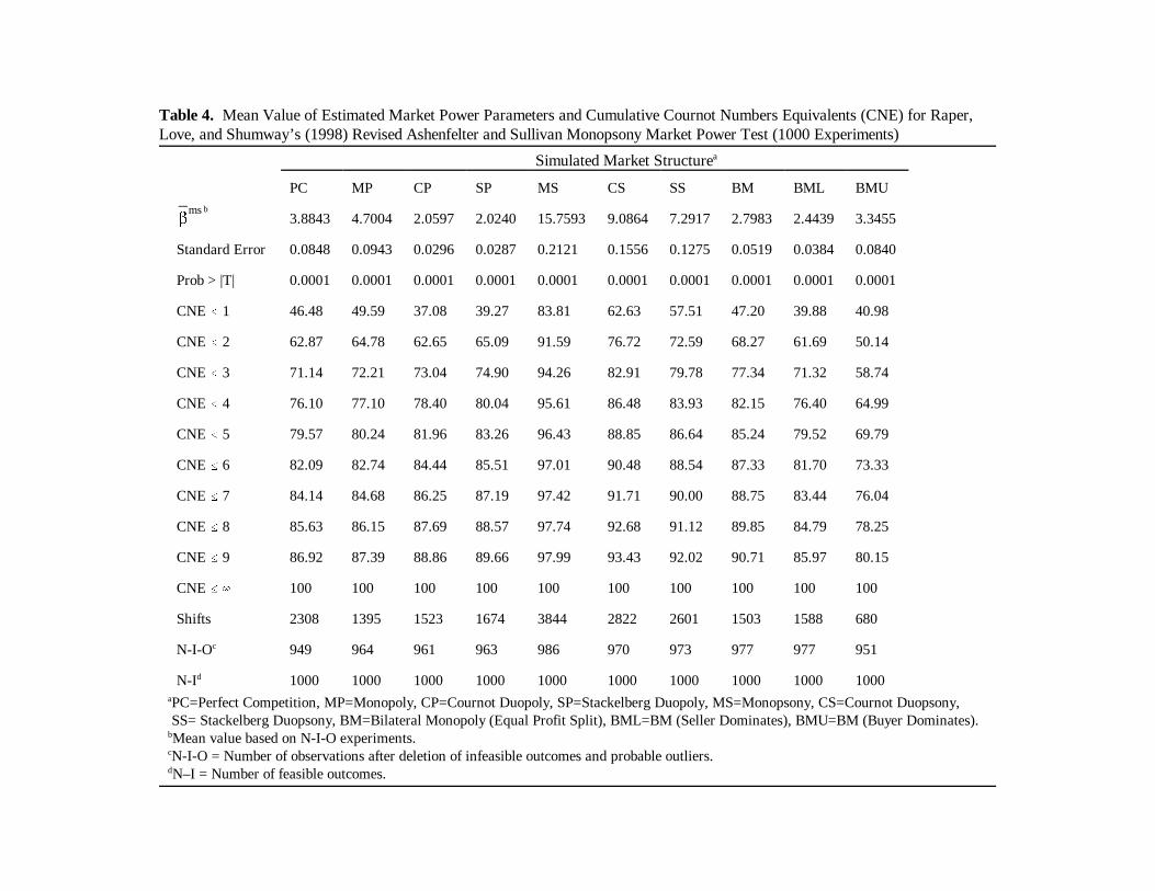
Raper, Love, and Shumway’s (1998) analagous monopsony market power test produces somewhat

more plausible results (Table 4). Again, input costs are explicitly included and obvious structural shifts in

2We realize that the choice of the weights could slightly impact the outcome of themeasures, but for simplicity in comparing to other tests, we have chosen to use one as a basevalue.

14

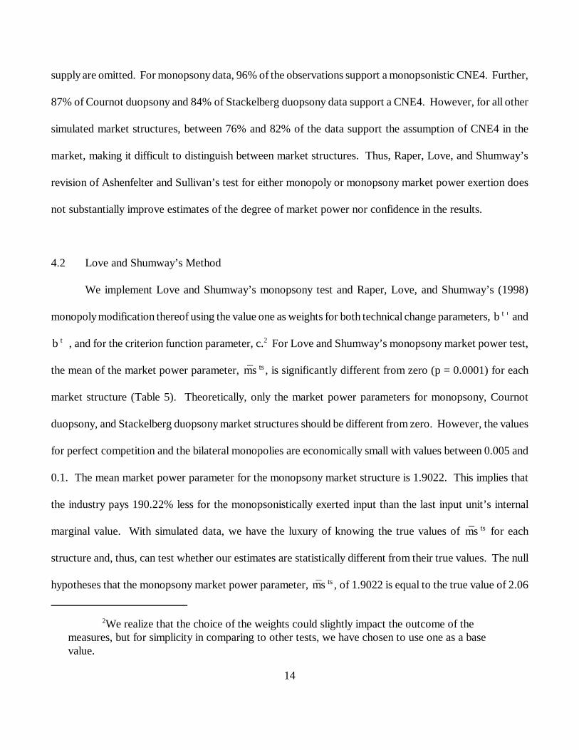
supply are omitted. For monopsony data, 96% of the observations support a monopsonistic CNE4. Further,

87% of Cournot duopsony and 84% of Stackelberg duopsony data support a CNE4. However, for all other

simulated market structures, between 76% and 82% of the data support the assumption of CNE4 in the

market, making it difficult to distinguish between market structures. Thus, Raper, Love, and Shumway’s

revision of Ashenfelter and Sullivan’s test for either monopoly or monopsony market power exertion does

not substantially improve estimates of the degree of market power nor confidence in the results.

4.2 Love and Shumway’s Method

We implement Love and Shumway’s monopsony test and Raper, Love, and Shumway’s (1998)

monopolymodification thereof using the value one as weights for both technical change parameters, andb t%

, and for the criterion function parameter, c.2 For Love and Shumway’s monopsony market power test,b t&

the mean of the market power parameter, , is significantly different from zero (p = 0.0001) for eachm̄s ts

market structure (Table 5). Theoretically, only the market power parameters for monopsony, Cournot

duopsony, and Stackelberg duopsony market structures should be different from zero. However, the values

for perfect competition and the bilateral monopolies are economically small with values between 0.005 and

0.1. The mean market power parameter for the monopsony market structure is 1.9022. This implies that

the industry pays 190.22% less for the monopsonistically exerted input than the last input unit’s internal

marginal value. With simulated data, we have the luxury of knowing the true values of for eachm̄s ts

structure and, thus, can test whether our estimates are statistically different from their true values. The null

hypotheses that the monopsony market power parameter, , of 1.9022 is equal to the true value of 2.06m̄s ts

15

for the simulated monopsony data, the Cournot of 0.3390 is equal to its true value of 0.78, and that them̄s ts

Stackelberg of 0.2462 is equal to its true value of 0.46 are all rejected with p = 0. Thus, the monopsonym̄s ts

market power test performs well in detecting the presence of monopsony market power, though less so at

distinguishing between magnitudes when market power exertion is not as extreme. However, in our

experiments the test also detects some monopsony market power when oligopolistic data are used.

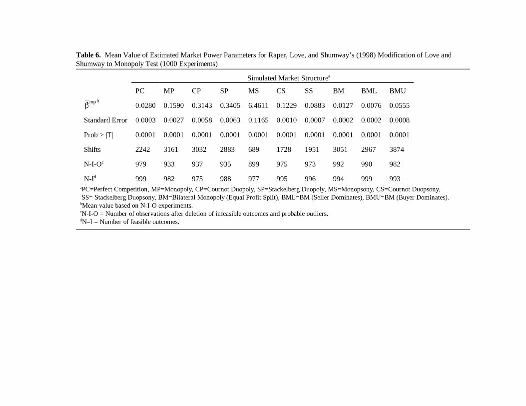
Raper, Love, and Shumway’s (1998) modification of Love and Shumway’s test which tests for

monopoly market power does not perform quite as well (Table 6). Again, mean market power parameters

for all market structures are significantly different from zero (p = 0.0001). For perfect competition, m̄p ts

= 0.028. This measure is significantly different from its true value of zero, but is economically very small and

thus not necessarily an indicator of invalidity of the test. For monopoly ( = 0.159), Cournot duopolym̄p ts

( = 0.3143), and Stackelberg duopoly data ( = 0.3405), the market power parameters are alsom̄p ts m̄p ts

significantlydifferent fromtheir true market power values of1.0, 0.5, and 0.4046 (p = 0), respectively. A m̄p ts

value of 0.4046 means that 40.46% of the output price received by the firm is monopoly markup over

marginal cost of the last unit produced. The values for Cournot duopoly and Stackelberg duopoly are

relatively large, indicating economically significant market power exertion. However, the market power

estimate for monopoly data is relatively small as compared to the duopoly cases, while for monopsonym̄p ts

isverylarge at 6.4611 and actuallyout of the theoreticalbounds. Theoreticallyit shouldbenear zero, while m̄p ts

for monopoly should be near 1.0. Monopsony, Cournot duopoly, and Stackelberg duopoly data all result

in maximum market power values of a much greater magnitude than the other market structures. Hence,

Raper, Love, and Shumway’s monopolymarket power test does appear to be able to detect monopolymarket

power exertion, though it exhibits problems in accurately detecting magnitude in our experiments. Further,

16

the market structure specification of the model is again very important as the test detects some market power

when market power is instead being exerted from the opposite party in the market.

Overall, our experiments suggest that Love and Shumway’s approach and Raper, Love, and

Shumway’s analogous monopoly test work reasonably well in identifying market power when the direction

of market power is correctly specified. However, the test appears to attribute market power in the absence

of such when market power is actually being exerted by the opposite party in the market, i.e. the test detects

monopsony power when monopoly power is instead being exerted and vice versa. This emphasizes the

importance of correctly specifying the direction of market power exertion. On the surface, this may appear

to be a simple task. However, in certain cases conditions exist for both parties of market transactions that

cloud the issue of who may hold market power. For example, many sellers organized as a cooperative to gain

bargaining power may face concentrated buyers. In such cases, Love and Shumway’s test may give an

incorrect assessment of market power exertion.

6. Conclusions

Knowledge of the degree of market power exertion is important in guiding antitrust and merger

policies. This study performs a comprehensive analysis of the relatively new approach of deterministic

nonparametric market power tests. Ashenfelter and Sullivan’s (1987) test for monopoly market power and

its counterpart for monopsonymarket power developed in this paper, as well as revisions of the test proposed

by Raper, Love, and Shumway (1998), are implemented. Additionally, Love and Shumway’s (1994)

monopsony test and Raper, Love, and Shumway’s (1998) monopoly counterpart, are implemented using

Raper, Love, and Shumway’s (1999) Monte Carlo data set that simulates data for ten different market

structures. The results are then compared to Raper, Love, and Shumway’s (1999) analysis of Bresnahan-Lau

17

type parametric market power tests for market power exertion, including monopoly, monopsony, and bilateral

market power exertion.

Ashenfelter and Sullivan make a major contribution to the field by introducing the first deterministic

nonparametric market power test. However, as they point out, their market power test might benefit from

modifications. This result is confirmed by this study. The results are not satisfactory for the original

Ashenfelter and Sullivan monopoly market power test, the analogous monopsony market power test, or

Raper, Love, and Shumway’s (1998) revisions to Ashenfelter and Sullivan for monopoly and monopsony

market power. This suggests that researchers should be hesitant about choosing Ashenfelter and Sullivan

type tests to measure the degree of market power exertion in an industry.

Love and Shumway’s approach extends Ashenfelter and Sullivan’s approach by incorporating

technical change variables and an alternative method of dealing with structural shifts. Love and Shumway’s

monopsony market power test yields estimates close to the true market power value on the downstream

firm’s side. However, to some extent the test incorrectly attributes upstream market power to downstream

firms. This implies that Love and Shumway’s monopsony market power test can be implemented under the

restriction that the model is specified for the ‘right’ direction. The monopoly market power test in Love and

Shumway’s tradition performs less accurately and should be implemented under the same restrictions. This

indicates that if there is any potential for market power from the opposing side of the market, biased results

may be obtained unless proper modifications are made.

All three parametric market power tests perform very well in Raper, Love, and Shumway’s (1999)

study. The composite model incorporates the monopoly and monopsony market power tests into one test

and performs equally as well as the unilateral monopoly and monopsony market power tests at determining

market power magnitude, when unilateral market power is present. Further, it has the advantage of

18

incorporating bilateralmarket power, thus avoiding the a priori assumption of perfectlycompetitive behavior

by one party in the transaction. This suggests that the composite model should be implemented when

choosing to perform a parametric market power test. Hyde and Perloff (1994; 1995) came to a similar

conclusion finding that even with increasing measurement error, the parametric monopsony and monopoly

market power tests find the correct market structure in virtually all of the cases. However, they also point

out that parametric market power tests may be biased when the functional form is misspecified.

The question remains as to which approach is preferred for empirical measurement of market power.

Our comparison suggests that unilateral parametric tests are more robust than unilateral deterministic

nonparametric tests to misspecification bias with respect to the direction of market power in that they do not

incorrectly attribute market power where it does not exist. However, our analysis does suggest that Love

and Shumway’s unilateralnonparametric monopsonypower test and Raper, Love, and Shumway’s monopoly

counterpart do distinguish between perfect competition and imperfect competition when market power

direction is correctly specified. Only for these two deterministic nonparametric methods do we obtain results

sufficiently close to the true value of market power exertion in the market to recommend them for use with

real data. Thus, we recommend these two deterministic market power tests as preliminary tests to specify

whether the data exhibits an economically significant amount of market power exertion. The tests may be

particularly useful in this respect since they are easily implemented and only need a small amount of data.

Consequently, if market power exertion has been found using Love and Shumway type tests, it may be

worthwhile to collect more data to implement parametric market power tests such as the composite

parametric model in Raper, Love, and Shumway (1999).

Simulated Market Structurea

PC MP CP SP MS CS SS BM BML BMUb

β̄mp

4.0037 6.8812 3.1620 3.0134 1.0248 2.7852 3.1692 5.3144 3.7003 4.8022

Standard Error 0.0662 0.1352 0.0730 0.0668 0.0156 0.0443 0.0538 0.0970 0.0899 0.0869

Prob > |T| 0.0001 0.0001 0.0001 0.0001 0.0001 0.0001 0.0001 0.0001 0.0001 0.0001

CNE # 1 63.70 69.90 41.34 41.84 18.47 47.79 53.43 56.05 41.09 61.12

CNE # 2 83.56 84.66 61.46 62.90 39.91 71.53 75.83 72.81 57.84 78.71

CNE # 3 89.85 89.92 71.92 73.54 52.53 81.49 84.45 80.89 68.16 85.74

CNE # 4 92.68 92.49 77.99 79.59 60.74 86.50 88.75 85.48 74.78 89.25

CNE # 5 94.20 94.03 81.97 83.29 66.70 89.54 91.20 88.30 79.14 91.43

CNE # 6 95.24 94.99 84.62 85.81 71.21 91.49 92.80 90.21 82.25 92.84

CNE # 7 95.95 95.68 86.70 87.73 74.81 92.81 93.89 91.52 84.52 93.80

CNE # 8 96.53 96.22 88.25 89.20 77.73 93.79 94.72 92.61 86.40 94.58

CNE # 9 96.96 96.64 89.46 90.36 80.06 94.53 95.35 93.35 87.87 95.21

CNE # 4 100 100 100 100 100 100 100 100 100 100

N-I-Oc 898 907 858 862 911 916 900 778 787 855

N-Id 1000 1000 1000 1000 1000 1000 1000 1000 1000 1000aPC=Perfect Competition, MP=Monopoly, CP=Cournot Duopoly, SP=Stackelberg Duopoly, MS=Monopsony, CS=Cournot Duopsony,SS= Stackelberg Duopsony, BM=Bilateral Monopoly (Equal Profit Split), BML=BM (Seller Dominates), BMU=BM (Buyer Dominates).

bMean value based on N-I-O experiments.cN-I-O = Number of observations after deletion of infeasible outcomes and probable outliers.dN–I = Number of feasible outcomes.

Table 1. Mean Value of Estimated Market Power Parameters and Cumulative Cournot Numbers Equivalents (CNE) for OriginalAshenfelter and Sullivan Monopoly Market Power Test (1000 Experiments)



β̄ms

6.8170 8.5815 1.9837 1.9113 1.8355 4.3288 4.9850 5.3182 2.9998 5.8255

Standard Error 0.1692 0.1876 0.0358 0.0344 0.0434 0.0925 0.1138 0.1027 0.0553 0.1288

Prob > T| 0.0001 0.0001 0.0001 0.0001 0.0001 0.0001 0.0001 0.0001 0.0001 0.0001

CNE # 1 58.07 66.43 32.27 31.94 25.75 46.81 49.99 56.82 45.78 55.63

CNE # 2 74.15 81.21 67.91 69.75 40.22 64.22 67.43 73.29 65.55 73.92

CNE # 3 81.48 87.04 81.48 82.96 49.70 73.31 76.08 81.23 74.66 81.82

CNE # 4 85.50 90.15 87.01 88.23 56.18 78.70 81.24 85.68 80.27 86.17

CNE # 5 88.18 92.07 89.93 90.94 61.07 82.28 84.52 88.42 84.04 88.75

CNE # 6 89.98 93.32 91.78 92.65 64.93 84.85 86.82 90.31 86.67 90.55

CNE # 7 91.34 94.29 93.01 93.77 68.00 86.83 88.46 91.62 88.58 91.88

CNE # 8 92.37 95.00 93.94 94.59 70.55 88.33 89.85 92.60 90.00 92.89

CNE # 9 93.19 95.52 94.63 95.23 72.79 89.55 90.85 93.40 91.09 93.69

CNE # 4 100 100 100 100 100 100 100 100 100 100

N-I-Oc 892 897 865 866 904 913 911 778 786 857



Table 2. Mean Value of Estimated Market Power Parameters and Cumulative Cournot Numbers Equivalents (CNE) forModification of Ashenfelter and Sullivan to Monopsony Market Power Test (1000 Experiments)


PC MP CPI SPI MS CSI SSI BM BML BMUb

β̄mp

4.7248 11.4490 5.1217 4.1825 1.4661 7.1698 6.7928 5.6359 3.6457 24.7017

Standard Error 0.0476 0.1169 0.0473 0.0371 0.0153 0.0723 0.0753 0.0445 0.0444 0.2273

Prob > |T| 0.0001 0.0001 0.0001 0.0001 0.0001 0.0001 0.0001 0.0001 0.0001 0.0001

CNE # 1 71.10 58.01 71.68 68.57 20.07 64.04 64.43 78.26 43.20 86.97

CNE # 2 88.97 66.99 87.71 85.16 38.38 82.74 83.19 94.32 86.29 91.55

CNE # 3 92.92 73.44 92.99 90.81 48.46 88.77 89.18 97.73 94.47 93.50

CNE # 4 94.61 79.03 95.60 93.85 55.86 91.64 92.03 98.57 97.01 94.68

CNE # 5 95.56 83.56 96.97 95.76 61.96 93.30 93.68 98.89 98.36 95.49

CNE # 6 96.18 86.98 97.73 96.91 67.00 94.40 94.75 99.08 98.91 96.10

CNE # 7 96.63 89.48 98.19 97.60 71.06 95.19 95.51 99.20 99.18 96.57

CNE # 8 96.97 91.41 98.50 98.05 74.34 95.77 96.07 99.28 99.34 96.93

CNE # 9 97.24 92.87 98.71 98.36 77.03 96.22 96.51 99.35 99.44 97.24

CNE # 4 100 100 100 100 100 100 100 100 100 100

Shifts 2242 3157 3029 2880 689 1729 1951 3051 2966 3869

N-I-Oc 976 996 999 998 990 998 993 994 986 998



Table 3. Mean Value of Estimated Market Power Parameters and Cumulative Cournot Numbers Equivalents (CNE) for Raper,Love, and Shumway’s (1998) Revised Ashenfelter and Sullivan Monopoly Market Power Test (1000 Experiments)



β̄ms

3.8843 4.7004 2.0597 2.0240 15.7593 9.0864 7.2917 2.7983 2.4439 3.3455

Standard Error 0.0848 0.0943 0.0296 0.0287 0.2121 0.1556 0.1275 0.0519 0.0384 0.0840

Prob > |T| 0.0001 0.0001 0.0001 0.0001 0.0001 0.0001 0.0001 0.0001 0.0001 0.0001

CNE # 1 46.48 49.59 37.08 39.27 83.81 62.63 57.51 47.20 39.88 40.98

CNE # 2 62.87 64.78 62.65 65.09 91.59 76.72 72.59 68.27 61.69 50.14

CNE # 3 71.14 72.21 73.04 74.90 94.26 82.91 79.78 77.34 71.32 58.74

CNE # 4 76.10 77.10 78.40 80.04 95.61 86.48 83.93 82.15 76.40 64.99

CNE # 5 79.57 80.24 81.96 83.26 96.43 88.85 86.64 85.24 79.52 69.79

CNE # 6 82.09 82.74 84.44 85.51 97.01 90.48 88.54 87.33 81.70 73.33

CNE # 7 84.14 84.68 86.25 87.19 97.42 91.71 90.00 88.75 83.44 76.04

CNE # 8 85.63 86.15 87.69 88.57 97.74 92.68 91.12 89.85 84.79 78.25

CNE # 9 86.92 87.39 88.86 89.66 97.99 93.43 92.02 90.71 85.97 80.15

CNE # 4 100 100 100 100 100 100 100 100 100 100

Shifts 2308 1395 1523 1674 3844 2822 2601 1503 1588 680

N-I-Oc 949 964 961 963 986 970 973 977 977 951



Table 4. Mean Value of Estimated Market Power Parameters and Cumulative Cournot Numbers Equivalents (CNE) for Raper,Love, and Shumway’s (1998) Revised Ashenfelter and Sullivan Monopsony Market Power Test (1000 Experiments)

23



β̄ms

0.0990 0.0780 0.1203 0.1603 1.9022 0.3390 0.2462 0.0212 0.0604 0.0045

Standard Error 0.0013 0.0009 0.0010 0.0016 0.0241 0.0047 0.0032 0.0001 0.0002 0.0001

Prob > |T| 0.0001 0.0001 0.0001 0.0001 0.0001 0.0001 0.0001 0.0001 0.0001 0.0001

Shifts 2312 1395 1524 1673 3867 2829 2605 1505 1589 681

N-I-Oc 944 954 954 944 946 953 933 959 966 954

N-Id 1000 1000 1000 1000 1000 1000 1000 1000 1000 1000aPC=Perfect Competition, MP=Monopoly, CP=Cournot Duopoly, SP=Stackelberg Duopoly, MS=Monopsony, CS=Cournot Duopsony,SS= Stackelberg Duopsony, BM=Bilateral Monopoly (Equal Profit Split), BML=BM (Seller Dominates), BMU=BM (Buyer

Dominates).bMean value based on N-I-O experiments.cN-I-O = Number of observations after deletion of infeasible outcomes and probable outliers.dN–I = Number of feasible outcomes.

Table 5. Mean Value of Estimated Market Power Parameters for Original Love and Shumway Monopsony Test (1000Experiments)



β̄mp

0.0280 0.1590 0.3143 0.3405 6.4611 0.1229 0.0883 0.0127 0.0076 0.0555

Standard Error 0.0003 0.0027 0.0058 0.0063 0.1165 0.0010 0.0007 0.0002 0.0002 0.0008

Prob > |T| 0.0001 0.0001 0.0001 0.0001 0.0001 0.0001 0.0001 0.0001 0.0001 0.0001

Shifts 2242 3161 3032 2883 689 1728 1951 3051 2967 3874

N-I-Oc 979 933 937 935 899 975 973 992 990 982



Table 6. Mean Value of Estimated Market Power Parameters for Raper, Love, and Shumway’s (1998) Modification of Love andShumway to Monopoly Test (1000 Experiments)

25

References

Afriat, Sydney N. 1972. “Efficiency Estimation of Production Functions.” International Economic Review13:568-598.

Appelbaum, Elie. 1979. “Testing Price Taking Behavior.” Journal of Econometrics 9:283-294.

Ashenfelter, Orley, and Daniel Sullivan. 1987. “Nonparametric Tests of Market Structure: An Applicationto the Cigarette Industry.” Journal of Industrial Economics 35:483-498.

Bresnahan, Timothy F. 1982. “The Oligopoly Solution Concept is Identified.” Economics Letters 10:87-92.

Chavas, Jean-Paul, and Thomas L. Cox. 1990. “A Non-Parametric Analysis of Productivity: The Case ofU.S. and Japanese Manufacturing.” American Economic Review 80:450-464.

Chavas, Jean-Paul, and Thomas L. Cox. 1992. “A Nonparametric Analysis of the Influence of Research onAgricultural Productivity.” American Journal of Agricultural Economics 74:583-591.

Chavas, Jean-Paul, and Thomas L. Cox. 1995. “On Nonparametric Supply Response Analysis.” AmericanJournal of Agricultural Economics 77:80-92.

Cox, Thomas L., and Jean-Paul Chavas. 1990. “A Nonparametric Analysis of Productivity: The Case of U.S.Agriculture.” European Review of Agricultural Economics 17:449-464.

Diewert, W. Erwin, and Celik Parkan. 1983. “Linear Programming Tests of Regularity Conditions forProduction Functions.” Pp. 131-158 in Quantitative Studies on Production and Prices, edited by W.Eichhorn, R. Henn, K. Neumann, and R.W. Shephard. Würzburg - Wien: Physica-Verlag.

Driscoll, Paul J., S. Murthy Kambhampaty, and Wayne D. Purcell. 1997. “Nonparametric Tests of ProfitMaximization in Oligopoly with Application to the Beef Packing Industry.” American Journal ofAgricultural Economics 79:872-879.

Hanoch, Giora, and Michael Rothschild. 1972. “Testing the Assumptions of Production Theory: ANonparametric Approach.” Journal of Political Economy 80:256-275.

Hyde, Charles E., and Jeffrey M. Perloff. 1994. “Can Monopsony Power be Estimated?” American Journalof Agricultural Economics 76:1151-1155.

Hyde, Charles E., and Jeffrey M. Perloff. 1995. “Can Market Power be Estimated?” Review of IndustrialOrganization 10:465-485.

26

Lambert, David K. 1994. “Technological Change in Meat and Poultry-Packing and Processing.” Journal ofAgricultural and Applied Economics 26:591-604.

Lau, Lawrence J. 1982. “On Identifying the Degree of Competitiveness from Industry Price and OutputData.” Economics Letters 10:93-99.

Lerner, Abba P. 1934. “The Concept of Monopoly and the Measurement of Monopoly Power.” Review ofEconomic Studies 1:157-175.

Love, H. Alan, and C. Richard Shumway. 1994. “Nonparametric Tests for Monopsonistic Market PowerExertion.” American Journal of Agricultural Economics 76:1156-1162.

Raper, Kellie Curry, H. Alan Love, and C. Richard Shumway. 1996. “A Nonparametric Statistical Test forMonopsony Market Power Exertion.” Selected Paper Presented at the American AgriculturalEconomics Association Annual Meeting, San Antonio, Texas. Abstract published in AmericanJournal of Agricultural Economics, 78 (December 1996):1411.

Raper, Kellie C., H. Alan Love, and C. Richard Shumway. 1998. “Distinguishing the Source of MarketPower: An Application to Cigarette Manufacturing.” Faculty Paper 98-18 , Department ofAgricultural Economics, Texas A&M University, College Station, Texas.

Raper, Kellie Curry, H. Alan Love, and C. Richard Shumway. Forthcoming. “Determining Market PowerExertion between Buyers and Sellers.” Journal of Applied Econometrics.

Ussif, Al-Amin, and David K. Lambert. 1998. “Testing for Noncompetitive Behavior in the U.S. FoodIndustry.” Selected Paper Presented at the American Agricultural Economics Association AnnualMeeting, Salt Lake City, Utah, August 2-5, 1998.

Varian, Hal R. 1984. “The Nonparametric Approach to Production Analysis.” Econometrica 52:579-597.

Varian, Hal R. 1985. “Non-Parametric Analysis of Optimizing Behavior with Measurement Error.” Journalof Econometrics 30:445 - 458.

Varian, Hal R. 1990. “Goodness-of-Fit in Optimizing Models.” Journal of Econometrics 46:125-140.

staff paper - ageconsearch.umn.eduageconsearch.umn.edu/bitstream/11757/1/sp01-53.pdfstaff paper...

Documents