1

Stat 502X Exam 1 Spring 2014

I have neither given nor received unauthorized assistance on this exam.

________________________________________________________

Name Signed Date

_________________________________________________________

Name Printed

This is a long exam consisting of 11 parts. I'll score it at 10 points per problem/part and add your best 8 scores to get an exam score (out of 80 points possible). Some parts will go faster than others, and you'll be wise to do them first.

2

1. I want to fit a function to N data pairs ,i ix y that is linear outside the interval 0,1 , is

quadratic in each of the intervals 0,.5 and .5,1 and has a first derivative for all x (has no sharp

corners). Specify below 4 functions 1 2 3 4, , , and h x h x h x h x and one linear constraint on

coefficients 0 1 2 3 4, , , , and so that the function

0 1 1 2 2 3 3 4 4y h x h x h x h x

is of the desired form.

10 pts

3

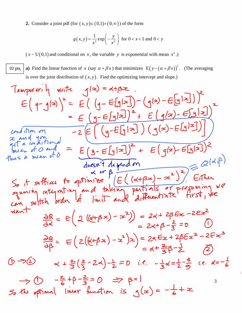
2. Consider a joint pdf (for , 0,1 0,x y ) of the form

2 2

1, exp for 0 1 and 0

yg x y x y

x x

( U 0,1x and conditional on x , the variable y is exponential with mean 2x .)

a) Find the linear function of x (say x ) that minimizes 2E y x . (The averaging

is over the joint distribution of ,x y . Find the optimizing intercept and slope.)

10 pts

4

b) Suppose that a training set consists of N data pairs ,i ix y that are independent drawn from the

distribution specified on the previous page, and that least squares is used to fit a predictor

ˆN N Nf x a b x to the training data. Suppose that it's possible to argue (don't try to do so here)

that the least squares coefficients and N Na b converge (in a proper probabilistic sense) to your

optimizers from a) as N . Then for large N , about what value of (SEL) training error do you expect to observe under this scenario? (Give a number.)

10 pts

5

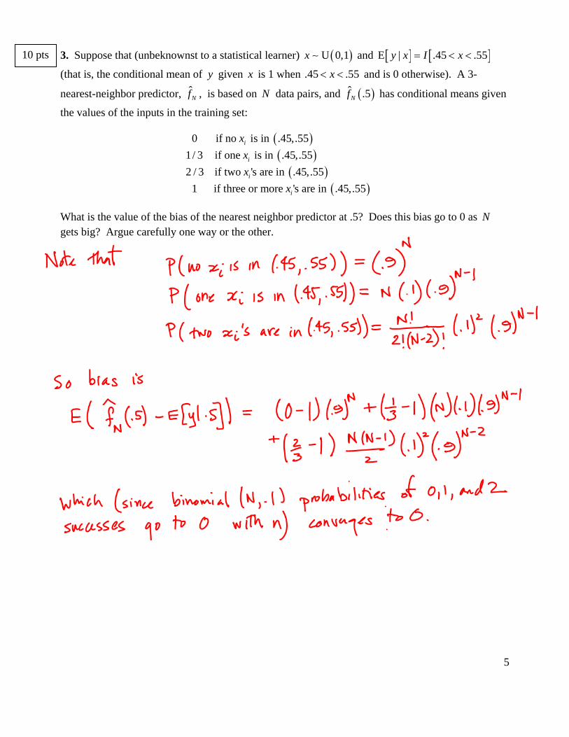
3. Suppose that (unbeknownst to a statistical learner) U 0,1x and E | .45 .55y x I x

(that is, the conditional mean of y given x is 1 when .45 .55x and is 0 otherwise). A 3-

nearest-neighbor predictor, ˆNf , is based on N data pairs, and ˆ .5Nf has conditional means given

the values of the inputs in the training set:

0 if no is in .45,.55

1/ 3 if one is in .45,.55

2 / 3 if two 's are in .45,.55

1 if three or more 's are in .45,.55

i

i

i

i

x

x

x

x

What is the value of the bias of the nearest neighbor predictor at .5? Does this bias go to 0 as N gets big? Argue carefully one way or the other.

10 pts

6

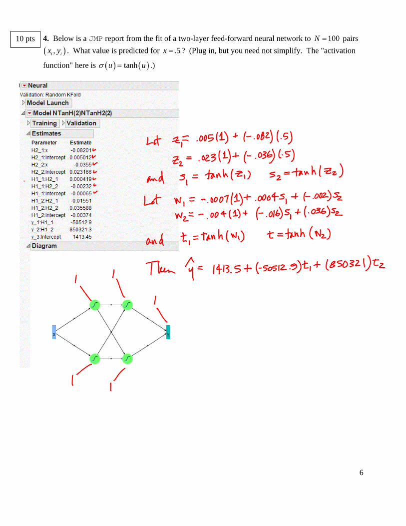
4. Below is a JMP report from the fit of a two-layer feed-forward neural network to 100N pairs

,i ix y . What value is predicted for .5x ? (Plug in, but you need not simplify. The "activation

function" here is tanhu u .)

10 pts

7

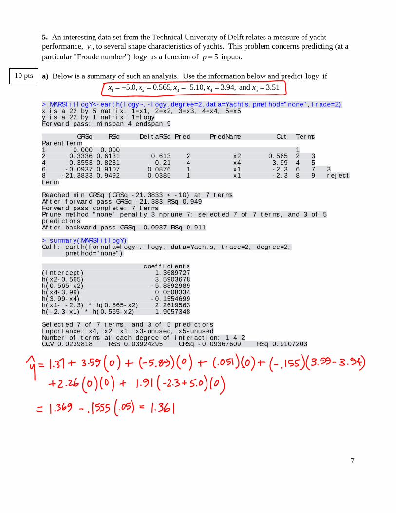
5. An interesting data set from the Technical University of Delft relates a measure of yacht performance, y , to several shape characteristics of yachts. This problem concerns predicting (at a particular "Froude number") logy as a function of 5p inputs. a) Below is a summary of such an analysis. Use the information below and predict logy if

1 2 3 4 55.0, 0.565, 5.10, 3.94, and 3.51x x x x x

> MARSfitlogY<-earth(logy~.-logy,degree=2,data=Yachts,pmethod="none",trace=2) x is a 22 by 5 matrix: 1=x1, 2=x2, 3=x3, 4=x4, 5=x5 y is a 22 by 1 matrix: 1=logy Forward pass: minspan 4 endspan 9 GRSq RSq DeltaRSq Pred PredName Cut Terms ParentTerm 1 0.000 0.000 1 2 0.3336 0.6131 0.613 2 x2 0.565 2 3 4 0.3553 0.8231 0.21 4 x4 3.99 4 5 6 -0.0937 0.9107 0.0876 1 x1 -2.3 6 7 3 8 -21.3833 0.9492 0.0385 1 x1 -2.3 8 9 reject term Reached min GRSq (GRSq -21.3833 < -10) at 7 terms After forward pass GRSq -21.383 RSq 0.949 Forward pass complete: 7 terms Prune method "none" penalty 3 nprune 7: selected 7 of 7 terms, and 3 of 5 predictors After backward pass GRSq -0.0937 RSq 0.911 > summary(MARSfitlogY) Call: earth(formula=logy~.-logy, data=Yachts, trace=2, degree=2, pmethod="none") coefficients (Intercept) 1.3689727 h(x2-0.565) 3.5903678 h(0.565-x2) -5.8892989 h(x4-3.99) 0.0508334 h(3.99-x4) -0.1554699 h(x1- -2.3) * h(0.565-x2) 2.2619563 h(-2.3-x1) * h(0.565-x2) 1.9057348 Selected 7 of 7 terms, and 3 of 5 predictors Importance: x4, x2, x1, x3-unused, x5-unused Number of terms at each degree of interaction: 1 4 2 GCV 0.0239818 RSS 0.03924295 GRSq -0.09367609 RSq 0.9107203

10 pts

8

After standardizing the 5 input variables and centering the response (for the yacht data), the following are some results from R. (The input matrix is called CX and the response vector is W .)

> round(svd(CX)$u,3) [,1] [,2] [,3] [,4] [,5] [1,] -0.029 -0.027 -0.011 0.014 -0.107 [2,] 0.239 0.222 0.003 0.336 0.479 [3,] -0.285 -0.363 -0.029 -0.376 0.631 [4,] 0.283 -0.078 -0.012 0.040 0.105 [5,] -0.407 0.061 0.006 0.020 -0.216 [6,] -0.174 0.345 0.017 0.266 0.058 [7,] 0.084 -0.341 -0.026 -0.272 0.063 [8,] 0.025 -0.047 0.012 0.230 0.166 [9,] -0.052 0.017 -0.035 -0.226 -0.027 [10,] -0.040 -0.012 -0.336 0.001 -0.127 [11,] -0.038 -0.015 0.368 -0.036 -0.107 [12,] 0.272 -0.079 -0.336 0.061 -0.061 [13,] 0.274 -0.083 0.369 0.023 -0.041 [14,] 0.339 0.108 -0.021 -0.210 -0.125 [15,] 0.027 0.196 -0.021 -0.252 -0.152 [16,] -0.111 0.529 -0.008 -0.023 0.274 [17,] -0.098 -0.206 -0.327 0.251 -0.171 [18,] -0.096 -0.210 0.378 0.214 -0.151 [19,] 0.027 0.174 -0.346 -0.254 -0.178 [20,] 0.029 0.171 0.359 -0.291 -0.158 [21,] 0.211 -0.267 -0.002 0.298 -0.082 [22,] -0.480 -0.097 -0.002 0.187 -0.072 > round(svd(CX)$v,3) [,1] [,2] [,3] [,4] [,5] [1,] -0.004 0.006 -0.999 0.047 -0.002 [2,] -0.208 -0.499 0.037 0.827 -0.150 [3,] 0.636 -0.430 -0.014 -0.210 -0.605 [4,] -0.154 -0.748 -0.024 -0.397 0.509 [5,] 0.727 0.076 0.012 0.336 0.594 > round(svd(CX)$d,3) [1] 5.970 5.579 4.583 4.132 0.397 > round(CX%*%svd(CX)$v,3) [,1] [,2] [,3] [,4] [,5] [1,] -0.175 -0.148 -0.050 0.057 -0.042 [2,] 1.425 1.240 0.014 1.388 0.190 [3,] -1.699 -2.024 -0.133 -1.554 0.251 [4,] 1.691 -0.436 -0.055 0.164 0.042 [5,] -2.429 0.342 0.028 0.081 -0.086 [6,] -1.038 1.926 0.080 1.100 0.023 [7,] 0.499 -1.904 -0.120 -1.123 0.025 [8,] 0.148 -0.260 0.054 0.950 0.066 [9,] -0.309 0.097 -0.160 -0.936 -0.011 [10,] -0.237 -0.066 -1.541 0.005 -0.050 [11,] -0.224 -0.086 1.689 -0.148 -0.043 [12,] 1.621 -0.440 -1.539 0.250 -0.024 [13,] 1.634 -0.460 1.690 0.097 -0.016 [14,] 2.026 0.602 -0.098 -0.867 -0.050 [15,] 0.163 1.093 -0.096 -1.040 -0.060 [16,] -0.660 2.951 -0.037 -0.097 0.109 [17,] -0.586 -1.150 -1.498 1.036 -0.068 [18,] -0.573 -1.171 1.732 0.883 -0.060 [19,] 0.158 0.973 -1.586 -1.049 -0.071 [20,] 0.172 0.952 1.644 -1.202 -0.063 [21,] 1.259 -1.491 -0.009 1.233 -0.033 [22,] -2.865 -0.540 -0.008 0.773 -0.029

9

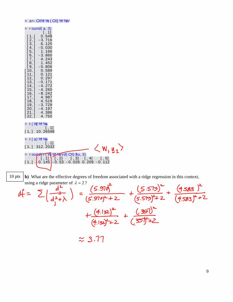
> a<-CX%*%t(CX)%*%W > round(a,3) [,1] [1,] 0.648 [2,] -3.716 [3,] 6.125 [4,] -0.030 [5,] 1.166 [6,] -3.860 [7,] 4.243 [8,] 1.452 [9,] -0.806 [10,] 0.589 [11,] 0.121 [12,] 0.297 [13,] -0.171 [14,] -4.272 [15,] -4.260 [16,] -8.242 [17,] 4.987 [18,] 4.519 [19,] -3.729 [20,] -4.197 [21,] 4.386 [22,] 4.750 > t(W)%*%a [,1] [1,] 10.26598 > t(a)%*%a [,1] [1,] 312.2032 > round(t(W)%*%svd(CX)$u,3) [,1] [,2] [,3] [,4] [,5] [1,] -0.145 -0.53 -0.026 0.209 -0.112

b) What are the effective degrees of freedom associated with a ridge regression in this context, using a ridge parameter of 2 ?

10 pts

10

c) Give the 1M component PCR and PLS vectors of predicted values PCR PLSˆ ˆ and W W .

10 pts

11

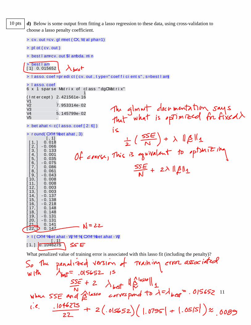
d) Below is some output from fitting a lasso regression to these data, using cross-validation to choose a lasso penalty coefficient.

> cv.out=cv.glmnet(CX,W,alpha=1) > plot(cv.out) > bestlam=cv.out$lambda.min > bestlam [1] 0.015652 > lasso.coef=predict(cv.out,type="coefficients",s=bestlam) > lasso.coef 6 x 1 sparse Matrix of class "dgCMatrix" 1 (Intercept) 2.421561e-16 V1 . V2 7.953314e-02 V3 . V4 5.145799e-02 V5 . > betahat<-c(lasso.coef[2:6]) > round(CX%*%betahat,3) [,1] [1,] 0.018 [2,] -0.066 [3,] 0.133 [4,] 0.001 [5,] 0.035 [6,] -0.075 [7,] 0.086 [8,] 0.061 [9,] -0.043 [10,] 0.008 [11,] 0.008 [12,] 0.003 [13,] 0.003 [14,] -0.137 [15,] -0.138 [16,] -0.218 [17,] 0.148 [18,] 0.148 [19,] -0.131 [20,] -0.131 [21,] 0.141 [22,] 0.147 > t(CX%*%betahat-W)%*%(CX%*%betahat-W) [,1] [1,] 0.1046275

What penalized value of training error is associated with this lasso fit (including the penalty)?

10 pts

12

6. Below is a particular smoother matrix, S , for 1p data at values 0,.1,.2,.3, ,.9,1.0x (The

labeling convention used below is 1 2 3 110, .1, .2, , 1.0x x x x .)

[,1] [,2] [,3] [,4] [,5] [,6] [,7] [,8] [,9] [,10] [,11] [1,] 0.721 0.265 0.013 0.000 0.000 0.000 0.000 0.000 0.000 0.000 0.000 [2,] 0.210 0.570 0.210 0.010 0.000 0.000 0.000 0.000 0.000 0.000 0.000 [3,] 0.010 0.208 0.564 0.208 0.010 0.000 0.000 0.000 0.000 0.000 0.000 [4,] 0.000 0.010 0.208 0.564 0.208 0.010 0.000 0.000 0.000 0.000 0.000 [5,] 0.000 0.000 0.010 0.208 0.564 0.208 0.010 0.000 0.000 0.000 0.000 [6,] 0.000 0.000 0.000 0.010 0.208 0.564 0.208 0.010 0.000 0.000 0.000 [7,] 0.000 0.000 0.000 0.000 0.010 0.208 0.564 0.208 0.010 0.000 0.000 [8,] 0.000 0.000 0.000 0.000 0.000 0.010 0.208 0.564 0.208 0.010 0.000 [9,] 0.000 0.000 0.000 0.000 0.000 0.000 0.010 0.208 0.564 0.208 0.010 [10,] 0.000 0.000 0.000 0.000 0.000 0.000 0.000 0.010 0.210 0.570 0.210 [11,] 0.000 0.000 0.000 0.000 0.000 0.000 0.000 0.000 0.013 0.265 0.721

What effective degrees of freedom are associated with this smoother?

Approximately what bandwith is associated with this smoother?

For training data as below, what is ˆ .4f ?

y 1 3 2 4 2 6 7 9 7 8 6

x 0 .1 .2 .3 .4 .5 .6 .7 .8 .9 1.0

10 pts

13

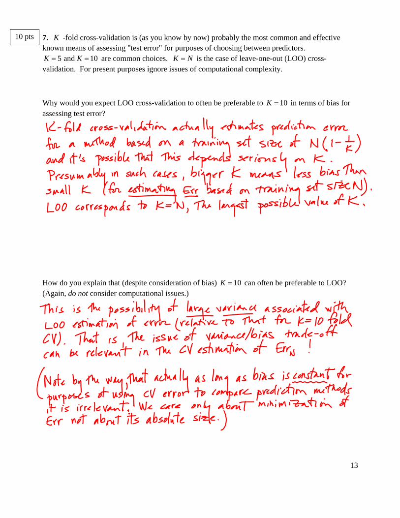
7. K -fold cross-validation is (as you know by now) probably the most common and effective known means of assessing "test error" for purposes of choosing between predictors.

5 and 10K K are common choices. K N is the case of leave-one-out (LOO) cross-validation. For present purposes ignore issues of computational complexity.

Why would you expect LOO cross-validation to often be preferable to 10K in terms of bias for assessing test error?

How do you explain that (despite consideration of bias) 10K can often be preferable to LOO? (Again, do not consider computational issues.)

10 pts