State Estimation for Hybrid Systems: Applications to Aircraft

Tracking ∗

Inseok Hwang∗, Hamsa Balakrishnan†, and Claire Tomlin†

∗School of Aeronautics and Astronautics, Purdue University, IN 47907† Dept. of Aeronautics and Astronautics, Stanford University, CA 94305

ihwang@purdue.edu, {hamsa,tomlin}@stanford.edu

Abstract

The problem of estimating the discrete and continuous state of a stochastic lin-

ear hybrid system, given only the continuous system output data, is studied. Well

established techniques for hybrid estimation, known as the Multiple Model Adaptive

Estimation algorithm, and the Interacting Multiple Model algorithm, are first reviewed.

Conditions that must be satisfied in order to guarantee the convergence of these hybrid

estimation algorithms are then presented. These conditions also provide a means to

predict, as a function of the system parameters, which transitions in a hybrid system

are relatively easy to detect. A new variant of hybrid estimation algorithms, called the

Residual-Mean Interacting Multiple Model (RMIMM) algorithm, is then proposed and

analyzed. The performance of RMIMM is demonstrated through multi-modal aircraft

trajectory tracking examples.

1 Introduction

Hybrid systems are dynamical systems that combine continuous dynamics modeled by dif-

ferential (or difference) equations and discrete dynamics modeled by finite automata. Since

hybrid systems can suitably model the complex behavior of varied embedded control sys-

tems, such as robotic, transportation, and process control systems, there has been consid-

erable interest in the estimation and control of hybrid systems among researchers in both

academic and industrial communities [1, 2, 3, 4]. The objective of hybrid estimation is to

compute both the discrete and continuous state estimates of a hybrid system at any given

time. Hybrid estimators usually consist of the combination of a bank of continuous state

∗This research was supported by ONR under MURI contract N00014-02-1-0720, by NASA JUP undergrant NAG2-1564, by NASA grant NCC2-5536, and by an NSF Career Award (ECS-9985072). H. Balakr-ishnan was supported by a Stanford Graduate Fellowship.

1

2

estimators, each one designed for a different discrete state, or mode, and a mode selecting

algorithm. How the correct mode is selected depends on the type of output data available.

The hybrid estimators analyzed in this paper address a particularly challenging problem –

that of mode and continuous state estimation given only the observation of the continuous

state. In this case, the hybrid estimators use the differences in statistical properties (such as

mean and covariance) of the outputs of the different continuous state estimators to choose

the correct mode.

In air traffic surveillance, the accurate tracking of aircraft is important because all traffic

advisories are based on the current state estimates of the aircraft. In this domain, the

observations correspond to radar measurements of the positions of the aircraft (observation

of the continuous state). The flight mode of the aircraft, indicating, for example, constant

velocity straight flight, or coordinate turn, is not observed. Yet knowledge of the flight mode

would be valuable to a surveillance system, as it is one of the strongest indicators of the

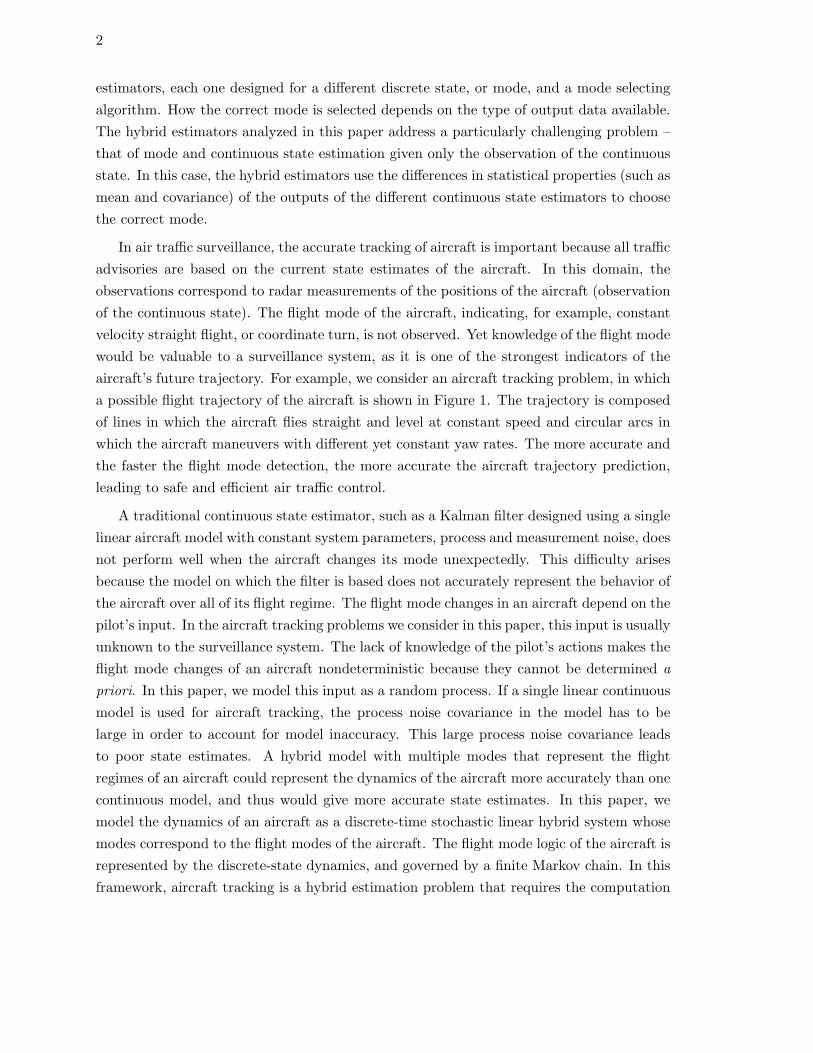
aircraft’s future trajectory. For example, we consider an aircraft tracking problem, in which

a possible flight trajectory of the aircraft is shown in Figure 1. The trajectory is composed

of lines in which the aircraft flies straight and level at constant speed and circular arcs in

which the aircraft maneuvers with different yet constant yaw rates. The more accurate and

the faster the flight mode detection, the more accurate the aircraft trajectory prediction,

leading to safe and efficient air traffic control.

A traditional continuous state estimator, such as a Kalman filter designed using a single

linear aircraft model with constant system parameters, process and measurement noise, does

not perform well when the aircraft changes its mode unexpectedly. This difficulty arises

because the model on which the filter is based does not accurately represent the behavior of

the aircraft over all of its flight regime. The flight mode changes in an aircraft depend on the

pilot’s input. In the aircraft tracking problems we consider in this paper, this input is usually

unknown to the surveillance system. The lack of knowledge of the pilot’s actions makes the

flight mode changes of an aircraft nondeterministic because they cannot be determined a

priori. In this paper, we model this input as a random process. If a single linear continuous

model is used for aircraft tracking, the process noise covariance in the model has to be

large in order to account for model inaccuracy. This large process noise covariance leads

to poor state estimates. A hybrid model with multiple modes that represent the flight

regimes of an aircraft could represent the dynamics of the aircraft more accurately than one

continuous model, and thus would give more accurate state estimates. In this paper, we

model the dynamics of an aircraft as a discrete-time stochastic linear hybrid system whose

modes correspond to the flight modes of the aircraft. The flight mode logic of the aircraft is

represented by the discrete-state dynamics, and governed by a finite Markov chain. In this

framework, aircraft tracking is a hybrid estimation problem that requires the computation

3

−15 −10 −5 0 5 10 1510

15

20

25

30

35

40Flight trajectory

x−position [km]

y−po

sitio

n [k

m]

Figure 1: An aircraft trajectory.

of both the continuous state and discrete mode estimates. Therefore, in this paper, we

consider a class of hybrid systems, called discrete-time stochastic linear hybrid systems,

which have continuous dynamics modeled by linear difference equations and discrete-state

dynamics modeled by a finite Markov chain.

1.1 Related Work

Hybrid estimation algorithms have been developed for discrete-time stochastic linear hybrid

systems in which the mode transitions are governed by finite-state Markov chains. The

Multiple Model Adaptive Estimation (MMAE) algorithm [5] is an algorithm in which,

during hypothesis testing, the residuals of the different Kalman filters for each mode are

used to form functions that reflect the likelihood that estimates of each of the different

modes is the correct one. These functions, called likelihood functions, serve as adaptive

weights, and the state estimate is the weighted sum of the state estimates computed by

individual Kalman filters. In MMAE, the individual Kalman filters matched to the different

modes run independently. In the Interacting Multiple Model (IMM) algorithm [6] which is

a refinement of MMAE, a set of mode-matched Kalman filters interact with each other by

using combinations of previous estimates computed by individual Kalman filters as initial

conditions for each of the Kalman filters at every time step. The original rationale behind

this refinement was to reduce the exponential complexity O(NT ) of the optimal hybrid

estimator which minimizes the mean-square estimation error (where N is the number of

modes and T is the total number of time samples) to O(N). Maybeck [5], Bar-Shalom et

4

al. [6], Sworder and Boyd [7], and Hawkes and Moore [8] describe several similar hybrid

estimation algorithms and their applications.

The performance of such hybrid estimators has been studied for several decades. Mag-

ill [9] provided sufficient conditions for the convergence of the adaptive weight for the correct

mode to unity. These conditions are valid for the hybrid estimation of a specific class of

systems, in which a constant parameter vector is unknown and the continuous dynamics in

each mode has a single output. Lainiotis et al. [10, 11, 12] extended these results to systems

with multiple outputs, and derived the recursive form of the optimal adaptive estimator as

well as its exact error covariance. Hawkes et al. [8] examined the asymptotic behavior of the

adaptive weights which determine the performance of hybrid estimation algorithms. Many

other approaches to the performance analysis of hybrid estimation, in which hypothesis

testing is performed using adaptive weights, can be found in the work of Hawkes et al. [8],

and the references therein. Baram et al. [13, 14] provided conditions under which, for a set

of systems driven by stationary white Gaussian inputs and no discrete transitions, the mode

probability of the true model converges to unity, i.e., the probability that the estimated

model is the true model converges asymptotically to unity. However, the system studied

by Baram et al. [13, 14] is a set of stochastic, stationary Gaussian models which run inde-

pendently. Thus, the conditions derived in [13, 14] are more relevant to the observability

of stochastic linear hybrid systems [15]. Caputi [16] derived a necessary condition for the

convergence of hybrid estimation algorithms through the analysis of steady state residuals,

and showed that the performance of the hybrid estimator depends on the DC gain of the

continuous dynamics. This condition is only valid for a specific class of hybrid systems, in

which the continuous dynamics for all the modes is the same, but the inputs are distinct

and consist of a constant bias vector and zero-mean white Gaussian random noise.

The researchers cited above have analyzed hybrid estimation in several special classes of

systems, yet general analysis techniques for evaluating the performance of hybrid estimation

algorithms for stochastic linear hybrid systems have not been investigated in detail. In

this paper, we analyze the properties of hybrid estimation algorithms for stochastic linear

hybrid systems and derive conditions under which the computed hybrid estimates converge

exponentially to the exact hybrid states. We say that a mode transition is more detectable

than another if the time taken for the mode estimate to converge to the true mode is less

for the former transition than for the latter. The results of this analysis give some insight

into which mode transitions are more detectable than others and also into how to improve

the performance of hybrid estimators. We then show analytically why the IMM algorithm,

which has been widely and successfully used in the area of multiple target tracking, has

better performance than the MMAE algorithm. Using the results of this performance

analysis of hybrid estimation algorithms, we propose a modified IMM algorithm, called the

5

Residual-Mean Interacting Multiple Model (RMIMM) algorithm, which uses the mean of

the residual produced by each Kalman filter, producing better mode estimates as well as

continuous state estimates than the standard IMM algorithm. We return to the aircraft

tracking example to demonstrate the effectiveness of RMIMM.

This paper is organized as follows: Section 2 presents the structure of a stochastic

linear hybrid system and problem statements. In Section 3, we describe a generic hybrid

estimation algorithm, which could be MMAE, IMM, or any other refinement of the basic

hybrid estimation algorithm. In Section 4, we analyze the performance of hybrid estimation

algorithms and derive upper bounds for the mode estimation delay, as well as conditions

that guarantee the exponential convergence of hybrid estimation algorithms. Section 4 also

presents a comparison of the performance of different hybrid estimation algorithms. In

Section 5, we derive the RMIMM algorithm and demonstrate its performance through a

maneuvering aircraft tracking example.

2 Discrete-time stochastic linear hybrid systems

We consider a discrete-time stochastic linear hybrid system

H :

{

x(k + 1) = Aix(k) + Biu(k) + wi(k)

z(k) = Cix(k) + vi(k)(1)

where k ∈ N, x ∈ Rn, u ∈ R

l and z ∈ Rp are the continuous state, control input, and output

variables respectively. The index i ∈ {1, 2, · · · , N} represents the mode whose evolution is

governed by the finite state Markov chain

µ(k + 1) = Πµ(k) (2)

where Π = {πij} ∈ RN×N is the mode transition matrix and µ(k) ∈ R

N is the mode

probability at time k. The system matrices Ai ∈ Rn×n, Bi ∈ R

n×l, and Ci ∈ Rp×n

for i ∈ {1, 2, · · · , N} are assumed known. We denote the covariance of the initial state

x(k0) as π0 ∈ RN , and assume that the process noise wi(k) and the measurement noise

vi(k) are uncorrelated, zero-mean white Gaussian sequences with the covariance matrices

E[wi(k)wi(k)T ] = Qi ∈ Rn×n and E[vi(k)vi(k)T ] = Ri ∈ R

p×p respectively. E[·] and (·)T

denote expectation and matrix transpose respectively. It is assumed that wi(k) and vi(k)

are both uncorrelated with the initial state, i.e., E[x(k0)wi(k)T ] = E[x(k0)vi(k)T ] = 0. We

define Z(k) = {z(0), · · · , z(k)} as the measurement sequence up to time k. Since the state

evolution of a hybrid system has continuous trajectories as well as discrete jumps, we define

a hybrid time trajectory:

6

Definition 2.1 (Hybrid time trajectory) A hybrid time trajectory is a sequence of intervals

[k0, k1 − 1][k1, k2 − 1] · · · [ki, ki+1 − 1] · · · where ki(i ≥ 1) is the time at which the i-th mode

transition occurs.

From the above definition, the sojourn time is defined as the time spent by the hybrid

system between discrete state transitions. In this paper, by ‘exponential convergence of a

hybrid estimator’ we mean:

Definition 2.2 (Exponential convergence of a hybrid estimator) Given a hybrid system

H with N modes, we say that a hybrid estimator is exponentially convergent if its mode

estimate exhibits correct identification of the mode transition sequence of the original system

in a finite number of steps; the continuous state estimate at any instant has a unique mean

and convergent covariance in the sense of the minimum mean square error; and the mean

of the continuous state estimation error converges exponentially to the given steady-state

error bound.

Definition 2.2 indicates the fact that a hybrid estimator converges exponentially only if the

divergence of the mean of the continuous state estimation error when the mode estimate is

incorrect does not destroy the exponential convergence of the mean of the estimation error

when the mode estimate is correct.

In this paper, through the performance analysis of hybrid estimation algorithms, we

address interesting problems: under what conditions the states estimates converge expo-

nentially to the true states; how fast hybrid estimation algorithms can correctly detect mode

transitions; and which mode transitions are easier to detect than others. Based on these

analysis results, a new variant of hybrid estimation algorithms is proposed.

3 Hybrid estimation algorithms

In this section, we consider a generic hybrid estimation algorithm [5] for the discrete-time

stochastic linear hybrid system (1)-(2). As seen in Section 1, such an algorithm typically

contains a set of Kalman filters matched to the different modes of the hybrid system.

Following the Bayesian estimation derivation in [5], the continuous state estimate is the

conditional mean:

x(k + 1) = E[x(k + 1)|Z(k + 1)] =

∫ ∞

−∞x(k + 1)p(x(k + 1)|Z(k + 1))dx(k + 1) (3)

where p(·|·) is the conditional probability density function, given by:

p(x(k + 1)|Z(k + 1)) =N∑

i=1

p(x(k + 1), Z(k + 1), mi(k + 1))

p(Z(k + 1))

7

and mi(k + 1) denotes the event that the mode at time k + 1 is i. Then, the state estimate

(3) is

x(k + 1) =N∑

i=1

xi(k + 1)p(mi(k + 1)|Z(k + 1)) (4)

where xi(k + 1) =∫∞−∞ x(k + 1)p(x(k + 1)|Z(k + 1), mi(k + 1))dx(k + 1) is the mode-

conditioned state estimate of x(k +1), which is the state estimate based on the assumption

that the mode at time k + 1 is mi(k + 1) and is computed by the state estimator (in this

paper, a Kalman filter) matched to mode i. Therefore, the state estimate (4) is a weighted

sum of N mode-conditioned state estimates produced by each Kalman filter with the weight

p(mi(k + 1)|Z(k + 1)). The weight is given by

p(mi(k + 1)|Z(k + 1)) =Λi(k + 1)p(mi(k + 1)|Z(k))

p(z(k + 1)|Z(k))(5)

where Λi(k + 1) := N (ri(k + 1); 0, Si(k + 1)) is the likelihood function of mode i.

ri(k+1) = z(k+1)−Cixi(k+1|k) is the residual produced by Kalman filter i, Si(k+1) ∈ Rp×p

is the corresponding residual covariance, xi(k + 1|k) is the state estimate by Kalman filter

i at time k + 1 before the measurement update, and N (a; b, c) is the probability at a of a

normal distribution with mean b and covariance c. p(mi(k+1)|Z(k)) is the mode probability

estimate at time k + 1. If the mode transitions are governed by a finite Markov chain, the

mode probability estimate can be expressed by

p(mi(k + 1)|Z(k)) =N∑

l=1

πilp(ml(k)|Z(k)) (6)

Thus, the weight (5) is

p(mi(k + 1)|Z(k + 1)) =Λi(k + 1)

c(k + 1)

N∑

l=1

πilp(ml(k)|Z(k)) := µi(k + 1) (7)

where c(k + 1) is a normalization constant. µi(k + 1) in (7) denotes the probability of

mode i at time (k + 1). The mode estimate at time k is chosen to be the mode which has

the maximum mode probability at that time. The mode probability depends not only on

the finite Markov chain (discrete dynamics) but also on the likelihood produced by each

Kalman filter (continuous dynamics). The state estimate (4) is

x(k + 1) =N∑

i=1

xi(k + 1)[Λi(k + 1)

c(k + 1)

N∑

l=1

πilp(ml(k)|Z(k))]

(8)

8

Equations (7)-(8) are the core of the Multiple Model Adaptive Estimation (MMAE) algo-

rithm [5]. In MMAE, all individual Kalman filters run independently at every time step.

Equations (7)-(8) show that the state estimate depends on the likelihood function; the

performance of the hybrid estimator thus greatly depends on the behavior of the likeli-

hood function. A variant of MMAE, the Interacting Multiple Model (IMM) algorithm [18]

Figure 2: Structure of the IMM algorithm (two-mode system) from [17]

(on which RMIMM is based) has the same structure as MMAE except that it has a Mix-

ing/Interacting step at the beginning of the estimation process, which computes new initial

conditions for the Kalman filters matched to the individual modes at each time step. Figure

2 shows a schematic of the IMM algorithm for a system with two discrete modes. The IMM

algorithm uses a bank of Kalman filters (KF1 and KF2) and computes the mode probabil-

ities µi(k + 1) and the continuous state estimate x(k + 1) in the same way as MMAE does

in (7) and (8) respectively. However, individual Kalman filters share information about the

other Kalman filters through new initial conditions (x0i(k), P0i(k) (i = 1,2)) at each time

step. The components of IMM in Figure 2 are defined as follows:

1. Mixing probability: This is the probability that the system is in mode i at time k,

given that it is in mode j at time k + 1 (i, j ∈ {1, · · · , N}):

µij(k|k) =1

cjπjiµi(k) (9)

9

where cj is a normalization constant, and where µi(k) is the mode probability of mode

i at time k, i.e., a measure of how probable it is that the system is in mode i at time k.

The initial condition µi(0) is assumed given, and is usually obtained from properties

of the system.

2. New initial states and covariances: The input to each Kalman filter is adjusted

by weighting the output of each Kalman filter with the mixing probability as the

weight:

x0j(k) =N∑

i=1

xi(k)µij(k|k)

P0j(k) =N∑

i=1

[Pi(k) + [xi(k)−x0j(k)] × [xi(k)−x0j(k)]T]

µij(k|k)

where xi(k) and Pi(k) are the state estimate and its covariance produced by Kalman

filter i after the measurement update at time k.

3. Kalman Filter: N Kalman filters run in parallel (multiple-model-based (hybrid)

estimation).

4. Mode likelihood functions: The likelihood function of mode j is a measure of how

likely it is that the model used in Kalman filter j is the correct one; it is computed

with the residual and its covariance produced by Kalman filter j:

Λj(k + 1) = N (rj(k + 1); 0, Sj(k + 1)) (10)

where rj(k + 1) := z(k + 1) − Cj xj(k + 1|k) is the residual of Kalman filter j and

Sj(k + 1) is its covariance.

5. Mode probabilities: The probability of mode j is a measure of how probable it is

that the system is in mode j:

µj(k + 1) =1

c(k + 1)Λj(k + 1)

N∑

i=1

πjiµi(k) (11)

where c(k + 1) is a normalization constant. The probability of each mode is updated

using the likelihood function.

6. Combination (output of the IMM algorithm): The state estimate is a weighted

sum of the estimates from N Kalman filters and the mode estimate is the mode which

10

has the highest mode probability:

x(k + 1) =∑N

j=1 xj(k + 1)µj(k + 1)

P (k + 1) =∑N

j=1{Pj(k + 1) + [xj(k + 1) − x(k + 1)][xj(k + 1) − x(k + 1)]T }µj(k + 1)

m(k + 1) = arg maxj µj(k + 1)

(12)

where m(k + 1) is the mode estimate at time k + 1.

In the next section, we investigate the performance of hybrid estimation algorithms such as

MMAE and IMM in detail.

4 Performance analysis of the hybrid estimation algorithm

In this section, we first analyze the performance of the hybrid estimation algorithm (either

MMAE or IMM) by analyzing the steady-state mean residuals. Since steady-state analysis

gives only necessary conditions on the performance of hybrid estimation, we then analyze

the transient behavior of mode probabilities, which are functions of the likelihoods and

therefore of the residuals.

4.1 Performance derived from steady-state analysis

Motivated by Caputi [16], we derive the steady-state mean residual for each mode i for the

hybrid system (1)-(2). We define:

∆Ai := AT − Ai, ∆Bi := BT − Bi

∆Ci := CT − Ci, xiss := limk→∞ xi(k)

∆uiss := uTss− uiss := limk→∞ uT (k) − limk→∞ ui(k)

eiss := limk→∞ E[ei(k)] = limk→∞ E[(x(k) − xi(k))]

where the subscript T ∈ {1, · · · , N} represents the true mode. The mean residual and the

mean estimation error of the filter i (i 6= T ) at time k are

ri(k) = CT AT ei(k − 1) + (CT ∆Ai + ∆CiAT − ∆Ci∆Ai)xi(k − 1)

+(CT ∆Bi + ∆CiBT − ∆Ci∆Bi)u(k − 1)

ei(k) = (I − KiCT )AT ei(k − 1) + ((I − KiCT )∆Ai − Ki∆CiAi)xi(k − 1)

+((I − KiCT )∆Bi − Ki∆CiBi)u(k − 1)

11

The steady-state mean residual for mode i is

riss := limk→∞ ri(k)

= (CT AT Θ((I − KiCT )∆Ai − Ki∆CiAi)) + (CT ∆Ai + ∆CiAT − ∆Ci∆Ai))xiss

+(CT AT Θ(I − KiCT )BT + CT BT )∆uiss + (CT AT Θ((I − KiCT )∆Bi − Ki∆CiBi)

+(CT ∆Bi + ∆CiBT − ∆Ci∆Bi))uiss

where Θ := (I − (I − KiCT )AT )−1 and Ki is the steady-state Kalman filter gain for mode

i. We assume that Θ is invertible. If mode i is the correct mode (i = T ), then riss = 0.

If rjss 6= 0 (∀j 6= i), then the correct mode can be detected because only the steady-state

mean residual of the true mode is zero, and those of the other modes are not zero. However,

even if mode i is not the correct mode (i 6= T ), the steady-state mean residual for mode i

is zero if all of the following equalities are satisfied:

(I − KiCT )∆Ai − Ki∆CiAi = 0

(CT ∆Ai + ∆CiAT − ∆Ci∆Ai) = 0

(I − KiCT )∆Bi − Ki∆CiBi = 0

(CT ∆Bi + ∆CiBT − ∆Ci∆Bi) = 0

∆uiss = 0

This means that if at least two models are identical and the corresponding control inputs

are the same, then the steady-state residuals of both the corresponding modes are zero. In

this case, the hybrid estimator cannot uniquely determine the correct mode. In other words,

the performance of the hybrid estimation algorithm depends on the differences between the

residuals which in turn arise from model differences and input differences. In the above

condition, the first four equalities come from model differences and the last equality comes

from input differences. This analysis result supports Maybeck’s observation that the per-

formance of MMAE depends on a significant difference between the residual characteristics

[5].

4.2 Performance derived from transient analysis

We now consider the transient mean behavior of a hybrid estimator, and analyze its per-

formance in the sense of exponential convergence in Definition 2.2. A steady-state Kalman

filter is assumed to be used as the state estimator for each mode. For the sake of notational

simplicity, we define µ−i (k) :=

∑Nl=1 πilµl(k − 1). The condition for correct mode detection

at time k is:

µT (k) > µi(k), ∀i 6= T (13)

12

Using µi(k) := p(mi(k)|Z(k)) from (7) and

Λi(k) = N (ri(k); 0, Si) := (2π)−n/2|Si|−1 exp[−1

2ri(k)T S−1

i ri(k)]

in (5), where Si = STi > 0 and r is the mean residual, (13) becomes

0 ≤ rT (k)T S−1T rT (k) < ri(k)T S−1

i ri(k) + 2 ln

( |Si||ST |

)

+ 2 ln

(

µ−T (k)

µ−i (k)

)

(14)

To detect the correct mode exactly for any k ∈ N, (14) must hold for all k ∈ N (∀i 6= T ). If

there is a time delay (δT ) for correct mode detection when a mode transition into mode T

occurs at time kl (l ∈ N+), (14) holds for k ∈ [kl + δT , kl+1). For the existence of an rT (k)

satisfying (14), using the properties of the eigenvalues of positive definite matrices [19], we

derive the following:

Proposition 4.1 The correct mode can be detected in at most δT time steps after a mode

transition at time kl if there exists δT ∈ N+ such that for k ∈ [kl + δT , kl+1) (l ∈ N

+,

∀i 6= T ), Condition 1 holds, and either Condition 2 or Condition 3 is true.

1. ri(k)T S−1i ri(k) + 2

[

ln(

|Si||ST |

)

+ ln(

µ−

T(k)

µ−

i (k)

)

]

> 0

2. rT (k)T S−1T rT (k) < ri(k)T S−1

i ri(k) + 2[

ln(

|Si||ST |

)

+ ln(

µ−

T(k)

µ−

i (k)

)

]

3. ‖rT (k)‖2 <λmin(S−1

i )

λmax(S−1

T)‖ri(k)‖2 + 2

λmax(S−1

T)

[

ln(

|Si||ST |

)

+ ln(µ−

T(k)

µ−

i (k)

)

]

Conditions 1 and 2 indicate that the probability of the true mode should be greater than

those of the other modes for correct mode detection. Since Condition 3 is obtained by

considering the worst case, i.e., when the upper bound on the left-hand side of the inequal-

ity in Condition 2 is less than the lower bound on the right-hand side, Condition 3 is a

sufficient condition for correct mode detection, and might be very conservative. However,

it gives valuable insight into the performance of hybrid estimation. Fast mode detection

is dependent not only on the magnitudes of the residuals produced by each Kalman filter

but also on the residual covariances. Ifλmin(S−1

i )

λmax(S−1

T)

is small and/or |Si||ST | is small, it is difficult

for Condition 3 to hold and thus to detect the correct mode. Therefore, by checking the

eigenvalues and determinant of S−1i , we can tell which mode transitions are more detectable

than the others. This is similar to the idea of the observability grammian as a measure of

which states are more observable than others [20]. If we consider the steady-state residual

mean, Condition 3 becomes, ∀i 6= T ,

‖rTss‖2 <

λmin(S−1i )

λmax(S−1T )

‖riss‖2 +2

λmax(S−1T )

[

ln

( |Si||ST |

)

+ ln(µ−

Tss

µ−iss

)]

(15)

13

Therefore, if the asymptotic behavior of the residuals satisfies (15) and the sojourn timesare long enough for the residuals to converge to their steady-state values, then MMAE is

guaranteed to estimate the hybrid states correctly.

We now derive the mode estimation delay δi using Condition 3 in Proposition 4.1. The

mean residual of the correct filter at time kl + δi (l ∈ N+), when i = T , is rT (kl + δT ) =

CT AT [(I − KT CT )AT ]δT−1eT (kl), where eT (kl) is the mean of the estimation error of the

correct filter at time kl. For the sake of notational simplicity, we define

FT := (I − KT CT )AT , Fi := (I − KiCT )AT

Hxi := CT ∆Ai + ∆CiAT − ∆Ci∆Ai

Hui := CT ∆Bi + ∆CiBT − ∆Ci∆Bi

Gxi := (I − KiCT )∆Ai − Ki∆CiAi

Gui := (I − KiCT )∆Bi − Ki∆CiBi

Li :=[

CT AT Hxi Hu

i

]

(16)

The norm of the mean residual of the correct filter at time kl + δT is

‖rT (kl + δT )‖ ≤ σ(CT AT )σ(FT )δT−1‖eT (kl)‖ (17)

where σ(·) denotes the maximum singular value. Similarly, we can show that the norm of

the mean residual of the incorrect filter at time kl + δT is

‖ri(kl + δT )‖ ≥ σ(Li)σ ([Fi Gxi Gu

i ])δT−1 ‖ei(kl)‖ (18)

where σ(·) denotes the minimum singular value, and ei(kl) is the mean estimation error of

the incorrect filter at time kl. We define

α :=λmin(S−1

i )

λmax(S−1

T)

β(k) := 2λmax(S−1

T)

[

ln(

|Si||ST |

)

+ ln(µ−

T(k)

µ−

i (k)

)

]

Substituting this along with (17) and (18) in Condition 3 of Proposition 4.1, we obtain the

following condition:

σ(CT AT )2σ(FT )2(δT−1)‖eT (kl)‖2 < β(k+δT )+ασ(Li)2σ([

Fi Gxi Gu

i

])2(δT−1)‖ei(kl)‖2

(19)

To find δT explicitly, we alternatively write the mean residual of the incorrect filter at time

kl + δT , ri(kl + δT ) as:

14

ri(kl + δT ) = CT AT F δT−1i ei(kl) + Hx

i xi(kl + δT − 1)

+CT AT [F δT−2i Gx

i xi(kl) + · · · + Gxi xi(kl + δT − 2)]

+CT AT [F δT−2i Gu

i u(kl) + · · · + Gui u(kl + δT − 2)] + Hu

i u(kl + δT − 1)

(20)

We denote the last four terms of (20) by bi(kl + δT − 1) and Ji(kl + δT ) := α‖bi(kl + δT −2)‖2 + β(kl + δT ). Using this in Condition 3 of Proposition 4.1 and combining it with (19),

we get:

Proposition 4.2 The correct mode can be detected δT time steps after a mode transition

if Condition 1 of Proposition 4.1 holds and there exists δT ∈ N+, δT < kl+1 − kl, l ∈ N

+,

∀i 6= T , such that either of the following conditions is true.

1. σ(CT AT )2σ(FT )2(δT−1)‖eT (kl)‖2 < β(k+δT )+ασ(Li)2σ([

Fi Gxi Gu

i

])2(δT−1)‖ei(kl)‖2

2. δT > 1 +{

2 ln[

σ(Fi)σ(FT )

] }−1{

− lnα + 2 ln[

σ(CT AT )σ(CT AT )

]

+ 2 ln[

‖eT (kl)‖‖ei(kl)‖

]

}

,

when Ji(kl + δT ) ≥ 0.

Proposition 4.2 indicates that for correct mode detection in at most δT time steps after

a mode transition, the mean residual of the correct filter should be less than that of the

incorrect filters. Although the actual value of β(kl + δT ), given by

β(kl + δT ) =2

λmax(S−1T )

[

ln

( |Si||ST |

)

+ ln(µ−

T (kl + δT )

µ−i (kl + δT )

)

]

might be negative, its magnitude is given in a logarithmic scale, and thus, Ji(kl + δT ) ≥ 0 is

easily satisfied. Condition 2 in Proposition 4.2 provides a source of intuition on the perfor-

mance of hybrid estimation algorithms. For a small mode estimation delay, the following

must be small if Ji(kl + δT ) ≥ 0: (∀T ∈ {1, · · · , N}, ∀i 6= T ),

1

2log

(

λmax(S−1T )

λmin(S−1i )

)

+ log

[

σ(CT AT )

σ(CT AT )

]

+ log

[‖eT (kl)‖‖ei(kl)‖

]

(21)

where mode T is the correct mode after the mode transition at time kl (l ∈ N+). Firstly,

λmax(S−1

T)

λmin(S−1

i )must be small. Here, the residual covariance Si computed by Kalman filter i

satisfies the algebraic Riccati equation. Therefore,λmax(S−1

T)

λmin(S−1

i )depends only on the system

parameters Ai, Ci, Qi, Ri and AT , CT , QT , RT . Thus, by checking the residual covariance

matrices for each Kalman filter which can be done without any measurements, we can tell

which mode transition is more detectable than the others. Secondly, if the condition number

of CT AT is close to 1, the second term in (21) becomes small. Thus, we also say which

mode is more easily estimated than the others by checking the condition number of CT AT

15

for all T . Thirdly, ‖eT (kl)‖‖ei(kl)‖

must be small, i.e., the mean state estimation errors produced

by mode-mismatched Kalman filters should be small and close to the error produced by the

correct Kalman filter.

For a system with two modes, if we assume that the estimator converges between transi-

tions and that the mode transition matrix Π is diagonally dominant, we obtain the following

condition:

Proposition 4.3 For a hybrid system with two modes, the correct mode can be detected δT

time steps after a mode transition if there exists δT ∈ N+, δT < kl+1 − kl, l ∈ N

+, i 6= T ,

such that

ασ(Li)2σ([

Fi Gxi Gu

i

])2(δT−1)‖ei(kl)‖2 + 2

λmax(S−1

T)

[

ln(

|Si||ST |

)

− ln(

πii

1−πii

)]

> σ(CT AT )2σ(FT )2(δT−1)‖eT (kl)‖2

(22)

Proposition 4.3 implies that if (22) is satisfied, i.e, the mean residual of the correct mode is

less than that of the other mode, then the mode probability of the correct mode is greater

than that of the other mode δT time steps after a mode transition at time kl. Thus, the

correct mode is detected δT time steps after a mode transition.

Now, we consider the conditions under which the mode change detection is instanta-

neous. Assuming that the time between mode transitions is sufficient to allow the Kalman

filters and mode probabilities to converge, we obtain, for a system with N modes:

Proposition 4.4 The correct mode is detected instantaneously if the following condition

holds:

ασ(Li)2σ([

Fi Gxi Gu

i

])2‖ei(kl − 1)‖2 + 2

λmax(S−1

T)

[

ln(

|Si||ST |

)

+ ln(πjT

πjj

)

min

]

> σ(CT AT )2‖eT (kl − 1)‖2

where(πjT

πjj

)

minis the smallest ratio of off-diagonal to diagonal elements in any row of the

N × N transition matrix.

Proposition 4.4 provides a means to test if the correct mode can be detected without delay

after a mode transition.

Finally, we present the conditions to guarantee exponential convergence of the hybrid

estimator once the correct mode sequence has been detected [15].

Theorem 4.1 (Theorem 3 from [15]): Consider a given stochastic linear hybrid system,

an error convergence set M0 and rate of convergence ζ, |ζ| < 1, |α(Ai − KiCi)| ≤ |ζ| for

all i = 1 . . . N , where α(A) is the maximal absolute value of the eigenvalues of A. Let

κ(A) = ‖Γ‖‖|Γ−1‖, the condition number of A under the inverse, where Γ−1AΓ = J , the

Jordan canonical form. Then, if the following seven conditions are satisfied:

16

1. The system is observable in the sense of a hybrid system [15].

2. {Ai, Ci} couples are observable for all i = 1 . . . N .

3. {Ai, Γ1/2i } couples are controllable for all i = 1 . . . N .

4. (Ai − KiCi) is stable for all i = 1 . . . N with all distinct eigenvalues.

5. There exists X > 0 such that ‖x(k)‖∞ ≤ X, i, j = 1...N , k = 1, 2, ... such that

‖[(Ai − Aj) − Ki(Ci − Cj)] x(k)‖∞≤ U = max ‖(Ai − Aj) − Ki(Ci − Cj)‖1 X

(23)

6. The maximum mode estimation delay, δ satisfies the relation

δ ≤ M0√nUmax[κ(Ai − KiCi)]

(24)

7. The minimum time between mode transitions, ∆, known as the minimum sojourn

time, satisfies the conditions

∆ > βmin + δ, where

βmin > max[

1| log ζ| log

∣

∣

∣

(

1 −√

nUδκ(Ai−KiCi)M0

)∣

∣

∣,

max log(κ(Ai−KiCi))| log(α(Ai−KiCi))|

]

(25)

Then, a hybrid estimator can be designed that converges to the set M0 with a rate of con-

vergence greater than or equal to ζ.

Proof See [15].

Along with Theorem 4.1, Propositions 5.1-5.4 present the conditions under which, in the

event of a mode detection delay δ, the sojourn time is long enough for the error convergence

during the period of correct detection (∆− δ) to balance the divergence of the error during

the mode mismatch. From the present results, we can evaluate the performance of a given

hybrid estimator and also find the minimum sojourn time required in each mode to guarantee

exponential convergence of the mean-square estimation error.

4.3 Performance comparisons

We use the mode estimation delay as a performance metric for comparison of the MMAE

and IMM algorithms since a small mode estimation delay usually corresponds to a small

estimation error. Analyzing Condition 2 of Proposition 4.2, (or (21)), we can explain the

17

performance of hybrid estimation algorithms qualitatively. Since Condition 2 of Proposition

4.2 shows that smallλmax(S−1

T)

λmin(S−1

i )leads to a small mode estimation delay,

λmax(S−1

T)

λmin(S−1

i )is indicative

of which mode transition is easier to detect than the others. In addition,λmax(S−1

T)

λmin(S−1

i )is a

function of system parameters such as Qi, Ri, QT and RT which are design parameters

for the Kalman filters i and T . Thus, we can makeλmax(S−1

T)

λmin(S−1

i )small by adjusting these

parameters (Kalman filter tuning) and thus reduce the mode estimation delay. For a small

estimation delay, ‖eT (kl)‖‖ei(kl)‖

in (21) should be small and this holds when the mean state

estimation errors computed by incorrect Kalman filters are close to that of the correct

Kalman filter. The mixing step in IMM was originally devised to reduce the complexity of

0 2 4 6 8 1012

13

14

15

16

17

18Aircraft Trajectory

position [km]

posi

tion

[km

]

Figure 3: An aircraft trajectory.

the algorithm, yet it also keeps the estimation errors due to filter mismatch small. At the

mixing step at each time instant, IMM shifts the initial conditions for each Kalman filter

closer to the (correct) estimate computed by IMM at the previous time step. Therefore, the

means of the state estimation errors produced by the incorrect Kalman filters are close to

that of the correct Kalman filter. The mode estimation delay of IMM is therefore smaller

than that of MMAE which does not have this mixing mechanism, and translates to better

performance. Maybeck [5] proposes two ad hoc methods to improve adaptability of MMAE:

enforcing a lower bound on the mode probabilities and adding extra noise to the the Kalman

filter models. IMM does both inherently.

We now illustrate this through an aircraft tracking example, with two discrete modes,

the constant velocity (CV) mode and the coordinated turn (CT) mode. In this example, we

use a discrete-time stochastic linear hybrid system with two modes as the aircraft model.

18

This hybrid model is different from the typical linear aircraft model (e.g., (4.9,19) in [21])

used for the analysis and synthesis of aircraft control systems. The hybrid model does not

need information on system parameters while the accuracy of the linear model is strongly

dependent on these parameters whose accurate values are not usually available in the aircraft

tracking problems. The dynamics of the hybrid model are given by

x(k + 1) =

1 T 0 0

0 1 0 0

0 0 1 T

0 0 0 1

x(k) +

T 2

2 0

T 0

0 T 2

2

0 T

ui(k) + wi(k)

y(k) =

[

1 0 0 0

0 0 1 0

]

x(k) + vi(k), (i ∈ {CV, CT})

where x = [ x1 x1 x2 x2 ]T where x1 and x2 are the position coordinates, u = [ u1 u2 ]T

where u1 and u2 are the acceleration components. The control input has a different constant

value for each mode:

uCV =

[

0

0

]

for CV mode, uCT =

[

1.5

1.5

]

for CT mode

where T is the sampling interval and wCV , wCT , vCV , and vCT are zero-mean, uncorre-

lated, white Gaussian process and measurement noise for the CV mode and the CT mode,

respectively. An aircraft trajectory is shown in Figure 3 and the actual mode switches oc-

0 10 20 30 40 50 60 70 80 90 100−0.5

0

0.5

1

1.5Flight Mode (IMM)

Time [sec]

mod

e

mode estimation delay

0 10 20 30 40 50 60 70 80 90 100−0.5

0

0.5

1

1.5Flight Mode (MMAE)

Time [sec]

mod

e

mode estimation delay

(a) (b)

Figure 4: Aircraft mode estimates by (a) IMM and (b) MMAE: 100 trial Monte Carlosimulation results (mode CV = 0, mode CT = 1).

19

cur at time=45 seconds (CV to CT) and at time=56 seconds (CT to CV). In this scenario,

the aircraft behavior in the two modes is similar (i.e., the aircraft’s yaw rate is small) in

order to better demonstrate the performance of MMAE and IMM. Using Proposition 4.2

for IMM, we find that the mode estimation delay in switching from CV to CT is δct = 1,

and from CT to CV is δcv = 2. We therefore expect the mode switching from mode CV

to CT to be more detectable than the mode switching from mode CT to CV. Similarly, we

obtain δct = 7 and δcv = 12 for MMAE. Figure 4 shows that the simulations validate these

predictions well. IMM performs better than MMAE; and the mode estimation delays for

both IMM (1 for CV to CT; 2 for CT to CV) and MMAE (6 for CV to CT; 10 for CT to

CV) are close to those predicted, and within the bounds.

False mode estimation could cause poor aircraft tracking and thus inaccurate trajectory

prediction. This is undesirable for air traffic surveillance and control since conflict detection

and resolution are based on the aircraft’s current state estimate and the future trajectory

prediction. This observation motivates the development of a hybrid estimation algorithm

which could provide more accurate mode estimates than existing algorithms.

5 Residual-Mean Interacting Multiple Model Algorithm

(RMIMM)

In this section, based on the performance analysis results in the previous section, we propose

a modified IMM algorithm called the Residual-Mean Interacting Multiple Model (RMIMM)

algorithm, which has a likelihood function that uses the properties of the mean of the

residual produced by each Kalman filter.

As can be seen from the IMM algorithm in Section 3 and the performance analysis of

hybrid estimation algorithms in Sections 4, the mode probability in (11) strongly depends

on the likelihood function Λj . Thus, if the likelihoods of the modes are close to each other,

the mode estimate may be inaccurate. Inaccurate mode estimates could produce poor

state estimates. Therefore, we propose a method which reduces false mode estimation by

increasing the difference between the likelihood of the correct mode and the likelihoods of

the other modes, using the fact that if the Kalman filter corresponding to mode j is the

correct one, then the residual in (10) should be a white Gaussian process with a zero mean.

Otherwise, its mean should not be zero. In this section, without loss of generality, we

consider an autonomous discrete-time stochastic linear hybrid system (1)-(2), i.e., a system

without control input (u(k) ≡ 0). Then the mean of the residual is

rj(k) = CT AT ej(k − 1) + (CT ∆Aj + ∆CjAT − ∆Cj∆Aj)xj(k − 1) (26)

and the mean of estimation error is

20

ej(k) = (I − Kj(k)CT )AT ej(k − 1) + ((I − Kj(k)CT )∆Aj − Kj(k)∆CjAj)xk(k − 1) (27)

where Kj(k) is the Kalman filter gain for Kalman filter j. This is a recursive equation with

respect to the state estimation error. Thus, the mean of the residual is computed from (26)

and (27).

To the best of our knowledge, all multiple-model-based estimation and learning algo-

rithms including various IMM algorithms use a likelihood function whose mean is zero to

determine the current mode in which the system lies [22, 23, 7]. We propose RMIMM,

which uses the mean of the residual to increase the difference between the likelihood of the

correct mode and those of the other modes, thereby decreasing the number of false mode

estimates. In the IMM framework, we know only the mode probabilities i.e., we do not

exactly know which model is the true model at any given time. Thus, we propose a new

definition of the mean of the residual: a weighted sum of the mean of the residual computed

by each Kalman filter with the mode probability estimate in (11) as the weight. Similarly,

a new definition of the mean of the state estimation error is proposed as a weighted sum

of the mean of the state estimation error corresponding to Kalman filter j with the same

weight.

rj(k) :=∑N

j=1{CT AT ej(k − 1) + (CT ∆Aj + ∆CjAT − ∆Cj∆Aj)xj(k − 1)}µ−j (k)

ej(k) :=∑N

j=1{(I − Kj(k)CT )AT ej(k − 1) + ((I − Kj(k)CT )∆Aj − Kj(k)∆CjAj)

×xk(k − 1)}µ−j (k)

(28)If the mode probability of mode j is large, the mean of the residual becomes small (i.e., close

to zero) because the other mode probabilities µi(k) for ∀i 6= j are small (the residual has a

zero mean if the Kalman filter is the correct one). Since the proposed mean of the residual

is small if the mode probability of the corresponding Kalman filter is small, and large if the

mode probability of the corresponding Kalman filter is large, we can use the mean of the

residual in (28) to make the likelihood of the correct mode more distinct from those of the

other modes. Therefore, using the mean of the residual provided by each Kalman filter, we

propose a new likelihood function:

Λnewj (k) =

{ Nj(k)Λj(k)PNi=1

Ni(k)Λi(k)if rj(k) 6= 0

Λj(k) otherwise(29)

where

Ni(k) =

{

‖ri(k)‖−1 if ri(k) 6= 0

1 otherwise

Proposition 5.1 The difference between the new likelihood function (29) for the correct

mode and those for the incorrect mode, is greater than the corresponding difference using

the previous likelihood function from (10).

21

Proof If the model in Kalman filter j is incorrect, the mean of residual is not zero and

the likelihood of mode j from the new likelihood function in (29) is less than that of the

standard likelihood function in (10). If the model in Kalman filter j is correct, the likelihood

of mode j from the new likelihood function is the same as that of the standard likelihood

function in (10). Thus, the differences between the likelihood of the correct mode and those

of incorrect modes are greater and the result follows.

We demonstrate the performance of the proposed RMIMM algorithm through an aircraft

tracking example in which the aircraft trjectory is shown in Figure 1. We consider the

acceleration model as the aircraft model for accurate aircraft tracking. Let the state of

an aircraft defined as x = [x1 x1 x1 x2 x2 x2]T where where x1 and x2 are the position

coordinates. The aircraft model for CV mode is

x(k) =

1 T 0 0 0 0

0 1 0 0 0 0

0 0 0 0 0 0

0 0 0 1 T 0

0 0 0 0 1 0

0 0 0 0 0 0

x(k − 1) +

T 2

2 0

T 0

0 0

0 T 2

2

0 T

0 0

wCV (k)

y(k) =

[

1 0 0 0 0 0

0 0 0 1 0 0

]

x(k) + vCV (k)

For CT mode, the aircraft model (Wiener-sequence acceleration model) is

x(k) =

1 T T 2

2 0 0 0

0 1 T 0 0 0

0 0 1 0 0 0

0 0 0 1 T T 2

2

0 0 0 0 1 T

0 0 0 0 0 1

x(k − 1) +

T 2

2 0

T 0

1 0

0 T 2

2

0 T

0 1

wCT (k)

y(k) =

[

1 0 0 0 0 0

0 0 0 1 0 0

]

x(k) + vCT (k)

where wCV , wCT , vCV , and vCT are zero-mean, uncorrelated, white Gaussian process noise

and measurement noise for CV mode and CT mode, respectively. The following Markov

discrete state (mode) transition matrix defined in (2) is used

Π =

[

0.95 0.05

0.05 0.95

]

(30)

22

Here, the first column and the first row correspond to CV mode and the second column and

0 50 100 1500

0.2

0.4

0.6

0.8

1Likelihood of Mode(Standard IMM)

Time [sec]

0 50 100 1500

0.2

0.4

0.6

0.8

1Likelihood of Mode(RMIMM)

Time [sec]

CV modeCT mode

0 50 100 1500

0.2

0.4

0.6

0.8

1Mode Probability(Standard IMM)

Time [sec]

0 50 100 1500

0.2

0.4

0.6

0.8

1Mode Probability(RMIMM)

Time [sec]

CV modeCT mode

(a) (b)

Figure 5: 100 times Monte Carlo simulation results using IMM and RMIMM for the aircrafttracking example. (a) Likelihood of each mode. (b) Mode probability of each mode.

the second row correspond to CT mode. For example, π12 represents the mode transition

probability from CT mode to CV mode. The mode transition matrix is a system parameter

which represents the discrete dynamics of the system and the mode transition probability

matrix in (30) has been chosen after many simulations.

We design a test flight trajectory with constant aircraft speed v = 480 knots, composed

of seven segments shown in Figure 1: straight flight from 0 to 30 seconds, a coordinated

turn with ω = −3o/sec from 31 to 50 seconds, straight flight from 51 to 70 seconds, a

coordinated turn with ω = 1.5o/sec from 71 to 90 seconds, straight flight from 91 to 110

seconds, a coordinated turn with ω = −4.5o/sec from 111 to 130 seconds, and straight

flight from 131 to 150 seconds. 100 trial Monte Carlo simulation results in Figure 5 show

that RMIMM gives more distinct likelihoods of modes than those of the standard IMM

algorithm. The RMS estimation errors of position and velocity using RMIMM are 15m and

2.1m/sec. The RMS estimation errors of position and velocity using IMM are 18m and

2.3m/sec. The RMS estimation errors of RMIMM are slightly better than those of IMM,

yet both algorithms give smaller RMS errors than those of the raw measurements. Thus,

the main advantage of RMIMM – that it gives better mode estimates than those of IMM –

is demonstrated.

23

6 Conclusions

Several hybrid estimation algorithms have existed for many years. In this paper, we have

performed a detailed steady-state and transient analysis of these algorithms and derived

necessary conditions for correct mode detection, bounds on performance (in terms of the

mode detection delay and the minimum sojourn time), and also proposed a way to predict

a priori which mode transitions are the easiest to detect. We have validated our results

using simulated experiments motivated from aircraft tracking problems. Our results give

a mathematical yet intuitive explanation as to why the IMM algorithm achieves its high

levels of performance in the estimation of stochastic linear hybrid systems, thus inspiring

the development of new estimation algorithms. Based on the performance analysis results, a

new variant of hybrid estimation algorithms, called the Residual-Mean Interacting Multiple

Model (RMIMM) algorithm has been proposed and its performance has been demonstrated

through a maneuvering aircraft tracking example.

References

[1] M.D. Lemmon, K.X. He, and I. Markovsky. Supervisory hybrid systems. IEEE Control SystemsMagazine, 19(4):42–55, August 1999.

[2] C. Tomlin, G. Pappas, and S. Sastry. Conflict resolution for air traffic management: A studyin multiagent hybrid systems. IEEE Transactions on Automatic Control, 43(4), 1998.

[3] B. Lennartson, M. Tittus, B. Egardt, and S. Petterson. Hybrid systems in process control.IEEE Control Systems Magazine, 16(5):45–56, October 1996.

[4] A. Balluchi, L. Benvenuti, M.D. di Benedetto, C. Pinello, and A.L. Sangiovanni-Vincentelli.Automotive engine control and hybrid systems: challenges and opportunities. Proceedings ofthe IEEE, 88(7):888–912, July 2000.

[5] P.S. Maybeck. Stochastic Models, Estimation, and Control, volume 2. New York: AcademicPress, 1982.

[6] Y. Bar-Shalom, X.R. Li, and T. Kirubarajan. Estimation with Applications to Tracking andNavigation. John Wiley & Sons, 2001.

[7] D.D. Sworder and J.E. Boyd. Estimation problems in Hybrid Systems. Cambridge UniversityPress, 1999.

[8] R.M. Hawkes and J.B. Moore. Performance bounds for adaptive estimation. Proceedings of theIEEE, 64(8):1143–1150, August 1976.

[9] D.T. Magill. Optimal adaptive estimation of sampled stochastic processes. IEEE Transactionson Automatic Control, 10(4):434–439, October 1965.

[10] D.G. Lainiotis and F.L. Sims. Performance measures for adaptive Kalman estimators. IEEETransactions on Automatic Control, 15(2):249–250, April 1970.

[11] F.L. Sims, D.G. Lainiotis, and D.T. Magill. Recursive algorithm for the calculation of the adap-tive Kalman filter weighting coefficients. IEEE Transactions on Automatic Control, 14(2):215–218, April 1969.

24

[12] D.G. Lainiotis. Optimal adaptive estimation: Structure and parameter adaptation. IEEETransactions on Automatic Control, 16(2):160–170, April 1971.

[13] Y. Baram and N.R. Sandell. Consistent estimation on finite parameter sets with applicationto linear system identification. IEEE Transactions on Automatic Control, 23(3):451–454, June1978.

[14] Y. Baram. A sufficient condition for consistent discrimination between stationary Gaussianmodels. IEEE Transactions on Automatic Control, 23(5):958–960, October 1978.

[15] I. Hwang, H. Balakrishnan, and C. Tomlin. Observability criteria and estimator design forstochastic linear hybrid systems. In Proceedings of IEE European Control Conference, Cam-bridge, UK, September 2003.

[16] M.J. Caputi. A necessary condition for effective performace of the Multiple Model AdaptiveEstimator. IEEE Transactions on Aerospace and Electronic Systems, 31(3):1132–1138, July1995.

[17] X.R. Li and Y. Bar-Shalom. Design of an Interacting Multiple Model algorithm for Air TrafficControl tracking. IEEE Transactions on Control Systems Technology, 1(3):186–194, September1993.

[18] H.A.P. Blom and Y. Bar-Shalom. The Interacting Multiple Model algorithm for systems withMarkovian switching coefficients. IEEE Transactions on Automatic Control, 33(8):780–783,1988.

[19] R.A. Horn. Matrix Analysis. Cambridge University Press, 1985.

[20] T. Kailath. Linear Systems. Prentice Hall, 1980.

[21] B. Etkin and L.D. Reid. Dynamics of Flight: Stability and Control. John Wiley & Sons, 3edition, 1996.

[22] E. Mazor, A. Averbuch, Y. Bar-Shalom, and J. Dayan. Interacting multiple model methods intarget tracking: A survey. IEEE Transactions on Aerospace and electronic systems, 34(1):103–123, January 1998.

[23] Y. Bar-Shalom and X.R. Li. Estimation and Tracking: Principles, Techniques, and Software.Artech House, Boston, 1993.