state of ohio energy efficiency technical reference...
TRANSCRIPT

State of Ohio Energy Efficiency Technical Reference Manual
Including Predetermined Savings Values
and Protocols for Determining Energy and Demand Savings
Prepared for the Public Utilities Commission of Ohio by Vermont Energy Investment Corporation
August 6, 2010

2010 Ohio Technical Reference Manual – August 6, 2010 2 Vermont Energy Investment Corporation
The 2010 Ohio TRM was prepared for the Public Utilities Commission of Ohio by Vermont Energy Investment Corporation (VEIC), with contributions from the following:
Vermont Energy Investment Corporation Cheryl Jenkins, Project Manager; [email protected] Sam Dent Nick Lange Leslie Badger Chris Badger 255 S. Champlain St. Burlington, VT 05401 (802) 658-6060 x1103; www.veic.org Energy Futures Group Inc. Chris Neme Richard Faesy P.O. Box 587 Hinesburg, Vermont 05461 (802) 482-5001
Optimal Energy Inc. Steve Bower Matt Socks Cliff McDonald Sam Huntington Alek Antczak 14 School Street, Suite 203-C Bristol, VT 05443 (802) 453-5100; www.optenergy.com Cx Associates, LLC Jennifer Chiodo Eveline Killian 110 Main Street, Studio 1B Burlington, VT 05401 (802) 861-2715 ; www.cx-assoc.com Resource Insight Inc. Paul Chernick Five Water Street Arlington, MA 02476 (781) 646-1505; www.resourceinsight.com

2010 Ohio Technical Reference Manual – August 6, 2010 3 Vermont Energy Investment Corporation
2010 Ohio Technical Reference Manual Table of Contents
I. Introduction..................................................................................................................... 6
Purpose of the TRM ................................................................................................................ 7 Use of the TRM – General Format .......................................................................................... 7 Use of the TRM – Common Definitions and Assumptions..................................................... 8
II. Residential Market Sector ..........................................................................................11
Residential ENERGY STAR Compact Fluorescent Lamp (CFL) (Time of Sale) ................ 11 Residential Direct Install - ENERGY STAR Compact Fluorescent Lamp (CFL) (Early Replacement) ......................................................................................................................... 17 Refrigerator and/or Freezer Retirement (Early Retirement).................................................. 23 Residential HVAC Maintenance/Tune Up (Retrofit) ............................................................ 26 Central Air Conditioning (Time of Sale)............................................................................... 30 Air Source Heat Pump (Time of Sale)................................................................................... 33 Attic/Roof/Ceiling Insulation (Retrofit) ................................................................................ 36 ENERGY STAR Torchiere (Time of Sale) ........................................................................... 40 Dedicated Pin Based Compact Fluorescent Lamp (CFL) Table Lamp (Time of Sale) ......... 43 Ceiling Fan with ENERGY STAR Light Fixture (Time of Sale).......................................... 48 Efficient Refrigerator – ENERGY STAR and CEE TIER 2 (Time of Sale) ......................... 53 Refrigerator Replacement (Low Income, Early Replacement) ............................................. 56 Clothes Washer – ENERGY STAR and CEE TIER 3 (Time of Sale) .................................. 59 Dehumidifier - ENERGY STAR (Time of Sale)................................................................... 64 Room Air Conditioner - ENERGY STAR and CEE Tier 1 (Time of Sale) .......................... 67 Room Air Conditioner Replacement - ENERGY STAR (Low Income, Early Replacement)............................................................................................................................................... 70 Room Air Conditioner Recycling (Early Retirement)........................................................... 73 Smart Strip Power Strip (Time of Sale)................................................................................. 76 Central Air Conditioning (Early Replacement) ..................................................................... 78 Ground Source Heat Pumps (Time of Sale) .......................................................................... 82 Heat Pump Water Heaters (Time of Sale) ............................................................................. 86 Low Flow Faucet Aerator (Time of Sale or Early Replacement).......................................... 89 Low Flow Showerhead (Time of Sale or Early Replacement) .............................................. 93 Domestic Hot Water Pipe Insulation (Retrofit) ..................................................................... 97 Wall Insulation (Retrofit) .................................................................................................... 100 Air Sealing - Reduce Infiltration (Retrofit) ......................................................................... 104 Duct Sealing (Retrofit) ........................................................................................................ 108 ENERGY STAR Windows (Time of Sale) ......................................................................... 115 Residential Two Speed / Variable Speed Pool Pumps (Time of Sale) ................................ 118 Residential Premium Efficiency Pool Pump Motor (Time of Sale) .................................... 120 Water Heaters (Time of Sale) .............................................................................................. 123 Programmable Thermostats (Time of Sale, Early Replacement) ........................................ 125 Condensing Furnaces-Residential (Time of Sale) ............................................................... 127 Boilers (Time of Sale) ......................................................................................................... 129 Water Heater Wrap (Early Replacement)............................................................................ 131 Solar Water Heater with Electric Backup (Retrofit)............................................................ 133 Residential New Construction ............................................................................................. 136 Whole-House Residential Retrofit....................................................................................... 144

2010 Ohio Technical Reference Manual – August 6, 2010 4 Vermont Energy Investment Corporation
III. Commercial & Industrial Market Sector................................................................ 146
Electric Chiller (Time of Sale) ............................................................................................ 146 C&I Lighting Controls (Time of Sale, Retrofit) .................................................................. 149 Lighting Systems (Non-Controls) (Time of Sale, New Construction) ................................ 153 Lighting Systems (Non-Controls) (Early Replacement, Retrofit) ....................................... 168 Lighting Power Density Reduction (New Construction)..................................................... 175 LED Case Lighting with/without Motion Sensors (New Construction; Retrofit – Early Replacement ........................................................................................................................ 179 LED Exit Signs (Retrofit).................................................................................................... 182 Traffic Signals (Retrofit) ..................................................................................................... 184 Light Tube Commercial Skylight (Time of Sale)................................................................ 188 ENERGY STAR Room Air Conditioner for Commercial Use (Time of Sale) ................... 190 Single-Package and Split System Unitary Air Conditioners (Time of Sale, New Construction) ....................................................................................................................... 193 Heat Pump Systems (Time of Sale, New Construction)...................................................... 196 Outside Air Economizer with Dual-Enthalpy Sensors (Time of Sale, Retrofit – New Equipment) .......................................................................................................................... 200 Chilled Water Reset Controls (Retrofit – New Equipment) ................................................ 203 Variable Frequency Drives for HVAC Applications (Time of Sale, Retrofit – New Equipment) .......................................................................................................................... 206 Cool Roof (Retrofit – New Equipment) .............................................................................. 209 Commercial Window Film (Retrofit – New Equipment) .................................................... 213 Roof Insulation (Retrofit – New Equipment) ...................................................................... 217 High Performance Glazing (Retrofit – Early Replacement)................................................ 221 Engineered Nozzles (Time of Sale, Retrofit - Early Replacement)..................................... 225 Insulated Pellet Dryers (Retrofit) ........................................................................................ 227 Injecting Molding Barrel Wrap (Retrofit – New Equipment) ............................................. 230 ENERGY STAR Hot Food Holding Cabinet (Time of Sale) .............................................. 233 Steam Cookers (Time of Sale)............................................................................................. 235 ENERGY STAR Fryers (Time of Sale) .............................................................................. 238 Combination Oven (Time of Sale) ...................................................................................... 240 Convection Oven (Time of Sale)......................................................................................... 243 ENERGY STAR Griddle (Time of Sale) ............................................................................ 246 Spray Nozzles for Food Service (Retrofit) .......................................................................... 249 Refrigerated Case Covers (Time of Sale, New Construction, Retrofit – New Equipment) 252 Door Heater Controls for Cooler or Freezer (Time of Sale)................................................ 254 ENERGY STAR Ice Machine (Time of Sale, New Construction)...................................... 256 Commercial Solid Door Refrigerators & Freezers (Time of Sale, New Construction)....... 259 Strip Curtain for Walk-in Coolers and Freezers (New Construction, Retrofit – New Equipment, Retrofit – Early Replacement) ......................................................................... 262 Motors (Time of Sale) ......................................................................................................... 264 High Efficiency Pumps and Pumping Efficiency Improvements (Retrofit) ........................ 268 Efficient Air Compressors (Time of Sale)........................................................................... 271 Efficient Air Compressors (Time of Sale)........................................................................... 271 Vending Machine Occupancy Sensors (Time of Sale, New Construction, Retrofit – New Equipment) .......................................................................................................................... 273 Heat Pump Water Heaters (New Construction, Retrofit) .................................................... 275 Commercial Clothes Washer (Time of Sale)....................................................................... 277 Commercial Plug Load – Smart Strip Plug Outlets (Time of Use, Retrofit – New Equipment)............................................................................................................................................. 279

2010 Ohio Technical Reference Manual – August 6, 2010 5 Vermont Energy Investment Corporation
Plug Load Occupancy Sensor (Retrofit).............................................................................. 281 Energy Efficient Furnace (Time of Sale, Retrofit – Early Replacement)............................ 283 High Efficiency Storage Tank Water Heater (Time of Sale, Retrofit – Early Replacement)............................................................................................................................................. 285 Tankless Water Heaters (Time of Sale, Retrofit – Early Replacement) .............................. 287 Stack Damper (Retrofit – New Equipment) ........................................................................ 290 Natural Gas-Fired Infrared Heater (Time of Sale)............................................................... 292 Energy Efficient Boiler (Time of Sale) ............................................................................... 294
IV. Protocols for Custom Commercial & Industrial Projects .................................... 296
C&I Equipment Replacement – Custom Measure Analysis Protocol ................................. 296 C&I Retrofit – Custom Measure Analysis Protocol ............................................................ 311 C&I New Construction – Custom Measure Analysis Protocol ........................................... 327
V. Protocols for Transmission & Distribution Projects............................................. 339
T&D Loss Reductions – Mass Plant Replacement and Expansion Analysis Protocol........ 339 T&D Loss Reductions – Mass Plant Retrofit Analysis Protocol......................................... 343 T&D Loss Reductions – Large Customer Connection Analysis Protocol........................... 347 T&D Loss Reductions – Substation Transformer Analysis Protocol .................................. 351 T&D Loss Reductions – System Reconfiguration Analysis Protocol ................................. 355 T&D Loss Reductions – Voltage Conversion Analysis Protocol........................................ 359 T&D Loss Reductions – Conductor Analysis Protocol ....................................................... 363
VI. Appendices................................................................................................................. 367
Appendix A – Prototypical Building Energy Simulation Model Development .................. 368 Appendix B – Custom Analysis Template .......................................................................... 380 Appendix C – Documentation Summary Worksheet for Custom Projects.......................... 389 Appendix D – TRM Maintenance and Update Process....................................................... 391

2010 Ohio Technical Reference Manual – August 6, 2010 6 Vermont Energy Investment Corporation
I. Introduction VEIC was retained by the Public Utilities Commission of Ohio (PUCO) to prepare this Technical Reference Manual (TRM) for use by the electric and gas utilities in the state of Ohio (in response to the PUCO TRM Entry In the Matter of Protocols for the Measurement and Verification of Energy Efficiency and Peak Demand Reduction Measures, Case No. 09-512-GE-UNC, June 24, 2009). The information contained in this document outlines our recommendations for the content of the 2010 Ohio TRM and a process for its maintenance and update. In developing these characterizations, we have reviewed the information in the TRM document filed jointly by the Ohio electric utilities (Technical Reference Manual (TRM) for Ohio Senate Bill 221, Energy Efficiency and Conservation Program and 09-512-GE-UNC, October 15, 2009). This review included an engineering assessment of formulas found therein and an analysis of how the utilities’ proposals compare with those used in other jurisdictions (after adjusting for expected differences due to climate, codes, programs, etc.). Documents and reference materials supporting utility assumptions have been investigated, and we have been in contact with the utilities to collect information on program design and delivery as well as technical support information and evaluations. We specifically reviewed information from the electric and gas utilities’ Portfolio Plans, including savings by measure for the programs the electric utilities have proposed in their plans, and preliminary information on the make-up of mercantile customer projects. We have pursued all significant questions arising out of our review, and findings and observations from these reviews have been shared with the PUCO staff and the utilities. We have attempted to provide characterizations or protocols here to guide savings calculations for all planned program measures for which there is reliable information to support claims. Measures have been characterized using all available best practice information, taking into account: Guidance promulgated by the Commission regarding underlying policy considerations that will shape
the protocols, assumptions, and values included in the TRM Comparative research of best practice and appropriate use of assumptions from other jurisdictions
when needed Adjustments made to measure characterizations to reflect the Ohio-specific market environment
(climate, codes, other baselines, market penetration, etc.) The context of the energy efficiency program designs through which measures are delivered Compliance with potential RTO market requirements, including IPMVP protocols where practical and
necessary The characterizations and protocols for the measures included here are the result of these activities. Our analysis of assumptions for these characterizations rests on our understanding of the best-supported information available. In each case, we reviewed all Ohio and mid-West specific information available, including evaluations and support material provided by the Ohio utilities and information from other more-mature efficiency programs in the Ohio region that have undertaken evaluations and research to support their savings assumptions (including programs in Wisconsin, Pennsylvania, and Michigan). Ohio-specific information on market penetrations, weather-dependent assumptions, and local codes and practices was used. When Ohio-specific evaluations of other types of information was not available, or if we felt that results were not well supported or not applicable to the measures in question, we turned to best practice research and data from other jurisdictions, often from west- and east-coast states that have long-standing programs and who have allocated large amounts of funding to evaluation work and refinement of measure characterization parameters. As a result, much of the most-defensible information originates from these regions. In every case we used the most-recent well-designed and supported studies and only if it was appropriate to generalize their conclusions to the Ohio utilities’ programs.

2010 Ohio Technical Reference Manual – August 6, 2010 7 Vermont Energy Investment Corporation
Purpose of the TRM The TRM has been developed officially to help determine compliance with the energy efficiency and conservation requirements of Senate Bill 221 (SB 221) and the requirements of Case 09-512-GE-UNC. More broadly than this, as envisioned by the PUCO the TRM will serve a wide range of important users and functions, including: Utilities – for cost-effectiveness screening and program planning, tracking, and reporting
Mercantile customers – for assessing energy savings opportunities
The PUCO, the Independent Program Evaluator, and other parties – for evaluating utilities performance relative to statutory goals, and facilitating planning and portfolio review
Markets, such as PJM’s Reliability Pricing Model (its wholesale capacity market) and carbon markets – for valuing efficiency resources
Thus, the TRM is intended to serve as an important tool to support efficiency investments, both for planning and assessment of success in meeting goals. In addition, the TRM is intended to support the bidding of efficiency resources into resource markets, such as PJM’s wholesale capacity market, and in setting and tracking future environmental and climate change goals. It provides a common platform for Ohio utilities to characterize measures within their efficiency programs, analyze and meaningfully compare cost-effectiveness of measures and programs, communicate with policymakers and stakeholders about program details, and it can guide future evaluation and measurement activity and help identify priorities for investment in further study, needed either at a regional or individual organizational level.
Use of the TRM – General Format For each prescriptive measure, the TRM includes either specific deemed values or algorithms for deemed calculations. These algorithms contain a number of deemed underlying assumptions that when combined with some measure-specific information (e.g., equipment capacity) produce deemed calculated savings values. Values or algorithms are included for calculating:
Gross annual electric energy savings
Gross electric peak demand savings – peak coincidence determinations are based on the PUCO established summer on-peak period (3:00-6:00 p.m. weekdays, June through August)
Gross annual fossil fuel energy savings - for electric efficiency measures that also save fossil fuels, as well as gas measures
Other resource savings where appropriate (e.g., water savings, O&M impacts); for use in cost-effectiveness screening
Incremental costs
Measure lives
For those measures that appear to be consistent with an implementation strategy involving in-store coupons, prescriptive rebates, or buydowns (for example, efficient appliances, pool pumps, etc.), we have provided prescriptive deemed savings values rather than deemed calculation algorithms that require input variables for each purchase. This was not always consistent with the format of measure characterization in the Joint Utility TRM, but we believe this approach will be more convenient for program design and be equally accurate when all the savings are aggregated. Conversely, for other measures that lend themselves more appropriately to calculations using site- or project-specific data (for example air sealing, shell insulation, duct sealing, etc.), we have assumed that a member of implementation staff or an associated contractor will be onsite to record the necessary information and use it to calculate savings using the algorithms we have provided. These types of measures are often very variable and so providing simple deemed savings values is not appropriate.

2010 Ohio Technical Reference Manual – August 6, 2010 8 Vermont Energy Investment Corporation
We have also provided detailed protocols for the Residential New Construction and Whole House Retrofit programs that provide guidance on the custom approach recommended for these programs. Both require the collection of site-specific information to be used to assess savings on a house-by-house basis. Detailed protocols are also provided for custom commercial and industrial (C&I) projects and for transmission and distribution (T&D) projects. The TRM is intended to be a living document. There will be measures that are not characterized here; new measures will be added to programs and new program designs will be implemented; new information will be gathered through evaluations or research; and savings for current measures will change as the activity of the programs changes their markets (i.e., savings for CFLs will decrease over time as successful programs result in lamps being installed mostly in lower-use locations). The TRM update and maintenance process described in Appendix D has been designed to allow for frequent review and update of the TRM as needs demand. Data from reliable impact evaluations would be necessary to support savings claims until the measure has been incorporated into the TRM or updated.
Use of the TRM – Common Definitions and Assumptions The savings estimates are expected to serve as representative, recommended values, or ways to calculate savings based on program-specific information. All information is presented on a per measure basis. In using the measure-specific information in the TRM, it is helpful to keep the following notes in mind. The TRM clearly identifies whether the measure impacts pertain to “retrofit”, “time of sale”,1 or “early
retirement” program designs.
Additional information about the program design is sometimes included in the measure description, because program design can affect savings and other parameters.
Savings algorithms are provided for each measure. For a number of measures, prescriptive values for each of the variables in the algorithm are provided along with the output from the algorithm. That output is the deemed savings assumption. For other measures, prescriptive values are provided for only some of the variables in the algorithm, with the term “actual” or “actual installed” provided for the others. In those cases – which one might call “deemed calculations”– users of the TRM are expected to use actual efficiency program data (e.g., capacities or rated efficiencies of central air conditioners) in the formula to compute savings. Note that the TRM often provides example calculations for measures requiring “actual” values. These are for illustrative purposes only.
All estimates of savings are for annual savings (not lifetime savings).
Unless otherwise noted, measure life is defined to be the life of an energy consuming measure, including its equipment life and measure persistence.
Where deemed values for savings are provided, these represent average savings that could be expected from the average measures that might be installed in the region in 2010.
For measures that are not weather-sensitive, peak savings are estimated whenever possible as the average of savings between 3 pm and 6 pm across all summer weekdays (the PUCO summer on-peak period).
Wherever possible, savings estimates and other assumptions are based on Ohio or regional data. However, a number of assumptions are based on sources from other regions of the country. While this information is not perfectly transferable, due to differences in definitions of peak periods as well as geography and climate and customer mix, it was used because it was the most transferable and usable source available at the time.
Users will note that the TRM presents engineering equations for most measures. These were judged to be desirable because they convey information clearly and transparently, and they are widely accepted in the industry. Unlike simulation model results, they also provide flexibility and opportunity for users to substitute locally specific information and to update some or all parameters as they become available on an ad hoc basis. One limitation is that certain interaction effects between end uses, such as
1 In some jurisdictions, this is called “replace on burn-out”. We use the term “time of sale” because not all new equipment purchases take place when an older existing piece of equipment reaches the end of its life.
2010 Ohio Technical Reference Manual – August 6, 2010 9 Vermont Energy Investment Corporation
how reductions in waste heat from many efficiency measures impacts space conditioning, are not universally captured in this version of the TRM. Such interactive factors are included in calculations for lighting measures, and full protocols for their inclusion are given in the custom project protocols.
Many C&I measures in the Joint Utility TRM were based on building energy simulations. This was typically done for complex, highly interactive measures, such as envelope improvements or chilled water resets. We agree that this is the best approach; it is prohibitively difficult to estimate energy savings from these types of measures with simplified algorithms. We conducted a review of the building prototype assumptions, which are primarily based on California’s Database of Energy-Efficient Resources (DEER) prototypes with adjustments based on data published by the U.S. Energy Information Administration’s (EIA) Commercial Building Energy Consumption Survey (CBECS) and a review by an engineering consulting company under contract to Duke Energy, and did not have any major concerns. The parameters used for the efficient case were also reviewed, and no issues significant enough to justify additional modeling work were identified. Two major changes were made in the presentation of the modeled measures in this TRM. First, we added the change in natural gas usage due to heating impacts for all relevant measures. Second, we disaggregated savings estimates by building type as well as climate zone. Many modeled measures show savings varying by up to a factor of four from one building type to another, and envelope measures often have significant heating impacts. These changes should increase the accuracy of the savings estimates and provide a more complete portrait of the measure’s impacts. Finally, other values, such as incremental measures costs, that do not affect the modeling results were updated based on the latest available data.
For early replacement measures across all sectors, we have provided two levels of savings:
o An initial period during which the existing inefficient unit would have continued to be used had it not been replaced (and savings claimed between the existing unit and the efficient replacement),
o The remainder of the measure life, where we assume that the existing unit would have been replaced with a standard baseline unit (and so savings are claimed between the standard baseline and the efficient replacement).
We assume that accounting for this step-down adjustment in annual savings is possible in the utilities’ tracking systems. We have also provided the impact of the deferred replacement payment that would have occurred at the end of the useful life of the existing equipment.
For this and other net present value calculations, we have assumed a 5% discount factor for all calculations.
In general, the baselines included in the TRM are intended to represent average conditions in Ohio. Some are based on data from the state, such as household consumption characteristics provided by the Energy Information Administration. Some are extrapolated from other areas, when Ohio data are not available. When weather adjustments were needed in extrapolations, weather conditions in all major Ohio cities were generally used as representative for their regions.
The TRM anticipates the effects of changes in efficiency standards for some measures, specifically CFLs and motors. Specific reductions in savings have incorporated for CFL measures that relate to the shift in appropriate baseline due to changes in Federal Standards for lighting products. In 2012, Federal legislation (stemming from the Energy Independence and Security Act of 2007) will require all general-purpose light bulbs between 40 and 100W to be approximately 30% more energy efficient than current incandescent bulbs, in essence beginning the phase-out of the current style, or “standard”, incandescent bulbs. In 2012, standard 100W incandescent bulbs will no longer be manufactured, followed by restrictions on standard 75W bulbs in 2013 and 60W bulbs in 2014. The baseline for the CFL measure in those years will therefore become bulbs (improved, or “efficient”, incandescent, or halogen) that meet the new standard but are still less efficient than a CFL. The industry has indicated that new products that meet the federal standards but are less efficient than CFLs will be on the market. Those products can take several different forms we can envision now and perhaps others we do not yet know about; halogens are one of those possibilities and have been chosen to represent a baseline at that time. CFL fixtures will also have savings reduced by approximately 50% after the first year. Other lighting measures will also have baseline shifts that could result in significant impacts to estimated savings. While not reflected in the current proposed characterization, as of July 14, 2012, Federal

2010 Ohio Technical Reference Manual – August 6, 2010 10 Vermont Energy Investment Corporation
standards will require that all linear fluorescents meet strict performance requirements essentially requiring all T12 users to upgrade to high performance T8 lamps and ballasts.

2010 Ohio Technical Reference Manual – August 6, 2010 11 Vermont Energy Investment Corporation
II. Residential Market Sector
Residential ENERGY STAR Compact Fluorescent Lamp (CFL) (Time of Sale) Official Measure Code (Measure Number: X-X-X-X (Efficient Products, Lighting End Use) Description A low wattage ENERGY STAR qualified compact fluorescent screw-in bulb (CFL) is purchased through a retail outlet in place of an incandescent screw-in bulb. The incremental cost of the CFL compared to the incandescent light bulb is offset via either rebate coupons or via upstream markdowns. Assumptions are based on a time of sale purchase, not as a retrofit or direct install installation. This characterization assumes that the CFL is installed in a residential location. Where the implementation strategy does not allow for the installation location to be known and absent verifiable evaluation data to support an appropriate residential v commercial split, it is recommended to use this residential characterization for all purchases to be appropriately conservative in savings assumptions. Definition of Efficient Equipment In order for this characterization to apply, the high-efficiency equipment must be a standard ENERGY STAR qualified compact fluorescent lamp. Definition of Baseline Equipment In order for this characterization to apply, the baseline equipment is assumed to be an incandescent light bulb. Deemed Calculation for this Measure
Annual kWh Savings = (CFLWatts * 3.25) * 0.957 Summer Coincident Peak kW Savings = (CFLWatts * 3.25) * 0.000114
Annual MMBtu Increase = (CFLWatts * 3.25) * 0.001908 Note: the delta watts multiplier of 3.25 will be adjusted in accordance with table presented below:
Delta Watts Multiplier2 CFL Wattage
2009 - 2011 2012 2013 2014 and Beyond
15 or less 3.25 3.25 3.25 2.05
16-20 3.25 3.25 2.00 2.00
21W+ 3.25 2.06 2.06 2.06
Adjustment to annual savings within life of measure:
Savings as Percentage of Base Year Savings CFL Wattage
2009 - 2011 2012 2013 2014 and Beyond
15 or less 100% 100% 100% 63%
2 Calculated by finding the new delta watts after incandescent bulb wattage reduced (from 100W to 72W in 2012, 75W to 53W in 2013 and 60W to 43W in 2014).

2010 Ohio Technical Reference Manual – August 6, 2010 12 Vermont Energy Investment Corporation
Savings as Percentage of Base Year Savings CFL Wattage
2009 - 2011 2012 2013 2014 and Beyond
16-20 100% 100% 62% 62%
21W+ 100% 63% 63% 63%
Deemed Lifetime of Efficient Equipment The expected lifetime of the measure is 9.18 years3. Deemed Measure Cost The incremental cost for this measure is assumed to be $34. Deemed O&M Cost Adjustments The calculated net present value of the baseline replacement costs for CFL type and installation year are presented below:
NPV of baseline Replacement Costs CFL wattage 2010 2011 2012 2013 on
21W+ $4.48 $4.28 $4.28 $4.28 16-20W $3.57 $4.48 $4.28 $4.28 15W and less $3.81 $3.57 $4.48 $4.28
Coincidence Factor The summer peak coincidence factor for this measure is 0.115.
REFERENCE SECTION
Calculation of Savings Energy Savings
ΔkWh = ((ΔWatts) /1000) * ISR * HOURS * WHFe Where:
ΔWatts = Compact Fluorescent Watts * 3.256
3 Calculated using average rated life of compact fluorescent bulbs of 8000 hours (8000/1011 = 8 years), based on average for Energy Star CFLs (http://www.energystar.gov/index.cfm?c=cfls.pr_crit_cfls), plus assuming 57% of the 20% not installed in the first year replace CFLs (based on 32 out of 56 respondents purchased as spares; Nexus Market Research, RLW Analytics, October 2004; “Impact Evaluation of the Massachusetts, Rhode Island, and Vermont 2003 Residential Lighting Programs”, table 6-4). Measure life is therefore calculated as 8 + (8 * 0.57 * (0.2/0.77)) = 9.18. Note, a provision in the Energy Independence and Security Act of 2007 requires that by January 1, 2020, all lamps meet efficiency criteria of at least 45 lumens per watt, in essence making the CFL baseline. Therefore after 2011 the measure life will have to be reduced each year to account for the number of years remaining to 2020. 4 Based on review of TRM assumptions from Vermont, New York, New Jersey and Connecticut. 5 Nexus Market Research, RLW Analytics and GDS Associates study; “New England Residential Lighting Markdown Impact Evaluation, January 20, 2009” 6 Average wattage of compact fluorescent from Duke Energy, June 2010; “Ohio Residential Smart Saver CFL Program” study was 15.47W, and the replacement incandescent bulb was 65.8W (note only data from responses who reported both wattage removed and wattage replaced are used). This is a ratio of 4.25 to 1, and so the delta watts is equal to the compact fluorescent bulb multiplied by 3.25.

2010 Ohio Technical Reference Manual – August 6, 2010 13 Vermont Energy Investment Corporation
Note: The multiplier should be adjusted according to the table below to account for the change in baseline stemming from the Energy Independence and Security Act of 2007 discussed below:
Delta Watts Multiplier7 CFL Wattage
2009 - 2011 2012 2013 2014 and Beyond
15 or less 3.25 3.25 3.25 2.05
16-20 3.25 3.25 2.00 2.00
21W+ 3.25 2.06 2.06 2.06
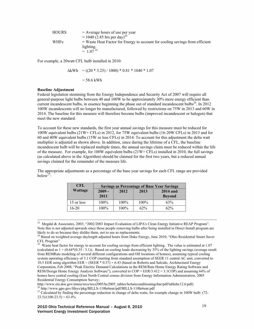
ISR = In Service Rate or percentage of units rebated that get installed.
= 0.868 HOURS = Average hours of use per year
= 1040 (2.85 hrs per day)9 WHFe = Waste Heat Factor for Energy to account for cooling savings from efficient
lighting. = 1.07 10
For example, a 20watt CFL bulb installed in 2010:
ΔkWh = ((20 * 3.25)/1000) * 0.86 * 1040 * 1.07 = 62.2 kWh Baseline Adjustment Federal legislation stemming from the Energy Independence and Security Act of 2007 will require all general-purpose light bulbs between 40 and 100W to be approximately 30% more energy efficient than current incandescent bulbs, in essence beginning the phase out of standard incandescent bulbs11. In 2012 100W incandescents will no longer be manufactured, followed by restrictions on 75W in 2013 and 60W in 2014. The baseline for this measure will therefore become bulbs (improved incandescent or halogen) that meet the new standard. To account for these new standards, the first year annual savings for this measure must be reduced for 100W equivalent bulbs (21W+ CFLs) in 2012, for 75W equivalent bulbs (16-20W CFLs) in 2013 and for 60 and 40W equivalent bulbs (15W or less CFLs) in 2014. To account for this adjustment the delta watt 7 Calculated by finding the new delta watts after incandescent bulb wattage reduced (from 100W to 72W in 2012, 75W to 53W in 2013 and 60W to 43W in 2014). 8 Starting with a first year ISR of 0.77 and a lifetime ISR of 0.97 from Nexus Market Research, RLW Analytics and GDS Associates study; “New England Residential Lighting Markdown Impact Evaluation, January 20, 2009”, and assuming 43% of the remaining 20% not installed in the first year replace incandescents (24 out of 56 respondents not purchased as spares; Nexus Market Research, RLW Analytics, October 2004; “Impact Evaluation of the Massachusetts, Rhode Island, and Vermont 2003 Residential Lighting Programs”, table 6-4). ISR is therefore calculated as 0.77 + (0.43*0.2) = 0.86. 9 Based on weighted average daylength adjusted hours from Duke Energy, June 2010; “Ohio Residential Smart Saver CFL Program” 10 Waste heat factor for energy to account for cooling savings from efficient lighting. The value is estimated at 1.07 (calculated as 1 + (0.64*(0.35 / 3.1)). Based on cooling loads decreasing by 35% of the lighting savings (average result from REMRate modeling of several different configurations and OH locations of homes), assuming typical cooling system operating efficiency of 3.1 COP (starting from standard assumption of SEER 11 central AC unit, converted to 10.5 EER using algorithm EER = (SEER * 0.37) + 6.43 (based on Roberts and Salcido, Architectural Energy Corporation, Feb 2008; “Peak Electric Demand Calculations in the REM/Rate Home Energy Rating Software and REM/Design Home Energy Analysis Software”), converted to COP = EER/3.412 = 3.1COP) and assuming 64% of homes have central cooling (East North Central census division from Energy Information Administration, 2005 Residential Energy Consumption Survey; http://www.eia.doe.gov/emeu/recs/recs2005/hc2005_tables/hc6airconditioningchar/pdf/tablehc12.6.pdf). 11 http://www.gpo.gov/fdsys/pkg/BILLS-110hr6enr/pdf/BILLS-110hr6enr.pdf

2010 Ohio Technical Reference Manual – August 6, 2010 14 Vermont Energy Investment Corporation
multiplier is adjusted as shown above. In addition, since during the lifetime of a CFL, the baseline incandescent bulb will be replaced multiple times, the annual savings claim must be reduced within the life of the measure. For example, for 100W equivalent bulbs (21W+ CFLs) installed in 2010, the full savings (as calculated above in the Algorithm) should be claimed for the first two years, but a reduced annual savings claimed for the remainder of the measure life. The appropriate adjustments as a percentage of the base year savings for each CFL range are provided below12:
Savings as Percentage of Base Year Savings CFL Wattage 2009 -
2011 2012 2013 2014 and
Beyond
15 or less 100% 100% 100% 63%
16-20 100% 100% 62% 62%
21W+ 100% 63% 63% 63%
Summer Coincident Peak Demand Savings
ΔkW = ((ΔWatts) /1000) * ISR * WHFd * CF
Where:
WHFd = Waste Heat Factor for Demand to account for cooling savings from efficient lighting = 1.21 13
CF = Summer Peak Coincidence Factor for measure = 0.11
For example, a 20watt CFL bulb installed in 2010:
ΔkW = ((20*3.25) / 1000) * 0.86 * 1.21 * 0.11 = 0.0074 kW Fossil Fuel Impact Descriptions and Calculation MMBTUWH = (((ΔWatts) /1000) * ISR * HOURS * 0.003413 * HF) / ηHeat Where:
MMBTUWH = gross customer annual heating MMBTU fuel increased usage for the measure from the reduction in lighting heat.
0.003413 = conversion from kWh to MMBTU HF = Heating Factor or percentage of light savings that must be heated
12 Calculated by finding the percentage reduction in change of delta watts, for example change in 100W bulb: (72-23.5)/(100-23.5) = 63.4% 13 Waste heat factor for demand to account for cooling savings from efficient lighting. The value is estimated at 1.21 (calculated as 1 + (0.64 / 3.1)). Based on typical cooling system operating efficiency of 3.1 COP (starting from standard assumption of SEER 11 central AC unit, converted to 10.5 EER using algorithm EER = (SEER * 0.37) + 6.43 (based on Roberts and Salcido, Architectural Energy Corporation, Feb 2008; “Peak Electric Demand Calculations in the REM/Rate Home Energy Rating Software and REM/Design Home Energy Analysis Software”), converted to COP = EER/3.412 = 3.1COP), and 64% of homes having central cooling (East North Central census division from Energy Information Administration, 2005 Residential Energy Consumption Survey).

2010 Ohio Technical Reference Manual – August 6, 2010 15 Vermont Energy Investment Corporation
= 0.4514 ηHeat = average heating system efficiency
= 0.72 15 For example, a 20watt CFL bulb installed in 2010: MMBTUWH = (((20 * 3.25)/1000) * 0.86 * 1040 * 0.003413 * 0.45) / 0.72 = 0.12 MMBtu Deemed O&M Cost Adjustment Calculation In order to account for the shift in baseline due to the Federal Legislation discussed above, the levelized baseline replacement cost over the lifetime of the CFL is calculated (see CFL baseline savings shift.xls). The key assumptions used in this calculation are documented below:
Standard Incandescent
Efficient Incandescent
Replacement Cost $0.50 $2.00 Component Life (years) (based on lamp life / assumed annual run hours)
116 317
The calculated net present value of the baseline replacement costs for CFL type and installation year are presented below:
NPV of baseline Replacement Costs CFL wattage 2010 2011 2012 2013 on
21W+ $4.48 $4.28 $4.28 $4.28 16-20W $3.57 $4.48 $4.28 $4.28 15W and less $3.81 $3.57 $4.48 $4.28
Version Date & Revision History Draft: Portfolio # Effective date: Date TRM will become effective End date: Date TRM will cease to be effective (or TBD) Referenced Documents: On the following page is an embedded Excel worksheet showing the calculation for the levelized annual replacement cost savings. Double click on the worksheet to open the file and review the calculations.
14 I.e. heating loads increase by 45% of the lighting savings (average result from REMRate modeling of several different configurations and OH locations of homes), 15 This has been estimated assuming that natural gas central furnace heating is typical for Ohio residences (65% of East North Central census division has a Natural Gas Furnace (based on Energy Information Administration, 2005 Residential Energy Consumption Survey: http://www.eia.doe.gov/emeu/recs/recs2005/hc2005_tables/hc4spaceheating/pdf/tablehc12.4.pdf)) In 2000, 40% of furnaces purchased in Ohio were condensing (based on data from GAMA, provided to Department of Energy during the federal standard setting process for residential heating equipment). Furnaces tend to last up to 20 years and so units purchased 10 years ago provide a reasonable proxy for the current mix of furnaces in the State. Assuming typical efficiencies for condensing and non condensing furnaces and duct losses, the average heating system efficiency is estimated as follows: (0.4*0.92) + (0.6*0.8) * (1-0.15) = 0.72 16 Assumes rated life of incandescent bulb of approximately 1000 hours. 17 VEIC best estimate of future technology.

2010 Ohio Technical Reference Manual – August 6, 2010 16 Vermont Energy Investment Corporation
Measure Life 9 Inc HalogenReal Discount Rate (RDR 5.00% 1 3
$0.50 $2.00
2010 Year 2010 2011 2012 2013 2014 2015 2016 2017 2018NPV
21W+ Baseline Replacement Costs $5.21 $0.00 $0.50 $2.00 $0.00 $0.00 $2.00 $0.00 $0.00 $2.00
16-20W Baseline Replacement Costs $4.15 $0.00 $0.50 $0.50 $2.00 $0.00 $0.00 $2.00 $0.00 $0.00
15W and less Baseline Replacement Costs $4.43 $0.00 $0.50 $0.50 $0.50 $2.00 $0.00 $0.00 $2.00 $0.00
2011 Year 2011 2012 2013 2014 2015 2016 2017 2018 2019NPV
21W+ Baseline Replacement Costs $4.97 $0.00 $2.00 $0.00 $0.00 $2.00 $0.00 $0.00 $2.00 $0.00
16-20W Baseline Replacement Costs $5.21 $0.00 $0.50 $2.00 $0.00 $0.00 $2.00 $0.00 $0.00 $2.00
15W and less Baseline Replacement Costs $4.15 $0.00 $0.50 $0.50 $2.00 $0.00 $0.00 $2.00 $0.00 $0.00
2012 Year 2012 2013 2014 2015 2016 2017 2018 2019 2020NPV
21W+ Baseline Replacement Costs $4.97 $0.00 $2.00 $0.00 $0.00 $2.00 $0.00 $0.00 $2.00 $0.00
16-20W Baseline Replacement Costs $4.97 $0.00 $2.00 $0.00 $0.00 $2.00 $0.00 $0.00 $2.00 $0.00
15W and less Baseline Replacement Costs $5.21 $0.00 $0.50 $2.00 $0.00 $0.00 $2.00 $0.00 $0.00 $2.00
2010 2011 2012 2013 on21W+ $5.21 $4.97 $4.97 $4.9716-20W $4.15 $5.21 $4.97 $4.9715W and less $4.43 $4.15 $5.21 $4.97
Multiply by 0.86 ISR2010 2011 2012 2013 on
21W+ $4.48 $4.28 $4.28 $4.2816-20W $3.57 $4.48 $4.28 $4.2815W and less $3.81 $3.57 $4.48 $4.28
CFL wattageNPV of baseline Replacement Costs
Calculation of O&M Impact for Baseline
CFL wattageNPV of baseline Replacement Costs
Bulb Assumptions
Component 1 Life (years)Component 1 Replacement Cost

2010 Ohio Technical Reference Manual – August 6, 2010 17 Vermont Energy Investment Corporation
Residential Direct Install - ENERGY STAR Compact Fluorescent Lamp (CFL) (Early Replacement) Official Measure Code (Measure Number: X-X-X-X (Existing Homes, Lighting End Use) Description A low wattage ENERGY STAR qualified compact fluorescent screw-in bulb is installed by an auditor, contractor or member of utility staff, in a residential location in place of an existing incandescent screw-in bulb through a Direct Install program. The characterization assumes protocols are implemented that guide installation of the bulb in to high use locations in the home. The CFL is provided at no cost to the end user. Definition of Efficient Equipment In order for this characterization to apply, the high-efficiency equipment must be an ENERGY STAR qualified compact fluorescent lamp. Definition of Baseline Equipment In order for this characterization to apply, the existing baseline equipment is assumed to be an incandescent light bulb. Deemed Calculation for this Measure
Annual kWh Savings = (CFLWatts * 3.25) * 0.901 Summer Coincident Peak kW Savings = (CFLWatts * 3.25) * 0.000108
Annual MMBtu Increase = (CFLWatts * 3.25) * 0.0018 Note: the delta watts multiplier of 3.25 will be adjusted in accordance with table presented below:
Delta Watts Multiplier18 CFL Wattage
2009 - 2011 2012 2013 2014 and Beyond
15 or less 3.25 3.25 3.25 2.05
16-20 3.25 3.25 2.00 2.00
21W+ 3.25 2.06 2.06 2.06
Adjustment to annual savings within life of measure:
Savings as Percentage of Base Year Savings CFL Wattage 2009 -
2011 2012 2013 2014 and
Beyond
15 or less 100% 100% 100% 63%
16-20 100% 100% 62% 62%
21W+ 100% 63% 63% 63%
Deemed Lifetime of Efficient Equipment The expected lifetime of the measure is 8 years19. 18 Calculated by finding the new delta watts after incandescent bulb wattage reduced (from 100W to 72W in 2012, 75W to 53W in 2013 and 60W to 43W in 2014). 19 Calculated using average rated life of compact fluorescent bulbs of 8000 hours (8000/1011 = 8 years), based on average for Energy Star CFLs (http://www.energystar.gov/index.cfm?c=cfls.pr_crit_cfls).

2010 Ohio Technical Reference Manual – August 6, 2010 18 Vermont Energy Investment Corporation
Deemed Measure Cost The full cost for this measure should be equal to the actual cost for implementation and installation (i.e. the cost of product and the labor for its installation). Deemed O&M Cost Adjustments The calculated levelized annual replacement cost savings for CFL type and installation year are presented below:
NPV of baseline Replacement Costs CFL wattage 2010 2011 2012 2013 on
21W+ $3.12 $4.03 $4.03 $4.03 16-20W $3.36 $3.12 $4.03 $4.03
15W and less $3.59 $3.36 $3.12 $4.03 Coincidence Factor The summer peak coincidence factor for this measure is 0.1120.
REFERENCE SECTION
Calculation of Savings Energy Savings
ΔkWh = ((ΔWatts) /1000) * ISR * HOURS * WHFe Where:
ΔWatts = Compact Fluorescent Watts * 3.2521 Note: The multiplier should be adjusted according to the table below to account for the change in
baseline stemming from the Energy Independence and Security Act of 2007 discussed below:
Delta Watts Multiplier22 CFL Wattage
2009 - 2011 2012 2013 2014 and Beyond
15 or less 3.25 3.25 3.25 2.05
16-20 3.25 3.25 2.00 2.00
21W+ 3.25 2.06 2.06 2.06
ISR = In Service Rate or percentage of units rebated that get installed.
= 0.81 23
Note, a provision in the Energy Independence and Security Act of 2007 requires that by January 1, 2020, all lamps meet efficiency criteria of at least 45 lumens per watt, in essence making the CFL baseline. Therefore after 2014 the measure life will have to be reduced each year to account for the number of years remaining to 2020. 20 Nexus Market Research, RLW Analytics and GDS Associates study; “New England Residential Lighting Markdown Impact Evaluation, January 20, 2009” 21 Average wattage of compact fluorescent from Duke Energy, June 2010; “Ohio Residential Smart Saver CFL Program” study was 15.47W, and the replacement incandescent bulb was 65.8W (note only data from responses who reported both wattage removed and wattage replaced are used). This is a ratio of 4.25 to 1, and so the delta watts is equal to the compact fluorescent bulb multiplied by 3.25. 22 Calculated by finding the new delta watts after incandescent bulb wattage reduced (from 100W to 72W in 2012, 75W to 53W in 2013 and 60W to 43W in 2014).
2010 Ohio Technical Reference Manual – August 6, 2010 19 Vermont Energy Investment Corporation
HOURS = Average hours of use per year = 1040 (2.85 hrs per day)24
WHFe = Waste Heat Factor for Energy to account for cooling savings from efficient lighting. = 1.07 25
For example, a 20watt CFL bulb installed in 2010:
ΔkWh = ((20 * 3.25) / 1000) * 0.81 * 1040 * 1.07 = 58.6 kWh Baseline Adjustment Federal legislation stemming from the Energy Independence and Security Act of 2007 will require all general-purpose light bulbs between 40 and 100W to be approximately 30% more energy efficient than current incandescent bulbs, in essence beginning the phase out of standard incandescent bulbs26. In 2012 100W incandescents will no longer be manufactured, followed by restrictions on 75W in 2013 and 60W in 2014. The baseline for this measure will therefore become bulbs (improved incandescent or halogen) that meet the new standard. To account for these new standards, the first year annual savings for this measure must be reduced for 100W equivalent bulbs (21W+ CFLs) in 2012, for 75W equivalent bulbs (16-20W CFLs) in 2013 and for 60 and 40W equivalent bulbs (15W or less CFLs) in 2014. To account for this adjustment the delta watt multiplier is adjusted as shown above. In addition, since during the lifetime of a CFL, the baseline incandescent bulb will be replaced multiple times, the annual savings claim must be reduced within the life of the measure. For example, for 100W equivalent bulbs (21W+ CFLs) installed in 2010, the full savings (as calculated above in the Algorithm) should be claimed for the first two years, but a reduced annual savings claimed for the remainder of the measure life. The appropriate adjustments as a percentage of the base year savings for each CFL range are provided below27:
Savings as Percentage of Base Year Savings CFL Wattage 2009 -
2011 2012 2013 2014 and
Beyond
15 or less 100% 100% 100% 63%
16-20 100% 100% 62% 62%
23 Megdal & Associates, 2003; “2002/2003 Impact Evaluation of LIPA's Clean Energy Initiative REAP Program”. Note this is not adjusted upwards since those people removing bulbs after being installed in Direct Install program are likely to do so because they dislike them, not to use as replacements. 24 Based on weighted average daylength adjusted hours from Duke Energy, June 2010; “Ohio Residential Smart Saver CFL Program” 25 Waste heat factor for energy to account for cooling savings from efficient lighting. The value is estimated at 1.07 (calculated as 1 + (0.64*(0.35 / 3.1)). Based on cooling loads decreasing by 35% of the lighting savings (average result from REMRate modeling of several different configurations and OH locations of homes), assuming typical cooling system operating efficiency of 3.1 COP (starting from standard assumption of SEER 11 central AC unit, converted to 10.5 EER using algorithm EER = (SEER * 0.37) + 6.43 (based on Roberts and Salcido, Architectural Energy Corporation, Feb 2008; “Peak Electric Demand Calculations in the REM/Rate Home Energy Rating Software and REM/Design Home Energy Analysis Software”), converted to COP = EER/3.412 = 3.1COP) and assuming 64% of homes have central cooling (East North Central census division from Energy Information Administration, 2005 Residential Energy Consumption Survey; http://www.eia.doe.gov/emeu/recs/recs2005/hc2005_tables/hc6airconditioningchar/pdf/tablehc12.6.pdf). 26 http://www.gpo.gov/fdsys/pkg/BILLS-110hr6enr/pdf/BILLS-110hr6enr.pdf 27 Calculated by finding the percentage reduction in change of delta watts, for example change in 100W bulb: (72-23.5)/(100-23.5) = 63.4%

2010 Ohio Technical Reference Manual – August 6, 2010 20 Vermont Energy Investment Corporation
Savings as Percentage of Base Year Savings CFL Wattage 2009 -
2011 2012 2013 2014 and
Beyond
21W+ 100% 63% 63% 63%
Summer Coincident Peak Demand Savings
ΔkW = ((ΔWatts) /1000) * ISR * WHFd * CF
Where:
WHFd = Waste Heat Factor for Demand to account for cooling savings from efficient lighting = 1.21 28
CF = Summer Peak Coincidence Factor for measure = 0.11
For example, a 20watt CFL bulb, installed in 2010:
ΔkW = ((20 * 3.25) / 1000) * 0.81 * 1.21 * 0.11 = 0.0070 kW Fossil Fuel Impact Descriptions and Calculation MMBTUWH = (((ΔWatts) /1000) * ISR * HOURS * 0.003413 * HF) / ηHeat Where:
MMBTUWH = gross customer annual heating MMBTU fuel increased usage for the measure from the reduction in lighting heat.
0.003413 = conversion from kWh to MMBTU HF = Heating Factor or percentage of light savings that must be heated = 0.4529 ηHeat = average heating system efficiency
= 0.72 30 For example, a 20watt CFL bulb, installed in 2010:
28 Waste heat factor for demand to account for cooling savings from efficient lighting. The value is estimated at 1.21 (calculated as 1 + (0.64 / 3.1)). Based on typical cooling system operating efficiency of 3.1 COP (starting from standard assumption of SEER 11 central AC unit, converted to 10.5 EER using algorithm EER = (SEER * 0.37) + 6.43 (based on Roberts and Salcido, Architectural Energy Corporation, Feb 2008; “Peak Electric Demand Calculations in the REM/Rate Home Energy Rating Software and REM/Design Home Energy Analysis Software”), converted to COP = EER/3.412 = 3.1COP), and 64% of homes having central cooling (East North Central census division from Energy Information Administration, 2005 Residential Energy Consumption Survey). 29 I.e. heating loads increase by 45% of the lighting savings (average result from REMRate modeling of several different configurations and OH locations of homes), 30 This has been estimated assuming that natural gas central furnace heating is typical for Ohio residences (65% of East North Central census division has a Natural Gas Furnace (based on Energy Information Administration, 2005 Residential Energy Consumption Survey: http://www.eia.doe.gov/emeu/recs/recs2005/hc2005_tables/hc4spaceheating/pdf/tablehc12.4.pdf)) In 2000, 40% of furnaces purchased in Ohio were condensing (based on data from GAMA, provided to Department of Energy during the federal standard setting process). Assuming typical efficiencies for condensing and non condensing furnace and duct losses, the average heating system efficiency is estimated as follows: (0.4*0.92) + (0.6*0.8) * (1-0.15) = 0.72

2010 Ohio Technical Reference Manual – August 6, 2010 21 Vermont Energy Investment Corporation
MMBTUWH = (((20 * 3.25)/1000) * 0.81 * 1040 * 0.003413 * 0.45) / 0.72 = 0.12 MMBtu Deemed O&M Cost Adjustment Calculation In order to account for the shift in baseline due to the Federal Legislation discussed above, the levelized baseline replacement cost over the lifetime of the CFL is calculated (see CFL baseline savings shift.xls). The key assumptions used in this calculation are documented below:
Standard Incandescent
Efficient Incandescent
Replacement Cost $0.50 $2.00 Component Life (years) (based on lamp life / assumed annual run hours)
131 332
The calculated net present value of the baseline replacement costs for CFL type and installation year are presented below:
NPV of baseline Replacement Costs CFL wattage 2010 2011 2012 2013 on
21W+ $3.12 $4.03 $4.03 $4.03 16-20W $3.36 $3.12 $4.03 $4.03
15W and less $3.59 $3.36 $3.12 $4.03 Version Date & Revision History Draft: Portfolio # Effective date: Date TRM will become effective End date: Date TRM will cease to be effective (or TBD) Referenced Documents: On the following page is an embedded Excel worksheet showing the calculation for the levelized annual replacement cost savings. Double click on the worksheet to open the file and review the calculations.
31 Assumes rated life of incandescent bulb of approximately 1000 hours. 32 VEIC best estimate of future technology.

2010 Ohio Technical Reference Manual – August 6, 2010 22 Vermont Energy Investment Corporation
Measure Life 8 Inc HalogenReal Discount Rate (RDR 5.00% 1 3
$0.50 $2.00
2010 Year 2010 2011 2012 2013 2014 2015 2016 2017NPV
21W+ Baseline Replacement Costs $3.86 $0.00 $0.50 $2.00 $0.00 $0.00 $2.00 $0.00 $0.00
16-20W Baseline Replacement Costs $4.15 $0.00 $0.50 $0.50 $2.00 $0.00 $0.00 $2.00 $0.00
15W and less Baseline Replacement Costs $4.43 $0.00 $0.50 $0.50 $0.50 $2.00 $0.00 $0.00 $2.00
2011 Year 2011 2012 2013 2014 2015 2016 2017 2018NPV
21W+ Baseline Replacement Costs $4.97 $0.00 $2.00 $0.00 $0.00 $2.00 $0.00 $0.00 $2.00
16-20W Baseline Replacement Costs $3.86 $0.00 $0.50 $2.00 $0.00 $0.00 $2.00 $0.00 $0.00
15W and less Baseline Replacement Costs $4.15 $0.00 $0.50 $0.50 $2.00 $0.00 $0.00 $2.00 $0.00
2012 Year 2012 2013 2014 2015 2016 2017 2018 2019NPV
21W+ Baseline Replacement Costs $4.97 $0.00 $2.00 $0.00 $0.00 $2.00 $0.00 $0.00 $2.00
16-20W Baseline Replacement Costs $4.97 $0.00 $2.00 $0.00 $0.00 $2.00 $0.00 $0.00 $2.00
15W and less Baseline Replacement Costs $3.86 $0.00 $0.50 $2.00 $0.00 $0.00 $2.00 $0.00 $0.00
2010 2011 2012 2013 on21W+ $3.86 $4.97 $4.97 $4.9716-20W $4.15 $3.86 $4.97 $4.9715W and less $4.43 $4.15 $3.86 $4.97
Multiply by 0.81 ISR2010 2011 2012 2013 on
21W+ $3.12 $4.03 $4.03 $4.0316-20W $3.36 $3.12 $4.03 $4.0315W and less $3.59 $3.36 $3.12 $4.03
CFL wattageNPV of baseline Replacement Costs
Bulb Assumptions
Component 1 Life (years)Component 1 Replacement Cost
CFL wattageNPV of baseline Replacement Costs
Calculation of O&M Impact for Baseline

2010 Ohio Technical Reference Manual – August 6, 2010 23 Vermont Energy Investment Corporation
Refrigerator and/or Freezer Retirement (Early Retirement) Official Measure Code (Measure Number: X-X-X-X (Program name, End Use) Description This measure involves the removal of an existing inefficient refrigerator or freezer from service, prior to its natural end of life (early retirement) 33. The program should target units with an age greater than 10 years, though it is expected that the average age will be greater than 20 years based on other similar program performance. Savings are calculated for the estimated energy consumption during the remaining life of the existing unit. Definition of Efficient Equipment n/a Definition of Baseline Equipment In order for this characterization to apply, the existing inefficient unit must be in working order and be removed from service. Deemed Savings for this Measure
Average Annual KWH Savings per
unit
Average Summer Coincident Peak kW
Savings per unit
Average Annual Fossil Fuel heating fuel increased usage
(MMBTU) per unit
Average Annual Water savings per
unit Refrigerator 1376 0.22 n/a n/a
Freezer 1244 0.20 n/a n/a Deemed Measure Life The remaining useful life of the retired unit is assumed to be 8 Years 34. Deemed Measure Cost The incremental cost for this measure will be the actual cost associated with the removal and recyling of the retired unit. Deemed O&M Cost Adjustments n/a Coincidence Factor A coincidence factor is not used to calculate peak demand savings for this measure. See discussion below.
REFERENCE SECTION
Calculation of Savings
33 This measure assumes a mix of primary and secondary units will be replaced (and the savings are reduced accordingly). By definition, the refrigerator in a household’s kitchen that satisfies the majority of the household’s demand for refrigeration is the primary refrigerator. One or more additional refrigerators in the household that satisfy supplemental needs for refrigeration are referred to as secondary refrigerators. 34 KEMA “Residential refrigerator recycling ninth year retention study”, 2004

2010 Ohio Technical Reference Manual – August 6, 2010 24 Vermont Energy Investment Corporation
Energy Savings ΔkWh = UECretired * ISAF
Where:
UECretired = Average in situ Unit Energy Consumption of retired unit, adjusted for part use Refrigerator = 1,619 kWh 35 Freezer = 1,464 kWh 36
ISAF = In Situ Adjustment Factor = 0.8537
Refrigerator ΔkWh = 1619 * 0.85
= 1376 kWh
Freezer ΔkWh = 1464 * 0.85 = 1244 kWh
Summer Coincident Peak Demand Savings ΔkW = (ΔkWh/8760) * TAF * LSAF
Where:
TAF = Temperature Adjustment Factor = 1.30 38
LSAF = Load Shape Adjustment Factor = 1.074 39
Refrigerator ΔkW = 1376/8760 * 1.30 * 1.074
= 0.22 kW
Freezer ΔkW = 1244/8760 * 1.30 * 1.074
= 0.20 kW
35 Based on regression-based savings estimates and incorporating the part-use factors, from Navigant Consulting, “AEP Ohio Energy Efficiency/Demand Response Plan Year 1 (1/1/2009-12/31/2009) Program Year Evaluation Report: Appliance Recycling Program”, March 9, 2010. 36 Ibid. 37 A recent California study suggests that in situ energy consumption of refrigerators is lower than the DOE test procedure would suggest (The Cadmus Group et al., “Residential Retrofit High Impact Measure Evaluation Report”, prepared for the California Public Utilities Commission, February 8, 2010). The magnitude of the difference – estimated as 6% lower for one California utility, 11% lower for a second, and 16% lower for a third – was a function of whether the recycled appliance was a primary or secondary unit, the size of the household and climate (warmer climates show a small difference between DOE test procedure estimated consumption and actual consumption; cooler climates had lower in situ consumption levels). Ideally, such an adjustment for Ohio should be computed using Ohio program participant data. However, such a calculation has not yet been performed for Ohio. In the absence of such a calculation, a 15% downward adjustment, which is near the high end of the range found in California, is assumed to be reasonable for Ohio given its cooler climate (relative to California). 38 Temperature adjustment factor based on Blasnik, Michael, "Measurement and Verification of Residential Refrigerator Energy Use, Final Report, 2003-2004 Metering Study", July 29, 2004 (p. 47). It assumes 64% of Ohio homes have central air conditioning. 39 Daily load shape adjustment factor also based on Blasnik, Michael, "Measurement and Verification of Residential Refrigerator Energy Use, Final Report, 2003-2004 Metering Study", July 29, 2004 (p. 48, using the average Existing Units Summer Profile for hours ending 16 through 18)
2010 Ohio Technical Reference Manual – August 6, 2010 25 Vermont Energy Investment Corporation
Fossil Fuel Impact Descriptions and Calculation n/a Water Impact Descriptions and Calculation n/a Deemed O&M Cost Adjustment Calculation n/a Version Date & Revision History Draft: Portfolio # Effective date: Date TRM will become effective End date: Date TRM will cease to be effective (or TBD)
2010 Ohio Technical Reference Manual – August 6, 2010 26 Vermont Energy Investment Corporation
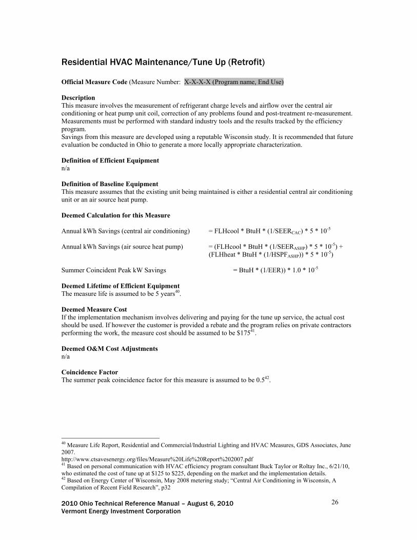
Residential HVAC Maintenance/Tune Up (Retrofit) Official Measure Code (Measure Number: X-X-X-X (Program name, End Use) Description This measure involves the measurement of refrigerant charge levels and airflow over the central air conditioning or heat pump unit coil, correction of any problems found and post-treatment re-measurement. Measurements must be performed with standard industry tools and the results tracked by the efficiency program. Savings from this measure are developed using a reputable Wisconsin study. It is recommended that future evaluation be conducted in Ohio to generate a more locally appropriate characterization. Definition of Efficient Equipment n/a Definition of Baseline Equipment This measure assumes that the existing unit being maintained is either a residential central air conditioning unit or an air source heat pump.
Deemed Calculation for this Measure Annual kWh Savings (central air conditioning) = FLHcool * BtuH * (1/SEERCAC) * 5 * 10-5 Annual kWh Savings (air source heat pump) = (FLHcool * BtuH * (1/SEERASHP) * 5 * 10-5) +
(FLHheat * BtuH * (1/HSPFASHP)) * 5 * 10-5) Summer Coincident Peak kW Savings = BtuH * (1/EER)) * 1.0 * 10-5 Deemed Lifetime of Efficient Equipment The measure life is assumed to be 5 years40. Deemed Measure Cost If the implementation mechanism involves delivering and paying for the tune up service, the actual cost should be used. If however the customer is provided a rebate and the program relies on private contractors performing the work, the measure cost should be assumed to be $17541. Deemed O&M Cost Adjustments n/a Coincidence Factor The summer peak coincidence factor for this measure is assumed to be 0.542.
40 Measure Life Report, Residential and Commercial/Industrial Lighting and HVAC Measures, GDS Associates, June 2007. http://www.ctsavesenergy.org/files/Measure%20Life%20Report%202007.pdf 41 Based on personal communication with HVAC efficiency program consultant Buck Taylor or Roltay Inc., 6/21/10, who estimated the cost of tune up at $125 to $225, depending on the market and the implementation details. 42 Based on Energy Center of Wisconsin, May 2008 metering study; “Central Air Conditioning in Wisconsin, A Compilation of Recent Field Research”, p32

2010 Ohio Technical Reference Manual – August 6, 2010 27 Vermont Energy Investment Corporation
REFERENCE SECTION
Calculation of Savings Energy Savings
ΔkWhCentral AC = (FLHcool * BtuH * (1/SEERCAC))/1000 * MFe ΔkWhAir Source Heat Pump = ((FLHcool * BtuH * (1/SEERASHP))/1000 * MFe)
+ (FLHheat * BtuH * (1/HSPFASHP))/1000 * MFe)
Where: FLHcool = Full load cooling hours Dependent on location as below:
Location Run Hours43 Akron 476
Cincinnati 664 Cleveland 426 Columbus 552
Dayton 631 Mansfield 474
Toledo 433 Youngstown 369
BtuH = Size of equipment in Btuh (note 1 ton = 12,000Btuh)
= Actual SEERCAC = SEER Efficiency of existing central air conditioning unit receiving
maintenence = Actual44
MFe = Maintenance energy savings factor = 0.0545 SEERASHP = SEER Efficiency of existing air source heat pump unit receiving maintenence
= Actual 46 FLHheat = Full load heating hours Dependent on location as below:
Location Run Hours47 Akron 1576
Cincinnati 1394 Cleveland 1567 Columbus 1272
Dayton 1438
43 Based on Full Load Hour assumptions taken from the ENERGY STAR calculator (http://www.energystar.gov/ia/business/bulk_purchasing/bpsavings_calc/Calc_CAC.xls) and reduced by 33% due to assumption that the average air conditioning is oversized by 50% (Neme, Proctor, Nadal, 1999; “National Energy Savings Potential From Addressing Residential HVAC Installation Problems”). Note this approach results in full load hour estimates within 10% of measured estimates from the Energy Center of Wisconsin, May 2008 study; “Central Air Conditioning in Wisconsin, A Compilation of Recent Field Research.” 44 Use actual SEER rating where it is possible to measure or reasonably estimate. When unknown use SEER 10 (VEIC estimate of existing unit efficiency, based on minimum federal standard between the years of 1992 and 2006) 45 Energy Center of Wisconsin, May 2008; “Central Air Conditioning in Wisconsin, A Compilation of Recent Field Research.” 46 Use actual SEER rating where it is possible to measure or reasonably estimate. When unknown use SEER 10 (VEIC estimate of existing unit efficiency, based on minimum federal standard between the years of 1992 and 2006) 47 Heating EFLH extracted from simulations conducted for Duke Energy, OH Joint Utility TRM, October 2009; “Technical Reference Manual (TRM) for Ohio Senate Bill 221Energy Efficiency and Conservation Program and 09-512-GE-UNC”

2010 Ohio Technical Reference Manual – August 6, 2010 28 Vermont Energy Investment Corporation
Location Run Hours47 Mansfield 1391
Toledo 1628 HSPFbase = Heating Season Performance Factor of existing air source heat pump unit
receiving maintenence = Actual48
For example, maintenance of a 3-ton, SEER 10 air conditioning unit in Cincinnati: ΔkWhCAC = (657 * 36000 * (1/10))/1000 * 0.05 = 118.3 kWh
For example, maintenance of a 3-ton, SEER 10, HSPF 6.8 air source heat pump unit in Cincinnati:
ΔkWhASHP = ((657 * 36000 * (1/10))/1000 * 0.05) + (1394 * 36000 * (1/6.8))/1000 * 0.05)
= 487.3 kWh
Summer Coincident Peak Demand Savings ΔkW = BtuH * (1/EER)/1000 * MFd * CF
Where: EER = EER Efficiency of existing unit receiving maintenence
= Calculate using Actual SEER = (SEER * 0.9)49
MFd = Maintenance demand savings factor = 0.0250 CF = Summer Peak Coincidence Factor for measure
= 0.551
For example, maintenance of 3-ton, SEER 10 (equals EER 9.0) unit: ΔkW = 36000 * (1/(9.0)/1000 * 0.02 * 0.5 = 0.04 kW
Fossil Fuel Impact Descriptions and Calculation n/a Water Impact Descriptions and Calculation n/a Deemed O&M Cost Adjustment Calculation Conservatively not included 48 Use actual HSPF rating where it is possible to measure or reasonably estimate. When unknown use HSPF 6.8 (Minimum Federal Standard between 1992 and 2006). 49 If SEER is unknown, default EER would be (10 * 0.9) = 9.0. Calculation based on prior VEIC assessment of industry equipment efficiency ratings. 50 Based on June 2010 personal conversation with Scott Pigg, author of Energy Center of Wisconsin, May 2008; “Central Air Conditioning in Wisconsin, A Compilation of Recent Field Research” suggesting the average WI unit system draw of 2.8kW under peak conditions, and average peak savings of 50W. 51 Based on Energy Center of Wisconsin, May 2008 metering study; “Central Air Conditioning in Wisconsin, A Compilation of Recent Field Research”, p32

2010 Ohio Technical Reference Manual – August 6, 2010 29 Vermont Energy Investment Corporation
Version Date & Revision History Draft: Portfolio # Effective date: Date TRM will become effective End date: Date TRM will cease to be effective (or TBD)

2010 Ohio Technical Reference Manual – August 6, 2010 30 Vermont Energy Investment Corporation
Central Air Conditioning (Time of Sale) Official Measure Code (Measure Number: X-X-X-X (Program name, End Use) Description This measure relates to the installation of a new Central Air Conditioning ducted split system meeting ENERGY STAR efficiency standards presented below. This measure could relate to the replacing of an existing unit at the end of its useful life, or the installation of a new system in an existing home (i.e. time of sale). Definition of Efficient Equipment In order for this characterization to apply, the efficient equipment is assumed to be a ducted split central air conditioning unit meeting the minimum ENERGY STAR efficiency level standards; 14.5 SEER and 12 EER. Definition of Baseline Equipment In order for this characterization to apply, the baseline equipment is assumed to be a ducted split central air conditioning unit meeting the Federal Standard efficiency level; 13 SEER and 11 EER. Deemed Calculation for this Measure
Annual kWh Savings = (Hours * BtuH * (1/13 - 1/SEERee))/1000 Summer Coincident Peak kW Savings = (BtuH * (1/11 - 1/EERee))/1000 * 0.5
Deemed Lifetime of Efficient Equipment The expected measure life is assumed to be 18 years 52. Deemed Measure Cost The incremental capital cost for this measure is provided below53.
Efficiency Level Cost per Ton SEER 14 $119
SEER 15 $238
SEER 16 $357
SEER 17 $476
SEER 18 $596
SEER 19 $715
SEER 20 $834
SEER 21 $908
Deemed O&M Cost Adjustments n/a Coincidence Factor The summer peak coincidence factor for this measure is assumed to be 0.554.
52 Measure Life Report, Residential and Commercial/Industrial Lighting and HVAC Measures, GDS Associates, June 2007. http://www.ctsavesenergy.org/files/Measure%20Life%20Report%202007.pdf 53 DEER 2008 Database Technology and Measure Cost Data (www.deeresources.com)
2010 Ohio Technical Reference Manual – August 6, 2010 31 Vermont Energy Investment Corporation
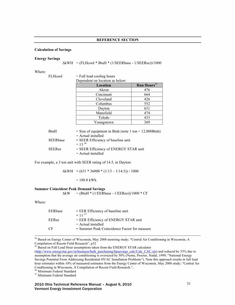
REFERENCE SECTION
Calculation of Savings Energy Savings
ΔkWH = (FLHcool * BtuH * (1/SEERbase - 1/SEERee))/1000
Where: FLHcool = Full load cooling hours Dependent on location as below:
Location Run Hours55 Akron 476
Cincinnati 664 Cleveland 426 Columbus 552
Dayton 631 Mansfield 474
Toledo 433 Youngstown 369
BtuH = Size of equipment in Btuh (note 1 ton = 12,000Btuh)
= Actual installed SEERbase = SEER Efficiency of baseline unit
= 13 56 SEERee = SEER Efficiency of ENERGY STAR unit
= Actual installed
For example, a 3 ton unit with SEER rating of 14.5, in Dayton:
ΔkWH = (631 * 36000 * (1/13 – 1/14.5)) / 1000
= 180.8 kWh Summer Coincident Peak Demand Savings
ΔkW = (BtuH * (1/EERbase - 1/EERee))/1000 * CF
Where:
EERbase = EER Efficiency of baseline unit = 11 57
EERee = EER Efficiency of ENERGY STAR unit = Actual installed
CF = Summer Peak Coincidence Factor for measure
54 Based on Energy Center of Wisconsin, May 2008 metering study; “Central Air Conditioning in Wisconsin, A Compilation of Recent Field Research”, p32 55 Based on Full Load Hour assumptions taken from the ENERGY STAR calculator (http://www.energystar.gov/ia/business/bulk_purchasing/bpsavings_calc/Calc_CAC.xls) and reduced by 33% due to assumption that the average air conditioning is oversized by 50% (Neme, Proctor, Nadal, 1999; “National Energy Savings Potential From Addressing Residential HVAC Installation Problems”). Note this approach results in full load hour estimates within 10% of measured estimates from the Energy Center of Wisconsin, May 2008 study; “Central Air Conditioning in Wisconsin, A Compilation of Recent Field Research.”.. 56 Minimum Federal Standard 57 Minimum Federal Standard

2010 Ohio Technical Reference Manual – August 6, 2010 32 Vermont Energy Investment Corporation
= 0.5 58
For example, a 3 ton unit with EER rating of 12:
ΔkW = (36000 * (1/11 – 1/12)) / 1000 * 0.5
= 0.14 kW Fossil Fuel Impact Descriptions and Calculation n/a Water Impact Descriptions and Calculation n/a Deemed O&M Cost Adjustment Calculation n/a Version Date & Revision History Draft: Portfolio # Effective date: Date TRM will become effective End date: Date TRM will cease to be effective (or TBD)
58 Based on Energy Center of Wisconsin, May 2008 metering study; “Central Air Conditioning in Wisconsin, A Compilation of Recent Field Research”, p32

2010 Ohio Technical Reference Manual – August 6, 2010 33 Vermont Energy Investment Corporation
Air Source Heat Pump (Time of Sale) Official Measure Code (Measure Number: X-X-X-X (Program name, End Use) Description This measure relates to the installation of a new Air Source Heat Pump system meeting ENERGY STAR efficiency standards presented below. This measure could relate to the replacing of an existing unit at the end of its useful life, or the installation of a new system in an existing home (i.e. time of sale). Definition of Efficient Equipment In order for this characterization to apply, the efficient equipment is assumed to be an Air Source Heat Pump unit meeting the minimum ENERGY STAR efficiency level standards; 14.5 SEER, 12 EER and 8.2 HSPF. Definition of Baseline Equipment In order for this characterization to apply, the baseline equipment is assumed to be an Air Source Heat Pump unit meeting the Federal Standard efficiency level; 13 SEER and 11 EER. Deemed Calculation for this Measure
Annual kWh Savings = (FLHcool * BtuH * (1/13 - 1/SEERee))/1000 + (FLHheat * BtuH * (1/7.7 – 1/HSPFee))/1000
Summer Coincident Peak kW Savings = (BtuH * (1/11 - 1/EERee))/1000 * 0.5
Deemed Lifetime of Efficient Equipment The expected measure life is assumed to be 18 years 59. Deemed Measure Cost The incremental capital cost for this measure is provided below60.
Efficiency Level Cost per Ton SEER 14 $137
SEER 15 $274
SEER 16 $411
SEER 17 $548
SEER 18 $685
Deemed O&M Cost Adjustments n/a Coincidence Factor The summer peak coincidence factor for this measure is assumed to be 0.561.
59 Measure Life Report, Residential and Commercial/Industrial Lighting and HVAC Measures, GDS Associates, June 2007. http://www.ctsavesenergy.org/files/Measure%20Life%20Report%202007.pdf 60 DEER 2008 Database Technology and Measure Cost Data (www.deeresources.com) 61 Based on Energy Center of Wisconsin, May 2008 metering study; “Central Air Conditioning in Wisconsin, A Compilation of Recent Field Research”, p32

2010 Ohio Technical Reference Manual – August 6, 2010 34 Vermont Energy Investment Corporation
REFERENCE SECTION
Calculation of Savings Energy Savings
ΔkWH = (FLHcool * BtuH * (1/SEERbase - 1/SEERee))/1000 + (FLHheat * BtuH * (1/HSPFbase – 1/HSPFee))/1000
Where: FLHcool = Full load cooling hours Dependent on location as below:
Location Run Hours62 Akron 476
Cincinnati 664 Cleveland 426 Columbus 552
Dayton 631 Mansfield 474
Toledo 433 Youngstown 369
BtuH = Size of equipment in Btuh (note 1 ton = 12,000Btuh)
= Actual installed SEERbase = SEER Efficiency of baseline unit
= 13 63 SEERee = SEER Efficiency of ENERGY STAR unit
= Actual installed FLHheat = Full load heating hours Dependent on location as below:
Location Run Hours64 Akron 1576
Cincinnati 1394 Cleveland 1567 Columbus 1272
Dayton 1438 Mansfield 1391
Toledo 1628 HSPFbase = Heating Season Performance Factor for baseline unit = 7.765
62 Based on Full Load Hour assumptions taken from the ENERGY STAR calculator (http://www.energystar.gov/ia/business/bulk_purchasing/bpsavings_calc/Calc_CAC.xls) and reduced by 33% due to assumption that the average air conditioning is oversized by 50% (Neme, Proctor, Nadal, 1999; “National Energy Savings Potential From Addressing Residential HVAC Installation Problems”). Note this approach results in full load hour estimates within 10% of measured estimates from the Energy Center of Wisconsin, May 2008 study; “Central Air Conditioning in Wisconsin, A Compilation of Recent Field Research.”. 63 Minimum Federal Standard; Federal Register, Vol. 66, No. 14, Monday, January 22, 2001/Rules and Regulations, p. 7170-7200. 64 Heating EFLH extracted from simulations conducted for Duke Energy, OH Joint Utility TRM, October 2009; “Technical Reference Manual (TRM) for Ohio Senate Bill 221Energy Efficiency and Conservation Program and 09-512-GE-UNC” 65 Minimum Federal Standard; Federal Register, Vol. 66, No. 14, Monday, January 22, 2001/Rules and Regulations, p. 7170-7200.

2010 Ohio Technical Reference Manual – August 6, 2010 35 Vermont Energy Investment Corporation
HSPFee = Heating Season Performance Factor for efficient unit = Actual Installed
For example, a 3 ton unit with SEER rating of 14.5 and HSPF of 8.2 in Dayton: ΔkWH = (631 * 36000 * (1/13 – 1/14.5)) / 1000 + (1438 * 36000 * (1/7.7 – 1/8.2)) / 1000
= 590.7 kWh
Summer Coincident Peak Demand Savings
ΔkW = BtuH * (1/EERbase - 1/EERee))/1000 * CF
Where: EERbase = EER Efficiency of baseline unit
= 11 66 EERee = EER Efficiency of ENERGY STAR unit
= Actual installed CF = Summer Peak Coincidence Factor for measure
= 0.5 67
For example, a 3 ton unit with EER rating of 12:
ΔkW = (36000 * (1/11 – 1/12)) / 1000 * 0.5
= 0.14 kW Fossil Fuel Impact Descriptions and Calculation n/a Water Impact Descriptions and Calculation n/a Deemed O&M Cost Adjustment Calculation n/a Version Date & Revision History Draft: Portfolio # Effective date: Date TRM will become effective End date: Date TRM will cease to be effective (or TBD)
66 Minimum Federal Standard 67 Based on Energy Center of Wisconsin, May 2008 metering study; “Central Air Conditioning in Wisconsin, A Compilation of Recent Field Research”, p32

2010 Ohio Technical Reference Manual – August 6, 2010 36 Vermont Energy Investment Corporation
Attic/Roof/Ceiling Insulation (Retrofit) Official Measure Code (Measure Number: X-X-X-X (Program name, End Use) Description This measure characterization is for the installation of new additional insulation in the attic/roof/ceiling of a residential building. The measure assumes that an auditor, contractor or utility staff member is on location, and will measure and record the existing and new insulation depth and type (to calculate R-values), the surface area of insulation added, and the efficiency of the heating system used in the home. Definition of Efficient Equipment The new insulation should meet any qualification criteria required for participation in the program. The new insulation R-value should include the total attic floor /roof assembly and include any existing insulation that is left in situ. Definition of Baseline Equipment The existing insulation R-value should include the total attic floor / roof assembly. An R-value of 5 should be assumed for the roof assembly plus the R-value of any existing insulation68. Deemed Calculation for this Measure Air conditioning Savings
Annual kWh Savings = ((1/Rexist – 1/Rnew) * CDH * 0.75 * Area) / 1000 / ηCool Summer Coincident Peak kW Savings = ΔkWh / FLHcool * 0.5 Space Heating Savings:
MMBTU Savings (fossil fuel heating) = ((1/Rexist – 1/Rnew) * HDD * 24 * Area) / 1,000,000 / ηHeat
Annual kWh Savings (electric heating)
= (((1/Rexist – 1/Rnew) * HDD * 24 * Area) / 1,000,000 / ηHeat) * 293.1
Deemed Lifetime of Efficient Equipment The measure life is assumed to be 25 years69. Deemed Measure Cost The actual insulation installation measure cost should be used. Deemed O&M Cost Adjustments n/a Coincidence Factor The summer peak coincidence factor for this measure is assumed to be 0.570.
68 The R-5 assumption for roof assembly is based on J.Neymark & Associates and National Renewable Energy Laboratory, June 2009; “BESTEST-EX Interim Test Procedure” p27. The attic floor and roof should be modeled as a system including solar gains and attic ventilation, and R-5 is the standard assumption for the thermal resistance of the whole attic/roof system. 69 Measure Life Report, Residential and Commercial/Industrial Lighting and HVAC Measures, GDS Associates, June 2007. http://www.ctsavesenergy.org/files/Measure%20Life%20Report%202007.pdf 70 Based on Energy Center of Wisconsin, May 2008 metering study; “Central Air Conditioning in Wisconsin, A Compilation of Recent Field Research”, p32

2010 Ohio Technical Reference Manual – August 6, 2010 37 Vermont Energy Investment Corporation
REFERENCE SECTION
Calculation of Savings Energy Savings
ΔkWh = ((1/Rexist – 1/Rnew) * CDH * DUA * Area) / 1000 / ηCool
Where: Rexist = existing effective whole-assembly thermal resistance value or R-value71 = actual recorded Rnew = new total effective whole-assembly thermal resistance value or R-value72 = actual recorded
CDH = Cooling Degree Hours73. Dependent on location:
Location Cooling Degree Hours (75°F set point)
Akron 3,986 Cincinnati 7,711 Cleveland 5,817 Columbus 4,367
Dayton 5,934 Toledo 4,401
Youngtown 3,689 DUA = Discretionary Use Adjustment to account for the fact that people do not
always operate their air conditioning system when the outside temperature is greater than 75°F
= 0.75 74 Area = Square footage of insulated area = actual recorded ηCool = Efficiency of Air Conditioning equipment = actual recorded
For example, insulating 1000 square feet of an attic floor from R-5 to R-30, in a Cincinnati home with AC SEER 10:
ΔkWh = ((1/Rexist – 1/Rnew) * CDH * DUA * Area) / 1000 / ηCool
= ((1/5 – 1/30) * 7711 * 0.75 * 1000) / 1000 / 10
= 96 kWh
Summer Coincident Peak Demand Savings ΔkW = ΔkWh / FLHcool *CF Where:
FLHcool = Full load cooling hours
71 If uninsulated assembly assume R-5. 72 Include the R-value for the assembly and any existing insulation remaining. 73 Derived by summing the delta between the average outdoor temperature and the base set point of 75 degrees (above which cooling is assumed to be used) each hour of the year. Hourly temperature data obtained from TMY3 data (http://rredc.nrel.gov/solar/) 74 Based on Energy Center of Wisconsin, May 2008 metering study; “Central Air Conditioning in Wisconsin, A Compilation of Recent Field Research”, p31

2010 Ohio Technical Reference Manual – August 6, 2010 38 Vermont Energy Investment Corporation
Dependent on location as below: Location Run Hours75
Akron 476 Cincinnati 664 Cleveland 426 Columbus 552
Dayton 631 Mansfield 474
Toledo 433 Youngstown 369
CF = Summer Peak Coincidence Factor for measure
= 0.5 76 For example, insulating 1000 square feet of an attic floor from R-5 to R-30, in a Cincinnati home with AC SEER 10: ΔkW = ΔkWh / FLHcool *CF = 129 / 657 * 0.5 = 0.1 kW Space Heating Savings Calculation
ΔMMBTU = ((1/Rexist – 1/Rnew) * HDD * 24 * Area) / 1,000,000 / ηHeat
Where: HDD = Heating Degree Days (60° base temperature) for location77
Location Heating Degree Days (60°F base temperature)
Akron 4,848 Cincinnati 3,853 Cleveland 4,626 Columbus 4,100
Dayton 4,430 Toledo 4,482
Youngtown 4,887
ηHeat = Average Net Heating System Efficiency (Equipment Efficiency * Distribution Efficiency) 78
75 Based on Full Load Hour assumptions taken from the ENERGY STAR calculator (http://www.energystar.gov/ia/business/bulk_purchasing/bpsavings_calc/Calc_CAC.xls) and reduced by 33% due to assumption that the average air conditioning is oversized by 50% (Neme, Proctor, Nadal, 1999; “National Energy Savings Potential From Addressing Residential HVAC Installation Problems”). Note this approach results in full load hour estimates within 10% of measured estimates from the Energy Center of Wisconsin, May 2008 study; “Central Air Conditioning in Wisconsin, A Compilation of Recent Field Research.” 76Based on Energy Center of Wisconsin, May 2008 metering study; “Central Air Conditioning in Wisconsin, A Compilation of Recent Field Research”, p32 77 The 10 year average annual heating degree day value, using a balance point for heating equipment use of 60 degrees was calculated for each location based on data obtained from http://www.engr.udayton.edu/weather/. The 60 degree balance point is used based on personal communication with Michael Blasnik, consultant to Columbia gas in May 2010, and derived from a billing analysis of approximately 600,000 Columbia Gas residential single family customers in Ohio. 78 The System Efficiency can be obtained either by recording the AFUE of the unit, or performing a steady state efficiency test. The Distribution Efficiency can be estimated via a visual inspection and by referring to a look up table

2010 Ohio Technical Reference Manual – August 6, 2010 39 Vermont Energy Investment Corporation
= actual recorded Note for homes with electric heat (resistance or heat pump), follow the MMBTU formula above and convert to kWh by multiplying by 293.1. For heat pumps the equipment efficiency used in the above algorithm should be the Coefficient Of Performance or COP (i.e., divide HSPF by 3.412; e.g., HSPF 7.7 is COP of 2.26). For example, insulating 1000 square feet of an attic floor from R-5 to R-30, in a Cincinnati home with a gas heating system with efficiency of 70%:
ΔMMBTU = ((1/Rexist – 1/Rnew) * HDD * 24 * Area) / 1,000,000 / ηHeat
= ((1/5 – 1/30) * 3,853 * 24 * 1,000) / 1,000,000 / 0.7 = 22 MMBtu
Water Impact Descriptions and Calculation n/a Deemed O&M Cost Adjustment Calculation n/a Version Date & Revision History Draft: Portfolio # Effective date: Date TRM will become effective End date: Date TRM will cease to be effective (or TBD)
such as that provided by the Building Performance Institute: (http://www.bpi.org/files/pdf/DistributionEfficiencyTable-BlueSheet.pdf) or by performing duct blaster testing. If there are more than one heating systems, the weighted (by consumption) average efficiency should be used. If the heating system or distribution is being upgraded within a package of measures together with the insulation upgrade, the new average heating system efficiency should be used.

2010 Ohio Technical Reference Manual – August 6, 2010 40 Vermont Energy Investment Corporation
ENERGY STAR Torchiere (Time of Sale) Official Measure Code (Measure Number: X-X-X-X (Program name, End Use) Description A high efficiency ENERGY STAR fluorescent torchiere is purchased in place of a baseline mix of halogen and incandescent torchieres and installed in a residential setting. Assumptions are based on a time of sale purchase, not as a retrofit or direct install installation. Definition of Efficient Equipment To qualify for this measure the fluorescent torchiere must meet ENERGY STAR efficiency standards. Definition of Baseline Equipment The baseline is based on a mix of halogen and incandescent torchieres. Deemed Savings for this Measure
Average Annual KWH Savings per
unit
Average Summer Coincident Peak kW
Savings per unit
Average Annual Fossil Fuel heating fuel savings (MMBTU) per unit
Average Annual Water savings per
unit Residential 128.9 0.015 - 0.257 n/a
Deemed Lifetime of Efficient Equipment The lifetime of the measure is assumed to be 8 years79. Deemed Measure Cost The incremental cost for this measure is assumed to be $5.0080. Deemed O&M Cost Adjustments The annual O&M Cost Adjustment savings is calculated as $2.52. Coincidence Factor The summer peak coincidence factor for this measure is 0.1181.
REFERENCE SECTION
Calculation of Savings Energy Savings
ΔkWH = ((ΔWattsTorch / 1000) * ISR * HOURS * WHFe
Where: ΔWattsTorch = Average delta watts per purchased ENERGY STAR torchiere
= 115.8 82
79 Measure Life Report, Residential and Commercial/Industrial Lighting and HVAC Measures, GDS Associates, June 2007. 80 DEER 2008 Database Technology and Measure Cost Data (www.deeresources.com) and consistent with Efficiency Vermont TRM. 81 Nexus Market Research, RLW Analytics and GDS Associates study; “New England Residential Lighting Markdown Impact Evaluation, January 20, 2009”

2010 Ohio Technical Reference Manual – August 6, 2010 41 Vermont Energy Investment Corporation
ISR = In Service Rate or percentage of units rebated that get installed. = 0.95 83
HOURS = Average hours of use per year = 1095 (3.0 hrs per day)84
WHFe = Waste Heat Factor for Energy to account for cooling savings from efficient lighting. = 1.07 85
ΔkWH = (115.8 /1000) * 0.95 * 1095 * 1.07 = 128.9 kWh
Summer Coincident Peak Demand Savings ΔkW = (Δ WattsTorch /1000) * ISR * WHFd * CF
Where:
WHFd = Waste Heat Factor for Demand to account for cooling savings from efficient lighting = 1.21 86
CF = Summer Peak Coincidence Factor for measure = 0.1187
ΔkW = (115.8 /1000) * 0.95 * 1.21 * 0.11 = 0.015 kW Fossil Fuel Impact Descriptions and Calculation MMBTUWH = ((ΔWattsTorch /1000) * ISR * HOURS * 0.003413 * HF) / ηHeat
82 Nexus Market Research, “Impact Evaluation of the Massachusetts, Rhode Island and Vermont 2003 Residential Lighting Programs”, Final Report, October 1, 2004, p. 43 (Table 4-9) 83 Nexus Market Research, RLW Analytics “Impact Evaluation of the Massachusetts, Rhode Island, and Vermont 2003 Residential Lighting Programs” table 6-3 on p63 indicates that 86% torchieres were installed and a further 9% were to be installed. Table6-7 on p67 shows that none are purchased as spares so we assume that all are installed in first year. (http://publicservice.vermont.gov/energy/ee_files/efficiency/eval/marivtreportfinal100104.pdf) 84 Nexus Market Research, “Impact Evaluation of the Massachusetts, Rhode Island and Vermont 2003 Residential Lighting Programs”, Final Report, October 1, 2004, p. 104 (Table 9-7) 85 Waste heat factor for energy to account for cooling savings from efficient lighting. The value is estimated at 1.07 (calculated as 1 + (0.64*(0.35 / 3.1)). Based on cooling loads decreasing by 35% of the lighting savings (average result from REMRate modeling of several different configurations and OH locations of homes), assuming typical cooling system operating efficiency of 3.1 COP (starting from standard assumption of SEER 11 central AC unit, converted to 10.5 EER using algorithm EER = (SEER * 0.37) + 6.43 (based on Roberts and Salcido, Architectural Energy Corporation, Feb 2008; “Peak Electric Demand Calculations in the REM/Rate Home Energy Rating Software and REM/Design Home Energy Analysis Software”), converted to COP = EER/3.412 = 3.1COP) and assuming 64% of homes have central cooling (East North Central census division from Energy Information Administration, 2005 Residential Energy Consumption Survey; http://www.eia.doe.gov/emeu/recs/recs2005/hc2005_tables/hc6airconditioningchar/pdf/tablehc12.6.pdf). 86 Waste heat factor for demand to account for cooling savings from efficient lighting. The value is estimated at 1.21 (calculated as 1 + (0.64 / 3.1)). Based on typical cooling system operating efficiency of 3.1 COP (starting from standard assumption of SEER 11 central AC unit, converted to 10.5 EER using algorithm EER = (SEER * 0.37) + 6.43 (based on Roberts and Salcido, Architectural Energy Corporation, Feb 2008; “Peak Electric Demand Calculations in the REM/Rate Home Energy Rating Software and REM/Design Home Energy Analysis Software”), converted to COP = EER/3.412 = 3.1COP), and 64% of homes having central cooling (East North Central census division from Energy Information Administration, 2005 Residential Energy Consumption Survey). 87 Nexus Market Research, RLW Analytics and GDS Associates study; “New England Residential Lighting Markdown Impact Evaluation, January 20, 2009”

2010 Ohio Technical Reference Manual – August 6, 2010 42 Vermont Energy Investment Corporation
Where:
MMBTUWH = gross customer annual heating MMBTU fuel increased usage for the measure from the reduction in lighting heat.
0.003413 = conversion from kWh to MMBTU HF = Heating Factor or percentage of light savings that must be heated = 0.4588 ηHeat = average heating system efficiency
= 0.72 89 MMBTUWH = ((115.8/1000) * 0.95 * 1095 * 0.003413 * 0.45) / 0.72 = 0.257 MMBtu Water Impact Descriptions and Calculation n/a Deemed O&M Cost Adjustment Calculation The annual O&M Cost Adjustment savings is calculated as $2.52, based on the following component costs and lifetimes90
Version Date & Revision History Draft: Portfolio # Effective date: Date TRM will become effective End date: Date TRM will cease to be effective (or TBD)
88 I.e. heating loads increase by 45% of the lighting savings (average result from REMRate modeling of several different configurations and OH locations of homes), 89 This has been estimated assuming that natural gas central furnace heating is typical for Ohio residences (65% of East North Central census division has a Natural Gas Furnace (based on Energy Information Administration, 2005 Residential Energy Consumption Survey: http://www.eia.doe.gov/emeu/recs/recs2005/hc2005_tables/hc4spaceheating/pdf/tablehc12.4.pdf)) In 2000, 40% of furnaces purchased in Ohio were condensing (based on data from GAMA, provided to Department of Energy during the federal standard setting process). Assuming typical efficiencies for condensing and non condensing furnace and duct losses, the average heating system efficiency is estimated as follows: (0.4*0.92) + (0.6*0.8) * (1-0.15) = 0.72 90 Cost data derived from Efficiency Vermont TRM. 91 Calculated using assumed average rated life of Energy Star compact fluorescent torchiere bulbs of 9710 hours (9710/1095= 8.87 years) (http://downloads.energystar.gov/bi/qplist/fixtures_prod_list.xls). 92 Based on VEIC assumption of baseline bulb (mix of incandescent and halogen) average rated life of 2000 hours.
Efficient Measure Baseline Measures Component Cost Life (yrs) Cost Life (yrs) Lamp $7.50 8.87 years91 $6.00 1.83 years92

2010 Ohio Technical Reference Manual – August 6, 2010 43 Vermont Energy Investment Corporation
Dedicated Pin Based Compact Fluorescent Lamp (CFL) Table Lamp (Time of Sale) Official Measure Code (Measure Number: X-X-X-X (Efficient Products, Lighting End Use) Description A dedicated pin based low wattage compact fluorescent (CFL) table lamp is purchased through a retail outlet in place of an equivalent incandescent bulb lamp. The incremental cost of the CFL lamp compared to an incandescent lamp is offset via either rebate coupons or via upstream markdowns. Assumptions are based on a time of sale purchase, not as a retrofit or direct install installation. This characterization assumes that the CFL is installed in a residential location. Definition of Efficient Equipment In order for this characterization to apply, the high-efficiency equipment must be dedicated pin based low wattage compact fluorescent (CFL) table lamp. Definition of Baseline Equipment The baseline equipment is an incandescent table lamp. Deemed Savings for this Measure
Average Annual KWH Savings per
unit
Average Summer Coincident Peak kW
Savings per unit
Average Annual Fossil Fuel heating fuel savings (MMBTU) per unit
Average Annual Water savings per
unit Residential 42.5 0.0061 - 0.085 n/a
Adjustment to annual savings within life of measure:
Savings as Percentage of Base Year Savings CFL Wattage 2009 -
2011 2012 2013 2014 and
Beyond
15 or less 100% 100% 100% 63%
16-20 100% 100% 62% 62%
21W+ 100% 63% 63% 63%
Deemed Lifetime of Efficient Equipment The expected lifetime of the measure is 8 years93. Deemed Measure Cost The incremental cost for this measure is assumed to be $894. Deemed O&M Cost Adjustments The calculated levelized annual replacement cost savings for CFL type and installation year are presented below: 93 Measure Life Report, Residential and Commercial/Industrial Lighting and HVAC Measures, GDS Associates, June 2007. http://www.ctsavesenergy.org/files/Measure%20Life%20Report%202007.pdf 94 Average table lamp measure in DEER 2008 Database Technology and Measure Cost Data (www.deeresources.com).

2010 Ohio Technical Reference Manual – August 6, 2010 44 Vermont Energy Investment Corporation
NPV of baseline Replacement Costs CFL wattage 2010 2011 2012 2013 on
21W+ $3.86 $4.97 $4.97 $4.97 16-20W $4.15 $3.86 $4.97 $4.97 15W and less $4.43 $4.15 $3.86 $4.97
Coincidence Factor The summer peak coincidence factor for this measure is 0.1195.
REFERENCE SECTION
Calculation of Savings Energy Savings
ΔkWh = ((ΔWatts) /1000) * ISR * HOURS * WHFe Where:
ΔWatts = Difference in wattage between CFL and incandescent bulb = 45.7 96
ISR = In Service Rate or percentage of units rebated that get installed. = 1.0 97
HOURS = Average hours of use per year = 869 98
WHFe = Waste Heat Factor for Energy to account for cooling savings from efficient lighting. = 1.07 99
ΔkWh = (45.7 / 1000) * 1.0 * 869 * 1.07
= 42.5 kWh Summer Coincident Peak Demand Savings
ΔkW = ((ΔWatts) /1000) * ISR * WHFd * CF
Where:
95 Nexus Market Research, RLW Analytics and GDS Associates study; “New England Residential Lighting Markdown Impact Evaluation, January 20, 2009” 96 Based on RLW Analytics, New England Residential Lighting Markdown Impact Evaluation, January 20, 2009. 97 VEIC is not aware of any evaluations that evaluate In Service Rates of table lamps, but feel it is appropriate to assume that those people purchasing a table lamp will install and use it. 98 Nexus Market Research, RLW Analytics and GDS Associates study; “New England Residential Lighting Markdown Impact Evaluation, January 20, 2009”, p50. 99 Waste heat factor for energy to account for cooling savings from efficient lighting. The value is estimated at 1.07 (calculated as 1 + (0.64*(0.35 / 3.1)). Based on cooling loads decreasing by 35% of the lighting savings (average result from REMRate modeling of several different configurations and OH locations of homes), assuming typical cooling system operating efficiency of 3.1 COP (starting from standard assumption of SEER 11 central AC unit, converted to 10.5 EER using algorithm EER = (SEER * 0.37) + 6.43 (based on Roberts and Salcido, Architectural Energy Corporation, Feb 2008; “Peak Electric Demand Calculations in the REM/Rate Home Energy Rating Software and REM/Design Home Energy Analysis Software”), converted to COP = EER/3.412 = 3.1COP) and assuming 64% of homes have central cooling (East North Central census division from Energy Information Administration, 2005 Residential Energy Consumption Survey; http://www.eia.doe.gov/emeu/recs/recs2005/hc2005_tables/hc6airconditioningchar/pdf/tablehc12.6.pdf).

2010 Ohio Technical Reference Manual – August 6, 2010 45 Vermont Energy Investment Corporation
WHFd = Waste Heat Factor for Demand to account for cooling savings from efficient lighting = 1.21 100
CF = Summer Peak Coincidence Factor for measure = 0.11
ΔkW = (45.7 / 1000) * 1.0 * 1.21 * 0.11
= 0.0061 kW Baseline Adjustment Federal legislation stemming from the Energy Independence and Security Act of 2007 will require all general-purpose light bulbs between 40 and 100W to be approximately 30% more energy efficient than current incandescent bulbs, in essence beginning the phase out of standard incandescent bulbs101. In 2012 100W incandescents will no longer be manufactured, followed by restrictions on 75W in 2013 and 60W in 2014. The baseline for this measure will therefore become bulbs (improved incandescent or halogen) that meet the new standard. To account for these new standards, the first year annual savings for this measure must be reduced for 100W equivalent bulbs (21W+ CFLs) in 2012, for 75W equivalent bulbs (16-20W CFLs) in 2013 and for 60 and 40W equivalent bulbs (15W or less CFLs) in 2014. To account for this adjustment the delta watt multiplier is adjusted as shown above. In addition, since during the lifetime of a CFL, the baseline incandescent bulb will be replaced multiple times, the annual savings claim must be reduced within the life of the measure. For example, for 100W equivalent bulbs (21W+ CFLs) installed in 2010, the full savings (as calculated above in the Algorithm) should be claimed for the first two years, but a reduced annual savings claimed for the remainder of the measure life. The appropriate adjustments as a percentage of the base year savings for each CFL range are provided below102:
Savings as Percentage of Base Year Savings CFL Wattage 2009 -
2011 2012 2013 2014 and
Beyond
15 or less 100% 100% 100% 63%
16-20 100% 100% 62% 62%
21W+ 100% 63% 63% 63%
Fossil Fuel Impact Descriptions and Calculation MMBTUWH = (((ΔWatts) /1000) * ISR * HOURS * 0.003413 * HF) / ηHeat Where:
MMBTUWH = gross customer annual heating MMBTU fuel increased usage for the measure from the reduction in lighting heat.
100 Waste heat factor for demand to account for cooling savings from efficient lighting. The value is estimated at 1.21 (calculated as 1 + (0.64 / 3.1)). Based on typical cooling system operating efficiency of 3.1 COP (starting from standard assumption of SEER 11 central AC unit, converted to 10.5 EER using algorithm EER = (SEER * 0.37) + 6.43 (based on Roberts and Salcido, Architectural Energy Corporation, Feb 2008; “Peak Electric Demand Calculations in the REM/Rate Home Energy Rating Software and REM/Design Home Energy Analysis Software”), converted to COP = EER/3.412 = 3.1COP), and 64% of homes having central cooling (East North Central census division from Energy Information Administration, 2005 Residential Energy Consumption Survey). 101 http://www.gpo.gov/fdsys/pkg/BILLS-110hr6enr/pdf/BILLS-110hr6enr.pdf 102 Calculated by finding the percentage reduction in change of delta watts, for example change in 100W bulb: (72-23.5)/(100-23.5) = 63.4%

2010 Ohio Technical Reference Manual – August 6, 2010 46 Vermont Energy Investment Corporation
0.003413 = conversion from kWh to MMBTU HF = Heating Factor or percentage of light savings that must be heated = 0.45103 ηHeat = average heating system efficiency
= 0.72 104 MMBTUWH = ((45.7 / 1000) * 1.0 * 869 * 0.003413 * 0.45) / 0.72 = 0.085 MMBtu Deemed O&M Cost Adjustment Calculation In order to account for the shift in baseline due to the Federal Legislation discussed above, the levelized baseline replacement cost over the lifetime of the CFL is calculated (see CFL Table Lamp baseline savings shift.xls). The key assumptions used in this calculation are documented below:
Standard Incandescent
Efficient Incandescent
Replacement Cost $0.50 $2.00 Component Life (years) (based on lamp life / assumed annual run hours)
1105 3106
The calculated net present value of the baseline replacement costs for CFL type and installation year are presented below:
NPV of baseline Replacement Costs CFL wattage 2010 2011 2012 2013 on
21W+ $3.86 $4.97 $4.97 $4.97 16-20W $4.15 $3.86 $4.97 $4.97 15W and less $4.43 $4.15 $3.86 $4.97
Version Date & Revision History Draft: Portfolio # Effective date: Date TRM will become effective End date: Date TRM will cease to be effective (or TBD) Referenced Documents: On the following page is an embedded Excel showing the calculation for the levelized annual replacement cost savings. Double click on the worksheet to open the file and review the calculations.
103 I.e. heating loads increase by 45% of the lighting savings (average result from REMRate modeling of several different configurations and OH locations of homes), 104 This has been estimated assuming that natural gas central furnace heating is typical for Ohio residences (65% of East North Central census division has a Natural Gas Furnace (based on Energy Information Administration, 2005 Residential Energy Consumption Survey: http://www.eia.doe.gov/emeu/recs/recs2005/hc2005_tables/hc4spaceheating/pdf/tablehc12.4.pdf)) In 2000, 40% of furnaces purchased in Ohio were condensing (based on data from GAMA, provided to Department of Energy during the federal standard setting process). Assuming typical efficiencies for condensing and non condensing furnace and duct losses, the average heating system efficiency is estimated as follows: (0.4*0.92) + (0.6*0.8) * (1-0.15) = 0.72 105 Assumes rated life of incandescent bulb of approximately 1000 hours. 106 VEIC best estimate of future technology.

2010 Ohio Technical Reference Manual – August 6, 2010 47 Vermont Energy Investment Corporation
Measure Life 8 Inc HalogenReal Discount Rate (RDR 5.00% 1 3
$0.50 $2.00
2010 Year 2010 2011 2012 2013 2014 2015 2016 2017NPV
21W+ Baseline Replacement Costs $3.86 $0.00 $0.50 $2.00 $0.00 $0.00 $2.00 $0.00 $0.00
16-20W Baseline Replacement Costs $4.15 $0.00 $0.50 $0.50 $2.00 $0.00 $0.00 $2.00 $0.00
15W and less Baseline Replacement Costs $4.43 $0.00 $0.50 $0.50 $0.50 $2.00 $0.00 $0.00 $2.00
2011 Year 2011 2012 2013 2014 2015 2016 2017 2018NPV
21W+ Baseline Replacement Costs $4.97 $0.00 $2.00 $0.00 $0.00 $2.00 $0.00 $0.00 $2.00
16-20W Baseline Replacement Costs $3.86 $0.00 $0.50 $2.00 $0.00 $0.00 $2.00 $0.00 $0.00
15W and less Baseline Replacement Costs $4.15 $0.00 $0.50 $0.50 $2.00 $0.00 $0.00 $2.00 $0.00
2012 Year 2012 2013 2014 2015 2016 2017 2018 2019NPV
21W+ Baseline Replacement Costs $4.97 $0.00 $2.00 $0.00 $0.00 $2.00 $0.00 $0.00 $2.00
16-20W Baseline Replacement Costs $4.97 $0.00 $2.00 $0.00 $0.00 $2.00 $0.00 $0.00 $2.00
15W and less Baseline Replacement Costs $3.86 $0.00 $0.50 $2.00 $0.00 $0.00 $2.00 $0.00 $0.00
2010 2011 2012 2013 on21W+ $3.86 $4.97 $4.97 $4.9716-20W $4.15 $3.86 $4.97 $4.9715W and less $4.43 $4.15 $3.86 $4.97
Bulb Assumptions
Component 1 Life (years)Component 1 Replacement Cost
CFL wattageNPV of baseline Replacement Costs
Calculation of O&M Impact for Baseline

2010 Ohio Technical Reference Manual – August 6, 2010 48 Vermont Energy Investment Corporation
Ceiling Fan with ENERGY STAR Light Fixture (Time of Sale) Official Measure Code (Measure Number: X-X-X-X (Program name, End Use) Description This measure describes the installation of an ENERGY STAR ceiling fan that uses a high efficiency motor and contains compact fluorescent bulbs in place of a standard fan with integral incandescent bulbs. Definition of Efficient Equipment The efficient equipment must be an ENERGY STAR certified ceiling fan with integral CFL bulbs. Definition of Baseline Equipment The baseline equipment is assumed to be a standard fan with integral incandescent bulbs. Deemed Savings for this Measure
Average Annual KWH Savings per
unit
Average Summer Coincident Peak kW
Savings per unit
Average Annual Fossil Fuel heating fuel savings (MMBTU) per unit
Average Annual Water savings per
unit 2010 -2013 167 0.019 - 0.33 n/a
2014 on 97 0.012 - 0.19 n/a Adjustment to annual savings within life of measure of 58% at 2014. Deemed Lifetime of Efficient Equipment The measure life is assumed to be 10 years107. Deemed Measure Cost The incremental cost for the ENERGY STAR ceiling fan is $86107. Deemed O&M Cost Adjustments The calculated net present value of the baseline replacement costs minus the CFL replacement cost for each installation year are presented below. Note this is per fan (i.e. 3 bulbs):
NPV of baseline Replacement Costs - CFL Replacement Costs
2010 2011 2012 2013 on $5.82 $8.85 $8.17 $7.45
Coincidence Factor The summer peak coincidence factor for this measure is 0.11108.
REFERENCE SECTION
Calculation of Savings
107 ENERGY STAR Ceiling Fan Savings Calculator (http://www.energystar.gov/ia/business/bulk_purchasing/bpsavings_calc/Ceiling_Fan_Savings_Calculator_Consumer.xls) 108 Nexus Market Research, RLW Analytics and GDS Associates study; “New England Residential Lighting Markdown Impact Evaluation, January 20, 2009”

2010 Ohio Technical Reference Manual – August 6, 2010 49 Vermont Energy Investment Corporation
Energy Savings ΔkWh = ((%low * (LowKWbase - LowKWee) + %med * (MedKWbase - MedKWee) + %high
* (HighKWbase - HighKWee)) * HOURSfan) + ((IncKW – CFLKW) * HOURSlight
* WHFe)
Where 109: %low = Percent of time on Low Speed = 40% %med = Percent of time on Medium Speed = 40%
%high = Percent of time on High Speed = 20% LowWattbase = Low speed baseline ceiling fan wattage = 0.0152kW LowWattee = Low speed ENERGY STAR ceiling fan wattage = 0.0117kW
MedWattbase = Medium speed baseline ceiling fan wattage = 0.0348kW
MedWattee = Medium speed ENERGY STAR ceiling fan wattage = 0.0314kW
HighWattbase = High speed baseline ceiling fan wattage = 0.0725kW
HighWattee = High speed ENERGY STAR ceiling fan wattage = 0.0715kW
HOURSfan = Typical fan operating hours (2.8/day110, 365 days per year) = 1022 hours
IncWatt = Incandescent bulb kW (assumes 3 * 60W bulb) = 0.180kW CFLWatt = CFL bulb kW (assumes 3 * 20W bulb) = 0.060kW HOURSlight = Typical lighting operating hours (3.5/day, 365 days per year)= 1277.5 hours
WHFe = Waste Heat Factor for Energy to account for cooling savings from efficient lighting. = 1.07 111
ΔkWh = ((0.4 * (0.0152 – 0.0117) + 0.4 * (0.0348 – 0.0314) + 0.2 * (0.0725 – 0.0715))
* 1022) + ((0.18 – 0.06) * 1277.5 * 1.07)
= 167 kWh
Baseline Adjustment Federal legislation stemming from the Energy Independence and Security Act of 2007 will require all general-purpose light bulbs between 40 and 100W to be approximately 30% more energy efficient than current incandescent bulbs, in essence beginning the phase out of standard incandescent bulbs. In 2012 100W incandescents will no longer be manufactured, followed by restrictions on 75W in 2013 and 60W in 2014. The baseline for this measure will therefore become bulbs (improved incandescent or halogen) that meet the new standard. To account for these new standards, first year annual savings for this measure must be reduced beginning in 2014. This measure assumes 60W baseline bulbs, which in 2014 will become 43W and so the annual savings beginning in 2014 should therefore be:
ΔkWh = ((0.4 * (0.0152 – 0.0117) + 0.4 * (0.0348 – 0.0314) + 0.2 * (0.0725 – 0.0715)) * 1022) + ((0.129 – 0.06) * 1277.5 * 1.07)
109 All data points (unless otherwise noted) come from the ENERGY STAR Ceiling Fan Savings Calculator (http://www.energystar.gov/ia/business/bulk_purchasing/bpsavings_calc/Ceiling_Fan_Savings_Calculator_Consumer.xls) 110 For East North Central location. 111 Waste heat factor for energy to account for cooling savings from efficient lighting. The value is estimated at 1.07 (calculated as 1 + (0.64*(0.35 / 3.1)). Based on cooling loads decreasing by 35% of the lighting savings (average result from REMRate modeling of several different configurations and OH locations of homes), assuming typical cooling system operating efficiency of 3.1 COP (starting from standard assumption of SEER 11 central AC unit, converted to 10.5 EER using algorithm EER = (SEER * 0.37) + 6.43 (based on Roberts and Salcido, Architectural Energy Corporation, Feb 2008; “Peak Electric Demand Calculations in the REM/Rate Home Energy Rating Software and REM/Design Home Energy Analysis Software”), converted to COP = EER/3.412 = 3.1COP) and assuming 64% of homes have central cooling (East North Central census division from Energy Information Administration, 2005 Residential Energy Consumption Survey; http://www.eia.doe.gov/emeu/recs/recs2005/hc2005_tables/hc6airconditioningchar/pdf/tablehc12.6.pdf).
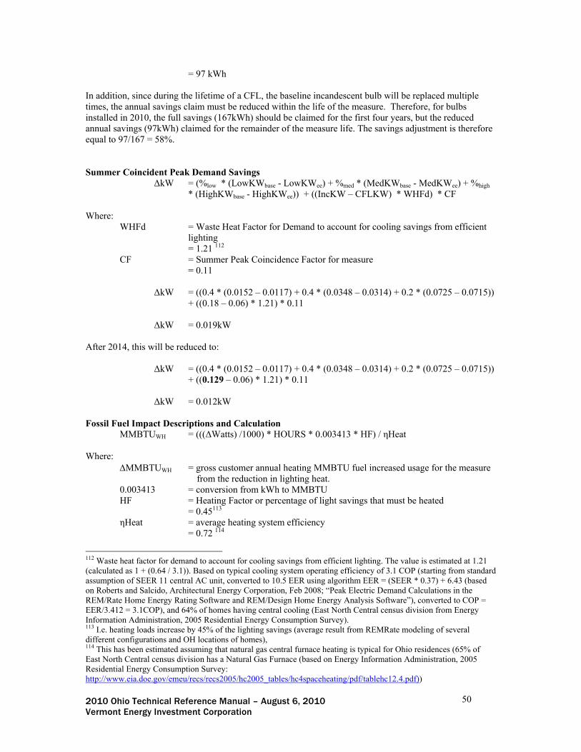
2010 Ohio Technical Reference Manual – August 6, 2010 50 Vermont Energy Investment Corporation
= 97 kWh In addition, since during the lifetime of a CFL, the baseline incandescent bulb will be replaced multiple times, the annual savings claim must be reduced within the life of the measure. Therefore, for bulbs installed in 2010, the full savings (167kWh) should be claimed for the first four years, but the reduced annual savings (97kWh) claimed for the remainder of the measure life. The savings adjustment is therefore equal to 97/167 = 58%. Summer Coincident Peak Demand Savings
ΔkW = (%low * (LowKWbase - LowKWee) + %med * (MedKWbase - MedKWee) + %high * (HighKWbase - HighKWee)) + ((IncKW – CFLKW) * WHFd) * CF
Where:
WHFd = Waste Heat Factor for Demand to account for cooling savings from efficient lighting = 1.21 112
CF = Summer Peak Coincidence Factor for measure = 0.11
ΔkW = ((0.4 * (0.0152 – 0.0117) + 0.4 * (0.0348 – 0.0314) + 0.2 * (0.0725 – 0.0715))
+ ((0.18 – 0.06) * 1.21) * 0.11
ΔkW = 0.019kW After 2014, this will be reduced to:
ΔkW = ((0.4 * (0.0152 – 0.0117) + 0.4 * (0.0348 – 0.0314) + 0.2 * (0.0725 – 0.0715)) + ((0.129 – 0.06) * 1.21) * 0.11
ΔkW = 0.012kW Fossil Fuel Impact Descriptions and Calculation MMBTUWH = (((ΔWatts) /1000) * HOURS * 0.003413 * HF) / ηHeat Where:
MMBTUWH = gross customer annual heating MMBTU fuel increased usage for the measure from the reduction in lighting heat.
0.003413 = conversion from kWh to MMBTU HF = Heating Factor or percentage of light savings that must be heated = 0.45113 ηHeat = average heating system efficiency
= 0.72 114
112 Waste heat factor for demand to account for cooling savings from efficient lighting. The value is estimated at 1.21 (calculated as 1 + (0.64 / 3.1)). Based on typical cooling system operating efficiency of 3.1 COP (starting from standard assumption of SEER 11 central AC unit, converted to 10.5 EER using algorithm EER = (SEER * 0.37) + 6.43 (based on Roberts and Salcido, Architectural Energy Corporation, Feb 2008; “Peak Electric Demand Calculations in the REM/Rate Home Energy Rating Software and REM/Design Home Energy Analysis Software”), converted to COP = EER/3.412 = 3.1COP), and 64% of homes having central cooling (East North Central census division from Energy Information Administration, 2005 Residential Energy Consumption Survey). 113 I.e. heating loads increase by 45% of the lighting savings (average result from REMRate modeling of several different configurations and OH locations of homes), 114 This has been estimated assuming that natural gas central furnace heating is typical for Ohio residences (65% of East North Central census division has a Natural Gas Furnace (based on Energy Information Administration, 2005 Residential Energy Consumption Survey: http://www.eia.doe.gov/emeu/recs/recs2005/hc2005_tables/hc4spaceheating/pdf/tablehc12.4.pdf))

2010 Ohio Technical Reference Manual – August 6, 2010 51 Vermont Energy Investment Corporation
MMBTUWH = (((120/1000) * 1277.5 * 0.003413 * 0.45) / 0.72 = 0.33 MMBtu
After 2014, this will be reduced to: MMBTUWH = (((69/1000) * 1277.5 * 0.003413 * 0.45) / 0.72 = 0.19 MMBtu
Water Impact Descriptions and Calculation n/a Deemed O&M Cost Adjustment Calculation In order to account for the shift in baseline due to the Federal Legislation discussed above, the levelized baseline replacement cost over the lifetime of the CFL is calculated (see CFL Ceiling Fan baseline savings shift.xls). The key assumptions used in this calculation are documented below:
Standard Incandescent
Efficient Incandescent
Replacement Cost $0.50 $2.00 Component Life (years) (based on lamp life / assumed annual run hours)
1115 3116
The calculated net present value of the baseline replacement costs minus the CFL replacement cost for each installation year are presented below. Note this is per fan (i.e. 3 bulbs):
NPV of baseline Replacement Costs - CFL Replacement Costs
2010 2011 2012 2013 on $5.82 $8.85 $8.17 $7.45
Version Date & Revision History Draft: Portfolio # Effective date: Date TRM will become effective End date: Date TRM will cease to be effective (or TBD) Referenced Documents: On the following page is an embedded Excel worksheet showing the calculation for the levelized annual replacement cost savings. Double click on the worksheet to open the file and review the calculations.
In 2000, 40% of furnaces purchased in Ohio were condensing (based on data from GAMA, provided to Department of Energy during the federal standard setting process for residential heating equipment). Furnaces tend to last up to 20 years and so units purchased 10 years ago provide a reasonable proxy for the current mix of furnaces in the State. Assuming typical efficiencies for condensing and non condensing furnaces and duct losses, the average heating system efficiency is estimated as follows: (0.4*0.92) + (0.6*0.8) * (1-0.15) = 0.72 115 Assumes rated life of incandescent bulb of approximately 1000 hours. 116 VEIC best estimate of future technology.
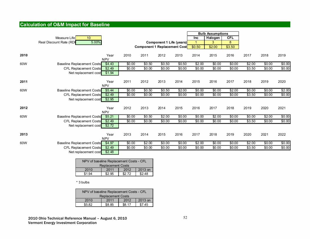
2010 Ohio Technical Reference Manual – August 6, 2010 52 Vermont Energy Investment Corporation
Measure Life 10 Inc Halogen CFLReal Discount Rate (RDR 5.00% 1 3 8
$0.50 $2.00 $3.50
2010 Year 2010 2011 2012 2013 2014 2015 2016 2017 2018 2019NPV
60W Baseline Replacement Costs $4.43 $0.00 $0.50 $0.50 $0.50 $2.00 $0.00 $0.00 $2.00 $0.00 $0.00CFL Replacement Costs $2.49 $0.00 $0.00 $0.00 $0.00 $0.00 $0.00 $0.00 $3.50 $0.00 $0.00
Net replacement cost $1.94
2011 Year 2011 2012 2013 2014 2015 2016 2017 2018 2019 2020NPV
60W Baseline Replacement Costs $5.44 $0.00 $0.50 $0.50 $2.00 $0.00 $0.00 $2.00 $0.00 $0.00 $2.00CFL Replacement Costs $2.49 $0.00 $0.00 $0.00 $0.00 $0.00 $0.00 $0.00 $3.50 $0.00 $0.00
Net replacement cost $2.95
2012 Year 2012 2013 2014 2015 2016 2017 2018 2019 2020 2021NPV
60W Baseline Replacement Costs $5.21 $0.00 $0.50 $2.00 $0.00 $0.00 $2.00 $0.00 $0.00 $2.00 $0.00CFL Replacement Costs $2.49 $0.00 $0.00 $0.00 $0.00 $0.00 $0.00 $0.00 $3.50 $0.00 $0.00
Net replacement cost $2.72
2013 Year 2013 2014 2015 2016 2017 2018 2019 2020 2021 2022NPV
60W Baseline Replacement Costs $4.97 $0.00 $2.00 $0.00 $0.00 $2.00 $0.00 $0.00 $2.00 $0.00 $0.00CFL Replacement Costs $2.49 $0.00 $0.00 $0.00 $0.00 $0.00 $0.00 $0.00 $3.50 $0.00 $0.00
Net replacement cost $2.48
2010 2011 2012 2013 on$1.94 $2.95 $2.72 $2.48
* 3 bulbs
2010 2011 2012 2013 on$5.82 $8.85 $8.17 $7.45
NPV of baseline Replacement Costs - CFL Replacement Costs
Bulb Assumptions
NPV of baseline Replacement Costs - CFL Replacement Costs
Calculation of O&M Impact for Baseline
Component 1 Life (years)Component 1 Replacement Cost

2010 Ohio Technical Reference Manual – August 6, 2010 53 Vermont Energy Investment Corporation
Efficient Refrigerator – ENERGY STAR and CEE TIER 2 (Time of Sale) Official Measure Code (Measure Number: X-X-X-X (Program name, End Use) Description
This measure relates to the purchase and installation of a new refrigerator meeting either ENERGY STAR or CEE TIER 2 specifications (defined as requiring >= 20% or >= 25% less energy consumption than an equivalent unit meeting federal standard requirements respectively). This is a time of sale measure characterization. Definition of Efficient Equipment
The efficient condition is a new refrigerator meeting either the ENERGY STAR or CEE TIER 2 efficiency standards. Definition of Baseline Equipment
The baseline condition is a new refrigerator meeting the minimum federal efficiency standard for refrigerator efficiency. Deemed Savings for this Measure
Efficiency Level
Refrigerator Configuration
Average Annual KWH Savings per
unit
Average Summer Coincident Peak kW
Savings per unit
Average Annual Fossil Fuel heating fuel savings
(MMBTU) per unit
Average Annual Water savings
per unit Bottom Freezer 119 0.021
Top Freezer 100 0.018 ENERGY
STAR Side by Side 142 0.025
n/a n/a
Bottom Freezer 149 0.026 Top Freezer 124 0.022
CEE TIER 2
Side by Side 177 0.031 n/a n/a
Deemed Lifetime of Efficient Equipment The measure life is assumed to be 17 Years 117. Deemed Measure Cost The incremental cost for this measure is assumed to be $30118 for an ENERGY STAR unit and $140119 for a CEE Tier 2 unit. Deemed O&M Cost Adjustments n/a Coincidence Factor A coincidence factor is not used to calculate peak demand savings for this measure. See discussion below.
117 Consistent with Efficiency Vermont and New Jersey TRMs 118 From ENERGY STAR calculator: http://www.energystar.gov/ia/business/bulk_purchasing/bpsavings_calc/Consumer_Residential_Refrig_Sav_Calc.xls 119 Based on weighted average of units participating in Efficiency Vermont program and retail cost data provided in Department of Energy, “TECHNICAL REPORT: Analysis of Amended Energy Conservation Standards for Residential Refrigerator-Freezers”, October 2005; http://www1.eere.energy.gov/buildings/appliance_standards/pdfs/refrigerator_report_1.pdf
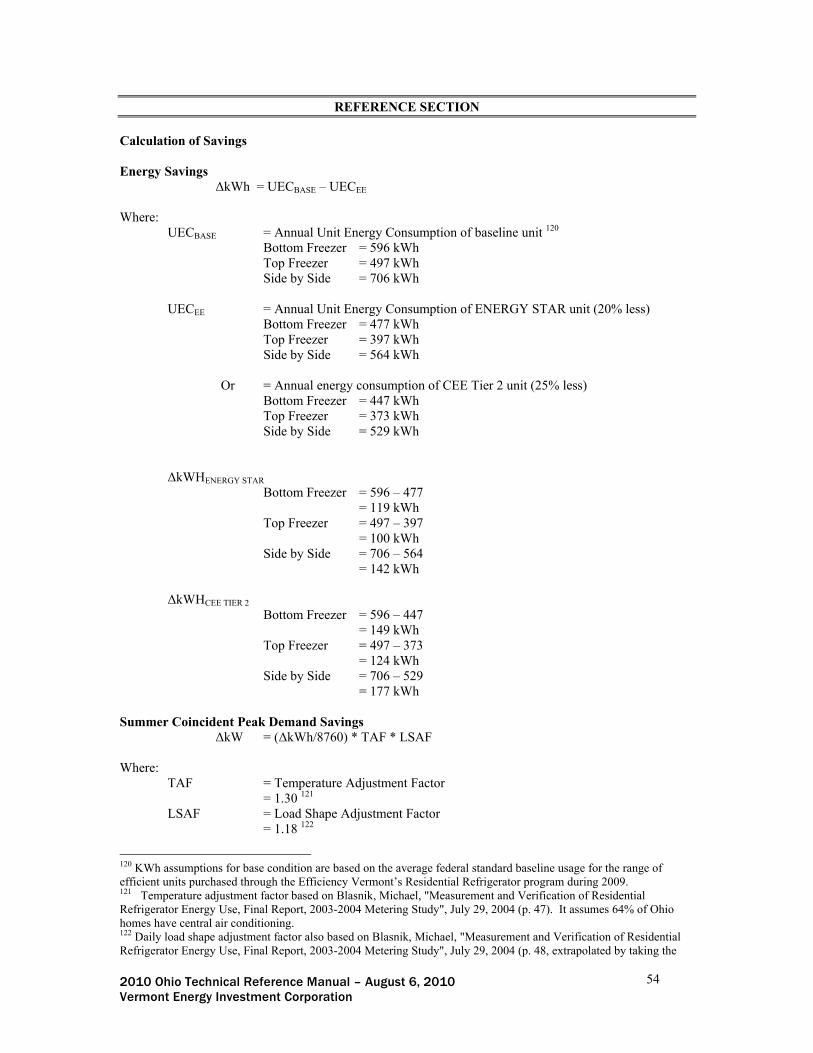
2010 Ohio Technical Reference Manual – August 6, 2010 54 Vermont Energy Investment Corporation
REFERENCE SECTION
Calculation of Savings Energy Savings
ΔkWh = UECBASE – UECEE
Where: UECBASE = Annual Unit Energy Consumption of baseline unit 120
Bottom Freezer = 596 kWh Top Freezer = 497 kWh Side by Side = 706 kWh
UECEE = Annual Unit Energy Consumption of ENERGY STAR unit (20% less) Bottom Freezer = 477 kWh Top Freezer = 397 kWh Side by Side = 564 kWh
Or = Annual energy consumption of CEE Tier 2 unit (25% less) Bottom Freezer = 447 kWh Top Freezer = 373 kWh Side by Side = 529 kWh
ΔkWHENERGY STAR
Bottom Freezer = 596 – 477 = 119 kWh
Top Freezer = 497 – 397 = 100 kWh
Side by Side = 706 – 564 = 142 kWh
ΔkWHCEE TIER 2
Bottom Freezer = 596 – 447 = 149 kWh
Top Freezer = 497 – 373 = 124 kWh
Side by Side = 706 – 529 = 177 kWh
Summer Coincident Peak Demand Savings
ΔkW = (ΔkWh/8760) * TAF * LSAF
Where: TAF = Temperature Adjustment Factor
= 1.30 121 LSAF = Load Shape Adjustment Factor
= 1.18 122
120 KWh assumptions for base condition are based on the average federal standard baseline usage for the range of efficient units purchased through the Efficiency Vermont’s Residential Refrigerator program during 2009. 121 Temperature adjustment factor based on Blasnik, Michael, "Measurement and Verification of Residential Refrigerator Energy Use, Final Report, 2003-2004 Metering Study", July 29, 2004 (p. 47). It assumes 64% of Ohio homes have central air conditioning. 122 Daily load shape adjustment factor also based on Blasnik, Michael, "Measurement and Verification of Residential Refrigerator Energy Use, Final Report, 2003-2004 Metering Study", July 29, 2004 (p. 48, extrapolated by taking the

2010 Ohio Technical Reference Manual – August 6, 2010 55 Vermont Energy Investment Corporation
ΔkWENERGY STAR
Bottom Freezer = 119/8760 * 1.3 * 1.18 = 0.021 kW
Top Freezer = 100/8760 * 1.3 * 1.18 = 0.018 kW
Side by Side = 142/8760 * 1.3 * 1.18 = 0.025 kW
ΔkWCEE TIER 2
Bottom Freezer = 149/8760 * 1.3 * 1.18 = 0.026 kW
Top Freezer = 124/8760 * 1.3 * 1.18 = 0.022 kW
Side by Side = 177/8760 * 1.3 * 1.18 = 0.031 kW
Fossil Fuel Impact Descriptions and Calculation n/a Water Impact Descriptions and Calculation n/a Deemed O&M Cost Adjustment Calculation n/a Version Date & Revision History Draft: Portfolio # Effective date: Date TRM will become effective End date: Date TRM will cease to be effective (or TBD)
ratio of existing summer to existing annual profile for hours ending 16 through 18, and multiplying by new annual profile).

2010 Ohio Technical Reference Manual – August 6, 2010 56 Vermont Energy Investment Corporation
Refrigerator Replacement (Low Income, Early Replacement) Official Measure Code (Measure Number: X-X-X-X (Program name, End Use) Description This measure describes the early removal of an existing inefficient refrigerator from service, prior to its natural end of life, and replacement with a new ENERGY STAR qualifying unit. This measure is suitable for a Low Income or Home Performance program. Savings are calculated for the estimated energy consumption during the remaining life of the existing unit. Definition of Efficient Equipment The efficient condition is a new replacement refrigerator meeting the ENERGY STAR efficiency standard (defined as requiring >= 20% less energy consumption than an equivalent unit meeting federal standard requirements). Definition of Baseline Equipment The baseline condition is the existing inefficient refrigerator for the remaining assumed useful life of the unit, and then for the remainder of the measure life the baseline becomes a new refrigerator meeting the minimum federal efficiency standard. Deemed Savings for this Measure
Average Annual KWH Savings per
unit
Average Summer Coincident Peak kW
Savings per unit
Average Annual Fossil Fuel heating fuel savings (MMBTU) per unit
Average Annual Water savings per
unit Remaining life of existing unit
(1st 8 years)
976 0.156 n/a n/a
Remaining measure life
(next 9 years)
100 0.018 n/a n/a
Deemed Lifetime of Efficient Equipment The measure life is assumed to be 17 Years 123. Deemed Lifetime of Replaced (Existing) Equipment (for early replacement measures only) The assumed remaining useful life of the existing refrigerator being replaced is 8 Years 124. Deemed Measure Cost The actual measure cost for removing the existing unit and installing the new should be used. Deemed O&M Cost Adjustments The net present value of the deferred replacement cost (the cost associated with the replacement of the existing unit with a standard unit that would have had to have occurred in 8 years, had the existing unit not been replaced) is calculated as $490.73125. Coincidence Factor A coincidence factor is not used to calculate peak demand savings for this measure. See discussion below.
123 Consistent with Efficiency Vermont and New Jersey TRMs 124 KEMA “Residential refrigerator recycling ninth year retention study”, 2004 125 Determined by calculating the Net Present Value (with a 5% discount rate) of the annuity payments from years 9 to 17 of a deferred replacement of a standard efficiency unit costing $1150 (from ENERGY STAR calculator: http://www.energystar.gov/ia/business/bulk_purchasing/bpsavings_calc/Consumer_Residential_Refrig_Sav_Calc.xls).
2010 Ohio Technical Reference Manual – August 6, 2010 57 Vermont Energy Investment Corporation
REFERENCE SECTION
Calculation of Savings Energy Savings
kWh for remaining life of existing unit (1st 8 years) = UECexisting – UECES
kWh for remaining measure life (next 9 years) = UECbase – UECES
Where: UECexisting = Unit Energy Consumption of existing refrigerator = 1,376 kWh 126 UECES = Unit Energy Consumption of new Energy Star refrigerator = 400 kWh 127
UECbase = Unit Energy Consumption of new baseline refrigerator
= 500 kWh 128 kWh for remaining life of existing unit (1st 8 years) = 1376 – 400 = 976 kWh kWh for remaining measure life (next 9 years) = 500 – 400 = 100 kWh
To incorporate this baseline shift, multiply annual savings by a Savings Adjustment of 10% after 8 years. Summer Coincident Peak Demand Savings
ΔkW = (ΔkWh/8760) * TAF * LSAF
Where: TAF = Temperature Adjustment Factor
= 1.30 129 LSAFexist = Load Shape Adjustment Factor for existing unit
= 1.074 130 LSAFnew = Load Shape Adjustment Factor for new unit
= 1.18 131
126 Based on regression-based savings estimates and incorporating the part-use factors, from Navigant Consulting, “AEP Ohio Energy Efficiency/Demand Response Plan Year 1 (1/1/2009-12/31/2009) Program Year Evaluation Report: Appliance Recycling Program”, March 9, 2010, and multiplied by in situ factor of 0.85 as discussed in Refrigetarot Retirement measure. 127 Approximate average consumption of typical ENERGY STAR refrigerator; http://www.energystar.gov/index.cfm?fuseaction=refrig.display_products_excel 128 Approximate average consumption of typical baseline refrigerator at federal standard efficiency levels; http://www.energystar.gov/index.cfm?fuseaction=refrig.display_products_excel 129 Temperature adjustment factor based on Blasnik, Michael, "Measurement and Verification of Residential Refrigerator Energy Use, Final Report, 2003-2004 Metering Study", July 29, 2004 (p. 47). It assumes 64% of Ohio homes have central air conditioning. 130 Daily load shape adjustment factor also based on Blasnik, Michael, "Measurement and Verification of Residential Refrigerator Energy Use, Final Report, 2003-2004 Metering Study", July 29, 2004 (p. 48, using the average Existing Units Summer Profile for hours ending 16 through 18) 131 Daily load shape adjustment factor also based on Blasnik, Michael, "Measurement and Verification of Residential Refrigerator Energy Use, Final Report, 2003-2004 Metering Study", July 29, 2004 (p. 48, extrapolated by taking the

2010 Ohio Technical Reference Manual – August 6, 2010 58 Vermont Energy Investment Corporation
ΔkW for remaining life of existing unit (1st 8 years) = (1376/8760 * 1.3 * 1.074) – (400/8760 * 1.3 * 1.18)
= 0.149 kW
ΔkW for remaining measure life (next 9 years) = 100/8760 * 1.3 * 1.18
= 0.018 kW Fossil Fuel Impact Descriptions and Calculation n/a Water Impact Descriptions and Calculation n/a Deemed O&M Cost Adjustment Calculation The net present value of the deferred replacement cost (the cost associated with the replacement of the existing unit with a standard unit that would have had to have occurred in 8 years, had the existing unit not been replaced) is calculated as $490.73132. Version Date & Revision History Draft: Portfolio # Effective date: Date TRM will become effective End date: Date TRM will cease to be effective (or TBD)
ratio of existing summer to existing annual profile for hours ending 16 through 18, and multiplying by new annual profile. 132 Determined by calculating the Net Present Value (with a 5% discount rate) of the annuity payments from years 9 to 17 of a deferred replacement of a standard efficiency unit costing $1150 (from ENERGY STAR calculator: http://www.energystar.gov/ia/business/bulk_purchasing/bpsavings_calc/Consumer_Residential_Refrig_Sav_Calc.xls).

2010 Ohio Technical Reference Manual – August 6, 2010 59 Vermont Energy Investment Corporation
Clothes Washer – ENERGY STAR and CEE TIER 3 (Time of Sale) Official Measure Code (Measure Number: X-X-X-X (Program name, End Use) Description This measure relates to the purchase (time of sale) and installation of a clothes washer exceeding either the ENERGY STAR or CEE TIER 3 minimum qualifying efficiency standards presented below:
Efficiency Level Modified Energy Factor (MEF) Water Factor (WF)
Federal Standard >= 1.26 No requirement ENERGY STAR (as of Jan 1, 2011)
>= 2.0 <= 6.0
CEE TIER 3 >= 2.20 <= 4.5
The modified energy factor (MEF) measures energy consumption of the total laundry cycle (washing and drying). It indicates how many cubic feet of laundry can be washed and dried with one kWh of electricity; the higher the number, the greater the efficiency. The Water Factor is the number of gallons needed for each cubic foot of laundry. A lower number indicates lower consumption and more efficient use of water. Definition of Efficient Equipment The efficient condition is a clothes washer meeting either the ENERGY STAR or CEE TIER 3 efficiency criteria presented above. Definition of Baseline Equipment The baseline condition is a clothes washer at the minimum federal baseline efficiency presented above. Deemed Savings for this Measure
Average Annual KWH Savings per
unit
Average Summer Coincident Peak kW
Savings per unit
Average Annual Fossil Fuel heating fuel savings (MMBTU) per unit
Average Annual Water savings (gal)
per unit ENERGY
STAR 202 0.028 0.447 (NGas), 0.02 (Oil),
0.013 (LP) 6,265
CEE TIER 3 233 0.033 0.516 (NGas), 0.023 (Oil), 0.015 (LP)
7,160
Deemed Lifetime of Efficient Equipment The measure life is assumed to be 11 years133. Deemed Measure Cost The incremental cost for this measure is assumed to be $258134 for an ENERGY STAR unit and $372 for a CEE TIER 3 unit135. Deemed O&M Cost Adjustments n/a
133 ENERGY STAR calculator (http://www.energystar.gov/index.cfm?fuseaction=find_a_product.showProductGroup&pgw_code=CW) 134 ENERGY STAR calculator (as above) 135 Based on an Efficiency Vermont market field study of incremental clothes washer cost between non-energy star and Tier 3 units, finding an average incremental cost to Tier 3 of $371.63.

2010 Ohio Technical Reference Manual – August 6, 2010 60 Vermont Energy Investment Corporation
Coincidence Factor The coincidence factor for this measure is assumed to be 0.045136.
REFERENCE SECTION
Calculation of Savings Energy Savings Savings are determined using Modified Energy Factor assumptions, applying the proportion of consumption used for water heating, clothes washer and clothes dryer operation and then to the mix of domestic hot water heating fuels and dryer fuels. Savings from reduced water usage are also factored in. For the full calculation see Clothes Washer Work Sheet, but the key assumptions and their sources are provided below:
Washer Volume = 3.23 cubic feet 137 Baseline MEF = 1.26 ENERGY STAR MEF = 2.0 CEE TIER 3 MEF = 2.2 Number of cycles per year = 320 138 % energy consumption for water heating, CW operation, Dryer operation = 26%, 7%, 67% 139 Water savings per load 140 ENERGY STAR = 19.6 gallons
CEE TIER 3 = 22.4 gallons Community/Municipal Water and Wastewater pump kWh savings per gallon water saved
= 0.0039kWh per gallon of water save141
Ohio DHW fuel mix142: Fuel % of Homes
Electric 27% Natural Gas 63%
Oil 6% Propane 4%
136 Calculated from Itron eShapes, which is 8760 hourly data by end use for Upstate New York and adjusted for OH peak definitions. 137 Average unit size from Efficiency Vermont program. 138 Weighted average of 2005 Residential Energy Consumption Survey (RECS) for East North Central Census Division: (http://www.eia.doe.gov/emeu/recs/recs2005/hc2005_tables/hc10homeappliaceindicators/pdf/tablehc12.10.pdf) 139 Based on the Clothes Washer Technical Support Document, Chapter 4, Engineering Analysis, Table 4.1, Page 4-5 http://www.eere.energy.gov/buildings/appliance_standards/residential/pdfs/chapter_4_engineering.pdf 140 Determined starting from gallons per load assumption from the ENERGY STAR calculator, dividing by water factor (gallons per cubic foot) to get cubic feet assumption and multiplying by each efficient case water factor. 141 Efficiency Vermont analysis of Community/Municipal Water and Wastewater pump energy consumption showed 0.0024 kWh pump energy consumption per gallon of water supplied, and 0.0015 kWh consumption per gallon for waste water treatment. 142 2005 Residential Energy Consumption Survey (RECS) for East North Central Census Division: (http://www.eia.doe.gov/emeu/recs/recs2005/hc2005_tables/hc8waterheating/pdf/tablehc12.8.pdf)

2010 Ohio Technical Reference Manual – August 6, 2010 61 Vermont Energy Investment Corporation
Ohio Dryer fuel mix143:
Fuel % of Homes Electric 66%
Natural Gas 34%
ΔkWHENERGY STAR = 202 kWh
ΔkWHCEE TIER 3 = 233 kWh
Summer Coincident Peak Demand Savings
ΔkW = ΔkWh/Hours * CF
Where:
Hours = Assumed Run hours of Clothes Washer = 320 144
CF = Summer Peak Coincidence Factor for measure = 0.033 145
ΔkWENERGY STAR = 202 / 320 * 0.045
= 0.028 kW
ΔkWCEE TIER 3 = 233 / 320 * 0.045
= 0.033 kW Fossil Fuel Impact Descriptions and Calculation For calculation see Clothes Washer Work Sheet. Savings are based on the mix of domestic hot water heating fuels and Dryer fuels. ENERGY STAR unit:
MMBtu Savings Natural Gas = 0.447 MMBtu MMBtu Savings Oil = 0.02 MMBtu MMBtu Savings Propane = 0.013 MMBtu
CEE TIER 3 unit:
MMBtu Savings Natural Gas = 0.516 MMBtu MMBtu Savings Oil = 0.023 MMBtu MMBtu Savings Propane = 0.015 MMBtu
Water Impact Descriptions and Calculation For calculation see Clothes Washer Work Sheet.
143 2005 Residential Energy Consumption Survey (RECS) for East North Central Census Division: (http://www.eia.doe.gov/emeu/recs/recs2005/hc2005_tables/hc9homeappliance/pdf/tablehc12.9.pdf) 144 Based on assumption of 1 hour average per cycle. # cycles based on weighted average of 2005 Residential Energy Consumption Survey (RECS) for East North Central Census Division (see CW Work Sheet). http://www.eia.doe.gov/emeu/recs/recs2005/hc2005_tables/hc10homeappliaceindicators/pdf/tablehc11.10.pdf 145 Calculated from Itron eShapes, which is 8760 hourly data by end use for Upstate New York and adjusted for OH peak definitions.

2010 Ohio Technical Reference Manual – August 6, 2010 62 Vermont Energy Investment Corporation
ENERGY STAR unit: Water Savings = 6,265 gallons CEE TIER 3 unit:
Water Savings = 7,160 gallons Deemed O&M Cost Adjustment Calculation n/a Reference Tables On the following page is the embedded Clothes Washer calculation spreadsheet. Double click on the window to open the Excel worksheet and follow the formulae. Version Date & Revision History Draft: Portfolio # Effective date: Date TRM will become effective End date: Date TRM will cease to be effective (or TBD) .

2010 Ohio Technical Reference Manual – August 6, 2010 63 Vermont Energy Investment Corporation
Clothes W asher W ork Sheet - EN ERG Y STAR and C EE TIER 31. Calculate kW h sav ing s per year p er mach in e:
kW h S avings pe r m ach ine = W as her Vo lum e* (1 /B aseM E F - 1 /E FF M EF ) * # C yclesE NERG Y S TA R 303 .2
C EE T IER 3 350 .1
W here : Source :W asher Vo lum e 3.23 Average o f E ffic iency V erm ont p rog ram
Base M EF 1.26 Federa l StandardE ST AR M EF 2 Energy Star m in im um standard (as o f Jan 1 2011)
CEE T IER 3 M EF 2.2 CEE T ie r 3 S tandard# Cycles 320 W eigh ted average o f 2005 Residen tia l E nergy Consum ption S urvey (RE CS) fo r E as t North Centra l Census D ivision
http ://www.eia .doe .gov/em eu/recs/rec s2005 /hc2005_tab les/hc10hom eappl iac eind ica to rs /pd f/tablehc12.10.pd f
2 . D iv id e saving s by end u se for w asher an d d ryer o peratio n:
E lectric ity Co n sum ptio n b y En d Use for W ash er/Dryer O peratio n
E lec tr ic it y C ons um ption
P erc ent by En d U s e Electr ic G as O il Electr ic G as O ilW a ter H ea tin g 2 6% 78 .8 0 .34 0 .34 91.0 0.39 0.39C W M ac hine Op eration 7% 21 .2 n /a n /a 24.5 n /a n/aD ry er 6 7% 203 .1 0 .69 n /a 234.6 0.80 n/aT o tal 100% 303 .2 350.1
3 . Calculate W ater Pu mp Saving sEN ERG Y
ST ARCEE TIE R
319 .6 22 .4 G a l Ca lcu la ted based on EN ERG Y S TA R ca lcu la to r (http ://www.energysta r.gov/ia /bus iness/bu lk_purc hasing /bps6265 7160 G a l Ca lcu la ted8 .4 9 .6 CCF Calcu la ted
24.4 27.9 kW h 0.0039kW h savings per ga llon saved - based on Effic iency Verm ont ana lysis o f com m un ity/m un icipa l wa ter a
4 . M u ltip ly sav ing s by DHW an d Dryer F uel M ix
O h io assu med D HW fuel m ix O h io assu med D ryer m ixENER G Y
S T AR CE E T IER 3
Electr ic 27% Electr ic 66% 202 .0 233.0Na tural G as 63% Natural G as 34% 0.447 0.516
O il 6% 0.020 0.023Propane 4% 0.013 0.015
("o ther" fuel ca tegory is s plit p roportionate ly be tween fue ls)h ttp ://ww w.e ia .doe.gov/em eu/recs/recs 2005/hc 2005_tab les/hc8waterheating /pdf/tab lehc 12 .8 .pdfh ttp ://ww w.e ia .doe.gov/em eu/recs/recs 2005/hc 2005_tab les/hc9hom eappl iance /pd f/tab lehc12.9 .pd f
D HW Fue l Mil lion hom es% o f
hom es Drye r F uelM illion hom es
% of hom es
E lectric 5 .1 27% E lec tr ic 9 .9 66%N atura l G as 11 .9 63% Natu ral G as 5 34%O il 1 .1 6% 14.9P ropane 0.7 4%
18.8
S ourc es :1 .w w w .eere. ene rg y.g ov/ bui ld ing s/ app lianc e_s tan dards /res id ential /c lw a sh _090 0_r.h tm l2 .C hap ter 4, E ngineer ing Ana ly s is , T a ble 4.1 , P age 4-5 w w w .e ere.en ergy .gov /bu ildings /ap pl ian ce _s tan da rd s/ re siden tia l/ pdfs /c ha pter_4 _eng in eerin g.pd f
kW h SavingsNatura l G as
O il
CEE T IE R 3E NERG Y S T AR
A nnua l W ater Savings/loadA nnua l G al lons saved
LP
A nnua l CCFW ater P um p S avings

2010 Ohio Technical Reference Manual – August 6, 2010 64 Vermont Energy Investment Corporation
Dehumidifier - ENERGY STAR (Time of Sale) Official Measure Code (Measure Number: X-X-X-X (Program name, End Use) Description A dehumidifier meeting the minimum qualifying efficiency standard established by ENERGY STAR on 10/1/2006 is purchased and installed in a residential setting in place of a unit that meets the minimum federal standard efficiency. Definition of Efficient Equipment To qualify for this measure, the new dehumidifier must meet the ENERGY STAR standards as of 10/1/2006 as defined below:
Capacity (pints/day)
ENERGY STAR Criteria (L/kWh)
≤25 ≥1.20 > 25 to ≤35 ≥1.40 > 35 to ≤45 ≥1.50 > 45 to ≤ 54 ≥1.60 > 54 to ≤ 75 ≥1.80
> 75 to ≤ 185 ≥2.50 Definition of Baseline Equipment The baseline for this measure is defined as a new dehumidifier that meets the Federal Standard efficiency standards as defined below:
Capacity (pints/day)
Federal Standard Criteria (L/kWh)
≤25 ≥1.10 > 25 to ≤35 ≥1.20 > 35 to ≤45 ≥1.20 > 45 to ≤ 54 ≥1.23 > 54 to ≤ 75 ≥1.55
> 75 to ≤ 185 ≥1.90 Deemed Savings for this Measure
Capacity Range (pints/day)
Average Annual KWH Savings per unit
Average Summer Coincident Peak kW
Savings per unit
Average Annual Fossil Fuel heating fuel savings (MMBTU) per unit
Average Annual Water savings per
unit ≤25 54 0.012
> 25 to ≤35 117 0.027 > 35 to ≤45 213 0.048 > 45 to ≤ 54 297 0.068 > 54 to ≤ 75 185 0.042
> 75 to ≤ 185 374 0.085
n/a n/a
2010 Ohio Technical Reference Manual – August 6, 2010 65 Vermont Energy Investment Corporation
Deemed Lifetime of Efficient Equipment The assumed lifetime of the measure is 12 years146 Deemed Measure Cost The assumed incremental capital cost for this measure is $45147
Deemed O&M Cost Adjustments n/a Coincidence Factor The coincidence factor is assumed to be 0.37 148
REFERENCE SECTION
Calculation of Savings Energy Savings
ΔkWH = (Av Capacity * 0.473) / 24 * Hours / L/kWh Where: 0.473 = Constant to convert Pints to Liters
Hours = Run hours per year = 1620 149 L/kWh = Liters of water per kWh consumed = As provided in tables above Annual kWh calculation results for each capacity class presented below:
Annual kWh
Capacity Range
Pints/day used
ENERGY STAR
Federal Standard
Savings
≤25 22.4 596 650 54
> 25 to ≤35 30 684 802 117
> 35 to ≤45 40 851 1064 213
> 45 to ≤ 54 49.5 988 1285 297
> 54 to ≤ 75 64.5 1144 1329 185
> 75 to ≤ 185 92.8 1185 1559 374 Summer Coincident Peak Demand Savings kW = kWh/Hours * CF Where:
CF = Summer Peak Coincidence Factor for measure = 0.37 150
146 ENERGY STAR Dehumidifier Calculator http://www.energystar.gov/ia/business/bulk_purchasing/bpsavings_calc/CalculatorConsumerDehumidifier.xls 147 Based on available data from the Department of Energy’s Life Cycle Cost analysis spreadsheet: http://www1.eere.energy.gov/buildings/appliance_standards/residential/docs/lcc_dehumidifier.xls 148 Assume usage is evenly distributed day vs night, weekend vs weekday and is used between April through the end of September (4392 possible hours). 1620 operating hours from ENERGY STAR Dehumidifier Calculator. Coincidence peak during summer peak is therefore 1620/4392 = 36.9% 149 ENERGY STAR Dehumidifier Calculator http://www.energystar.gov/ia/business/bulk_purchasing/bpsavings_calc/CalculatorConsumerDehumidifier.xls

2010 Ohio Technical Reference Manual – August 6, 2010 66 Vermont Energy Investment Corporation
Summer coincident peak demand calculation results for each capacity class presented below:
Annual kW
Capacity Range
Pints/day used
ENERGY STAR
Federal Standard
Savings
≤25 22.4 0.136 0.148 0.012 > 25 to ≤35 30 0.156 0.182 0.027 > 35 to ≤45 40 0.194 0.242 0.048 > 45 to ≤ 54 49.5 0.225 0.293 0.068 > 54 to ≤ 75 64.5 0.261 0.303 0.042 > 75 to ≤ 185 92.8 0.270 0.355 0.085
Fossil Fuel Impact Descriptions and Calculation n/a Water Impact Descriptions and Calculation n/a Deemed O&M Cost Adjustment Calculation n/a Version Date & Revision History Draft: Portfolio # Effective date: Date TRM will become effective End date: Date TRM will cease to be effective (or TBD)
150 Assume usage is evenly distributed day vs night, weekend vs weekday and is used between April through the end of September (4392 possible hours). 1620 operating hours from ENERGY STAR Dehumidifier Calculator. Coincidence peak during summer peak is therefore 1620/4392 = 36.9%

2010 Ohio Technical Reference Manual – August 6, 2010 67 Vermont Energy Investment Corporation
Room Air Conditioner - ENERGY STAR and CEE Tier 1 (Time of Sale) Official Measure Code (Measure Number: X-X-X-X (Program name, End Use) Description This measure relates to the purchase and installation of a room air conditioning unit that meets either the ENERGY STAR or CEE TIER 1 minimum qualifying efficiency specifications, in place of a baseline unit meeting minimum Federal Standard efficiency ratings presented below:
Product Class (BtuH) Federal Standard
(EER) ENERGY STAR
(EER) CEE TIER 1
(EER) 8,000 to 13,999 >= 9.8 >= 10.8 >= 11.3
Definition of Efficient Equipment To qualify for this measure the new room air conditioning unit must meet either the ENERGY STAR of CEE TIER 1 efficiency standards presented above. Definition of Baseline Equipment The baseline assumption is a new room air conditioning unit that meets the current minimum federal efficiency standards presented above. Deemed Savings for this Measure
Average Annual KWH Savings per unit
Average Summer Coincident Peak kW
Savings per unit
Average Annual Fossil Fuel heating fuel savings (MMBTU) per unit
Average Annual Water savings per
unit ENERGY
STAR 18.7 0.024 n/a n/a
CEE TIER 1 26.8 0.035 n/a n/a Deemed Lifetime of Efficient Equipment The measure life is assumed to be 12 years 151. Deemed Measure Cost The incremental cost for this measure is assumed to be $40 for an ENERGY STAR unit and $80 for a CEE TIER 1 unit 152. Deemed O&M Cost Adjustments n/a Coincidence Factor The coincidence factor for this measure is assumed to be 0.3153.
REFERENCE SECTION
Calculation of Savings
151 Measure Life Report, Residential and Commercial/Industrial Lighting and HVAC Measures, GDS Associates, June 2007. http://www.ctsavesenergy.org/files/Measure%20Life%20Report%202007.pdf 152 Based on field study conducted by Efficiency Vermont 153 Consistent with coincidence factors found in: RLW Report: Final Report Coincidence Factor Study Residential Room Air Conditioners, June 23, 2008 (http://www.puc.nh.gov/Electric/Monitoring%20and%20Evaluation%20Reports/National%20Grid/117_RLW_CF%20Res%20RAC.pdf)

2010 Ohio Technical Reference Manual – August 6, 2010 68 Vermont Energy Investment Corporation
Energy Savings ΔkWH = (Hours * BtuH * (1/EERbase - 1/EERee))/1000
Where:
Hours = Full Load Hours of room air conditioning unit = 233154
BtuH = Average size of rebated unit = 8500155
EERbase = Efficiency of baseline unit = 9.8156
EERee = Efficiency of ENERGY STAR unit = 10.8157
Or = Efficiency of CEE Tier 1 unit = 11.3158
ΔkWHENERGY STAR
= (233 * 8500 * (1/9.8 – 1/10.8)) / 1000 = 18.7 kWh
ΔkWHCEE TIER 1
= (233 * 8500 * (1/9.8 – 1/11.3)) / 1000 = 26.8 kWh
Summer Coincident Peak Demand Savings
ΔkW = BtuH * (1/EERbase - 1/EERee))/1000 * CF Where:
CF = Summer Peak Coincidence Factor for measure = 0.3159
ΔkWENERGY STAR
= (8500 * (1/9.8 – 1/10.8)) / 1000 * 0.3 = 0.024 kW
ΔkWCEE TIER 1
= (8500 * (1/9.8 – 1/11.3)) / 1000 * 0.3 = 0.035 kW
Fossil Fuel Impact Descriptions and Calculation n/a Water Impact Descriptions and Calculation n/a
154 The average ratio of FLH for Room AC (provided in RLW Report: Final Report Coincidence Factor Study Residential Room Air Conditioners, June 23, 2008: http://www.puc.nh.gov/Electric/Monitoring%20and%20Evaluation%20Reports/National%20Grid/117_RLW_CF%20Res%20RAC.pdf) to FLH for Central Cooling for the same location (provided by AHRI: http://www.energystar.gov/ia/business/bulk_purchasing/bpsavings_calc/Calc_CAC.xls) is 31%. This factor was applied to the FLH for Central Cooling provided for OH cities and averaged to come up with the assumption for FLH for Room AC. 155 Based on maximum capacity average from the RLW Report: Final Report Coincidence Factor Study Residential Room Air Conditioners, June 23, 2008. 156 Minimum Federal Standard for capacity range 157 Minimum qualifying standard for ENERGY STAR. 158 Minimum qualifying standard for CEE Tier 1. 159 Consistent with coincidence factors found in: RLW Report: Final Report Coincidence Factor Study Residential Room Air Conditioners, June 23, 2008 (http://www.puc.nh.gov/Electric/Monitoring%20and%20Evaluation%20Reports/National%20Grid/117_RLW_CF%20Res%20RAC.pdf)

2010 Ohio Technical Reference Manual – August 6, 2010 69 Vermont Energy Investment Corporation
Deemed O&M Cost Adjustment Calculation n/a Version Date & Revision History Draft: Portfolio # Effective date: Date TRM will become effective End date: Date TRM will cease to be effective (or TBD)
2010 Ohio Technical Reference Manual – August 6, 2010 70 Vermont Energy Investment Corporation
Room Air Conditioner Replacement - ENERGY STAR (Low Income, Early Replacement) Official Measure Code (Measure Number: X-X-X-X (Program name, End Use) Description This measure describes the early removal of an existing inefficient Room Air Conditioner unit from service, prior to its natural end of life, and replacement with a new ENERGY STAR qualifying unit. This measure is suitable for a Low Income or a Home Performance program. Savings are calculated between existing unit and efficient unit consumption during the remaining life of the existing unit, and between new baseline unit and efficient unit consumption for the remainder of the measure life. Definition of Efficient Equipment The efficient condition is a new replacement room air conditioning unit meeting the ENERGY STAR efficiency standard (i.e. with an efficiency rating greater than or equal to 10.8EER). Definition of Baseline Equipment The baseline condition is the existing inefficient room air conditioning unit for the remaining assumed useful life of the unit, and then for the remainder of the measure life the baseline becomes a new replacement unit meeting the minimum federal efficiency standard (i.e. with an efficiency rating greater than or equal to 9.8EER). Deemed Savings for this Measure
Average Annual KWH Savings per unit
Average Summer Coincident Peak kW
Savings per unit
Average Annual Fossil Fuel heating fuel savings (MMBTU) per unit
Average Annual Water savings per
unit Remaining
useful life of existing unit
(3 years)
73.8 0.095 n/a n/a
Remaining Measure Life (next 9 years)
18.7 0.024 n/a n/a
Deemed Lifetime of Efficient Equipment The measure life is assumed to be 12 Years160. Deemed Lifetime of Replaced (Existing) Equipment (for early replacement measures only) The assumed remaining useful life of the existing room air conditioning unit being replaced is 3 years161. Deemed Measure Cost The actual measure cost for removing the existing unit and installing the new should be used. Deemed O&M Cost Adjustments The net present value of the deferred replacement cost (the cost associated with the replacement of the existing unit with a standard unit that would have had to have occurred in 3 years, had the existing unit not been
160 Measure Life Report, Residential and Commercial/Industrial Lighting and HVAC Measures, GDS Associates, June 2007. http://www.ctsavesenergy.org/files/Measure%20Life%20Report%202007.pdf 161 Based on Connecticut TRM; Connecticut Energy Efficiency Fund; CL&P and UI Program Savings Documentation for 2008 Program Year

2010 Ohio Technical Reference Manual – August 6, 2010 71 Vermont Energy Investment Corporation
replaced) should be calculated as (Actual Cost of ENERGY STAR unit - $50 (incremental cost of ENERGY STAR unit over baseline unit162) * 69%163. Coincidence Factor The coincidence factor for this measure is assumed to be 0.3164.
REFERENCE SECTION
Calculation of Savings Energy Savings
kWh for remaining life of existing unit (1st 3 years) = (Hours * BtuH * (1/EERexist - 1/EERee))/1000
kWh for remaining measure life (next 9 years)
= (Hours * BtuH * (1/EERbase - 1/EERee))/1000
Where: Hours = Full Load Hours of room air conditioning unit
= 233165 BtuH = Average size of rebated unit
= 8500166 EERexist = Efficiency of existing unit
= 7.7167 EERbase = Efficiency of baseline unit
= 9.8168 EERee = Efficiency of ENERGY STAR unit
= 10.8169
kWh for remaining life of existing unit (1st 3 years) = (233 * 8500 * (1/7.7 – 1/10.8)) / 1000 = 73.8 kWh
kWh for remaining measure life (next 9 years)
= (233 * 8500 * (1/9.8 – 1/10.8)) / 1000
162 From ENERGY STAR calculator (ENERGY STAR - $220, Baseline - $170); http://www.energystar.gov/ia/business/bulk_purchasing/bpsavings_calc/CalculatorConsumerRoomAC.xls) 163 69% is the ratio of the Net Present Value (with a 5% discount rate) of the annuity payments from years 4 to 12 of a deferred replacement of a standard efficiency unit costing $170, divided by the standard efficiency unit cost ($170). The calculation is done in this way to allow the use of the known ENERGY STAR replacement cost to calculate an appropriate baseline replacement cost. 164 Consistent with coincidence factors found in: RLW Report: Final Report Coincidence Factor Study Residential Room Air Conditioners, June 23, 2008 (http://www.puc.nh.gov/Electric/Monitoring%20and%20Evaluation%20Reports/National%20Grid/117_RLW_CF%20Res%20RAC.pdf) 165 The average ratio of FLH for Room AC (provided in RLW Report: Final Report Coincidence Factor Study Residential Room Air Conditioners, June 23, 2008: http://www.puc.nh.gov/Electric/Monitoring%20and%20Evaluation%20Reports/National%20Grid/117_RLW_CF%20Res%20RAC.pdf) to FLH for Central Cooling for the same location (provided by AHRI: http://www.energystar.gov/ia/business/bulk_purchasing/bpsavings_calc/Calc_CAC.xls) is 31%. This factor was applied to the FLH for Central Cooling provided for OH cities and averaged to come up with the assumption for FLH for Room AC. 166 Based on maximum capacity average from the RLW Report; “Final Report Coincidence Factor Study Residential Room Air Conditioners, June 23, 2008.” 167 Based on Nexus Market Research Inc, RLW Analytics, December 2005; “Impact, Process, and Market Study of the Connecticut Appliance Retirement Program: Overall Report.” 168 Minimum Federal Standard for capacity range 169 Minimum qualifying standard for ENERGY STAR

2010 Ohio Technical Reference Manual – August 6, 2010 72 Vermont Energy Investment Corporation
= 18.7 kWh Summer Coincident Peak Demand Savings
kW for remaining life of existing unit (1st 3 years) = (BtuH * (1/EERexist - 1/EERee))/1000 * CF
kW for remaining measure life (next 9 years)
= (BtuH * (1/EERbase - 1/EERee))/1000 * CF
Where:
CF = Summer Peak Coincidence Factor for measure = 0.3170
kW for remaining life of existing unit (1st 3 years)
= (8500 * (1/7.7 – 1/10.8)) / 1000 * 0.3 = 0.095 kW
kW for remaining measure life (next 9 years)
= (8500 * (1/9.8 – 1/10.8)) / 1000 * 0.3 = 0.024 kW
Fossil Fuel Impact Descriptions and Calculation n/a Water Impact Descriptions and Calculation n/a Deemed O&M Cost Adjustment Calculation The net present value of the deferred replacement cost (the cost associated with the replacement of the existing unit with a standard unit that would have had to have occurred in 3 years, had the existing unit not been replaced) should be calculated as (Actual Cost of ENERGY STAR unit - $50 (incremental cost of ENERGY STAR unit over baseline unit171) * 69%172. Version Date & Revision History Draft: Portfolio # Effective date: Date TRM will become effective End date: Date TRM will cease to be effective (or TBD)
170 Consistent with coincidence factors found in: RLW Report: Final Report Coincidence Factor Study Residential Room Air Conditioners, June 23, 2008 (http://www.puc.nh.gov/Electric/Monitoring%20and%20Evaluation%20Reports/National%20Grid/117_RLW_CF%20Res%20RAC.pdf) 171 From ENERGY STAR calculator (ENERGY STAR - $220, Baseline - $170); http://www.energystar.gov/ia/business/bulk_purchasing/bpsavings_calc/CalculatorConsumerRoomAC.xls) 172 69% is the ratio of the Net Present Value (with a 5% discount rate) of the annuity payments from years 4 to 12 of a deferred replacement of a standard efficiency unit costing $170, divided by the standard efficiency unit cost ($170). The calculation is done in this way to allow the use of the known ENERGY STAR replacement cost to calculate an appropriate baseline replacement cost.

2010 Ohio Technical Reference Manual – August 6, 2010 73 Vermont Energy Investment Corporation
Room Air Conditioner Recycling (Early Retirement) Official Measure Code (Measure Number: X-X-X-X (Program name, End Use) Description This measure describes the savings resulting from running a drop off service taking existing inefficient Room Air Conditioner units from service, prior to their natural end of life. This measure assumes that a percentage of these units will be replaced with a baseline standard efficiency unit (note that if it is actually replaced by a new ENERGY STAR qualifying unit, the savings increment between baseline and ENERGY STAR will be recorded in the Efficient Products program). Definition of Efficient Equipment n/a. This measure relates to the retiring of an existing inefficient unit. Definition of Baseline Equipment The baseline condition is the existing inefficient room air conditioning unit. Deemed Savings for this Measure
Average Annual KWH Savings per unit
Average Summer Coincident Peak kW
Savings per unit
Average Annual Fossil Fuel heating fuel savings (MMBTU) per unit
Average Annual Water savings per
unit 103.6 0.906 n/a n/a
Deemed Lifetime of Replaced (Existing) Equipment (for early replacement measures only) The assumed remaining useful life of the existing room air conditioning unit being retired is 3 Years. Deemed Measure Cost The actual implementation cost for recycling the existing unit plus the cost for the replacement of some of the units of $129173. Deemed O&M Cost Adjustments The net present value of the deferred replacement cost (the cost associated with the replacement of those units that would be replaced, with a standard unit that would have had to have occurred in 3 years, had the existing unit not been replaced) is calculated as $89.36174. Coincidence Factor The coincidence factor for this measure is assumed to be 0.3175.
173 This is calculated by multiplying the percentage assumed to be replaced – 76% (from Based on Nexus Market Research Inc, RLW Analytics, December 2005; “Impact, Process, and Market Study of the Connecticut Appliance Retirement Program: Overall Report”) by the assumed cost of a standard efficiency unit of $170 (ENERGY STAR calculator; http://www.energystar.gov/ia/business/bulk_purchasing/bpsavings_calc/CalculatorConsumerRoomAC.xls). 0.76 * 170 = $129.2. 174 Determined by calculating the Net Present Value (with a 5% discount rate) of the annuity payments from years 4 to 12 of a deferred replacement of a standard efficiency unit costing $170 multiplied by the 76%, the percentage of units being replaced (i.e. 0.76 * $170 = $129.2. Baseline cost from ENERGY STAR calculator; http://www.energystar.gov/ia/business/bulk_purchasing/bpsavings_calc/CalculatorConsumerRoomAC.xls) 175 Consistent with coincidence factors found in: RLW Report: Final Report Coincidence Factor Study Residential Room Air Conditioners, June 23, 2008 (http://www.puc.nh.gov/Electric/Monitoring%20and%20Evaluation%20Reports/National%20Grid/117_RLW_CF%20Res%20RAC.pdf)

2010 Ohio Technical Reference Manual – August 6, 2010 74 Vermont Energy Investment Corporation
REFERENCE SECTION
Calculation of Savings Energy Savings
kWh = kWhexist – (%replaced * kWhnewbase)
= ((Hours * BtuH * (1/EERexist))/1000) - (%replaced * ((Hours * BtuH * (1/EERnewbase))/1000)
Where:
Hours = Full Load Hours of room air conditioning unit = 233176
BtuH = Average size of rebated unit = 8500177
EERexist = Efficiency of existing unit = 7.7178
%replaced = Percentage of units dropped off that are replaced = 76%179
EERbase = Efficiency of baseline unit = 9.8180
kWh = ((233 * 8500 * (1/7.7)) / 1000) – (0.76 * ((233 * 8500 * (1/9.8)) / 1000)
= 103.6 kWh
Summer Coincident Peak Demand Savings
kW = (kWexist – (%replaced * kWnewbase)) * CF
= ((BtuH * (1/EERexist))/1000) - (%replaced * ((BtuH * (1/EERnewbase))/1000) * CF
Where:
CF = Summer Peak Coincidence Factor for measure = 0.3181
176 The average ratio of FLH for Room AC (provided in RLW Report: Final Report Coincidence Factor Study Residential Room Air Conditioners, June 23, 2008: http://www.puc.nh.gov/Electric/Monitoring%20and%20Evaluation%20Reports/National%20Grid/117_RLW_CF%20Res%20RAC.pdf) to FLH for Central Cooling for the same location (provided by AHRI: http://www.energystar.gov/ia/business/bulk_purchasing/bpsavings_calc/Calc_CAC.xls) is 31%. This factor was applied to the FLH for Central Cooling provided for OH cities and averaged to come up with the assumption for FLH for Room AC. 177 Based on maximum capacity average from the RLW Report; “Final Report Coincidence Factor Study Residential Room Air Conditioners, June 23, 2008.” 178 Based on Nexus Market Research Inc, RLW Analytics, December 2005; “Impact, Process, and Market Study of the Connecticut Appliance Retirement Program: Overall Report.” 179 Based on Nexus Market Research Inc, RLW Analytics, December 2005; “Impact, Process, and Market Study of the Connecticut Appliance Retirement Program: Overall Report.” Report states that 63% were replaced with ENERGY STAR units and 13% with non-ENERGY STAR. However this formula assumes all are non-ENERGY STAR since the increment of savings between baseline units and ENERGY STAR would be recorded by the Efficient Products program when the new unit is purchased. 180 Minimum Federal Standard for capacity range 181 Consistent with coincidence factors found in: RLW Report: Final Report Coincidence Factor Study Residential Room Air Conditioners, June 23, 2008 (http://www.puc.nh.gov/Electric/Monitoring%20and%20Evaluation%20Reports/National%20Grid/117_RLW_CF%20Res%20RAC.pdf)

2010 Ohio Technical Reference Manual – August 6, 2010 75 Vermont Energy Investment Corporation
kW = ((8500 * (1/7.7)) / 1000) – (0.76 * ((8500 * (1/9.8)) / 1000) * 0.3
= 0.906 kW
Fossil Fuel Impact Descriptions and Calculation n/a Water Impact Descriptions and Calculation n/a Deemed O&M Cost Adjustment Calculation The net present value of the deferred replacement cost (the cost associated with the replacement of those units that would be replaced, with a standard unit that would have had to have occurred in 3 years, had the existing unit not been replaced) is calculated as $89.36182. Version Date & Revision History Draft: Portfolio # Effective date: Date TRM will become effective End date: Date TRM will cease to be effective (or TBD)
182 Determined by calculating the Net Present Value (with a 5% discount rate) of the annuity payments from years 4 to 12 of a deferred replacement of a standard efficiency unit costing multiplied by the 76%, the percentage of units being replaced (i.e. 0.76 * $170 = $129.2. Baseline cost from ENERGY STAR calculator; http://www.energystar.gov/ia/business/bulk_purchasing/bpsavings_calc/CalculatorConsumerRoomAC.xls)

2010 Ohio Technical Reference Manual – August 6, 2010 76 Vermont Energy Investment Corporation
Smart Strip Power Strip (Time of Sale) Official Measure Code (Measure Number: X-X-X-X (Program name, End Use) Description This measure relates to Controlled Power Strips (or Smart Strips) which are multi-plug power strips with the ability to automatically disconnect specific connected loads depending upon the power draw of a control load, also plugged into the strip. Power is disconnected from the switched (controlled) outlets when the control load power draw is reduced below a certain adjustable threshold, thus turning off the appliances plugged into the switched outlets. By disconnecting, the standby load of the controlled devices, the overall load of a centralized group of equipment (i.e. entertainment centers and home office) can be reduced. Uncontrolled outlets are also provided that are not affected by the control device and so are always providing power to any device plugged into it. This measure characterization provides savings for a 5-plug strip and a 7-plug strip. Definition of Efficient Equipment The efficient case is the use of a 5 or 7-plug smart strip. Definition of Baseline Equipment The assumed baseline is a standard power strip that does not control connected loads. Deemed Savings for this Measure
Average Annual KWH Savings per unit
Average Summer Coincident Peak kW
Savings per unit
Average Annual Fossil Fuel heating fuel savings (MMBTU) per unit
Average Annual Water savings per
unit 5- Plug 56.5 0.0063 n/a n/a 7- Plug 102.8 0.012 n/a n/a Deemed Lifetime of Efficient Equipment The assumed lifetime of the smart strip is 4 years183. Deemed Measure Cost The incremental cost of a smart strip over a standard power strip with surge protection is assumed to be $16 for a 5-plug and $26 for a 7-plug184. Deemed O&M Cost Adjustments n/a Coincidence Factor The summer peak coincidence factor for this measure is assumed to be 0.8185.
REFERENCE SECTION
Calculation of Savings
183 David Rogers, Power Smart Engineering, October 2008; “Smart Strip electrical savings and usability”, p22. 184 Price survey performed in NYSERDA Measure Characterization for Advanced Power Strips, p4 185 Efficiency Vermont coincidence factor for smart strip measure –in the absence of empirical evaluation data, this was based on assumptions of the typical run pattern for televisions and computers in homes.

2010 Ohio Technical Reference Manual – August 6, 2010 77 Vermont Energy Investment Corporation
Energy Savings 186
ΔkWh5-Plug = 56.5 kWh ΔkWh7-Plug = 102.8 kWh
Summer Coincident Peak Demand Savings kW = kWh / Hours * CF Where:
Hours = Annual number of hours during which the controlled standby loads are turned off by the Smart Strip.
= 7,129187 CF = Summer Peak Coincidence Factor for measure = 0.8188
ΔkW5-Plug = 56.5 / 7129 * 0.8 = 0.0063 kW ΔkW7-Plug = 102.8 / 7129 * 0.8 = 0.012 kW
Fossil Fuel Impact Descriptions and Calculation n/a Water Impact Descriptions and Calculation n/a Deemed O&M Cost Adjustment Calculation n/a Version Date & Revision History Draft: Portfolio # Effective date: Date TRM will become effective End date: Date TRM will cease to be effective (or TBD)
186 Based on: NYSERDA Measure Characterization for Advanced Power Strips 187 Average of hours for controlled TV and computer from; NYSERDA Measure Characterization for Advanced Power Strips 188 Efficiency Vermont coincidence factor for smart strip measure –in the absence of empirical evaluation data, this was based on assumptions of the typical run pattern for televisions and computers in homes.

2010 Ohio Technical Reference Manual – August 6, 2010 78 Vermont Energy Investment Corporation
Central Air Conditioning (Early Replacement) Official Measure Code (Measure Number: X-X-X-X (Program name, End Use) Description This measure describes the early removal of an existing inefficient Central Air Conditioning unit from service, prior to its natural end of life, and replacement with a new ENERGY STAR qualifying unit. Savings are calculated between existing unit and efficient unit consumption during the remaining life of the existing unit, and between new baseline unit and efficient unit consumption for the remainder of the measure life. Definition of Efficient Equipment In order for this characterization to apply, the efficient equipment is assumed to be a ducted split central air conditioning unit meeting the minimum ENERGY STAR efficiency level standards; 14.5 SEER and 12 EER. Definition of Baseline Equipment The baseline condition is the existing inefficient central air conditioning unit for the remaining assumed useful life of the unit, and then for the remainder of the measure life the baseline becomes a new replacement unit meeting the minimum federal efficiency standard (i.e. 13 SEER and 11 EER). Deemed Calculation for this Measure
Annual kWh Savings for remaining life of existing unit (1st 5 years) = (FLHcool * BtuH * (1/SEERexist - 1/SEERee))/1000
Annual kWh Savings for remaining measure life (next 13 years) = (FLHcool * BtuH * (1/13 - 1/SEERee))/1000 Summer Coincident Peak kW Savings for remaining life of existing unit (1st 5 years) = (BtuH * (1/EERexist - 1/EERee))/1000 * 0.5
Summer Coincident Peak kW Savings for remaining measure life (next 13 years) = (BtuH * (1/11 - 1/EERee))/1000 * 0.5
Deemed Lifetime of Efficient Equipment The expected measure life is assumed to be 18 years 189.
Deemed Lifetime of Replaced (Existing) Equipment (for early replacement measures only) The assumed remaining useful life of the existing central air conditioning unit being replaced is 5 years190.
Deemed Measure Cost The actual measure cost for removing the existing unit and installing the new should be used. Deemed O&M Cost Adjustments The net present value of the deferred replacement cost (the cost associated with the replacement of the existing unit with a standard unit that would have had to have occurred after 5 years, had the existing unit not been replaced) should be calculated as (Actual Cost of ENERGY STAR unit - incremental cost of ENERGY STAR unit over baseline unit from table below191) * 63%192.
189 Measure Life Report, Residential and Commercial/Industrial Lighting and HVAC Measures, GDS Associates, June 2007. http://www.ctsavesenergy.org/files/Measure%20Life%20Report%202007.pdf 190 VEIC estimate 191 DEER 2008 Database Technology and Measure Cost Data (www.deeresources.com). 192 63% is the ratio of the Net Present Value (with a 5% discount rate) of the annuity payments from years 6 to 18 of a deferred replacement of a standard efficiency unit costing $2857, divided by the standard efficiency unit cost ($2857). The

2010 Ohio Technical Reference Manual – August 6, 2010 79 Vermont Energy Investment Corporation
Efficiency Level Cost per Ton SEER 14 $119
SEER 15 $238
SEER 16 $357
SEER 17 $476
SEER 18 $596
SEER 19 $715
SEER 20 $834
SEER 21 $908
Coincidence Factor The summer peak coincidence factor for this measure is assumed to be 0.5193.
REFERENCE SECTION
Calculation of Savings Energy Savings
kWh for remaining life of existing unit (1st 5 years) = (FLHcool * BtuH * (1/SEERexist - 1/SEERee))/1000
kWh for remaining measure life (next 13 years) = (FLHcool * BtuH * (1/SEERbase - 1/SEERee))/1000
Where:
FLHcool = Full load cooling hours Dependent on location as below:
Location Run Hours194 Akron 476
Cincinnati 664 Cleveland 426 Columbus 552
Dayton 631 Mansfield 474
Toledo 433 Youngstown 369
BtuH = Size of equipment in Btuh (note 1 ton = 12,000Btuh)
= Actual
calculation is done in this way to allow the use of the known ENERGY STAR replacement cost to calculate an appropriate baseline replacement cost. Standard unit cost from ENERGY STAR calculator; http://www.energystar.gov/ia/business/bulk_purchasing/bpsavings_calc/Calc_CAC.xls 193 Based on Energy Center of Wisconsin, May 2008 metering study; “Central Air Conditioning in Wisconsin, A Compilation of Recent Field Research”, p32 194 Based on Full Load Hour assumptions taken from the ENERGY STAR calculator (http://www.energystar.gov/ia/business/bulk_purchasing/bpsavings_calc/Calc_CAC.xls) and reduced by 33% due to assumption that the average air conditioning is oversized by 50% (Neme, Proctor, Nadal, 1999; “National Energy Savings Potential From Addressing Residential HVAC Installation Problems”). Note this approach results in full load hour estimates within 10% of measured estimates from the Energy Center of Wisconsin, May 2008 study; “Central Air Conditioning in Wisconsin, A Compilation of Recent Field Research.”..

2010 Ohio Technical Reference Manual – August 6, 2010 80 Vermont Energy Investment Corporation
SEERexist = SEER Efficiency of existing unit = Actual195 SEERee = SEER Efficiency of ENERGY STAR unit
= Actual installed SEERbase = SEER Efficiency of baseline unit
= 13196
For example, replacing a 3 ton SEER 10 unit with a new SEER 14.5 unit, in Dayton:
kWh for remaining life of existing unit (1st 5 years) = (631 * 36000 * (1/10 – 1/14.5)) / 1000
= 705 kWh
kWh for remaining measure life (next 13 years)
= (631 * 36000 * (1/13 – 1/14.5)) / 1000
= 180.8 kWh Summer Coincident Peak Demand Savings
kW for remaining life of existing unit (1st 5 years) = (BtuH * (1/EERexist - 1/EERee))/1000 * CF
kW for remaining measure life (next 13 years) = (BtuH * (1/EERbase - 1/EERee))/1000 * CF
Where: EERexist = EER Efficiency of existing unit
= Calculate using Actual SEER = (SEER * 0.9)197
EERbase = EER Efficiency of baseline unit = 11 198
EERee = EER Efficiency of ENERGY STAR unit = Actual installed
CF = Summer Peak Coincidence Factor for measure = 0.5 199
For example, replacing a 3 ton SEER 10 unit (EER 9)with a new SEER 14.5, EER 12 unit, in Dayton: kW for remaining life of existing unit (1st 5 years) = (36000 * (1/9 – 1/12)) / 1000 * 0.5
= 0.5 kW
195 Use actual SEER rating where it is possible to measure or reasonably estimate. When unknown use SEER 10 (VEIC estimate of existing unit efficiency, based on minimum federal standard between the years of 1992 and 2006) 196 Minimum Federal Standard 197 If SEER is unknown, default EER would be (10 * 0.9) = 9.0. Calculation based on prior VEIC assessment of industry equipment efficiency ratings. 198 Minimum Federal Standard 199 Based on Energy Center of Wisconsin, May 2008 metering study; “Central Air Conditioning in Wisconsin, A Compilation of Recent Field Research”, p32
2010 Ohio Technical Reference Manual – August 6, 2010 81 Vermont Energy Investment Corporation
kW for remaining measure life (next 13 years) = (36000 * (1/11 – 1/12)) / 1000 * 0.5
= 0.14 kW
Fossil Fuel Impact Descriptions and Calculation n/a Water Impact Descriptions and Calculation n/a Deemed O&M Cost Adjustment Calculation n/a Version Date & Revision History Draft: Portfolio # Effective date: Date TRM will become effective End date: Date TRM will cease to be effective (or TBD)
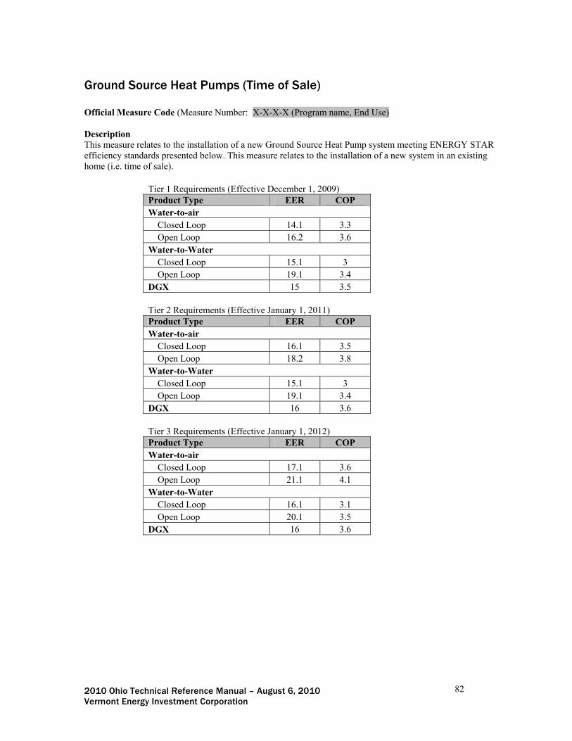
2010 Ohio Technical Reference Manual – August 6, 2010 82 Vermont Energy Investment Corporation
Ground Source Heat Pumps (Time of Sale) Official Measure Code (Measure Number: X-X-X-X (Program name, End Use) Description This measure relates to the installation of a new Ground Source Heat Pump system meeting ENERGY STAR efficiency standards presented below. This measure relates to the installation of a new system in an existing home (i.e. time of sale).
Tier 1 Requirements (Effective December 1, 2009) Product Type EER COP Water-to-air
Closed Loop 14.1 3.3 Open Loop 16.2 3.6
Water-to-Water Closed Loop 15.1 3 Open Loop 19.1 3.4
DGX 15 3.5 Tier 2 Requirements (Effective January 1, 2011) Product Type EER COP Water-to-air
Closed Loop 16.1 3.5 Open Loop 18.2 3.8
Water-to-Water Closed Loop 15.1 3 Open Loop 19.1 3.4
DGX 16 3.6 Tier 3 Requirements (Effective January 1, 2012) Product Type EER COP Water-to-air
Closed Loop 17.1 3.6 Open Loop 21.1 4.1
Water-to-Water Closed Loop 16.1 3.1 Open Loop 20.1 3.5
DGX 16 3.6

2010 Ohio Technical Reference Manual – August 6, 2010 83 Vermont Energy Investment Corporation
Definition of Efficient Equipment In order for this characterization to apply, the efficient equipment must be a Ground Source Heat Pump unit meeting the minimum ENERGY STAR efficiency level standards effective at the time of installation as detailed above. Definition of Baseline Equipment The baseline equipment is assumed to be an Air Source Heat Pump meeting the Federal Standard efficiency level; 13 SEER and 11 EER. Deemed Calculation for this Measure
Annual kWh Savings = (FLHcool * BtuH * (1/13 – (1/(EERee * 1.02))/ + (FLHheat * BtuH * (1/7.7 – (1/COPee * 3.412))/1000
Summer Coincident Peak kW Savings = BtuH * (1/11 - 1/(((EERee * 1.02) * 0.37) + 6.43))/
1000 * 0.5
Deemed Lifetime of Efficient Equipment The expected measure life is assumed to be 18 years 200. Deemed Measure Cost The actual installed cost of the Ground Source Heat Pump should be used, minus the assumed installation cost of a 3 ton standard baseline Air Source Heat Pump of $3,609201. Deemed O&M Cost Adjustments n/a Coincidence Factor The summer peak coincidence factor for this measure is assumed to be 0.5202.
REFERENCE SECTION
Calculation of Savings Energy Savings
ΔkWH = (FLHcool * BtuH * (1/SEERbase – (1/(EERee * 1.02))/1000 + (FLHheat * BtuH * (1/HSPFbase – (1/COPee * 3.412))/1000
Where:
FLHcool = Full load cooling hours Dependent on location as below:
Location Run Hours203 Akron 476
200 Measure Life Report, Residential and Commercial/Industrial Lighting and HVAC Measures, GDS Associates, June 2007. http://www.ctsavesenergy.org/files/Measure%20Life%20Report%202007.pdf 201 Based on DEER 2008 Database Technology and Measure Cost Data (www.deeresources.com). Material cost of 13 SEER AC is $796 per ton, and labor cost of $407 per ton. For a 3 ton unit this would be (796+407) *3 = $3609. 202 Based on Energy Center of Wisconsin, May 2008 metering study; “Central Air Conditioning in Wisconsin, A Compilation of Recent Field Research”, p32 203 Based on Full Load Hour assumptions taken from the ENERGY STAR calculator (http://www.energystar.gov/ia/business/bulk_purchasing/bpsavings_calc/Calc_CAC.xls) and reduced by 33% due to assumption that the average air conditioning is oversized by 50% (Neme, Proctor, Nadal, 1999; “National Energy Savings Potential From Addressing Residential HVAC Installation Problems”). Note this approach results in full load hour estimates within 10% of measured estimates from the Wisconsin study.

2010 Ohio Technical Reference Manual – August 6, 2010 84 Vermont Energy Investment Corporation
Cincinnati 664 Cleveland 426 Columbus 552
Dayton 631 Mansfield 474
Toledo 433 Youngstown 369
BtuH = Size of equipment in Btuh (note 1 ton = 12,000Btuh)
= Actual installed SEERbase = SEER Efficiency of baseline unit
= 13 204 EERee = EER Efficiency of efficient unit
= Actual installed 1.02 = Constant used to estimate the SEER based on the efficient unit’s EER205. FLHheat = Full load heating hours Dependent on location as below:
Location Run Hours206 Akron 1576
Cincinnati 1394 Cleveland 1567 Columbus 1272
Dayton 1438 Mansfield 1391
Toledo 1628 HSPFbase =Heating Season Performance Factor for baseline unit =7.7207 COPee = Coefficient of Performance of efficient unit = Actual Installed 3.413 = Constant to convert the COP of the unit to the Heating Season Performance Factor
HSPF).
For example, a 3 ton unit with EER rating of 16 and COP of 3.5 in Dayton: ΔkWH = (FLHcool * BtuH * (1/SEERbase – (1/(EERee * 1.02))/1000
+ (FLHheat * BtuH * (1/HSPFbase – (1/COPee * 3.412))/1000 ΔkWH = (631 * 36000 * (1/13 – 1/ (16*1.02))) / 1000 + (1438 * 36000 * (1/7.7 – 1/ (3.5*3.412)) /
1000 = 2744 kWh
Summer Coincident Peak Demand Savings
ΔkW = BtuH * (1/EERbase - 1/(((EERee * 1.02) * 0.37) + 6.43))/1000 * CF
204 Minimum Federal Standard; Federal Register, Vol. 66, No. 14, Monday, January 22, 2001/Rules and Regulations, p. 7170-7200. 205 Note that EERs of GSHPs are measured differently than EERs of air source heat pumps (focusing on entering water temperatures rather than ambient air temperatures). The equivalent SEER of a GSHP can be estimated by multiplying EER by 1.02, based on VEIC extrapolation of manufacturer data. 206 Heating EFLH extracted from simulations conducted for Duke Energy, OH Joint Utility TRM, October 2009; “Technical Reference Manual (TRM) for Ohio Senate Bill 221Energy Efficiency and Conservation Program and 09-512-GE-UNC” 207 Minimum Federal Standard; Federal Register, Vol. 66, No. 14, Monday, January 22, 2001/Rules and Regulations, p. 7170-7200.

2010 Ohio Technical Reference Manual – August 6, 2010 85 Vermont Energy Investment Corporation
Where: EERbase = EER Efficiency of baseline unit
= 11 208 EERee = EER Efficiency of ENERGY STAR unit
= Actual installed 1.02 = Constant used to estimate the unit’s equivalent air conditioning SEER based on the
GSHP unit’s EER209. This is then converted to the unit’s equivalent air conditioning EER to enable comparisons to the baseline unit using the following algorithm: EERac = (SEER * 0.37) + 6.43210
CF = Summer Peak Coincidence Factor for measure = 0.5211
For example, a 3 ton unit with EER rating of 16:
ΔkW = (36000 * (1/11 – 1/ (((16 * 1.02) * 0.37) + 6.43)) / 1000 * 0.5
= 0.2 kW Fossil Fuel Impact Descriptions and Calculation n/a Water Impact Descriptions and Calculation n/a Deemed O&M Cost Adjustment Calculation n/a Version Date & Revision History Draft: Portfolio # Effective date: Date TRM will become effective End date: Date TRM will cease to be effective (or TBD)
208 Minimum Federal Standard; as above. 209 Note that EERs of GSHPs are measured differently than EERs of air source heat pumps (focusing on entering water temperatures rather than ambient air temperatures). The equivalent SEER of a GSHP can be estimated by multiplying EER by 1.02, based on VEIC extrapolation of manufacturer data. 210 Roberts and Salcido, Architectural Energy Corporation, Feb 2008; “Peak Electric Demand Calculations in the REM/Rate Home Energy Rating Software and REM/Design Home Energy Analysis Software”. This formulaic relationship was derived from 1861 unique combinations of data, from nearly 200,000 ARI-rated residential central air conditioners. 211 Based on Energy Center of Wisconsin, May 2008 metering study; “Central Air Conditioning in Wisconsin, A Compilation of Recent Field Research”, p32
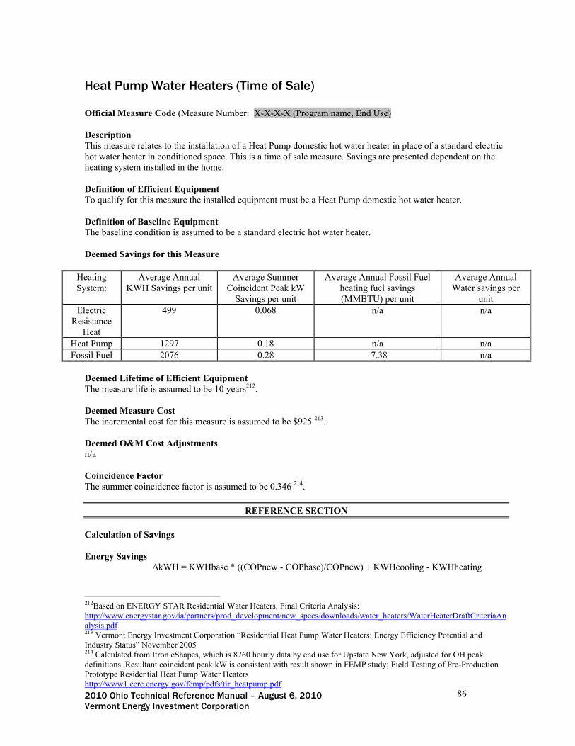
2010 Ohio Technical Reference Manual – August 6, 2010 86 Vermont Energy Investment Corporation
Heat Pump Water Heaters (Time of Sale) Official Measure Code (Measure Number: X-X-X-X (Program name, End Use) Description This measure relates to the installation of a Heat Pump domestic hot water heater in place of a standard electric hot water heater in conditioned space. This is a time of sale measure. Savings are presented dependent on the heating system installed in the home. Definition of Efficient Equipment To qualify for this measure the installed equipment must be a Heat Pump domestic hot water heater. Definition of Baseline Equipment The baseline condition is assumed to be a standard electric hot water heater. Deemed Savings for this Measure
Heating System:
Average Annual KWH Savings per unit
Average Summer Coincident Peak kW
Savings per unit
Average Annual Fossil Fuel heating fuel savings (MMBTU) per unit
Average Annual Water savings per
unit Electric
Resistance Heat
499 0.068 n/a n/a
Heat Pump 1297 0.18 n/a n/a Fossil Fuel 2076 0.28 -7.38 n/a
Deemed Lifetime of Efficient Equipment The measure life is assumed to be 10 years212. Deemed Measure Cost The incremental cost for this measure is assumed to be $925 213. Deemed O&M Cost Adjustments n/a Coincidence Factor The summer coincidence factor is assumed to be 0.346 214.
REFERENCE SECTION
Calculation of Savings Energy Savings
ΔkWH = KWHbase * ((COPnew - COPbase)/COPnew) + KWHcooling - KWHheating
212Based on ENERGY STAR Residential Water Heaters, Final Criteria Analysis: http://www.energystar.gov/ia/partners/prod_development/new_specs/downloads/water_heaters/WaterHeaterDraftCriteriaAnalysis.pdf 213 Vermont Energy Investment Corporation “Residential Heat Pump Water Heaters: Energy Efficiency Potential and Industry Status” November 2005 214 Calculated from Itron eShapes, which is 8760 hourly data by end use for Upstate New York, adjusted for OH peak definitions. Resultant coincident peak kW is consistent with result shown in FEMP study; Field Testing of Pre-Production Prototype Residential Heat Pump Water Heaters http://www1.eere.energy.gov/femp/pdfs/tir_heatpump.pdf

2010 Ohio Technical Reference Manual – August 6, 2010 87 Vermont Energy Investment Corporation
Where: KWHbase = Average electric DHW consumption
= 3460 215 COPnew = Coefficient of Performance (efficiency) of Heat Pump water heater
= 2.0 216 COPbase = Coefficient of Performance (efficiency) of standard electric water heater
= 0.904 217 KWHcooling = Cooling savings from conversion of heat in home to water heat = 180 218 KWHheating = Heating cost from conversion of heat in home to water heat.
Dependent on heating fuel as follows219: KWHheating (electric resistance) = 1,577 KWHheating (heat pump COP 2.0) = 779 KWHheating (fossil fuel) = 0
ΔkWH electric resistance heat = 3460 * ((2.0 – 0.904) / 2.0) + 180 - 1577
= 499 kWh
ΔkWH heat pump heat = 3460 * ((2.0 – 0.904) / 2.0) + 180 - 779 = 1,297 kWh
ΔkWH fossil fuel heat = 3460 * ((2.0 – 0.904) / 2.0) + 180 - 0 = 2,076 kWh
Summer Coincident Peak Demand Savings
ΔkW = ΔkWh / Hours * CF
Where: Hours = Full load hours of hot water heater
= 2533 220 CF = Summer Peak Coincidence Factor for measure
= 0.346 221
215 Assumption taken from; Residential Water Heaters Technical Support Document for the January 17, 2001, Final Rule Table 9.3.9, p9-34, http://www1.eere.energy.gov/buildings/appliance_standards/residential/pdfs/09.pdf Consistent with FEMP study; Field Testing of Pre-Production Prototype Residential Heat Pump Water Heaters http://www1.eere.energy.gov/femp/pdfs/tir_heatpump.pdf 216 Efficiency based on ENERGY STAR Residential Water Heaters, Final Criteria Analysis: http://www.energystar.gov/ia/partners/prod_development/new_specs/downloads/water_heaters/WaterHeaterDraftCriteriaAnalysis.pdf 217 As above 218 Determined by calculating the MMBtu removed from the air, applying the REMRate determined percentage (35%) of lighting savings that result in reduced cooling loads (lighting is used as a proxy for hot water heating since load shapes suggest their seasonal usage patterns are similar), assuming a SEER 11 central AC unit, multiplying by 64% to adjust for the percentage of OH homes having cooling (East North Central census division from Energy Information Administration, 2005 Residential Energy Consumption Survey; http://www.eia.doe.gov/emeu/recs/recs2005/hc2005_tables/hc6airconditioningchar/pdf/tablehc12.6.pdf), and applying the Discretionary Usage Adjustment of 0.75% (Based on Energy Center of Wisconsin, May 2008 metering study; “Central Air Conditioning in Wisconsin, A Compilation of Recent Field Research”, p31) 219 Determined by calculating the MMBtu removed from the air, as above, applying the REMRate determined percentage (45%) of lighting savings that result in increased heating loads, converting to kWh and dividing by efficiency of heating system (1.0 for electric resistance, 2.0 for heat pump). 220 Full load hours assumption based on Efficiency Vermont loadshape, calculated from Itron eShapes. 221 Calculated from Itron eShapes, which is 8760 hourly data by end use for Upstate New York, adjusted for OH peak definitions. Resultant coincident peak kW is consistent with result shown in FEMP study; Field Testing of Pre-Production Prototype Residential Heat Pump Water Heaters http://www1.eere.energy.gov/femp/pdfs/tir_heatpump.pdf

2010 Ohio Technical Reference Manual – August 6, 2010 88 Vermont Energy Investment Corporation
ΔkW electric resistance heat = 499 / 2533 * 0.346
= 0.068 kW ΔkW heat pump heat = 1297 / 2533 * 0.346
= 0.18 kW
ΔkW fossil fuel heat = 2076 / 2533 * 0.346 = 0.28 kW Fossil Fuel Impact Descriptions and Calculation (For homes with fossil fuel heating system)
ΔMMBtu = -7.38 MMBtu222
Water Impact Descriptions and Calculation n/a Deemed O&M Cost Adjustment Calculation n/a Version Date & Revision History Draft: Portfolio # Effective date: Date TRM will become effective End date: Date TRM will cease to be effective (or TBD)
222 This is the additional energy consumption (therefore a negative value) required to replace the heat removed from the home during the heating season by the heat pump water heater. Determined by calculating the MMBtu removed from the air, applying the REMRate determined percentage (45%) of lighting savings that result in increased heating loads (lighting is used as a proxy for hot water heating since load shapes suggest their seasonal usage patterns are similar), dividing by the efficiency of the heating system (estimated assuming that natural gas central furnace heating is typical for Ohio residences (65% of East North Central census division has a Natural Gas Furnace (based on Energy Information Administration, 2005 Residential Energy Consumption Survey: http://www.eia.doe.gov/emeu/recs/recs2005/hc2005_tables/hc4spaceheating/pdf/tablehc12.4.pdf)) In 2000, 40% of furnaces purchased in Ohio were condensing (based on data from GAMA, provided to Department of Energy during the federal standard setting process). Assuming typical efficiencies for condensing and non condensing furnace and duct losses, the average heating system efficiency is estimated as follows: (0.4*0.92) + (0.6*0.8) * (1-0.15) = 0.72.

2010 Ohio Technical Reference Manual – August 6, 2010 89 Vermont Energy Investment Corporation
Low Flow Faucet Aerator (Time of Sale or Early Replacement) Official Measure Code (Measure Number: X-X-X-X (Program name, End Use) Description This measure relates to the installation of a low flow (1.5 GPM) faucet aerator in a home. This could be a retrofit direct install measure or a new installation. Both electric and fossil fuel savings are provided, although only savings corresponding to the hot water heating fuel should be claimed. Definition of Efficient Equipment The efficient equipment is a low flow aerator. Definition of Baseline Equipment The baseline equipment is a standard faucet aerator using 2.2 GPM. Deemed Calculation for this Measure Annual kWh savings = ISR * ((2.2 – GPMlow) / 2.2) * 77 Summer Coincident Peak savings = ΔkWH * 0.000125 Annual MMBTU savings = ISR * ((2.2 – GPMlow) / 2.2) * 0.3435
Annual Water savings (gallons) = ISR * ((2.2 – GPMlow) / 2.2) * 1398 Deemed Lifetime of Efficient Equipment The measure life is assumed to be 5 years223. Deemed Measure Cost As a retrofit measure, the cost will be the actual cost of the aerator and its installation. As a measure distributed to, but installed by, participants, the cost will be the cost of the aerator and the distribution costs. As a time of sale measure, the cost is assumed to be $2224. Deemed O&M Cost Adjustments When a retrofit measure, there would be a very small O&M benefit associated with the deferral of the next replacement, but this has conservatively not been characterized. Coincidence Factor The coincidence factor for this measure is calculated at 0.0026225.
REFERENCE SECTION
Calculation of Savings Energy Savings If electric domestic hot water heater:
223 Conservative estimate based on review of TRM assumptions from other States. 224 Navigant Consulting, Ontario Energy Board; “Measures and Assumptions for Demand Side Management (DSM) Planning”, April 2009. 225 Calculated as follows: Assume 13% faucet use takes place during peak hours (based on: http://www.aquacraft.com/Download_Reports/DISAGGREGATED-HOT_WATER_USE.pdf) 13% * 3.6 minutes per day (10.9 * 2.56 / 3.5 / 2.2 = 3.6) = 0.47 minutes = 0.47 / 180 (minutes in peak period) = 0.00262

2010 Ohio Technical Reference Manual – August 6, 2010 90 Vermont Energy Investment Corporation
ΔkWH = ISR * ((((GPMbase - GPMlow) / GPMbase) * # people * gals/day * days/year *
DR) / F/home) * 8.3 * (Tft - Tmains) / 1,000,000) / DHW Recovery Efficiency / 0.003412
Where:
ISR = In Service Rate or fraction of units that get installed Retrofit/Direct Install = 1.0 Customer self install = 0.48226 GPMbase = Gallons Per Minute of baseline faucet
= 2.2 227 GPMlow = Gallons Per Minute of low flow faucet
= Actual # people = Average number of people per household
= 2.46 228 gals/day = Average gallons per day used by all faucets in home
= 10.9 229 days/y = Days faucet used per year
= 365 DR = Percentage of water flowing down drain (if water is collected in a sink, a faucet
aerator will not result in any saved water) = 50% 230
F/home = Average number of faucets in the home = 3.5 231
8.3 = Constant to convert gallons to lbs Tft = Assumed temperature of water used by faucet
= 80 232 Tmains = Assumed temperature of water entering house
= 57.8 233 DHW Recovery Efficiency = Recovery efficiency of electric hot water heater
= 0.98 234 0.003412 = Constant to converts MMBtu to kWh
For example, a 1.5GPM direct installation:
ΔkWH = 1.0 * ((((2.2 – 1.5) / 2.2) * 2.46 * 10.9 * 365 * 0.5)) / 3.5 * 8.3 * (80-57.8) / 1,000,000) / 0.98 / 0.003412
= 24.5 kWh
226 EGD_2009_DSM_Annual Report from table 27 survey of Install rates: Overall averages of 62% and 34% for kitchen and bath aerators respectively are averaged to get 48%. There is significant variation in rates by building type, aerator type, and distribution so surveying participants is encouraged 227 In 1998, the Department of Energy adopted a maximum flow rate standard of 2.2 gpm at 60 psi for all faucets: 63 Federal Register 13307; March 18, 1998. 228 US Energy Information Administration, Residential Energy Consumption Survey, East North Central Census Division; http://www.eia.doe.gov/emeu/recs/recs2005/hc2005_tables/hc3demographics/pdf/tablehc12.3.pdf 229 Most commonly quoted value of gallons of water used per person per day (including in U.S. Environmental Protection Agency’s “water sense” documents; http://www.epa.gov/watersense/docs/home_suppstat508.pdf) 230 Estimate consistent with Ontario Energy Board, "Measures and Assumptions for Demand Side Management Planning" 231 Estimate based on East Bay Municipal Utility District; "Water Conservation Market Penetration Study" http://www.ebmud.com/sites/default/files/pdfs/market_penetration_study_0.pdf 232 Connecticut Energy Efficiency Fund; CL&P and UI Program Savings Documentation for 2008 Program Year 233 Annual average of all cities obtained from OH Joint Utility TRM; Table 39: Monthly Mains Water Temperature for Selected Cities (°F). 234 Electric water heater have recovery efficiency of 98%: http://www.ahrinet.org/ARI/util/showdoc.aspx?doc=576

2010 Ohio Technical Reference Manual – August 6, 2010 91 Vermont Energy Investment Corporation
Summer Coincident Peak Demand Savings
ΔkW = ΔkWh/hours * CF
Where: Hours = Average number of hours per year spent using faucet
= (Gal/person * # people * 365) / F/home / GPM / 60 = (10.9 * 2.46 * 365) / 3.5 / 2.2 / 60 = 21 hours
CF = Summer Peak Coincidence Factor for measure = 0.00262
For example, a 1.5GPM direct installation:
ΔkW = 24.5 / 21 * 0.00262
= 0.0031 kW Fossil Fuel Impact Descriptions and Calculation If fossil fuel domestic hot water heater, MMBtu savings provided below:
ΔMMBtu = ISR * ((((GPMbase - GPMlow) / GPMbase) * # people * gals/day * days/year * DR) / F/home) * 8.3 * (Tft - Tmains) / 1,000,000) / Gas DHW Recovery Efficiency
Where:
Gas DHW Recovery Efficiency = Recovery efficiency of electric hot water heater = 0.75 235
For example, a 1.5GPM direct installation:
ΔMMBtu = 1.0 * ((((2.2 – 1.5) / 2.2) * 2.46 * 10.9 * 365 * 0.5)) / 3.5 * 8.3 * (80-57.8) / 1,000,000) / 0.75
= 0.109 MMBtu Water Impact Descriptions and Calculation
Water Savings = ISR * (((GPMbase - GPMlow) / GPMbase) * # people * gals/day *
days/year * DR) / F/home
For example, a 1.5GPM direct installation:
Water Savings = 1.0 * ((((2.2 – 1.5) / 2.2) * 2.46 * 10.9 * 365 * 0.5)) / 3.5 = 445 gallons Deemed O&M Cost Adjustment Calculation When a retrofit measure, there would be a very small O&M benefit associated with the deferral of the next replacement, but this has conservatively not been characterized.
235 Review of AHRI Directory suggests range of recovery efficiency ratings for new Gas DHW units of 70-87%. Average of existing units is estimated at 75%

2010 Ohio Technical Reference Manual – August 6, 2010 92 Vermont Energy Investment Corporation
Version Date & Revision History Draft: Portfolio # Effective date: Date TRM will become effective End date: Date TRM will cease to be effective (or TBD)

2010 Ohio Technical Reference Manual – August 6, 2010 93 Vermont Energy Investment Corporation
Low Flow Showerhead (Time of Sale or Early Replacement) Official Measure Code (Measure Number: X-X-X-X (Program name, End Use) Description This measure relates to the installation of a low flow showerhead in a home. This is a retrofit direct install measure or a new installation. Both electric and fossil fuel savings are provided, although only savings corresponding to the hot water heating fuel should be claimed. Definition of Efficient Equipment The efficient condition is a low flow showerhead. Definition of Baseline Equipment The baseline is a standard showerhead using 2.87 GPM236. Deemed Calculation for this Measure Annual kWh savings = ISR * (2.87 – GPMlow) * 179 Summer Coincident Peak savings = ΔkWH * 0.000112 Annual MMBTU savings = ISR * (2.87 – GPMlow) * 0.8
Annual Water savings (gal) = ISR * ((2.87 – GPMlow) / 2.87) * 4960
Deemed Lifetime of Efficient Equipment The measure life is assumed to be 5 years 237. Deemed Measure Cost As a retrofit measure, the incremental cost will be the cost of the showerhead including its installation. As a measure distributed to, but installed by, participants, the cost will be the cost of the showerhead and the distribution costs. As a time of sale measure, the incremental cost is assumed to be $6238. Deemed O&M Cost Adjustments When a retrofit measure, there would be a very small O&M benefit associated with the deferral of the next replacement, but this has conservatively not been characterized. Coincidence Factor The coincidence factor for this measure is calculated at 0.00371 239.
236 Average flow rate of replaced showerhead from Enbridge Gas Distribution Inc., April 2010; “Demand Side Management 2009 DSM Draft Annual Report”, p77-78. Calculated with the average flow rate of units between 2 and 2.5GPM of 2.45GPM, average flow rate of units greater than 2.5GPM of 3.07, and 33% of all units between 2 and 2.5%, 67% of units over 2.5GPM; (2.45*0.33)+(3.07*0.67) = 2.87GPM 237 Conservative estimate based on review of TRM assumptions from other States. 238 Navigant Consulting, Ontario Energy Board, “Measures and Assumptions for Demand Side Management (DSM) Planning”, April 2009. 239 Calculated as follows: Assume 9% showers take place during peak hours (based on: http://www.aquacraft.com/Download_Reports/DISAGGREGATED-HOT_WATER_USE.pdf) 9% * 7.42 minutes per day (11.6 * 2.56 / 1.6 / 2.5 = 7.42) = 0.668 minutes = 0.668 / 180 (minutes in peak period) = 0.00371

2010 Ohio Technical Reference Manual – August 6, 2010 94 Vermont Energy Investment Corporation
REFERENCE SECTION
Calculation of Savings Energy Savings If electric domestic hot water heater:
ΔkWH = ISR * (GPMbase – GPMlow) * kWh/GPMreduced
Where: ISR = In Service Rate or fraction of units that get installed Retrofit/Direct Install = 1.0 Customer self install = 0.81240 GPMbase = Gallons Per Minute of baseline showerhead
= 2.87 241 GPMlow = Gallons Per Minute of low flow showerhead
= Actual kWh/GPMreduced = Assumed kWh savings per GPM reduction = 149kWh per gallon reduced242
For example, a 2.0 GPM direct installation:
ΔkWH = 1.0 * (2.87 – 2.0) * 149
= 130 kWh
Summer Coincident Peak Demand Savings If electric domestic hot water heater:
ΔkW = ΔkWh/Hours * CF
Where:
Hours = Average number of hours per year spent using shower head = (Gal/person * # people * days/y) / SH/home / GPM / 60
gals/day = Average gallons per day used for showering = 11.6 243
# people = Average number of people per household = 2.46 244
days/y = Days shower used per year = 365
240 EGD_2009_DSM_Annual Report from table 27 survey of Install rates: Overall averages 81%. There may be significant variations due to specifics of the program distribution, so surveying participants is encouraged. 241 The Energy Policy Act of 1992 (EPAct) established the maximum flow rate for showerheads at 2.5 gallons per minute (gpm). 242 This is based on an Enbridge metering study (Enbridge Gas Distribution Inc., April 2010; “Demand Side Management 2009 DSM Draft Annual Report”, p75) that found 46m3 of natural gas savings when replacing all existing showerheads (with average flow rate of 2.45 GPM) with 1.25GPM showerheads (the replacement GPM and the number of showers per home (2.1) were determined during personal conversations with study authors). This equates to 0.66MMBtu of savings per showerhead per 1GPM reduction. This is converted to kWh by multiplying by the recovery efficiency of a gas heater (0.75 based on review of AHRI Directory) over the recovery efficiency of an electric heater (0.98 from: http://www.ahrinet.org/ARI/util/showdoc.aspx?doc=576) and multiplying by 293 (kWh/MMBtu). 243 Most commonly quoted value of gallons of water used per person per day (including in U.S. Environmental Protection Agency’s “water sense” documents; http://www.epa.gov/watersense/docs/home_suppstat508.pdf) 244 US Energy Information Administration, Residential Energy Consumption Survey, East North Central Census Division; http://www.eia.doe.gov/emeu/recs/recs2005/hc2005_tables/hc3demographics/pdf/tablehc12.3.pdf

2010 Ohio Technical Reference Manual – August 6, 2010 95 Vermont Energy Investment Corporation
Showers/home = Average number of showers in the home = 2.1 245
= (11.6 * 2.46 * 365) / 2.1 / 2.87 / 60 = 29 hours
CF = Summer Peak Coincidence Factor for measure = 0.00371 246
For example, a 2.0 GPM direct installation:
ΔkW = 130 / 29 * 0.00371
= 0.017 kW Fossil Fuel Impact Descriptions and Calculation If fossil fuel domestic hot water heater:
ΔMMBtu = ISR * (GPMbase – GPMlow) * MMBtu/GPMreduced Where:
MMBtu/GPMreduced = Assumed MMBtu savings per GPM reduction = 0.66 MMBtu per gallon reduced 247
For example, a 2.0 GPM direct installation:
ΔMMBtu = 1.0 * (2.87 – 2.0) * 0.66 = 0.6 MMBtu Water Impact Descriptions and Calculation
Water Savings = ISR * (((GPMbase - GPMlow) / GPMbase) * # people * gals/day * days/year)) / SH/home
For example, a 2.0 GPM direct installation:
Water Savings = 1.0* ((((2.87 – 2.0) / 2.87) * 2.46 * 11.6 * 365)) / 2.1 = 1,504 gallons Deemed O&M Cost Adjustment Calculation When a retrofit measure, there would be a very small O&M benefit associated with the deferral of the next replacement, but this has conservatively not been characterized.
245 Personal communication with authors of Enbridge Gas Distribution Inc., April 2010; “Demand Side Management 2009 DSM Draft Annual Report” 246 Calculated as follows: Assume 9% showers take place during peak hours (based on: http://www.aquacraft.com/Download_Reports/DISAGGREGATED-HOT_WATER_USE.pdf) 9% * 7.42 minutes per day (11.6 * 2.56 / 1.6 / 2.5 = 7.42) = 0.668 minutes = 0.668 / 180 (minutes in peak period) = 0.00371 247 This is based on an Enbridge metering study (Enbridge Gas Distribution Inc., April 2010; “Demand Side Management 2009 DSM Draft Annual Report”, p75) that found 46m3 of natural gas savings when replacing all existing showerheads (with average flow rate of 2.45 GPM) with 1.25GPM showerheads (the replacement GPM and the number of showers per home (2.1) were determined during personal conversations with study authors). This equates to 0.66MMBtu of savings per showerhead per 1GPM reduction.

2010 Ohio Technical Reference Manual – August 6, 2010 96 Vermont Energy Investment Corporation
Version Date & Revision History Draft: Portfolio # Effective date: Date TRM will become effective End date: Date TRM will cease to be effective (or TBD)

2010 Ohio Technical Reference Manual – August 6, 2010 97 Vermont Energy Investment Corporation
Domestic Hot Water Pipe Insulation (Retrofit) Official Measure Code (Measure Number: X-X-X-X (Program name, End Use) Description This measure describes adding insulation to un-insulated domestic hot water pipes. The measure assumes the pipe wrap is installed to the first length of both the hot and cold pipe up to the first elbow. Definition of Efficient Equipment To efficiency case is installing pipe wrap insulation to a length of hot water carrying copper pipe. Definition of Baseline Equipment The baseline is an un-insulated hot water carrying copper pipe. Deemed Calculation for this Measure
Annual kWh savings (electric DHW systems) = ((1 – 1/Rnew) * (L * C) * 170.2
Summer Coincident Peak Savings (electric DHW systems) = ΔkWh/8760
Annual MMBtu savings (fossil fuel DHW systems) = ((1 – 1/Rnew) * (L * C) * 0.569
Deemed Lifetime of Efficient Equipment The measure life is assumed to be 15 years 248. Deemed Measure Cost The measure cost including material and installation is assumed to be $3 per linear foot249. Deemed O&M Cost Adjustments n/a Coincidence Factor This measure assumes a flat loadshape and as such the coincidence factor is 1.
REFERENCE SECTION
Calculation of Savings Energy Savings For electric DHW systems:
ΔkWh = ((1/Rexist – 1/Rnew) * (L * C) * ΔT * 8,760)/ ηDHW / 3413
Where:
Rexist = Pipe heat loss coefficient of uninsulated pipe (existing) (Btu/hr-°F-ft) = 1.0250
Rnew = Pipe heat loss coefficient of insulated pipe (new) (Btu/hr-°F-ft)
248 Measure Life Report, Residential and Commercial/Industrial Lighting and HVAC Measures, GDS Associates, June 2007. http://www.ctsavesenergy.org/files/Measure%20Life%20Report%202007.pdf 249 Consistent with DEER 2008 Database Technology and Measure Cost Data (www.deeresources.com). 250 Navigant Consulting Inc., April 2009; “Measures and Assumptions for Demand Side Management (DSM) Planning; Appendix C Substantiation Sheets”, p77.

2010 Ohio Technical Reference Manual – August 6, 2010 98 Vermont Energy Investment Corporation
= Actual L = Length of pipe from water heating source covered by pipe wrap (ft) = actual C = Circumference of pipe (ft) (Diameter (in) * π * 0.083) = actual (0.5” pipe = 0.13ft, 0.75” pipe = 0.196ft) ΔT = Average temperature difference between supplied water and outside air
temperature (°F) = 65°F 251 8,760 = Hours per year ηDHW = Recovery efficiency of electric hot water heater
= 0.98 252 3413 = Conversion from Btu to kWh
For example, insulating 5 feet of 0.75” pipe with R-4 wrap:
ΔkWh = ((1/Rexist – 1/Rnew) * (L * C) * ΔT * 8,760) / ηDHW / 3413 = ((1/1– 1/5) * (5 * 0.196) * 65 * 8760) / 0.98 /3413 = 133 kWh Summer Coincident Peak Demand Savings
ΔkW = ΔkWh/8760
Where: ΔkWh = kWh savings from pipe wrap installation 8760 = Number of hours in a year (since savings are assumed to be constant over year).
For example, insulating 5 feet of 0.75” pipe with R-4 wrap:
ΔkW = 133/8760 = 0.015kW Fossil Fuel Impact Descriptions and Calculation For fossil fuel DHW systems:
ΔMMBtu = ((1/Rexist – 1/Rnew) * (L * C) * ΔT * 8,760) / ηDHW /1,000,000
Where: ηDHW = Recovery efficiency of gas hot water heater
= 0.75 253 For example, insulating 5 feet of 0.75” pipe with R-4 wrap: ΔMMBtu = ((1/1– 1/5) * (5 * 0.196) * 65 * 8760) / 0.75 / 1,000,000 = 0.60 MMBtu
251 Assumes 130°F water leaving the hot water tank and average temperature of basement of 65°F. 252 Electric water heater have recovery efficiency of 98%: http://www.ahrinet.org/ARI/util/showdoc.aspx?doc=576 253 Review of AHRI Directory suggests range of recovery efficiency ratings for new Gas DHW units of 70-87%. Average of existing units is estimated at 75%
2010 Ohio Technical Reference Manual – August 6, 2010 99 Vermont Energy Investment Corporation
Water Impact Descriptions and Calculation n/a Deemed O&M Cost Adjustment Calculation n/a Version Date & Revision History Draft: Portfolio # Effective date: Date TRM will become effective End date: Date TRM will cease to be effective (or TBD)
2010 Ohio Technical Reference Manual – August 6, 2010 100 Vermont Energy Investment Corporation
Wall Insulation (Retrofit) Official Measure Code (Measure Number: X-X-X-X (Program name, End Use) Description This measure characterization is for the installation of new additional insulation in the walls of a residential building. The measure assumes that an auditor, contractor or utility staff member is on location, and will measure and record the existing and new insulation depth and type (to calculate R-values), the surface area of insulation added, and the efficiency of the heating system used in the home. Definition of Efficient Equipment The new insulation should meet any qualification criteria required for participation in the program. The new insulation R-value should include the total wall assembly and include any existing insulation that is left in situ. Definition of Baseline Equipment The existing insulation R-value should include the total wall assembly. An R-value of 5 should be assumed for the wall assembly plus the R-value of any existing insulation254. Deemed Calculation for this Measure Air conditioning Savings
Annual kWh Savings = ((1/Rexist – 1/Rnew) * CDH * 0.75 * Area) / 1000 / ηCool Summer Coincident Peak kW Savings = ΔkWh / FLHcool * 0.5 Space Heating Savings:
Annual MMBTU Savings (fossil fuel heating) = ((1/Rexist – 1/Rnew) * HDD * 24 * Area) / 1,000,000 / ηHeat
Annual kWh Savings (electric heating)
= (((1/Rexist – 1/Rnew) * HDD * 24 * Area) / 1,000,000 / ηHeat) * 293.1 Deemed Lifetime of Efficient Equipment The measure life is assumed to be 25 years 255. Deemed Measure Cost The actual insulation installation measure cost should be used. Deemed O&M Cost Adjustments n/a Coincidence Factor The summer peak coincidence factor for this measure is assumed to be 0.5256.
254 The R-5 assumption for wall assembly is based on J.Neymark & Associates and National Renewable Energy Laboratory, June 2009; “BESTEST-EX Interim Test Procedure” p25. 255 Measure Life Report, Residential and Commercial/Industrial Lighting and HVAC Measures, GDS Associates, June 2007. http://www.ctsavesenergy.org/files/Measure%20Life%20Report%202007.pdf 256 Based on Energy Center of Wisconsin, May 2008 metering study; “Central Air Conditioning in Wisconsin, A Compilation of Recent Field Research”, p32

2010 Ohio Technical Reference Manual – August 6, 2010 101 Vermont Energy Investment Corporation
REFERENCE SECTION
Calculation of Savings Energy Savings
ΔkWh = ((1/Rexist – 1/Rnew) * CDH * DUA * Area) / 1000 / ηCool
Where: Rexist = existing effective whole-assembly thermal resistance value or R-value257 = actual recorded Rnew = new total effective whole-assembly thermal resistance value or R-value258 = actual recorded
CDH = Cooling Degree Hours259. Dependent on location:
Location Cooling Degree Hours (75°F set point)
Akron 3,986 Cincinnati 7,711 Cleveland 5,817 Columbus 4,367
Dayton 5,934 Toledo 4,401
Youngtown 3,689 DUA = Discretionary Use Adjustment to account for the fact that people do not always
operate their air conditioning system when the outside temperature is greater than 75°F
= 0.75 260 Area = Square footage of insulated area = actual recorded ηCool = Efficiency of Air Conditioning equipment = actual recorded
For example, insulating 300 square feet of wall area from R-5 to R-20, in a Cincinnati home with AC SEER 10:
ΔkWh = ((1/Rexist – 1/Rnew) * CDH * DUA * Area) / 1000 / ηCool
= ((1/5 – 1/20) * 7711 * 0.75 * 300) / 1000 / 10
= 26 kWh
Summer Coincident Peak Demand Savings ΔkW = ΔkWh / FLHcool *CF Where:
FLHcool = Full load cooling hours
Dependent on location as below:
257 If uninsulated assembly assume R-5. 258 Include the R-value for any existing insulation remaining. 259 Derived by summing the delta between the average outdoor temperature and the base set point of 75 degrees (above which cooling is assumed to be used) each hour of the year. Hourly temperature data obtained from TMY3 data (http://rredc.nrel.gov/solar/) 260 Based on Energy Center of Wisconsin, May 2008 metering study; “Central Air Conditioning in Wisconsin, A Compilation of Recent Field Research”, p31

2010 Ohio Technical Reference Manual – August 6, 2010 102 Vermont Energy Investment Corporation
Location Run Hours261 Akron 476
Cincinnati 664 Cleveland 426 Columbus 552
Dayton 631 Mansfield 474
Toledo 433 Youngstown 369
CF = Summer Peak Coincidence Factor for measure
= 0.5262 For example, insulating 300 square feet of an attic floor from R-5 to R-20, in a Cincinnati home with AC SEER 10: ΔkW = ΔkWh / FLHcool *CF = 26 / 747 * 0.5 = 0.017 kW Space Heating Savings Calculation
ΔMMBTU = ((1/Rexist – 1/Rnew) * HDD * 24 * Area) / 1,000,000 / ηHeat
Where: HDD = Heating Degree Days (60° base temperature) for location263
Location Heating Degree Days (60°F base temperature)
Akron 4,848 Cincinnati 3,853 Cleveland 4,626 Columbus 4,100
Dayton 4,430 Toledo 4,482
Youngtown 4,887
ηHeat = Average Net Heating System Efficiency (Equipment Efficiency * Distribution Efficiency) 264
261 Based on Full Load Hour assumptions taken from the ENERGY STAR calculator (http://www.energystar.gov/ia/business/bulk_purchasing/bpsavings_calc/Calc_CAC.xls) and reduced by 33% due to assumption that the average air conditioning is oversized by 50% (Neme, Proctor, Nadal, 1999; “National Energy Savings Potential From Addressing Residential HVAC Installation Problems”). Note this approach results in full load hour estimates within 10% of measured estimates from the Energy Center of Wisconsin, May 2008 study; “Central Air Conditioning in Wisconsin, A Compilation of Recent Field Research.” 262 Based on Energy Center of Wisconsin, May 2008 metering study; “Central Air Conditioning in Wisconsin, A Compilation of Recent Field Research”, p32 263 The 10 year average annual heating degree day value, using a balance point for heating equipment use of 60 degrees was calculated for each location based on data obtained from http://www.engr.udayton.edu/weather/. The 60 degree balance point is used based on a PRISM evaluation of approximately 600,000 Ohio residential single family customers. 264 The System Efficiency can be obtained either by recording the AFUE of the unit, or performing a steady state efficiency test. The Distribution Efficiency can be estimated via a visual inspection and by referring to a look up table such as that provided by the Building Performance Institute: (http://www.bpi.org/files/pdf/DistributionEfficiencyTable-BlueSheet.pdf) or by performing duct blaster testing. If there are more than one heating systems, the weighted (by consumption) average efficiency should be used. If the heating system or distribution is being upgraded within a package of measures together with the insulation upgrade, the new average heating system efficiency should be used.

2010 Ohio Technical Reference Manual – August 6, 2010 103 Vermont Energy Investment Corporation
= actual recorded Note for homes with electric heat (resistance or heat pump), follow the MMBTU formula above and convert to kWh by multiplying by 293.1. For heat pumps the equipment efficiency used in the above algorithm should be the Coefficient Of Performance or COP (i.e., divide HSPF by 3.412; e.g., HSPF 7.7 is COP of 2.26). For example, insulating 300 square feet of an attic floor from R-5 to R-20, in a Cincinnati home with heating system efficiency of 70%:
ΔMMBTU = ((1/Rexist – 1/Rnew) * HDD * 24 * Area) / 1,000,000 / ηHeat
= ((1/5 – 1/20) * 3,992 * 24 * 300) / 1,000,000 / 0.7 = 6.2 MMBtu
Water Impact Descriptions and Calculation n/a Deemed O&M Cost Adjustment Calculation n/a Version Date & Revision History Draft: Portfolio # Effective date: Date TRM will become effective End date: Date TRM will cease to be effective (or TBD)
2010 Ohio Technical Reference Manual – August 6, 2010 104 Vermont Energy Investment Corporation
Air Sealing - Reduce Infiltration (Retrofit) Official Measure Code (Measure Number: X-X-X-X (Program name, End Use) Description This measure characterization is for the improvement of a building’s air-barrier, which together with its insulation defines the thermal boundary of the conditioned space. Air-leakage in buildings represents from 5% to 40% of the space conditioning costs265 but is also very difficult to control. The measure assumes that a trained auditor, contractor or utility staff member is on location, and will measure and record the existing air-leakage rate266 and post air-sealing leakage using a blower door, and the efficiency of the heating and cooling system used in the home. Definition of Efficient Equipment Air sealing materials and diagnostic testing should meet all eligibility program qualification criteria. The initial and final tested leakage rates should be performed in such a manner that the identified reductions can be properly discerned, particularly in situations wherein multiple building envelope measures may be implemented simultaneously. Definition of Baseline Equipment The existing air leakage should be determined through approved and appropriate test methods. The baseline condition of a building upon first inspection significantly impacts the opportunity for cost-effective energy savings through air-sealing. Deemed Calculation for this Measure
Annual Cooling kWh Savings = (((CFM50Exist – CFM50New) / 29.4) *60 * CDH * 0.0135) / 1000 / ηCool
Summer Coincident Peak kW Savings = ΔkWh / FLHcool * 0.5 Space Heating Savings:
MMBTU Savings (fossil fuel heating) = (((CFM50Exist – CFM50New) / N-factor) *60 * 24 * HDD * 0.018) / 1,000,000 / ηHeat
kWh Savings (electric heating) = ((((CFM50Exist – CFM50New) / N-factor) *60 * 24 * HDD *
0.018) / 1,000,000 / ηHeat) * 293.1
Deemed Lifetime of Efficient Equipment The measure life is assumed to be 15 years267. Deemed Measure Cost The actual air sealing measure cost should be used. Deemed O&M Cost Adjustments n/a
265 Krigger, J. Dorsi, C. “Residential Energy” 2004, p.73 266 In accordance with industry best practices see: BPI Building Analyst and Envelope Professional standards, http://www.bpi.org/standards_approved.aspx 267 Measure Life Report, Residential and Commercial/Industrial Lighting and HVAC Measures, GDS Associates, June 2007. http://www.ctsavesenergy.org/files/Measure%20Life%20Report%202007.pdf

2010 Ohio Technical Reference Manual – August 6, 2010 105 Vermont Energy Investment Corporation
Coincidence Factor The summer peak coincidence factor for this measure is assumed to be 0.5268.
REFERENCE SECTION
Calculation of Savings Energy Savings (Space Cooling – if home has Central AC)
ΔkWh = (((CFM50Exist – CFM50New) / N-factor) *60 * CDH * DUA * 0.018) / 1000 / ηCool
Where:
CFM50Exist = Existing Cubic Feet per Minute at 50 Pascal pressure differential as measured by the blower door before airsealing.
= actual recorded CFM50New = New Cubic Feet per Minute at 50 Pascal pressure differential as measured
by the blower door after airsealing. = actual recorded
N-Factor = Conversion factor to convert 50-pascal air flows to natural airflow. = 29.4269
60 = Constant to convert cubic feet per minute to cubic feet per hour CDH = Cooling Degree Hours270.
Dependent on location: Location Cooling Degree Hours
(75°F set point) Akron 3,986
Cincinnati 7,711 Cleveland 5,817 Columbus 4,367
Dayton 5,934 Toledo 4,401
Youngtown 3,689 DUA = Discretionary Use Adjustment to account for the fact that people do not
always operate their air conditioning system when the outside temperature is greater than 75°F
= 0.75 271 0.018 = The volumetric heat capacity of air (Btu/ft3°F) ηCool = Efficiency of Air Conditioning equipment = actual recorded
For example, reducing air leakage in a Toledo home from 5000CFM50 to 3500CFM50, with SEER 10 AC:
ΔkWh = (((5000 – 3500) / 29.4) * 60 * 4401 * 0.75 * 0.018) / 1,000 / 10
268 Based on Energy Center of Wisconsin, May 2008 metering study; “Central Air Conditioning in Wisconsin, A Compilation of Recent Field Research”, p32 269 Maximum n-factor from methodology developed by the Lawrence Berkeley Laboratory (LBL), since minimal stack effect for cooling savings. 270 Derived by summing the delta between the average outdoor temperature and the base set point of 75 degrees (above which cooling is assumed to be used) each hour of the year. Hourly temperature data obtained from TMY3 data (http://rredc.nrel.gov/solar/) 271 Based on Energy Center of Wisconsin, May 2008 metering study; “Central Air Conditioning in Wisconsin, A Compilation of Recent Field Research”, p31

2010 Ohio Technical Reference Manual – August 6, 2010 106 Vermont Energy Investment Corporation
= 18 kWh Summer Coincident Peak Demand Savings ΔkW = ΔkWh / FLHcool * CF Where:
FLHcool = Full load cooling hours Dependent on location as below:
Location Run Hours272 Akron 476
Cincinnati 664 Cleveland 426 Columbus 552
Dayton 631 Mansfield 474
Toledo 433 Youngstown 369
CF = Summer Peak Coincidence Factor for measure = 0.5273
For example, reducing air leakage in a Toledo home from 5000CFM50 to 3500CFM50, with SEER 10 AC: ΔkW = 18 / 428 * 0.5 = 0.021 kW Space Heating Savings Calculation
ΔMMBTU = (((CFM50Exist – CFM50New) / N-factor) *60 * 24 * HDD * 0.018) / 1,000,000 / ηHeat
Where:
HDD = Heating Degree Days (60° base temperature) for location274 Location Heating Degree Days
(60°F base temperature) Akron 4,848
Cincinnati 3,853 Cleveland 4,626 Columbus 4,100
Dayton 4,430 Toledo 4,482
Youngtown 4,887
272 Based on Full Load Hour assumptions taken from the ENERGY STAR calculator (http://www.energystar.gov/ia/business/bulk_purchasing/bpsavings_calc/Calc_CAC.xls) and reduced by 33% due to assumption that the average air conditioning is oversized by 50% (Neme, Proctor, Nadal, 1999; “National Energy Savings Potential From Addressing Residential HVAC Installation Problems”). Note this approach results in full load hour estimates within 10% of measured estimates from the Energy Center of Wisconsin, May 2008 study; “Central Air Conditioning in Wisconsin, A Compilation of Recent Field Research.” 273 Based on Energy Center of Wisconsin, May 2008 metering study; “Central Air Conditioning in Wisconsin, A Compilation of Recent Field Research”, p32 274 The 10 year average annual heating degree day value, using a balance point for heating equipment use of 60 degrees was calculated for each location based on data obtained from http://www.engr.udayton.edu/weather/. The 60 degree balance point is used based on a PRISM evaluation of approximately 600,000 Ohio residential single family customers.

2010 Ohio Technical Reference Manual – August 6, 2010 107 Vermont Energy Investment Corporation
ηHeat = Average Net Heating System Efficiency (Equipment Efficiency * Distribution Efficiency) 275 = actual recorded
For example, reducing air leakage in a 2 story, well-shielded Toledo home from 5000CFM50 to 3500CFM50, with a gas heating system with efficiency of 70%: ΔMMBTU = (((5000 – 3500) / 17.8) * 60 * 24 * 4569 * 0.018) / 1,000,000 / 0.7
= 14.3 MMBtu
Note for homes with electric heat (resistance or heat pump), follow the MMBTU formula above and convert to kWh by multiplying by 293.1. For heat pumps the equipment efficiency used in the above algorithm should be the Coefficient Of Performance or COP (i.e., divide HSPF by 3.412; e.g., HSPF 7.7 is COP of 2.26). For example, reducing air leakage in a 2-story, well-shielded Toledo home from 5000CFM50 to 3500CFM50, with electric resistance heating:
ΔMMBTU = ((((5000 – 3500) / 17.8) * 60 * 24 * 4569 * 0.018) / 1,000,000 / 1.0) * 293.1 = 2925kWh
Water Impact Descriptions and Calculation n/a Deemed O&M Cost Adjustment Calculation n/a Version Date & Revision History Draft: Portfolio # Effective date: Date TRM will become effective End date: Date TRM will cease to be effective (or TBD)
275 The System Efficiency can be obtained either by recording the AFUE of the unit, or performing a steady state efficiency test. The Distribution Efficiency can be estimated via a visual inspection and by referring to a look up table such as that provided by the Building Performance Institute: (http://www.bpi.org/files/pdf/DistributionEfficiencyTable-BlueSheet.pdf) or by performing duct blaster testing. If there is more than one heating system, the weighted (by consumption) average efficiency should be used. If the heating system or distribution is being upgraded within a package of measures together with the insulation upgrade, the new average heating system efficiency should be used. In the case of electric heat use 1.0 as the heating system efficiency, and for heat pumps use COP (HSPF/3.412).

2010 Ohio Technical Reference Manual – August 6, 2010 108 Vermont Energy Investment Corporation
Duct Sealing (Retrofit) Official Measure Code (Measure Number: X-X-X-X (Program name, End Use) Description This measure describes evaluating the savings associated with performing duct sealing using mastic sealant or metal tape (meeting U.L. 181 requirements) to the distribution system of homes with either central air conditioning or a ducted heating system. Two methodologies for estimating the savings associate from sealing the ducts are provided. The first preferred method requires the use of a blower door and the second requires careful inspection of the duct work.
1. Modified Blower Door Subtraction – this technique is described in detail on p44 of the Energy Conservatory Blower Door Manual; http://www.energyconservatory.com/download/bdmanual.pdf
2. Evaluation of Distribution Efficiency – this methodology requires the evaluation of three duct
characteristics below, and use of the Building Performance Institutes ‘Distribution Efficiency Look-Up Table’; http://www.bpi.org/files/pdf/DistributionEfficiencyTable-BlueSheet.pdf
a. Percentage of duct work found within the conditioned space b. Duct leakage evaluation c. Duct insulation evaluation
Definition of Efficient Equipment The efficient condition is sealed duct work throughout the unconditioned space in the home. Definition of Baseline Equipment The existing baseline condition is leaky duct work within the unconditioned space in the home. Deemed Calculation for this Measure
Annual kWh savings = (((CFM50Whole House – CFM50Envelope Only) * SCF)before – (CFM50Whole House – CFM50Envelope Only) * SCF)after) * 60 * CDH * 0.0135) / 1000 / ηCool
Or = ((DEafter – DEbefore)/ DEafter)) * FLHcool * BtuH * (1/SEER)/1000
Summer Coincident Peak kW savings = ΔkWh / FLHcool * 0.5
Annual MMBtu savings (fossil fuel) = (((CFM50Whole House – CFM50Envelope Only) * SCF)before – (CFM50Whole House – CFM50Envelope Only) * SCF)after) * 60 * 24 * HDD * 0.018) / 1,000,000 / ηHeat
Annual MMBtu savings (electric) = ((((CFM50Whole House – CFM50Envelope Only) * SCF)before –

2010 Ohio Technical Reference Manual – August 6, 2010 109 Vermont Energy Investment Corporation
(CFM50Whole House – CFM50Envelope Only) * SCF)after) * 60 * 24 * HDD * 0.018) / 1,000,000 / ηHeat) * 293.1
Or Annual MMBtu savings (fossil fuel) = ((DEafter – DEbefore)/ DEafter)) * 71.2 Annual MMBtu savings (electric) = ((DEafter – DEbefore)/ DEafter)) * FLHheat * BtuH *
(1/COP * 3.413)/1000
Deemed Lifetime of Efficient Equipment The assumed lifetime of this measure is 20 years276. Deemed Measure Cost The actual duct sealing measure cost should be used. Deemed O&M Cost Adjustments n/a Coincidence Factor The summer peak coincidence factor for this measure is assumed to be 0.5277.
REFERENCE SECTION
Calculation of Savings Energy Savings Methodology 1: Modified Blower Door Subtraction Determine Duct Leakage rate before and after performing duct sealing: Duct Leakage (CFM50DL) = (CFM50Whole House – CFM50Envelope Only) * SCF Where:
CFM50Whole House = Standard Blower Door test result finding Cubic Feet per Minute at 50 Pascal pressure differential
CFM50Envelope Only = Blower Door test result finding Cubic Feet per Minute at 50 Pascal
pressure differential with all supply and return registers sealed.
SCF = Subtraction Correction Factor to account for underestimation of duct leakage due to connections between the duct system and the home. Determined by measuring pressure in duct system with registers sealed and using look up table provided by Energy Conservatory.
Calculate Energy Savings:
ΔkWhcooling = ((CFM50DL before - CFM50DL after) * 60 * CDH * DUA * 0.018) / 1000 / ηCool
276 Measure Life Report, Residential and Commercial/Industrial Lighting and HVAC Measures, GDS Associates, June 2007. http://www.ctsavesenergy.org/files/Measure%20Life%20Report%202007.pdf 277 Based on Energy Center of Wisconsin, May 2008 metering study; “Central Air Conditioning in Wisconsin, A Compilation of Recent Field Research”, p32

2010 Ohio Technical Reference Manual – August 6, 2010 110 Vermont Energy Investment Corporation
Where: CFM50DL before = Duct Leakage rate before duct sealing = calculated as above
CFM50DL after = Duct Leakage rate after duct sealing = calculated as above
60 = Constant to convert cubic feet per minute to cubic feet per hour CDH = Cooling Degree Hours278.
Dependent on location:
Location Cooling Degree Hours (75°F set point)
Akron 3,986 Cincinnati 7,711 Cleveland 5,817 Columbus 4,367
Dayton 5,934 Toledo 4,401
Youngtown 3,689 DUA = Discretionary Use Adjustment to account for the fact that people do not
always operate their air conditioning system when the outside temperature is greater than 75°F
= 0.75 279 0.018 = The volumetric heat capacity of air (Btu/ft3°F) ηCool = Efficiency of Air Conditioning equipment
= Actual For example, duct sealing in a house in Akron with SEER 11 central air conditioning and the following blower door test results:
Before: CFM50Whole House = 4800 CFM50 CFM50Envelope Only = 4500CFM50 House to duct pressure of 45 Pascals. = 1.29 SCF (Energy Conservatory look up table)
After: CFM50Whole House = 4700 CFM50
CFM50Envelope Only = 4500CFM50 House to duct pressure of 43 Pascals = 1.39 SCF (Energy Conservatory look up table)
Duct Leakage:
CFM50DL before = (4800 – 4500) * 1.29 = 387 CFM
CFM50DL after = (4700 – 4500) * 1.39
= 278 CFM Energy Savings:
ΔkWh = ((387 – 278) * 60 * 3986 * 0.75* 0.018) / 1000 / 11 = 32 kWh
278 Derived by summing the delta between the average outdoor temperature and the base set point of 75 degrees (above which cooling is assumed to be used) each hour of the year. Hourly temperature data obtained from TMY3 data (http://rredc.nrel.gov/solar/) 279 Based on Energy Center of Wisconsin, May 2008 metering study; “Central Air Conditioning in Wisconsin, A Compilation of Recent Field Research”, p31

2010 Ohio Technical Reference Manual – August 6, 2010 111 Vermont Energy Investment Corporation
Methodology 2: Evaluation of Distribution Efficiency Determine Distribution Efficiency by evaluating duct system before and after duct sealing using Building Performance Institute “Distribution Efficiency Look-Up Table”
ΔkWh cooling = ((DEafter – DEbefore)/ DEafter)) * FLHcool * BtuH * (1/SEER)/1000 Where:
DEafter = Distribution Efficiency after duct sealing DEbefore = Distribution Efficiency before duct sealing FLHcool = Full load cooling hours Dependent on location as below:
Location Run Hours280 Akron 476
Cincinnati 664 Cleveland 426 Columbus 552
Dayton 631 Mansfield 474
Toledo 433 Youngstown 369
BtuH = Size of equipment in Btuh (note 1 ton = 12,000Btuh)
= Actual SEER = SEER Efficiency of AC unit
= Actual For example, duct sealing in a house in Akron, with 3-ton SEER 11 central air conditioning and the following duct evaluation results:
DEafter = 0.92 DEbefore = 0.85 Energy Savings:
ΔkWh = ((0.92 – 0.85)/0.92) * 476 * 36000 * (1/11)) / 1000 = 118.5 kWh Summer Coincident Peak Demand Savings ΔkW = ΔkWh / FLHcool * CF Where:
FLHcool = Full load cooling hours
Dependent on location as below:
280 Based on Full Load Hour assumptions taken from the ENERGY STAR calculator (http://www.energystar.gov/ia/business/bulk_purchasing/bpsavings_calc/Calc_CAC.xls) and reduced by 33% due to assumption that the average air conditioning is oversized by 50% (Neme, Proctor, Nadal, 1999; “National Energy Savings Potential From Addressing Residential HVAC Installation Problems”). Note this approach results in full load hour estimates within 10% of measured estimates from the Energy Center of Wisconsin, May 2008 study; “Central Air Conditioning in Wisconsin, A Compilation of Recent Field Research.”

2010 Ohio Technical Reference Manual – August 6, 2010 112 Vermont Energy Investment Corporation
Location Run Hours281 Akron 476
Cincinnati 664 Cleveland 426 Columbus 552
Dayton 631 Mansfield 474
Toledo 433 Youngstown 369
CF = Summer Peak Coincidence Factor for measure
= 0.5282 Space Heating Savings Calculation Methodology 1: Modified Blower Door Subtraction
ΔMMBTU = ((CFM50DL before - CFM50DL after)* 60 * 24 * HDD * 0.018) / 1,000,000 / ηHeat
Where: CFM50DL before = Duct Leakage rate before duct sealing
= calculated as above CFM50DL after = Duct Leakage rate after duct sealing
= calculated as above HDD = Heating Degree Days (60° base temperature) for location283
Location Heating Degree Days (60°F base temperature)
Akron 4,848 Cincinnati 3,853 Cleveland 4,626 Columbus 4,100
Dayton 4,430 Toledo 4,482
Youngtown 4,887
ηHeat = Average Net Heating System Efficiency (Equipment Efficiency * Distribution Efficiency) 284 = actual recorded
281 Based on Full Load Hour assumptions taken from the ENERGY STAR calculator (http://www.energystar.gov/ia/business/bulk_purchasing/bpsavings_calc/Calc_CAC.xls) and reduced by 33% due to assumption that the average air conditioning is oversized by 50% (Neme, Proctor, Nadal, 1999; “National Energy Savings Potential From Addressing Residential HVAC Installation Problems”). Note this approach results in full load hour estimates within 10% of measured estimates from the Energy Center of Wisconsin, May 2008 study; “Central Air Conditioning in Wisconsin, A Compilation of Recent Field Research.” 282 Based on Energy Center of Wisconsin, May 2008 metering study; “Central Air Conditioning in Wisconsin, A Compilation of Recent Field Research”, p32 283 The 10 year average annual heating degree day value, using a balance point for heating equipment use of 60 degrees was calculated for each location based on data obtained from http://www.engr.udayton.edu/weather/. The 60 degree balance point is used based on a PRISM evaluation of approximately 600,000 Ohio residential single family customers. 284 The System Efficiency can be obtained either by recording the AFUE of the unit, or performing a steady state efficiency test. The Distribution Efficiency can be estimated via a visual inspection and by referring to a look up table such as that provided by the Building Performance Institute: (http://www.bpi.org/files/pdf/DistributionEfficiencyTable-BlueSheet.pdf) or by performing duct blaster testing. If there are more than one heating systems, the weighted (by consumption) average efficiency should be used. If the heating system or distribution is being upgraded within a package of measures together with the insulation upgrade, the new average heating system efficiency should be used.

2010 Ohio Technical Reference Manual – August 6, 2010 113 Vermont Energy Investment Corporation
Note for homes with electric heat (resistance or heat pump), follow the MMBTU formula above and convert to kWh by multiplying by 293.1. For heat pumps the equipment efficiency used in the above algorithm should be the Coefficient Of Performance or COP (i.e. divide HSPF by 3.412, e.g. HSPF 7.7 is COP of 2.26). For example, duct sealing in a house in Akron with a 80% AFUE natural gas furnace and the following blower door test results:
Before: CFM50Whole House = 4800 CFM50 CFM50Envelope Only = 4500CFM50 House to duct pressure of 45 Pascals = 1.29 SCF (Energy Conservatory look up table)
After: CFM50Whole House = 4700 CFM50
CFM50Envelope Only = 4500CFM50 House to duct pressure of 43 Pascals = 1.39 SCF (Energy Conservatory look up table)
Duct Leakage:
CFM50DL before = (4800 – 4500) * 1.29 = 387 CFM
CFM50DL after = (4700 – 4500) * 1.39
= 278 CFM Energy Savings: ΔMMBTU = ((387 - 278) * 60 * 24 * 4848 * 0.018) / 1,000,000 / 0.80
= 17.1 MMBtu Methodology 2: Evaluation of Distribution Efficiency
ΔMMBTUfossil fuel = ((DEafter – DEbefore)/ DEafter)) * MMBTUheat
Where: DEafter = Distribution Efficiency after duct sealing DEbefore = Distribution Efficiency before duct sealing
MMBTUheat = Heating energy consumption
= 71.2 MMBtu285
For example, duct sealing in a fossil fuel heated house in Akron with the following duct evaluation results:
DEafter = 0.92 DEbefore = 0.85 Energy Savings:
ΔMMBTU = ((0.92 – 0.85)/0.92) * 71.2 = 5.42 MMBtu
285 Assumption based on review of Ohio State average home heating output (based on gas utility data)

2010 Ohio Technical Reference Manual – August 6, 2010 114 Vermont Energy Investment Corporation
ΔMMBTUelectric = ((DEafter – DEbefore)/ DEafter)) * FLHheat * BtuH * (1/COP * 3.413)/1000
Where: FLHheat = Full load heating hours Dependent on location as below:
Location Run Hours286 Akron 1576
Cincinnati 1394 Cleveland 1567 Columbus 1272
Dayton 1438 Mansfield 1391
Toledo 1628 BtuH = Size of equipment in Btuh (note 1 ton = 12,000Btuh)
= Actual COP = Coefficient of Performance of electric heating system287
For example, duct sealing in a heat pump (HSPF 6.8) heated house in Akron with the following duct evaluation results:
DEafter = 0.92 DEbefore = 0.85 Energy Savings:
ΔkWh = ((0.92 – 0.85)/0.92) * 1576 * 36000 * (1/6.8)/1000 = 635 kWh
Water Impact Descriptions and Calculation n/a Deemed O&M Cost Adjustment Calculation n/a Version Date & Revision History Draft: Portfolio # Effective date: Date TRM will become effective End date: Date TRM will cease to be effective (or TBD)
286 Heating EFLH extracted from simulations conducted for Duke Energy, OH Joint Utility TRM, October 2009; “Technical Reference Manual (TRM) for Ohio Senate Bill 221Energy Efficiency and Conservation Program and 09-512-GE-UNC” 287 Note that the HSPF of a heat pump is equal to the COP * 3.413.

2010 Ohio Technical Reference Manual – August 6, 2010 115 Vermont Energy Investment Corporation
ENERGY STAR Windows (Time of Sale) Official Measure Code (Measure Number: X-X-X-X (Program name, End Use) Description This measure describes the purchase of ENERGY STAR Windows meeting the minimum requirement for the North region288 (u factor ≤ 0.30), at natural time of replacement or new construction. This does not relate to a window retrofit program. Definition of Efficient Equipment To qualify for this measure, the new window must meet ENERGY STAR criteria for the North region (u factor ≤ 0.30). There is no minimum criterion for Solar Heat Gain Coefficient (SHGC) for windows in the North region, so an assumed typical SHGC of 0.30 for a u-0.30 window is used (this is also the minimum criteria for the federal tax credit). Definition of Baseline Equipment The baseline window is assumed to be a standard double pane window with vinyl sash, (u-0.49, SHGC-0.58). Deemed Savings for this Measure NOTE: These savings are all per 100 square feet of windows
Average Annual KWH Savings per unit
Average Summer Coincident Peak kW
Savings per unit
Average Annual Fossil Fuel heating fuel savings (MMBTU) per unit
Average Annual Water savings per
unit Heating Savings
(Electric Resistance)
302 n/a n/a
n/a
Heating Savings (Heat Pump)
237 n/a n/a
n/a
Heating Savings (Fossil Fuel)
n/a n/a 1.84 n/a
Cooling Savings (Central AC)
126 0.063 n/a n/a
Deemed Lifetime of Efficient Equipment The measure life is assumed to be 25 years289. Deemed Measure Cost The incremental cost for this measure is assumed to be $150 per 100 square feet of windows 290. Deemed O&M Cost Adjustments n/a Coincidence Factor The summer peak coincidence factor for this measure is assumed to be 0.5291.
288 Energy Star Qualification Criteria; http://www.energystar.gov/ia/partners/prod_development/archives/downloads/windows_doors/WindowsDoorsSkylightsProgRequirements7Apr09.pdf 289 Measure Life Report, Residential and Commercial/Industrial Lighting and HVAC Measures, GDS Associates, June 2007. http://www.ctsavesenergy.org/files/Measure%20Life%20Report%202007.pdf 290 Alliance to Save Energy Efficiency Windows Collaborative Report, December 2007 291 Based on Energy Center of Wisconsin, May 2008 metering study; “Central Air Conditioning in Wisconsin, A Compilation of Recent Field Research”, p32

2010 Ohio Technical Reference Manual – August 6, 2010 116 Vermont Energy Investment Corporation
REFERENCE SECTION
Calculation of Savings Energy Savings 292 Heating kWh Savings (Electric Resistance) = 302 kWh per 100 square feet window area Heating kWh Savings (Heat Pump COP 2.0) = 237 kWh per 100 square feet window area Cooling kWh Savings = %CoolKWHSav * (FLHcool * BtuH * (1/SEER))/1000 Where:
%CoolKWHSav = Percentage of cooling energy savings per 100 square feet of window = 7%293
FLHcool = Full load cooling hours = 552294
BtuH = Size of equipment in Btuh = 36,000295
SEER = Assumed SEER efficiency of central AC unit = 11296
Cooling kWh Savings = 0.07 * (552 * 36000 * (1/11))/1000
= 126 kWh per 100 square feet window area
Summer Coincident Peak Demand Savings
ΔkWcooling = %CoolKWSav * BtuH * (1/EER)/1000 * CF
Where: %CoolKWSav = Percentage of cooling energy savings per 100 square feet of window = 3.7%297 EER = Assumed EER Efficiency of central AC unit
= 10.5 298 CF = Summer Peak Coincidence Factor for measure
= 0.5299 ΔkWcooling = 0.037 * 36000 * (1/10.5)/1000 * 0.5
292 Savings for this measure are based on REMRate modeling of a typical home in Columbus, Ohio climate with electric resistance or air source heat pump (COP 2.0), and assuming SEER 11 air conditioning. 293 REMRate analysis indicated that installing Energy Star windows in a home in Columbus OH would reduce cooling consumption by 7% per 100 square feet of window. 294 Based on Full Load Hour assumptions for Columbus OH (used as proxy for the State) taken from the ENERGY STAR calculator (http://www.energystar.gov/ia/business/bulk_purchasing/bpsavings_calc/Calc_CAC.xls) and reduced by 33% due to assumption that the average air conditioning is oversized by 50% (Neme, Proctor, Nadal, 1999; “National Energy Savings Potential From Addressing Residential HVAC Installation Problems”). 295 Assumption of typical central AC unit capacity. 296 VEIC estimate of existing unit efficiency, based on minimum federal standard prior to 2006 of SEER 10, and SEER 13 after 2006. 297 REMRate analysis indicated that installing Energy Star windows in a home in Columbus OH would reduce cooling design loads by 3.7% per 100 square feet of window. 298 Converting 11 SEER to 10.5 EER using algorithm EER = (SEER * 0.37) + 6.43 (based on Roberts and Salcido, Architectural Energy Corporation, Feb 2008; “Peak Electric Demand Calculations in the REM/Rate Home Energy Rating Software and REM/Design Home Energy Analysis Software”). 299 Based on Energy Center of Wisconsin, May 2008 metering study; “Central Air Conditioning in Wisconsin, A Compilation of Recent Field Research”, p32

2010 Ohio Technical Reference Manual – August 6, 2010 117 Vermont Energy Investment Corporation
= 0.063 kW per 100 square feet of windows Fossil Fuel Impact Descriptions and Calculation Heating MMBtu Savings (Fossil Fuel) = 2.17 MMBtu per 100 square feet window area 300 Water Impact Descriptions and Calculation n/a Deemed O&M Cost Adjustment Calculation n/a Version Date & Revision History Draft: Portfolio # Effective date: Date TRM will become effective End date: Date TRM will cease to be effective (or TBD)
300 Savings for this measure are based on REMRate modeling of a typical home in Columbus, Ohio climate with a 72% AFUE natural gas furnace, and assuming SEER 11 air conditioning. 72% AFUE is estimated based on in 2000, 40% of furnaces purchased in Ohio were condensing (based on data from GAMA, provided to Department of Energy during the federal standard setting process). Assuming typical efficiencies for condensing and non condensing furnace and duct losses, the average heating system efficiency is estimated as follows: (0.4*0.92) + (0.6*0.8) * (1-0.15) = 0.72

2010 Ohio Technical Reference Manual – August 6, 2010 118 Vermont Energy Investment Corporation
Residential Two Speed / Variable Speed Pool Pumps (Time of Sale) Official Measure Code (Measure Number: X-X-X-X (Program name, End Use) Description This measure describes the purchase and installation of an efficient two-speed or variable speed residential pool pump motor in place of a standard single speed motor of equivalent horsepower. Definition of Efficient Equipment The high efficiency equipment is a two-speed or variable speed residential pool pump. Definition of Baseline Equipment The baseline efficiency equipment is assumed to be a single speed residential pool pump. Deemed Savings for this Measure
Average Annual KWH Savings per unit
Average Summer Coincident Peak kW
Savings per unit
Average Annual Fossil Fuel heating fuel savings (MMBTU) per unit
Average Annual Water savings per
unit Two Speed 440 1.13 n/a n/a
Variable Speed
1170 1.73 n/a n/a
Deemed Lifetime of Efficient Equipment The estimated useful life for a variable speed pool pump is 10 years. Deemed Measure Cost The incremental cost is estimated to be $175 for a two speed motor and $750 for a variable speed motor301. Deemed O&M Cost Adjustments n/a Coincidence Factor The coincidence factor for this measure is assumed to be 0.83302.
REFERENCE SECTION
Calculation of Savings Energy Savings 303
kWh = kWhBase - kWhEfficient Where:
kWhBase = assumed annual kWh consumption for standard single speed pump motor in a cool climate (100 days304)
= 1,380 kWh
301 Based on review of Lockheed Martin pump retail price data, July 2009. 302 Based on Efficiency Vermont’s coincidence factor for pool pumps; in the absence of empirical evaluation data, this was based on market feedback about the typical run pattern for pool pumps showing that most people will run pump during the day, and set timer to turn pump off during the night. 303 Energy Consumption provided in: Consortium for Energy Efficiency, June 2009; “Pool Pump Exploration Memo” 304 Assumes pool operation between Memorial Day and Labor Day.
2010 Ohio Technical Reference Manual – August 6, 2010 119 Vermont Energy Investment Corporation
kWhEfficient = assumed annual kWh consumption for efficient pump motor in a cool climate (100 days)
kWhTwo Speed = 940 kWh kWhVariable Speed = 210 kWh kWhTwo Speed = 1380 - 940
= 440 kWh
kWhVariable Speed = 1380 - 210 = 1170 kWh
Summer Coincident Peak Demand Savings
kW = (kWBase – kWEfficient) * CF
Where305: kWBase = Assumed connected load of standard single speed pump motor = 2.3 kW kWEfficient = Weighted average connected load of efficient pump motor kWTwo Speed = 0.94 kWh kWVariable Speed = 0.21 kWh CF = Summer Peak Coincidence Factor for measure = 0.83306
kWTwo Speed = (2.3 – 0.94) * 0.83 = 1.13 kW
kWVariable Speed = (2.3 – 0.21) * 0.83
= 1.73 kWh
Fossil Fuel Impact Descriptions and Calculation n/a Water Impact Descriptions and Calculation n/a Deemed O&M Cost Adjustment Calculation n/a Version Date & Revision History Draft: Portfolio # Effective date: Date TRM will become effective End date: Date TRM will cease to be effective (or TBD)
305 Connected loads calculated by dividing daily consumption by run hours. Data provided in: Consortium for Energy Efficiency, June 2009; “Pool Pump Exploration Memo” 306 Based on Efficiency Vermont’s coincidence factor for pool pumps; in the absence of empirical evaluation data, this was based on market feedback about the typical run pattern for pool pumps showing that most people will run pump during the day, and set timer to turn pump off during the night.
2010 Ohio Technical Reference Manual – August 6, 2010 120 Vermont Energy Investment Corporation
Residential Premium Efficiency Pool Pump Motor (Time of Sale) Official Measure Code (Measure Number: X-X-X-X (Program name, End Use) Description This measure describes the purchase and installation of a residential 1.5HP premium efficiency single speed pool pump motor in place of a standard single speed motor of equivalent horsepower. Definition of Efficient Equipment The high efficiency equipment is a residential 1.5HP premium efficiency single speed pool pump motor. Definition of Baseline Equipment The baseline efficiency equipment is a residential 1.5HP standard single speed motor pool pump motor. Deemed Savings for this Measure
Average Annual KWH Savings per unit
Average Summer Coincident Peak kW
Savings per unit
Average Annual Fossil Fuel heating fuel savings (MMBTU) per unit
Average Annual Water savings per
unit Premium
Efficiency Motor
409 0.58 n/a n/a
Deemed Lifetime of Efficient Equipment The estimated useful life for a pump is 10 years. Deemed Measure Cost The incremental cost for this measure is assumed to be $50307. Deemed O&M Cost Adjustments n/a Coincidence Factor The coincidence factor for this measure is assumed to be 0.83308.
REFERENCE SECTION
Calculation of Savings Energy Savings
kWhBase = (HP * LFBase * 0.746) / ηPumpBase * Hrs/dayBase * Days/yr kWhEff = (HP * LFEff * 0.746) / ηPumpEff * Hrs/dayEff * Days/yr
kWh = kWhBase - kWhEff Where 309
HP = Horsepower of motors
307 Franklin Energy Services; “FES- M4 – HE Swimming Pool Pumps – Residential” 308 Based on Efficiency Vermont’s coincidence factor for pool pumps; in the absence of empirical evaluation data, this was based on market feedback about the typical run pattern for pool pumps showing that most people will run pump during the day, and set timer to turn pump off during the night. 309 All assumptions from First Energy’s Residential Swimming Pool Pumps memo unless otherwise stated.
2010 Ohio Technical Reference Manual – August 6, 2010 121 Vermont Energy Investment Corporation
= 1.5
LFBase = Load factor of baseline motor = 0.66
LFEff = Load factor of efficient motor = 0.65
ηPumpBase = Efficiency of premium efficiency motor = 0.325
ηPumpEff = Efficiency of premium efficiency motor = 0.455
Hrs/day = Assumed hours of pump operation per day = 6 310
Days/yr = Assumed number of days pool in use = 100 days311
kWhBase = (1.5 * 0.66 * 0.746) / 0.325 * 6 * 100
= 1,363 kWh
kWhEfficient = (1.5 * 0.65 * 0.746) / 0.455 * 6 * 100 = 959 kWh
kWh = 1363 - 959 = 404 kWh
Summer Coincident Peak Demand Savings
kWBase = (HP * LFBase * 0.746) / ηPumpBase kWEff = (HP * LFEff * 0.746) / ηPumpEff
kW = (kWBase - kWEff) * CF
Where:
CF = Summer Peak Coincidence Factor for measure = 0.83312
kWBase = (1.5 * 0.66 * 0.746) / 0.325 = 2.27 kW kWEff = (1.5 * 0.65 * 0.746) / 0.455 = 1.60 kW
kW = (2.27 – 1.60) * 0.83
= 0.56 kW Fossil Fuel Impact Descriptions and Calculation n/a
310 Consortium for Energy Efficiency, June 2009; “Pool Pump Exploration Memo” 311 Assumes pool operation between Memorial Day and Labor Day. 312 Based on Efficiency Vermont’s coincidence factor for pool pumps; in the absence of empirical evaluation data, this was based on market feedback about the typical run pattern for pool pumps showing that most people will run pump during the day, and set timer to turn pump off during the night.

2010 Ohio Technical Reference Manual – August 6, 2010 122 Vermont Energy Investment Corporation
Water Impact Descriptions and Calculation n/a Deemed O&M Cost Adjustment Calculation n/a Version Date & Revision History Draft: Portfolio # Effective date: Date TRM will become effective End date: Date TRM will cease to be effective (or TBD)

2010 Ohio Technical Reference Manual – August 6, 2010 123 Vermont Energy Investment Corporation
Water Heaters (Time of Sale) Official Measure Code (Measure Number: X-X-X-X (Program name, End Use) Description This measure describes the purchase and installation of an efficient water heater meeting or exceeding Energy Star criteria313 for the water heater category. Definition of Efficient Equipment The minimum efficiency Energy Star qualification criteria314 by category are:
Water Heater Type Energy Factor Gas Storage 0.67 Gas Condensing 0.80 Gas Tankless (Whole house) 0.82
Definition of Baseline Equipment New 50 gallon conventional gas storage water heater rated at the federal minimum 0.58 EF. Deemed Savings for this Measure
Savings ΔMMBtu = 180 * (1/ EFBase - 1/EFEff) Deemed Lifetime of Efficient Equipment The measure life is assumed to be 13 years315 Deemed Measure Cost
Water Heater Type Incremental Cost316 Gas Storage (0.67EF) $400 Gas Storage Condensing (0.80EF) $685317 Gas Tankless (Whole house 0.82EF) $605318
Deemed O&M Cost Adjustments There is no justification at this time for O&M cost adjustments. Coincidence Factor n/a
313 http://www.energystar.gov/index.cfm?c=water_heat.pr_crit_water_heaters 314 Though the current standard is 0.62 As of Sept 1 2010 the gas storage specification will change on 9/1/2010, requiring a higher energy factor. The more stringent criteria will save a typical family nearly 15% over a standard model. 315 For all water heaters, life expectancy will depend on local variables such as water chemistry and homeowner maintenance. There is currently insufficient data to determine tankless water heaters lifetimes. Preliminary data show lifetimes up to 20 years are possible. This value attempts to capture the weighted average lifetime of this category in aggregate and is supported by the findings http://www.aceee.org/consumerguide/WH_LCC_1107.pdf 316 We started with the EPA Energy Star Water Heater criteria final analysis for cost data and because of the age of the report we looked and compared the cost and ranges to current market prices. We found that the cited cost (or the middle of the high and low values provided) were on target for the Gas Storage categories, but that the average of the high and low ranges was too high for the tankless category. For this reason the low end of the cited range was used for the tankless category. 317 This value comes from the middle of the range ($1985) of installed costs from the above source minus the $865 installed cost of the baseline. These units are only recently on the market and a review of available pricing support this number. 318 Uses the same $865 cost baseline, but market review indicated that the incremental cost should be calculated from the low end of the price cited in the source ($1470)

2010 Ohio Technical Reference Manual – August 6, 2010 124 Vermont Energy Investment Corporation
REFERENCE SECTION
Calculation of Savings Savings are determined using Energy Factor assumptions, applying the proportion of consumption used for water heating.
Energy Savings
ΔMMBtu = BtuHWUSAGE * (1-EFBase / EFEff )
Where: BtuHWUSAGE = typical household hot water consumption in therms per year = 180319 EFBase = Energy Factor for the baseline equipment = 0.58 EFEff = Energy Factor for the efficient equipment = actual installed
For example for a new tankless unit rated at AFUE 0.82 the savings would be calculated as follows:
ΔMMBtu = 180 * (0.82-0.58)/0.58 = 54
Summer Coincident Peak Demand Savings n/a Water Impact Descriptions and Calculation n/a Deemed O&M Cost Adjustment Calculation n/a Version Date & Revision History Draft: Portfolio # Effective date: Date TRM will become effective End date: Date TRM will cease to be effective (or TBD)
319 Average Daily household hot water usage from 2001 Residential Energy Consumption Survey.

2010 Ohio Technical Reference Manual – August 6, 2010 125 Vermont Energy Investment Corporation
Programmable Thermostats (Time of Sale, Early Replacement) Official Measure Code (Measure Number: X-X-X-X (Program name, End Use) Description Programmable Thermostats can save energy through the advanced scheduling of time-of-day and/or day-of-week setbacks to control heating and cooling setpoints. Typical usage reduces the heating setpoint during times of the day when occupants are usually not at home (work hours), keeping the home at a cooler temperature in the winter reduces heat losses relative to a higher temperature. Definition of Efficient Equipment Programmable Thermostat Definition of Baseline Equipment Standard, non-programmable thermostat for central heating system (baseboard electric is excluded from this characterization. Deemed Savings for this Measure
Average Annual KWH Savings per unit
Average Summer Coincident Peak kW
Savings per unit
Average Annual Fossil Fuel heating fuel
savings(MMBTU) per unit
Average Annual Water savings per
unit Residential n/a320 n/a 4.8 n/a
Deemed Lifetime of Efficient Equipment The lifetime of this measure is assumed to be 15 years in accordance with the EPA’s determination of the lifetime of the thermostats. Deemed Measure Cost The incremental cost for the purchase of a programmable thermostat shows significant variation, but is typically on the order of $35 based upon current retail market prices. Measures directly installed through retrofit programs should use the actual material, and labor costs. Deemed O&M Cost Adjustments n/a Coincidence Factor n/a
320 The referenced study only evaluated heating savings and did not address savings during the cooling season. We do not believe it is appropriate to assume a similar pattern of savings from setting your thermostat down during the heating season and up during the cooling season. A literature review could not find any appropriate defensible source of cooling savings from programmable thermostats

2010 Ohio Technical Reference Manual – August 6, 2010 126 Vermont Energy Investment Corporation
REFERENCE SECTION
Calculation of Savings Savings from programmable thermostats can be difficult to estimate from analytical methods due to the significant behavioral interactions in both the initial programming and the year-over year operation. Studies that evaluate the savings impacts of programmable thermostats vary, but there is considerable and credible regard for the findings of a 2007 study321 that incorporated large sample sizes of survey response and billing analyses. Energy Savings n/a Summer Coincident Peak Demand Savings n/a Fossil Fuel Impact Descriptions and Calculation Average Savings ΔMMBtu = (Savings %) x (Annual Home Heating Load 322) = 6.8% x (71.2 MMBtu) = 4.8 MMBtu Water Impact Descriptions and Calculation n/a Deemed O&M Cost Adjustment Calculation n/a Version Date & Revision History Draft: Portfolio # Effective date: Date TRM will become effective End date: Date TRM will cease to be effective (or TBD)
321 2007, RLW Analytics, “Validating the Impact of Programmable Thermostats” 322 The value used here, 712 therms, is based on personal communication with Michael Blasnik, consultant to Columbia gas in May 2010, and derived from a billing analysis of approximately 600,000 Columbia Gas residential single family customers in Ohio.

2010 Ohio Technical Reference Manual – August 6, 2010 127 Vermont Energy Investment Corporation
Condensing Furnaces-Residential (Time of Sale) Official Measure Code (Measure Number: X-X-X-X (Program name, End Use) Description New ENERGY STAR-qualified high efficiency gas-fired condensing furnace for residential space heating. High efficiency features may include improved heat exchangers and modulating multi-stage burners. Definition of Efficient Equipment Furnace AFUE rating ≥ 90% and less than 225,000 BTUh input energy. Definition of Baseline Equipment Federal baseline for furnaces is 78%. Review of GAMA shipment data indicates a more suitable market baseline is 80% AFUE. The baseline unit is non-condensing. Early retirement programs the Deemed Savings for this Measure
ΔMMBtu = 712 * BtuH * (1- AFUEBASE/AFUEEFF) * 10-6
Deemed Lifetime of Efficient Equipment The lifetime of this measure is estimated to be 15 years.323 Deemed Measure Cost The incremental measure cost, based on material cost alone324, as labor is comparable to baseline, shall be related to AFUE of the unit325:
AFUE, % Incremental Cost 90 $310 92 $477 94 $657 96 $851
Deemed O&M Cost Adjustments n/a Coincidence Factor n/a
REFERENCE SECTION
Calculation of Savings Savings are calculated using the difference in required gas based upon the efficiency of the furnace and the average annual heating load for Ohio Residences. No change in the distribution system efficiency including fan motor is assumed. Electrical Energy Savings n/a Summer Coincident Peak Demand Savings n/a
323 http://www.cee1.org/resrc/facts/gs-ht-fx.pdf 324 CA DEER Database Res-HVAC 325 http://www1.eere.energy.gov/buildings/appliance_standards/residential/pdfs/fb_fr_tsd/appendix_e.pdf

2010 Ohio Technical Reference Manual – August 6, 2010 128 Vermont Energy Investment Corporation
Fossil Fuel Impact Descriptions and Calculation
ΔMMBtu = FLHHEAT * BtuH * (1- AFUEBASE/AFUEEFF) * 10-6 FLHHEAT = Equivalent Full Load Heating Hours = 712326 BtuH = Size of equipment in Btuh
= Actual installed AFUEBASE = Annual Fuel Utilization Efficiency % for the baseline equipment = 0.80 AFUEEFF = Annual Fuel Utilization Efficiency % for the efficient equipment = Actual installed
For example: savings for a furnace rated at 96 AFUE
ΔMMBtu = 712 * 100,000 * (1- 0.80/0.96) * 10-6 = 11.9
Water Impact Descriptions and Calculation n/a Deemed O&M Cost Adjustment Calculation n/a Version Date & Revision History Draft: Portfolio # Effective date: Date TRM will become effective End date: Date TRM will cease to be effective (or TBD)
326 Calculated based upon typical annual home heating load of 712 therms (based on personal communication with Michael Blasnik. Full load hours were determined assuming an average unit capacity of 100,000 BtuH. Actual program data should be compared against this assumed 100,000Btuh value and FLH may be adjusted as a result.

2010 Ohio Technical Reference Manual – August 6, 2010 129 Vermont Energy Investment Corporation
Boilers (Time of Sale) Official Measure Code (Measure Number: X-X-X-X (Program name, End Use) Description New energy star-qualified high efficiency gas-fired boiler for residential space heating Definition of Efficient Equipment Boiler AFUE rating ≥ 85% less than 300,000 BTUh energy input. Definition of Baseline Equipment Federal baseline AFUE for boilers is 80 % Deemed Savings for this Measure
ΔMMBtu = 712 * BtuH * (1 - AFUEBASE / AFUEEFF) * 10-6 Deemed Lifetime of Efficient Equipment The lifetime of this measure is 18 years327. Deemed Measure Cost The incremental measure cost, based on material and installation costs are a function of the AFUE of the unit:328
AFUE Incremental Cost 85-90 $ 216 ≥91 $ 422
Deemed O&M Cost Adjustments n/a Coincidence Factor n/a
REFERENCE SECTION
Calculation of Savings Savings are calculated using the difference in required gas based upon the efficiency of the boiler and the average annual heating load for Ohio Residences. No changes in the distribution system efficiency including blower motor are assumed. Electrical Energy Savings n/a Summer Coincident Peak Demand Savings n/a Fossil Fuel Impact Descriptions and Calculation
ΔMMBtu = FLHHEAT * BtuH * (1- AFUEBASE/AFUEEFF) * 10-6 FLHHEAT = Equivalent Full Load Heating Hours = 712329
327http://www1.eere.energy.gov/buildings/appliance_standards/residential/pdfs/fb_fr_tsd/appendix_e.pdf 328 http://www1.eere.energy.gov/buildings/appliance_standards/residential/fb_tsd_0907.html values for 85-90

2010 Ohio Technical Reference Manual – August 6, 2010 130 Vermont Energy Investment Corporation
BtuH = Size of equipment in Btuh
= Actual installed
AFUEBASE = Annual Fuel Utilization Efficiency % for the baseline equipment = 0.80 AFUEEFF = Annual Fuel Utilization Efficiency % for the efficient equipment = Actual installed
For example: savings for a boiler rated at AFUE 85%
ΔMMBtu = 712 * 100,000 * (1- 0.80/0.85) * 10-6 = 4.2
Water Impact Descriptions and Calculation n/a Deemed O&M Cost Adjustment Calculation n/a Version Date & Revision History Draft: Portfolio # Effective date: Date TRM will become effective End date: Date TRM will cease to be effective (or TBD)
329 Calculated based upon typical annual home heating load of 712 therms, unit capacity of 100,000 BtuH. Actual program data should be compared against this assumed 100,000Btuh value and FLH may be adjusted as a result.

2010 Ohio Technical Reference Manual – August 6, 2010 131 Vermont Energy Investment Corporation
Water Heater Wrap (Early Replacement) Official Measure Code (Measure Number: X-X-X-X (Program name, End Use) Description This measure relates to a Tank Wrap or insulation “blanket” that is wrapped around the outside of a hot water tank to reduce stand-by losses. This measure applies only for homes that have an electric water heater that is not already well insulated. Generally this can be determined based upon the appearance of the tank330 Definition of Efficient Equipment The measure is a properly installed insulating tank wrap to reduce standby energy losses from the tank to the surrounding ambient area. Definition of Baseline Equipment The baseline is a standard electric domestic hot water tank without an additional tank wrap. Gas storage water heaters are excluded due to the limitations of retrofit wrapping and the associated impacts on reduced savings and safety. Deemed Savings for this Measure
Average Annual KWH Savings per unit
Average Summer Coincident Peak kW
Savings per unit
Average Annual Fossil Fuel heating fuel savings (MMBTU) per unit
Average Annual Water savings per
unit Residential 79 0.009 0 0
Deemed Lifetime of Efficient Equipment The measure life is assumed to be 5 years 331. Deemed Measure Cost The incremental cost for this measure will be the actual material cost of procuring and labor cost of installing the tank wrap. Deemed O&M Cost Adjustments n/a Coincidence Factor This measure assumes a flat loadshape and as such the coincidence factor is 1.
REFERENCE SECTION
Calculation of Savings This calculation relies upon the findings that a poorly insulated electric resistance water heater with a pre-wrap EF of 0.86 has a new and more effective EF of 0.88 after properly wrapped with supplemental insulation.332 Energy Savings
ΔkWH = kWHbase * ((EFnew - EFbase)/EFnew) Where:
330 Generally this can be determined by the appearance of the tank and whether it is insulated by foam (newer, rigid, and more effective) or fiberglass (older, gives to gently pressure, and not as effective) 331 This estimate assumes the tank wrap is installed on an existing unit with 5 years remaining life. On average when retrofitting an existing tank, the tanks would be roughly halfway through their 13-15 year life, but because the qualifying baseline tanks with fiberglass rather than foam insulation are older (we could not find any that are currently for sale) then we anticipate actual remaining life to be so if they have a measure life it would be lower by a few years. 332 Impacts of waste heat on heating and cooling savings are not included in this characterization.

2010 Ohio Technical Reference Manual – August 6, 2010 132 Vermont Energy Investment Corporation
kWHBase = Average kWH consumption of electric domestic hot water tank = 3460 333
EFnew = Assumed efficiency of electric tank with tank wrap installed = 0.88 334
EFbase = Assumed efficiency of electric tank without tank wrap installed = 0.86 Error! Bookmark not defined.
So: ΔkWH = 3460 * ((0.88-0.86)/0.88)
= 79 kWH Summer Coincident Peak Demand Savings
ΔkW = ΔkWh/8760
Where: ΔkWH = kWH savings from tank wrap installation 8760 = Number of hours in a year (since savings are assumed to be constant over year). ΔkW = 79 / 8760
= 0.0090 kW Fossil Fuel Impact Descriptions and Calculation n/a Water Impact Descriptions and Calculation n/a Deemed O&M Cost Adjustment Calculation n/a Version Date & Revision History Draft: Portfolio # Effective date: Date TRM will become effective End date: Date TRM will cease to be effective (or TBD)
333 Assumption taken from; Residential Water Heaters Technical Support Document for the January 17, 2001, Final Rule Table 9.3.9, p9-34, http://www1.eere.energy.gov/buildings/appliance_standards/residential/pdfs/09.pdf Consistent with FEMP study; Field Testing of Pre-Production Prototype Residential Heat Pump Water Heaters http://www1.eere.energy.gov/femp/pdfs/tir_heatpump.pdf 334 The Oak Ridge study predicted that wrapping a 40 gal water heater would increase Energy Factor of a 0.86 electric DHW tank by 0.02 (to 0.88); “Meeting the Challenge: The Prospect of Achieving 30 percent Energy Savings Through the Weatherization Assistance Program” by the Oak Ridge National Laboratory - May 2002. http://www.cee1.org/eval/db_pdf/309.pdf

2010 Ohio Technical Reference Manual – August 6, 2010 133 Vermont Energy Investment Corporation
Solar Water Heater with Electric Backup (Retrofit) Official Measure Code (Measure Number: X-X-X-X (Program name, End Use) Description This measure relates to the installation of a new solar water heater system with electric backup meeting SRCC OG-300 performance standards presented below. This measure will relate to the installation of a new system in an existing home. Definition of Efficient Equipment In order for this characterization to apply, the efficient equipment is assumed to be a SRCC OG-300 certified Solar Water Heater with a solar energy factor (SEF) meeting the ENERGY STAR specification. Definition of Baseline Equipment In order for this characterization to apply, the baseline equipment is assumed to be a standard electric water heater meeting or exceeding the minimum energy factor set in the 2004 federal conservation standard for water heaters. Deemed Calculation for this Measure
Annual kWh Savings = (1/EF - 1/SEF) * QDEL Annual kW Savings = (1/EF * QDEL) / Hours * CF
Deemed Lifetime of Efficient Equipment The expected measure life is assumed to be 20 years 335. Deemed Measure Cost The cost for this measure is $9,506336. Deemed O&M Cost Adjustments $344337 Coincidence Factor The summer peak coincidence factor for this measure is assumed to be 20%338.
REFERENCE SECTION
Calculation of Savings Energy Savings
ΔkWH = (1/EF - 1/SEF) * QDEL 335 Based on ENERGY STAR Residential Water Heaters, Final Criteria Analysis: http://www.energystar.gov/ia/partners/prod_development/new_specs/downloads/water_heaters/WaterHeaterDraftCriteriaAnalysis.pdf 336 The average cost of a fully installed solar thermal system was $9,506, and ranged between $6,825 and $11,850. Source: http://www.greenenergyohio.org/page.cfm?pageID=2712 337 NPV of future costs including: glycol, pump, and tank replacement. Source: Appendix 2 APS-Incentives for Photovoltaic Distributed Generation (VEIC 2010). Because this retrofit measure replaces an existing water tank with some years remaining, this NPV conservatively overstates the O&M costs to the degree that existing tank would have required replacement a few years earlier. 338 Calculated from Itron eShapes, which is 8760 hourly data by end use for Upstate New York.

2010 Ohio Technical Reference Manual – August 6, 2010 134 Vermont Energy Investment Corporation
Where: EF = Minimum energy factor for residential electric water heater339
= 0.97—(0.00132 × Rated Storage Volume in gallons) = 0.904 (50 gallon residential tank)
SEF = Minimum system performance for solar water heaters340
= Actual installed QDEL = Energy delivered to the hot water load341
= 64.3 gal/day * 77 degF * 8.3 BTU/lb-degF = 41,094 BTU/day = 4,395 kWh/year342
For example, a solar water heater system with SEF rating of 1.8:
ΔkWH = (1/0.9 - 1/1.8) * 4,395 kWh/year
= 2461 kWh Summer Coincident Peak Demand Savings
ΔkW = (1/EF * QDEL) / Hours * CF
Where: Hours = Full load hours of water heater
= 2533 343
CF = Summer Peak Coincidence Factor for measure = 0.203 344
ΔkW = (1/0.9 * 4,395) / 2533 * 0.203 = 0.39 kW345
Fossil Fuel Impact Descriptions and Calculation n/a Water Impact Descriptions and Calculation n/a
339 2004 Federal Energy Conservation Standard for water heaters 340 Based on Solar Rating and Certification Company (SRCC) annual system performance rating for solar water heaters (OG-300 7/28/2010). ENERGY STAR specifications require a solar fraction greater than 0.5, which equates to a minimum solar energy factor (SEF) of 1.8. 341 Based on DOE and Solar Rating and Certification Company (SRCC) test procedure assumptions of 64.3 gallons per day draw, 135 deg F hot water and 58 deg F cold water supply temperatures. 342 This baseline level of consumption is higher than the average baseline electrical usage for residential hot water heating (3,460kWh) but less than the consumption level indicated by following the DOE water heating standard test procedure formula: (12.03/EF) x 365 = 4,857kWh. These systems are generally installed in homes with higher usage and correlates with household size and income, and so the calculated value seems appropriate in this light. 343 Full load hours assumption based on Efficiency Vermont loadshape, calculated from Itron eShapes. 344 Calculated from Itron eShapes, which is 8760 hourly data by end use for Upstate New York. 345 The resultant demand reduction from the Itron eShapes is consistent with the results of the ADM whitepaper for FirstEnergy’s solar water heater program in Pennsylvania, in which the demand reduction assumes that the system is designed to meet 100% of a home’s hot water need during the summer months and is the product of two factors, the annual baseline energy usage of an electric water heater and the fraction of energy usage during the coincident peak times of 3-6PM during the months of June thru August. The fractional usage was calculated from PJM Deemed Savings Estimates for Legacy Air Conditioning and Water Heating Direct Load Control Programs in PJM Region. http://www.pjm.com/~/media/committees-groups/working-groups/lrwg/20070301/20070301-pjm-deemed-savings-report.ashx

2010 Ohio Technical Reference Manual – August 6, 2010 135 Vermont Energy Investment Corporation
Deemed O&M Cost Adjustment Calculation n/a Version Date & Revision History Draft: Portfolio # Effective date: Date TRM will become effective End date: Date TRM will cease to be effective (or TBD)

2010 Ohio Technical Reference Manual – August 6, 2010 136 Vermont Energy Investment Corporation
Residential New Construction Official Measure Code (Measure Number: X-X-X-X (Program name, End Use) Description This Residential New Construction (RNC) protocol describes the methodology by which program administrators shall calculate energy and demand savings for new homes built in Ohio. Accredited Home Energy Rating System (HERS) software that complies with the Mortgage Industry National Home Energy Rating Systems Accreditation Standards developed by the Residential Energy Services Network (RESNET) shall be used to calculate energy and demand savings. Likewise, Home Energy Raters (Raters) will follow the technical guidelines provided in the Mortgage Industry National Home Energy Rating Standards when conducting a Rating. Energy and demand savings shall be estimated per home for heating, cooling, hot water, lighting, ceiling fans, and appliances, including refrigerators and dishwashers. To avoid double-counting of savings, products included in RNC savings should not also be included for savings under another program. However, savings for efficient products installed in the home other than those listed above and that are not claimed through the RNC program may be captured through another program. Definition of Efficient and Baseline Cases The following assumptions underlie this methodology:
1. Program implementers are using REM/Rate™ to conduct HERS ratings on each efficient new home built (the Rated Home).
2. Program administrators will employ the User Defined Reference Home (UDRH) feature provided in REM/Rate™ to estimate savings.
The UDRH feature allows energy consumption to be compared for a Rated Home and a User Defined Reference Home (UDRH). The UDRH is an exact replica of the Rated home in size, structure, and climate zone, but the energy characteristics are defined by local code or building practices. Until such a time as a formal study characterizing baseline building practices is completed for Ohio, the UDRH shall be defined by the Residential Energy Efficiency section of the prevailing Ohio Building Code. As of January, 2009 the Ohio Building Code is based on the 2006 International Energy Conservation Code (IECC). Section 0 provides the energy related requirements of the 2006 IECC that shall be used to create the UDRH. While the assumption is that the HERS software employed by program implementers will be REM/Rate™, any RESNET approved software program may be used. For recommendations on estimating savings using a rating tool other than REM/Rate™, see section titled Other Software (below). Definitions and Acronyms HERS - Home Energy Rating System HERS Provider - A firm or organization that develops, manages, and operates a home energy rating system and is currently accredited by RESNET Home Energy Rater or Rater – The person trained and certified by a HERS Provider to perform the functions of inspecting and analyzing a home to evaluate the minimum rated features and prepare an energy efficiency rating IECC - International Energy Conservation Code Rated Home - The specific home being evaluated using the rating procedures contained in the National Home Energy Rating Technical Guidelines

2010 Ohio Technical Reference Manual – August 6, 2010 137 Vermont Energy Investment Corporation
Rating Tool - A procedure for calculating a home’s energy efficiency rating, annual energy consumption, and annual energy costs and which is listed in the “National Registry of Accredited Rating Software Programs” as posted on the RESNET web site Reference Home - A hypothetical home configured in accordance with the specifications set forth in the National Home Energy Rating Technical Guidelines for the purpose of calculating rating scores REM/Rate™ - RESNET approved residential energy analysis, code compliance and rating software supported by Architectural Energy Corporation, www.archenergy.com RNC - Residential New Construction RESNET - Residential Energy Services Network, the national standards making body for building energy efficiency rating system, www.resnet.us UDRH - User Defined Reference Home is a feature of REM/Rate™ that enables the HERS provider to create other reference buildings based on local construction practice, local code etc. that can be compared to the rated home Calculation of Savings Energy Savings Energy savings, including fossil fuel savings, for heating, cooling, hot water, lighting, and appliances noted above will be a direct output of REM/Rate™ (or other RESNET approved) energy modeling software. Energy savings shall be calculated on a per home basis by the following calculation:
Energy savings = UDRH energy consumption – Rated Home energy consumption The UDRH shall be defined by the 2006 IECC, with some supplemental clarifications, and is provided in Table 3 in the section titled User Defined Reference Home (UDRH) Specifications below. For RNC projects that participate through a RESNET-approved sampling protocol, energy savings shall be determined based on the savings from the model home, linearly adjusted based on floor area to all other homes included in that sample set. Chapter 6 of the RESNET Mortgage Industry National Home Energy Rating Standards provides technical guidelines on the sampling protocol. Demand Savings Electric demand savings for heating, cooling, hot water, lighting, and appliances are a direct output of REM/Rate™ (or other RESNET approved) energy modeling software. System peak electric demand savings shall be calculated on a per home basis by the following calculation:
Coincident system peak electric demand savings =
(UDRH electric demand – Rated Home electric demand) * CF
Where RNC programs enforce right-sizing of mechanical equipment, the following calculations shall be used:
Coincident system peak electric demand savings =
((UDRH electric demand * OFUDRH ) – (Rated Home electric demand * OFr )) * CF
Where:
CF = Coincidence factor which equates the installed HVAC system’s demand to its demand at time of system peak
OFUDRH = Over-sizing factor for the HVAC unit in the UDRH home

2010 Ohio Technical Reference Manual – August 6, 2010 138 Vermont Energy Investment Corporation
OFr = Over-sizing factor for the HVAC unit in the Rated Home Rated Home = Rated Home electric demand output from REM/Rate™ UDRH = User Defined Reference Home electric demand output from REM/Rate™
Table 1 provides a summary of the input values and their data sources.
Table 1. Peak Demand Variable Definitions Variable Type Value Sources
OFUDRH Fixed 1.60 PSE&G 1997 Residential New Construction baseline study. 2004 Long Island Power Authority Residential New Construction Technical Baseline Study values of 155% to 172% over-sizing confirms this value.
OFr Fixed 1.15 Program guideline for rated home CF Fixed 0.50 Based on Energy Center of Wisconsin, May 2008 metering study;
“Central Air Conditioning in Wisconsin, A Compilation of Recent Field Research”, p32
Lighting and Appliances REM/Rate™ offers two input modes for Lights and Appliances: simplified and detailed. The simplified input mode, or “Lights & Appliances – HERS”, is the default mode in REM/Rate™ and is used to calculate a HERS Index. The detailed input mode, or “Lights & Appliances – AUDIT”, is used to capture additional lighting and appliance data. Since only the simplified input mode is used when calculating a HERS Index, the simplified mode shall be used when calculating energy and demand savings for RNC. Energy and demand savings shall be estimated per home for heating, cooling, hot water, lighting, ceiling fans, and appliances, including refrigerators and dishwashers. To avoid double-counting of savings, products included in RNC savings should not also be included for savings under another program. However, savings for efficient products installed in the home other than those listed above and that are not claimed through the RNC program may be captured through another program. User Defined Reference Home (UDRH) Feature The UDRH feature in REM/Rate™ provides a home-by-home comparison of energy consumption against a user-defined reference home. REM/Rate™ modifies the thermal and energy performance features of the Rated Home to the specifications provided by the UDRH, leaving the building size, structure and climate zone the same as the Rated Home. The energy consumption of the Rated Home can then be compared to the energy consumption of the same home had it been built to different specifications. The UDRH shall be defined by the Residential Energy Efficiency section of the prevailing Ohio Building Code. As of January, 2009 the Ohio Building Code is based on the 2006 International Energy Conservation Code (IECC). Therefore, energy and demand savings in Ohio will be based on the difference in estimated energy consumption of the program home, and that same home had it been built to 2006 (or any subsequently-updated) IECC specifications. For REM/Rate™, the UDRH specifications are contained in an ASCII script file that follows a specific syntax. Details on creating a UDRH file can be found in the REM/Rate™ Help module. Inputs for a UDRH file based on 2006 IECC (with supplemental clarifications) can be found in Table 3 in the section titled User Defined Reference Home (UDRH) Specifications below. A UDRH report may be run singly for each home, or in batch mode for multiple homes. Data from the UDRH report may also be exported from REM/Rate™ to an Access database for additional data manipulation and to
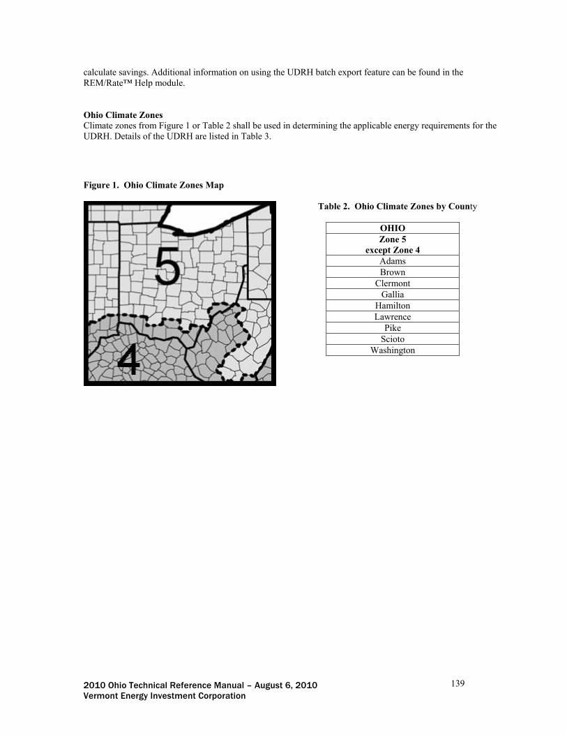
2010 Ohio Technical Reference Manual – August 6, 2010 139 Vermont Energy Investment Corporation
calculate savings. Additional information on using the UDRH batch export feature can be found in the REM/Rate™ Help module. Ohio Climate Zones Climate zones from Figure 1 or Table 2 shall be used in determining the applicable energy requirements for the UDRH. Details of the UDRH are listed in Table 3.
Figure 1. Ohio Climate Zones Map
Table 2. Ohio Climate Zones by County
OHIO Zone 5
except Zone 4 Adams Brown
Clermont Gallia
Hamilton Lawrence
Pike Scioto
Washington

2010 Ohio Technical Reference Manual – August 6, 2010 140 Vermont Energy Investment Corporation
User Defined Reference Home (UDRH) Specifications Table 3 below provides inputs for a UDRH based on the 2006 IECC, with some supplemental clarifications.
Table 3. 2006 IECC UDRH Specifications
Data Point Value Unit Source Comment
Building Thermal Envelope Zone 4 Zone 5 Fenestration 0.40 0.35 U-factor 2006 IECC Table 402.1.3 Skylight 0.60 0.60 U-factor 2006 IECC Table 402.1.3 Glazed Fenestration SHGC 0.40 0.40 SHGC 2006 IECC Table 404.5.2(1) No prescriptive requirement. Ceiling .030 .030 U-factor 2006 IECC Table 402.1.3 Wood Frame Wall .082 .060 U-factor 2006 IECC Table 402.1.3 Rim and Band Joists .082 .060 U-factor Code requirement for wood frame wall. Mass Wall .141 .082 U-factor 2006 IECC Table 402.1.3 Frame Floor .047 .033 U-factor 2006 IECC Table 402.1.3 Basement Wall .059 .059 U-factor 2006 IECC Table 402.1.3 Slab, unheated 10, 2 10, 2 R-value, ft 2006 IECC Table 402.1.1 “ft” = feet from top of slab edge below grade. Slab, heated 15, 2 15, 2 R-value, ft 2006 IECC Table 402.1.1 “ft” = feet from top of slab edge below grade. Crawl Space Wall .065 .065 U-factor 2006 IECC Table 402.1.3 Air Infiltration Rate .00036 .00036 SLA 2006 IECC Table 404.5.2(1) Approximately 7 to 8 ACH50. Mechanical Systems Furnace 80 AFUE Federal Standard Standard is 78 AFUE, 80 AFUE is adopted based on
typical minimum availability and practice. Boiler 80 AFUE Federal Standard Heat Pump, Heating 7.7 HSPF Federal Standard All heat pumps shall be characterized as an ASHP. Central Air Conditioning 13 SEER Federal Standard Heat Pump, Cooling 13 SEER Federal Standard Water Heating, gas 0.58 EF Federal Standard Federal requirements vary based on tank size. The
UDRH feature does not allow adjustments to efficiency values based on tank size, therefore the UDRH reference efficiency shall be based on minimum federal efficiency requirements for a 50 gal tank.
Water Heating, oil 0.50 EF Federal Standard See Water Heating, gas. Water heating, electric 0.90 EF Federal Standard See Water Heating, gas.

2010 Ohio Technical Reference Manual – August 6, 2010 141 Vermont Energy Investment Corporation
Data Point Value Unit Source Comment
Integrated Space/Water Heating, heating
80 AFUE Federal Standard, Boiler Combination space and water heating units shall reference the minimum Federal standard boiler efficiency for the heating portion of the unit
Integrated Space/Water Heating, water
.58 (gas) .50 (oil)
.90 (electric)
EF Federal Standard, Water heating
Combination space and water heating units shall reference the minimum Federal standard water heating efficiency for the water heating portion of the unit.
Thermostat, type Manual 2006 IECC Table 404.5.2(1) Thermostat, cooling set point 78 Degree F 2006 IECC Table 404.5.2(1) Thermostat, heating set point 68 Degree F 2006 IECC Table 404.5.2(1) Duct Insulation 8 R-value 2006 IECC 403.2.1 Duct Insulation, in floor truss 6 R-Value 2006 IECC 403.2.1 Duct Leakage 0.80 DSE 2006 IECC Table 404.5.2(1) Mechanical Ventilation n/a Ventilation is not required by code. The UDRH shall not
reference ventilation. This way the program home will see no energy savings or energy penalty from ventilation.
Lights & Appliances Efficient Lighting 10 Percent RESNET Standard Refrigerator 585 kWh/yr VEIC Based on the weighted average of NAECA baseline
kWh/yr installed in Vermont, 5000 hr/yr. Dishwasher 0.46 EF RESNET Standard Ceiling Fan None RESNET Standard Active Solar & Photovoltaics (PV) Solar systems installed for water and/or space heating and photovoltaic systems installed to meet electricity demand are not addressed in the 2006 IECC. However, they need to be addressed in the UDRH. If the RNC program allows for savings to be claimed from the use of active solar or PV systems, these systems should eliminated from the UDRH so that their savings shows up when compared to the rated home with the solar system installed. If the RNC program does not allow savings to be claimed from the use of active solar or PV systems, these systems should not be included in the UDRH. When a system is not referenced in the UDRH, that system will be the same in both the Rated and the Reference home. This way, energy consumption for the Rated Home and the UDRH will be estimated assuming both configurations have the solar or PV system installed, so no savings will be reported. The specific syntax for this is provided in the REM/Rate™ UDRH Syntax Report.

2010 Ohio Technical Reference Manual – August 6, 2010 142 Vermont Energy Investment Corporation
Other Software If the program implementer is using a RESNET approved software program other than REM/Rate™, where possible a module similar to the UDRH feature in REM/Rate™ shall be used to estimate energy and demand savings. If no such feature exists, the following steps shall be taken to estimate energy and demand savings:
1. Model the home in a RESNET approved software program and capture energy consumption and electric demand.
2. Model the same home a second time using the 2006 UDRH specifications provided in Table 3 and capture energy consumption and electric demand.
3. The difference between energy consumption in the Rated Home and the Rated Home modeled to 2006 IECC specifications shall be the energy savings for that home.
4. The difference between electric demand in the Rated Home and the Rated Home modeled to 2006 IECC specifications shall be the electric demand savings for that home.
Savings from lighting and appliances shall be estimated using the alternate RESNET approved software. Any appliances not captured by the alternate software program shall be captured by a program other than RNC. Deemed Lifetime of Efficient Building 25 yr (for heating, cooling, and shell savings measures)346 Deemed Measure Cost Incremental costs can be calculated for different tiers of efficient homes from the following table. Table 4. Incremental Costs from Baseline to Specific HERS Levels347 ENERGY STAR
Minimum (HERS 85)*
HERS 70
HERS 65
Single Family Home with Gas Furnace total and per square foot cost
$2,869 $1.18
$7,136 $2.94
$9,286 $3.83
Single Family Home with Gas Boiler total and per square foot cost
$2,646 $1.09
$6,570 $2.71
$8,160 $3.36
Single Family Home with Oil Boiler total and per square foot cost
$2,371 $0.98
$6,325 $2.61
$7,914 $3.26
Average for all single family total and per square foot cost
$2,599 $1.07
$6,677 $2.75
$8,453 $3.49
*Calculated as an average of the packages provided for each housing type/HVAC system combination Deemed O&M Cost Adjustments There are no operation and maintenance cost adjustments for this measure Fossil Fuel Impact Descriptions and Calculation Energy savings, including fossil fuel savings, for heating, cooling, hot water, lighting, and appliances noted above will be a direct output of REM/Rate™ (or other RESNET approved) energy modeling software as described above Water Impact Descriptions and Calculation n/a
346 Measure Life Report, Residential and Commercial/Industrial Lighting and HVAC Measures, GDS Associates, June 2007; http://www.ctsavesenergy.org/files/Measure%20Life%20Report%202007.pdf 347 Evaluation of the Massachusetts New Homes with Energy Star® Program, Incremental Cost Analysis Nexus Market Research, Inc. and Dorothy Conant, Nov. 2007

2010 Ohio Technical Reference Manual – August 6, 2010 143 Vermont Energy Investment Corporation
Version Date & Revision History Draft: Portfolio # Effective date: Date TRM will become effective End date: Date TRM will cease to be effective (or TBD)

2010 Ohio Technical Reference Manual – August 6, 2010 144 Vermont Energy Investment Corporation
Whole-House Residential Retrofit Official Measure Code (Measure Number: X-X-X-X (Program name, End Use) Description Whole house retrofit programs, like Home Performance with ENERGY STAR and Low Income Weatherization initiatives, may include a variety of treatments, including building shell and HVAC upgrades and the direct installation of energy efficient products. This protocol describes how building energy modeling of each individual home treated through a program may be used to estimate savings for the building shell (e.g., air-sealing and insulation) and HVAC (e.g., duct sealing and central heating and/or cooling system replacements) measures installed in those homes. Savings from other measures such as efficient lighting, appliances, or water heating should be estimated using deemed values or deemed calculations provided for such measures elsewhere in this TRM. The alternative to using building energy modeling to develop energy savings for the shell and HVAC measures would be to use the deemed measure savings calculations found elsewhere in this TRM for the installed measures (air-sealing, insulation, duct sealing, etc.). Deemed savings calculations are simpler to administer and implement but may be less precise because they are based on some assumed average characteristics of homes (e.g., average heating system efficiencies) and do not capture interactive effects between some measures. Definition of Efficient Case House as treated by installed building shell and HVAC measures. Installed measures outside of these categories should follow the appropriate measure-specific characterizations. Definition of Baseline Case The baseline is the house as it is before it is retrofitted with installed measures. The only exception to this rule is that the assumed baseline efficiency of a heating system or central air conditioner that is being replaced should be consistent with the current minimum federal efficiency standards for such equipment, unless it is clear that the equipment would not have been replaced at that particular point in time were it not for the influence of the program (i.e., the program must document that old equipment would otherwise not have been replaced in order to claim a baseline efficiency that is lower than current minimum federal efficiency standards). Calculation of Savings The requirements for a model-based approach to savings claims are in part are delineated through adherence with at least one of the following national standards for whole-house savings calculations:
RESNET348 approved rating software Software energy simulation performance exceeding the requirements of National Renewable
Energy Laboratory’s Home Energy Rating System BESTEST349 US DOE Weatherization Assistance Program approval350
Proper savings estimates from modeling software also require that the R-value of uninsulated walls or ceilings (i.e., baseline conditions) should be modeled as being no less than R-5. In addition, software tools must be calibrated against actual consumption data for each treated home or from a sample sized for 90% confidence interval and 10% margin of error statistical precision. These requirements address concerns that modeling software can over-estimates savings, particularly cooling savings. The software tools must provide outputs that separately account for heating and cooling energy savings so
348 http://resnet.us 349 http://www.nrel.gov/docs/legosti/fy96/7332b.pdf 350 http://www.waptec.org

2010 Ohio Technical Reference Manual – August 6, 2010 145 Vermont Energy Investment Corporation
that demand and fuel-related economic savings may be properly addressed. Summer Coincident Peak Demand Savings Cooling only: ΔkW = ΔkWhCOOL / FLHCOOL *CF where:
FLHCOOL = Full load cooling hours, dependent on location as below:
Location Run Hours351 Akron 476
Cincinnati 664 Cleveland 426 Columbus 552
Dayton 631 Mansfield 474
Toledo 433 Youngstown 369
CF = Summer Peak Coincidence Factor for measure
= 0.5352 For example if the cooling savings output from the software tool for a home in Toledo is 350kWh then: ΔkW = ΔkWh / FLHcool *CF = 350 / 433* 0.5 = 0.404 kW Deemed Lifetime of Efficient Case The average savings-weighted lifetime for this measure is assumed to be 20 years, based upon an anticipated mixture of shell and HVAC measures that range from 15 to 25 years.353 Deemed Measure Cost The total of the actual costs in procuring and installing the equipment, materials, and/or services Deemed O&M Cost Adjustments n/a Version Date & Revision History Draft: Portfolio # Effective date: Date TRM will become effective End date: Date TRM will cease to be effective (or TBD)
351 Based on Full Load Hour assumptions taken from the ENERGY STAR calculator (http://www.energystar.gov/ia/business/bulk_purchasing/bpsavings_calc/Calc_CAC.xls) and reduced by 33% due to assumption that the average air conditioning is oversized by 50% (Neme, Proctor, Nadal, 1999; “National Energy Savings Potential From Addressing Residential HVAC Installation Problems”). Note this approach results in full load hour estimates within 10% of measured estimates from the Energy Center of Wisconsin, May 2008 study; “Central Air Conditioning in Wisconsin, A Compilation of Recent Field Research.” 352 Based on Energy Center of Wisconsin, May 2008 metering study; “Central Air Conditioning in Wisconsin, A Compilation of Recent Field Research”, p32 353 A review of actual measures installed through the program should be conducted to assess whether on a savings basis the weighted average should be adjusted in accordance with a measure distribution that favors longer (insulation) or shorter (air sealing) lifetimes.

2010 Ohio Technical Reference Manual – August 6, 2010 146 Vermont Energy Investment Corporation
III. Commercial & Industrial Market Sector
Electric Chiller (Time of Sale) Official Measure Code (Measure Number: X-X-X-X (Program name, End Use) Description This measure relates to the installation of a new electric chiller meeting the efficiency standards presented below. This measure could relate to the replacement of an existing unit at the end of its useful life, or the installation of a new system in an existing building (i.e. time of sale). Only single-chiller applications should be assessed with this methodology. The characterization is not suited for multiple chillers projects or chillers equipped with variable speed drives (VSDs). Multiple chiller projects and chillers equipped with VSDs should be evaluated on a custom basis. Definition of Efficient Equipment In order for this characterization to apply, the efficient equipment is assumed to exceed the efficiency requirements of the 2006 International Energy Conservation Code, Table 503.2.3(7). Definition of Baseline Equipment In order for this characterization to apply, the baseline equipment is assumed to meet the efficiency requirements of the 2006 International Energy Conservation Code, Table 503.2.3(7). Deemed Calculation for this Measure
Annual kWh Savings = TONS * ((3.516/IPLVbase) – (3.516/IPLVee)) * EFLH Summer Coincident Peak kW Savings = TONS * ((3.516/COPbase) – (3.516/COPee)) * CF
Deemed Lifetime of Efficient Equipment The expected measure life is assumed to be 20 years 354. Deemed Measure Cost The incremental capital cost for this measure is provided below.
Equipment Type Size Category Incremental Cost ($/ton)355 Air cooled, electrically operated All capacities $127/ton356 Water cooled, electrically operated, positive displacement (reciprocating)
All capacities $22/ton
< 150 tons $128/ton >= 150 tons and < 300 tons
$70/ton Water cooled, electrically operated, positive displacement (rotary screw and scroll)
>= 300 tons $48/ton
354 2008 Database for Energy-Efficiency Resources (DEER), Version 2008.2.05, “Effective/Remaining Useful Life Values”, California Public Utilities Commission, December 16, 2008 (http://deeresources.com/deer0911planning/downloads/EUL_Summary_10-1-08.xls) 355 2008 Database for Energy-Efficiency Resources (DEER), Version 2008.2.05, “Cost Values and Summary Documentation”, California Public Utilities Commission, December 16, 2008 (http://deeresources.com/deer0911planning/downloads/DEER2008_Costs_ValuesAndDocumentation_080530Rev1.zip) 356 Calculated as the simple average of screw and reciprocating air-cooled chiller incremental costs from the reference noted in Footnote 355.

2010 Ohio Technical Reference Manual – August 6, 2010 147 Vermont Energy Investment Corporation
Equipment Type Size Category Incremental Cost ($/ton)355 Water cooled, electrically operated, centrifugal
All capacities $177/ton357
Deemed O&M Cost Adjustments n/a Coincidence Factor The summer peak coincidence factor for this measure is assumed to be 74%358.
REFERENCE SECTION
Calculation of Savings Energy Savings
ΔkWH = TONS * ((3.516/IPLVbase) – (3.516/IPLVee)) * EFLH
Where: TONS = chiller nominal cooling capacity in tons (note: 1 ton = 12,000 Btu/h) = Actual installed 3.516 = conversion factor to express Integrated Part Load Value (IPLV) in terms of
kW per ton IPLVbase = efficiency of baseline equipment expressed as Integrated Part Load Value.
Dependent on chiller type. See Table A in the Reference Tables section. IPLVee359 = efficiency of high efficiency equipment expressed as Integrated Part Load
Value = Actual installed
EFLH = equivalent full load hours Dependent on location as below:
EFLH by Location360 System Type Akron Columbus Cincinnati Cleveland Dayton Mansfield Toledo CV reheat, no economizer 2,866 2,633 2,940 2,762 3,063 2,960 2,743 CV reheat, economizer 793 941 955 932 976 921 859 VAV reheat, economizer 788 946 974 768 896 669 848
Summer Coincident Peak Demand Savings
ΔkW = TONS * ((3.516/COPbase) – (3.516/COPee)) * CF
Where:
COPbase = efficiency of baseline equipment expressed as COP 357 Calculated as the simple average of non-VSD water-cooled centrifugal chiller incremental costs from the reference noted in Footnote 355. 358 Summer Peak Coincidence Factor has been preserved from the “Technical Reference Manual (TRM) for Ohio Senate Bill 221 Energy Efficiency and Conservation Program and 09-512-GE-UNC”, October 15, 2009. This is likely a conservative estimate, but is recommended for further study. 359 Integrated Part Load Value is simply a seasonal average efficiency rating calculated in accordance with ARI Standard 550/590. It may be calculated using any measure of efficiency (EER, kW/ton, COP), but for consistency with IECC 2006, it is expressed in terms of COP here. 360 Cooling EFLHs have been preserved from the “Technical Reference Manual (TRM) for Ohio Senate Bill 221 Energy Efficiency and Conservation Program and 09-512-GE-UNC”, October 15, 2009. These appear reasonable, but are recommended for further study.

2010 Ohio Technical Reference Manual – August 6, 2010 148 Vermont Energy Investment Corporation
Dependent on chiller type. See Table A in the Reference Tables section.
COPee = efficiency of high efficiency equipment expressed as COP = Actual installed
CF = Summer Peak Coincidence Factor for measure = 74%
Fossil Fuel Impact Descriptions and Calculation n/a Water Impact Descriptions and Calculation n/a Deemed O&M Cost Adjustment Calculation n/a Reference Tables Table A: Baseline Efficiency Values by Chiller Type and Capacity361
Equipment Type Size Category Baseline Efficiency
(IPLVbase, COPbase) < 150 tons 2.80 IPLV, 2.80 COP Air cooled, with condenser,
electrically operated >= 150 tons 2.50 IPLV, 2.50 COP
Air cooled, without condenser, electrically operated All capacities 3.10 IPLV, 3.10 COP
Water cooled, electrically operated, positive displacement (reciprocating) All capacities 4.65 IPLV, 4.20 COP
< 150 tons 4.50 IPLV, 4.45 COP
>= 150 tons and < 300 tons 4.95 IPLV, 4.90 COP
Water cooled, electrically operated, positive displacement (rotary screw and scroll) >= 300 tons 5.60 IPLV, 5.50 COP
< 150 tons 5.00 IPLV, 5.00 COP
>= 150 tons and < 300 tons 5.55 IPLV, 5.55 COP Water cooled, electrically
operated, centrifugal >= 300 tons 6.10 IPLV, 6.10 COP Version Date & Revision History Draft: Portfolio # Effective date: Date TRM will become effective End date: TBD
361 2006 International Energy Conservation Code, International Code Council, Inc., January 2006.

2010 Ohio Technical Reference Manual – August 6, 2010 149 Vermont Energy Investment Corporation
C&I Lighting Controls (Time of Sale, Retrofit) Official Measure Code (Measure Number: X-X-X-X (Program name, End Use) Description This measure relates to the installation of a new lighting control on a new or existing lighting system. Lighting control types covered by this measure include wall- or ceiling-mounted occupancy sensors, fixture mounted occupancy sensors, remote-mounted daylight dimming sensors, fixture mounted daylight dimming sensors, central lighting controls (timeclocks), and switching controls for multi-level lighting. This measure could relate to the installation of a new system in an existing building or a new construction application (i.e., time of sale). Lighting controls required by state energy codes are not eligible. Definition of Efficient Equipment In order for this characterization to apply, the efficient equipment is assumed to be a lighting system controlled by one of the lighting controls systems listed above. Definition of Baseline Equipment The baseline equipment is assumed to be an uncontrolled lighting systems operated by a manual switch. Deemed Calculation for this Measure
Annual kWh Savings = kWcontrolled * HOURS * (1 + IFkWh) * ESF Summer Coincident Peak kW Savings = kWcontrolled * (1 + IFkW) * ESF * CF
Deemed Lifetime of Efficient Equipment The expected measure life for all lighting controls is assumed to be 8 years 362. Deemed Measure Cost The incremental capital cost for this measure is provided below.
Lighting Control Type Incremental Cost Wall-Mounted Occupancy Sensors $42363 Ceiling-Mounted Occupancy Sensors $66364 Fixture Mounted Occupancy Sensors $125365 Remote-Mounted Daylight Dimming Sensors $65366 Fixture Mounted Daylight Dimming Sensors $50367 Switching Controls for Multi-Level Lighting $274368 Central Lighting Controls (Timeclocks) $103369
362 2008 Database for Energy-Efficiency Resources (DEER), Version 2008.2.05, “Effective/Remaining Useful Life Values”, California Public Utilities Commission, December 16, 2008 (http://deeresources.com/deer0911planning/downloads/EUL_Summary_10-1-08.xls) 363 Goldberg et al, State of Wisconsin Public Service Commission of Wisconsin, Focus on Energy Evaluation, Business Programs: Incremental Cost Study, KEMA, October 28, 2009. 364 Ibid. 365 Efficiency Vermont Technical Reference User Manual (TRM) Measure Savings Algorithms and Cost Assumptions, February, 19, 2010. 366 Ibid. 367 Ibid. 368 Goldberg et al, State of Wisconsin Public Service Commission of Wisconsin, Focus on Energy Evaluation, Business Programs: Incremental Cost Study, KEMA, October 28, 2009. 369 2008 Database for Energy-Efficiency Resources (DEER), Version 2008.2.05, “Cost Values and Summary Documentation”, California Public Utilities Commission, December 16, 2008

2010 Ohio Technical Reference Manual – August 6, 2010 150 Vermont Energy Investment Corporation
Deemed O&M Cost Adjustments n/a Coincidence Factor The summer peak coincidence factor for this measure is dependent on technology type as below: Lighting Control Type CF Wall- or Ceiling-Mounted Occupancy Sensors 0.15370 Fixture-Mounted Occupancy Sensors 0.15371 Remote-Mounted Daylight Dimming Sensors 0.90372 Fixture-Mounted Daylight Dimming Sensors 0.90373 Switching Controls for Multi-Level Lighting 0.77374 Central Lighting Controls (Timeclocks) 0.00375
REFERENCE SECTION
Calculation of Savings Energy Savings
ΔkWh = kWcontrolled * HOURS * (1 + IFkWh) * ESF
Where: kWcontrolled = total lighting load connected to the control in kilowatts = Actual installed HOURS = total operating hours of the controlled lighting before the lighting controls are
installed. If actual site-specific value is unknown, assume default values dependent on building type as below:
Building Type HOURS376 Food Sales 5,544 Food Service 4,482 Health Care 3,677 Hotel/Motel 3,356 Office 3,526 Public Assembly 2,729 Public Services (non-food) 3,425 Retail 4,226 Warehouse 3,464 School 2,302
(http://deeresources.com/deer0911planning/downloads/DEER2008_Costs_ValuesAndDocumentation_080530Rev1.zip) 370 Coincidence Factor Study Residential and Commercial Industrial Lighting Measures, RLW Analytics, Spring 2007. 371 Ibid. 372 Kuiken et al, Focus on Energy Evaluation, Business Programs: Deemed Savings Manual V1.0, KEMA, March 22, 2010. 373 Ibid. 374 Ibid. 375 Conservative assumption based on professional judgment considering that timeclocks are unlikely to produce significant savings during the summer on-peak period. 376 Kuiken et al, “State of Wisconsin Public Service Commission of Wisconsin Focus on Energy Evaluation Business Programs: Deemed Savings Parameter Development”, KEMA, November 13, 2009, unless otherwise noted.

2010 Ohio Technical Reference Manual – August 6, 2010 151 Vermont Energy Investment Corporation
Building Type HOURS376 College 3,900 Industrial – 1 Shift 2,857377 Industrial – 2 Shift 4,730378 Industrial – 3 Shift 6,631379 Exterior 3,833380 Other 3,672
IFkWh = lighting-HVAC Interation Factor for energy; this factor represents the reduced
electric space cooling requirements due to the reduction on waste heat rejected by the efficent lighting.
= 0.095 (interior fixtures), 0.000 (exterior fixtures)381 ESF = Energy Savings Factor; percent operating hours reduced due to the installation
of the occupancy lighting controls or timeclocks, or percent wattage reduction multiplied by the hours of dimming for dimming lighting controls and multilevel switching.
Dependent on control type as below:
Lighting Control Type ESF382 Wall- or Ceiling-Mounted Occupancy Sensors 30% Fixture-Mounted Occupancy Sensors 30% Remote-Mounted Daylight Dimming Sensors 30% Fixture-Mounted Daylight Dimming Sensors 30% Switching Controls for Multi-Level Lighting 30% Central Lighting Controls (Timeclocks) 10%
Summer Coincident Peak Demand Savings
ΔkW = kWconnected * (1 + IFkW) * ESF * CF
Where: IFkW = lighting-HVAC Interation Factor for demand; this factor represents the
reduced electric space cooling requirements due to the reduction on waste heat rejected by the efficent lighting. = 0.200 (interior fixtures), 0.000 (exterior fixtures) 383
377 UI and CL&P Program Savings Documentation for 2010 Program Year, United Illuminating Company, September 2009. 378 Ibid. 379 Ibid. 380 Exterior lighting 3,833 hours per year assumes 10.5 hours per day; typical average for photocell control. 381 Interactive factor data based on a series of prototypical small commercial building simulation runs. Values shown are weighted averages across fast food restaurant, full service restaurant, assembly, big box retail, small retail, small office, light industrial and school building models. The prototypes are based on the California DEER study prototypes, modified for local construction practices. Simulations were run using TMY3 weather data for the following Ohio cities: Cincinnati, Cleveland, Columbus and Dayton. Building prototypes used in the energy modeling are described in Appendix A - Prototypical Building Energy Simulation Model Development. 382 Energy Savings Factors determined from a review of Efficiency Vermont Technical Reference User Manual (TRM) Measure Savings Algorithms and Cost Assumptions, February, 19, 2010, New York Standard Approach for Estimating Energy Savings from Energy Efficiency Measures in Commercial and Industrial Programs, TecMarket Works, September 1, 2009, Goldberg et al, State of Wisconsin Public Service Commission of Wisconsin, Kuiken et al, Focus on Energy Evaluation, Business Programs: Deemed Savings Manual V1.0, KEMA, March 22, 2010. 383 Interactive factor data based on a series of prototypical small commercial building simulation runs. Values shown are weighted averages across fast food restaurant, full service restaurant, assembly, big box retail, small retail, small office, light industrial and school building models. The prototypes are based on the California DEER study prototypes, modified for local construction practices. Simulations were run using TMY3 weather data for the following Ohio

2010 Ohio Technical Reference Manual – August 6, 2010 152 Vermont Energy Investment Corporation
CF = Summer Peak Coincidence Factor for measure Dependent on control type as presented in the introductory “Coincidence Factor” section.
Fossil Fuel Impact Descriptions and Calculation
ΔMMBtu = ΔkWh * IFMMBtu
Where: IFMMBtu = lighting-HVAC Interation Factor for gas heating impacts; this factor
represents the increased gas space heating requirements due to the reduction of waste heat rejected by the efficent lighting. = -0.0028 (interior fixtures), 0.0000 (exterior fixtures) 384
Water Impact Descriptions and Calculation n/a Deemed O&M Cost Adjustment Calculation n/a Version Date & Revision History Draft: Portfolio # Effective date: Date TRM will become effective End date: Date TRM will cease to be effective (or TBD)
cities: Cincinnati, Cleveland, Columbus and Dayton. Building prototypes used in the energy modeling are described in Appendix A - Prototypical Building Energy Simulation Model Development. 384 Ibid.

2010 Ohio Technical Reference Manual – August 6, 2010 153 Vermont Energy Investment Corporation
Lighting Systems (Non-Controls) (Time of Sale, New Construction) Official Measure Code (Measure Number: X-X-X-X (Program name, End Use) Description This measure relates to the installation of new lighting equipment with efficiency that exceeds that of equipment that would have been installed following standard market practices. This characterization includes compact fluorescent lamps (CFLs) and fixtures, linear fluorescent lamps and fixtures, linear fluorescent fixtures replacing high-intensity discharge (HID) fixtures in high-bay applications, and high-intensity discharge (HID) fixtures. This measure could relate to the replacement of an existing unit at the end of its useful life or the installation of a new unit in a new or existing facility. Definition of Efficient Equipment In order for this characterization to apply, the efficient equipment must have higher efficiency than the existing equipment and meet program specific equipment criteria. Definition of Baseline Equipment The assumed baseline equipment varies by technology type.
Compact Fluorescent Lamps Deemed Calculation for Compact Fluorescent Lamps This measure relates to the installation of a new ENERGY STAR certified compact fluorescent screw-in lamp (CFL) (for those equipment types for which an ENERGY STAR category exists). This measure could relate to the replacing of an existing unit at the end of its useful life, or the installation of a new unit in a new or existing building (i.e. time of sale). This measure applies to the installation of a screw-in CFL replacing a standard general service incandescent lamp.
Annual kWh Savings385 = (WATTSee * 2.79) * HOURS * (1 + WHFe) / 1000 Summer Coincident Peak kW Savings = (WATTSee * 2.79) * CF * (1 + WHFd) / 1000
Note: The multiplier should be adjusted according to the table below to account for the change in
baseline stemming from the Energy Independence and Security Act of 2007 discussed below:
Delta Watts Multiplier386 CFL Wattage
2009 - 2011 2012 2013 2014 and Beyond
15 or less 2.79 2.79 2.79 1.72
16-20 2.79 2.79 1.68 1.68
21W+ 2.79 1.73 1.73 1.73
Baseline Adjustment for Compact Fluorescent Lamps 385 Kuiken et al, Focus on Energy Evaluation, Business Programs: Deemed Savings Manual V1.0, KEMA, March 22, 2010. Source document cites several evaluations indicating that the overall average existing incandescent lamp wattage is 75.7W and the overall average replacement wattage is 20.0W for CFLs <= 32W. For the purposes of this characterization, it is assumed that the baseline and efficient wattages are directly proportional. These assumptions have been simplified as follows: (WATTSbase – WATTSee) = [(75.7/20.0)* WATTSee] – WATTSee = WATTSee * 2.79. 386 Calculated by finding the new delta watts after incandescent bulb wattage reduced (from 100W to 72W in 2012, 75W to 53W in 2013 and 60W to 43W in 2014).
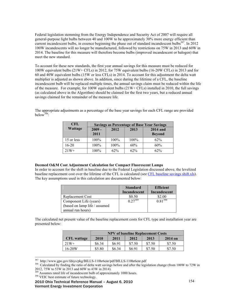
2010 Ohio Technical Reference Manual – August 6, 2010 154 Vermont Energy Investment Corporation
Federal legislation stemming from the Energy Independence and Security Act of 2007 will require all general-purpose light bulbs between 40 and 100W to be approximately 30% more energy efficient than current incandescent bulbs, in essence beginning the phase out of standard incandescent bulbs387. In 2012 100W incandescents will no longer be manufactured, followed by restrictions on 75W in 2013 and 60W in 2014. The baseline for this measure will therefore become bulbs (improved incandescent or halogen) that meet the new standard. To account for these new standards, the first year annual savings for this measure must be reduced for 100W equivalent bulbs (21W+ CFLs) in 2012, for 75W equivalent bulbs (16-20W CFLs) in 2013 and for 60 and 40W equivalent bulbs (15W or less CFLs) in 2014. To account for this adjustment the delta watt multiplier is adjusted as shown above. In addition, since during the lifetime of a CFL, the baseline incandescent bulb will be replaced multiple times, the annual savings claim must be reduced within the life of the measure. For example, for 100W equivalent bulbs (21W+ CFLs) installed in 2010, the full savings (as calculated above in the Algorithm) should be claimed for the first two years, but a reduced annual savings claimed for the remainder of the measure life. The appropriate adjustments as a percentage of the base year savings for each CFL range are provided below388:
Savings as Percentage of Base Year Savings CFL Wattage 2009 -
2011 2012 2013 2014 and
Beyond
15 or less 100% 100% 100% 62%
16-20 100% 100% 60% 60%
21W+ 100% 62% 62% 62%
Deemed O&M Cost Adjustment Calculation for Compact Fluorescent Lamps In order to account for the shift in baseline due to the Federal Legislation discussed above, the levelized baseline replacement cost over the lifetime of the CFL is calculated (see CFL baseline savings shift.xls). The key assumptions used in this calculation are documented below:
Standard Incandescent
Efficient Incandescent
Replacement Cost $0.50 $2.00 Component Life (years) (based on lamp life / assumed annual run hours)
0.27389 0.81390
The calculated net present value of the baseline replacement costs for CFL type and installation year are presented below:
NPV of baseline Replacement Costs CFL wattage 2010 2011 2012 2013 2014 on
21W+ $6.34 $6.91 $7.50 $7.50 $7.50 16-20W $5.80 $6.34 $6.91 $7.50 $7.50
387 http://www.gpo.gov/fdsys/pkg/BILLS-110hr6enr/pdf/BILLS-110hr6enr.pdf 388 Calculated by finding the ratio of delta watt savings before and after the legislation change (from 100W to 72W in 2012, 75W to 53W in 2013 and 60W to 43W in 2014). 389 Assumes rated life of incandescent bulb of approximately 1000 hours. 390 VEIC best estimate of future technology.
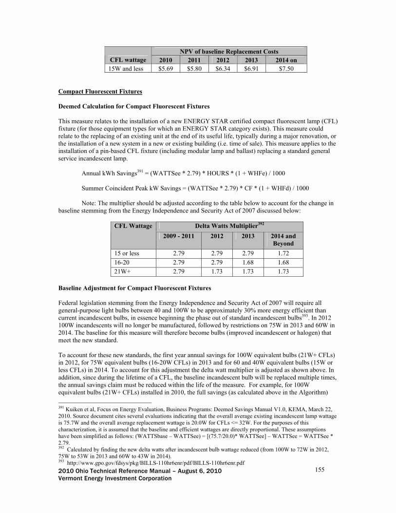
2010 Ohio Technical Reference Manual – August 6, 2010 155 Vermont Energy Investment Corporation
NPV of baseline Replacement Costs CFL wattage 2010 2011 2012 2013 2014 on
15W and less $5.69 $5.80 $6.34 $6.91 $7.50 Compact Fluorescent Fixtures Deemed Calculation for Compact Fluorescent Fixtures
This measure relates to the installation of a new ENERGY STAR certified compact fluorescent lamp (CFL) fixture (for those equipment types for which an ENERGY STAR category exists). This measure could relate to the replacing of an existing unit at the end of its useful life, typically during a major renovation, or the installation of a new system in a new or existing building (i.e. time of sale). This measure applies to the installation of a pin-based CFL fixture (including modular lamp and ballast) replacing a standard general service incandescent lamp.
Annual kWh Savings391 = (WATTSee * 2.79) * HOURS * (1 + WHFe) / 1000 Summer Coincident Peak kW Savings = (WATTSee * 2.79) * CF * (1 + WHFd) / 1000 Note: The multiplier should be adjusted according to the table below to account for the change in
baseline stemming from the Energy Independence and Security Act of 2007 discussed below:
Delta Watts Multiplier392 CFL Wattage
2009 - 2011 2012 2013 2014 and Beyond
15 or less 2.79 2.79 2.79 1.72
16-20 2.79 2.79 1.68 1.68
21W+ 2.79 1.73 1.73 1.73
Baseline Adjustment for Compact Fluorescent Fixtures Federal legislation stemming from the Energy Independence and Security Act of 2007 will require all general-purpose light bulbs between 40 and 100W to be approximately 30% more energy efficient than current incandescent bulbs, in essence beginning the phase out of standard incandescent bulbs393. In 2012 100W incandescents will no longer be manufactured, followed by restrictions on 75W in 2013 and 60W in 2014. The baseline for this measure will therefore become bulbs (improved incandescent or halogen) that meet the new standard. To account for these new standards, the first year annual savings for 100W equivalent bulbs (21W+ CFLs) in 2012, for 75W equivalent bulbs (16-20W CFLs) in 2013 and for 60 and 40W equivalent bulbs (15W or less CFLs) in 2014. To account for this adjustment the delta watt multiplier is adjusted as shown above. In addition, since during the lifetime of a CFL, the baseline incandescent bulb will be replaced multiple times, the annual savings claim must be reduced within the life of the measure. For example, for 100W equivalent bulbs (21W+ CFLs) installed in 2010, the full savings (as calculated above in the Algorithm)
391 Kuiken et al, Focus on Energy Evaluation, Business Programs: Deemed Savings Manual V1.0, KEMA, March 22, 2010. Source document cites several evaluations indicating that the overall average existing incandescent lamp wattage is 75.7W and the overall average replacement wattage is 20.0W for CFLs <= 32W. For the purposes of this characterization, it is assumed that the baseline and efficient wattages are directly proportional. These assumptions have been simplified as follows: (WATTSbase – WATTSee) = [(75.7/20.0)* WATTSee] – WATTSee = WATTSee * 2.79. 392 Calculated by finding the new delta watts after incandescent bulb wattage reduced (from 100W to 72W in 2012, 75W to 53W in 2013 and 60W to 43W in 2014). 393 http://www.gpo.gov/fdsys/pkg/BILLS-110hr6enr/pdf/BILLS-110hr6enr.pdf

2010 Ohio Technical Reference Manual – August 6, 2010 156 Vermont Energy Investment Corporation
should be claimed for the first two years, but a reduced annual savings claimed for the remainder of the measure life. . The appropriate adjustments as a percentage of the base year savings for each CFL range are provided below394:
Savings as Percentage of Base Year Savings CFL Wattage 2009 -
2011 2012 2013 2014 and
Beyond
15 or less 100% 100% 100% 62%
16-20 100% 100% 60% 60%
21W+ 100% 62% 62% 62%
Deemed O&M Cost Adjustment Calculation for Compact Fluorescent Fixtures Conservatively not included High Bay Fluorescent Fixtures Deemed Calculation for High Bay Fluorescent Fixtures The assumed baseline for installation of a high bay fluorescent fixture is a metal halide system. The Energy Independence and Security Act of 2007 (EISA) requires that as of January 1, 2009, metal halide fixtures designed for use with lamps ≥150 W and ≤500 W must use “probe start” ballasts with ballast efficiency ≥94% or “pulse start” ballasts with ballast efficiency ≥88. It is therefore likely that new metal halide fixtures will utilize “pulse start” technology. Therefore, the assumed baseline system is a magnetic ballast “pulse start” metal halide system.
Annual kWh Savings = (WATTSbase – WATTSee) * HOURS * (1 + WHFe) / 1000 Summer Coincident Peak kW Savings = (WATTSbase – WATTSee) * CF * (1 + WHFd) / 1000
See
394 Calculated by finding the ratio of delta watt savings before and after the legislation change (from 100W to 72W in 2012, 75W to 53W in 2013 and 60W to 43W in 2014).

2010 Ohio Technical Reference Manual – August 6, 2010 157 Vermont Energy Investment Corporation
Table 4 for WATTSbase and WATTSee values. Deemed O&M Cost Adjustment Calculation for High Bay Fluorescent Fixtures O&M cost adjustments were developed assuming a typical baseline system and two typical efficient equipment scenarios. For T5HO High Bay fixtures replacing pulse start metal halide fixtures, the levelized annual baseline replacement cost assumption is calculated as $5.87. For T8VHO high bay fixtures replacing pulse start metal halide fixtures, the levelized annual baseline replacement cost assumption is calculated as -$1.69. The assumptions used to calculate these adjustments are detailed below. Baseline 320W Metal-Halide Lamp Cost: $25.00 Baseline 320W Lamp Life: 15,000 hrs Baseline Lamp Labor Cost: $5.00 (15 min @ $20 per hour labor) Baseline 320W Ballast Cost: $60.00 Baseline Ballast Life: 40,000 Baseline Ballast Labor Cost: $22.50 (30 min @ $45 per hour labor) T5 High-Bay Lamp Cost: $5 per lamp (assumes 4 lamps fixture) T5 High-Bay Lamp Life: 20,000 hrs T5 High-Bay Lamp Labor Cost: $6.67 (20 min @ $20 per hour labor) T5 High-Bay Ballast Cost: $51.00 T5 High-Bay Ballast Life: 70,000 hrs T5 High-Bay Ballast Labor Cost: $22.50 (30 min @ $45 per hour labor) T8 High-Bay Lamp Cost: $10 per lamp (assumes 6 lamp fixture) T8 High-Bay Lamp Life: 18,000 hrs T8 High-Bay Lamp Labor Cost: $13.33 (40 min @ $20 per hour labor) T8 High-Bay Ballast Cost: $100.00 (2 ballasts) T8 High-Bay Ballast Life: 70,000 hrs T8 High-Bay Ballast Labor Cost: $45 (60 min @ $45 per hour labor)

2010 Ohio Technical Reference Manual – August 6, 2010 158 Vermont Energy Investment Corporation
High Efficiency Linear Fluorescent Fixtures Deemed Calculation for High Efficiency Fluorescent Fixtures The assumed baseline for installation of a fluorescent fixture varies by the efficient system installed. High Performance and Reduced Wattage T8s must comply with the requirements as published by the Consortium for Energy Efficiency395.
Annual kWh Savings = (WATTSbase – WATTSee) * HOURS * (1 + WHFe) / 1000 Summer Coincident Peak kW Savings = (WATTSbase – WATTSee) * CF * (1 + WHFd) / 1000
See Table 5 for WATTSbase and WATTSee values. Baseline Adjustment The U.S. Department of Energy issued on June 26, 2009 a final rule, amending the energy conservation standards for general service fluorescent lamps.396 The standards established in the final rule will be applied starting July 14, 2012. These standards essentially require that certain linear fluorescent lamp types meet High Performance T8 specifications..397 For some equipment types, baseline lamps will become unavailable and participants will be required to upgrade both lamps and ballasts to High Performance T8s, thus negating any savings. Assuming a typical lamp has a lifetime of 18,000 hours and is operated 3,730 hours per year, new lamps installed shortly before the impending federal standards take effect will need to be replaced in mid-2017, indicating that savings should be claimed for only 7 years for measures installed in 2010. This baseline adjustment has been incorporated into the measure life for the applicable equipment types. Deemed O&M Cost Adjustment Calculation Conservatively not included Metal Halide Track Lighting Deemed Calculation for Metal Halide Track Lighting
A metal-halide track head produces equal or more light as compared to halogen track head(s), while using fewer watts. This measure applies to the installation of a metal halide track head replacing (a) halogen track head(s).
Annual kWh Savings = (WATTSbase – WATTSee) * HOURS * (1 + WHFe) / 1000 Summer Coincident Peak kW Savings = (WATTSbase – WATTSee) * CF * (1 + WHFd) / 1000
395 The Consortium for Energy Efficiency publishes the High Performance T8 Specifications and the Reduced Wattage T8 Specifications periodically including a list of qualifying equipment at the following address: http://www.cee1.org/com/com-lt/com-lt-main.php3 396 For more information, see “http://www1.eere.energy.gov/buildings/appliance_standards/pdfs/74fr34080.pdf.” 397 Neubauer, M., Ka-BOOM! The Power of Appliance Standards Opportunities for New Federal Appliance and Equipment Standards, ACEEE, July 2009.

2010 Ohio Technical Reference Manual – August 6, 2010 159 Vermont Energy Investment Corporation
See Table 6 for WATTSbase and WATTSee values. Ceramic Metal Halide Fixtures Deemed Calculation for Ceramic Metal Halide Fixtures Ceramic Metal-Halide is a new type of metal-halide that provides excellent light quality with a high color-rendering index. It is typically used in place of halogen bulb(s) in applications that require excellent light quality and/or tight beam control. Ceramic Metal-Halide bulbs have high lumen output, and thus can replace multiple halogen fixtures.
Annual kWh Savings = (WATTSbase – WATTSee) * HOURS * (1 + WHFe) / 1000 Summer Coincident Peak kW Savings = (WATTSbase – WATTSee) * CF * (1 + WHFd) / 1000
See Table 7 for WATTSbase and WATTSee values. Deemed O&M Cost Adjustment Calculation for Ceramic Metal Halide Fixtures O&M cost adjustments were developed assuming a typical baseline and efficient equipment scenario. For ceramic metal halide fixtures replacing halogen fixtures, the levelized annual baseline replacement cost assumption is calculated as $24.29. The assumptions used to calculate these adjustments are detailed below. Baseline 75W Halogen Lamp Cost: $30.00 (3 lamps) Baseline 75W Halogen Lamp Life: 2,500 hrs Baseline 75W Halogen Lamp Labor Cost: $2.67 70W CMH Lamp Cost: $60 70W CMH Lamp Life: 12,000 hrs 70W CMH Lamp Labor Cost: $2.67 70W CMH Ballast Cost: $90 70W CMH Ballast Life: 40,000 hrs 70W CMH Ballast Labor Cost: $22.50 (30 min @ $45 per hour labor) Deemed Lifetime of Efficient Equipment The expected measure life is dependent on technology type as below: Technology Type Lifetime Screw-in CFL 3.2 years398 CFL Fixture 12 years399 High Bay Fluorescent Fixture 15 years400 High Efficiency Linear Fluorescent Fixtures – 4ft lamps 7 years401 High Efficiency Linear Fluorescent Fixtures – all others 15 years402
398 Kuiken et al, Focus on Energy Evaluation, Business Programs: Deemed Savings Manual V1.0, KEMA, March 22, 2010. Assumes 12,000 hours lamp lifetime with extended burn times per start typical in commercial applications. Assuming 3,730 annual lighting operating hours for the commercial sector from the source document, the lamp lifetime is calculated as: 12,000 / 3,730 = 3.2 years 399 2008 Database for Energy-Efficiency Resources (DEER), Version 2008.2.05, “Effective/Remaining Useful Life Values”, California Public Utilities Commission, December 16, 2008 400 Measure Life Report, Residential and Commercial/Industrial Lighting and HVAC Measures, GDS Associates, June 2007. http://www.ctsavesenergy.org/files/Measure%20Life%20Report%202007.pdf 401 See discussion in measure’s “Baseline Adjustment” section.

2010 Ohio Technical Reference Manual – August 6, 2010 160 Vermont Energy Investment Corporation
Metal Halide Track Lighting 15 years403 Ceramic Metal Halide 15 years404 Deemed Measure Cost The incremental capital costs for this measure vary by the assumed baseline and efficient equipment scenarios. Incremental costs by measure type are presented below: Measure Type Incremental Cost Screw-in CFL $3405 CFL Fixture (1-lamp) $35406 CFL Fixture (2-lamp) $40407 High Bay Fluorescent Fixture $150408 High Efficiency Linear Fluorescent Fixture 25409 20 Watt Ceramic Metal Halide $130410 39 Watt Ceramic Metal Halide $130 50 Watt Ceramic Metal Halide $95 70 Watt Ceramic Metal Halide $95 100 Watt Ceramic Metal Halide $90 150 Watt Ceramic Metal Halide $90 20 Watt Metal Halide Track $155 39 Watt Metal Halide Track $155 70 Watt Metal Halide Track $145 Coincidence Factor The summer peak coincidence factor for this measure is dependent on building type as below: Building Type CF411 Food Sales 0.92 Food Service 0.83 Health Care 0.78 Hotel/Motel 0.37 Office 0.76 Public Assembly 0.65 Public Services (non-food) 0.64 Retail 0.84
402 Measure Life Report, Residential and Commercial/Industrial Lighting and HVAC Measures, GDS Associates, June 2007. 403 Ibid. 404 Ibid. 405 Based on review of TRM assumptions from Vermont, New York, New Jersey and Connecticut. 406 Based on review of TRM assumptions from Vermont, New York, California, and Northwestern states. 407 Ibid. 408 Efficiency Vermont Technical Reference User Manual (TRM) Measure Savings Algorithms and Cost Assumptions, February, 19, 2010 409 Efficiency Vermont Technical Reference User Manual (TRM) Measure Savings Algorithms and Cost Assumptions, February, 19, 2010, p. 110 (incremental costs vary from $20 to $27.50 for 1 to 4 lamps). 410 Efficiency Vermont Technical Reference User Manual (TRM) Measure Savings Algorithms and Cost Assumptions, February, 19, 2010. This document is the source for all subsequent incremental cost estimates presented in the table. 411 Methodology adapted from Kuiken et al, “State of Wisconsin Public Service Commission of Wisconsin Focus on Energy Evaluation Business Programs: Deemed Savings Parameter Development”, KEMA, November 13, 2009, assuming summer coincident peak period is defined as June through August on weekdays between 3:00 p.m. and 6:00 p.m., unless otherwise noted.

2010 Ohio Technical Reference Manual – August 6, 2010 161 Vermont Energy Investment Corporation
Building Type CF411 Warehouse 0.79 School 0.50 College 0.68 Industrial 0.76 Garage 1.00412 Exterior 0.00413 Other 0.65
REFERENCE SECTION
Calculation of Savings Energy Savings
ΔkWH = (WATTSbase – WATTSee) * HOURS * (1 + WHFe) / 1000
Where: WATTSbase = connected wattage of the baseline fixtures = Assumed baseline wattage for time of sale application. See corresponding
measure table for default values. WATSSee = connected wattage of the high efficiency fixtures = Actual installed HOURS = total operating hours of the lighting. If actual site-specific value is unknown,
assume default values dependent on building type as below:
Building Type HOURS414 Food Sales 5,544 Food Service 4,482 Health Care 3,677 Hotel/Motel 3,356 Office 3,526 Public Assembly 2,729 Public Services (non-food) 3,425 Retail 4,226 Warehouse 3,464 School 2,302 College 3,900 Industrial – 1 Shift 2,857415 Industrial – 2 Shift 4,730416 Industrial – 3 Shift 6,631417 Exterior 3,833418
412 Assumption consistent with 8,760 operating hours assumption. 413 Assumes that no exterior lighting is operating during the summer on-peak demand period. 414 Kuiken et al, “State of Wisconsin Public Service Commission of Wisconsin Focus on Energy Evaluation Business Programs: Deemed Savings Parameter Development”, KEMA, November 13, 2009, unless otherwise noted. 415 UI and CL&P Program Savings Documentation for 2010 Program Year, United Illuminating Company, September 2009. 416 Ibid. 417 Ibid. 418 Exterior lighting 3,833 hours per year assumes 10.5 hours per day; typical average for photocell control.

2010 Ohio Technical Reference Manual – August 6, 2010 162 Vermont Energy Investment Corporation
Building Type HOURS414 Other 3,672
WHFe = lighting-HVAC Interation Factor for energy; this factor represents the reduced
electric space cooling requirements due to the reduction of waste heat rejected by the efficent lighting.
= 0.095 (interior fixtures), 0.000 (exterior fixtures)419 1 / 1000 = conversion factor from watts to kilowatts
Summer Coincident Peak Demand Savings
ΔkW = (WATTSbase – WATTSee) * CF * (1 + WHFd) / 1000
Where: WHFd = lighting-HVAC waste heat factor for demand; this factor represents the
reduced electric space cooling requirements due to the reduction of waste heat rejected by the efficent lighting. = 0.200 (interior fixtures), 0.000 (exterior fixtures) 420
CF = Summer Peak Coincidence Factor for measure Dependent on building type as below: Building Type CF421 Food Sales 0.92 Food Service 0.83 Health Care 0.78 Hotel/Motel 0.37 Office 0.76 Public Assembly 0.65 Public Services (non-food) 0.64 Retail 0.84 Warehouse 0.79 School 0.50 College 0.68 Industrial 0.76 Garage 1.00422
419 Interactive factor data based on a series of prototypical small commercial building simulation runs. Values shown are weighted averages across fast food restaurant, full service restaurant, assembly, big box retail, small retail, small office, light industrial and school building models. The prototypes are based on the California DEER study prototypes, modified for local construction practices. Simulations were run using TMY3 weather data for the following Ohio cities: Cincinnati, Cleveland, Columbus and Dayton. Values were weighted based on program participation data for a small commercial program conducted in Indiana for Duke Energy. See An Evaluation of the Indiana Small Commercial and Industrial Incentive Program. Prepared by TecMarket Works for Duke Energy. June 2007. Building prototypes used in the energy modeling are described in the referenced document, “Prototypical Building Energy Simulation Model Development.doc”. 420 Ibid. 421 Methodology adapted from Kuiken et al, “State of Wisconsin Public Service Commission of Wisconsin Focus on Energy Evaluation Business Programs: Deemed Savings Parameter Development”, KEMA, November 13, 2009, assuming summer coincident peak period is defined as June through August on weekdays between 3:00 p.m. and 6:00 p.m., unless otherwise noted. 422 Assumption consistent with 8,760 operating hours assumption.

2010 Ohio Technical Reference Manual – August 6, 2010 163 Vermont Energy Investment Corporation
Building Type CF421 Exterior 0.00423 Other 0.65
Fossil Fuel Impact Descriptions and Calculation
ΔMMBtu = ΔkWh * IFMMBtu
Where: IFMMBtu = lighting-HVAC Interation Factor for gas heating impacts; this factor
represents the increased gas space heating requirements due to the reduction of waste heat rejected by the efficent lighting. = -0.0028 (interior fixtures), 0.0000 (exterior fixtures) 424
Water Impact Descriptions and Calculation n/a Deemed O&M Cost Adjustment Calculation See the individual technology sections above.
423 Assumes that no exterior lighting is operating during the summer on-peak demand period. 424 Interactive factor data based on a series of prototypical small commercial building simulation runs. Values shown are weighted averages across fast food restaurant, full service restaurant, assembly, big box retail, small retail, small office, light industrial and school building models. The prototypes are based on the California DEER study prototypes, modified for local construction practices. Simulations were run using TMY3 weather data for the following Ohio cities: Cincinnati, Cleveland, Columbus and Dayton. Values were weighted based on program participation data for a small commercial program conducted in Indiana for Duke Energy. See An Evaluation of the Indiana Small Commercial and Industrial Incentive Program. Prepared by TecMarket Works for Duke Energy. June 2007. Building prototypes used in the energy modeling are described in the referenced document, “Prototypical Building Energy Simulation Model Development.doc”.

2010 Ohio Technical Reference Manual – August 6, 2010 164 Vermont Energy Investment Corporation
Reference Tables
Measure Life 3.22 Inc HalogenReal Discount Rate (RDR 5.00% 0.27 0.81
$1.87 $2.46
2010 Year 2010 2011 2012 2013NPV
21W+ Baseline Replacement Costs $6.34 $1.87 $1.87 $2.46 $0.54
16-20W Baseline Replacement Costs $5.80 $1.87 $1.87 $1.87 $0.54
15W and less Baseline Replacement Costs $5.69 $1.87 $1.87 $1.87 $0.41
2011 Year 2011 2012 2013 2014NPV
21W+ Baseline Replacement Costs $6.91 $1.87 $2.46 $2.46 $0.54
16-20W Baseline Replacement Costs $6.34 $1.87 $1.87 $2.46 $0.54
15W and less Baseline Replacement Costs $5.80 $1.87 $1.87 $1.87 $0.54
2012 Year 2012 2013 2014 2015NPV
21W+ Baseline Replacement Costs $7.50 $2.46 $2.46 $2.46 $0.54
16-20W Baseline Replacement Costs $6.91 $1.87 $2.46 $2.46 $0.54
15W and less Baseline Replacement Costs $6.34 $1.87 $1.87 $2.46 $0.54
2013 Year 2013 2014 2015 2016NPV
21W+ Baseline Replacement Costs $7.50 $2.46 $2.46 $2.46 $0.54
16-20W Baseline Replacement Costs $7.50 $2.46 $2.46 $2.46 $0.54
15W and less Baseline Replacement Costs $6.91 $1.87 $2.46 $2.46 $0.54
2010 2011 2012 2013 2014 on21W+ $6.34 $6.91 $7.50 $7.50 $7.5016-20W $5.80 $6.34 $6.91 $7.50 $7.5015W and less $5.69 $5.80 $6.34 $6.91 $7.50
Bulb Assumptions
Component 1 Life (years)Component 1 Replacement Cost
CFL wattage
Calculation of O&M Impact for Baseline
NPV of baseline Replacement Costs
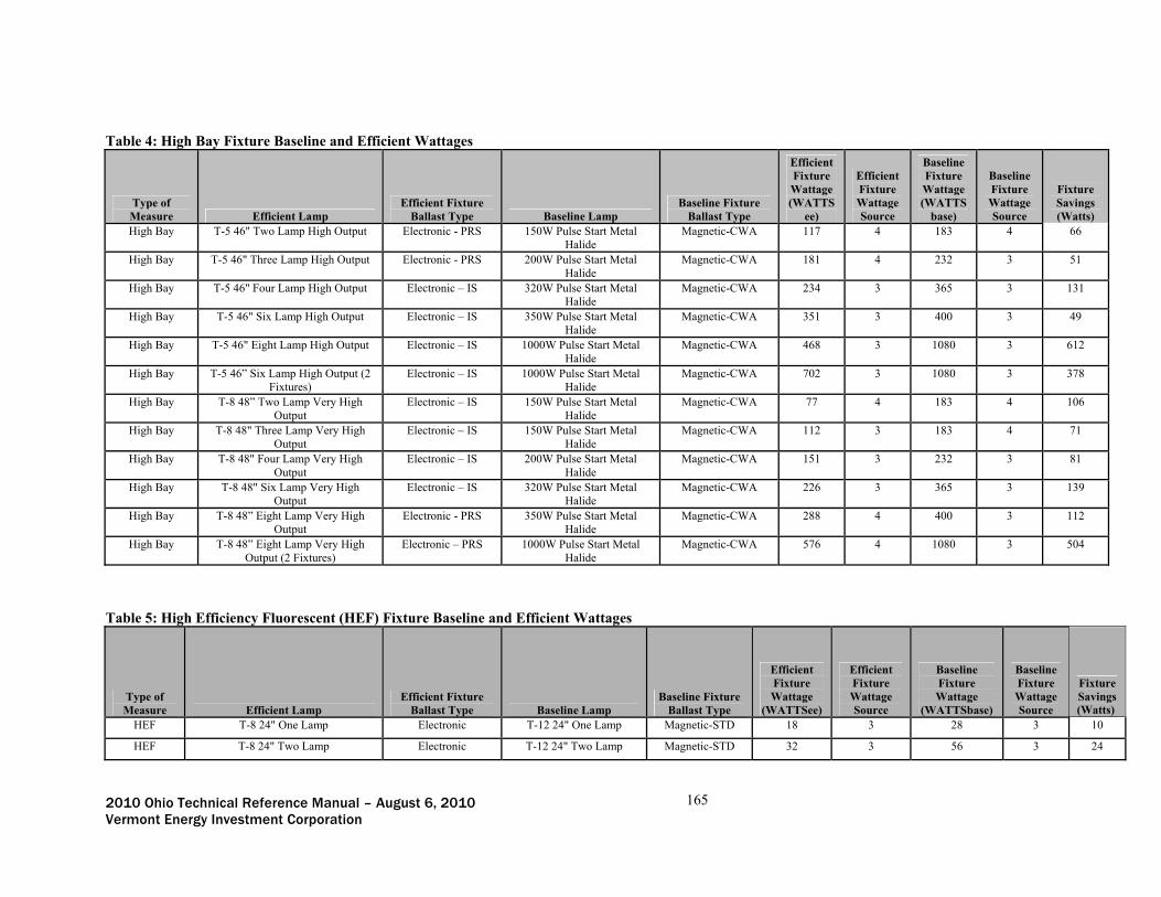
2010 Ohio Technical Reference Manual – August 6, 2010 165 Vermont Energy Investment Corporation
Table 4: High Bay Fixture Baseline and Efficient Wattages
Type of Measure Efficient Lamp
Efficient Fixture Ballast Type Baseline Lamp
Baseline Fixture Ballast Type
Efficient Fixture Wattage (WATTS
ee)
Efficient Fixture Wattage Source
Baseline Fixture Wattage (WATTS
base)
Baseline Fixture Wattage Source
Fixture Savings (Watts)
High Bay T-5 46" Two Lamp High Output Electronic - PRS 150W Pulse Start Metal Halide
Magnetic-CWA 117 4 183 4 66
High Bay T-5 46" Three Lamp High Output Electronic - PRS 200W Pulse Start Metal Halide
Magnetic-CWA 181 4 232 3 51
High Bay T-5 46" Four Lamp High Output Electronic – IS 320W Pulse Start Metal Halide
Magnetic-CWA 234 3 365 3 131
High Bay T-5 46" Six Lamp High Output Electronic – IS 350W Pulse Start Metal Halide
Magnetic-CWA 351 3 400 3 49
High Bay T-5 46" Eight Lamp High Output Electronic – IS 1000W Pulse Start Metal Halide
Magnetic-CWA 468 3 1080 3 612
High Bay T-5 46” Six Lamp High Output (2 Fixtures)
Electronic – IS 1000W Pulse Start Metal Halide
Magnetic-CWA 702 3 1080 3 378
High Bay T-8 48” Two Lamp Very High Output
Electronic – IS 150W Pulse Start Metal Halide
Magnetic-CWA 77 4 183 4 106
High Bay T-8 48" Three Lamp Very High Output
Electronic – IS 150W Pulse Start Metal Halide
Magnetic-CWA 112 3 183 4 71
High Bay T-8 48" Four Lamp Very High Output
Electronic – IS 200W Pulse Start Metal Halide
Magnetic-CWA 151 3 232 3 81
High Bay T-8 48" Six Lamp Very High Output
Electronic – IS 320W Pulse Start Metal Halide
Magnetic-CWA 226 3 365 3 139
High Bay T-8 48” Eight Lamp Very High Output
Electronic - PRS 350W Pulse Start Metal Halide
Magnetic-CWA 288 4 400 3 112
High Bay T-8 48” Eight Lamp Very High Output (2 Fixtures)
Electronic – PRS 1000W Pulse Start Metal Halide
Magnetic-CWA 576 4 1080 3 504
Table 5: High Efficiency Fluorescent (HEF) Fixture Baseline and Efficient Wattages
Type of Measure Efficient Lamp
Efficient Fixture Ballast Type Baseline Lamp
Baseline Fixture Ballast Type
Efficient Fixture Wattage
(WATTSee)
Efficient Fixture Wattage Source
Baseline Fixture Wattage
(WATTSbase)
Baseline Fixture Wattage Source
Fixture Savings (Watts)
HEF T-8 24" One Lamp Electronic T-12 24" One Lamp Magnetic-STD 18 3 28 3 10
HEF T-8 24" Two Lamp Electronic T-12 24" Two Lamp Magnetic-STD 32 3 56 3 24

2010 Ohio Technical Reference Manual – August 6, 2010 166 Vermont Energy Investment Corporation
Type of Measure Efficient Lamp
Efficient Fixture Ballast Type Baseline Lamp
Baseline Fixture Ballast Type
Efficient Fixture Wattage
(WATTSee)
Efficient Fixture Wattage Source
Baseline Fixture Wattage
(WATTSbase)
Baseline Fixture Wattage Source
Fixture Savings (Watts)
HEF T-8 24" Three Lamp Electronic T-12 24" Three Lamp Magnetic-STD 50 3 62 3 12
HEF T-8 24" Four Lamp Electronic T-12 24" Four Lamp Magnetic-STD 65 3 112 3 47
HEF T-8 36" One Lamp Electronic T-12 36" One Lamp Magnetic-STD 25 3 46 3 21
HEF T-8 36" Two Lamp Electronic T-12 36" Two Lamp Magnetic-STD 46 3 81 3 35
HEF T-8 36" Three Lamp Electronic T-12 36" Three Lamp Magnetic-STD 70 3 127 3 57
HEF T-8 36" Four Lamp Electronic T-12 36" Four Lamp Magnetic-STD 88 3 162 3 74
HEF Reduced Wattage T-8 48" One Lamp-28W
Electronic – IS T-8 48" One Lamp Electronic - IS 23.3 2 31 3 7.7
HEF Reduced Wattage T-8 48" Two Lamp-28W
Electronic – IS T-8 48" Two Lamp Electronic - IS 47 2 59 3 12
HEF Reduced Wattage T-8 48" Three Lamp-28W
Electronic – IS T-8 48" Three Lamp Electronic - IS 69.9 2 89 3 19.1
HEF Reduced Wattage T-8 48" Four Lamp-28W
Electronic – IS T-8 48" Four Lamp Electronic - IS 92.6 2 112 3 19.4
HEF Reduced Wattage T-8 48" One Lamp-25W
Electronic – IS T-8 48" One Lamp Electronic - IS 22 2 31 3 9
HEF Reduced Wattage T-8 48" Two Lamp-25W
Electronic – IS T-8 48" Two Lamp Electronic - IS 41 2 59 3 18
HEF Reduced Wattage T-8 48" Three Lamp-25W
Electronic – IS T-8 48" Three Lamp Electronic - IS 61.3 2 89 3 27.7
HEF Reduced Wattage T-8 48" Four Lamp-25W
Electronic – IS T-8 48" Four Lamp Electronic - IS 80.5 2 112 3 31.5
HEF T-8 96" One Lamp Electronic – IS T-12 96" One Lamp-ES Magnetic-STD 58 3 75 3 17
HEF T-8 96" Two Lamp Electronic – IS T-12 96" Two Lamp-ES Magnetic-ES 109 3 123 3 14
HEF T-8 96" Four Lamp Electronic – IS T-12 96" Four Lamp-ES Magnetic-ES 219 3 246 3 27
HEF High Performance T-8 48" One Lamp Electronic T-8 48" One Lamp Electronic - IS 25 6 31 3 6
HEF High Performance T-8 48" Two Lamp Electronic T-8 48" Two Lamp Electronic - IS 48 6 59 3 10
HEF High Performance T-8 48" Three Lamp
Electronic T-8 48" Three Lamp Electronic - IS 73 6 89 3 17
HEF High Performance T-8 48" Four Lamp Electronic T-8 48" Four Lamp Electronic - IS 96 6 112 3 18

2010 Ohio Technical Reference Manual – August 6, 2010 167 Vermont Energy Investment Corporation
Table 6: Metal Halide Track (MHT) Lighting Baseline and Efficient Wattages
Type of Measure Efficient Lamp
Efficient Fixture Ballast
Type Baseline Lamp
Baseline Fixture
Ballast Type
Efficient Fixture Wattage
(WATTSee)
Efficient Fixture Wattage Source
Baseline Fixture Wattage
(WATTSbase)
Baseline Fixture Wattage Source
Fixture Savings (Watts)
MHT Metal Halide 20W Two 50W Halogen
23 1 100 1 77
MHT Metal Halide 39W Two 75W Halogen
43 1 150 1 107
MHT Metal Halide 70W Three 75W Halogen
77 1 225 1 148
Table 7: Ceramic Metal Halide (CMH) Baseline and Efficient Wattages
Type of Measure Efficient Lamp
Efficient Fixture Ballast Type Baseline Lamp
Baseline Fixture Ballast Type
Efficient Fixture Wattage
(WATTSee)
Efficient Fixture Wattage Source
Baseline Fixture Wattage
(WATTSbase)
Baseline Fixture Wattage Source
Fixture Savings (Watts)
CMH Ceramic Metal Halide 20W Two 50W Halogen 26 1 100 1 74
CMH Ceramic Metal Halide 39W Two 75W Halogen 45 1 150 1 105
CMH Ceramic Metal Halide 50W Three 65W Halogen 55 1 195 1 140
CMH Ceramic Metal Halide 70W Three 75W Halogen 79 1 225 1 146
CMH Ceramic Metal Halide 100W Three 90W Halogen 110 1 270 1 160
CMH Ceramic Metal Halide 150W Three 120W Halogen 163 1 360 1 197
Version Date & Revision History Draft: Portfolio # Effective date: Date TRM will become effective End date: Date TRM will cease to be effective (or TBD)

2010 Ohio Technical Reference Manual – August 6, 2010 168 Vermont Energy Investment Corporation
Referenced Documents:
1. Efficiency Vermont Technical Reference User Manual (TRM) Measure Savings Algorithms and Cost Assumptions, February, 19, 2010
2. Kuiken et al, Focus on Energy Evaluation, Business Programs: Deemed Savings Manual V1.0, KEMA, March 22, 2010. 3. 2010 Standard Performance Contract Procedures Manual: Appendix B: 2010 Table of Standard Fixture Wattages. Ver. 1.1, Southern
California Edison. February 25, 2010. Web. Accessed June, 19 2010. <http://www.aesc-inc.com/download/SPC/2010SPCDocs/UnifiedManual/App%20B%20Standard%20Fixture%20Watts.pdf>
4. 2009 EPE Program Downloads. Wattage Table 2009. Web. Accessed September, 26 2009. <http://www.epelectricefficiency.com/downloads.asp?section=ci>.
5. New Jersey Clean Energy Program: Protocols to Measure Resource Savings. December 2007. 6. Thorne and Nadel, Commercial Lighting Retrofits: A Briefing Report for Program Implementers, American Council for an Energy-
Efficient Economy, April 2003.

2010 Ohio Technical Reference Manual – August 6, 2010 169 Vermont Energy Investment Corporation
Lighting Systems (Non-Controls) (Early Replacement, Retrofit) Official Measure Code (Measure Number: X-X-X-X (Program name, End Use) Description This measure relates to the installation of new lighting equipment with efficiency that exceeds that of the existing equipment. This characterization could apply to measures such as compact fluorescent lamps (CFLs) and fixtures, linear fluorescent lamps and fixtures, linear fluorescent fixtures replacing high-intensity discharge (HID) fixtures in high-bay applications, high-intensity discharge (HID) fixtures, and delamping. This measure could relate to the early replacement of an existing unit before the end of its useful life or the retrofit of a unit in an existing facility. Definition of Efficient Equipment In order for this characterization to apply, the efficient equipment must have higher efficiency than the existing equipment. Definition of Baseline Equipment The baseline equipment is the existing equipment before the efficient equipment is installed. Default assumptions of the baseline equipment are presented in the tables below. Deemed Calculation for this Measure
Annual kWh Savings = (WATTSbase – WATTSee) * HOURS * (1 + WHFe) / 1000 Summer Coincident Peak kW Savings = (WATTSbase – WATTSee) * CF * (1 + WHFd) / 1000
Deemed Lifetime of Efficient Equipment The expected measure life is dependent on technology type as below: Measure Type Lifetime Screw-in CFL 3.2 years425 Hardwired CFL 12 years426 High Bay Fluorescent Fixture 15 years426 High Efficiency Linear Fluorescent Fixture 15 years426 Pulse Start Metal Halide 7.5 years427 Metal Halide Track Lighting 15 years428 Ceramic Metal Halide 15 years428 Delamping 10429
425 Kuiken et al, Focus on Energy Evaluation, Business Programs: Deemed Savings Manual V1.0, KEMA, March 22, 2010. Assumes 12,000 hours lamp lifetime with extended burn times per start typical in commercial applications. Assuming 3,730 annual lighting operating hours for the commercial sector from the source document, the lamp lifetime is calculated as: 12,000 / 3,730 = 3.2 years 426 2008 Database for Energy-Efficiency Resources (DEER), Version 2008.2.05, “Effective/Remaining Useful Life Values”, California Public Utilities Commission, December 16, 2008 427 The Energy Independence and Security Act of 2007 requires that as of January 1, 2009, metal halide fixtures designed for use with lamps ≥150 W and ≤500 W must use “probe start” ballasts with ballast efficiency ≥94% or “pulse start” ballasts with ballast efficiency ≥88%. This essentially means that new metal halide fixtures will utilize “pulse start” technology. Assuming that the age of the existing equipment being replaced is half of the total expected lifetime for a metal halide fixture (7.5 years), it is assumed that savings are only achieved for half of the lifetime of the new fixture at which point the customer would have had to replace the inefficient technology with “pulse start” technology negating any savings. 428 Efficiency Vermont Technical Reference User Manual (TRM) Measure Savings Algorithms and Cost Assumptions, February, 19, 2010 429 Based on a review of measure life assumptions in Oregon, California, and Iowa as presented in Measure Life Study, Energy & Resource Solutions, November 17, 2005, delamping lifetime assumptions range from 9 to 16 years. The high end or this range exceeds the assumed fixture lifetime and has been adjusted down to a more conservative 10 years to reflect expected persistence issues.
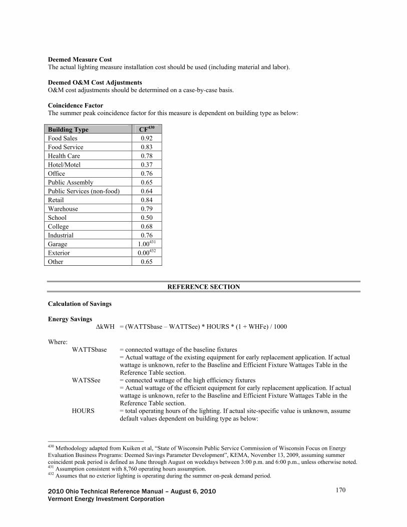
2010 Ohio Technical Reference Manual – August 6, 2010 170 Vermont Energy Investment Corporation
Deemed Measure Cost The actual lighting measure installation cost should be used (including material and labor). Deemed O&M Cost Adjustments O&M cost adjustments should be determined on a case-by-case basis. Coincidence Factor The summer peak coincidence factor for this measure is dependent on building type as below: Building Type CF430 Food Sales 0.92 Food Service 0.83 Health Care 0.78 Hotel/Motel 0.37 Office 0.76 Public Assembly 0.65 Public Services (non-food) 0.64 Retail 0.84 Warehouse 0.79 School 0.50 College 0.68 Industrial 0.76 Garage 1.00431 Exterior 0.00432 Other 0.65
REFERENCE SECTION
Calculation of Savings Energy Savings
ΔkWH = (WATTSbase – WATTSee) * HOURS * (1 + WHFe) / 1000
Where: WATTSbase = connected wattage of the baseline fixtures = Actual wattage of the existing equipment for early replacement application. If actual
wattage is unknown, refer to the Baseline and Efficient Fixture Wattages Table in the Reference Table section.
WATSSee = connected wattage of the high efficiency fixtures = Actual wattage of the efficient equipment for early replacement application. If actual wattage is unknown, refer to the Baseline and Efficient Fixture Wattages Table in the Reference Table section.
HOURS = total operating hours of the lighting. If actual site-specific value is unknown, assume default values dependent on building type as below:
430 Methodology adapted from Kuiken et al, “State of Wisconsin Public Service Commission of Wisconsin Focus on Energy Evaluation Business Programs: Deemed Savings Parameter Development”, KEMA, November 13, 2009, assuming summer coincident peak period is defined as June through August on weekdays between 3:00 p.m. and 6:00 p.m., unless otherwise noted. 431 Assumption consistent with 8,760 operating hours assumption. 432 Assumes that no exterior lighting is operating during the summer on-peak demand period.

2010 Ohio Technical Reference Manual – August 6, 2010 171 Vermont Energy Investment Corporation
Building Type HOURS433 Food Sales 5,544 Food Service 4,482 Health Care 3,677 Hotel/Motel 3,356 Office 3,526 Public Assembly 2,729 Public Services (non-food) 3,425 Retail 4,226 Warehouse 3,464 School 2,302 College 3,900 Industrial – 1 Shift 2,857434 Industrial – 2 Shift 4,730435 Industrial – 3 Shift 6,631436 Exterior 3,833437 Other 3,672
WHFe = lighting-HVAC Interation Factor for energy; this factor represents the reduced electric
space cooling requirements due to the reduction of waste heat rejected by the efficent lighting.
= 0.095 (interior fixtures), 0.000 (exterior fixtures)438 1 / 1000 = conversion factor from watts to kilowatts
Summer Coincident Peak Demand Savings
ΔkW = (WATTSbase – WATTSee) * CF * (1 + WHFd) / 1000
Where: WHFd = lighting-HVAC waste heat factor for demand; this factor represents the reduced electric
space cooling requirements due to the reduction of waste heat rejected by the efficent lighting. = 0.200 (interior fixtures), 0.000 (exterior fixtures)439
433 Kuiken et al, “State of Wisconsin Public Service Commission of Wisconsin Focus on Energy Evaluation Business Programs: Deemed Savings Parameter Development”, KEMA, November 13, 2009, unless otherwise noted. 434 UI and CL&P Program Savings Documentation for 2010 Program Year, United Illuminating Company, September 2009. 435 Ibid. 436 Ibid. 437 Exterior lighting 3,833 hours per year assumes 10.5 hours per day; typical average for photocell control. 438 Interactive factor data based on a series of prototypical small commercial building simulation runs. Values shown are weighted averages across fast food restaurant, full service restaurant, assembly, big box retail, small retail, small office, light industrial and school building models. The prototypes are based on the California DEER study prototypes, modified for local construction practices. Simulations were run using TMY3 weather data for the following Ohio cities: Cincinnati, Cleveland, Columbus and Dayton. Values were weighted based on program participation data for a small commercial program conducted in Indiana for Duke Energy. See An Evaluation of the Indiana Small Commercial and Industrial Incentive Program. Prepared by TecMarket Works for Duke Energy. June 2007. Building prototypes used in the energy modeling are described in Appendix A - Prototypical Building Energy Simulation Model Development. 439 Interactive factor data based on a series of prototypical small commercial building simulation runs. Values shown are weighted averages across fast food restaurant, full service restaurant, assembly, big box retail, small retail, small office, light

2010 Ohio Technical Reference Manual – August 6, 2010 172 Vermont Energy Investment Corporation
CF = Summer Peak Coincidence Factor for measure Dependent on building type as below: Building Type CF440 Food Sales 0.92 Food Service 0.83 Health Care 0.78 Hotel/Motel 0.37 Office 0.76 Public Assembly 0.65 Public Services (non-food) 0.64 Retail 0.84 Warehouse 0.79 School 0.50 College 0.68 Industrial 0.76 Garage 1.00441 Exterior 0.00442 Other 0.65
Fossil Fuel Impact Descriptions and Calculation
ΔMMBtu = ΔkWh * IFMMBtu
Where: IFMMBtu = lighting-HVAC Interation Factor for gas heating impacts; this factor represents the
increased gas space heating requirements due to the reduction of waste heat rejected by the efficent lighting. = -0.0028 (interior fixtures), 0.0000 (exterior fixtures) 443
Water Impact Descriptions and Calculation n/a
industrial and school building models. The prototypes are based on the California DEER study prototypes, modified for local construction practices. Simulations were run using TMY3 weather data for the following Ohio cities: Cincinnati, Cleveland, Columbus and Dayton. Values were weighted based on program participation data for a small commercial program conducted in Indiana for Duke Energy. See An Evaluation of the Indiana Small Commercial and Industrial Incentive Program. Prepared by TecMarket Works for Duke Energy. June 2007. Building prototypes used in the energy modeling are described in Appendix A - Prototypical Building Energy Simulation Model Development. 440 Methodology adapted from Kuiken et al, “State of Wisconsin Public Service Commission of Wisconsin Focus on Energy Evaluation Business Programs: Deemed Savings Parameter Development”, KEMA, November 13, 2009, assuming summer coincident peak period is defined as June through August on weekdays between 3:00 p.m. and 6:00 p.m., unless otherwise noted. 441 Assumption consistent with 8,760 operating hours assumption. 442 Assumes that no exterior lighting is operating during the summer on-peak demand period. 443 Interactive factor data based on a series of prototypical small commercial building simulation runs. Values shown are weighted averages across fast food restaurant, full service restaurant, assembly, big box retail, small retail, small office, light industrial and school building models. The prototypes are based on the California DEER study prototypes, modified for local construction practices. Simulations were run using TMY3 weather data for the following Ohio cities: Cincinnati, Cleveland, Columbus and Dayton. Values were weighted based on program participation data for a small commercial program conducted in Indiana for Duke Energy. See An Evaluation of the Indiana Small Commercial and Industrial Incentive Program. Prepared by TecMarket Works for Duke Energy. June 2007. Building prototypes used in the energy modeling are described in Appendix A - Prototypical Building Energy Simulation Model Development.
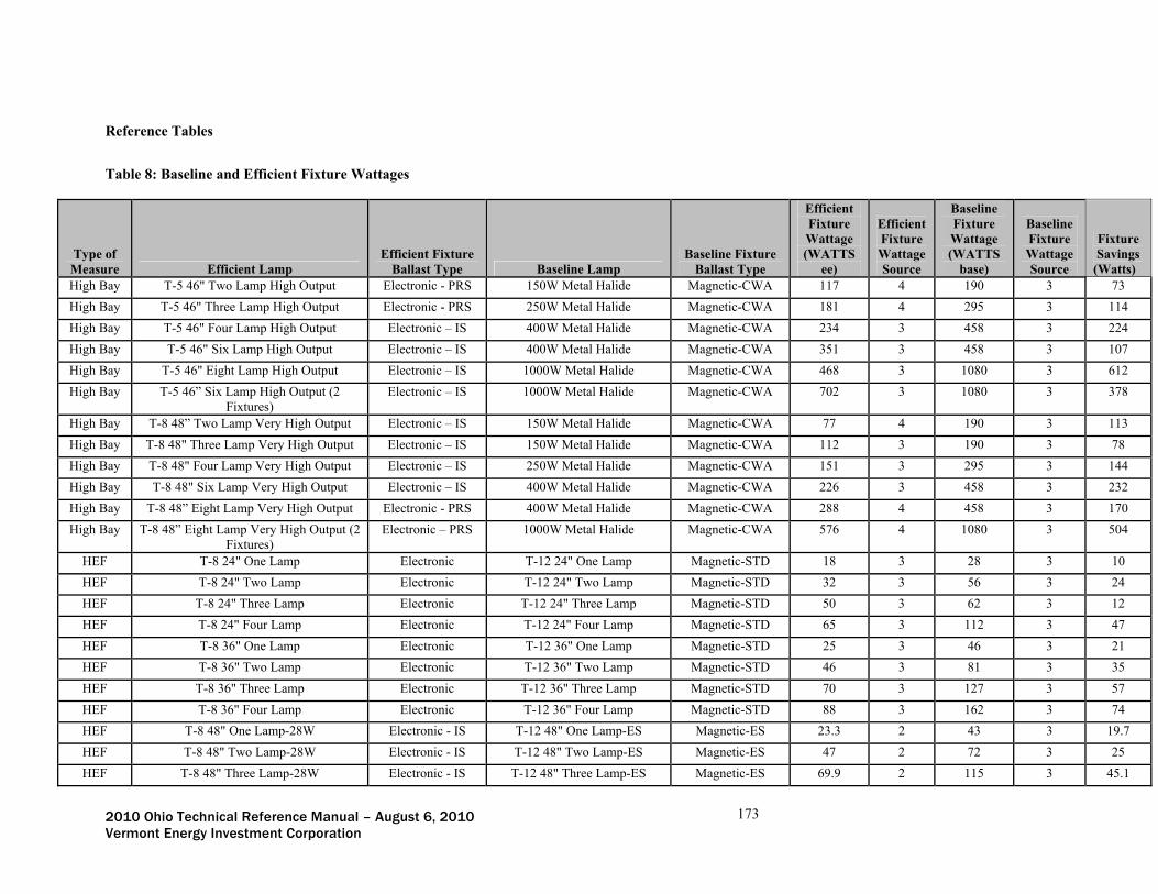
2010 Ohio Technical Reference Manual – August 6, 2010 173 Vermont Energy Investment Corporation
Reference Tables
Table 8: Baseline and Efficient Fixture Wattages
Type of Measure Efficient Lamp
Efficient Fixture Ballast Type Baseline Lamp
Baseline Fixture Ballast Type
Efficient Fixture Wattage (WATTS
ee)
Efficient Fixture Wattage Source
Baseline Fixture Wattage (WATTS
base)
Baseline Fixture Wattage Source
Fixture Savings
(Watts) High Bay T-5 46" Two Lamp High Output Electronic - PRS 150W Metal Halide Magnetic-CWA 117 4 190 3 73
High Bay T-5 46" Three Lamp High Output Electronic - PRS 250W Metal Halide Magnetic-CWA 181 4 295 3 114
High Bay T-5 46" Four Lamp High Output Electronic – IS 400W Metal Halide Magnetic-CWA 234 3 458 3 224
High Bay T-5 46" Six Lamp High Output Electronic – IS 400W Metal Halide Magnetic-CWA 351 3 458 3 107
High Bay T-5 46" Eight Lamp High Output Electronic – IS 1000W Metal Halide Magnetic-CWA 468 3 1080 3 612
High Bay T-5 46” Six Lamp High Output (2 Fixtures)
Electronic – IS 1000W Metal Halide Magnetic-CWA 702 3 1080 3 378
High Bay T-8 48” Two Lamp Very High Output Electronic – IS 150W Metal Halide Magnetic-CWA 77 4 190 3 113
High Bay T-8 48" Three Lamp Very High Output Electronic – IS 150W Metal Halide Magnetic-CWA 112 3 190 3 78
High Bay T-8 48" Four Lamp Very High Output Electronic – IS 250W Metal Halide Magnetic-CWA 151 3 295 3 144
High Bay T-8 48" Six Lamp Very High Output Electronic – IS 400W Metal Halide Magnetic-CWA 226 3 458 3 232
High Bay T-8 48” Eight Lamp Very High Output Electronic - PRS 400W Metal Halide Magnetic-CWA 288 4 458 3 170
High Bay T-8 48” Eight Lamp Very High Output (2 Fixtures)
Electronic – PRS 1000W Metal Halide Magnetic-CWA 576 4 1080 3 504
HEF T-8 24" One Lamp Electronic T-12 24" One Lamp Magnetic-STD 18 3 28 3 10
HEF T-8 24" Two Lamp Electronic T-12 24" Two Lamp Magnetic-STD 32 3 56 3 24
HEF T-8 24" Three Lamp Electronic T-12 24" Three Lamp Magnetic-STD 50 3 62 3 12
HEF T-8 24" Four Lamp Electronic T-12 24" Four Lamp Magnetic-STD 65 3 112 3 47
HEF T-8 36" One Lamp Electronic T-12 36" One Lamp Magnetic-STD 25 3 46 3 21
HEF T-8 36" Two Lamp Electronic T-12 36" Two Lamp Magnetic-STD 46 3 81 3 35
HEF T-8 36" Three Lamp Electronic T-12 36" Three Lamp Magnetic-STD 70 3 127 3 57
HEF T-8 36" Four Lamp Electronic T-12 36" Four Lamp Magnetic-STD 88 3 162 3 74
HEF T-8 48" One Lamp-28W Electronic - IS T-12 48" One Lamp-ES Magnetic-ES 23.3 2 43 3 19.7
HEF T-8 48" Two Lamp-28W Electronic - IS T-12 48" Two Lamp-ES Magnetic-ES 47 2 72 3 25
HEF T-8 48" Three Lamp-28W Electronic - IS T-12 48" Three Lamp-ES Magnetic-ES 69.9 2 115 3 45.1

2010 Ohio Technical Reference Manual – August 6, 2010 174 Vermont Energy Investment Corporation
Type of Measure Efficient Lamp
Efficient Fixture Ballast Type Baseline Lamp
Baseline Fixture Ballast Type
Efficient Fixture Wattage (WATTS
ee)
Efficient Fixture Wattage Source
Baseline Fixture Wattage (WATTS
base)
Baseline Fixture Wattage Source
Fixture Savings
(Watts) HEF T-8 48" Four Lamp-28W Electronic - IS T-12 48" Four Lamp-ES Magnetic-ES 92.6 2 144 3 51.4
HEF T-8 48" One Lamp-25W Electronic - IS T-12 48" One Lamp-ES Magnetic-ES 22 2 43 3 21
HEF T-8 48" Two Lamp-25W Electronic - IS T-12 48" Two Lamp-ES Magnetic-ES 41 2 72 3 31
HEF T-8 48" Three Lamp-25W Electronic - IS T-12 48" Three Lamp-ES Magnetic-ES 61.3 2 115 3 53.7
HEF T-8 48" Four Lamp-25W Electronic - IS T-12 48" Four Lamp-ES Magnetic-ES 80.5 2 144 3 63.5
HEF T-8 96" One Lamp Electronic - IS T-12 96" One Lamp-ES Magnetic-STD 58 3 75 3 17
HEF T-8 96" Two Lamp Electronic - IS T-12 96" Two Lamp-ES Magnetic-ES 109 3 123 3 14
HEF T-8 96" Four Lamp Electronic - IS T-12 96" Four Lamp-ES Magnetic-ES 219 3 246 3 27
HEF High Performance T-8 48" One Lamp Electronic T-12 48" One Lamp-ES Magnetic-ES 25 6 43 3 18
HEF High Performance T-8 48" Two Lamp Electronic T-12 48" Two Lamp-ES Magnetic-ES 48 6 72 3 23
HEF High Performance T-8 48" Three Lamp Electronic T-12 48" Three Lamp-ES Magnetic-ES 73 6 115 3 43
HEF High Performance T-8 48" Four Lamp Electronic T-12 48" Four Lamp-ES Magnetic-ES 96 6 144 3 50
MHT Metal Halide 20W Two 50W Halogen 23 1 100 1 77
MHT Metal Halide 39W Two 75W Halogen 43 1 150 1 107
MHT Metal Halide 70W Three 75W Halogen 77 1 225 1 148
CMH Ceramic Metal Halide 20W Two 50W Halogen 26 1 100 1 74
CMH Ceramic Metal Halide 39W Two 75W Halogen 45 1 150 1 105
CMH Ceramic Metal Halide 50W Three 65W Halogen 55 1 195 1 140
CMH Ceramic Metal Halide 70W Three 75W Halogen 79 1 225 1 146
CMH Ceramic Metal Halide 100W Three 90W Halogen 110 1 270 1 160
CMH Ceramic Metal Halide 150W Three 120W Halogen 163 1 360 1 197
Delamp No Lamp Magnetic-STD T-12 18” One Lamp Magnetic-STD 4 TBD 19 3 15
Delamp No Lamp No Ballast T-12 18” One Lamp Magnetic-STD 0 TBD 19 3 19
Delamp No Lamp Magnetic-STD T-12 24” One Lamp Magnetic-STD 8 TBD 28 3 20
Delamp No Lamp No Ballast T-12 24” One Lamp Magnetic-STD 0 TBD 28 3 28
Delamp No Lamp Magnetic-STD T-12 36” One Lamp Magnetic-STD 16 TBD 46 3 30
Delamp No Lamp No Ballast T-12 36” One Lamp Magnetic-STD 0 TBD 46 3 46
Delamp No Lamp Magnetic-STD T-12 48” One Lamp Magnetic-STD 21 TBD 60 3 39
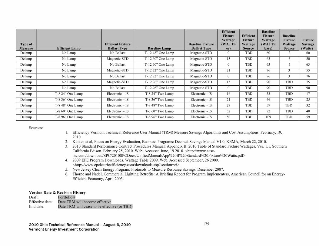
2010 Ohio Technical Reference Manual – August 6, 2010 175 Vermont Energy Investment Corporation
Type of Measure Efficient Lamp
Efficient Fixture Ballast Type Baseline Lamp
Baseline Fixture Ballast Type
Efficient Fixture Wattage (WATTS
ee)
Efficient Fixture Wattage Source
Baseline Fixture Wattage (WATTS
base)
Baseline Fixture Wattage Source
Fixture Savings
(Watts) Delamp No Lamp No Ballast T-12 48” One Lamp Magnetic-STD 0 TBD 60 3 60
Delamp No Lamp Magnetic-STD T-12 60” One Lamp Magnetic-STD 13 TBD 63 3 50
Delamp No Lamp No Ballast T-12 60” One Lamp Magnetic-STD 0 TBD 63 3 63
Delamp No Lamp Magnetic-STD T-12 72” One Lamp Magnetic-STD 21 TBD 76 3 55
Delamp No Lamp No Ballast T-12 72” One Lamp Magnetic-STD 0 TBD 76 3 76
Delamp No Lamp Magnetic-STD T-12 96” One Lamp Magnetic-STD 15 TBD 90 TBD 75
Delamp No Lamp No Ballast T-12 96” One Lamp Magnetic-STD 0 TBD 90 TBD 90
Delamp T-8 24” One Lamp Electronic – IS T-8 24” Two Lamp Electronic - IS 16 TBD 33 TBD 17
Delamp T-8 36” One Lamp Electronic – IS T-8 36” Two Lamp Electronic - IS 21 TBD 46 TBD 25
Delamp T-8 48” One Lamp Electronic – IS T-8 48” Two Lamp Electronic - IS 27 TBD 59 TBD 32
Delamp T-8 60” One Lamp Electronic – IS T-8 60” Two Lamp Electronic - IS 32 TBD 72 TBD 40
Delamp T-8 96” One Lamp Electronic – IS T-8 96” Two Lamp Electronic - IS 50 TBD 109 TBD 59
Sources:
1. Efficiency Vermont Technical Reference User Manual (TRM) Measure Savings Algorithms and Cost Assumptions, February, 19, 2010
2. Kuiken et al, Focus on Energy Evaluation, Business Programs: Deemed Savings Manual V1.0, KEMA, March 22, 2010. 3. 2010 Standard Performance Contract Procedures Manual: Appendix B: 2010 Table of Standard Fixture Wattages. Ver. 1.1, Southern
California Edison. February 25, 2010. Web. Accessed June, 19 2010. <http://www.aesc-inc.com/download/SPC/2010SPCDocs/UnifiedManual/App%20B%20Standard%20Fixture%20Watts.pdf>
4. 2009 EPE Program Downloads. Wattage Table 2009. Web. Accessed September, 26 2009. <http://www.epelectricefficiency.com/downloads.asp?section=ci>.
5. New Jersey Clean Energy Program: Protocols to Measure Resource Savings. December 2007. 6. Thorne and Nadel, Commercial Lighting Retrofits: A Briefing Report for Program Implementers, American Council for an Energy-
Efficient Economy, April 2003.
Version Date & Revision History Draft: Portfolio # Effective date: Date TRM will become effective End date: Date TRM will cease to be effective (or TBD)

2010 Ohio Technical Reference Manual – August 6, 2010 176 Vermont Energy Investment Corporation
Lighting Power Density Reduction (New Construction) Official Measure Code (Measure Number: X-X-X-X (Program name, End Use) Description This measure relates to the implementation of various lighting design principles aimed at creating a quality and appropriate lighting experience while reducing unnecessary light usage. This is often done by a professional in a new construction situation. Techniques like maximizing daylighting, task lighting, lighting controls, and efficient fixtures are used to create a system of optimal functionality while reducing total lighting power density. Definition of Efficient Equipment In order for this characterization to apply, this measure assumes the high efficiency equipment consists of a lighting system that exceeds the lighting power density requirements as mandated by the International Energy Conservation Code (IECC) 2006, Table 505.5.2. Definition of Baseline Equipment The baseline efficiency assumes compliance with lighting power density requirements as mandated by the International Energy Conservation Code (IECC) 2006, Table 505.5.2.
Deemed Calculation for this Measure
Annual kWh Savings = (WATTSbase – WATTSee) / 1000 * AREA * HOURS * (1 +WHFe)
Summer Coincident Peak kW Savings = (WATTSbase – WATTSee) / 1000 * AREA * (1 + WHFd) * CF Deemed Lifetime of Efficient Equipment The expected measure life is measure is 15 years444. Deemed Measure Cost The incremental capital costs for this measure vary by the assumed baseline and efficient equipment scenarios. Incremental costs by measure type are presented below: Coincidence Factor The summer peak coincidence factor for this measure is dependent on building type as below:
Building Type CF445 Food Sales 0.92 Food Service 0.83 Health Care 0.78 Hotel/Motel 0.37 Office 0.76 Public Assembly 0.65 Public Services (non-food) 0.64 Retail 0.84 Warehouse 0.79 School 0.50
444 Measure Life Report, Residential and Commercial/Industrial Lighting and HVAC Measures, GDS Associates, June 2007. http://www.ctsavesenergy.org/files/Measure%20Life%20Report%202007.pdf 445 Methodology adapted from Kuiken et al, “State of Wisconsin Public Service Commission of Wisconsin Focus on Energy Evaluation Business Programs: Deemed Savings Parameter Development”, KEMA, November 13, 2009, assuming summer coincident peak period is defined as June through August on weekdays between 3:00 p.m. and 6:00 p.m., unless otherwise noted.

2010 Ohio Technical Reference Manual – August 6, 2010 177 Vermont Energy Investment Corporation
Building Type CF445 College 0.68 Industrial 0.76 Garage 1.00446 Other 0.65
REFERENCE SECTION
Calculation of Savings Energy Savings
ΔkWh = ((WATTSbase – WATTSee) / 1000 * AREA * HOURS * (1 +WHFe)
Where: WATTSbase447 = allowed lighting wattage per square foot based on energy code requirements for
building type; see table below for values:
Building Area Type Lighting Power Density (W/ft2) Automotive Facility 0.9 Convention Center 1.2 Court House 1.2 Dining: Bar Lounge/Leisure 1.3 Dining: Cafeteria/Fast Food 1.4 Dining: Family 1.6 Dormitory 1.0 Exercise Center 1.0 Gymnasium 1.1 Healthcare-Clinic 1.0 Hospital/Healthcare 1.2 Hotel 1.0 Library 1.3 Manufacturing Facility 1.3 Motel 1.0 Motion Picture Theatre 1.2 Multi-Family 0.7 Museum 1.1 Office 1.0 Parking Garage 0.3 Penitentiary 1.0 Performing Arts Theatre 1.6 Police/Fire Station 1.0 Post Office 1.1 Religious Building 1.3 Retail 1.5 School/University 1.2
446 Assumption consistent with 8,760 operating hours assumption. 447 International Energy Conservation Code (IECC 2006) 2006, Table 505.5.2, Interior Lighting Power Allowances

2010 Ohio Technical Reference Manual – August 6, 2010 178 Vermont Energy Investment Corporation
Building Area Type Lighting Power Density (W/ft2) Sports Arena 1.1 Town Hall 1.1 Transportation 1.0 Warehouse 0.8 Workshop 1.4
WATSSee = actual installed lighting wattage per square foot of the efficient lighting system for
building type as determined by site-surveys or design diagrams. 1000 = conversion factor (W / kW) AREA = area of the building in square feet; determined from site-specific information HOURS = annual site-specific hours of operation of the lighting equipment; dependent on building
type as below: Building Type HOURS448 Food Sales 5,544 Food Service 4,482 Health Care 3,677 Hotel/Motel 3,356 Office 3,526 Public Assembly 2,729 Public Services (non-food) 3,425 Retail 4,226 Warehouse 3,464 School 2,302 College 3,900 Industrial 4,745 Garage 8,760449 Other 3,672
WHFe = lighting-HVAC Interation Factor for energy; this factor represents the reduced electric
space cooling requirements due to the reduction of waste heat rejected by the efficent lighting.
= 0.095 (interior fixtures), 0.000 (exterior fixtures)450 Summer Coincident Peak Demand Savings
ΔkW = (WATTSbase – WATTSee) * CF * (1 + WHFd) / 1000
Where:
448 Kuiken et al, “State of Wisconsin Public Service Commission of Wisconsin Focus on Energy Evaluation Business Programs: Deemed Savings Parameter Development”, KEMA, November 13, 2009 449 Assumes operation 24 hours per day, 365 days per year. 450 Interactive factor data based on a series of prototypical small commercial building simulation runs. Values shown are weighted averages across fast food restaurant, full service restaurant, assembly, big box retail, small retail, small office, light industrial and school building models. The prototypes are based on the California DEER study prototypes, modified for local construction practices. Simulations were run using TMY3 weather data for the following Ohio cities: Cincinnati, Cleveland, Columbus and Dayton. Values were weighted based on program participation data for a small commercial program conducted in Indiana for Duke Energy. See An Evaluation of the Indiana Small Commercial and Industrial Incentive Program. Prepared by TecMarket Works for Duke Energy. June 2007. Building prototypes used in the energy modeling are described in Appendix A - Prototypical Building Energy Simulation Model Development.

2010 Ohio Technical Reference Manual – August 6, 2010 179 Vermont Energy Investment Corporation
WHFd = lighting-HVAC waste heat factor for demand; this factor represents the reduced electric space cooling requirements due to the reduction of waste heat rejected by the efficent lighting. = 0.200 (interior fixtures), 0.000 (exterior fixtures)419
CF = Summer Peak Coincidence Factor for measure Dependent on building type as below: Building Type CF451 Food Sales 0.92 Food Service 0.83 Health Care 0.78 Hotel/Motel 0.37 Office 0.76 Public Assembly 0.65 Public Services (non-food) 0.64 Retail 0.84 Warehouse 0.79 School 0.50 College 0.68 Industrial 0.76 Garage 1.00452 Other 0.65
Fossil Fuel Impact Descriptions and Calculation TBD453 Water Impact Descriptions and Calculation n/a Deemed O&M Cost Adjustment Calculation n/a Referenced Documents: “Draft TRM - C&I Buildings Model Development.doc”
451 Methodology adapted from Kuiken et al, “State of Wisconsin Public Service Commission of Wisconsin Focus on Energy Evaluation Business Programs: Deemed Savings Parameter Development”, KEMA, November 13, 2009, assuming summer coincident peak period is defined as June through August on weekdays between 3:00 p.m. and 6:00 p.m., unless otherwise noted. 452 Assumption consistent with 8,760 operating hours assumption. 453 This section pending further information from utilities regarding the energy simulation models used to derive the lighting-HVAC interaction factors.

2010 Ohio Technical Reference Manual – August 6, 2010 180 Vermont Energy Investment Corporation
LED Case Lighting with/without Motion Sensors (New Construction; Retrofit – Early Replacement Official Measure Code (Measure Number: X-X-X-X (Program name, End Use) Description This measure relates to the installation of LED lamps with and without motion sensors in vertical display refrigerators, coolers, and freezers replacing T8 or T12 linear fluorescent lamp technology. LED lamps should be systems intended for this application. LED lamps not only provide the same light output with lower connected wattages, but also produce less waste heat which decreases the cooling load on the refrigeration system and energy needed by the refrigerator compressor. Additional savings can be achieved from the installation of a motion sensor which automatically dims the lighting system when the space is unoccupied. Retrofit projects must completely remove the existing fluorescent fixture end connectors and ballasts to qualify, though wiring may be reused. Eligible fixtures include new, replacement, and retrofit. Savings and assumptions are based on a per door basis. Definition of Efficient Equipment In order for this characterization to apply, the efficient equipment is assumed to be LED case lighting with or without motion sensors on refrigerators, coolers, and freezers - specifically on vertical displays. Definition of Baseline Equipment In order for this characterization to apply, the baseline equipment is assumed to be T8 or T12 linear fluorescent lamps. Deemed Calculation for this Measure
Annual kWh Savings = (WATTSbase – WATTSee) / 1000 * Ndoors * HOURS * (1 + WHFe) *
ESFMC Summer Coincident Peak kW Savings = (WATTSbase – WATTSee) / 1000 * Ndoors * (1 + WHFd) * CF
Deemed Lifetime of Efficient Equipment The expected measure life is assumed to be 8.1 years454. Deemed Measure Cost The incremental capital cost for this measure is $250 per door (retrofit), and $150 (time of sale, new construction)455. If a motion sensor is installed, add an additional cost of $130 per 25ft of case456. Deemed O&M Cost Adjustments The stream of baseline lamp replacement costs over the lifetime of the measure results in a Net Present Value457 of $22.96. This computes to a levelized annual baseline replacement cost assumption of $4.07. Coincidence Factor The summer peak coincidence factor for this measure is assumed to be 92%458. 454 Theobald, M. A., Emerging Technologies Program: Application Assessment Report #0608, LED Supermarket Case Lighting Grocery Store, Northern California, Pacific Gas and Electric Company, January 2006. Assumes annual operating hours of 6,205. <http://www.etcc-ca.com/images/stories/pdf/ETCC_Report_204.pdf>. The lifetime of the motion sensors is assumed to be equal to the lifetime of the LED lighting. 455 Based on a review of TRM incremental cost assumptions from Oregon and Vermont, supplemented with completed project information from New York. 456 “LED Case Lighting With and Without Motion Sensors” presentation, Michele Friedrich, PECI, January 2010. 457 Using a discount rate of 5.7% (as is used for Efficiency Vermont). Assumes baseline ballast life exceeds the life of the LED assembly.

2010 Ohio Technical Reference Manual – August 6, 2010 181 Vermont Energy Investment Corporation
REFERENCE SECTION
Calculation of Savings Energy Savings
ΔkWh = (WATTSbase – WATTSee) / 1000 * Ndoors * HOURS * (1 + WHFe) * ESFMC
Where:
WATTSbase = connected wattage per door of the baseline fixtures; see table below for default values. WATTSee = connected wattage per door of the high efficiency fixtures = Actual installed. If actual installed wattage is unknown, see table below for default
values.
LED Refrigerated Case Lighting System Baseline and Efficient Wattages459
1000 = conversion factor from watts to kilowatts Ndoors = number of doors = Actual installed HOURS = annual operating hours; assume 6,205 operating hours per year460 if actual operating
hours are unknown ESFMC = Energy Savings Factor; additional savings percentage achieved with a motion sensor.
Assume a value of 1.0 if no motion sensor is installed, or 1.43 if motion sensor is installed.461
WHFe = waste heat factor for energy to account for cooling savings from efficient lighting. For prescriptive refrigerated lighting measures, the default value is 0.41 for refrigerated space and 0.52 for freezer space462.
Summer Coincident Peak Demand Savings
458 Methodology adapted from Kuiken et al, “State of Wisconsin Public Service Commission of Wisconsin Focus on Energy Evaluation Business Programs: Deemed Savings Parameter Development”, KEMA, November 13, 2009, assuming summer coincident peak period is defined as June through August on weekdays between 3:00 p.m. and 6:00 p.m., unless otherwise noted. 459 From Pacific Gas & Electric ‘LED Refrig Lighting ERCO_Talking_Points_v3.pdf.’ The efficient wattage, 38 and 46 watts, are the maximum allowed watts for a 5-foot and 6-foot LED refrigerated case lighting system that meets the efficiency specifications of the Designlights Consortium. 460 Theobald, M. A., Emerging Technologies Program: Application Assessment Report #0608, LED Supermarket Case Lighting Grocery Store, Northern California, Pacific Gas and Electric Company, January 2006. Assumes refrigerated case lighting typically operates 17 hours per day, 365 days per year. <http://www.etcc-ca.com/images/stories/pdf/ETCC_Report_204.pdf> 461 D. Bisbee, Sacramento Municipal Utility District, “Customer Advanced Technologies Program Technology Evaluation Report: LED Freezer Case Lighting Systems”, July 2008. 462 Values adopted from Hall, N. et al, New York Standard Approach for Estimating Energy Savings from Energy Efficiency Measures in Commercial and Industrial Programs, TecMarket Works, September 1, 2009. This factor is a candidate from future adjustment due to climatic differences between Ohio and New York.
Fixture Savings Type of
Measure Efficient Lamp Baseline Lamp
Efficient Fixture Wattage (WATTS
ee)
Baseline Fixture Wattage (WATTS
base) (Watts) Refrigerated
Case Lighting per door
5’ LED Case Lighting System 5’ T8 Case Lighting System 38 76 38
Refrigerated Case Lighting
per door 6’ LED Case Lighting System
6’ T12HO Case Lighting System
46 112 66

2010 Ohio Technical Reference Manual – August 6, 2010 182 Vermont Energy Investment Corporation
ΔkW = (WATTSbase – WATTSee) / 1000 * Ndoors * (1 + WHFd) * CF
Where: WHFd = waste heat factor for energy to account for cooling savings from efficient lighting. For
prescriptive refrigerated lighting measures, the default value is 0.41 for refrigerated space and 0.52 for freezer space463.
CF = Summer Peak Coincidence Factor for measure = 0.92464 (lighting in food sales)
Fossil Fuel Impact Descriptions and Calculation n/a Water Impact Descriptions and Calculation n/a Deemed O&M Cost Adjustment Calculation The stream of baseline lamp replacement costs over the lifetime of the measure results in a Net Present Value465 of $22.96. This computes to a levelized annual baseline replacement cost assumption of $4.07. Baseline Lamp Cost: $4 Baseline Lamp Life: 12,000 Baseline Lamp Labor Cost: $5.00 (15 min @ $20 per hour labor) Version Date & Revision History Draft: Portfolio # Effective date: Date TRM will become effective End date: Date TRM will cease to be effective (or TBD)
463 Values adopted from Hall, N. et al, New York Standard Approach for Estimating Energy Savings from Energy Efficiency Measures in Commercial and Industrial Programs, TecMarket Works, September 1, 2009. This factor is a candidate from future adjustment due to climatic differences between Ohio and New York. 464 Methodology adapted from Kuiken et al, “State of Wisconsin Public Service Commission of Wisconsin Focus on Energy Evaluation Business Programs: Deemed Savings Parameter Development”, KEMA, November 13, 2009, assuming summer coincident peak period is defined as June through August on weekdays between 3:00 p.m. and 6:00 p.m., unless otherwise noted. 465 Using a discount rate of 5.7% (as is used for Efficiency Vermont). Assumes baseline ballast life exceeds the life of the LED assembly.

2010 Ohio Technical Reference Manual – August 6, 2010 183 Vermont Energy Investment Corporation
LED Exit Signs (Retrofit) Official Measure Code (Measure Number: X-X-X-X (Program name, End Use) Description These exit signs have a string of very small, typically red or green, glowing LEDs arranged in a circle or oval. The LEDs may also be arranged in a line on the side, top or bottom of the exit sign. LED exit signs provide the best balance of safety, low maintenance, and very low energy usage compared to other exit sign technologies. Definition of Efficient Equipment The efficient equipment is assumed to be an exit sign illuminated by light emitting diodes. Definition of Baseline Equipment The baseline equipment is assumed to be a fluorescent model. Deemed Savings for this Measure
Annual kWh Savings = 83 kWh
Summer Coincident Peak kW Savings = 0.010 kW
Deemed Lifetime of Efficient Equipment 16 years466 Deemed Measure Cost $30467 Deemed O&M Cost Adjustments The stream of replacement costs over the lifetime of the measure results in a Net Present Value of $59. This computes to a levelized annual baseline replacement cost assumption of $6.04.468 Coincidence Factor The summer peak coincidence factor for this measure is assumed to be 100%469.
REFERENCE SECTION
Calculation of Savings Energy Savings
ΔkWH = kWSave x HOURS x ISR x WHFe
Where: kWSave = The difference in connected load between baseline equipment and efficient equipment = 0.009470 HOURS = Annual operating hours
466 2008 Database for Energy-Efficiency Resources (DEER), Version 2008.2.05, “Effective/Remaining Useful Life Values”, California Public Utilities Commission, December 16, 2008. 467 NYSERDA Deemed Savings Database, Labor cost assumes 25 minutes @ $18/hr. 468 This calculation assumes a replacement baseline CFL costs $4 with an estimated labor cost of $5 (assuming 20$/hour and a task time of 15 minutes). Lamp life is approximated as 2 years, assuming a 16,000 hour lamp life operating 8,760 hours per year. 469 Assuming continuous operation of an LED exit sign, the Summer Peak Coincidence Factor is assumed to equal 1.0. 470 Efficiency Vermont Technical Reference User Manual (TRM) Measure Savings Algorithms and Cost Assumptions, February, 19, 2010
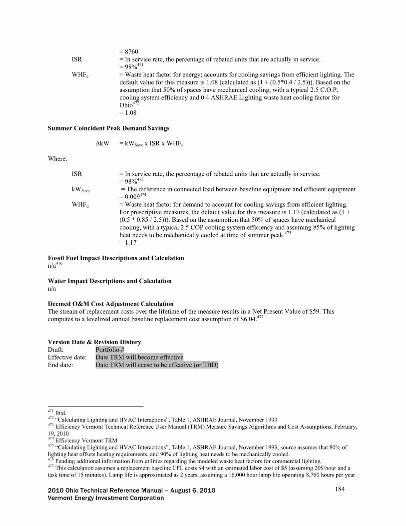
2010 Ohio Technical Reference Manual – August 6, 2010 184 Vermont Energy Investment Corporation
= 8760 ISR = In service rate, the percentage of rebated units that are actually in service.
= 98%471 WHFe = Waste heat factor for energy; accounts for cooling savings from efficient lighting. The
default value for this measure is 1.08 (calculated as (1 + (0.5*0.4 / 2.5))). Based on the assumption that 50% of spaces have mechanical cooling, with a typical 2.5 C.O.P. cooling system efficiency and 0.4 ASHRAE Lighting waste heat cooling factor for Ohio472
= 1.08 Summer Coincident Peak Demand Savings
ΔkW = kWSave x ISR x WHFd
Where:
ISR = In service rate, the percentage of rebated units that are actually in service.
= 98%473 kWSave = The difference in connected load between baseline equipment and efficient equipment = 0.009474 WHFd = Waste heat factor for demand to account for cooling savings from efficient lighting.
For prescriptive measures, the default value for this measure is 1.17 (calculated as (1 + (0.5 * 0.85 / 2.5))). Based on the assumption that 50% of spaces have mechanical cooling, with a typical 2.5 COP cooling system efficiency and assuming 85% of lighting heat needs to be mechanically cooled at time of summer peak.475
= 1.17
Fossil Fuel Impact Descriptions and Calculation n/a476 Water Impact Descriptions and Calculation n/a Deemed O&M Cost Adjustment Calculation The stream of replacement costs over the lifetime of the measure results in a Net Present Value of $59. This computes to a levelized annual baseline replacement cost assumption of $6.04.477 Version Date & Revision History Draft: Portfolio # Effective date: Date TRM will become effective End date: Date TRM will cease to be effective (or TBD)
471 Ibid. 472 “Calculating Lighting and HVAC Interactions”, Table 1, ASHRAE Journal, November 1993 473 Efficiency Vermont Technical Reference User Manual (TRM) Measure Savings Algorithms and Cost Assumptions, February, 19, 2010 474 Efficiency Vermont TRM 475 “Calculating Lighting and HVAC Interactions”, Table 1, ASHRAE Journal, November 1993; source assumes that 80% of lighting heat offsets heating requirements, and 90% of lighting heat needs to be mechanically cooled. 476 Pending additional information from utilities regarding the modeled waste heat factors for commercial lighting. 477 This calculation assumes a replacement baseline CFL costs $4 with an estimated labor cost of $5 (assuming 20$/hour and a task time of 15 minutes). Lamp life is approximated as 2 years, assuming a 16,000 hour lamp life operating 8,760 hours per year.

2010 Ohio Technical Reference Manual – August 6, 2010 185 Vermont Energy Investment Corporation
Traffic Signals (Retrofit) Official Measure Code (Measure Number: X-X-X-X (Program name, End Use) Description Traffic and pedestrian signals are illuminated with light emitting diodes (LED) instead of incandescent lamps. Definition of Efficient Equipment Refer to the Table titled ‘Traffic Signals Technology Equivalencies’ for efficient technology wattage and savings assumptions. Definition of Baseline Equipment Refer to the Table titled ‘Traffic Signals Technology Equivalencies’ for baseline efficiencies and savings assumptions. Deemed Savings for this Measure
Annual kWh Savings = (Wbase – Weff) x HOURS / 1000
Summer Coincident Peak kW Savings = (Wbase– Weff) x CF / 1000
Deemed Lifetime of Efficient Equipment The assumed lifetime of an LED traffic signal is 100,000 hours (manufacturer’s estimate), capped at 10 years.478 The life in years is calculated by dividing 100,000 hrs by the annual operating hours for the particular signal type. Deemed Measure Cost The actual measure installation cost should be used (including material and labor). Deemed O&M Cost Adjustments479 Because LEDs last much longer than incandescent bulbs, LEDs offer operation and maintenance (O&M) savings over the life of the lamps for avoided replacement lamps and the labor to install them. The following assumptions are used to calculate the O&M savings:
Incandescent bulb cost: $3 per bulb Labor cost to replace incandescent lamp: $60 per signal Life of incandescent bulb: 8000 hours
Coincidence Factor480 The summer peak coincidence factor (CF) for this measure is dependent on lamp type as below:
Lamp Type CF Red Balls, always changing or flashing
0.55
Red Arrows 0.90 Green Arrows 0.10 Green, always changing or flashing
0.43
Flashing Yellow 0.50 Yellow 0.02
478 ACEEE, (1998) A Market Transformation Opportunity Assessment for LED Traffic Signals, http://www.cee1.org/gov/led/led-ace3/ace3led.pdf 479 Efficiency Vermont Technical Reference User Manual (TRM) Measure Savings Algorithms and Cost Assumptions, February, 19, 2010 480 Ibid

2010 Ohio Technical Reference Manual – August 6, 2010 186 Vermont Energy Investment Corporation
Lamp Type CF “Hand” Don’t Walk Signal 0.75 “Man” Walk Signal 0.21
REFERENCE SECTION
Calculation of Savings Energy Savings
ΔkWh = (Wbase - Weff) x HOURS / 1000 Where:
Wbase = The connected load of the baseline equipment = see Table ‘Traffic Signals Technology Equivalencies’
Weff = The connected load of the baseline equipment = see Table ‘Traffic Signals Technology Equivalencies’
EFLH = annual operating hours of the lamp = see Table ‘Traffic Signals Technology Equivalencies’
1000 = conversion factor (W/kW)
For example, an 8 inch red, round signal:
ΔkWh = ((69 - 7) x 4818) / 1000
= 299 kWh Summer Coincident Peak Demand Savings
ΔkW = (Wbase– Weff) x CF / 1000
Where:
Wbase = The connected load of the baseline equipment
= see Table ‘Traffic Signals Technology Equivalencies’ Weff = The connected load of the baseline equipment
= see Table ‘Traffic Signals Technology Equivalencies’ CF = Summer Peak Coincidence Factor for measure
= Lamp Type CF Red Balls, always changing or flashing
0.55
Red Arrows 0.90 Green Arrows 0.10 Green, always changing or flashing
0.43
Flashing Yellow 0.50 Yellow 0.02 “Hand” Don’t Walk Signal 0.75 “Man” Walk Signal 0.21
For example, an 8 inch red, round signal:
ΔkW = ((69 – 7) x 0.55) / 1000

2010 Ohio Technical Reference Manual – August 6, 2010 187 Vermont Energy Investment Corporation
= 0.0341 kW
Fossil Fuel Impact Descriptions and Calculation n/a Water Impact Descriptions and Calculation n/a
Reference Tables Traffic Signals Technology Equivalencies481
Traffic Fixture Type
Fixture Size and Color
Efficient Lamps
Baseline Lamps HOURS
Efficient Fixture Wattage
Baseline Fixture Wattage
Energy Savings
(in kWh) Round Signals 8” Red LED Incandescent 4818 7 69 299 Round Signals 12” Red LED Incandescent 4818 6 150 694
Flashing Signal 8” Red LED Incandescent 4380 7 69 272
Flashing Signal 12” Red LED Incandescent 4380 6 150 631
Flashing Signal 8” Yellow LED Incandescent 4380 10 69 258
Flashing Signal 12” Yellow LED Incandescent 4380 13 150 600 Round Signals 8” Yellow LED Incandescent 175 10 69 10 Round Signals 12” Yellow LED Incandescent 175 13 150 24 Round Signals 8” Green LED Incandescent 3767 9 69 266 Round Signals 12” Green LED Incandescent 3767 12 150 520 Turn
Arrows 8” Yellow LED Incandescent 701 7 116 76 Turn
Arrows 12” Yellow LED Incandescent 701 9 116 75 Turn
Arrows 8” Green LED Incandescent 701 7 116 76 Turn
Arrows 12” Green LED Incandescent 701 7 116 76 Pedestrian
Sign 12” Hand/Man LED Incandescent 8760 8 116 946 Reference specifications for above traffic signal wattages are from the following manufacturers:
1. 8” Incandescent traffic signal bulb: General Electric Traffic Signal Model 17325-69A21/TS 2. 12” Incandescent traffic signal bulb: General Electric Signal Model 35327-150PAR46/TS 3. Incandescent Arrows & Hand/Man Pedestrian Signs: General Electric Traffic Signal Model 19010-
116A21/TS 4. 8” and 12” LED traffic signals: Leotek Models TSL-ES08 and TSL-ES12
481 Technical Reference Manual for Pennsylvania Act 129 Energy Efficiency and Conservation Program and Act 213 Alternative Energy Portfolio Standards. Pennsylvania Public Utility Commission. May 2009

2010 Ohio Technical Reference Manual – August 6, 2010 188 Vermont Energy Investment Corporation
5. 8” LED Yellow Arrow: General Electric Model DR4-YTA2-01A 6. 8” LED Green Arrow: General Electric Model DR4-GCA2-01A 7. 12” LED Yellow Arrow: Dialight Model 431-3334-001X 8. 12: LED Green Arrow: Dialight Model 432-2324-001X 9. LED Hand/Man Pedestrian Sign: Dialight 430-6450-001X
Version Date & Revision History Draft: Portfolio # Effective date: Date TRM will become effective End date: Date TRM will cease to be effective (or TBD)

2010 Ohio Technical Reference Manual – August 6, 2010 189 Vermont Energy Investment Corporation
Light Tube Commercial Skylight (Time of Sale) Official Measure Code (Measure Number: X-X-X-X (Program name, End Use) Description A tubular skylight which is 10” to 21” in diameter with a prismatic or translucent lens is installed on the roof of a commercial facility. The lens reflects light captured from the roof opening through a highly specular reflective tube down to the mounted fixture height. When in use, a light tube fixture resembles a metal halide fixture. Uses include grocery, school, retail and other single story commercial buildings. Definition of Efficient Equipment In order for this characterization to apply, the efficient equipment is assumed to be a tubular skylight that concentrates and directs light from the roof to an area inside the facility. Definition of Baseline Equipment The baseline equipment for this measure is a T8 Fluorescent Lamp with comparable luminosity. The specifications for the baseline lamp depend on the size of the Light Tube being installed. See Table ‘kW/fixture Calculation Table’ in the Reference Tables section for details. Deemed Savings for this Measure
Annual kWh Savings = kWf x 2400
Summer Coincident Peak kW Savings = NumFixtures x kWf x 0.75
Deemed Lifetime of Efficient Equipment The estimated useful life for a light tube commercial skylight is 10 years482 Deemed Measure Cost If available, actual incremental cost should be used. For analysis purposes, assume an incremental cost for a light tube commercial skylight is $500483 Deemed O&M Cost Adjustments n/a Coincidence Factor The coincidence factor for a light tube commercial skylight is 0.75. This was determined by taking the average of several building types for the 4p-5p peak period.484
REFERENCE SECTION
Calculation of Savings Energy Savings
ΔkWh = kWf x EFLH
Where: kWf = kilowatts saved per fixture
482 Equal to the manufacturers standard warranty 483 Based on a review of available manufacturer pricing information 484 RLW Analytics. Coincidence Factor Study - Residential and Commercial Industrial Lighting Measures. Spring 2007.

2010 Ohio Technical Reference Manual – August 6, 2010 190 Vermont Energy Investment Corporation
= See table below EFLH = equivalent full load hours = 2400
For example, 3 light tubes installed:
ΔkWh = 3 x 0.129 x 2400
= 928.8 kWh Summer Coincident Peak Demand Savings
ΔkW = NumFixtures x kWf x CF
Where:
kWf = kilowatts saved per fixture = See table below CF = coincidence factor = 0.75 NumFixtures = number of fixtures being installed
For example, 3 light tubes installed:
ΔkW = 3 x 0.129 x 0.75
= 0.29 kW Fossil Fuel Impact Descriptions and Calculation n/a Water Impact Descriptions and Calculation n/a Deemed O&M Cost Adjustment Calculation n/a Reference Tables kW/fixture Calculation Table:
Brand/size Lumen Output485 Equivalent Fixture kW kWh
Solatube 21” 13,500-20,500 2-3LF32T8 172W 0.172 481.6
14” 6000-9100 1-3LF32T8 0.086 240.8
10” 3000-4600 3-18W quad 0.054 151.2
AVERAGE 0.129 361.2 Version Date & Revision History Draft: Portfolio # Effective date: Date TRM will become effective End date: Date TRM will cease to be effective (or TBD)
485 Solatube Test Report (2005). http://www.mainegreenbuilding.com/files/file/solatube/stb_lumens_datasheet.pdf

2010 Ohio Technical Reference Manual – August 6, 2010 191 Vermont Energy Investment Corporation
ENERGY STAR Room Air Conditioner for Commercial Use (Time of Sale) Official Measure Code (Measure Number: X-X-X-X (Program name, End Use) Description This measure relates to the purchase and installation of a room air conditioning unit that meets either the ENERGY STAR486 or Consortium for Energy Efficiency (CEE) Super-Efficient Home Appliances Initiative (SEHA) Tier 1487 minimum qualifying efficiency specifications, in place of a baseline unit meeting minimum Federal Standard efficiency ratings. Applicable units are with and without louvered sides, without reverse cycle (i.e., heating), and casement. Definition of Efficient Equipment To qualify for this measure the new room air conditioning unit must meet either the ENERGY STAR or CEE SEHA Tier 1 efficiency standards. Definition of Baseline Equipment The baseline assumption is a new room air conditioning unit that meets the current minimum federal efficiency standard. Deemed Calculation for this Measure
Annual kWh Savings = (CAP) * [(1/EERbase) – (1/EERee)] * EFLH Summer Coincident Peak kW Savings = (CAP) * [(1/EERbase) – (1/EERee)] * 0.74
Deemed Lifetime of Efficient Equipment The measure life is assumed to be 12 years 488. Deemed Measure Cost The incremental cost for this measure is assumed to be $40 for an ENERGY STAR unit and $80 for a CEE TIER 1 unit 489. Deemed O&M Cost Adjustments n/a Coincidence Factor The coincidence factor for this measure is assumed to be 0.74 490.
REFERENCE SECTION
Calculation of Savings Energy Savings
ΔkWh = (CAP) * [(1/EERbase) – (1/EERee)] * EFLH
486 “ENERGY STAR Program Requirements for Room Air Conditioners, Partner Commitments”, U.S. Environmental Protection Agency, Accessed on 7/17/10. < http://www.energystar.gov/ia/partners/product_specs/program_reqs/room_air_conditioners_prog_req.pdf> 487 “CEE Super-Efficient Home Appliances Initiative – High-Efficiency Specifications for Room Air Conditioners”, Consortium for Energy Efficiency, Accessed on 7/17/10. <http://www.cee1.org/resid/seha/rm-ac/rm-ac_specs.pdf> 488 Measure Life Report, Residential and Commercial/Industrial Lighting and HVAC Measures, GDS Associates, June 2007. http://www.ctsavesenergy.org/files/Measure%20Life%20Report%202007.pdf 489 Based on field study conducted by Efficiency Vermont 490 Coincidence factor supplied by Duke Energy for the commercial HVAC end-use. Pending verification based on information from the utilities.

2010 Ohio Technical Reference Manual – August 6, 2010 192 Vermont Energy Investment Corporation
Where: CAP = cooling capacity of the unit in Btu/h = Actual installed EERbase = Energy Efficiency Ratio of the baseline equipment; see table below for default values. Capacity (Btu/h)
Federal Standard with louvered sides
(EER)
Federal Standard without
louvered sides (EER)
Federal Standard
Casement-Only (EER)
Federal Standard
Casement-Slider (EER)
< 8,000 >= 9.7 >=9.0 >=8.7 >=9.5 8,000 to 13,999 >= 9.8 >=8.5 >=8.7 >=9.5 14,000 to 19,999 >=9.7 >=8.5 >=8.7 >=9.5
≥ 20,000 >=8.5 >=8.5 >=8.7 >=9.5 EERee = Energy Efficiency Ratio of the energy efficient equipment. = Actual installed efficiency of the ENERGY STAR or CEE SEHA Tier 1 compliant
unit. See table below for minimum requirements:
Capacity (Btu/h)
ENERGY STAR with louvered
sides (EER)
CEE SEHA Tier 1 with louvered
sides (EER)
ENERGY STAR
without louvered
sides (EER)
ENERGY STAR
Casement-Only (EER)
ENERGY STAR
Casement-Slider (EER)
< 8,000 >=10.7 >=11.2 >=9.9 >=9.6 >=10.5 8,000 to 13,999 >= 10.8 >=11.3 >=9.4 >=9.6 >=10.5 14,000 to 19,999 >=10.7 >=11.2 >=9.4 >=9.6 >=10.5
≥ 20,000 >=9.4 >=9.8 >=9.4 >=9.6 >=10.5 EFLH = cooling equivalent full load hours; see table below for default values:
City Equivalent Full Load Hours
Cooling (EFLHl)
491 Akron 801 Cincinnati 941 Cleveland 820 Columbus 910 Dayton 942 Mansfield 757 Toledo 813
Summer Coincident Peak Demand Savings
ΔkW = (CAP) * [(1/EERbase) – (1/EERee)] *CF Where:
491 Heating and cooling EFLH data based on a series of prototypical small commercial building simulation runs. Values shown are weighted averages across fast food restaurant, full service restaurant, assembly, big box retail, small retail, small office, light industrial and school building models. The prototypes are based on the California DEER study prototypes, modified for local construction practices. Simulations were run using TMY3 weather data for each of the cities listed. Building prototypes used in the energy modeling are described in Appendix A - Prototypical Building Energy Simulation Model Development.

2010 Ohio Technical Reference Manual – August 6, 2010 193 Vermont Energy Investment Corporation
CF = Summer Peak Coincidence Factor for measure = 0.74 492
Fossil Fuel Impact Descriptions and Calculation n/a Water Impact Descriptions and Calculation n/a Deemed O&M Cost Adjustment Calculation n/a Version Date & Revision History Draft: Portfolio # Effective date: Date TRM will become effective End date: Date TRM will cease to be effective (or TBD) Referenced Documents: “Draft TRM - C&I Buildings Model Development.doc”
492 Coincidence factor supplied by Duke Energy for the commercial HVAC end-use. Pending verification based on information from the utilities.

2010 Ohio Technical Reference Manual – August 6, 2010 194 Vermont Energy Investment Corporation
Single-Package and Split System Unitary Air Conditioners (Time of Sale, New Construction) Official Measure Code (Measure Number: X-X-X-X (Program name, End Use) Description This measure promotes the installation of high-efficiency unitary air-, water-, and evaporatively cooled air conditioning equipment, both single-package and split systems. Air conditioning (AC) systems are a major consumer of electricity and systems that exceed baseline efficiencies can save considerable amounts of energy. This measure could apply to the replacing of an existing unit at the end of its useful life or the installation of a new unit in a new or existing building. Definition of Efficient Equipment In order for this characterization to apply, the efficient equipment is assumed to be a high-efficiency air-, water-, or evaporatively cooled air conditioner that exceeds the energy efficiency requirements of the International Energy Conservation Code (IECC) 2006, Table 503.2.3(1). Definition of Baseline Equipment In order for this characterization to apply, the efficient equipment is assumed to be a standard-efficiency air-, water, or evaporatively cooled air conditioner that meets the energy efficiency requirements of the International Energy Conservation Code (IECC) 2006, Table 503.2.3(1). The rating conditions for the baseline and efficient equipment efficiencies must be equivalent. Deemed Calculation for this Measure
For units with cooling capacities less than 65 kBtu/h:
Annual kWh Savings = (kBtu/h) * [(1/SEERbase) – (1/SEERee)] * EFLH Summer Coincident Peak kW Savings = (kBtu/h) * [(1/EERbase) – (1/EERee)] *CF
For units with cooling capacities equal to or greater than 65 kBtu/h:
Annual kWh Savings = (kBtu/h) * [(1/EERbase) – (1/EERee)] * EFLH Summer Coincident Peak kW Savings = (kBtu/h) * [(1/EERbase) – (1/EERee)] *CF
Deemed Lifetime of Efficient Equipment The expected measure life is assumed to be 15 years.493 Deemed Measure Cost The incremental capital cost for this measure is assumed to be $100 per ton.494 Deemed O&M Cost Adjustments n/a Coincidence Factor The summer peak coincidence factor for this measure is assumed to be 74%495.
493 Measure Life Report: Residential and Commercial/Industrial Lighting and HVAC Measures, GDS Associates, Inc., June 2007. 494 Based on a review of TRM incremental cost assumptions from Vermont, Wisconsin, and California. 495 Coincidence factor supplied by Duke Energy for the commercial HVAC end-use. Pending verification based on information from the utilities.

2010 Ohio Technical Reference Manual – August 6, 2010 195 Vermont Energy Investment Corporation
REFERENCE SECTION
Calculation of Savings Energy Savings
For units with cooling capacities less than 65 kBtu/h:
ΔkWH = (kBtu/h) * [(1/SEERbase) – (1/SEERee)] * EFLH
For units with cooling capacities equal to or greater than 65 kBtu/h:
ΔkWH = (kBtu/h) * [(1/EERbase) – (1/EERee)] * EFLH
Where: kBtu/h = capacity of the cooling equipment actually installed in kBtu per hour (1 ton of cooling
capacity equals 12 kBtu/h). SEERbase = Seasonal Energy Efficiency Ratio of the baseline equipment; see table below for
default values:
Equipment Type Size Category Subcategory Baseline Efficiency496
Air conditioners, air cooled <65,000 Btu/h Split system 13.0 SEERa Single package 13.0 SEERa
≥65,000 Btu/h and <135,000 Btu/h
Split system and single package 10.3 EER
≥135,000 Btu/h and <240,000 Btu/h
Split system and single package 9.7 EER
≥240,000 Btu/h and <760,000 Btu/h
Split system and single package 9.5 EER
≥760,000 Btu/h Split system and single package 9.2 EER
Air conditioners, Water and evaporatively cooled <65,000 Btu/h
Split system and single package 12.1 EER
≥65,000 Btu/h and <135,000 Btu/h
Split system and single package 11.5 EER
≥135,000 Btu/h and <240,000 Btu/h
Split system and single package 11.0 EER
≥240,000 Btu/h Split system and single package 11.0 EER
a. As manadated by federal equipment manufacturing standards <http://www1.eere.energy.gov/buildings/appliance_standards/pdfs/74fr12058.pdf> SEERee = Seasonal Energy Efficiency Ratio of the energy efficient equipment (actually installed). EERbase = Energy Efficiency Ratio of the baseline equipment; see table above for default values.
Since IECC 2006 does not provide EER requirements for air-cooled air conditioners < 65 kBtu/h, assume the following conversion from SEER to EER: EER≈SEER/1.1.
496 International Energy Conservation Code (IECC 2006) 2006, Table 503.2.3(1), Unitary Air Conditioners and Condensing Units, Electrically Operated, Minimum Efficiency Requirements, unless otherwise noted.

2010 Ohio Technical Reference Manual – August 6, 2010 196 Vermont Energy Investment Corporation
EERee = Energy Efficiency Ratio of the energy efficient equipment. For air-cooled air conditioners < 65 kBtu/h, if the actual EERee is unknown, assume the following conversion from SEER to EER: EER≈SEER/1.1. = Actual installed
EFLH = cooling equivalent full load hours; see table below for default values:
City Equivalent Full Load Hours
Cooling (EFLHl)
497 Akron 801 Cincinnati 941 Cleveland 820 Columbus 910 Dayton 942 Mansfield 757 Toledo 813
Summer Coincident Peak Demand Savings
ΔkW = (BtuH * (1/EERbase - 1/EERee))/1000 * CF
Where: CF = Summer Peak Coincidence Factor for measure
= 0.74 498 Fossil Fuel Impact Descriptions and Calculation n/a Water Impact Descriptions and Calculation n/a Deemed O&M Cost Adjustment Calculation n/a Version Date & Revision History Draft: Portfolio # Effective date: Date TRM will become effective End date: Date TRM will cease to be effective (or TBD) Referenced Documents: “Draft TRM - C&I Buildings Model Development.doc”
497 Heating and cooling EFLH data based on a series of prototypical small commercial building simulation runs. Values shown are weighted averages across fast food restaurant, full service restaurant, assembly, big box retail, small retail, small office, light industrial and school building models. The prototypes are based on the California DEER study prototypes, modified for local construction practices. Simulations were run using TMY3 weather data for each of the cities listed. Building prototypes used in the energy modeling are described in Appendix A - Prototypical Building Energy Simulation Model Development. 498 Coincidence factor supplied by Duke Energy for the commercial HVAC end-use. Pending verification based on information from the utilities.

2010 Ohio Technical Reference Manual – August 6, 2010 197 Vermont Energy Investment Corporation
Heat Pump Systems (Time of Sale, New Construction) Official Measure Code (Measure Number: X-X-X-X (Program name, End Use) Description This measure applies to the installation of high-efficiency air cooled, water source, ground water source, and ground source heat pump systems. This measure could apply to replacing an existing unit at the end of it’s useful life, or installation of a new unit in a new or existing building. Definition of Efficient Equipment In order for this characterization to apply, the efficient equipment is assumed to be a high-efficiency air cooled, water source, ground water source, or ground source heat pump system that exceeds the energy efficiency requirements of the International Energy Conservation Code (IECC) 2006, Table 503.2.3(2). Definition of Baseline Equipment In order for this characterization to apply, the baseline equipment is assumed to be a standard-efficiency air cooled, water source, ground water source, or ground source heat pump system that meets the energy efficiency requirements of the International Energy Conservation Code (IECC) 2006, Table 503.2.3(2). The rating conditions for the baseline and efficient equipment efficiencies must be equivalent. Deemed Calculation for this Measure
For units with cooling capacities less than 65 kBtu/h: Annual kWh Savings = Annual kWh Savingscool + Annual kWh Savingsheat
Annual kWh Savingscool = (kBtu/h) * [(1/SEERbase) – (1/SEERee)] * EFLHcool Annual kWh Savingsheat = (kBtu/h) * [(1/HSPFbase) – (1/HSPFee)] * EFLHheat Summer Coincident Peak kW Savings = (kBtu/h) * [(1/EERbase) – (1/EERee)] *CF
For units with cooling capacities equal to or greater than 65 kBtu/h: Annual kWh Savings = Annual kWh Savingscool + Annual kWh Savingsheat
Annual kWh Savingscool = (kBtu/hcool) * [(1/EERbase) – (1/EERee)] * EFLHcool Annual kWh Savingsheat = (kBtu/hheat)/3.412 * [(1/COPbase) – (1/COPee)] * EFLHheat Summer Coincident Peak kW Savings = (kBtu/hcool) * [(1/EERbase) – (1/EERee)] *CF
Deemed Lifetime of Efficient Equipment The expected measure life is assumed to be 15 years.499 Deemed Measure Cost For analysis purposes, the incremental capital cost for this measure is assumed as $100 per ton for air-cooled units.500 The incremental cost for all other equipment types should be determined on a site-specific basis.
499 Measure Life Report: Residential and Commercial/Industrial Lighting and HVAC Measures, GDS Associates, Inc., June 2007. 500 Based on a review of TRM incremental cost assumptions from Vermont, Wisconsin, and California.

2010 Ohio Technical Reference Manual – August 6, 2010 198 Vermont Energy Investment Corporation
Deemed O&M Cost Adjustments n/a Coincidence Factor The summer peak coincidence factor for this measure is assumed to be 74%501.
REFERENCE SECTION
Calculation of Savings Energy Savings
For units with cooling capacities less than 65 kBtu/h: ΔkWh = Annual kWh Savingscool + Annual kWh Savingsheat
Annual kWh Savingscool = (kBtu/hcool) * [(1/SEERbase) – (1/SEERee)] * EFLHcool Annual kWh Savingsheat = (kBtu/hcool) * [(1/HSPFbase) – (1/HSPFee)] * EFLHheat
For units with cooling capacities equal to or greater than 65 kBtu/h: ΔkWh = Annual kWh Savingscool + Annual kWh Savingsheat
Annual kWh Savingscool = (kBtu/hcool) * [(1/EERbase) – (1/EERee)] * EFLHcool Annual kWh Savingsheat = (kBtu/hheat)/3.412 * [(1/COPbase) – (1/COPee)] * EFLHheat
Where:
kBtu/hcool = capacity of the cooling equipment in kBtu per hour (1 ton of cooling capacity equals 12 kBtu/h).
= Actual installed SEERbase = Seasonal Energy Efficiency Ratio of the baseline equipment; see table below for
values.
Equipment Type
Size Category (Cooling Capacity)
Subcategory or Rating Condition
Baseline Efficiency (Cooling Mode)502
Baseline Efficiency (Heating Mode)503
Air cooled <65,000 Btu/h Split system 13.0 SEERa 7.7 HSPFa Single package 13.0 SEERa 7.7 HSPFa
≥65,000 Btu/h and <135,000 Btu/h
Split system and single package / 47°F db/43°F wb outdoor air 10.1 EER 3.2 COP
≥135,000 Btu/h and <240,000 Btu/h
Split system and single package / 47°F db/43°F wb outdoor air 9.3 EER 3.1 COP
501 Coincidence factor supplied by Duke Energy for the commercial HVAC end-use. Verification of this factor is pending information from the utilities. 502 International Energy Conservation Code (IECC 2006) 2006, Table 503.2.3(2), Unitary And Applied Heat Pumps, Electrically Operated, Minimum Efficiency Requirements, unless otherwise noted. 503 Ibid.

2010 Ohio Technical Reference Manual – August 6, 2010 199 Vermont Energy Investment Corporation
Equipment Type
Size Category (Cooling Capacity)
Subcategory or Rating Condition
Baseline Efficiency (Cooling Mode)502
Baseline Efficiency (Heating Mode)503
≥240,000 Btu/h
Split system and single package / 47°F db/43°F wb outdoor air 9.0 EER 3.1 COP
Water source <17,000 Btu/h
86°F entering water (Cooling Mode) / 68°F entering water (Heating Mode) 11.2 EER 4.2 COP
≥17,000 Btu/h and <135,000 Btu/h
86°F entering water / 68°F entering water (Heating Mode) 12.0 EER 4.2 COP
Groundwater source <135,000 Btu/h
59°F entering water (Cooling Mode) / 50°F entering water (Heating Mode) 16.2 EER 3.6 COP
Ground source <135,000 Btu/h
77°F entering water / 32°F entering water (Heating Mode) 13.4 EER 3.1 COP
a. As manadated by federal equipment manufacturing standards <http://www1.eere.energy.gov/buildings/appliance_standards/pdfs/74fr12058.pdf> SEERee = Seasonal Energy Efficiency Ratio of the energy efficient equipment. = Actual installed EFLHcool = cooling mode equivalent full load hours; see table below for default values:
City Equivalent Full Load Hours
Cooling (EFLHcool)
Equivalent Full Load Hours
Heating (EFLHheat)
504 Akron 801 994 Cincinnati 941 713 Cleveland 820 994 Columbus 910 829 Dayton 942 810 Mansfield 757 919 Toledo 813 1,056
HSPFbase = Heating Seasonal Performance Factor of the baseline equipment; see table above for
values. HSPFee = Heating Seasonal Performance Factor of the energy efficient equipment. = Actual installed EFLHheat = heating mode equivalent full load hours; see table above for default values. EERbase = Energy Efficiency Ratio of the baseline equipment; see the table above for values.
Since IECC 2006 does not provide EER requirements for air-cooled heat pumps < 65 kBtu/h, assume the following conversion from SEER to EER: EER≈SEER/1.1.
504 Heating and cooling EFLH data based on a series of prototypical small commercial building simulation runs. Values shown are weighted averages across fast food restaurant, full service restaurant, assembly, big box retail, small retail, small office, light industrial and school building models. The prototypes are based on the California DEER study prototypes, modified for local construction practices. Simulations were run using TMY3 weather data for each of the cities listed. Building prototypes used in the energy modeling are described in Appendix A - Prototypical Building Energy Simulation Model Development.

2010 Ohio Technical Reference Manual – August 6, 2010 200 Vermont Energy Investment Corporation
EERee = Energy Efficiency Ratio of the energy efficient equipment. For air-cooled air conditioners < 65 kBtu/h, if the actual EERee is unknown, assume the following conversion from SEER to EER: EER≈SEER/1.1.
= Actual installed kBtu/hheat = capacity of the heating equipment in kBtu per hour. = Actual installed 3.412 = Btu per Wh. COPbase = coefficient of performance of the baseline equipment; see table above for values. COPee = coefficient of performance of the energy efficient equipment. = Actual installed
Summer Coincident Peak Demand Savings
ΔkW = (kBtu/hcool) * [(1/EERbase) – (1/EERee)] *CF
Where:
CF = Summer Peak Coincidence Factor for measure = 0.74 505
Fossil Fuel Impact Descriptions and Calculation n/a Water Impact Descriptions and Calculation n/a Deemed O&M Cost Adjustment Calculation n/a Version Date & Revision History Draft: Portfolio # Effective date: Date TRM will become effective End date: Date TRM will cease to be effective (or TBD) Referenced Documents: “Draft TRM - C&I Buildings Model Development.doc”
505 Coincidence factor supplied by Duke Energy for the commercial HVAC end-use. Verification of these factors pending information from the utilities.

2010 Ohio Technical Reference Manual – August 6, 2010 201 Vermont Energy Investment Corporation
Outside Air Economizer with Dual-Enthalpy Sensors (Time of Sale, Retrofit – New Equipment) Official Measure Code (Measure Number: X-X-X-X (Efficient Products, Lighting End Use) Description This measure is to upgrade the outside air dry-bulb economizer to a dual enthalpy controlled economizer. The new control system will continuously monitor the enthalpy of both outside air and return air. The system will control the system dampers and adjust based on the two readings. Definition of Efficient Equipment The efficient equipment is a dual-enthalpy economizer on the HVAC system. Definition of Baseline Equipment The existing condition for this measure is an outside air dry-bulb economizer. Deemed Calculation for this Measure
Annual kWh Savings = TONS x kWhton
Summer Coincident Peak kW Savings = 0
Deemed Lifetime of Efficient Equipment The expected lifetime of the measure is 10 years506 . Deemed Measure Cost The incremental cost for this measure is assumed to be $400507 Deemed O&M Cost Adjustments There are no expected O&M cost adjustments for this measure. Coincidence Factor There are no expected summer peak kW savings for this measure, so the coincidence factor is 0.
REFERENCE SECTION
Calculation of Savings Energy Savings
ΔkWh = TONS x kWhton
Where:
TONS = the rated capacity of the unit controlled by the economizer. To be collected with the application.
kWhton = the kWh savings per ton, based on region of the state. See table below in the “Reference Table” section.
506 2008 Database for Energy-Efficiency Resources (DEER), Version 2008.2.05, “Effective/Remaining Useful Life Values”, California Public Utilities Commission, December 16, 2008 507 Efficiency Vermont Technical Reference User Manual (TRM) Measure Savings Algorithms and Cost Assumptions, February, 19, 2010. Value derived from Efficiency Vermont project experience and conversations with suppliers.

2010 Ohio Technical Reference Manual – August 6, 2010 202 Vermont Energy Investment Corporation
For example, an economizer on a 10 ton air conditioning unit in a big box retail building in Cleveland:
ΔkWh = 10 x 145 = 1,450 kWh Summer Coincident Peak Demand Savings
ΔkW = 0 Baseline Adjustment There are no expected future code changes to affect this measure. Fossil Fuel Impact Descriptions and Calculation There are no expected fossil fuel impacts associated with this measure. Deemed O&M Cost Adjustment Calculation There are no expected O&M costs or savings associated with this measure. Reference Table
Dual Enthalpy Economizer Savings508 Building Type City ΔkWhton ΔkWton ΔMMBtuton
Akron 23 0.0 0.0 Cincinnati 28 0.0 0.0 Cleveland 27 0.0 0.0 Columbus 28 0.0 0.0 Dayton 23 0.0 0.0 Mansfield 29 0.0 0.0
Assembly
Toledo 28 0.0 0.0 Akron 148 0.0 0.0 Cincinnati 144 0.0 0.0 Cleveland 145 0.0 0.0 Columbus 157 0.0 0.0 Dayton 143 0.0 0.0 Mansfield 157 0.0 0.0
Big Box Retail
Toledo 145 0.0 0.0 Akron 35 0.0 0.0 Cincinnati 32 0.0 0.0 Cleveland 34 0.0 0.0 Columbus 39 0.0 0.0 Dayton 33 0.0 0.0 Mansfield 37 0.0 0.0
Fast Food Restaurant
Toledo 35 0.0 0.0 Akron 20 0.0 0.0 Cincinnati 18 0.0 0.0
Full-Service Restaurant
Cleveland 20 0.0 0.0
508 Unit energy, demand, and gas savings data is based on a series of prototypical small commercial building simulation runs. The prototypes are based on the California DEER study prototypes, modified for local construction practices. Simulations were run using TMY3 weather data for each of the cities listed. Building prototypes used in the energy modeling are described in Appendix A - Prototypical Building Energy Simulation Model Development.

2010 Ohio Technical Reference Manual – August 6, 2010 203 Vermont Energy Investment Corporation
Building Type City ΔkWhton ΔkWton ΔMMBtuton Columbus 23 0.0 0.0 Dayton 20 0.0 0.0 Mansfield 22 0.0 0.0 Toledo 19 0.0 0.0 Akron 36 0.0 0.0 Cincinnati 43 0.0 0.0 Cleveland 39 0.0 0.0 Columbus 43 0.0 0.0 Dayton 35 0.0 0.0 Mansfield 37 0.0 0.0
Light Industrial
Toledo 42 0.0 0.0 Akron 51 0.0 0.0 Cincinnati 57 0.0 0.0 Cleveland 52 0.0 0.0 Columbus 55 0.0 0.0 Dayton 52 0.0 0.0 Mansfield 53 0.0 0.0
Primary School
Toledo 49 0.0 0.0 Akron 191 0.0 0.0 Cincinnati 185 0.0 0.0 Cleveland 184 0.0 0.0 Columbus 206 0.0 0.0 Dayton 189 0.0 0.0 Mansfield 191 0.0 0.0
Small Office
Toledo 194 0.0 0.0 Akron 122 0.0 0.0 Cincinnati 115 0.0 0.0 Cleveland 117 0.0 0.0 Columbus 129 0.0 0.0 Dayton 117 0.0 0.0 Mansfield 124 0.0 0.0
Small Retail
Toledo 116 0.0 0.0 Version Date & Revision History Draft: Portfolio # Effective date: Date TRM will become effective End date: Date TRM will cease to be effective (or TBD) Referenced Documents: “Draft TRM - C&I Buildings Model Development.doc”
2010 Ohio Technical Reference Manual – August 6, 2010 204 Vermont Energy Investment Corporation
Chilled Water Reset Controls (Retrofit – New Equipment) Official Measure Code (Measure Number: X-X-X-X (Efficient Products, Lighting End Use) Description This section covers installation of chilled water reset controls in large commercial buildings with built-up HVAC systems. Reset controls allow the chillers to operate at a higher chilled water temperature during periods of low cooling loads. The baseline condition is assumed to be constant chilled water temperature of 45F. The reset strategies use a 5F reset509. Energy savings are realized through improved chiller efficiency. Data for both air-cooled and water-cooled chillers are shown. The approach utilizes DOE-2.2 simulations on a series of commercial prototypical building models. The commercial simulation models are adapted from the California Database for Energy Efficiency Resources (DEER) study, with changes to reflect Ohio climate and building practices. Energy and demand impacts are normalized per ton of chiller capacity controlled. Definition of Efficient Equipment The efficient condition is a chilled water reset, with the maximum chilled water temperature of 50F. Definition of Baseline Equipment The baseline condition is a fixed chilled water temperature of 45F. Deemed Calculation for this Measure
Annual kWh Savings = TONS x kWhton Summer Coincident Peak kW Savings = TONS x kWton Annual MMBTU Savings = TONS x MMBtuton
Deemed Lifetime of Efficient Equipment The expected lifetime of the measure is 10 years510 . Deemed Measure Cost The full installed cost for this measure is $681.34 per control511. Deemed O&M Cost Adjustments There are no expected O&M cost adjustments for this measure. Coincidence Factor The summer peak coincidence factor for this measure is assumed to be 74%512.
REFERENCE SECTION
Calculation of Savings
509 ASHRAE 90.1 2004 requires chilled and hot water temperature reset for systems with a capacity greater than 300,000 BTU/h. To avoid incenting code, this characterization should apply to smaller systems and retrofits only. 510 2008 Database for Energy-Efficiency Resources (DEER), Version 2008.2.05, “Effective/Remaining Useful Life Values”, California Public Utilities Commission, December 16, 2008 511 Efficiency Vermont Technical Reference User Manual (TRM) Measure Savings Algorithms and Cost Assumptions, February, 19, 2010. Value derived from Efficiency Vermont project experience and conversations with suppliers. 512 Coincidence factor supplied by Duke Energy for the commercial HVAC end-use. Verification of this factor is pending information from the utilities.

2010 Ohio Technical Reference Manual – August 6, 2010 205 Vermont Energy Investment Corporation
Energy Savings
ΔkWh = TONS x kWhton
Where:
TONS = the rated capacity of the unit controlled by the economizer. To be collected with the application.
kWhton = the kWh savings per ton, this depends on whether the chiller is air-cooled or water-cooled. See table below.
For example, chilled water reset on a 10-ton constant volume air-cooled chiller in Cleveland:
ΔkWh = 10 x 13 = 130 kWh Summer Coincident Peak Demand Savings
ΔkW = TONS x kWton x CF Where:
kWton = the kW savings per ton, this depends on whether the chiller is air-cooled or water-cooled. See table below.
CF = The summer coincident peak factor, or 0.74. For example, chilled water reset on a 10-ton constant volume air-cooled chiller in Cleveland:
ΔkW = 10 x (-0.012) x 0.74 = -0.089 kW Baseline Adjustment There are no expected future code changes to affect this measure. Fossil Fuel Impact Descriptions and Calculation MMBtu = TONS x MMBtuton Where:
MMBtuton = the gas savings per ton, this depends on whether the chiller is air-cooled or water-cooled. See table below.
For example, chilled water reset on a 10-ton constant volume air-cooled chiller in Cleveland:
ΔMMBtu = 10 x 0.08 = 0.8 MMBtu Deemed O&M Cost Adjustment Calculation There are no expected O&M costs or savings associated with this measure.

2010 Ohio Technical Reference Manual – August 6, 2010 206 Vermont Energy Investment Corporation
Reference Tables
Table 9: Chilled water reset controls513 System Type City ΔkWhton ΔkWton ΔMMBtuton
Akron 17 -0.009 0.11 Cincinnati 13 -0.009 0.11 Cleveland 13 -0.012 0.08 Columbus 13 -0.011 0.10 Dayton 14 -0.037 0.12 Mansfield 19 -0.028 0.16
Air-Cooled Chiller with Constant Volume Reheat
Toledo 16 0.006 0.12 Akron 10 -0.011 0.04 Cincinnati 10 -0.010 0.04 Cleveland 11 -0.012 0.03 Columbus 11 -0.010 0.07 Dayton 11 -0.009 0.05 Mansfield 11 -0.012 0.04
Air-Cooled Chiller with Variable Air Volume Reheat
Toledo 11 0.011 0.07 Akron 38 0.004 0.11 Cincinnati 31 -0.012 0.11 Cleveland 34 -0.008 0.08 Columbus 31 0.004 0.10 Dayton 34 -0.016 0.12 Mansfield 41 -0.015 0.16
Water-Cooled Chiller with Constant Volume Reheat
Toledo 36 0.004 0.12 Akron 27 0.004 0.04 Cincinnati 26 -0.002 0.04 Cleveland 28 -0.008 0.03 Columbus 27 0.003 0.07 Dayton 29 -0.015 0.05 Mansfield 29 -0.004 0.04
Water-Cooled Chiller with Variable Air Volume Reheat
Toledo 29 0.059 0.07 Version Date & Revision History Draft: Portfolio # Effective date: Date TRM will become effective End date: Date TRM will cease to be effective (or TBD) Referenced Documents: “Draft TRM - C&I Buildings Model Development.doc”
513 Unit energy, demand, and gas savings data is based on a series of prototypical small commercial building simulation runs. The prototypes are based on the California DEER study prototypes, modified for local construction practices. Simulations were run using TMY3 weather data for each of the cities listed. Building prototypes used in the energy modeling are described in Appendix A - Prototypical Building Energy Simulation Model Development.

2010 Ohio Technical Reference Manual – August 6, 2010 207 Vermont Energy Investment Corporation
Variable Frequency Drives for HVAC Applications (Time of Sale, Retrofit – New Equipment) Official Measure Code (Measure Number: X-X-X-X (Efficient Products, Lighting End Use) Description A variable frequency drive installed on an HVAC system pump or fan motor. The VFD will modulate the speed of the motor when it is not needed to run at full load. Since the power of the motor is proportional to the cube of the speed, this will result in significant energy savings. Definition of Efficient Equipment The efficient condition is a variable frequency drive on an HVAC system pump or fan motor. Definition of Baseline Equipment For VFDs on fans, the baseline is chosen from the reference table below. For VFDs on pumps, the baseline is a constant volume motor. Deemed Calculation for this Measure
Annual kWh Savings = BHP / ηmotor x HOURS x ESF Summer Coincident Peak kW Savings = BHP / ηmotor x DSF
Deemed Lifetime of Efficient Equipment The expected lifetime of the measure is 15 years.514 Deemed Measure Cost See table below515
HP Total Installed Cost 5 $1,330
7.5 $1,622 10 $1,898 15 $2,518 20 $3,059
Deemed O&M Cost Adjustments There are no expected O&M savings associated with this measure. Coincidence Factor The demand savings factor (DSF) is already based upon coincident savings, and thus there is no additional coincidence factor for this characterization.
REFERENCE SECTION
Calculation of Savings Energy Savings
514 2008 Database for Energy-Efficiency Resources (DEER), Version 2008.2.05, “Effective/Remaining Useful Life Values”, California Public Utilities Commission, December 16, 2008 515 Equipment Costs from Granger 2008 Catalog pp. 286-289, average across available voltages and models. Labor costs from RSMeans Mechanical Cost Data, 2008. Used average cost adjustment for all cities listed in Ohio. See ‘OH VFD cost analysis.xls’

2010 Ohio Technical Reference Manual – August 6, 2010 208 Vermont Energy Investment Corporation
ΔkWh = BHP / ηmotor x HOURS x ESF
Where:
BHP = The brake horsepower of the motor. To be collected with the application. ηmotor = Efficiency of the motor that is driven by the VFD. To be collected with the application. HOURS = The hours of operation for the motor. Default hours shown in table below.
Application HOURS516 Hot water pump 6000 Chilled Water pump 1,852 Fans 3,985
ESF = Energy Savings Factor. See table in reference section.
For example, a VFD on a 5 BHP chilled water pump with 95% efficiency would see energy savings of: ΔkWh = (5 / 0.95 * 1,852 * 0.432)
= 4,211 kWh Summer Coincident Peak Demand Savings
ΔkW = BHP / ηmotor x DSF Where:
DSF = Demand Savings Factor. See table in reference section
For example, a VFD on a 5 BHP chilled water pump with 95% efficiency would see peak demand savings of: ΔkW = (5 / 0.95 * 0.299)
= 1.57 kW Baseline Adjustment There are no expected code changes in the future. Fossil Fuel Impact Descriptions and Calculation There are no expected fossil fuel impacts for this measure. Deemed O&M Cost Adjustment Calculation There are no expected O&M savings associated with this measure. Reference Tables HVAC Fan VFD Savings Factors517 Baseline ESF DSF Constant Volume 0.535 0.348 Air foil / backward inlet 0.354 0.26 Air foil inlet guide vanes 0.227 0.13 Forward curved 0.179 0.136 Forward curved inlet guide vanes 0.092 0.03
516 CL&P and UI Program Savings Documentation for 2008 Program Year. Average of hours across all building types. 517 Ibid.

2010 Ohio Technical Reference Manual – August 6, 2010 209 Vermont Energy Investment Corporation
HVAC Pump VFD Savings Factors518 System ESF DSF Chilled water pump 0.432 0.299 Hot water pump 0.482 0
Ohio VFD Cost Analysis
HP
Altivar 61 (3-phase, 208-240 VAC, 50/60 Hz)
Altivar 61 (3-phase, 400-480 VAC, 50/60 Hz)
AC Adjustable-Frequency Drive (3-
phase, 200-230 VAC, 60/50 Hz)
AC Adjustable-Frequency Drive (3-
phase, 380-460 VAC, 60/50 Hz)
AF-300 P11 (3-phase, 200-
230 VAC, 60/50 Hz)
AF-300 P11 (3-phase, 380-
480 VAC, 60/50 Hz)
Altivar 31 (3-phase, 208-240 VAC, 50/60
Hz)
Altivar 31 (3-phase, 400-460 VAC, 50/60 Hz)
Average VFD Cost Labor Hours Labor Cost
Total Installed
Cost*5 1021 621 1022 1067 1369 637 675 916$ 10 413.62$ 1,330$
7.5 1146 1081 1297 1186 1521 824.5 843.5 1,128$ 11.94 493.87$ 1,622$ 10 1392 1342 1685 1484 1898 993 1032 1,404$ 11.94 493.87$ 1,898$ 15 1647 1530 1649 2125 1800 2310 1359 1,774$ 17.978 743.61$ 2,518$ 20 2067 1901 2205 2849 2407 3090 1687 2,315$ 17.978 743.61$ 3,059$ 25 2410 2288 2668 3490 3038 3870 2,961$ 23.881 987.77$ 3,948$
Source: Grainger 2008 Catalog pp.286-289
Labor Rate 45.55 $/hr
Columbus 89.2Marion 85.3Toledo 101Zanesville 84.5Steubenville 93.5Lorain 95.4Cleveland 104.2Akron 96.2Youngstown 91.8Hamilton 87Cincinnati 89Dayton 88.1Springfield 88.2
Analyis prepared by M.Socks, Optimal Energy Inc. Chillicothe 94.2Jul-10 Athens 77.6
Lima 87.7Average 90.8
* Jump in price at 15 stems from the RSMeans assumption that VFDs of this size and greater will require 2 electricians for installation
Ohio Average City Location Factor 90.8
Source: RSMeans Mechanical Cost Data 2008
Version Date & Revision History Draft: Portfolio # Effective date: Date TRM will become effective End date: Date TRM will cease to be effective (or TBD)
518 Ibid.

2010 Ohio Technical Reference Manual – August 6, 2010 210 Vermont Energy Investment Corporation
Cool Roof (Retrofit – New Equipment) Official Measure Code (Measure Number: X-X-X-X (Efficient Products, Lighting End Use) Description This section covers installation of “cool roof” roofing materials in commercial buildings. The cool roof is assumed to have a solar absorptance of 0.3519 compared to a standard roof with solar absorptance of 0.8520. Energy and demand saving are realized through reductions in the building cooling loads. The approach utilizes DOE-2.2 simulations on a series of commercial prototypical building models. Energy and demand impacts are normalized per thousand square feet of roof space. Definition of Efficient Equipment The efficient condition is a roof with a solar absorptance of 0.30. Definition of Baseline Equipment The baseline condition is a roof with a solar absorptance of 0.80 Deemed Calculation for this Measure
Annual kWh Savings = SF / 1000 * kWhkSF Summer Coincident Peak kW Savings = SF / 1000 * kWkSF x 0.74
Annual MMBtu Increase = SF / 1000 * MMBtukSF Deemed Lifetime of Efficient Equipment The expected lifetime of the measure is 15 years521 . Deemed Measure Cost The full installed cost for retrofit applications is $8,454.67 per one thousand square feet (kSF)522. Deemed O&M Cost Adjustments There are no expected O&M cost adjustments for this measure. Coincidence Factor The coincidence factor is 0.74523.
REFERENCE SECTION
Calculation of Savings Energy Savings
ΔkWh = SF / 1000 * kWhkSF
519 Maximum value to meet Cool Roof standards under California’s Title 24 520 Itron. 2004-2005 Database for Energy Efficiency Resources (DEER) Update Study. December 2005. 521 2008 Database for Energy-Efficiency Resources (DEER), Version 2008.2.05, “Effective/Remaining Useful Life Values”, California Public Utilities Commission, December 16, 2008 522 2005 Database for Energy-Efficiency Resources (DEER), Version 2005.2.01, “Technology and Measure Cost Data”, California Public Utilities Commission, October 26, 2005 523 Coincidence factor supplied by Duke Energy for the commercial HVAC end-use. Pending verification based on information from the utilities.

2010 Ohio Technical Reference Manual – August 6, 2010 211 Vermont Energy Investment Corporation
Where:
SF = The square footage of the roof. To be collected with the incentive form. kWhkSF = unit energy savings per 100 square feet of roof. See lookup table below.
For example, an assembly building in Dayton with 1,000 square feet of roof:
ΔkWh = 1,000 / 1,000 * 184 = 192 kWh Summer Coincident Peak Demand Savings
ΔkW = SF / 1000 * kWkSF x CF
Where:
kWkSF = unit demand savings per 1,000 square foot of roof area. This can be found in the table
below. CF = The summer coincident peak factor, or 0.74.
For example, an assembly building in Dayton with 1,000 square feet of roof:
ΔkW = 1,000 / 1,000 * 0.165 * 0.74 = 0.122 kW Baseline Adjustment There are no expected future code changes to affect this measure. Fossil Fuel Impact Descriptions and Calculation MMBtu = SF / 1000 * MMBtukSF Where:
MMBtukSF = unit gas savings per 1000 square feet of roof space. See lookup table below. For example, an assembly building in Dayton with 1,000 square feet of roof:
ΔMMBtu = 1,000 / 1,000 * -1.54 = -1.54 MMBtu Deemed O&M Cost Adjustment Calculation There are no expected O&M costs or savings associated with this measure. Reference Tables
Cool Roof524 Building Type City kWhkSF kWhkSF MMBtukSF
Akron 150 0.091 -1.54 Cincinnati 199 0.141 -1.47 Cleveland 153 0.044 -1.56
Assembly
Columbus 176 0.050 -1.87
524 Unit energy, demand, and gas savings data is based on a series of prototypical small commercial building simulation runs. The prototypes are based on the California DEER study prototypes, modified for local construction practices. Simulations were run using TMY3 weather data for each of the cities listed. Building prototypes used in the energy modeling are described in Appendix A - Prototypical Building Energy Simulation Model Development.

2010 Ohio Technical Reference Manual – August 6, 2010 212 Vermont Energy Investment Corporation
Building Type City kWhkSF kWhkSF MMBtukSF Dayton 184 0.165 -1.54 Mansfield 143 0.029 -1.59 Toledo 155 0.021 -1.62 Akron 149 0.098 -1.06 Cincinnati 184 0.124 -0.99 Cleveland 147 0.093 -1.08 Columbus 173 0.120 -1.21 Dayton 174 0.112 -1.01 Mansfield 145 0.112 -1.11
Big Box Retail
Toledo 159 0.099 -1.12 Akron 141 0.100 -2.10 Cincinnati 183 0.050 -2.40 Cleveland 137 0.050 -2.55 Columbus 164 0.000 -2.35 Dayton 163 0.100 -2.25 Mansfield 136 0.100 -2.20
Fast Food Restaurant
Toledo 140 0.050 -2.70 Akron 191 0.175 -1.75 Cincinnati 145 0.150 -1.85 Cleveland 145 0.075 -1.85 Columbus 171 0.125 -1.93 Dayton 171 0.175 -1.85 Mansfield 136 0.125 -1.88
Full-Service Restaurant
Toledo 158 0.150 -1.93 Akron 95 0.116 -1.69 Cincinnati 126 0.083 -1.78 Cleveland 99 0.078 -1.69 Columbus 106 0.085 -1.91 Dayton 108 0.101 -1.83 Mansfield 84 0.146 -1.74
Light Industrial
Toledo 105 0.105 -1.73 Akron 206 0.500 -2.86 Cincinnati 322 0.668 -3.00 Cleveland 230 0.502 -2.96 Columbus 241 0.570 -3.30 Dayton 284 0.508 -3.00 Mansfield 189 0.324 -3.09
Primary School
Toledo 237 0.456 -3.01 Akron 148 0.080 -0.98 Cincinnati 190 0.100 -0.94 Cleveland 148 0.060 -1.02 Columbus 175 0.080 -1.06 Dayton 173 0.020 -0.98 Mansfield 143 0.080 -1.06
Small Office
Toledo 166 0.080 -1.00 Akron 173 0.141 -1.50 Small Retail
Cincinnati 173 0.141 -1.50

2010 Ohio Technical Reference Manual – August 6, 2010 213 Vermont Energy Investment Corporation
Building Type City kWhkSF kWhkSF MMBtukSF Cleveland 169 0.078 -1.53 Columbus 190 0.109 -1.77 Dayton 194 0.156 -1.64 Mansfield 154 0.094 -1.67 Toledo 178 0.109 -1.69
Version Date & Revision History Draft: Portfolio # Effective date: Date TRM will become effective End date: Date TRM will cease to be effective (or TBD)

2010 Ohio Technical Reference Manual – August 6, 2010 214 Vermont Energy Investment Corporation
Commercial Window Film (Retrofit – New Equipment) Official Measure Code (Measure Number: X-X-X-X (Efficient Products, HVAC End Use) Description This section covers installation of reflective window film in commercial buildings. The baseline condition is assumed to be double pane clear glass with a solar heat gain coefficient (SHGC) of 0.73 and U-value of 0.72 Btu/hr-SF-deg F. The window film is assumed to provide a SHGC of 0.40 or less. Energy and demand savings are realized through reductions in the building cooling loads. The approach utilizes DOE-2.2 simulations on a series of commercial prototypical building models. The commercial simulation models are adapted from the California Database for Energy Efficiency Resources (DEER), with changes to reflect Ohio climate and building practices. Energy and demand impacts are normalized per 100 square feet of window. Definition of Efficient Equipment The efficient condition is double pane clear glass windows with a standard window film. The standard window film will lower the SHGC to 0.40. Definition of Baseline Equipment The baseline condition is double pane clear glass windows without any window film, with a U-value of 0.72, and a SHGC of 0.73. Deemed Calculation for this Measure
Annual kWh Savings = SF / 100 * kWh100SF Summer Coincident Peak kW Savings = SF / 100 * kW100SF * 0.74 Annual MMBtu Increase = SF / 100 * MMBtu100SF
Deemed Lifetime of Efficient Equipment The expected lifetime of the measure is 10 years525. Deemed Measure Cost This is a retrofit only measure. Actual installed cost should be use, but for analysis purposes, the full installed cost including labor is assumed as $267 per 100 square feet of window526 . Deemed O&M Cost Adjustments There are no expected O&M savings associated with this measure Coincidence Factor The summer peak coincidence factor for this measure is 74%527.
525 2008 Database for Energy-Efficiency Resources (DEER), Version 2008.2.05, “Effective/Remaining Useful Life Values”, California Public Utilities Commission, December 16, 2008 526 2008 Database for Energy-Efficiency Resources (DEER), Version 2008.2.05, “Cost Values and Summary Documentation”, California Public Utilities Commission, December 16, 2008 527 Coincidence factor supplied by Duke Energy for the commercial HVAC end-use. Pending verification based on information from the utilities.

2010 Ohio Technical Reference Manual – August 6, 2010 215 Vermont Energy Investment Corporation
REFERENCE SECTION
Calculation of Savings Energy Savings ΔkWh = SF / 100 * kWh100SF
Where:
SF = glazing surface area of installed window film, not including frame (square feet)
kWh100SF = unit energy savings per 100 square feet of window film. See lookup table below.
Summer Coincident Peak Demand Savings
ΔkW = SF / 100 * kW100SF * CF
Where:
kW100SF = unit demand savings per 100 square feet of window film. See lookup table below.
CF = summer coincident peak factor = 0.74
Baseline Adjustment Since this is a retrofit measure that only applies to existing buildings with clear, double pane windows, future code adjustments should not affect projected savings. Fossil Fuel Impact Descriptions and Calculation MMBtu = SF / 100 * MMBtu100SF Where:
MMBtu100SF = unit heating energy savings per 100 square feet of window film. See lookup table above.
Deemed O&M Cost Adjustment Calculation There are no expected O&M savings or costs associated with this measure. Reference Tables
Table 10: Window Film528 Building Type City kWh100SF kW100SF MMBtu100SF
Akron 309 0.16 -4.4 Cincinnati 404 0.14 -4.0 Cleveland 347 0.15 -4.2 Columbus 316 0.05 -5.1
Assembly
Dayton 349 0.16 -4.7
528 Unit energy, demand, and gas savings data is based on a series of prototypical small commercial building simulation runs. The prototypes are based on the California DEER study prototypes, modified for local construction practices. Simulations were run using TMY3 weather data for each of the cities listed. Building prototypes used in the energy modeling are described in Appendix A - Prototypical Building Energy Simulation Model Development.
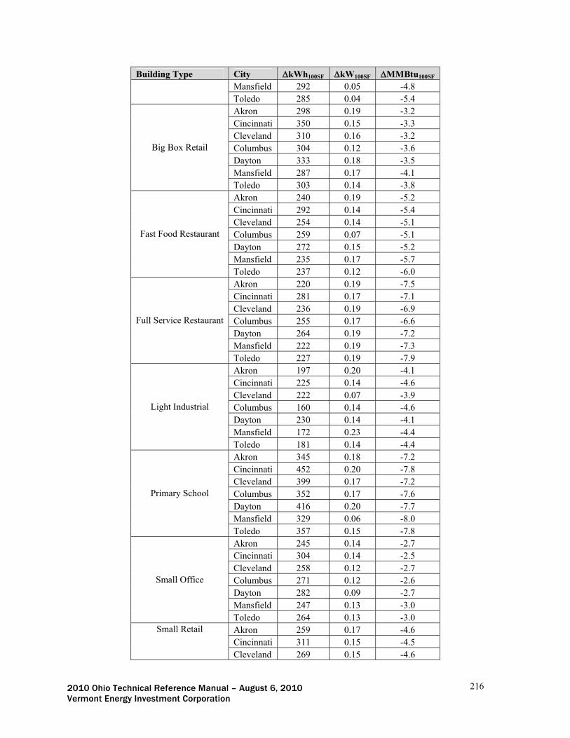
2010 Ohio Technical Reference Manual – August 6, 2010 216 Vermont Energy Investment Corporation
Building Type City kWh100SF kW100SF MMBtu100SF Mansfield 292 0.05 -4.8 Toledo 285 0.04 -5.4 Akron 298 0.19 -3.2 Cincinnati 350 0.15 -3.3 Cleveland 310 0.16 -3.2 Columbus 304 0.12 -3.6 Dayton 333 0.18 -3.5 Mansfield 287 0.17 -4.1
Big Box Retail
Toledo 303 0.14 -3.8 Akron 240 0.19 -5.2 Cincinnati 292 0.14 -5.4 Cleveland 254 0.14 -5.1 Columbus 259 0.07 -5.1 Dayton 272 0.15 -5.2 Mansfield 235 0.17 -5.7
Fast Food Restaurant
Toledo 237 0.12 -6.0 Akron 220 0.19 -7.5 Cincinnati 281 0.17 -7.1 Cleveland 236 0.19 -6.9 Columbus 255 0.17 -6.6 Dayton 264 0.19 -7.2 Mansfield 222 0.19 -7.3
Full Service Restaurant
Toledo 227 0.19 -7.9 Akron 197 0.20 -4.1 Cincinnati 225 0.14 -4.6 Cleveland 222 0.07 -3.9 Columbus 160 0.14 -4.6 Dayton 230 0.14 -4.1 Mansfield 172 0.23 -4.4
Light Industrial
Toledo 181 0.14 -4.4 Akron 345 0.18 -7.2 Cincinnati 452 0.20 -7.8 Cleveland 399 0.17 -7.2 Columbus 352 0.17 -7.6 Dayton 416 0.20 -7.7 Mansfield 329 0.06 -8.0
Primary School
Toledo 357 0.15 -7.8 Akron 245 0.14 -2.7 Cincinnati 304 0.14 -2.5 Cleveland 258 0.12 -2.7 Columbus 271 0.12 -2.6 Dayton 282 0.09 -2.7 Mansfield 247 0.13 -3.0
Small Office
Toledo 264 0.13 -3.0 Akron 259 0.17 -4.6 Cincinnati 311 0.15 -4.5
Small Retail
Cleveland 269 0.15 -4.6

2010 Ohio Technical Reference Manual – August 6, 2010 217 Vermont Energy Investment Corporation
Building Type City kWh100SF kW100SF MMBtu100SF Columbus 277 0.14 -4.6 Dayton 286 0.18 -4.9 Mansfield 252 0.18 -5.1 Toledo 262 0.16 -5.3
Version Date & Revision History Draft: Portfolio # Effective date: Date TRM will become effective End date: TBD

2010 Ohio Technical Reference Manual – August 6, 2010 218 Vermont Energy Investment Corporation
Roof Insulation (Retrofit – New Equipment) Official Measure Code (Measure Number: X-X-X-X (Efficient Products, Lighting End Use) Description This section covers improvements to the roof insulation in commercial buildings. Roof insulation R-value is assumed to increase to R-18 from the baseline level assumed for each building type. Energy and demand saving are realized through reductions in the building heating and cooling loads. The approach utilizes DOE-2.2 simulations on a series of commercial prototypical building models. The commercial simulation models are adapted from the California Database for Energy Efficiency Resources (DEER) study, with changes to reflect Ohio climate and building practices. Energy and demand impacts are normalized per thousand square feet of installed insulation. Definition of Efficient Equipment The efficient condition is R-18 insulation on the roof. Definition of Baseline Equipment The baseline condition by building type is shown in the table below:
Building Type Baseline R-Value Assembly R-12 Big Box Retail R-13.5 Fast Food R-13.5 Full Service Restaurant R-13.5 Light Industrial R-12 School R-13.5 Small Office R-13.5 Small Retail R-13.5
Deemed Calculation for this Measure
Annual kWh Savings = SF / 1000 * kWhkSF Summer Coincident Peak kW Savings = SF / 1000 * kWkSF * 0.74
Annual MMBtu Increase = SF / 1000 * MMBtukSF Deemed Lifetime of Efficient Equipment The expected lifetime of the measure is 20 years529. Deemed Measure Cost The full installed cost for retrofit applications is $1.36 per square foot530. Deemed O&M Cost Adjustments There are no expected O&M cost adjustments for this measure. Coincidence Factor The coincidence factor is 0.74531.
529 2008 Database for Energy-Efficiency Resources (DEER), Version 2008.2.05, “Effective/Remaining Useful Life Values”, California Public Utilities Commission, December 16, 2008. 530 2008 Database for Energy-Efficiency Resources (DEER), Version 2008.2.05, “Cost Values and Summary Documentation”, California Public Utilities Commission, December 16, 2008. 531 Coincidence factor supplied by Duke Energy for the commercial HVAC end-use. Pending verification based on information from the utilities.

2010 Ohio Technical Reference Manual – August 6, 2010 219 Vermont Energy Investment Corporation
REFERENCE SECTION
Calculation of Savings Energy Savings
ΔkWh = SF / 1000 * kWhkSF
Where:
SF = The square footage of the roof. To be collected with the incentive form. kWhkSF = the kWh savings per thousand square feet of roof area. This depends on the building
type and region in Ohio, and can be found in the lookup table below. Summer Coincident Peak Demand Savings
ΔkW = SF / 1000 * kWkSF * CF
Where:
kWkSF = the kW savings per thousand square feet of roof area. This depends on the building type and region in Ohio, and can be found in the lookup table below.
CF = The summer coincident peak factor, or 0.74. Baseline Adjustment There are no expected future code changes to affect this measure. Fossil Fuel Impact Descriptions and Calculation MMBtu = SF / 1000 * MMBtukSF Where:
MMBtukSF = unit gas savings per thousand square feet of roof space. See lookup table below.
Deemed O&M Cost Adjustment Calculation There are no expected O&M costs or savings associated with this measure. Reference Tables
Roof Insulation532 Building Type City kWhkSF KWkSF MMBtukSF
Akron 28 0.047 3.5 Cincinnati 34 0.065 2.7 Cleveland 26 0.021 2.9 Columbus 36 0.024 3.2 Dayton 36 0.076 3.5 Mansfield 31 0.012 3.3
Assembly
Toledo 41 0.018 5.0 532 Unit energy, demand, and gas savings data is based on a series of prototypical small commercial building simulation runs. The prototypes are based on the California DEER study prototypes, modified for local construction practices. Simulations were run using TMY3 weather data for each of the cities listed. Building prototypes used in the energy modeling are described in Appendix A - Prototypical Building Energy Simulation Model Development.

2010 Ohio Technical Reference Manual – August 6, 2010 220 Vermont Energy Investment Corporation
Building Type City kWhkSF KWkSF MMBtukSF Akron -6 0.025 2.5 Cincinnati -5 0.039 1.9 Cleveland -4 0.028 2.5 Columbus -1 0.034 2.6 Dayton -2 0.032 2.5 Mansfield -8 0.030 2.8
Big Box Retail
Toledo 2 0.023 3.0 Akron 37 0.050 3.6 Cincinnati 49 0.000 3.1 Cleveland 43 0.000 3.6 Columbus 39 0.000 3.3 Dayton 45 0.050 3.4 Mansfield 36 0.050 3.7
Fast Food Restaurant
Toledo 43 0.000 3.8 Akron 74 0.050 5.1 Cincinnati 77 0.050 4.3 Cleveland 78 0.025 5.3 Columbus 63 0.050 4.3 Dayton 69 0.075 4.4 Mansfield 71 0.050 5.3
Full-Service Restaurant
Toledo 84 0.050 5.6 Akron 57 0.028 4.3 Cincinnati 68 0.018 3.6 Cleveland 64 0.012 4.2 Columbus 51 0.023 3.6 Dayton 63 0.028 4.1 Mansfield 60 0.029 4.5
Light Industrial
Toledo 53 0.021 4.4 Akron 115 -0.008 4.4 Cincinnati 131 0.150 3.9 Cleveland 117 0.106 4.4 Columbus 109 0.054 4.0 Dayton 126 0.034 4.2 Mansfield 113 0.056 4.7
Primary School
Toledo 116 0.108 4.6 Akron 21 0.020 2.1 Cincinnati 26 0.040 1.6 Cleveland 27 0.020 2.1 Columbus 21 0.040 1.7 Dayton 26 0.000 1.9 Mansfield 20 0.040 2.2
Small Office
Toledo 23 0.020 2.1 Akron 51 0.047 3.4 Cincinnati 52 0.047 2.8 Cleveland 53 0.031 3.4 Columbus 43 0.031 2.9
Small Retail
Dayton 53 0.047 3.2

2010 Ohio Technical Reference Manual – August 6, 2010 221 Vermont Energy Investment Corporation
Building Type City kWhkSF KWkSF MMBtukSF Mansfield 48 0.047 3.6 Toledo 52 0.031 3.8
Version Date & Revision History Draft: Portfolio # Effective date: Date TRM will become effective End date: Date TRM will cease to be effective (or TBD)

2010 Ohio Technical Reference Manual – August 6, 2010 222 Vermont Energy Investment Corporation
High Performance Glazing (Retrofit – Early Replacement) Official Measure Code (Measure Number: X-X-X-X (Efficient Products, Lighting End Use) Description This section covers installation of high performance glazing in commercial buildings. The baseline condition is assumed to be double pane clear glass with a solar heat gain coefficient of 0.73 and U-value of 0.72 Btu/hr-SF-deg F. The efficient glazing must have a solar heat gain coefficient of 0.40 or less and U-value of 0.57 Btu/hr-SF-deg F or less. Energy and demand saving are realized through reductions in the building heating and cooling loads. The approach utilizes DOE-2.2 simulations on a series of commercial prototypical building models. The commercial simulation models are adapted from the California Database for Energy Efficiency Resources (DEER) study, with changes to reflect Ohio climate and building practices. Energy and demand impacts are normalized per 100 square feet of window. Definition of Efficient Equipment The efficient condition is a window with a U-value of 0.57 and a solar heat gain coefficient of 0.4. Definition of Baseline Equipment The baseline condition is a window with a U-value of 0.72 and a solar heat gain coefficient of 0.73. Deemed Calculation for this Measure
Annual kWh Savings = SF / 100 * (kWh100SF) Summer Coincident Peak kW Savings = SF / 100 * (kW100SF) * 0.74 Annual MMBTU Increase = SF / 100 * (MMBtu100SF)
Deemed Lifetime of Efficient Equipment The expected lifetime of the measure is 20 years533 . Deemed Measure Cost The full installed cost for retrofit applications is $54.82 per square foot of window534. Deemed O&M Cost Adjustments There are no expected O&M cost adjustments for this measure. Coincidence Factor The coincidence factor is 0.74535.
REFERENCE SECTION
Calculation of Savings
533 2008 Database for Energy-Efficiency Resources (DEER), Version 2008.2.05, “Effective/Remaining Useful Life Values”, California Public Utilities Commission, December 16, 2008. 534 Efficiency Vermont Technical Reference User Manual (TRM) Measure Savings Algorithms and Cost Assumptions, February, 19, 2010. Value derived from Efficiency Vermont project experience and conversations with suppliers. 535 Coincidence factor supplied by Duke Energy for the commercial HVAC end-use. Pending verification based on information from the utilities.

2010 Ohio Technical Reference Manual – August 6, 2010 223 Vermont Energy Investment Corporation
Energy Savings ΔkWh = SF / 100 * (kWh100SF)
Where:
SF = glazing surface area of installed window, not including frame (square feet). kWh100SF = the kWh savings per 100 square feet of window space. See lookup table
below. Summer Coincident Peak Demand Savings
ΔkW = SF / 100 * (kW100SF) * CF
Where:
kW100SF = the kW savings per 100 square feet of window space. See lookup table below. CF = The summer coincident peak factor, or 0.74.
Baseline Adjustment There are no expected future code changes to affect this measure. Fossil Fuel Impact Descriptions and Calculation ΔMMBtu = SF / 100 * (MMBtu100SF) Where:
MMBtu100SF = unit gas savings per 100 square feet of window space. See lookup table below.
Deemed O&M Cost Adjustment Calculation There are no expected O&M costs or savings associated with this measure. Reference Tables
High Performance Windows536 Building Type City ΔkWh100SF ΔkW100SF ΔMMBtu100SF
Akron 269 0.152 -0.28 Cincinnati 358 0.138 -0.86 Cleveland 300 0.143 -0.75 Columbus 278 0.052 -0.63 Dayton 312 0.157 -0.43 Mansfield 262 0.052 -0.26
Assembly
Toledo 264 0.038 -0.03 Akron 267 0.203 -0.35 Cincinnati 315 0.158 -1.23 Cleveland 281 0.169 -0.51 Columbus 278 0.124 -0.91 Dayton 301 0.180 -1.04
Big Box Retail
Mansfield 263 0.180 -0.56
536 Unit energy, demand, and gas savings data is based on a series of prototypical small commercial building simulation runs. The prototypes are based on the California DEER study prototypes, modified for local construction practices. Simulations were run using TMY3 weather data for each of the cities listed. Building prototypes used in the energy modeling are described in Appendix A - Prototypical Building Energy Simulation Model Development.

2010 Ohio Technical Reference Manual – August 6, 2010 224 Vermont Energy Investment Corporation
Building Type City ΔkWh100SF ΔkW100SF ΔMMBtu100SF Toledo 276 0.135 -0.59 Akron 253 0.189 -0.29 Cincinnati 301 0.155 -0.84 Cleveland 269 0.138 -0.31 Columbus 260 0.069 -0.86 Dayton 280 0.155 -0.65 Mansfield 251 0.172 -0.43
Fast Food Restaurant
Toledo 253 0.120 -0.79 Akron 268 0.193 -0.55 Cincinnati 313 0.166 -1.30 Cleveland 281 0.193 -0.47 Columbus 265 0.166 -1.63 Dayton 294 0.193 -1.22 Mansfield 259 0.193 -0.86
Full-Service Restaurant
Toledo 273 0.193 -1.02 Akron 218 0.136 -2.21 Cincinnati 188 0.203 -1.47 Cleveland 220 0.068 -1.40 Columbus 159 0.136 -2.21 Dayton 236 0.136 -1.47 Mansfield 186 0.226 -1.56
Light Industrial
Toledo 185 0.136 -1.81 Akron 398 0.189 -2.53 Cincinnati 493 0.204 -3.50 Cleveland 443 0.181 -2.63 Columbus 386 0.172 -3.41 Dayton 456 0.198 -3.35 Mansfield 384 0.065 -3.10
Primary School
Toledo 400 0.157 -3.08 Akron 241 0.144 -0.38 Cincinnati 294 0.144 -0.60 Cleveland 257 0.122 -0.41 Columbus 259 0.118 -0.68 Dayton 273 0.083 -0.52 Mansfield 241 0.131 -0.52
Small Office
Toledo 258 0.127 -0.59 Akron 272 0.177 -0.77 Cincinnati 315 0.158 -1.32 Cleveland 283 0.158 -0.75 Columbus 277 0.149 -1.42 Dayton 296 0.177 -1.23 Mansfield 266 0.186 -0.95
Small Retail
Toledo 274 0.158 -1.28

2010 Ohio Technical Reference Manual – August 6, 2010 225 Vermont Energy Investment Corporation
Version Date & Revision History Draft: Portfolio # Effective date: Date TRM will become effective End date: Date TRM will cease to be effective (or TBD)
2010 Ohio Technical Reference Manual – August 6, 2010 226 Vermont Energy Investment Corporation
Engineered Nozzles (Time of Sale, Retrofit - Early Replacement) Official Measure Code (Measure Number: X-X-X-X (Program name, End Use) Description Engineered nozzles use compressed air to entrain and amplify atmospheric air into a stream, thus increasing pressure with minimal compressed air use. They are able to induce a large airflow entrainment while still using a smaller volume of air than open jets. The velocity of the resulting airflow is reduced, but the mass flow of the air is increased, thus increasing the cooling and drying effect. Energy savings result due to a decrease in compressor work that is required to provide the nozzles with compressed air. Engineered nozzles have the added benefits of noise reduction and improved safety in systems with greater than 30 psig. Definition of Efficient Equipment The efficient condition assumes an engineered nozzle is equipped to the end of a pneumatic tool. Definition of Baseline Equipment The baseline condition assumes an open copper tube or an air gun with an open end. Deemed Savings for this Measure
Annual kWh Savings = 0.0145 x (FLOWbaseline - FLOWeng) X HOURS
Summer Coincident Peak kW Savings = 0.0109 x (FLOWbaseline - FLOWeng)
Deemed Lifetime of Efficient Equipment 15 years537 Deemed Measure Cost $14538 Deemed O&M Cost Adjustments n/a Coincidence Factor 0.75539
REFERENCE SECTION
Calculation of Savings Energy Savings
ΔkWh = (FLOWbaseline - FLOWeng) x kWscfm x %USE x HOURS
Where: kWscfm = the average amount of electrical demand needed to produce one cubic foot of air at 100
PSI = 0.29540
537 PA Consulting Group (2009). Business Programs: Measure Life Study. Prepared for State of Wisconsin Public Service Commission 538 See “Compressed Air Analysis.xls” for cost details 539 PG&E 1996, RLW Schools, RLW CF, SDG&E Time of Use Surveys. Based on 4p-5p peak 540 See “Compressed Air Analysis.xls” for more detail

2010 Ohio Technical Reference Manual – August 6, 2010 227 Vermont Energy Investment Corporation
FLOWbaseline = The flow rate of compressed air from an open end (SCFM) FLOWeng = The flow rate of compressed air from an engineered nozzle (SCFM)
= Depending on size of nozzle:
Open Flow (SCFM)541 FLOWbaseline
Engineered Nozzle (SCFM)542 FLOWeng
ΔSCFM
1/8" Nozzle 21 6 15
1/4" Nozzle 58 11 47
%USE = percent of the compressor total operating hours that the nozzle is in use (5% for 3
seconds of use per minute) = 0.05543
HOURS = annual operating hours of the compressed air system = If site specific value is unknown, assume vales based on number of facility shifts as
below:
No. of Shifts HOURS Description Single Shift(8/5) 1976 7am – 3pm, weekdays, minus holidays and scheduled downtime 2-Shift 3952 7am – 11pm, weekdays, minus holidays and scheduled downtime 3-Shift 5928 24 hours per day, weekdays, minus holidays and scheduled downtime 4-Shift 8320 24 hours per day, 7 days a week minus holidays and scheduled downtime
Summer Coincident Peak Demand Savings
ΔkW = ΔkWh / HOURS x CF
Where:
ΔkWh = Energy Savings, caculated above
HOURS = Operating Hours, see above CF = Peak coincidence factor = 0.75 Fossil Fuel Impact Descriptions and Calculation n/a Water Impact Descriptions and Calculation n/a Deemed O&M Cost Adjustment Calculation n/a Version Date & Revision History Draft: Portfolio # Effective date: Date TRM will become effective End date: Date TRM will cease to be effective (or TBD)
541 Machinery’s Handbook 25th Edition. 542 Survey of Engineered Nozzle Suppliers 543 Assumes 50% handheld air guns and 50% stationary air nozzles. Manual air guns tend to be used less than stationary air nozzles, and a conservative estimate of 1 second of blow-off per minute of compressor run time is assumed. Stationary air nozzles are commonly more wasteful as they are often mounted on machine tools and can be manually operated resulting in the possibility of a long term open blow situation. An assumption of 5 seconds of blow-off per minute of compressor run time is used.
2010 Ohio Technical Reference Manual – August 6, 2010 228 Vermont Energy Investment Corporation
Insulated Pellet Dryers (Retrofit) Official Measure Code (Measure Number: X-X-X-X (Program name, End Use) Description Resin pellets used in injection molders and extruders are typically dried using electrically heated and desiccant dried air. Flexible ducts in the 3” to 8” diameter size range circulate the drying air. Air temperatures usually range from 160°F to 200°F. Un-insulated duct heat loss must be replaced by electric resistance heaters. Most facilities have pellet dryers running constantly to maintain pellet dryness at all times. Definition of Efficient Equipment The efficient condition is a pellet dryer with insulation on the heat ducts. Definition of Baseline Equipment The baseline condition is pellet dryer with un-insulated heat ducts.
Deemed Savings for this Measure
Annual kWh Savings = L x (kWbaseline-kWeff) x HOURS Summer Coincident Peak kW Savings = L x (kWbaseline-kWeff) x CF
Deemed Lifetime of Efficient Equipment 5 years544 Deemed Measure Cost Incremental costs are based on linear feet and diameter of heating ducts.
Incremental Capital Cost545
Diameter of Pipe (in.) Incremental Cost of
Insulation ($/ft.) 3” $33
4” $43
5” $54
6” $65
8” $86 Deemed O&M Cost Adjustments n/a Coincidence Factor 0.75546
REFERENCE SECTION
Calculation of Savings
544 Engineering Judgment 545 Based on a review of available manufacturer pricing information 546 PG&E 1996, RLW Schools, RLW CF, SDG&E Time of Use Surveys.
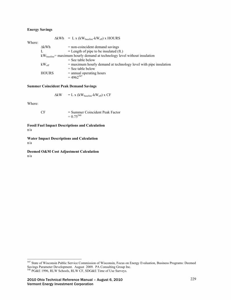
2010 Ohio Technical Reference Manual – August 6, 2010 229 Vermont Energy Investment Corporation
Energy Savings ∆kWh = L x (kWbaseline-kWeff) x HOURS
Where: ∆kWh = non-coincident demand savings
L = Length of pipe to be insulated (ft.) kWbaseline = maximum hourly demand at technology level without insulation = See table below kWeff = maximum hourly demand at technology level with pipe insulation = See table below
HOURS = annual operating hours = 4962547
Summer Coincident Peak Demand Savings
∆kW = L x (kWbaseline-kWeff) x CF
Where:
CF = Summer Coincident Peak Factor = 0.75548 Fossil Fuel Impact Descriptions and Calculation n/a Water Impact Descriptions and Calculation n/a Deemed O&M Cost Adjustment Calculation n/a
547 State of Wisconsin Public Service Commission of Wisconsin, Focus on Energy Evaluation, Business Programs: Deemed Savings Parameter Development. August 2009. PA Consulting Group Inc. 548 PG&E 1996, RLW Schools, RLW CF, SDG&E Time of Use Surveys.

2010 Ohio Technical Reference Manual – August 6, 2010 230 Vermont Energy Investment Corporation
Reference Tables
Electric Demand for Load Temperatures and Duct Diameters Temperature
(°F) Duct Diameter (in) KWbaseline KWenergyefficientmethod ΔKW
3 0.03/ft 0.01/ft 0.02/ft4 0.04/ft 0.01/ft 0.03/ft5 0.05/ft 0.01/ft 0.04/ft6 0.06/ft 0.01/ft 0.05/ft
8 0.09/ft 0.01/ft 0.08/ft
3 0.03/ft 0.01/ft 0.03/ft4 0.05/ft 0.01/ft 0.04/ft5 0.06/ft 0.01/ft 0.05/ft6 0.07/ft 0.01/ft 0.06/ft8 0.10/ft 0.01/ft 0.09/ft3 0.04/ft 0.01/ft 0.03/ft4 0.05/ft 0.01/ft 0.04/ft5 0.07/ft 0.01/ft 0.06/ft6 0.08/ft 0.01/ft 0.07/ft8 0.11/ft 0.01/ft 0.10/ft3 0.04/ft 0.01/ft 0.04/ft4 0.06/ft 0.01/ft 0.05/ft5 0.07/ft 0.01/ft 0.06/ft6 0.09/ft 0.01/ft 0.08/ft8 0.13/ft 0.02/ft 0.11/ft3 0.05/ft 0.01/ft 0.04/ft4 0.07/ft 0.01/ft 0.06/ft5 0.08/ft 0.01/ft 0.07/ft6 0.10/ft 0.01/ft 0.09/ft8 0.14/ft 0.02/ft 0.12/ft
160
170
180
190
200
Version Date & Revision History Draft: Portfolio # Effective date: Date TRM will become effective End date: Date TRM will cease to be effective (or TBD)

2010 Ohio Technical Reference Manual – August 6, 2010 231 Vermont Energy Investment Corporation
Injecting Molding Barrel Wrap (Retrofit – New Equipment) Official Measure Code (Measure Number: X-X-X-X (Program name, End Use) Description Removable insulated blankets enclose the cylindrical barrels of an injection molding machine. Surface temperatures of the barrels range from 300°F to 600°F, depending on the resins processed. Barrels are heated either with electric resistance band heaters or by friction from the mechanical screw which shears plastic material in the barrel generating frictional heat. Insulated blankets minimize the use of resistance heating without affecting temperature control of the resin. Barrel wraps are held in place by straps. Blankets are available either in standard sizes or can be custom manufactured. Definition of Efficient Equipment The efficient condition is assumed to be an injection molding machine with an insulating blanket or vest wrapped around the barrel. Definition of Baseline Equipment The baseline condition is assumed to be an injection molding machine with no added insulation.
Deemed Savings for this Measure
Annual kWh Savings = (ΔELoss * LENBarrel * DBarrel * π) / 1000 * HOURS Summer Coincident Peak kW Savings = (ΔELoss * LENBarrel * DBarrel * π) / 1000
Deemed Lifetime of Efficient Equipment 5 years549 Deemed Measure Cost The actual measure installation cost should be used (including material and labor). Deemed O&M Cost Adjustments n/a Coincidence Factor 0.75550
REFERENCE SECTION
Calculation of Savings Energy Savings
ΔkWh = (ΔELoss * LENBarrel * DBarrel * π) / 1000 * HOURS Where:
ΔELoss = The difference in heat loss (measured in watts/ft2 needed to replace lost heat) between an injection molding barrel with insulation compared to an injection molding barrel without insulation. This is dependent on the operating temperatiure (site specific) and the
549 Engineering judgment 550 PG&E 1996, RLW Schools, RLW CF, SDG&E Time of Use Surveys. Pending verification based on information to be provided by the utilities.

2010 Ohio Technical Reference Manual – August 6, 2010 232 Vermont Energy Investment Corporation
thickness of the insulation (site specific). See the table “Calculating Barrel Heat Loss” in the reference table section for associated values.
LENBarrel = The length of the barrel = Actual installed
DBarrel = The diameter of the barrel = Actual installed π = 3.14159 1000 = conversion factor for watts to kilowatts
HOURS = Annual operating hours = If actual operating hours are unknown, assume 3952551.
Summer Coincident Peak Demand Savings
ΔkW = (ΔELoss * LENBarrel * DBarrel * π) / 1000 * CF
Where: CF = Summer Peak Coincidence Factor = 0.75 Fossil Fuel Impact Descriptions and Calculation n/a Water Impact Descriptions and Calculation n/a Deemed O&M Cost Adjustment Calculation n/a Reference Tables
Calculating Barrel Heat Loss552
Operating Temperature
(°F) No Insulation
(Watts/ ft2) 1” Insulation
(Watts/ft2) 1.5” Insulation
(Watts/ft2) 300 180 18.6 12.4 325 210 20.9 14 350 243 23.4 15.6 375 275 26 17.3 400 313 29 19 425 350 31.5 21 450 387 34.3 22.9 475 425 37.2 24.8 500 465 40.1 25.8 525 505 43.2 26.9 550 550 46.5 28.3 575 605 49.9 29.9 600 660 54.1 32.1
551 Default annual operating hours estimate assumes equipment operates continuously on a typical 2-shift operation (7am – 11pm, weekdays, minus some holidays and scheduled down time). 552 Industrial Modeling Supplies (2009). Reference/Conversion Chart. http://www.imscompany.com/pdf/Tech%20Tips%20&%20Conversion%20and%20Reference%20Charts.pdf

2010 Ohio Technical Reference Manual – August 6, 2010 233 Vermont Energy Investment Corporation
Version Date & Revision History Draft: Portfolio # Effective date: Date TRM will become effective End date: Date TRM will cease to be effective (or TBD)
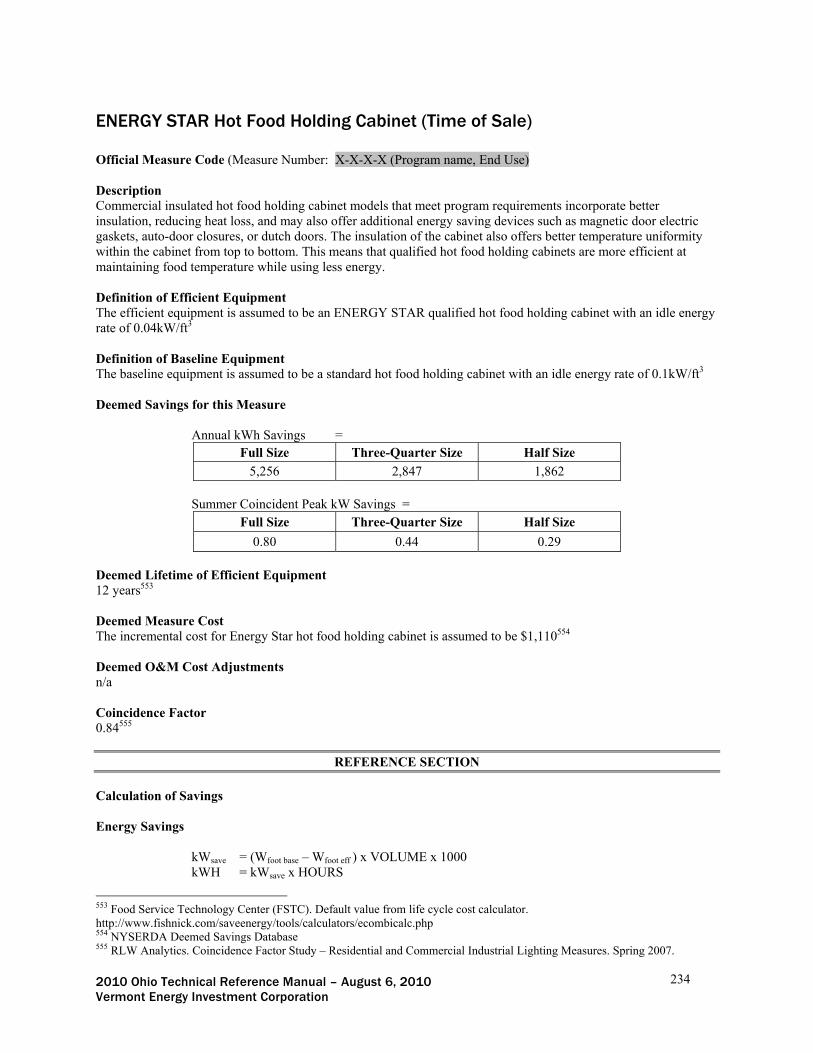
2010 Ohio Technical Reference Manual – August 6, 2010 234 Vermont Energy Investment Corporation
ENERGY STAR Hot Food Holding Cabinet (Time of Sale) Official Measure Code (Measure Number: X-X-X-X (Program name, End Use) Description Commercial insulated hot food holding cabinet models that meet program requirements incorporate better insulation, reducing heat loss, and may also offer additional energy saving devices such as magnetic door electric gaskets, auto-door closures, or dutch doors. The insulation of the cabinet also offers better temperature uniformity within the cabinet from top to bottom. This means that qualified hot food holding cabinets are more efficient at maintaining food temperature while using less energy. Definition of Efficient Equipment The efficient equipment is assumed to be an ENERGY STAR qualified hot food holding cabinet with an idle energy rate of 0.04kW/ft3 Definition of Baseline Equipment The baseline equipment is assumed to be a standard hot food holding cabinet with an idle energy rate of 0.1kW/ft3
Deemed Savings for this Measure
Annual kWh Savings =
Full Size Three-Quarter Size Half Size
5,256 2,847 1,862
Summer Coincident Peak kW Savings = Full Size Three-Quarter Size Half Size
0.80 0.44 0.29
Deemed Lifetime of Efficient Equipment 12 years553 Deemed Measure Cost The incremental cost for Energy Star hot food holding cabinet is assumed to be $1,110554 Deemed O&M Cost Adjustments n/a Coincidence Factor 0.84555
REFERENCE SECTION
Calculation of Savings Energy Savings
kWsave = (Wfoot base – Wfoot eff ) x VOLUME x 1000 kWH = kWsave x HOURS
553 Food Service Technology Center (FSTC). Default value from life cycle cost calculator. http://www.fishnick.com/saveenergy/tools/calculators/ecombicalc.php 554 NYSERDA Deemed Savings Database 555 RLW Analytics. Coincidence Factor Study – Residential and Commercial Industrial Lighting Measures. Spring 2007.

2010 Ohio Technical Reference Manual – August 6, 2010 235 Vermont Energy Investment Corporation
Where:
kWsave = the difference in connected load between the baseline and the efficient equipment (before the coincidence factor is applied)
HOURS = Annual operating hours = 5475556
Summer Coincident Peak Demand Savings
kWsave = (Wfoot base – Wfoot eff ) x VOLUME x 1000
ΔkW = kW x CF
Where:
kWsave = the difference in connected load between the baseline and the efficient equipment (before the coincidence factor is applied)
Wfoot base = the electrical demand per cubic foot of the baseline equpiment Wfoot eff = the electrical demand per cubic foot of the efficient equipment VOLUME = the internal volume of the holding cabinet (ft3) 1,000 = conversion of W to kW
Parameter Full Size Three-Quarter
Size Half Size VOLUME557 20 12 8 Wfoot base 70 70 70 Wfoot eff 22 27 29 kWsave 0.96 0.52 0.34
CF = Summer Peak Coincidence Factor = 0.84 Fossil Fuel Impact Descriptions and Calculation n/a Water Impact Descriptions and Calculation n/a Deemed O&M Cost Adjustment Calculation n/a Reference Tables n/a Version Date & Revision History Draft: Portfolio # Effective date: Date TRM will become effective End date: Date TRM will cease to be effective (or TBD)
556 Food Service Technology Center (FSTC), based on assumption that restaurant is open 15 hours a day, 365 days a year. 557 Sizes are from ENERGY STAR calculator

2010 Ohio Technical Reference Manual – August 6, 2010 236 Vermont Energy Investment Corporation
Steam Cookers (Time of Sale) Official Measure Code (Measure Number: X-X-X-X (Program name, End Use) Description Energy efficient steam cookers that have earned the ENERGY STAR offer shorter cook times, higher production rates, and reduced heat loss due to better insulation and more efficient steam delivery system. Energy usage calculations are based on 12 hours a day, 365 days per year, with one preheat and cooking 100 pounds per day of food. Definition of Efficient Equipment The efficient condition assumes the installation of an ENERGY STAR qualified steam cooker. Definition of Baseline Equipment The baseline condition assumes a conventional boiler-style steam cooker meeting minimum federal standards for electricity and water consumption. Deemed Calculations for this Measure
Annual kWh Savings = kWHbase - kWheff
Summer Coincident Peak kW Savings = (Annual kWh Savings / HOURS) x CF
Deemed Lifetime of Efficient Equipment 12 years558 Deemed Measure Cost The incremental cost of an ENERGY STAR steam cooker is $2,000559 Deemed O&M Cost Adjustments n/a Coincidence Factor 0.84560
REFERENCE SECTION
Calculation of Savings Energy Savings
kWH = [LB x EFOOD/EFF + IDLE x (HOURSDAY – LB/PC – PRETIME /60) + PREENERGY] x DAYS ΔkWh = kWHbase - kWheff
Where:
kWHbase = the annual energy usage of the baseline equipment calculated using baseline values kWHeff = the annual energy usage of the efficient equipment calculated using efficient values HOURSDAY = Daily operating hours
558 Food Service Technology Center (FSTC). Default value from life cycle cost calculator. http://www.fishnick.com/saveenergy/tools/calculators/esteamercalc.php 559 NYSERDA Deemed Savings Database 560 RLW Analytics. Coincidence Factor Study – Residential and Commercial Industrial Lighting Measures. Spring 2007.

2010 Ohio Technical Reference Manual – August 6, 2010 237 Vermont Energy Investment Corporation
= 12561 PRETIME = Preheat time (min/day), the amount of time it takes a steamer to reach operating
temperature when turned on = 15 min/day562 PREENERGY = Preheat energy (kWh/day) = 1.5 kWh/day563 EFOOD = ASTM Energy to Food (kWh/lb); the amount of energy absorbed by the food during
cooking, per pound of food = 0.038564 DAYS = Operating days per year = 365 The following variables are dependent on the pan capacity of efficient equipment which is a site specific variable. See the ‘Reference Tables’ section for the associated values EFF = Heavy load cooking energy efficiency (%) IDLE = Idle energy rate PC = Production capacity (lbs/hr) LB = Pounds of food cooked per day (lb/day)
Summer Coincident Peak Demand Savings
ΔkW = (ΔkWh / HOURS) x CF
Where:
ΔkWh = Annual energy savings (kWh) HOURS = Equivalent full load hours
= 4380 CF = Summer Peak Coincidence Factor for measure
= 0.84 Fossil Fuel Impact Descriptions and Calculation n/a Water Impact Descriptions and Calculation ΔWater = (Ratebase – Rateeff) x EFLH = 30 x EFLH Where ΔWater = Annual water savings (gal) Ratebase = Water consumption rate (gal/h) of baseline equipment = 40565 Rateeff = Water consumption rate (gal/h) of baseline equipment = 10566 EFLH = Equivalent full load hours = 4380
561 Food Service Technology Center (FSTC), based on assumption that restaurant is open 12 hours a day, 365 days a year. 562 FSTC (2002). Commercial Cooking Appliance Technology Assessment. Chapter 8: Steamers. 563 Ibid. 564 American Society for Testing and Materials. Industry Standard. 565 FSTC (2002). Commercial Cooking Appliance Technology Assessment. Chapter 8: Steamers. 566 Ibid.

2010 Ohio Technical Reference Manual – August 6, 2010 238 Vermont Energy Investment Corporation
Deemed O&M Cost Adjustment Calculation n/a Reference Tables Values for ASTM parameters for baseline and efficient conditions (unless otherwise noted) were determined by FSTC according to ASTM F1484, the Standard Test Method for Performance of Steam Cookers. These parameters include the three of the four listed below: Idle Energy Rate, Production Capacity, and Heavy Load Cooking Efficiency. Pounds of Food Cooked per Day based on the default value for a 3 pan steam cooker (100 lbs from FSTC) and scaled up based on the assumption that steam cookers with a greater number of pans cook larger quantities of food per day. It is not known which specific models were tested but the values presented are thought to be the averages of tested models. Parameters that vary with number of pans: # of Pans Parameter Baseline Model Efficient Model
Idle Energy Rate (kW)567 1 0.24 Production Capacity (lb/h) 70 50 Pounds of Food Cooked per Day 100 100
3
Heavy Load Cooking Energy Efficiency568 20% 59% Idle Energy Rate (kW) 1.325 0.27 Production Capacity (lb/h) 87 67 Pounds of Food Cooked per Day 128 128
4
Heavy Load Cooking Energy Efficiency 20% 52% Idle Energy Rate (kW) 1.675 0.24 Production Capacity (lb/h) 103 83 Pounds of Food Cooked per Day 160 160
5
Heavy Load Cooking Energy Efficiency 20% 62% Idle Energy Rate (kW) 2 0.31 Production Capacity (lb/h) 120 100 Pounds of Food Cooked per Day 192 192
6
Heavy Load Cooking Energy Efficiency 20% 62% Version Date & Revision History Draft: Portfolio # Effective date: Date TRM will become effective End date: Date TRM will cease to be effective (or TBD)
567 Efficient values calculated from a list of ENERGY STAR qualified products. See “ES Steam Cooker Analysis.xls” for details. 568 Ibid.

2010 Ohio Technical Reference Manual – August 6, 2010 239 Vermont Energy Investment Corporation
ENERGY STAR Fryers (Time of Sale) Official Measure Code (Measure Number: X-X-X-X (Program name, End Use) Description Commercial fryers that have earned the ENERGY STAR offer shorter cook times and higher production rates through advanced burner and heat exchanger designs. Frypot insulation reduces standby losses resulting in a lower idle energy rate. Fryers that have earned the ENERGY STAR are up to 30% more efficient than standard models. Energy savings estimates are based on a 15” fryer. Definition of Efficient Equipment The efficient equipment is assumed to be an ENERGY STAR qualified electric fryer Definition of Baseline Equipment The baseline equipment is assumed to be a standard electric fryer with a heavy load efficiency of 75%. Deemed Savings for this Measure
Annual kWh Savings = 982.71 kWh/yr
Summer Coincident Peak kW Savings = 0.22 kW
Deemed Lifetime of Efficient Equipment 12 years569 Deemed Measure Cost The incremental cost for commercial combination ovens is assumed to be $500570 Deemed O&M Cost Adjustments n/a Coincidence Factor 0.84571
REFERENCE SECTION
Calculation of Savings Energy Savings
kWH = [LB x EFOOD/EFF + IDLE x (HOURSDAY – LB/PC – PRETIME /60) + PREENERGY] x DAYS ΔkWh = kWHbase - kWheff
Where:
kWHbase = the annual energy usage of the baseline equipment calculated using baseline values kWHeff = the annual energy usage of the efficient equipment calculated using efficient values HOURSDAY = Daily operating hours = 16572
569 Food Service Technology Center (FSTC). Default value from life cycle cost calculator. http://www.fishnick.com/saveenergy/tools/calculators/ecombicalc.php 570 NYSERDA Deemed Savings Database 571 RLW Analytics. Coincidence Factor Study – Residential and Commercial Industrial Lighting Measures. Spring 2007.

2010 Ohio Technical Reference Manual – August 6, 2010 240 Vermont Energy Investment Corporation
PRETIME = Preheat time (min/day), the amount of time it takes a fryer to reach operating temperature when turned on
= 15 min/day573 EFOOD = ASTM Energy to Food (kWh/lb); the amount of energy absorbed by the food during
cooking, per pound of food = 0.167574 LB = Pounds of food cooked per day (lb/day) = 150575 DAYS = 365 EFF = Heavy load cooking energy efficiency (%) IDLE = Idle energy rate PC = Production capacity (lbs/hr) PREENERGY = Preheat energy (kWh/day) Performance Metrics: Baseline and Efficient Values576
Metric Baseline Model Energy Efficient
Model PREENERGY 2.3 1.7 IDLE 1.05 0.84
EFF 75% 84% PC 65 70
Summer Coincident Peak Demand Savings
ΔkW = (ΔkWh / HOURS) x CF
Where:
ΔkWh = Annual energy savings (kWh) HOURS = Equivalent full load hours
= 4380 CF = Summer Peak Coincidence Factor for measure
= 0.84 Fossil Fuel Impact Descriptions and Calculation n/a Water Impact Descriptions and Calculation n/a Deemed O&M Cost Adjustment Calculation n/a Version Date & Revision History Draft: Portfolio # Effective date: Date TRM will become effective End date: Date TRM will cease to be effective (or TBD)
572 Food Service Technology Center (FSTC), based on assumption that restaurant is open 16 hours a day, 365 days a year. 573 FSTC (2002). Commercial Cooking Appliance Technology Assessment. Chapter 7: Fryers. 574 American Society for Testing and Materials. Industry Standard for Commercial Ovens. 575 Food Service Technology Center (FSTC). Default value from life cycle cost calculator. http://www.fishnick.com/saveenergy/tools/calculators/ecombicalc.php 576 Baseline values based on assumptions from FSTC life cycle cost calculator. Efficient values reflect averages from a list of qualifying models found on the ENERGY STAR website (accessed June 2010)

2010 Ohio Technical Reference Manual – August 6, 2010 241 Vermont Energy Investment Corporation
Combination Oven (Time of Sale) Official Measure Code (Measure Number: X-X-X-X (Program name, End Use) Description A combination oven is a convection oven that includes the added capability to inject steam into the oven cavity and typically offers at least three distinct cooking modes. Definition of Efficient Equipment The efficient equipment is assumed to be an electric combination oven with a heavy load cooking energy efficiency of at least 60%. Definition of Baseline Equipment The baseline equipment is assumed to be a typical low-efficiency oven with a heavy load efficiency of 44%. Deemed Savings for this Measure
Annual kWh Savings = 18,432 kWh
Summer Coincident Peak kW Savings = 3.53 kW
Deemed Lifetime of Efficient Equipment 12 years577 Deemed Measure Cost The incremental cost for commercial combination ovens is assumed to be $2,125578 Deemed O&M Cost Adjustments n/a Coincidence Factor 0.84579
REFERENCE SECTION
Calculation of Savings Energy Savings
kWH = [LB x EFOOD/EFF + IDLE x (HOURSDAY – LB/PC – PRETIME /60) + PREENERGY] x DAYS ΔkWh = kWHbase - kWheff
Where:
kWHbase = the annual energy usage of the baseline equipment calculated using baseline values kWHeff = the annual energy usage of the efficient equipment calculated using efficient values HOURSDAY = Daily operating hours = 12580
577 Food Service Technology Center (FSTC). Default value from life cycle cost calculator. http://www.fishnick.com/saveenergy/tools/calculators/ecombicalc.php 578 NYSERDA Deemed Savings Database 579 RLW Analytics. Coincidence Factor Study – Residential and Commercial Industrial Lighting Measures. Spring 2007. 580 Food Service Technology Center (FSTC), based on assumption that restaurant is open 12 hours a day, 365 days a year.

2010 Ohio Technical Reference Manual – August 6, 2010 242 Vermont Energy Investment Corporation
DAYS = Days per year of operation = 365 PRETIME = Preheat time (min/day), the amount of time it takes a steamer to reach operating
temperature when turned on = 15 min/day581 EFOOD = ASTM Energy to Food (kWh/lb); the amount of energy absorbed by the food during
cooking, per pound of food = 0.0732582 LB = Pounds of food cooked per day (lb/day) = 200583 EFF = Heavy load cooking energy efficiency (%) IDLE = Idle energy rate PC = Production capacity (lbs/hr) PREENERGY = Preheat energy (kWh/day) Performance Metrics: Baseline and Efficient Values584
Metric Baseline Model Energy Efficient
Model PREENERGY (kWh) 3 1.5 IDLE (kW) 7.5 3
EFF 44% 60% PC (lb/hr) 80 100
Summer Coincident Peak Demand Savings
ΔkW = (ΔkWh / HOURS) x CF
Where:
ΔkWh = Annual energy savings (kWh) HOURS = Equivalent full load hours
= 4380 CF = Summer Peak Coincidence Factor for measure
= 0.84 Fossil Fuel Impact Descriptions and Calculation n/a Water Impact Descriptions and Calculation The water savings for commercial combination ovens are assumed to be 87,600 gallons per year585 Deemed O&M Cost Adjustment Calculation n/a
581 Food Service Technology Center (2002). Commercial Cooking Appliance Technology Assessment. Prepared by Don Fisher.. Chapter 7: Ovens. 582 American Society for Testing and Materials. Industry Standard for Commercial Ovens. 583 Food Service Technology Center (FSTC). Default value from life cycle cost calculator. http://www.fishnick.com/saveenergy/tools/calculators/ecombicalc.php 584 Ibid. 585 Food Service Technology Center (FSTC). Based on assumption that baseline ovens use water at an average rate of 40 gal/h while efficient models use water at an average rate of 20 gal/h

2010 Ohio Technical Reference Manual – August 6, 2010 243 Vermont Energy Investment Corporation
Version Date & Revision History Draft: Portfolio # Effective date: Date TRM will become effective End date: Date TRM will cease to be effective (or TBD)

2010 Ohio Technical Reference Manual – August 6, 2010 244 Vermont Energy Investment Corporation
Convection Oven (Time of Sale) Official Measure Code (Measure Number: X-X-X-X (Program name, End Use) Description Commercial convection ovens that are ENERGY STAR certified have higher heavy load cooking efficiencies, and lower idle energy rates making them on average about 20 percent more efficient than standard models. Energy savings estimates are for ovens using full size (18” x 36”) sheet pans. Definition of Efficient Equipment The efficient equipment is assumed to be an ENERGY STAR qualified electric convection oven. Definition of Baseline Equipment The baseline equipment is assumed to be a standard convection oven with a heavy load efficiency of 65%. Deemed Savings for this Measure
Annual kWh Savings = 3,235 kWh
Summer Coincident Peak kW Savings = 0.62 kW
Deemed Lifetime of Efficient Equipment 12 years586 Deemed Measure Cost The incremental cost for commercial convection ovens is assumed to be $1,113587 Deemed O&M Cost Adjustments n/a Coincidence Factor 0.84588
REFERENCE SECTION
Calculation of Savings Energy Savings
kWH = [LB x EFOOD/EFF + IDLE x (HOURSDAY – LB/PC – PRETIME /60) + PREENERGY] x DAYS ΔkWh = kWHbase - kWheff
Where:
kWHbase = the annual energy usage of the baseline equipment calculated using baseline values kWHeff = the annual energy usage of the efficient equipment calculated using efficient values HOURSDAY = Daily operating hours = 12589
586 Food Service Technology Center (FSTC). Default value from life cycle cost calculator. http://www.fishnick.com/saveenergy/tools/calculators/ecombicalc.php 587 NYSERDA Deemed Savings Database 588 RLW Analytics. Coincidence Factor Study – Residential and Commercial Industrial Lighting Measures. Spring 2007. 589 Food Service Technology Center (FSTC), based on assumption that restaurant is open 12 hours a day, 365 days a year.

2010 Ohio Technical Reference Manual – August 6, 2010 245 Vermont Energy Investment Corporation
DAYS = Days per year of operation = 365 PRETIME = Preheat time (min/day), the amount of time it takes a steamer to reach operating
temperature when turned on = 15 min/day590 EFOOD = ASTM Energy to Food (kWh/lb); the amount of energy absorbed by the food during
cooking, per pound of food = 0.0732591 LB = Pounds of food cooked per day (lb/day) = 100592 EFF = Heavy load cooking energy efficiency (%). See table below. IDLE = Idle energy rate. See table below. PC = Production capacity (lbs/hr). See table below. PREENERGY = Preheat energy (kWh/day). See table below. Performance Metrics: Baseline and Efficient Values593
Metric Baseline Model Energy Efficient
Model PREENERGY (kWh) 1.5 1 IDLE (kW) 2 1.3594
EFF 65% 74%595 PC (lb/hr) 70 80
Summer Coincident Peak Demand Savings
ΔkW = (ΔkWh / HOURS) x CF
Where:
ΔkWh = Annual energy savings (kWh) HOURS = Equivalent full load hours
= 4380 CF = Summer Peak Coincidence Factor for measure
= 0.84 Fossil Fuel Impact Descriptions and Calculation n/a Water Impact Descriptions and Calculation n/a Deemed O&M Cost Adjustment Calculation n/a
590 Food Service Technology Center (2002). Commercial Cooking Appliance Technology Assessment. Prepared by Don Fisher.. Chapter 7: Ovens. 591 American Society for Testing and Materials. Industry Standard for Commercial Ovens. 592 Food Service Technology Center (FSTC). Default value from life cycle cost calculator. http://www.fishnick.com/saveenergy/tools/calculators/ecombicalc.php 593 Ibid. 594 Calculated from list of Energy Star qualified models, http://www.energystar.gov/ia/products/prod_lists/comm_ovens_prod_list.xls 595 Ibid.

2010 Ohio Technical Reference Manual – August 6, 2010 246 Vermont Energy Investment Corporation
Version Date & Revision History Draft: Portfolio # Effective date: Date TRM will become effective End date: Date TRM will cease to be effective (or TBD)

2010 Ohio Technical Reference Manual – August 6, 2010 247 Vermont Energy Investment Corporation
ENERGY STAR Griddle (Time of Sale) Official Measure Code (Measure Number: X-X-X-X (Program name, End Use) Description ENERGY STAR qualified commercial griddles have higher cooking energy efficiency and lower idle energy rates than standard equipment. The result is more energy being absorbed by the food compared with the total energy use, and less wasted energy when the griddle is in standby mode. Definition of Efficient Equipment The efficient equipment is assumed to be an ENERGY STAR qualified griddle that has a cooking energy efficiency greater than 70% Definition of Baseline Equipment The baseline equipment is assumed to be a conventional electric griddle with a cooking energy efficiency of 60% Deemed Calculations for this Measure
Annual kWh Savings = kWhbase - kWheff
Summer Coincident Peak kW Savings = (Annual kWh Savings / HOURS) x CF
Deemed Lifetime of Efficient Equipment 12 years596 Deemed Measure Cost The incremental cost of an ENERGY STAR griddle is assumed to be $2,090597. Deemed O&M Cost Adjustments n/a Coincidence Factor 0.84598
REFERENCE SECTION
Calculation of Savings Energy Savings
kWhi = [LB x EFOOD / EFFi + IDLEi x (HOURSDAY – LB / PCi – PRETIME / 60) + PREENERGY,i] x DAYS ΔkWh = kWhbase - kWheff
Where:
kWhbase = the annual energy usage of the baseline equipment calculated using baseline values (where i = base for all instances of the subscript in the equation above).
596 Food Service Technology Center (FSTC). Default value from life cycle cost calculator. http://www.fishnick.com/saveenergy/tools/calculators/egridcalc.php 597 New York State Energy Research and Development Agency (NYSERDA) Deemed Savings Database, Rev. 12, 2008. 598 Verification of summer peak coincidence factor is pending further information from the utilities.

2010 Ohio Technical Reference Manual – August 6, 2010 248 Vermont Energy Investment Corporation
kWheff = the annual energy usage of the efficient equipment calculated using efficient values (where i = eff for all instances of the subscript in the equation above).
LB = Pounds of food cooked per day = 100 EFOOD = ASTM Energy to Food (kWh/lb); the amount of energy absorbed by the food during
cooking, per pound of food = 0.139599 EFFi = Heavy Load Cooking Energy Efficiency; see table below for baseline and efficient
values. IDLEi = Idle Energy Rate; see table below for baseline and efficient values. HOURSDAY = Daily operating hours = 12600 PCi = Production Capacity; see table below for baseline and efficient values. PRETIME = Preheat time (min/day), the amount of time it takes a steamer to reach operating
temperature when turned on = 15 min/day601 60 = minutes per hour PREENERGY,i = Preheat energy (kWh/day); see table below for baseline and efficient values. DAYS = Operating Days per year = 365
Efficient Griddle Performance Metrics: Baseline and Efficient Values602 Parameter Baseline Model Efficient Model Idle Energy Rate (kW) 2.4 0.92 Production Capacity (lb/h) 35 46 PREENERGY 4 2 Heavy Load Cooking Energy Efficiency 60% 75%
Summer Coincident Peak Demand Savings
ΔkW = (ΔkWh / HOURS) x CF
Where:
ΔkWh = Annual energy savings (kWh) HOURS = annual operating hours
= HOURSDAY * DAYS = 12 * 365 =4380 CF = Summer Peak Coincidence Factor for measure
= 0.84 Fossil Fuel Impact Descriptions and Calculation n/a Water Impact Descriptions and Calculation n/a Deemed O&M Cost Adjustment Calculation n/a
599 American Society for Testing and Materials. Industry Standard. 600 Food Service Technology Center (FSTC), based on assumption that restaurant is open 12 hours a day, 365 days a year. 601 FSTC (2002). Commercial Cooking Appliance Technology Assessment. Chapter 3: Griddles. 602 An average pan width of 3 ft has been assumed based on a survey of available equipment. Baseline values based on assumptions from FSTC life cycle cost calculator. Efficient values reflect averages from a list of qualifying models found on the ENERGY STAR website (accessed June 2010)

2010 Ohio Technical Reference Manual – August 6, 2010 249 Vermont Energy Investment Corporation
Version Date & Revision History Draft: Portfolio # Effective date: Date TRM will become effective End date: Date TRM will cease to be effective (or TBD)

2010 Ohio Technical Reference Manual – August 6, 2010 250 Vermont Energy Investment Corporation
Spray Nozzles for Food Service (Retrofit) Official Measure Code (Measure Number: X-X-X-X (Program name, End Use) Description All pre-rinse valves use a spray of water to remove food waste from dishes prior to cleaning in a dishwasher. They reduce water consumption, water heating cost, and waste water (sewer) charges. Pre-rinse spray valves include a nozzle, squeeze lever, and dish guard bumper. The spray valves usually have a clip to lock the handle in the “on” position. Pre-rinse valves are inexpensive and easily interchangeable with different manufacturers’ assemblies. The primary impacts of this measure will be water savings. Energy savings depend on the facility’s water heating fuel - if the facility does not have electric water heating, there are no electric savings for this measure; if the facility does not have fossil fuel water heating, there are no MMBtu savings for this measure. Definition of Efficient Equipment The efficient equipment is assumed to be a pre-rinse spray valve with a flow rate of 1.6 gallons per minute, and with a cleanability performance of 26 seconds per plate or less Definition of Baseline Equipment The baseline equipment is assumed to be a spray valve with a flow rate of 3 gallons per minute. Deemed Savings for this Measure
Annual kWh Savings603 = ΔWater x HOT% x 8.33 x (ΔT) x (1/EFF) x 10-6
Summer Coincident Peak kW Savings = 0
Annual MMBtu Savings604 = ΔWater x HOT% x 8.33 x (ΔT) x (1/EFF) x 10-6
Deemed Lifetime of Efficient Equipment 5 years605 Deemed Measure Cost The actual measure installation cost should be used (including material and labor). Deemed O&M Cost Adjustments n/a Coincidence Factor n/a606
REFERENCE SECTION
Calculation of Savings
603 If the facility does not have electric water heating, there are no electric savings for this measure. 604 If the facility does not have fossil fuel water heating, there are no MMBtu savings for this measure. 605 Federal Energy Management Program (2004), How to Buy a Low-Flow Pre-Rinse Spray Valve. Common assumption across efficiency programs. 606 No demand savings are claimed for this measure since there is insufficient peak coincident data.

2010 Ohio Technical Reference Manual – August 6, 2010 251 Vermont Energy Investment Corporation
Energy Savings If water heating is electric-based: ΔkWh = ΔWater x HOT% x 8.33 x (ΔT) x (1/EFF) x 10-6
ΔWater = Water savings (gallons); see calculation in “Water Impact” section below. HOT% = The percentage of water used by the pre-rinse spray valve that is heated = 69%607 8.33 = The energy content of heated water (Btu/gallon/°F) ΔT = Temperature rise through water heater (°F) = 70608
EFF = Water heater thermal efficiency = 0.97609 10-6
= Factor to convert Btu to MMBtu Summer Coincident Peak Demand Savings
ΔkW = 0
Fossil Fuel Impact Descriptions and Calculation If water heating is fossil fuel-based: ΔMMBtu = ΔWater x HOT% x 8.33 x (ΔT) x (1/EFF) x 10-6
ΔWater = Water savings (gallons); see calculation in “Water Impact” section below. HOT% = The percentage of water used by the pre-rinse spray valve that is heated = 69% 8.33 = The energy content of heated water (Btu/gallon/°F) ΔT = Temperature rise through water heater (°F) = 70610
EFF = Water heater thermal efficiency = 0.58611
10-6 = Factor to convert Btu to MMBtu
Water Impact Descriptions and Calculation ΔWater = (FLObase – FLOeff) x 60 x HOURSday x 365 FLObase = The flow rate of the baseline spray nozzle = 3 gallons per minute FLOeff = The flow rate of the efficient equipment = 1.6 gallons per minute 60 = minutes per hour 365 = days per year
HOURS = Hours used per day – depends on facility type as below:612
607 Measures and Assumptions for DSM Planning (2009). Navigant Consulting. Prepared for the Ontario Energy Board. This factor is a candidate for future improvement through evaluation. 608 Engineering judgment; assumes typical supply water temperature of 70°F and a hot water storage tank temperature of 140°F. 609 IECC 2006. Performance requirement for electric resistance water heaters. 610 Engineering judgment; assumes typical supply water temperature of 70°F and a hot water storage tank temperature of 140°F. 611 Baseline gas water heater thermal efficiency. As submitted in the gas utilities’ Proposed predetermined values and protocols – submitted to the OH PUC 2009. Case no. 09-512-GE-UNC. 612 Hours estimates based on PG&E savings estimates, algorithms, sources (2005). Food Service Pre-Rinse Spray Valves

2010 Ohio Technical Reference Manual – August 6, 2010 252 Vermont Energy Investment Corporation
Facility Type Hours of Pre-Rinse Spray Valve Use per
Day (HOURS) Full Service Restaurant 4 Other 2 Limited Service (Fast Food ) Restaurant 1
Deemed O&M Cost Adjustment Calculation n/a Version Date & Revision History Draft: Portfolio # Effective date: Date TRM will become effective End date: Date TRM will cease to be effective (or TBD)

2010 Ohio Technical Reference Manual – August 6, 2010 253 Vermont Energy Investment Corporation
Refrigerated Case Covers (Time of Sale, New Construction, Retrofit – New Equipment) Official Measure Code (Measure Number: X-X-X-X (Program name, End Use) Description By covering refrigerated cases the heat gain due to the spilling of refrigerated air and convective mixing with room air is reduced at the case opening. Continuous curtains can be pulled down overnight while the store is closed, yielding significant energy savings. Definition of Efficient Equipment In order for this characterization to apply, the efficient equipment is assumed to be a refrigerated case with a continuous cover deployed during overnight periods. Characterization assumes covers are deployed for six hours daily. Definition of Baseline Equipment In order for this characterization to apply, the baseline equipment is assumed to be a refrigerated case without a cover. Deemed Calculation for this Measure
Annual kWh Savings = 346.5 * FEET * COP
Summer Coincident Peak kW Savings = 0
Deemed Lifetime of Efficient Equipment The expected measure life is assumed to be 5 years 613. Deemed Measure Cost The incremental capital cost for this measure is $42 per linear foot of cover installed including material and labor614. Deemed O&M Cost Adjustments n/a Coincidence Factor The summer peak coincidence factor for this measure is assumed to be 0615.
REFERENCE SECTION Calculation of Savings Energy Savings
ΔkWh = (LOAD / 12,000) * FEET * (3.516) * COP * ESF * 8,760
Where:
613 2008 Database for Energy-Efficiency Resources (DEER), Version 2008.2.05, “Effective/Remaining Useful Life Values”, California Public Utilities Commission, December 16, 2008. 614 2008 Database for Energy-Efficiency Resources (DEER), Version 2008.2.05, “Cost Values and Summary Documentation”, California Public Utilities Commission, December 16, 2008 <http://deeresources.com/deer0911planning/downloads/DEER2008_Costs_ValuesAndDocumentation_080530Rev1.zip> 615 Assumed that the continuous covers are deployed at night; therefore no demand savings occur during the peak period.

2010 Ohio Technical Reference Manual – August 6, 2010 254 Vermont Energy Investment Corporation
LOAD = average refrigeration load per linear foot of refrigerated case without night covers deployed
= 1,500 Btu/h616 per linear foot FEET = linear (horzontal) feet of covered refrigerated case 12,000 = conversion factor - Btu per ton cooling. 3.516 = conversion factor – Coefficient of Performance (COP) to kW per ton. COP = Coefficient of Performance of the refrigerated case. = assume 2.2617, if actual value is unknown. ESF = Energy Savings Factor; reflects the percent reduction in refrigeration load due to the
deployment of night covers. = 9%618 8,760 = assumed annual operating hours of the refrigerated case
Summer Coincident Peak Demand Savings ΔkW = 0619
Fossil Fuel Impact Descriptions and Calculation n/a Water Impact Descriptions and Calculation n/a Deemed O&M Cost Adjustment Calculation n/a Version Date & Revision History Draft: Portfolio # Effective date: Date TRM will become effective End date: Date TRM will cease to be effective (or TBD)
616 Davis Energy Group, Analysis of Standard Options for Open Case Refrigerators and Freezers, May 11, 2004. Accessed on 7/7/10 < http://www.energy.ca.gov/appliances/2003rulemaking/documents/case_studies/CASE_Open_Case_Refrig.pdf> 617 Kuiken et al, Focus on Energy Evaluation, Business Programs: Deemed Savings Manual V1.0, KEMA, March 22, 2010. 618 Effects of the Low Emissivity Shields on Performance and Power Use of a Refrigerated Display Case, Southern California Edison, August 8, 1997. Accessed on 7/7/10. <http://www.sce.com/NR/rdonlyres/2AAEFF0B-4CE5-49A5-8E2C-3CE23B81F266/0/AluminumShield_Report.pdf>; Characterization assumes covers are deployed for six hours daily. 619 Assumed that the continuous covers are deployed at night; therefore no demand savings occur during the peak period.

2010 Ohio Technical Reference Manual – August 6, 2010 255 Vermont Energy Investment Corporation
Door Heater Controls for Cooler or Freezer (Time of Sale) Official Measure Code (Measure Number: X-X-X-X (Program name, End Use) Description By installing a control device to turn off door heaters when there is little or no risk of condensation, one can realize significant energy savings. There are two commercially available control strategies that achieve “on-off” control of door heaters based on either (1) the relative humidity of the air in the store or (2) the “conductivity” of the door (which drops when condensation appears). In the first strategy, the system activates your door heaters when the relative humidity in your store rises above a specific setpoint, and turns them off when the relative humidity falls below that setpoint. In the second strategy, the sensor activates the door heaters when the door conductivity falls below a certain setpoint, and turns them off when the conductivity rises above that setpoint. Definition of Efficient Equipment In order for this characterization to apply, the efficient equipment is assumed to be a door heater control on a commercial glass door cooler or refrigerator utilizing humidity or conductivity control. Definition of Baseline Equipment In order for this characterization to apply, the baseline condition is assumed to be a commercial glass door cooler or refrigerator with a standard heated door with no controls installed. Deemed Calculation for this Measure
Annual kWh Savings = kWbase * NUMdoors * ESF * BF
Summer Coincident Peak kW Savings = 0
Deemed Lifetime of Efficient Equipment The expected measure life is assumed to be 12 years 620. Deemed Measure Cost The incremental capital cost for a humidity-based control is $300 per circuit regardless of the number of doors controlled. The incremental cost for conductivity-based controls is $200621. Deemed O&M Cost Adjustments n/a Coincidence Factor The summer peak coincidence factor for this measure is assumed to be 0%622.
REFERENCE SECTION
Calculation of Savings Energy Savings
620 2008 Database for Energy-Efficiency Resources (DEER), Version 2008.2.05, “Effective/Remaining Useful Life Values”, California Public Utilities Commission, December 16, 2008. 621 Efficiency Vermont Technical Reference User Manual (TRM) Measure Savings Algorithms and Cost Assumptions, February, 19, 2010 622 Based on the assumption that humidity levels will most likely be relatively high during the peak period, reducing the likelihood of demand savings from door heater controls.

2010 Ohio Technical Reference Manual – August 6, 2010 256 Vermont Energy Investment Corporation
ΔkWH = kWbase * NUMdoors * ESF * BF Where:
kWbase623 = connected load kW for typical reach-in refrigerator or freezer door and frame with a heater.
= If actual kWbase is unknown, assume 0.195 kW for freezers and 0.092 kW for coolers. NUMdoors = number of reach-in refrigerator or freezer doors controlled by sensor
= Actual installed ESF624 = Energy Savings Factor; represents the percentage of hours annually that the door heater
is powered off due to the controls. = assume 55% for humidity-based controls, 70% for conductivity-based controls
BF625 = Bonus Factor; represents the increased savings due to reduction in cooling load inside the cases, and the increase in cooling load in the building space to cool the additional heat generated by the door heaters. = assume 1.36 for low-temp, 1.22 for medium-temp, and 1.15 for high-temp applications
Summer Coincident Peak Demand Savings
ΔkW626 = 0
Fossil Fuel Impact Descriptions and Calculation n/a Water Impact Descriptions and Calculation n/a Deemed O&M Cost Adjustment Calculation n/a Version Date & Revision History Draft: Portfolio # Effective date: Date TRM will become effective End date: Date TRM will cease to be effective (or TBD)
623 A review of TRM methodologies from Vermont, New York, Wisconsin, and Connecticut reveals several different sources for this factor. Connecticut requires site-specific information, whereas New York’s characterization does not explicitly identify the kWbase. Connecticut and Vermont provide values that are very consistent, and the simple average of these two values has been used for the purposes of this characterization. 624 A review of TRM methodologies from Vermont, New York, Wisconsin, and Connecticut reveals several different estimates of ESF. Vermont is the only TRM that provides savings estimates dependent on the control type. Additionally, these estimates are the most conservative of all TRMs reviewed. These values have been adopted for the purposes of this characterization. 625 Efficiency Vermont Technical Reference User Manual (TRM) Measure Savings Algorithms and Cost Assumptions, February, 19, 2010 626 Based on the assumption that humidity levels will most likely be relatively high during the peak period, reducing the likelihood of demand savings from door heater controls.
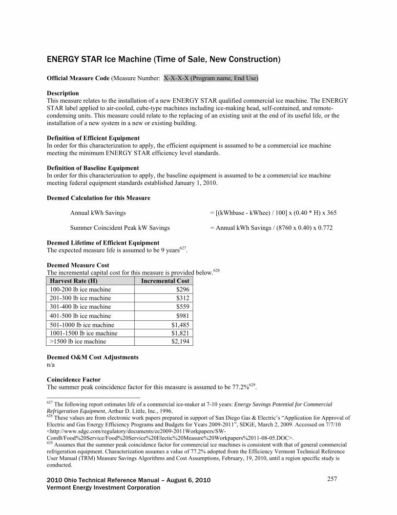
2010 Ohio Technical Reference Manual – August 6, 2010 257 Vermont Energy Investment Corporation
ENERGY STAR Ice Machine (Time of Sale, New Construction) Official Measure Code (Measure Number: X-X-X-X (Program name, End Use) Description This measure relates to the installation of a new ENERGY STAR qualified commercial ice machine. The ENERGY STAR label applied to air-cooled, cube-type machines including ice-making head, self-contained, and remote-condensing units. This measure could relate to the replacing of an existing unit at the end of its useful life, or the installation of a new system in a new or existing building. Definition of Efficient Equipment In order for this characterization to apply, the efficient equipment is assumed to be a commercial ice machine meeting the minimum ENERGY STAR efficiency level standards. Definition of Baseline Equipment In order for this characterization to apply, the baseline equipment is assumed to be a commercial ice machine meeting federal equipment standards established January 1, 2010. Deemed Calculation for this Measure
Annual kWh Savings = [(kWhbase - kWhee) / 100] x (0.40 * H) x 365
Summer Coincident Peak kW Savings = Annual kWh Savings / (8760 x 0.40) x 0.772
Deemed Lifetime of Efficient Equipment The expected measure life is assumed to be 9 years627. Deemed Measure Cost The incremental capital cost for this measure is provided below.628 Harvest Rate (H) Incremental Cost 100-200 lb ice machine $296 201-300 lb ice machine $312 301-400 lb ice machine $559
401-500 lb ice machine $981
501-1000 lb ice machine $1,485 1001-1500 lb ice machine $1,821 >1500 lb ice machine $2,194
Deemed O&M Cost Adjustments n/a Coincidence Factor The summer peak coincidence factor for this measure is assumed to be 77.2%629.
627 The following report estimates life of a commercial ice-maker at 7-10 years: Energy Savings Potential for Commercial Refrigeration Equipment, Arthur D. Little, Inc., 1996. 628 These values are from electronic work papers prepared in support of San Diego Gas & Electric’s “Application for Approval of Electric and Gas Energy Efficiency Programs and Budgets for Years 2009-2011”, SDGE, March 2, 2009. Accessed on 7/7/10 <http://www.sdge.com/regulatory/documents/ee2009-2011Workpapers/SW-ComB/Food%20Service/Food%20Service%20Electic%20Measure%20Workpapers%2011-08-05.DOC>. 629 Assumes that the summer peak coincidence factor for commercial ice machines is consistent with that of general commercial refrigeration equipment. Characterization assumes a value of 77.2% adopted from the Efficiency Vermont Technical Reference User Manual (TRM) Measure Savings Algorithms and Cost Assumptions, February, 19, 2010, until a region specific study is conducted.
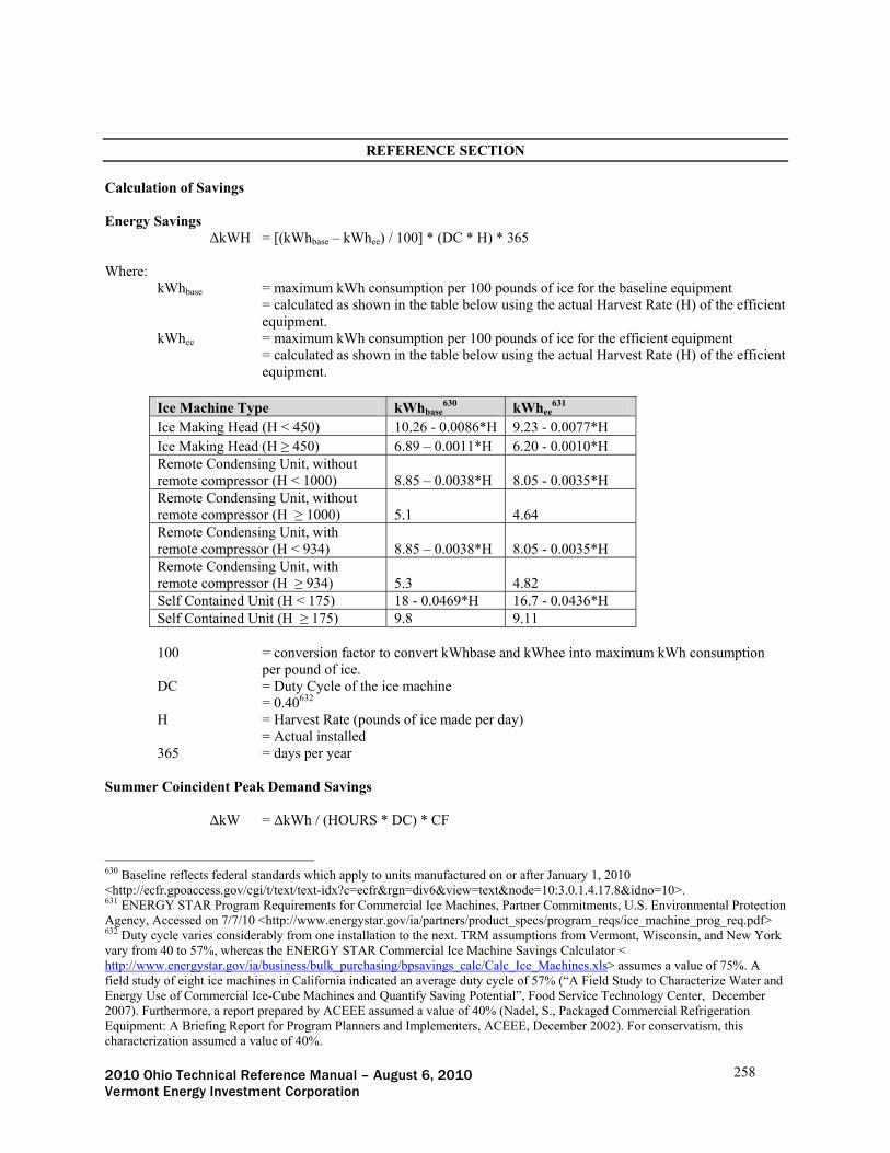
2010 Ohio Technical Reference Manual – August 6, 2010 258 Vermont Energy Investment Corporation
REFERENCE SECTION
Calculation of Savings Energy Savings
ΔkWH = [(kWhbase – kWhee) / 100] * (DC * H) * 365
Where: kWhbase = maximum kWh consumption per 100 pounds of ice for the baseline equipment = calculated as shown in the table below using the actual Harvest Rate (H) of the efficient
equipment. kWhee = maximum kWh consumption per 100 pounds of ice for the efficient equipment
= calculated as shown in the table below using the actual Harvest Rate (H) of the efficient equipment.
Ice Machine Type kWhbase630 kWhee
631 Ice Making Head (H < 450) 10.26 - 0.0086*H 9.23 - 0.0077*H Ice Making Head (H ≥ 450) 6.89 – 0.0011*H 6.20 - 0.0010*H Remote Condensing Unit, without remote compressor (H < 1000) 8.85 – 0.0038*H 8.05 - 0.0035*H Remote Condensing Unit, without remote compressor (H ≥ 1000) 5.1 4.64 Remote Condensing Unit, with remote compressor (H < 934) 8.85 – 0.0038*H 8.05 - 0.0035*H Remote Condensing Unit, with remote compressor (H ≥ 934) 5.3 4.82 Self Contained Unit (H < 175) 18 - 0.0469*H 16.7 - 0.0436*H Self Contained Unit (H ≥ 175) 9.8 9.11
100 = conversion factor to convert kWhbase and kWhee into maximum kWh consumption
per pound of ice. DC = Duty Cycle of the ice machine = 0.40632 H = Harvest Rate (pounds of ice made per day) = Actual installed 365 = days per year
Summer Coincident Peak Demand Savings
ΔkW = ΔkWh / (HOURS * DC) * CF
630 Baseline reflects federal standards which apply to units manufactured on or after January 1, 2010 <http://ecfr.gpoaccess.gov/cgi/t/text/text-idx?c=ecfr&rgn=div6&view=text&node=10:3.0.1.4.17.8&idno=10>. 631 ENERGY STAR Program Requirements for Commercial Ice Machines, Partner Commitments, U.S. Environmental Protection Agency, Accessed on 7/7/10 <http://www.energystar.gov/ia/partners/product_specs/program_reqs/ice_machine_prog_req.pdf> 632 Duty cycle varies considerably from one installation to the next. TRM assumptions from Vermont, Wisconsin, and New York vary from 40 to 57%, whereas the ENERGY STAR Commercial Ice Machine Savings Calculator < http://www.energystar.gov/ia/business/bulk_purchasing/bpsavings_calc/Calc_Ice_Machines.xls> assumes a value of 75%. A field study of eight ice machines in California indicated an average duty cycle of 57% (“A Field Study to Characterize Water and Energy Use of Commercial Ice-Cube Machines and Quantify Saving Potential”, Food Service Technology Center, December 2007). Furthermore, a report prepared by ACEEE assumed a value of 40% (Nadel, S., Packaged Commercial Refrigeration Equipment: A Briefing Report for Program Planners and Implementers, ACEEE, December 2002). For conservatism, this characterization assumed a value of 40%.

2010 Ohio Technical Reference Manual – August 6, 2010 259 Vermont Energy Investment Corporation
Where:
HOURS = annual operating hours = 8760633 CF = Summer Peak Coincidence Factor for measure
= 0.772 634
Fossil Fuel Impact Descriptions and Calculation n/a Water Impact Descriptions and Calculation While the ENERGY STAR labeling criteria require that certified commercial ice machines meet certain “maximum potable water use per 100 pounds of ice made” requirements, such requirements are intended to prevent equipment manufacturers from gaining energy efficiency at the cost of water consumptions. A review of the AHRI Certification Directory635 indicates that approximately 81% of air-cooled, cube-type machines meet the ENERGY STAR potable water use requirement. Therefore, there are no assumed water impacts for this measure. Deemed O&M Cost Adjustment Calculation n/a Version Date & Revision History Draft: Portfolio # Effective date: Date TRM will become effective End date: Date TRM will cease to be effective (or TBD)
633 Unit is assumed to be connected to power 24 hours per day, 365 days per year. 634 Assumes that the summer peak coincidence factor for commercial ice machines is consistent with that of general commercial refrigeration equipment. Characterization assumes a value of 77.2% adopted from the Efficiency Vermont Technical Reference User Manual (TRM) Measure Savings Algorithms and Cost Assumptions, February, 19, 2010, until a region specific study is conducted. 635 AHRI Certification Directory, Accessed on 7/7/10. <http://www.ahridirectory.org/ahridirectory/pages/home.aspx>

2010 Ohio Technical Reference Manual – August 6, 2010 260 Vermont Energy Investment Corporation
Commercial Solid Door Refrigerators & Freezers (Time of Sale, New Construction) Official Measure Code (Measure Number: X-X-X-X (Program name, End Use) Description This measure relates to the installation of a new reach-in commercial refrigerator or freezer meeting ENERGY STAR efficiency standards. ENERGY STAR labeled commercial refrigerators and freezers are more energy efficient because they are designed with components such as ECM evaporator and condenser fan motors, hot gas anti-sweat heaters, or high-efficiency compressors, which will significantly reduce energy consumption. This measure could relate to the replacing of an existing unit at the end of its useful life, or the installation of a new system in a new or existing building. Definition of Efficient Equipment In order for this characterization to apply, the efficient equipment is assumed to be a solid or glass door refrigerator or freezer meeting the minimum ENERGY STAR efficiency level standards. Definition of Baseline Equipment In order for this characterization to apply, the baseline equipment is assumed to be a solid or glass door refrigerator or freezer meeting the minimum federal manufacturing standards as specified by the Energy Policy Act of 2005. Deemed Calculation for this Measure
Annual kWh Savings = (kWhbase – kWhee) * 365
Summer Coincident Peak kW Savings = Annual kWh Savings / HOURS * CF
Deemed Lifetime of Efficient Equipment The expected measure life is assumed to be 12 years 636. Deemed Measure Cost The incremental capital cost for this measure is provided below637.
Type Refrigerator Incremental Cost
Freezer Incremental Cost
Solid or Glass Door 0 < V < 15 $143 $142 15 ≤ V < 30 $164 $166 30 ≤ V < 50 $164 $166 V ≥ 50 $249 $407
636 2008 Database for Energy-Efficiency Resources (DEER), Version 2008.2.05, “Effective/Remaining Useful Life Values”, California Public Utilities Commission, December 16, 2008. http://www.ctsavesenergy.org/files/Measure%20Life%20Report%202007.pdf 637 Estimates of the incremental cost of commercial refrigerators and freezers varies widely by source. Nadel, S., Packaged Commercial Refrigeration Equipment: A Briefing Report for Program Planners and Implementers, ACEEE, December 2002, indicates that incremental cost is approximately zero. Efficiency Vermont Technical Reference User Manual (TRM) Measure Savings Algorithms and Cost Assumptions, February, 19, 2010, assumed incremental cost ranging from $75 to $125 depending on equipment volume. ACEEE notes that incremental cost ranges from 0 to 10% of the baseline unit cost <http://www.aceee.org/ogeece/ch5_reach.htm>. For the purposes of this characterization, assume and incremental cost adder of 5% on the full unit costs presented in Goldberg et al, State of Wisconsin Public Service Commission of Wisconsin, Focus on Energy Evaluation, Business Programs: Incremental Cost Study, KEMA, October 28, 2009.

2010 Ohio Technical Reference Manual – August 6, 2010 261 Vermont Energy Investment Corporation
Deemed O&M Cost Adjustments n/a Coincidence Factor The summer peak coincidence factor for this measure is assumed to be 100%638.
REFERENCE SECTION
Calculation of Savings Energy Savings
ΔkWh = (kWhbase – kWhee) * 365
Where:
kWhbase = baseline maximum daily energy consumption in kWh = calculated using actual chilled or frozen compartment volume (V) of the efficient unit
as shown in the table below.
Type kWhbase639 Solid Door Refrigerator 0.10 * V + 2.04 Glass Door Refrigerator 0.12 * V + 3.34 Solid Door Freezer 0.40 * V + 1.38 Glass Door Freezer 0.75 * V + 4.10
kWhee640 = efficient maximum daily energy consumption in kWh = calculated using actual chilled or frozen compartment volume (V) of the efficient unit
as shown in the table below.
Type Refrigerator kWhee
Freezer kWhee
Solid Door 0 < V < 15 ≤ 0.089V + 1.411 ≤ 0.250V + 1.250 15 ≤ V < 30 ≤ 0.037V + 2.200 ≤ 0.400V – 1.000 30 ≤ V < 50 ≤ 0.056V + 1.635 ≤ 0.163V + 6.125 V ≥ 50 ≤ 0.060V + 1.416 ≤ 0.158V + 6.333 Glass Door 0 < V < 15 ≤ 0.118V + 1.382 ≤ 0.607V + 0.893 15 ≤ V < 30 ≤ 0.140V + 1.050 ≤ 0.733V – 1.000 30 ≤ V < 50 ≤ 0.088V + 2.625 ≤ 0.250V + 13.500 V ≥ 50 ≤ 0.110V + 1.500 ≤ 0.450V + 3.500
V = the chilled or frozen compartment volume (ft3) (as defined in the Association of Home
Appliance Manufacturers Standard HRF1–1979) = Actual installed 365 = days per year
638 The Summer Peak Coincidence Factor is assumed to equal 1.0, since the annual kWh savings is divided by the total annual hours (8760), effectively resulting in the average kW reduction during the peak period. 639 Energy Policy Act of 2005. Accessed on 7/7/10. <http://www.epa.gov/oust/fedlaws/publ_109-058.pdf> 640 ENERGY STAR Program Requirements for Commercial Refrigerators and Freezers Partner Commitments Version 2.0, U.S. Environmental Protection Agency, Accessed on 7/7/10. < http://www.energystar.gov/ia/partners/product_specs/program_reqs/commer_refrig_glass_prog_req.pdf>

2010 Ohio Technical Reference Manual – August 6, 2010 262 Vermont Energy Investment Corporation
Summer Coincident Peak Demand Savings
ΔkW = ΔkW / HOURS * CF
Where:
HOURS = equipment is assumed to operate continuously, 24 hours per day, 365 days per year. = 8760 CF = Summer Peak Coincidence Factor for measure
= 1.0 641 Fossil Fuel Impact Descriptions and Calculation n/a Water Impact Descriptions and Calculation n/a Deemed O&M Cost Adjustment Calculation n/a Version Date & Revision History Draft: Portfolio # Effective date: Date TRM will become effective End date: Date TRM will cease to be effective (or TBD)
641 The Summer Peak Coincidence Factor is assumed to equal 1.0, since the annual kWh savings is divided by the total annual hours (8760), effectively resulting in the average kW reduction during the peak period.

2010 Ohio Technical Reference Manual – August 6, 2010 263 Vermont Energy Investment Corporation
Strip Curtain for Walk-in Coolers and Freezers (New Construction, Retrofit – New Equipment, Retrofit – Early Replacement) Official Measure Code (Measure Number: X-X-X-X (Program name, End Use) Description This commercial measure pertains to the installation of infiltration barriers (strip curtains) on walk-in coolers or freezers. Strip curtains impede heat transfer from adjacent warm and humid spaces into walk-ins when the main door is opened, thereby reducing the cooling load. As a result, compressor run time and energy consumption are reduced. The engineering assumption is that walk-in door is open 2.5 hours per day every day, and the strip curtain covers the entire door frame. Eligible applications include new construction and retrofit. Definition of Efficient Equipment The efficient equipment is a polyethylene strip curtain added to a walk-in cooler or freezer. Definition of Baseline Equipment The baseline assumption is a walk-in cooler or freezer that previously had either no strip curtain installed or an old, ineffective strip curtain installed. Deemed Savings for this Measure
Annual kWh Savings642 = 2,974 for freezers = 422 for coolers
Summer Coincident Peak kW Savings = 0.34 for freezers = 0.05 for coolers
Deemed Lifetime of Efficient Equipment The expected measure life is assumed to be 6 years643. Deemed Measure Cost The incremental capital cost for this measure is $10.22 per square foot of door opening (includes material and labor)
644. Deemed O&M Cost Adjustments n/a Coincidence Factor The summer peak coincidence factor for this measure is 100%645.
642 Values based on analysis prepared by ADM for FirstEnergy utilities in Pennsylvania, provided via personal communication with Diane Rapp of FirstEnergy on June 4, 2010. Based on a review of deemed savings assumptions and methodologies from Oregon and California, the values from Pennsylvania appear reasonable and are the most applicable to the Ohio climate. 643 M. Goldberg, J. Ryan Barry, B. Dunn, M. Ackley, J. Robinson, and D. Deangelo-Woolsey, KEMA. “Focus on Energy: Business Programs – Measure Life Study”, August 2009. 644 2008 Database for Energy-Efficiency Resources (DEER), Version 2008.2.05, “Cost Values and Summary Documentation”, California Public Utilities Commission, December 16, 2008 645 The summer coincident peak demand reduction is assumed as the total annual savings divided by the total number of hours per year, effectively assuming the average demand reduction is realized during the peak period. This is a reasonable assumption for refrigeration savings.

2010 Ohio Technical Reference Manual – August 6, 2010 264 Vermont Energy Investment Corporation
REFERENCE SECTION
Calculation of Savings Energy Savings
ΔkWh = 2,974 for freezers = 422 for coolers
Summer Coincident Peak Demand Savings
ΔkW = ΔkWh / 8760 * CF = 0.35 for freezers = 0.05 for coolers
Where: 8760 = hours per year CF = Summer Peak Coincidence Factor for the measure = 1.0 Fossil Fuel Impact Descriptions and Calculation n/a Water Impact Descriptions and Calculation n/a Deemed O&M Cost Adjustment Calculation n/a Version Date & Revision History Draft: Portfolio # Effective date: Date TRM will become effective End date: Date TRM will cease to be effective (or TBD)

2010 Ohio Technical Reference Manual – August 6, 2010 265 Vermont Energy Investment Corporation
Motors (Time of Sale) Official Measure Code (Measure Number: X-X-X-X (Program name, End Use) Description Three phase Open Drip Proof (ODP) and Totally Enclosed Fan-Cooled (TEFC) motors of at least 1 horsepower (HP) and less than or equal to 200 HP. Definition of Efficient Equipment The efficient equipment is motors meeting the minimum efficiency levels of NEMA premium efficiency motors. Definition of Baseline Equipment For 2010, the baseline equipment assumes motors that meet the minimum efficiency allowed under the Federal Energy Policy Act of 1992 (EPACT). While EPACT generally reflects the floor of efficiencies available, most manufacturers produce models just meeting EPACT, and these are the most commonly purchased among customers not choosing high efficiency. Refer to the table of Baseline Motor Efficiencies in the reference table section. For 2011, NEMA premium efficiency motors are becoming the new baseline. The Energy Independence and Security Act of 2007 (EISA) requires that general purpose motors (subtype I) manufactured after Dec. 19, 2010, from 1 to 200 HP, inclusive, shall have a nominal full-load efficiency that is not less than as defined in NEMA MG 1-2006 Table 12-12 ("NEMA Premium" efficiency levels)646, Therefore, , it is not anticipated that time-of-sale NEMA premium efficient motors will provide savings in 2011. Deemed Savings for this Measure
Annual kWh Savings = 0.746 x [(hpbase X RLFbase)/ηbase – (hpee X RLFee)/ηee]
Summer Coincident Peak kW Savings = ΔkW x CF
Deemed Lifetime of Efficient Equipment 16 years647 Deemed Measure Cost See ‘Incremental Costs for Efficient Motors’ in the Reference Table section below Deemed O&M Cost Adjustments n/a Coincidence Factor 0.38
REFERENCE SECTION
Calculation of Savings Energy Savings
ΔkWh = ΔkW x EFLH
646 NEMA Premium Efficiency Levels Adopted as Federal Motor Efficiency Performance Standards, NEMA press release , March 27, 2008, http://www.nema.org/media/pr/20080327a.cfm, accessed on August 5, 2010. 647 PA Consulting Group, Inc. (2009). Business Programs: Measure Life Study. Prepared for State of Wisconsin Public Service Commission

2010 Ohio Technical Reference Manual – August 6, 2010 266 Vermont Energy Investment Corporation
Where: EFLH = Equivalent Full Load Hours
= site specific variable, either collected on a per unit basis, or calculated using building type and location
Summer Coincident Peak Demand Savings
ΔkW = 0.746 x [(hpbase X RLFbase)/ηbase – (hpee X RLFee)/ηee] kW = ΔkW x CF Where:
hpee = Rated horsepower of the efficient motor
= Nameplate hpbase = Rated horsepower of baseline motor
= same as the efficient motor RLFbase = Rated load factor of baseline motor
= 0.75648 RLFee = Rated load factor of efficient motor = Nameplate ηbase = Efficiency of baseline motor = see ‘Baseline Motor Efficiencies (EPACT)’ below
ηeff = Efficiency of efficient motor = nameplate, must meet or exceed efficiency levels in table ‘Efficient Motor Efficiencies (NEMA Premium)’ found below
0.746 = the conversion factor kW/hp CF = Peak coincidence factor = 0.38649
Fossil Fuel Impact Descriptions and Calculation n/a Water Impact Descriptions and Calculation n/a Deemed O&M Cost Adjustment Calculation n/a Reference Tables Baseline Motor Efficiencies (EPACT)
Open Drip Proof (ODP) # of Poles
Totally Enclosed Fan-Cooled (TEFC)
6 4 2 6 4 2 Speed (RPM) Speed (RPM)
Size HP
1200 1800 3600 1200 1800 3600 1 80.0% 82.5% 75.5% 80.0% 82.5% 75.5%
1.5 84.0% 84.0% 82.5% 85.5% 84.0% 82.5% 2 85.5% 84.0% 84.0% 86.5% 84.0% 84.0% 3 86.5% 86.5% 84.0% 87.5% 87.5% 85.5% 5 87.5% 87.5% 85.5% 87.5% 87.5% 87.5%
7.5 88.5% 88.5% 87.5% 89.5% 89.5% 88.5% 10 90.2% 89.5% 88.5% 89.5% 89.5% 89.5%
648 Efficiency Vermont Technical Reference User Manual (TRM) Measure Savings Algorithms and Cost Assumptions, February, 19, 2010 649 JCP&L metered data

2010 Ohio Technical Reference Manual – August 6, 2010 267 Vermont Energy Investment Corporation
Open Drip Proof (ODP) # of Poles
Totally Enclosed Fan-Cooled (TEFC)
6 4 2 6 4 2 Speed (RPM) Speed (RPM)
Size HP
1200 1800 3600 1200 1800 3600 15 90.2% 91.0% 89.5% 90.2% 91.0% 90.2% 20 91.0% 91.0% 90.2% 90.2% 91.0% 90.2% 25 91.7% 91.7% 91.0% 91.7% 92.4% 91.0% 30 92.4% 92.4% 91.0% 91.7% 92.4% 91.0% 40 93.0% 93.0% 91.7% 93.0% 93.0% 91.7% 50 93.0% 93.0% 92.4% 93.0% 93.0% 92.4% 60 93.6% 93.6% 93.0% 93.6% 93.6% 93.0% 75 93.6% 94.1% 93.0% 93.6% 94.1% 93.0% 100 94.1% 94.1% 93.0% 94.1% 94.5% 93.6% 125 94.1% 94.5% 93.6% 94.1% 94.5% 94.5% 150 94.5% 95.0% 93.6% 95.0% 95.0% 94.5% 200 94.5% 95.0% 94.5% 95.0% 95.0% 95.0%
Efficient Motor Efficiencies (NEMA Premium)
Open Drip Proof (ODP) Totally Enclosed Fan-
Cooled (TEFC) # of Poles # of Poles
2 4 6 2 4 6 Speed (RPM) Speed (RPM)
Size HP
1200 1800 3600 1200 1800 3600 1 82.50% 85.50% 77.00% 82.50% 85.50% 77.00%
1.5 86.50% 86.50% 84.00% 87.50% 86.50% 84.00% 2 87.50% 86.50% 85.50% 88.50% 86.50% 85.50% 3 88.50% 89.50% 85.50% 89.50% 89.50% 86.50% 5 89.50% 89.50% 86.50% 89.50% 89.50% 88.50%
7.5 90.20% 91.00% 88.50% 91.00% 91.70% 89.50% 10 91.70% 91.70% 89.50% 91.00% 91.70% 90.20% 15 91.70% 93.00% 90.20% 91.70% 92.40% 91.00% 20 92.40% 93.00% 91.00% 91.70% 93.00% 91.00% 25 93.00% 93.60% 91.70% 93.00% 93.60% 91.70% 30 93.60% 94.10% 91.70% 93.00% 93.60% 91.70% 40 94.10% 94.10% 92.40% 94.10% 94.10% 92.40% 50 94.10% 94.50% 93.00% 94.10% 94.50% 93.00% 60 94.50% 95.00% 93.60% 94.50% 95.00% 93.60% 75 94.50% 95.00% 93.60% 94.50% 95.40% 93.60%
100 95.00% 95.40% 93.60% 95.00% 95.40% 94.10% 125 95.00% 95.40% 94.10% 95.00% 95.40% 95.00% 150 95.40% 95.80% 94.10% 95.80% 95.80% 95.00% 200 95.40% 95.80% 95.00% 95.80% 96.20% 95.40%

2010 Ohio Technical Reference Manual – August 6, 2010 268 Vermont Energy Investment Corporation
Incremental Costs for Efficient Motors650
Open Drip-Proof (ODP)
Totally Enclosed Fan-Cooled
(TEFC) Size HP Incremental Cost Incremental Cost
1 $52 $52 1.5 $60 $60
2 $61 $61 3 $54 $54 5 $63 $63
7.5 $123 $123 10 $116 $116 15 $115 $115 20 $115 $115 25 $201 $201 30 $231 $231 40 $249 $249 50 $273 $273 60 $431 $431 75 $554 $554
100 $658 $658 125 $841 $841 150 $908 $908 200 $964 $964
Version Date & Revision History Draft: Portfolio # Effective date: Date TRM will become effective End date: Date TRM will cease to be effective (or TBD)
650 Xenergy (2001). Motor Up! Program Evaluation and Market Assessment

2010 Ohio Technical Reference Manual – August 6, 2010 269 Vermont Energy Investment Corporation
High Efficiency Pumps and Pumping Efficiency Improvements (Retrofit) Official Measure Code (Measure Number: X-X-X-X (Program name, End Use) Description Pump improvements can be done to optimize the design and control of water pumping systems. The measurement of energy and demand savings for commercial and industrial applications will vary with the type of pumping technology, operating hours, efficiency and current and proposed controls. Depending on the specific application, slowing the pump, trimming or replacing the impeller, or replacing the pump may suitable options for improving pumping efficiency. Definition of Efficient Equipment In order for this characterization to apply, the efficient equipment is assumed to be an optimized pumping system meeting applicable program efficiency requirements. Definition of Baseline Equipment In order for this characterization to apply, the baseline equipment is assumed to be a non-optimized existing pumping system. Deemed Calculation for this Measure
Annual kWh Savings651 = (HPmotor * LF * 0.746 / ηmotor) * HOURS * (ESF/ηpump) Summer Coincident Peak kW Savings = (HPmotor * LF * 0.746 / ηmotor) * (ESF/ηpump) * CF
Deemed Lifetime of Efficient Equipment The expected measure life is assumed to be 10 years652. Deemed Measure Cost The incremental capital cost for this measure can vary considerably depending upon the strategy employed to achieve the required efficiency levels and should be determined on a site-specific basis. Deemed O&M Cost Adjustments n/a Coincidence Factor The summer peak coincidence factor for this measure is assumed to be 38%653.
REFERENCE SECTION
Calculation of Savings Energy Savings
ΔkWh = (HPmotor * LF * 0.746 / ηmotor) * HOURS * (ESF/ηpump) Where:
651 Improving Pumping System Performance: A Sourcebook for Industry, Second Edition, U.S. Department of Energy, May 2006 652 Martin, N. et al., Emerging Energy-Efficient Industrial Technologies: New York State Edition, American Council for an Energy Efficient Economy (ACEEE), March 2001 653 Summer Peak Coincidence Factor has been preserved from the “Technical Reference Manual (TRM) for Ohio Senate Bill 221 Energy Efficiency and Conservation Program and 09-512-GE-UNC”, October 15, 2009. This is likely a conservative estimate, but is recommended for further study.

2010 Ohio Technical Reference Manual – August 6, 2010 270 Vermont Energy Investment Corporation
HPmotor = nameplate motor horsepower = Actual installed LF = Load Factor; Ratio of the peak running load to the nameplate rating of the motor. If
unknown, assume a value of 80%654. 0.746 = conversion factor from horse-power to kW (kW/hp) ηmotor = Motor efficiency; if actual motor efficiency at typical pump operating conditions is
unknown, assume the federal minimum efficiency requirements as below:
Open Drip Proof (ODP)# of Poles
Totally Enclosed Fan-Cooled (TEFC)
6 4 2 6 4 2 Speed (RPM) Speed (RPM)
Size HP
1200 1800 3600 1200 1800 3600 1 80.0% 82.5% 75.5% 80.0% 82.5% 75.5%
1.5 84.0% 84.0% 82.5% 85.5% 84.0% 82.5% 2 85.5% 84.0% 84.0% 86.5% 84.0% 84.0% 3 86.5% 86.5% 84.0% 87.5% 87.5% 85.5% 5 87.5% 87.5% 85.5% 87.5% 87.5% 87.5%
7.5 88.5% 88.5% 87.5% 89.5% 89.5% 88.5% 10 90.2% 89.5% 88.5% 89.5% 89.5% 89.5% 15 90.2% 91.0% 89.5% 90.2% 91.0% 90.2% 20 91.0% 91.0% 90.2% 90.2% 91.0% 90.2%
HOURS = annual operating hours of the pump = Actual installed ESF = Energy Savings Factor; assume a value of 15%655. ηpump = Pump efficiency at design point; if actual pump efficiency is unknown, assume program
compliance efficiency as below:
HP Minimum Pump Efficiency at Design Point (ηpump)
1.5 65% 2 65% 3 67% 5 70%
7.5 73% 10 75% 15 77% 20 77%
Summer Coincident Peak Demand Savings
ΔkW = (HPmotor * LF * 0.746 / ηmotor) * (ESF/ηpump) * CF
Where: CF = Summer Peak Coincidence Factor for measure
= 0.38656
654 In many applications, the pump/motor assembly is oversized. For analysis purposes, a typical 80% load factor is assumed; however, this assumption should be verified through evaluation if significant savings are realized through prescriptive pumping efficiency improvements. 655 Published estimates of typical pumping efficiency improvements range from 10 to 20%. For analysis purposes, assume 15%. Martin, N. et al., Emerging Energy-Efficient Industrial Technologies: New York State Edition, American Council for an Energy Efficient Economy (ACEEE), March 2001. 656 Summer Peak Coincidence Factor has been preserved from the “Technical Reference Manual (TRM) for Ohio Senate Bill 221 Energy Efficiency and Conservation Program and 09-512-GE-UNC”, October 15, 2009. This is likely a conservative estimate, but is recommended for further study.

2010 Ohio Technical Reference Manual – August 6, 2010 271 Vermont Energy Investment Corporation
Fossil Fuel Impact Descriptions and Calculation n/a Water Impact Descriptions and Calculation n/a Deemed O&M Cost Adjustment Calculation n/a Version Date & Revision History Draft: Portfolio # Effective date: Date TRM will become effective End date: Date TRM will cease to be effective (or TBD)

2010 Ohio Technical Reference Manual – August 6, 2010 272 Vermont Energy Investment Corporation
Efficient Air Compressors (Time of Sale) Official Measure Code (Measure Number: X-X-X-X (Program name, End Use) Description This measure relates to the installation of an air compressor with a variable frequency drive, load/no load controls, or variable displacement controls. Baseline compressors choke off the inlet air to modulate the compressor output, which is not efficient. Efficient compressors use less energy at part load conditions. Demand curves are as per DOE data for a Variable Speed compressor versus a Modulating compressor. This measure could relate to the replacing of an existing unit at the end of its useful life, or the installation of a new system in a new building (i.e. time of sale). Definition of Efficient Equipment In order for this characterization to apply, the efficient equipment is assumed to be an air compressor with a variable frequency drive, load/no load controls657, or variable displacement controls. Definition of Baseline Equipment In order for this characterization to apply, the baseline equipment is assumed to be a modulating air compressor with blow down. Deemed Calculation for this Measure
Annual kWh Savings = BHP * 0.746 / ηmotor x HOURS x ESF Summer Coincident Peak kW Savings = Annual kWh Savings / HOURS * CF
Deemed Lifetime of Efficient Equipment The expected measure life is assumed to be 15 years 658. Deemed Measure Cost The incremental capital costs for this measure should be determined on a case-by-case basis. For analysis purposes, assume the incremental costs specified below: Compressor Type Incremental Cost659
Load/No Load $200/hp Variable Displacement $250/hp Variable Frequency Drive $300/hp Deemed O&M Cost Adjustments n/a Coincidence Factor The summer peak coincidence factor for this measure is assumed to be 38%660.
657 For analysis purposes, it is assumed that the compressed air system with load / no load controls utilizes an air receiver with a storage capacity of 5 gallons per cubic foot per minute of compressor capacity. 658 Based on a review of TRM assumptions from Vermont, New Hampshire, Massachusetts, and Wisconsin. Estimates range from 10 to 15 years. 659 Incremental cost estimates have been maintained from the “Technical Reference Manual (TRM) for Ohio Senate Bill 221 Energy Efficiency and Conservation Program and 09-512-GE-UNC”, October 15, 2009, and appear reasonable. However, future study of these estimates is recommended as published estimates of incremental costs for efficient air compressors are scarce. 660 Summer Peak Coincidence Factor has been preserved from the “Technical Reference Manual (TRM) for Ohio Senate Bill 221 Energy Efficiency and Conservation Program and 09-512-GE-UNC”, October 15, 2009. This is likely a conservative estimate, but is recommended for further study.
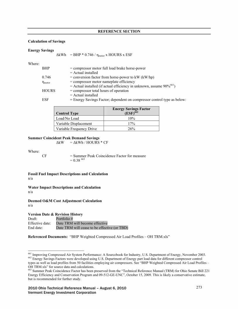
2010 Ohio Technical Reference Manual – August 6, 2010 273 Vermont Energy Investment Corporation
REFERENCE SECTION
Calculation of Savings Energy Savings
ΔkWh = BHP * 0.746 / ηmotor x HOURS x ESF
Where: BHP = compressor motor full load brake horse-power = Actual installed 0.746 = conversion factor from horse-power to kW (kW/hp) ηmotor = compressor motor nameplate efficiency = Actual installed (if actual efficiency in unknown, assume 90%661) HOURS = compressor total hours of operation = Actual installed ESF = Energy Savings Factor; dependent on compressor control type as below:
Control Type Energy Savings Factor
(ESF)662 Load/No Load 10% Variable Displacement 17% Variable Frequency Drive 26%
Summer Coincident Peak Demand Savings
ΔkW = ΔkWh / HOURS * CF
Where: CF = Summer Peak Coincidence Factor for measure
= 0.38 663 Fossil Fuel Impact Descriptions and Calculation n/a Water Impact Descriptions and Calculation n/a Deemed O&M Cost Adjustment Calculation n/a Version Date & Revision History Draft: Portfolio # Effective date: Date TRM will become effective End date: Date TRM will cease to be effective (or TBD) Referenced Documents: “BHP Weighted Compressed Air Load Profiles – OH TRM.xls”
661 Improving Compressed Air System Performance: A Sourcebook for Industry, U.S. Department of Energy, November 2003. 662 Energy Savings Factors were developed using U.S. Department of Energy part load data for different compressor control types as well as load profiles from 50 facilities employing air compressors. See “BHP Weighted Compressed Air Load Profiles – OH TRM.xls” for source data and calculations. 663 Summer Peak Coincidence Factor has been preserved from the “Technical Reference Manual (TRM) for Ohio Senate Bill 221 Energy Efficiency and Conservation Program and 09-512-GE-UNC”, October 15, 2009. This is likely a conservative estimate, but is recommended for further study.

2010 Ohio Technical Reference Manual – August 6, 2010 274 Vermont Energy Investment Corporation
Vending Machine Occupancy Sensors (Time of Sale, New Construction, Retrofit – New Equipment) Official Measure Code (Measure Number: X-X-X-X (Program name, End Use) Description This measure relates to the installation of new controls on refrigerated beverage vending machines, non-refrigerated snack vending machines, and glass front refrigerated coolers. Controls can significantly reduce the energy consumption of vending machine and refrigeration systems. Qualifying controls must power down these systems during periods of inactivity but, in the case of refrigerated machines, must always maintain a cool product that meets customer expectations. This measure relates to the installation of a new control on a new or existing unit. This measure should not be applied to ENERGY STAR qualified vending machines, as they already have built-in controls. Definition of Efficient Equipment In order for this characterization to apply, the efficient equipment is assumed to be a standard efficiency refrigerated beverage vending machine, non-refrigerated snack vending machine, or glass front refrigerated cooler with a control system capable of powering down lighting and refrigeration systems during periods of inactivity. Definition of Baseline Equipment In order for this characterization to apply, the baseline equipment is assumed to be a standard efficiency refrigerated beverage vending machine, non-refrigerated snack vending machine, or glass front refrigerated cooler without a control system capable of powering down lighting and refrigeration systems during periods of inactivity. Deemed Calculation for this Measure
Annual kWh Savings = 8760 x WATTSbase / 1000 x ESF
Summer Coincident Peak kW Savings = 0
Deemed Lifetime of Efficient Equipment The expected measure life is assumed to be 5 years 664. Deemed Measure Cost The actual measure installation cost should be used (including material and labor), but the following can be assumed for analysis purposes665: Refrigerated Vending Machine: $215.50 Non-Refrigerated Vending Machine: $108.00 Deemed O&M Cost Adjustments n/a Coincidence Factor The summer peak coincidence factor for this measure is assumed to be 0666.
664 Measure Life Study, prepared for the Massachusetts Joint Utilities, Energy & Resource Solutions, November 2005. 665 2005 Database for Energy-Efficiency Resources (DEER), Version 2005.21. “Cost Data for Supporting Documents.” 666 Assumed that the peak period is coincident with periods of high traffic diminishing the demand reduction potential of occupancy based controls.

2010 Ohio Technical Reference Manual – August 6, 2010 275 Vermont Energy Investment Corporation
REFERENCE SECTION
Calculation of Savings Energy Savings
ΔkWh = WATTSbase / 1000 * HOURS * ESF
Where: WATTSbase = connected kW of the controlled equipment; see table below for default values by
connected equipment type:
Equipment Type WATTSbase667 Refrigerated Beverage Vending Machines 400 Non-Refrigerated Snack Vending Machines 85 Glass Front Refrigerated Coolers 460
1000 = conversion factor (W/kW) HOURS = operating hours of the connected equipment; assumed that the equipment operates 24
hours per day, 365 days per year = 8760 ESF = Energy Savings Factor; represents the percent reduction in annual kWh consumption of
the equipment controlled; see table below for default values:
Equipment Type Energy Savings Factor (ESF)668
Refrigerated Beverage Vending Machines 46% Non-Refrigerated Snack Vending Machines 46% Glass Front Refrigerated Coolers 30%
Summer Coincident Peak Demand Savings
ΔkW669 = 0
Fossil Fuel Impact Descriptions and Calculation n/a Water Impact Descriptions and Calculation n/a Deemed O&M Cost Adjustment Calculation n/a Version Date & Revision History Draft: Portfolio # Effective date: Date TRM will become effective End date: Date TRM will cease to be effective (or TBD)
667 USA Technologies Energy Management Product Sheets, July 2006; cited September 2009. <http:// http://www.usatech.com/energy_management/energy_productsheets.php> 668 Ibid. 669 Assumed that the peak period is coincident with periods of high traffic diminishing the demand reduction potential of occupancy based controls.

2010 Ohio Technical Reference Manual – August 6, 2010 276 Vermont Energy Investment Corporation
Heat Pump Water Heaters (New Construction, Retrofit) Official Measure Code (Measure Number: X-X-X-X (Program name, End Use) Description This measure relates to the installation of a heat pump water heater (HPWH) in place of a standard electric water heater. HPWHs can be added to existing domestic hot water (DHW) systems to improve the overall efficiency. HPWHs utilize refrigerants (like an air source heat pump) and have much higher coefficients of performance (COP) than standard electric water heaters. HPWHs remove waste heat from surrounding air sources and preheat the DHW supply system. HPWHs come in a variety of sizes and the size of HPWH will depend on the desired temperature output and amount of hot water needed by application. The savings from water heater heat pumps will depend on the design, size (capacity), water heating requirements, building application and climate. This measure could relate to either a retrofit or a new installation. Definition of Efficient Equipment In order for this characterization to apply, the efficient equipment is assumed to be a heat pump water heater with or without an auxiliary water heating system. Definition of Baseline Equipment In order for this characterization to apply, the baseline equipment is assumed to be a standard electric storage tank-type water heater with a thermal efficiency of 98%. This measure does not apply to natural gas-fired water heaters. Deemed Calculation for this Measure
Annual kWh Savings = (GPD * 365 * 8.33 * ΔTs ) / (3413 ) * [(1/Et,base) – (1/COP)]
Summer Peak Coincident kW Savings = (GPH * 8.33 * ΔTs ) / (3413) * [(1/Et,base) – (1/COP)] * CF
Deemed Lifetime of Efficient Equipment The expected measure life is assumed to be 10 years670. Deemed Measure Cost Due to the complexity of heat pump water heater systems, incremental capital costs should be determined on a case-by-case basis. High capacity heat pump water heaters will typically have a supplemental heating source such as an electric resistance heater. For new construction applications, the incremental capital cost for this measure should be calculated as the difference in installed cost of the entire heat pump water heater system including any auxiliary heating systems and a standard electric storage tank water heater of comparable capacity. For retrofit applications, the total installed cost of heat pump water heater should be used. Deemed O&M Cost Adjustments n/a Coincidence Factor The summer peak coincidence factor for this measure is assumed to be 6%671.
670 Estimates of measure life from utilities in the Northeast and the U.S. Department of Energy vary from 10 to 15 years. Assume 10 years as a conservative estimate. http://www.ctsavesenergy.org/files/Measure%20Life%20Report%202007.pdf 671 “Technical Reference Manual (TRM) for Ohio Senate Bill 221 Energy Efficiency and Conservation Program and 09-512-GE-UNC”, October 15, 2009. Based on Ohio utility supply profiles.
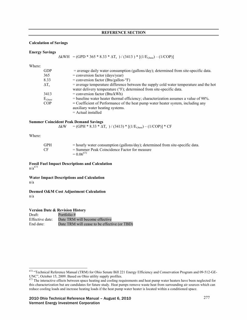
2010 Ohio Technical Reference Manual – August 6, 2010 277 Vermont Energy Investment Corporation
REFERENCE SECTION
Calculation of Savings Energy Savings
ΔkWH = (GPD * 365 * 8.33 * ΔTs ) / (3413 ) * [(1/Et,base) – (1/COP)]
Where: GDP = average daily water consumption (gallons/day); determined from site-specific data. 365 = conversion factor (days/year) 8.33 = conversion factor (Btu/gallon-°F) ΔTs = average temperature difference between the supply cold water temperature and the hot
water delivery temperature (°F); determined from site-specific data. 3413 = conversion factor (Btu/kWh) Et,base = baseline water heater thermal efficiency; characterization assumes a value of 98%. COP = Coefficient of Performance of the heat pump water heater system, including any
auxiliary water heating systems. = Actual installed
Summer Coincident Peak Demand Savings
ΔkW = (GPH * 8.33 * ΔTs ) / (3413) * [(1/Et,base) – (1/COP)] * CF
Where:
GPH = hourly water consumption (gallons/day); determined from site-specific data. CF = Summer Peak Coincidence Factor for measure
= 0.06672 Fossil Fuel Impact Descriptions and Calculation n/a673 Water Impact Descriptions and Calculation n/a Deemed O&M Cost Adjustment Calculation n/a Version Date & Revision History Draft: Portfolio # Effective date: Date TRM will become effective End date: Date TRM will cease to be effective (or TBD)
672 “Technical Reference Manual (TRM) for Ohio Senate Bill 221 Energy Efficiency and Conservation Program and 09-512-GE-UNC”, October 15, 2009. Based on Ohio utility supply profiles. 673 The interactive effects between space heating and cooling requirements and heat pump water heaters have been neglected for this characterization but are candidates for future study. Heat pumps remove waste heat from surrounding air sources which can reduce cooling loads and increase heating loads if the heat pump water heater is located within a conditioned space.

2010 Ohio Technical Reference Manual – August 6, 2010 278 Vermont Energy Investment Corporation
Commercial Clothes Washer (Time of Sale) Official Measure Code (Measure Number: X-X-X-X (Program name, End Use) Description High-efficiency commercial washers are intended for purchase and installation in laundromats, multi-family buildings and institutions. These high-efficiency washers are nearly identical to residential models available in retail outlets, with minor engineering changes, such as the addition of a coin box. High-efficiency commercial washers typically save up to 50 percent of energy costs and use about 30 percent less water. Definition of Efficient Equipment The efficient equipment is defined as a commercial-grade clothes washer meeting the minimum efficiency standards for ENERGY STAR (MEF ≥1.8)674. Also, for this characterization to apply the facility where the equipment is installed must have an electric water heater. Definition of Baseline Equipment The baseline equipment for this measure is a commercial grade clothes washer that meets federal manufacturing standards (MEF ≥ 1.26). Deemed Calculations for this Measure
Annual kWh Savings = ΔkWhLoad x 950
Summer Coincident Peak kW Savings = n/a
Deemed Lifetime of Efficient Equipment The effective measure life for commercial-grade clothes washers is 10 years675 Deemed Measure Cost $347 per unit ENERGY STAR/CEE Tier1, $475 per unit CEE Tier 2, $604 per unit CEE Tier 3676 Deemed O&M Cost Adjustments n/a Coincidence Factor n/a
REFERENCE SECTION
Calculation of Savings Energy Savings
ΔkWh = ΔkWhLoad x LoadsYear
Where: ΔkWhLoad = The difference in electricity consumption per load of laundry between baseline
equipment and efficient equipment = Dependent on energy source for washer677:
674 Beginning in 2011 the criteria will be raised to MEF > 2.0 675 2008 Database for Energy-Efficiency Resources (DEER), Version 2008.2.05, “Effective/Remaining Useful Life Values”, 676 2008 Database for Energy-Efficiency Resources (DEER), Version 2008.2.05, “Cost Values and Summary Documentation”,

2010 Ohio Technical Reference Manual – August 6, 2010 279 Vermont Energy Investment Corporation
Fuel Source ΔkWh per Load Therms per Load Electric Hot Water, Electric Dryer 0.57 0 Gas Hot Water, Electric Dryer 0.25 0.02
LoadYear = Number of loads per year
= 950678
For example, a commercial clothes washer is installed in a facility with electric water heating and electric drying:
ΔkWh = 0.57 x 950
= 541.5 kWh Summer Coincident Peak Demand Savings No demand savings are claimed for this measure since there is insufficient peak coincident data. Fossil Fuel Impact Descriptions and Calculation Commercial clothes washers will only have fossil fuel impacts when either the washer, dryer, or both are powered by gas instead of electricity.
ΔMMBtu = ΔMMBtuLoad x LoadsYear Where:
ΔMMBtuLoad = The difference in gas consumption per load of laundry between baseline equipment and efficient equipment = Dependent on energy source for washer and dryer – see Table ‘Assumptions for Electricity and Gas Consumption for Commercial Clothes Washers’ in the Reference Table Section
LoadsYear = Number of loads per year = 950 Water Impact Descriptions and Calculation The annual water savings for a commercial clothes washer is assumed to be 15,854 gallons per year.679 Deemed O&M Cost Adjustment Calculation n/a Version Date & Revision History Draft: Portfolio # Effective date: Date TRM will become effective End date: Date TRM will cease to be effective (or TBD)
677 ENERGY STAR calculator for Commercial Clothes Washers, values based on the difference between the average of all qualified models and the average of all unqualified models (July 2009). 678 ENERGY STAR calculator for Commercial Clothes Washers, Multi-Family Laundry Association (2002) 679 ENERGY STAR calculator for Commercial Clothes Washers, average water consumption based on all qualified models (July 2009)

2010 Ohio Technical Reference Manual – August 6, 2010 280 Vermont Energy Investment Corporation
Commercial Plug Load – Smart Strip Plug Outlets (Time of Use, Retrofit – New Equipment) Official Measure Code (Measure Number: X-X-X-X (Program name, End Use) Description A smart strip plug outlet is a multi-plug power strip with the ability to automatically disconnect specific loads that are plugged into it depending upon the power draw of a control load, also plugged into the strip. The energy savings are measured by estimating the number of hours that electronic devices at typical workstations are either in the “sleep” mode or shut off and the standby loads consumed by the devices at those times. The smart strip will eliminate these standby loads and result in measureable energy savings. A smart strip plug outlet is purchased through a retail outlet and installed in an office environment where standby loads are uncontrolled. Definition of Efficient Equipment The efficient condition assumes peripherals electronic office equipment is plugged into the controlled Smart Strip outlets resulting in a reduction in standby load. No savings are associated with the control load, or loads plugged into the uncontrolled outlets. Definition of Baseline Equipment The baseline assumes a mix of typical office equipment (computer and peripherals) each with uncontrolled standby load. Deemed Savings for this Measure
Annual kWh Savings = 23.6 kWh
Summer Coincident Peak kW Savings = 0
Deemed Lifetime of Efficient Equipment The estimated useful life for a smart strip plug outlet is 8 years680 Deemed Measure Cost The estimated incremental cost for smart strip plug outlets is assumed to be $15.681 Deemed O&M Cost Adjustments n/a Coincidence Factor 0682
REFERENCE SECTION
Calculation of Savings Energy Savings
ΔkWh = (WORKDAYS x ∆WhWorkday + (365 – WORKDAYS) * ∆WhNon-Workday)/ 1000
680 BC Hydro report: Smart Strip electrical savings and usability, October 2008 (unit can only take one surge, then needs to be replaced) 681 Research Into Action, Inc. (2010) Electronics and Energy Efficiency: A Plug Load Characterization Study. Prepared for Southern California Edison.. Incremental cost over standard power strip with surge protection with average market price of $35 for controlled power strip and $20 for baseline plug strip with surge protection 682 Based on the assumption that most office equipment will be operating during the peak coincident hour
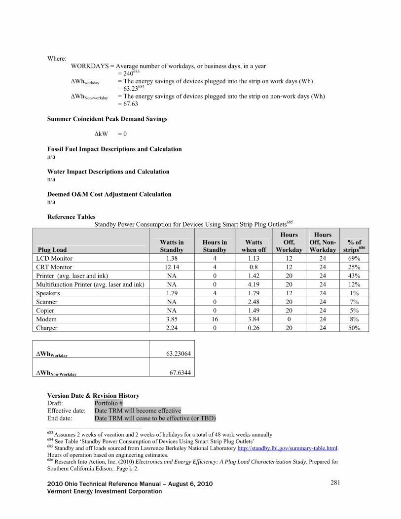
2010 Ohio Technical Reference Manual – August 6, 2010 281 Vermont Energy Investment Corporation
Where:
WORKDAYS = Average number of workdays, or business days, in a year = 240683 ∆Whworkday = The energy savings of devices plugged into the strip on work days (Wh)
= 63.23684 ∆WhNon-workday = The energy savings of devices plugged into the strip on non-work days (Wh)
= 67.63
Summer Coincident Peak Demand Savings ΔkW = 0
Fossil Fuel Impact Descriptions and Calculation n/a Water Impact Descriptions and Calculation n/a Deemed O&M Cost Adjustment Calculation n/a Reference Tables Standby Power Consumption for Devices Using Smart Strip Plug Outlets685
Plug Load Watts in Standby
Hours in Standby
Watts when off
Hours Off,
Workday
Hours Off, Non-Workday
% of strips686
LCD Monitor 1.38 4 1.13 12 24 69% CRT Monitor 12.14 4 0.8 12 24 25% Printer (avg. laser and ink) NA 0 1.42 20 24 43% Multifunction Printer (avg. laser and ink) NA 0 4.19 20 24 12% Speakers 1.79 4 1.79 12 24 1% Scanner NA 0 2.48 20 24 7% Copier NA 0 1.49 20 24 5% Modem 3.85 16 3.84 0 24 8% Charger 2.24 0 0.26 20 24 50%
∆WhWorkday 63.23064
∆WhNon-Workday 67.6344 Version Date & Revision History Draft: Portfolio # Effective date: Date TRM will become effective End date: Date TRM will cease to be effective (or TBD)
683 Assumes 2 weeks of vacation and 2 weeks of holidays for a total of 48 work weeks annually 684 See Table ‘Standby Power Consumption of Devices Using Smart Strip Plug Outlets’ 685 Standby and off loads sourced from Lawrence Berkeley National Laboratory http://standby.lbl.gov/summary-table.html. Hours of operation based on engineering estimates. 686 Research Into Action, Inc. (2010) Electronics and Energy Efficiency: A Plug Load Characterization Study. Prepared for Southern California Edison.. Page k-2.

2010 Ohio Technical Reference Manual – August 6, 2010 282 Vermont Energy Investment Corporation
Plug Load Occupancy Sensor (Retrofit) Official Measure Code (Measure Number: X-X-X-X (Program name, End Use) Description Plug load occupancy sensors are devices that control low wattage office equipment using an occupancy sensor. They typically use an infrared sensor to monitor movement, and use a smart strip to turn off connected devices, or put them in standby mode, when no one is present. Definition of Efficient Equipment In order for this characterization to apply, the installed equipment must be a ‘smart’ power strip with both control and peripheral outlets, and an occupancy sensor. Definition of Baseline Equipment The baseline assumes a mix of typical document station office equipment (printers, scanners, fax machines, etc.) each with uncontrolled standby load. Deemed Savings for this Measure
Annual kWh Savings = 169 kWh/yr Summer Coincident Peak kW Savings = 0
Deemed Lifetime of Efficient Equipment The estimated useful life for a smart strip plug outlet is 8 years687 Deemed Measure Cost The incremental cost for this measure is assumed to be $70688 Deemed O&M Cost Adjustments n/a Coincidence Factor 0689
REFERENCE SECTION
Calculation of Savings Energy Savings
ΔkWh = (WORKDAYS x ∆Wsleep)/ 1000
Where: WORKDAYS = Average number of workdays, or business days, in a year = 240690 ∆Wsleep = The energy savings of devices plugged into the strip when in ‘sleep’ mode (Wh)
= 704691
687 BC Hydro report: Smart Strip electrical savings and usability, October 2008 (unit can only take one surge, then needs to be replaced) 688 Plug Load Characterization Study for Southern California Edison. Prepared by Research Into Action (2010) 689 Based on assumption that office equipment will be running during the peak period 690 Assumes 2 weeks of vacation and 2 weeks of holidays for a total of 48 work weeks annually 691 See Table ‘Standby Power Consumption of Devices Using Smart Strip Plug Outlets’
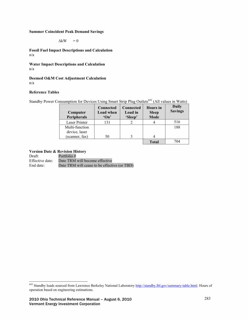
2010 Ohio Technical Reference Manual – August 6, 2010 283 Vermont Energy Investment Corporation
Summer Coincident Peak Demand Savings ΔkW = 0
Fossil Fuel Impact Descriptions and Calculation n/a Water Impact Descriptions and Calculation n/a Deemed O&M Cost Adjustment Calculation n/a Reference Tables Standby Power Consumption for Devices Using Smart Strip Plug Outlets692 (All values in Watts)
Computer Peripherals
Connected Load when
‘On’
Connected Load in ‘Sleep’
Hours in Sleep Mode
Daily Savings
Laser Printer 131 2 4 516 Multi-function device, laser
(scanner, fax) 50 3 4
188
Total 704 Version Date & Revision History Draft: Portfolio # Effective date: Date TRM will become effective End date: Date TRM will cease to be effective (or TBD)
692 Standby loads sourced from Lawrence Berkeley National Laboratory http://standby.lbl.gov/summary-table.html. Hours of operation based on engineering estimations.

2010 Ohio Technical Reference Manual – August 6, 2010 284 Vermont Energy Investment Corporation
Energy Efficient Furnace (Time of Sale, Retrofit – Early Replacement) Official Measure Code (Measure Number: X-X-X-X (Efficient Products, HVAC End Use) Description This measure covers the installation of a high efficiency gas furnace in lieu of a standard efficiency gas furnace. High efficiency gas furnaces achieve savings through the utilization of a sealed, super insulated combustion chamber, more efficient burners, and multiple heat exchangers that remove a significant portion of the waste heat from the flue gasses. Because multiple heat exchangers are used to remove waste heat from the escaping flue gasses, most of the flue gasses condense and must be drained. Furnaces equipped with ECM fan motors can save additional electric energy. Definition of Efficient Equipment The efficient equipment is a natural gas-fired furnace with a minimum Annual Fuel Utilization Efficiency (AFUE) rating of 93%. Definition of Baseline Equipment The equivalent baseline equipment is a natural gas-fired furnace with an AFUE of 80%. Deemed Calculation for this Measure
Annual kWh Savings = 5 x CAP x EFLHh x (ηbase/ηee) Summer Coincident Peak kW Savings = 0693
Annual MMBtu Savings = (CAP) * (EFLHh) * ((1 – (ηbase/ηee)) - MMBtuECM Deemed Lifetime of Efficient Equipment 20694 Deemed Measure Cost Incremental cost estimated at $900695 Deemed O&M Cost Adjustments $0696 Coincidence Factor n/a
REFERENCE SECTION
Calculation of Savings Energy Savings
693 For analysis purposes, it is assumed that the furnace fan does not operate during the summer season and therefore contributes no summer peak coincident savings. 694 Based on engineering modeling by Michael Blasnik (M. Blasnik & Associates) and KEMA in support of “Application of Columbia Gas of Ohio, Inc, to Establish Demand Side Management Programs for Residential and Commercial Consumers,” Filed with the Ohio Public Utilities Commission, Case No. 08-0833-GA-UNC, July 1, 2008 695 Ibid. 696 Ibid.
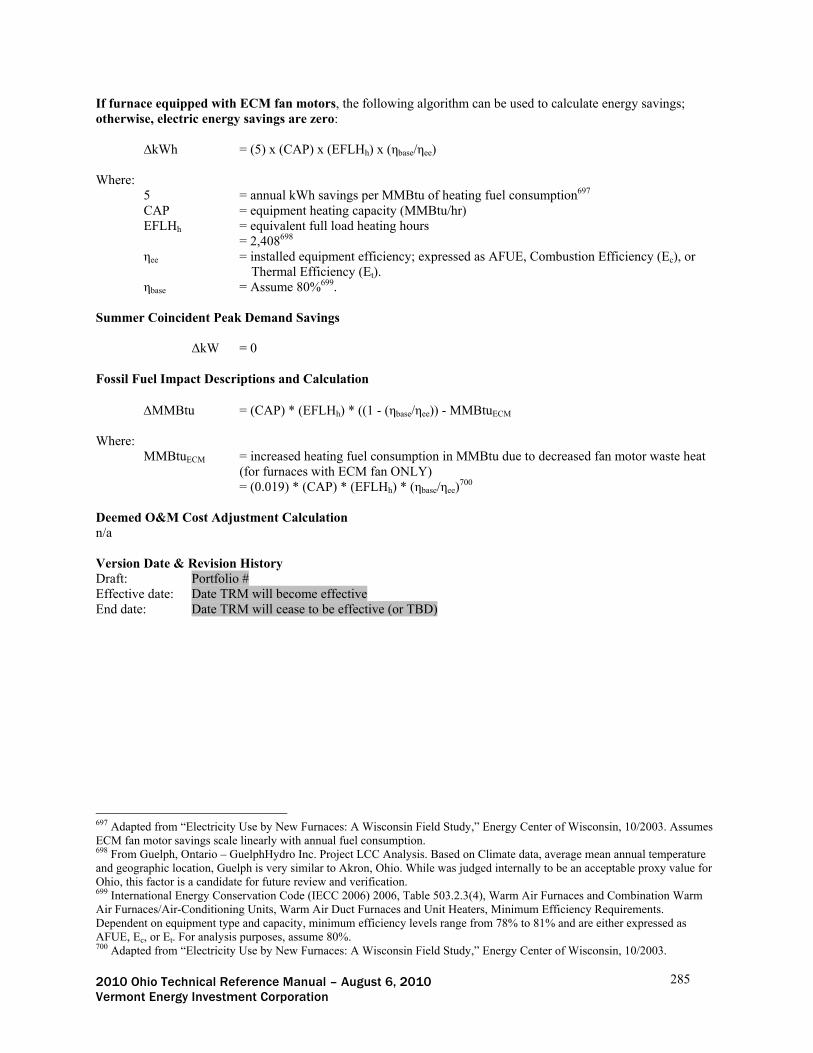
2010 Ohio Technical Reference Manual – August 6, 2010 285 Vermont Energy Investment Corporation
If furnace equipped with ECM fan motors, the following algorithm can be used to calculate energy savings; otherwise, electric energy savings are zero:
∆kWh = (5) x (CAP) x (EFLHh) x (ηbase/ηee)
Where:
5 = annual kWh savings per MMBtu of heating fuel consumption697 CAP = equipment heating capacity (MMBtu/hr) EFLHh = equivalent full load heating hours = 2,408698 ηee = installed equipment efficiency; expressed as AFUE, Combustion Efficiency (Ec), or
Thermal Efficiency (Et). ηbase = Assume 80%699.
Summer Coincident Peak Demand Savings ΔkW = 0
Fossil Fuel Impact Descriptions and Calculation MMBtu = (CAP) * (EFLHh) * ((1 - (ηbase/ηee)) - MMBtuECM Where:
MMBtuECM = increased heating fuel consumption in MMBtu due to decreased fan motor waste heat (for furnaces with ECM fan ONLY)
= (0.019) * (CAP) * (EFLHh) * (ηbase/ηee)700
Deemed O&M Cost Adjustment Calculation n/a Version Date & Revision History Draft: Portfolio # Effective date: Date TRM will become effective End date: Date TRM will cease to be effective (or TBD)
697 Adapted from “Electricity Use by New Furnaces: A Wisconsin Field Study,” Energy Center of Wisconsin, 10/2003. Assumes ECM fan motor savings scale linearly with annual fuel consumption. 698 From Guelph, Ontario – GuelphHydro Inc. Project LCC Analysis. Based on Climate data, average mean annual temperature and geographic location, Guelph is very similar to Akron, Ohio. While was judged internally to be an acceptable proxy value for Ohio, this factor is a candidate for future review and verification. 699 International Energy Conservation Code (IECC 2006) 2006, Table 503.2.3(4), Warm Air Furnaces and Combination Warm Air Furnaces/Air-Conditioning Units, Warm Air Duct Furnaces and Unit Heaters, Minimum Efficiency Requirements. Dependent on equipment type and capacity, minimum efficiency levels range from 78% to 81% and are either expressed as AFUE, Ec, or Et. For analysis purposes, assume 80%. 700 Adapted from “Electricity Use by New Furnaces: A Wisconsin Field Study,” Energy Center of Wisconsin, 10/2003.

2010 Ohio Technical Reference Manual – August 6, 2010 286 Vermont Energy Investment Corporation
High Efficiency Storage Tank Water Heater (Time of Sale, Retrofit – Early Replacement) Official Measure Code (Measure Number: X-X-X-X (Program name, End Use) Description Stand-alone, or tank-type heaters, run off natural gas. These water heaters consist of a storage tank with an attached heat source, in this case, a high-efficiency gas burner. They achieve energy savings through the use of efficient heating equipment and superior tank insulation. Definition of Efficient Equipment The efficient case is a natural gas-fired tank-type water heater exceeding the efficiency requirements as mandated by the International Energy Conservation Code (IECC) 2006, Table 504.2. Definition of Baseline Equipment The baseline condition is a gas-fired tank-type water heater meeting the efficiency requirements as mandated by the International Energy Conservation Code (IECC) 2006, Table 504.2. Deemed Savings for this Measure
Annual kWh Savings = 0
Summer Coincident Peak kW Savings = 0
Annual MMBtu Savings = [W x 8.33 x (Tout-Tin) x ((1/ηbase)-(1/ηee)) +
(STBYbase - STBYee) x 8760] / 1,000,000 Deemed Lifetime of Efficient Equipment 12 years701 Deemed Measure Cost $300702 Deemed O&M Cost Adjustments n/a Coincidence Factor n/a
REFERENCE SECTION
Calculation of Savings Energy Savings There are no expected energy savings associated with this measure Summer Coincident Peak Demand Savings There is no expected peak demand reduction associated with this measure.
701 Ibid. 702 Ibid.

2010 Ohio Technical Reference Manual – August 6, 2010 287 Vermont Energy Investment Corporation
Fossil Fuel Impact Descriptions and Calculation ∆MMBtu = [W x 8.33 x (Tout-Tin) x ((1/ηbase)-(1/ηee)) + (STBYbase - STBYee) x 8760] / 1,000,000 Where:
W = Annual water use for equipment (in gallons) = If actual water usage is unknown, assume 21,900703. 8.33 = weight in lbs of 1 gallon of water, or the Btus required to raise 1 gallon of water 1 ºF
Tout = water heater set point (ºF) = If unknown, assume 130 ºF704 Tin = water inlet temperature (ºF) = If unknown, assume 50ºF705
ηbase = rated efficiency of baseline water heater expressed as Energy Factor (EF) or Thermal Efficiency (Et
); see table below for values:
Equipment Type Size Category (Input) Subcategory
Performance Required706 (ηbase and STBYbase)
<= 75,000 Btu/h >= 20 gal EF = 0.67 - 0.0019V > 75,000 Btu/h and <= 155,000 Btu/h < 4,000 Btu/h/gal
Et = 80%, STBYbase = (Q / 800 + 110√V)
Storage water heaters, Gas
> 155,000 Btu/h < 4,000 Btu/h/gal Et = 80%, STBYbase = (Q / 800 + 110√V)
V = rated tank volume in gallons = Actual installed Q = nameplate input rate in Btu/hr = Actual installed ηee = rated efficiency of efficient water heater expressed as Energy Factor (EF) or Thermal
Efficiency (Et)
= Actual installed STBYbase = standby losses/hr of baseline water heater (Btu/hr); see table above for values. STBYee = standby losses/hr of efficient water heater (Btu/hr) = Actual installed (for unit rated with Energy Factor (EF), STBYbase = 0)
8760 = hours per year 1,000,000 = conversion factor (Btu/MMBtu)
Water Impact Descriptions and Calculation n/a Deemed O&M Cost Adjustment Calculation n/a Version Date & Revision History Draft: Portfolio # Effective date: Date TRM will become effective End date: Date TRM will cease to be effective (or TBD)
703 60 gallons a day for 365 days per year 704 NAHB Research Center, (2002). Performance Comparison of Residential Hot Water Systems. Prepared for: National Renewable Energy Laboratory, Golden, Colorado. 705 NAHB Research Center, (2002). Performance Comparison of Residential Hot Water Systems. Prepared for: National Renewable Energy Laboratory, Golden, Colorado. 706 International Energy Conservation Code (IECC 2006) 2006, Table 504.2, Minimum Performance of Water-Heating Equipment.

2010 Ohio Technical Reference Manual – August 6, 2010 288 Vermont Energy Investment Corporation
Tankless Water Heaters (Time of Sale, Retrofit – Early Replacement) Official Measure Code (Measure Number: X-X-X-X (Program name, End Use) Description This measure covers the installation of a natural gas-fired tankless or instantaneous water heater. Tankless water heaters essentially function like normal water heaters without the storage tank. When there is demand for hot water, the gas burner fires and heats water as it passes through the heater to the demand source. Because the water heater must heat water at the rate of flow through the device, tankless water heaters are not well suited to serve sources of significant demand. Tankless water heaters achieve savings by eliminating the standby losses that occur in stand-alone or tank-type water heaters. Definition of Efficient Equipment The efficient case is a tankless natural gas-fired water heater exceeding the efficiency requirements as mandated by the International Energy Conservation Code (IECC) 2006, Table 504.2. Definition of Baseline Equipment The baseline condition is a gas-fired tank-type water heater meeting the efficiency requirements as mandated by the International Energy Conservation Code (IECC) 2006, Table 504.2. Deemed Calculation for this Measure
Annual kWh Savings = 0 Summer Coincident Peak kW Savings = 0 Annual MMBtu Savings = W x 8.33 x (Tout-Tin) x [(1/ ηbase) – (1 / ηee)] x (STBYbase x
8760) / 1,000,000 Deemed Lifetime of Efficient Equipment 20 years707 Deemed Measure Cost 708 Full Installed Cost: $871.74 Incremental Material Cost: $433.72 Deemed O&M Cost Adjustments $9.60709 Coincidence Factor n/a
707 CenterPoint Energy – Triennial CIP/DSM Plan 2010-2012 Report 708 2008 Database for Energy-Efficiency Resources (DEER), Version 2008.2.05, “Cost Values and Summary Documentation”, California Public Utilities Commission, December 16, 2008 709 CenterPoint Energy – Triennial CIP/DSM Plan 2010-2012 Report

2010 Ohio Technical Reference Manual – August 6, 2010 289 Vermont Energy Investment Corporation
REFERENCE SECTION
Calculation of Savings Energy Savings There are no expected energy savings associated with this measure Summer Coincident Peak Demand Savings There is no expected peak demand reduction associated with this measure. Fossil Fuel Impact Descriptions and Calculation ∆MMBtu = W x 8.33 x (Tout-Tin) x [(1/ ηbase) – (1 / ηee)] x (STBYbase x 8760) / 1,000,000 Where:
W = Annual water use for equipment (in gallons) = If actual water usage is unknown, assume 21,900710. 8.33 = weight in lbs of 1 gallon of water, or the Btus required to raise 1 gallon of water 1 ºF
Tout = water heater set point (ºF) (demand temperature) = If unknown, assume 130 ºF711 Tin = water inlet temperature (ºF) = If unknown, assume 50ºF712
ηbase = rated efficiency of baseline water heater expressed as Energy Factor (EF) or Thermal Efficiency (Et
); see table below for values:
Equipment Type Size Category (Input) Subcategory
Performance Required713 (ηbase and STBYbase)
<= 75,000 Btu/h >= 20 gal EF = 0.67 - 0.0019V > 75,000 Btu/h and <= 155,000 Btu/h < 4,000 Btu/h/gal
Et = 80%, STBYbase = (Q / 800 + 110√V)
Storage water heaters, Gas
> 155,000 Btu/h < 4,000 Btu/h/gal Et = 80%, STBYbase = (Q / 800 + 110√V)
V = rated tank volume in gallons = Actual installed Q = nameplate input rate in Btu/hr = Actual installed ηee = rated efficiency of efficient water heater expressed as Energy Factor (EF) or Thermal
Efficiency (Et)
= Actual installed 1,000,000 = conversion factor (Btu/MMBtu)
STBYbase = standby losses/hr of baseline water heater (Btu/hr); see table above for values. Water Impact Descriptions and Calculation n/a Deemed O&M Cost Adjustment Calculation n/a
710 60 gallons a day for 365 days per year 711 NAHB Research Center, (2002). Performance Comparison of Residential Hot Water Systems. Prepared for: National Renewable Energy Laboratory, Golden, Colorado. 712 NAHB Research Center, (2002). Performance Comparison of Residential Hot Water Systems. Prepared for: National Renewable Energy Laboratory, Golden, Colorado. 713 International Energy Conservation Code (IECC 2006) 2006, Table 504.2, Minimum Performance of Water-Heating Equipment.

2010 Ohio Technical Reference Manual – August 6, 2010 290 Vermont Energy Investment Corporation
Version Date & Revision History Draft: Portfolio # Effective date: Date TRM will become effective End date: Date TRM will cease to be effective (or TBD)

2010 Ohio Technical Reference Manual – August 6, 2010 291 Vermont Energy Investment Corporation
Stack Damper (Retrofit – New Equipment) Official Measure Code (Measure Number: X-X-X-X (Efficient Products, HVAC End Use) Description This measure covers the installation of a servo-controlled, exhaust vent stack damper on a boiler. The vent damper should be installed in the flue pipe, between the heating equipment and the chimney. A stack damper works like a flue damper on a fireplace by reducing draft, improving comfort, and minimizing heat loss. The vent damper can either be controlled by a heat sensor installed directly in the vent stack or by a mechanical switch connected to the thermostat, which is wired to work in unison with the ignition control switch on the boiler.
In combustion appliances that are directly vented to the atmosphere, there is a decrease in operating efficiency during standby, start-up and shut-down. During these times, warm room air is drawn through the stack via the draft hood or dilution air inlet at a rate proportional to the stack height, diameter and outdoor temperature. The most air is drawn through the vent immediately after the appliance shuts off and the flue is still hot.
A vent damper can prevent residual heat from being drawn up the warm vent stack by closing itself. Vent dampers can also reduce the amount of air that passes through the furnace or boiler heat exchanger by regulating start-up exhaust pressure, which can increase operating efficiency by reducing the time needed to achieve steady-state operating conditions. Lastly, by reducing air infiltration in the building, vent dampers can help to retain humidity, which can improve comfort during periods of high heating degree days. Definition of Efficient Equipment The efficient equipment is a vent stack with a damper installed. Definition of Baseline Equipment The baseline condition is a vent stack with no stack damper installed. Deemed Calculation for this Measure
Annual kWh Savings = n/a Summer Coincident Peak kW Savings = n/a
Annual MMBtu Savings = 100 MMBtu714 Deemed Lifetime of Efficient Equipment 12 yrs715 Deemed Measure Cost $150716 Deemed O&M Cost Adjustments n/a Coincidence Factor n/a
714 CenterPoint Energy – Triennial CIP/DSM Plan 2010-2012 Report. Based on information published by Natural Resources Canada and the Minneapolis Energy Office, savings estimates for stack dampers range from to 0 to 9.5% of total boiler gas consumption. This implies that the boiler capacity assumed to determine the deemed savings value is quite large and may overstate savings for smaller boilers. If significant participation for this measure is realized, it is suggested that the deemed savings estimate be abandoned in favor of a deemed calculated approach. 715 CenterPoint Energy – Triennial CIP/DSM Plan 2010-2012 Report 716 Manufacturer research suggests a range of $80-$200 materials cost, depending on size, safety controls and motor quality, as well as 1-2 hours average install time.

2010 Ohio Technical Reference Manual – August 6, 2010 292 Vermont Energy Investment Corporation
REFERENCE SECTION
Calculation of Savings Energy Savings There are no expected energy savings associated with this measure Summer Coincident Peak Demand Savings There is no expected peak demand reduction associated with this measure. Baseline Adjustment n/a Fossil Fuel Impact Descriptions and Calculation MMBtu = 100 MMBtu Deemed O&M Cost Adjustment Calculation n/a Version Date & Revision History Draft: Portfolio # Effective date: Date TRM will become effective End date: Date TRM will cease to be effective (or TBD)

2010 Ohio Technical Reference Manual – August 6, 2010 293 Vermont Energy Investment Corporation
Natural Gas-Fired Infrared Heater (Time of Sale) Official Measure Code (Measure Number: X-X-X-X (Efficient Products, HVAC End Use) Description This measure covers the installation of a natural gas-fired infrared heater. Definition of Efficient Equipment An infrared heater heats primarily through radiation and conduction, as opposed to traditional forced-air space heaters which heat through convection. Infrared heaters are able to heat more efficiently because they directly heat the objects in the space, including the floor slab, which then radiate heat into the air space. With a forced hot air system, the heated air rises to the ceiling and stratifies, gradually working its way down to the floor level. The floor slab and equipment act as heat sinks causing the ceiling level to be much warmer than the floor area, which will cause the forced air system to work much harder to heat the same space. What is more, forced-air systems can experience drastic losses of heated air to ventilation air changes. There is also a negligible amount of electricity use (burner ignition and gas valve) compared to a forced-air system which requires large fans to move air around the conditioned space. Definition of Baseline Equipment The baseline equipment is a standard natural gas-fired convection space heater. Deemed Calculation for this Measure
Annual kWh Savings = n/a Summer Coincident Peak kW Savings = n/a
Annual MMBtu Savings = 11.4 MMBtu/year717 Deemed Lifetime of Efficient Equipment 15 yrs718 Deemed Measure Cost $920 (incremental cost)719 Deemed O&M Cost Adjustments n/a Coincidence Factor n/a
717 Based on engineering modeling by GSE in support of “Application of Columbia Gas of Ohio, Inc, to Establish Demand Side Management Programs for Residential and Commercial Consumers,” Filed with the Ohio Public Utilities Commission, Case No. 08-0833-GA-UNC, July 1, 2008. A review of savings assumptions used in Massachusetts indicates that this estimate is very conservative. The proposed value is only 85% of what is assumed for Massachusetts and should be considered for future study if this measure receives significant participation. 718 Ibid. 719 Ibid.

2010 Ohio Technical Reference Manual – August 6, 2010 294 Vermont Energy Investment Corporation
REFERENCE SECTION
Calculation of Savings Energy Savings There are no expected energy savings associated with this measure Summer Coincident Peak Demand Savings There is no expected peak demand reduction associated with this measure. Baseline Adjustment n/a Fossil Fuel Impact Descriptions and Calculation
∆MMBtu = 11.4 MMBtu/year Deemed O&M Cost Adjustment Calculation n/a Version Date & Revision History Draft: Portfolio # Effective date: Date TRM will become effective End date: Date TRM will cease to be effective (or TBD)

2010 Ohio Technical Reference Manual – August 6, 2010 295 Vermont Energy Investment Corporation
Energy Efficient Boiler (Time of Sale) Official Measure Code (Measure Number: X-X-X-X (Efficient Products, HVAC End Use) Description This measure covers the replacement of an irreparable existing boiler with a high efficiency, gas-fired steam or hot water boiler. High efficiency boilers achieve gas savings through the utilization of a sealed combustion chamber and multiple heat exchangers that remove a significant portion of the waste heat from flue gasses. Because multiple heat exchangers are used to remove waste heat from the escaping flue gasses, some of the flue gasses condense and must be drained. Definition of Efficient Equipment The efficient equipment is a natural gas-fired hot water or steam boiler exceeding the efficiency requirements as mandated by the International Energy Conservation Code (IECC) 2006, Table 503.2.3(5). Definition of Baseline Equipment The baseline equipment is a natural gas-fired boiler meeting the efficiency requirements as mandated by the International Energy Conservation Code (IECC) 2006, Table 503.2.3(5). Deemed Calculation for this Measure
Annual kWh Savings = 0
Summer Coincident Peak kW Savings = 0
Annual MMBtu Savings = (CAP) x (EFLHh) x (1 - (ηbase/ηee))
Deemed Lifetime of Efficient Equipment 20 years720 Deemed Measure Cost Incremental cost is estimated at $5,000721 Deemed O&M Cost Adjustments $0722 Coincidence Factor n/a
REFERENCE SECTION
Calculation of Savings Energy Savings There are no expected energy savings associated with this measure Summer Coincident Peak Demand Savings There is no expected peak demand reduction associated with this measure.
720 Based on engineering modeling by Michael Blasnik (M. Blasnik & Associates) in support of “Application of Columbia Gas of Ohio, Inc, to Establish Demand Side Management Programs for Residential and Commercial Consumers,” Filed with the Ohio Public Utilities Commission, Case No. 08-0833-GA-UNC, July 1, 2008 721 Ibid. 722 Ibid.
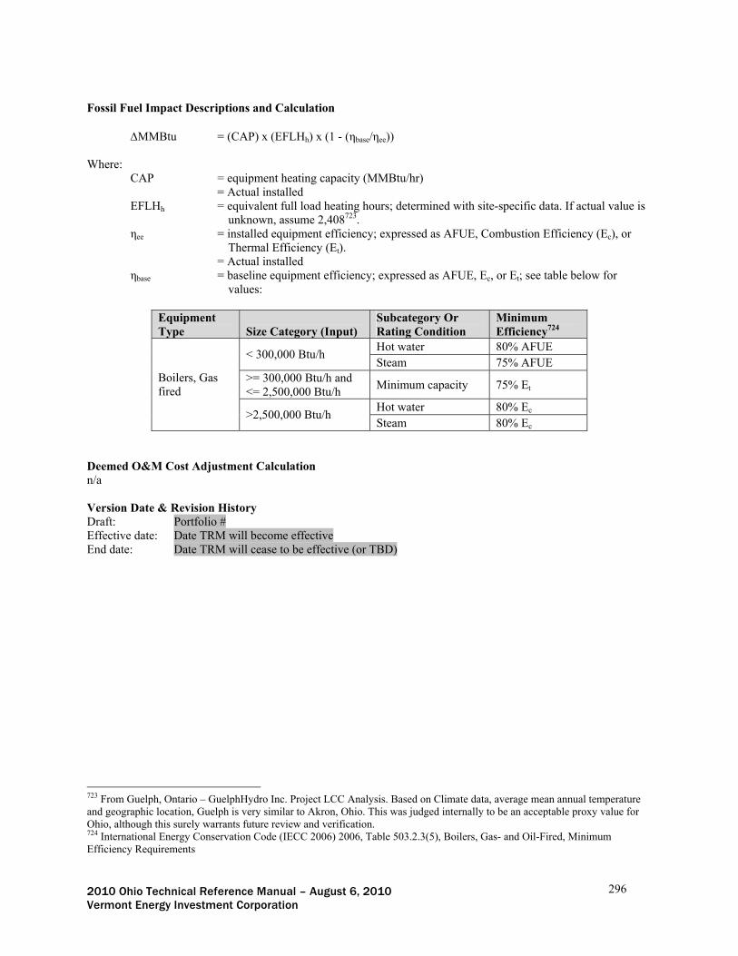
2010 Ohio Technical Reference Manual – August 6, 2010 296 Vermont Energy Investment Corporation
Fossil Fuel Impact Descriptions and Calculation MMBtu = (CAP) x (EFLHh) x (1 - (ηbase/ηee)) Where:
CAP = equipment heating capacity (MMBtu/hr) = Actual installed EFLHh = equivalent full load heating hours; determined with site-specific data. If actual value is
unknown, assume 2,408723. ηee = installed equipment efficiency; expressed as AFUE, Combustion Efficiency (Ec), or
Thermal Efficiency (Et). = Actual installed ηbase = baseline equipment efficiency; expressed as AFUE, Ec, or Et; see table below for
values:
Equipment Type Size Category (Input)
Subcategory Or Rating Condition
Minimum Efficiency724
Hot water 80% AFUE < 300,000 Btu/h
Steam 75% AFUE >= 300,000 Btu/h and <= 2,500,000 Btu/h
Minimum capacity 75% Et
Hot water 80% Ec
Boilers, Gas fired
>2,500,000 Btu/h Steam 80% Ec
Deemed O&M Cost Adjustment Calculation n/a Version Date & Revision History Draft: Portfolio # Effective date: Date TRM will become effective End date: Date TRM will cease to be effective (or TBD)
723 From Guelph, Ontario – GuelphHydro Inc. Project LCC Analysis. Based on Climate data, average mean annual temperature and geographic location, Guelph is very similar to Akron, Ohio. This was judged internally to be an acceptable proxy value for Ohio, although this surely warrants future review and verification. 724 International Energy Conservation Code (IECC 2006) 2006, Table 503.2.3(5), Boilers, Gas- and Oil-Fired, Minimum Efficiency Requirements

2010 Ohio Technical Reference Manual – August 6, 2010 297 Vermont Energy Investment Corporation
IV. Protocols for Custom Commercial & Industrial Projects
C&I Equipment Replacement – Custom Measure Analysis Protocol This protocol defines the requirements for analyzing and documenting commercial and industrial energy efficiency measures. It applies to custom measures filed under Utility Programs and those prepared for Mercantile Customers. This protocol addresses equipment replacement measures that are not covered by other analysis methodologies in the TRM. An equipment replacement project is defined as equipment replaced at the end of its rated service life, or when it is replaced due to failure, obsolescence or a need for increased capacity. If the project is replacing equipment prior to the end of its rated service life for the purpose of achieving energy savings, it is classified as Retrofit and the “C&I Retrofit – Custom Measure Analysis Protocol” should be used to guide analysis. This protocol is intended to address the energy impacts of the incremental energy efficiency improvements over what would have been installed as per applicable federal/state/local codes or standard industry practice. Projects that include duplex, redundant and/or spare equipment shall calculate the energy savings based only on the operating equipment and systems. This analysis protocol is supplemented by a glossary and an Analysis Template (Appendix B). Words used herein that are defined in the glossary are in italics. The Analysis Template is a tool that can guide applicants in preparing and presenting the documentation to support custom equipment replacement energy efficiency measure savings estimates. The Analysis Protocol is divided into four sections: Section 1: Project Information Section 2: Project Savings Section 3: Project Variables Section 4: Documentation and Metering Section 1: Project Information Project Title Provide a unique title for the project so that it is easily distinguishable from other projects prepared by the same customer and from projects with similar scope. Example: Company XYZ Building A - Compressed Air System Replacement. Customer Name Provide the name of the company undertaking the energy efficiency improvements. Customer Contact Provide the contact information including name, title, mailing address, phone, and email for the primary customer contact on this project. Site (Location) Provide the full address of the site at which the project is being implemented. If the customer has an additional business location that is involved with the project, include additional customer site information as needed. Sector/Industry Description and NAICS Code Describe the sector and industry in which the custom measure is being applied. Sectors include: Industrial, Commercial, Institutional, and Multi-family. Industry should specify the end use for commercial and institutional projects (e.g. office, restaurant, dormitory) and the specific industry for manufacturing projects725.
725 2007 NAICS; North American Industry Classification System; http://www.census.gov/cgi-bin/sssd/naics/naicsrch?chart=2007

2010 Ohio Technical Reference Manual – August 6, 2010 298 Vermont Energy Investment Corporation
Utility(ies) Information The name of the affected utility(ies) serving the customer. Provide all relevant account and meter information for electric and gas accounts and meters affected by the project. Program Identify the program under which this project will be submitted and why the project falls under the program. Projects submitted under existing utility programs should identify the program under which the project application will be filed and the utility-specific identifier for the project. Projects being submitted under the Mercantile Program should so indicate. Project/Technology Description Describe the energy using equipment and systems affected by the project in lay terms. Include specific information regarding industrial process technologies. For example: “Expand existing lab fume hoods by replacing two 10ft constant speed 10,000 CFM hoods with two 15ft modulating hoods controlled by smoke and temperature sensors.” Project Implementation Schedule Define the implementation schedule for the project, including start and completion dates. Measures Included in the Project All energy efficiency measures included in the project shall be clearly identified and savings calculations and estimates shall be clearly documented for each measure in accordance with this protocol. Affected Energy Sources (Electric, Gas, Other) Identify all affected energy sources (electric, gas, propane, oil, solar, etc.) for the project, provide a brief description of how the source energy use is affected and quantify the impacts in the analysis. Analysis Firm(s) and Contact(s) Provide information regarding the firm performing the engineering analysis of the custom project. Provide the name(s) of the contacts for the firm(s) and contact information including company name, individual(s) name, address, phone, and email. Section 2: Energy Consumption and Demand This section defines the requirements for calculating baseline and efficient case energy consumption and demand as well as the method for calculating savings. Calculations shall address all project variables in accordance with the requirements of Section 3 and undertake the analysis in accordance with the documentation and metering requirements in Section 4. The equations used in this protocol assume that the project has a single measure. If the project has multiple measures, these calculations shall be repeated for each measure in such a way as to capture interactive effects. Efficient Case
Efficient Technology Description and Documentation Describe the new technology, measure, and/or change in operations, and how it saves energy. Document any relevant efficiency codes or federal/state/local standards that apply to the proposed efficient equipment and the ratings of the measure equipment in comparison with applicable standards. If the efficient measure was the result of a process improvement that provides additional benefits, such as waste reduction, clearly describe all of the ways that the new process saves energy and resources. This can include reductions in areas such as waste heat, O&M costs, labor costs, water consumption, or process waste. Efficient Case Annual Energy Use Calculate the annual energy use for the proposed equipment using the methodologies outlined in this protocol and all referenced and applicable standards.

2010 Ohio Technical Reference Manual – August 6, 2010 299 Vermont Energy Investment Corporation
The total efficient energy use shall be calculated separately for each energy source (e.g. electric and gas) according to the following equations. For loads calculated from a regression analysis (e.g. kW vs. Temperature as described in Section 4) the following equation shall be used:
Where
Annual Efficient Energy Use - annual energy use with the efficiency improvement installed, calculated separately for each measure and each energy source (electric, gas).
Efficient Load (electric kW, gas therms) - efficient load for each system and subsystem
with operating condition j (as defined below). For example, efficient load will need to be calculated differently for staged condenser fans that have different operating hours or multiple pumps that operate at varying speeds.
Total Annual Operating – total annual operating hours for each system and subsystem
with operating condition j (as defined below). For loads calculated based on metering of full load or on equipment specifications:
where
Annual Efficient Energy Use - annual energy use with the efficiency improvement installed, calculated separately for each measure and each energy source (electric, gas).
Efficient Full Load - the maximum operating load of each efficient system and subsystem
with operating condition j (as defined below). Load Factor - fraction of Full Load for each efficient system and subsystem with
operating condition j (as defined below). Typically less than 1.00 unless the equipment was sized to run at 100% of rated capacity.
If needed, LF could be calculated from a regression curve kW and FULL LOAD for distinct operating conditions. This may arise when comparing efficient data with non-metered baseline LF ranges which are not based on a regression curve.
Total Annual Operating Hours – Total Annual Operating Hours for each system and
subsystem with operating condition j (as defined below).
System Condition - refers to each distinct combination of system mode, number of hours, full load demand, and load factor for each system or subsystem. Refer to example below.
Number of Terms – total Number of Terms needed to cover all conditions of affected
systems and subsystems.

2010 Ohio Technical Reference Manual – August 6, 2010 300 Vermont Energy Investment Corporation
Efficient Case Coincident Electric Demand (kW) Document the efficient case coincident electric demand for each measure according to one of the following equations: For variable loads:
Where
Average Efficient Load of all affected equipment during the Performance Hours
of 3-6 pm, weekday, non-holidays from June 1 – August 31 for a total of 195 hours. Includes non-operating time during the Performance Hours and is equal to total energy use during the Performance Hours divided by the total Performance Hours.
For constant loads or loads without metered data:
where
Average Coincident Efficient Load – Average Coincident Load of all affected efficient equipment during the Performance Hours of 3-6 pm, weekday, non-holidays from June 1 – August 31 for a total of 195 hours. Includes non-operating time during the Performance Hours.
Efficient Full Load - the maximum operating load of each efficient system and
subsystem during the Performance Hours with operating condition k (as defined below), exclusive of non operating time.
Load Factor - fraction of Full Load for each efficient system and subsystem with
operating condition k (as defined below). Typically less than 1.00 unless the equipment was sized to run at 100% of rated capacity.
Coincidence Factor - the Coincidence Factor is the fraction of time that each
efficient system and subsystem is operating during the Performance Hours for operating condition k (as defined below). The three typical conditions for CF are as follows: CF is unity if the equipment is continuously on during the Performance Hours; CF is zero for each system or subsystem that is not operating during the Performance Hours; otherwise, CF is the ratio of the ’on’ time to the total number of performance hours.
System Condition - refers to each distinct combination of the system mode, Full
Load demand, and Load Factor for each system or subsystem operating during the Performance Hours. Refer to example below.
Number of Terms – total Number of Terms needed to cover all operating modes
of affected systems and subsystems during Performance Hours.

2010 Ohio Technical Reference Manual – August 6, 2010 301 Vermont Energy Investment Corporation
The analysis shall include documentation of how the load varies during the Performance Hours. For constant load equipment, the analysis shall be based on the equipment load and operating schedule during the performance hours. For variable load equipment, the analysis shall address variations in equipment load and operating schedule during the performance hours. Additional analysis will typically be prepared to address the impact of the energy efficiency measure on customer peak demand. Such analysis is critical to calculating customer cost savings but should not be confused with the required calculation of the coincident demand during the performance hours.
Baseline Case Baseline Technology Methodology and Description Baseline for Equipment Replacement projects is the equipment meeting the level of efficiency required by State Code726, applicable Federal product efficiency standard727 or standard practices, whichever is most stringent, in place at the time of installation. If there is no applicable State code or Federal Standard then the methodology for establishing standard practice shall be documented in the M&V plan as described in PJM Manual 18B728 Section 8. The baseline description shall detail information regarding the baseline technology(ies) including make, model number, nameplate data and rated capacity of the equipment, operating schedule, and controls and how the baseline was determined.
Baseline Case Annual Energy Use Calculate the annual energy use for the baseline equipment and systems using the methodologies outlined in this protocol and all referenced and applicable standards. The total baseline energy use shall be calculated separately for each energy source (e.g. electric and gas) according to the following equations. For loads calculated from a regression analysis (e.g. kW vs. Temperature as described in Section 4) the following equation shall be used:
Where
Annual Baseline Energy Use - Annual Energy Use for baseline equipment calculated separately for each measure and each energy source (electric, gas).
Baseline Load (electric kW, gas therms) - Baseline Load for each system and subsystem
with operating condition j (as defined below). For example, Baseline Load will need to be calculated differently for staged condenser fans that have different operating hours or multiple pumps that operate at varying speeds.
Total Annual Operating Hours – Total Annual Operating Hours for each system and
subsystem with operating condition j (as defined below).
For loads calculated based on equipment specifications and metering of baseline operating conditions including load factor and operating hours:
726 International Code Council, 2007 Ohio Building Code; http://publicecodes.citation.com/st/oh/st/b2v07/index.htm?bu2=undefined 727 ANSI/ASHRAE/IESNA Standard 90.1-2004, ISSN 1041-2336; www.ashrae.org 728 PJM Manual 18B: Energy Efficiency Measurement and Verification, Rev. 0, Effective date: April 23, 2009; PJM M&V Manual approved 4_09.pdf

2010 Ohio Technical Reference Manual – August 6, 2010 302 Vermont Energy Investment Corporation
where
Annual Baseline Energy Use - Annual Energy Use for baseline equipment calculated separately for each measure and each energy source (electric, gas).
Baseline Full Load - the maximum operating load of each baseline system and subsystem
with operating condition j (as defined below).
Load Factor - fraction of Full Load for each baseline system and subsystem with operating condition j (as defined below). Typically less than 1.00 unless the equipment was sized to run at 100% of rated capacity.
Total Annual Operating Hours – Total Annual Operating Hours for each system and
subsystem with operating condition j (as defined below).
System Condition - refers to each distinct combination of system mode, number of hours, Full Load demand, and Load Factor for each system or subsystem. Refer to example below.
Number of Terms – total Number of Terms needed to cover all conditions of affected
systems and subsystems. Baseline Case Full Load Demand Document the baseline case coincident electric demand for each measure according to one of the following equations: For variable loads:
Where
Average Baseline Load of all affected equipment during the Performance Hours
of 3-6 pm, weekday, non-holidays from June 1 – August 31 for a total of 195 hours. Includes non-operating time during the Performance Hours and is equal to total energy use during the Performance Hours divided by the total Performance Hours.
For constant loads:
where
Average Coincident Baseline Load – average coincident load of all affected
baseline equipment during the Performance Hours of 3-6 pm, weekday, non-holidays from June 1 – August 31 for a total of 195 hours. Includes non-operating time during the Performance Hours.

2010 Ohio Technical Reference Manual – August 6, 2010 303 Vermont Energy Investment Corporation
Baseline Full Load - the maximum operating load of each baseline system and
subsystem during the Performance Hours with operating condition k (as defined below), exclusive of non operating time.
Load Factor - fraction of Full Load for each baseline system and subsystem with operating condition k (as defined below). Typically less than 1.00 unless the equipment was sized to run at 100% of rated capacity.
Coincidence Factor - the Coincidence Factor is the fraction of time that each
baseline system and subsystem is operating during the Performance Hours for operating condition k (as defined below). The three typical conditions for CF are as follows: CF is unity if the equipment is continuously on during the Performance Hours; CF is zero for each system or subsystem that is not operating during the Performance Hours; otherwise, CF is the ratio of the ’on’ time to the total number of performance hours.
System Condition - refers to each distinct combination of the system mode, Full
Load demand, and Load Factor for each system or subsystem operating during Performance Hours. Refer to example below.
Number of Terms – total Number of Terms needed to cover all operating modes
of affected systems and subsystems during Performance Hours. The analysis shall include documentation of how the load varies during the Performance Hours. For constant load equipment, the analysis shall be based on the equipment load and operating schedule during the Performance Hours. For variable load equipment, the analysis shall address variations in equipment load and operating schedule during the Performance Hours. Additional analysis will typically be prepared to address the impact of the baseline equipment on customer peak demand. Such analysis is critical to calculating customer cost savings but should not be confused with the required calculation of the coincident demand during the Performance Hours.
Savings Savings shall be calculated from the efficient case and baseline case energy and demand calculations from above. Address project variables as described in Section 3 and aggregate so that interactive effects are accurately accounted for in the analysis.
Annual Energy Savings (kWh for electrical, therms for gas)
where
and are defined above.
Coincident Electrical Demand Reduction (kW) =

2010 Ohio Technical Reference Manual – August 6, 2010 304 Vermont Energy Investment Corporation
where
and are defined above. Section 3: Project Variables Accurately capturing and documenting the variables that affect annual energy use and savings as well as those affecting peak period demand coincidence are critical elements in developing meaningful and reliable energy savings estimates. The savings analysis shall consider and address the variables over the life of the measure for both the baseline and efficient case. Uncertainty in variables shall be quantified and the savings analysis shall clearly demonstrate transparency and reasonableness in definition and application of variables affecting energy savings729. The variables below are common to many custom energy analyses. Document the variables that affect the energy use of the project for both the baseline and efficient scenarios and delineate the methods used for data collection (i.e. meter data, trend logs, manufacturer data, customer interviews, production logs, etc.) and any uncertainty associated with the values used in the analysis. ALL savings calculations must be normalized to reflect consistent application of the assumed variables for the project under both baseline and post installation conditions over the full range of operating conditions for the affected systems. Load Characterization Accurate characterization of the baseline and efficient energy use involves a comprehensive analysis of all variables that affect the loads over the analysis period. Concepts that are commonly used in performing energy analysis are discussed below. In all cases it is the intent of this document to require that the variations in load due to all factors (weather, production, schedule, etc) are accounted for in the analysis.
Load Shape The load shape reflects variations in load over the course of a year, with specific attention paid to the peak periods defined by the affected utility and/or regional transmission organization. The load shape should capture the expected period at which the load will operate at full load (full load hours) as well as all part load and non-operating or standby-modes. For highly variable loads, development of an 8760 load shape will increase the accuracy of the analysis and the reliability of claimed demand reductions during peak periods730.
Load Factor Load factor is the ratio of maximum energy demand to the average electric demand for the affected end use. Analysis of loads across a representative sample of operating conditions can generate a single load factor for constant load applications. For variable load applications, a series of load factors must be developed to accurately represent the variations in energy use under the variety of loading conditions that occur over the range of operating cycles in a typical calendar year. Variable load analysis shall address the variations in load factor over a one year period for all dependent variables. Peak Load Factor Peak Load Factor describes the variation between the maximum connected load of the equipment and the highest actual load of the equipment. In some cases the peak load factor is unity. For oversized equipment it is frequently less than one. In some rare instances where equipment is operated above its rated load, the peak load factor may be greater than one.
729 Anne Arquit Niederberger, PhD, A+B International (2005), Baseline Methodologies for Industrial End-Use Efficiency Presentation. Presented at World Bank; Anne_Arquit_Niederberger_Industry_EE_CDM_Dec_05.xls 730 Patil, Yogesh, et. al. (Aug, 2009) “Taking Engineering Savings to the Next Level, presented at IEPEC 2009 http://www.ers-inc.com/images/articles/Papers/takingsavingstonextlevel.pdf

2010 Ohio Technical Reference Manual – August 6, 2010 305 Vermont Energy Investment Corporation
Coincidence Factor Coincidence Factor is the coincidence of the demand savings during the Peak Performance Hours. For custom Equipment Replacement measures, the average coincident demand, including non-operational hours, is typically determined by metering the post-installation condition and deriving the Coincidence Factor for the pre-installation condition from the metered data. However, in some cases, the use of a known or predetermined published Coincidence Factor, such as measure specific coincidence factors identified in other sections of the TRM is acceptable. An example of Coincidence Factor derivation from metered data would be a stepped demand device such as a high efficiency compressor. Based on post-installation metering, a Coincidence Factor can be calculated and applied to the baseline equipment when the baseline operating schedule is the same as the efficient operating schedule. In this case, the Coincidence Factor is defined as the ratio of average metered demand for the Peak Performance Hours and max ‘equipment on’ demand when operating. If the equipment is operating continuously for the full peak performance hours, then the coincidence factor is 1.00.
Operating Conditions Characterize all variable operating conditions that affect the load over the analysis period. Typical operating variables are outlined below. Additional factors may be required to accurately characterize variability in equipment operations and the energy savings resulting from energy efficiency measures over the full range of operating conditions.
Operating Hours Establish the baseline and post-installation operating hours for all affected equipment using logging, metering, and/or DDC trending for a representative period of not less than one week. Where pre- and post-installation operating schedules are the same, use of pre- or post-logging of operating hours to prepare the analysis is adequate. Address all variations in operating schedule over an annual operating cycle including, but not limited to weekends, holidays, and shift or occupancy changes that are a result in cyclical changes in operations over the course of a year. (For example retail applications may have longer operating hours in November and December). Project analysis shall clearly identify all operating, non-operating, and standby hours, the related loads, the periods for which those conditions apply and the basis for the assumptions in the analysis. Special attention should be paid that the hours of Coincident Peak (3:00 – 6:00 weekdays from June 1 through August 31) are detailed. Weather For weather-dependent projects, the analysis shall address the impact of annual weather, including temperature, humidity, and solar incidence (where applicable) on energy consumption. All savings (energy and demand) should be normalized to the TMY3 (Typical Meteorological Year) that corresponds to the nearest TMY3 weather site using modeling and/or regression analysis. TMY3 data should be obtained from National Renewable Energy Laboratory (NREL731) and used as the 8760 weather file to model and/or normalize annual energy use for weather dependent measures. Modeling tools, such as eQuest732, currently use TMY2 data. TMY3 data is based on more-recent and more accurate data and is available for many more locations; TMY3 data is available for over 1,000 locations, where TMY2 data is available for fewer than 300 locations. Projects with hourly correlation of metered or utility billed usage to local weather conditions should be done using National Oceanic and Atmospheric Administration (NOAA733) or NREL data. NOAA weather data is available for a small fee downloadable from the Internet and is typically the most accurate and complete historical local weather data set. NREL data is free but typically has some gaps in the data and is emailed in response to specific requests. Caution should be exercised when using non-government generated weather data as it may not meet accepted standards for quality and accuracy.
731 Typical Meteorological Data (TMY3) - http://rredc.nrel.gov/solar/old_data/nsrdb/1991-2005/tmy3/ 732 DOE2 eQuest simulation software - http://www.doe2.com/equest/ 733 NOAA local weather data - http://cdo.ncdc.noaa.gov/qclcd/QCLCD?prior=N

2010 Ohio Technical Reference Manual – August 6, 2010 306 Vermont Energy Investment Corporation
Production Project analysis shall reflect variations in production over the cycles within the analysis period. Variations can include such things as the number of shifts or changes in quantity or type of product manufactured. For industrial process measures, production documentation shall normalize energy use based on the energy intensity of the process (i.e. energy use per unit of output) over the lifetime of the measure for both the baseline and efficient cases. Measurement of output should be based on physical measures of output (i.e. ton of steel or paper) and capture variations in both production levels and manufactured product types over the analysis period for both the calculated baseline and the metered efficient case734. Post-installation metering shall include documentation of production output during metering periods; work with plant personnel to ensure logged production data accurately reflects changes in production over the metering period. Assumptions regarding economic climate, changes in production levels, and shifts all affect calculated energy savings over the life of the measures. Develop reasonable assumptions regarding these variables and ensure the application of these variables is clearly identified in both the analysis and project documentation. Identify the uncertainty introduced into the energy savings estimates as a result of these assumptions.
Controls Control settings and level of control shall be accounted for in the analysis. Clearly document the control points that affect energy use, the control setpoints, sequence of operation and accuracy of controls that would have been used in the baseline case. Clearly document the changes in these conditions for the efficient case. Include relevant information such as commissioning of control points, potential manual overrides of control sequences and anticipated control point calibration over the life of the measure. Occupancy Where occupancy affects energy use and varies over time, capture the variations in occupancy and their effects over the analysis period. At a minimum there is typically an ‘occupied’ and an ‘unoccupied’ mode for most facilities. Assumptions regarding economic climate and shifts in hours of occupancy affect calculated energy savings over the life of the measures. Develop reasonable assumptions regarding these variables and ensure the application of these variables is clearly identified in both the analysis and project documentation. Identify the uncertainty introduced into the energy savings estimates as a result of these assumptions
Interactive Effects Analysis shall explicitly account for interactive effects between measures. For projects that include both prescriptive and custom measures, account for the energy use reduction from the prescriptive measure in the custom measure analysis. As prescriptive measures include interactive effects themselves, document the methodology that is used to ensure that savings from the interactive effects are only accounted for once in the claimed savings. One common set of interactive effects is the impact of electrical energy efficiency measures within a facility on that facility’s heating and/or cooling load. These shall be addressed as follows:
Waste Heat For efficiency upgrades that reduce the rejection of waste heat into air conditioned spaces (i.e. evaporator fans in a refrigerated enclosure), quantify the reduction in heat rejection735 and the associated cooling reduction.
734 Ruth, Michael, Lawrence Berkeley National Laboratory, et. al. (2001) A Process-Step Benchmarking Approach to Energy Use at Industrial Facilities: Examples from the Iron and Steel and Cement Industries; Process_Step_Benchmarking_ACEEE_LBNL-50444.doc 735 2009 ASHRAE Handbook, Fundamentals, Chapter 18, page 18.3.

2010 Ohio Technical Reference Manual – August 6, 2010 307 Vermont Energy Investment Corporation
Heating Increase For efficiency upgrades that reduce the rejection of waste heat into heated spaces, quantify the additional heating fuel required to offset the change and maintain temperature within the space14. The analysis shall address heating system efficiency and include basis for assumptions regarding fossil fuel increases.
For projects with multiple measures, the procedure for interactive effects is to calculate savings for the longest lived measure first, then consider that measure’s impact on the next longest-lived measure, and so on. This is because a short-lived measure can affect savings from a long-lived measure, but only for part of its life. Since tracking system limitations require that annual measure savings remain constant for all years, this is the only way to ensure proper lifetime savings and total resource benefits are captured. Measure Life Document both the life of the baseline and efficient case equipment. The efficient case analysis is typically performed over the lifetime of the efficiency measures. Where the analysis period and the efficiency measure life are not the same, describe the rationale for the analysis period and assumptions regarding replacement equipment for measures with lives that are shorter than the analysis period. Persistence Persistence factors may be used to reduce lifetime measure savings in recognition that initial engineering estimates of annual savings may not persist long term736. The persistence factor accounts for uncertainties and for normal operations over the life of the measure. For instance if energy efficient motors are installed as part of a process and the customer’s standard procedure is to have motors rewound upon failure, the energy efficiency associated with the efficient motor would only persist until the expected time when the motor is rewound. Persistence is also affected by measures being removed or failing prior to the end of its normal engineering lifetime, improper maintained over the life of the measure, control overrides or loss of calibration (controls only), etc. Related Variables: Related variables are those which are not included in the energy and demand calculations, but may be required for project cost-effectiveness screening by the utility(ies). Document the following variables for the project:
Operation &Maintenance (O&M) Impacts Where O&M practices would have resulted in changes to the baseline during the analysis period, account for such practices in the establishment of baseline and efficiency case energy use.
Water Consumption Impacts Quantify any changes in water consumption attributable to the project.
Cost Document the cost of each measure. Include invoices, bids and other documentation to substantiate project cost data. Identify portions of the cost which are for equipment being purchased for redundancy or backup and will not generate savings in the project. Related costs such as the costs for audits, design, engineering, permits, fees or M&V should be reported separately from the costs associated with the design and installation of energy efficiency improvements.
Other Variables As needed - clearly document all variables affecting the energy use of the project that have not been covered in this document. Section 4: Documentation and Metering
736 Efficiency Vermont Technical Reference User Manual (TRM) Measure Savings Algorithms and Cost Assumptions, February 19, 2010

2010 Ohio Technical Reference Manual – August 6, 2010 308 Vermont Energy Investment Corporation
Documentation and metering of custom projects are essential to developing reliable energy savings and Coincident Electrical Demand reduction claims.737 The following guidelines support the accurate estimation of energy and demand savings. Data and Metering
Document how the data will be collected and utilized in the savings analysis in a Measurement and Verification (M&V) Plan. The Custom Analysis Template (Appendix B) can be used as a tool to document the M&V plan and analysis738. Metering for Equipment Replacement projects is typically conducted post-installation to establish the Coincidence Factor, operating hours and Load Factor. Where measures include a control component, metering of these factors in the baseline condition is necessary to accurately establish the baseline. Interval and Utility Data Utility interval data is typically not useful in analyzing equipment replacement projects because the baseline condition is not represented in the utility billing data. For completed mercantile projects in existing facilities, project documentation shall include two - three years of utility billing information from years PRIOR to measure installation and up to three years of utility data post installation in accordance with PUCO requirements. Meter Data Accuracy of all metering and measurement equipment shall be documented in the M&V Plan. Document the metering methods including equipment type, location of metering equipment, and equipment set up process, as well as metering duration and timeframe for which data was collected. Capture all variables that affect energy use of the measures during the metering period as outlined in Section 3. Describe how the metered data, including timeframe and operational factors at the time of metering, relate to the operational conditions that occur over the course of a year. Provide photographs of meter installation and clear documentation of meter numbers and the associated equipment names of the equipment being metered in the project documentation. Meter data files should clearly identify the equipment to which the meter data applies. For variable loads, three-phase power data loggers shall be used to collect electrical power data for systems and subsystems of the custom measure739. For constant loads, accurate spot reading of the load coupled with runtime logging is an acceptable metering methodology. Temperature and time of use loggers can be used to meter proxy variables, equipment status, and runtimes. Ensure that proxy variable metering yields calculated kW values in compliance with PJM740 Section 11 requirements. Three-phase power data loggers shall record: amperage, voltage, power factor, and kW on all phases as well as the totals for each variable. All electrical power metering shall adequately account for harmonics741. Logging shall capture equipment load under representative operating conditions. The time period of logging shall be adequate to represent variations in load that will occur over the analysis period. Where feasible, use metering or data logging to capture variables affecting load during the metering period. Where variables cannot be captured using meters or data loggers, institute and clearly document a method for accurately capturing variables, validating non-metered data, and aligning it with metered data. Metering periods shall be a minimum of one week, including a weekend, for constant load equipment and
737 Parlin, Kathryn, et. al. (August, 2009 IEPEC) “Demand Reduction in the Forward Capacity Market, Verifying the Efficiency Power Plant” 738 IPMVP, Volume III, Part I, January 2006, Chapter 3, page 7 through 10, and PJM Manual 18B, April 2009, section 2, page 10 through 14 739 PJM Manual 18B: Energy Efficiency Measurement and Verification, Rev. 0, Section 11, Effective date: April 23, 2009; PJM M&V Manual approved 4_09.pdf 740 PJM Manual 18B: Energy Efficiency Measurement and Verification, Rev. 0, Section 11, Effective date: April 23, 2009; PJM M&V Manual approved 4_09.pdf 741 PJM Manual 18B: Energy Efficiency Measurement and Verification, Rev. 0, Section 11, Effective date: April 23, 2009; PJM M&V Manual approved 4_09.pdf

2010 Ohio Technical Reference Manual – August 6, 2010 309 Vermont Energy Investment Corporation
at least two weeks, including weekends, for variable load equipment, but as noted above, must be long enough to capture representative variations in load expected over the entire analysis period. Integrating/averaging three-phase power meters are desirable. Power metering accuracy requirements are outlined in PJM Manual 18B742 and RLW Analytics Review of ISO New England Measurement and Verification Equipment Requirements743. Metering intervals shall be the smallest time interval that will permit acquisition of data over the minimum required metering period. For short-cycling or modulating systems, 30-second or 1-minute data intervals are preferred, with a maximum recommended interval of 5 minutes. For constant load systems, the metering interval can be longer. No metering interval should exceed 15 minutes. Clearly document how meter intervals and meter periods capture the expected load variations for the project. Meters and data loggers shall be synchronized to the NIST time clock, and differences between the time at the facility and the NIST time setting should be noted when the meters are installed. DDC/PLC Monitor Data Use of DDC and PLC monitoring software trends in the analysis is acceptable provided that the sensors are calibrated on site using calibrated test instruments and the results documented by the energy analyst before the metering period commences. Review and submission of annual equipment calibration records for DDC sensors and metering equipment is a less desirable, but acceptable alternative to calibration of DDC equipment as part of the project. Timestamps for trends should be set up to coincide with those of any concurrently deployed data loggers to enable accurate data analysis. Load Profiles For measures with well established and reliable load profiles, the load profile can be a useful tool for determining savings. Load profiles are most reliable when used for common measures in typical applications, such as office lighting projects. Typically, load profiles should not be relied on where project peak demand savings exceed 20 kW.
General Procedures for Data Analysis
Data Cleaning
It is usually necessary to ‘clean’ the raw data before proceeding with the analysis. The following data cleaning tasks are typically required. Ensure that the timestamps match between datasets (e.g. for concurrent kW and temperature datasets), and that any gaps in the data which are not representative of typical operation have been addressed by interpolation or other means. Interpolated or derived data shall be flagged, and the method used to fill in data gaps shall be described. Note that in preparing the data for use in the 8760 analysis, there will likely be blocks of time during the metering period that will be analyzed differently. For example, during regular business hours a load may be temperature dependent and the data will be analyzed using a regression analysis of kW vs. outdoor air temperature; whereas the same piece of equipment on the weekend may have a constant standby load and is thus schedule driven and non-temperature dependent on the weekends. Different blocks of the 8760 hours in a year will be populated from the separate analyses of the distinct blocks of meter data.
742 PJM Manual 18B: Energy Efficiency Measurement and Verification, Rev. 0, Effective date: April 23, 2009; PJM M&V Manual approved 4_09.pdf 743 RLW Analytics, Review of ISO New England Measurement and Verification Equipment Requirements, Final Report, April 24, 2008 Prepared for: Northeast Energy Efficiency Partnerships’ Evaluation and State Program Working Group; RLW Metering Report.pdf

2010 Ohio Technical Reference Manual – August 6, 2010 310 Vermont Energy Investment Corporation
Annualization and Analysis Approach
The recommended approach to annualization of meter data and savings calculations is an 8760 analysis744. This approach inherently captures seasonality and peak period variability on an hourly basis and is therefore more accurate than other traditional methods such as binned analysis. Typical approaches to analyzing custom measures include:
Demand vs. temperature analysis for temperature dependent measures. Daily operating profiles for schedule-driven measures Cyclical production profiles for production-related measures
These methods should address part load performance, and may employ different metrics such as:
Demand vs. percent capacity Demand/Ton vs. percent capacity Demand vs. hours Demand per ton, pound, cubic foot or quantity
Calculations
Clearly document all calculations. Indicate how the meter data is used in the analysis and why this is appropriate for the measure. Meter data used in the analysis shall be clearly distinguished from data not used in the analysis.
Computer simulation of energy efficiency measures based on meter data using 8760 hourly simulation models such as eQuest, or customized spreadsheet analysis or other energy analysis tools can be employed to calculate energy savings. The algorithms of the modeling software must be designed to address the custom measure. Minimum documentation requirements include model output reports stating unmet load hours for the baseline and efficient case, hourly energy use and demand, and electronic copies of the model or spreadsheet analysis files. Annual kWh and therms for baseline and efficient cases shall be the annualized and normalized per the equations in Section 2 using the methods described above. Coincident Electric Demand for baseline and efficient cases shall be calculated from post-installation meter data as the average demand over the Performance Hours as indicated in Section 2. Calculation documentation shall include definitions and reference sources for all variables and assumed factors in Section 3.
Documentation Analysis shall be documented with comprehensive, well labeled supporting information including, but not limited to:
Manufacturer literature documenting connected load for both the baseline and the installed equipment or manufacturer data documenting the information necessary to calculate peak demand (such as horsepower, voltage, efficiency, etc.) shall be included in the project documentation. Manufacturer data shall be clearly marked to indicate the specific equipment model number and data that is applicable to the project and used in the calculations.
Where citing nameplate ratings in the analysis, provide documentation of the ratings.
744 Patil, Yogesh, et. al. (Aug, 2009) “Taking Engineering Savings to the Next Level, presented at IEPEC 2009; http://www.ers-inc.com/images/articles/Papers/takingsavingstonextlevel.pdf

2010 Ohio Technical Reference Manual – August 6, 2010 311 Vermont Energy Investment Corporation
Manufacturer data shall be adjusted to reflect actual site operating conditions. Document calculation of the adjusted connected load reflecting metered on site conditions.
Reporting The following metrics and details shall be reported:
All information required in this protocol M&V Plan/Analysis Template
Regression R2 values for fits of demand vs. proxy variables.
Cleaned meter data (raw data shall be included as an appendix) clearly indicating which data was used in the savings analysis
Discussion of approach to anomalies, outliers, interpolations and extrapolations in the analysis
Assessment of the level of uncertainty associated with the energy and demand calculated savings.
Project commissioning can reduce energy use and is recommended. If the project was commissioned, submit a copy of the commissioning report.

2010 Ohio Technical Reference Manual – August 6, 2010 312 Vermont Energy Investment Corporation
C&I Retrofit – Custom Measure Analysis Protocol This protocol defines the requirements for analyzing and documenting commercial and industrial energy efficiency measures. It applies to custom measures filed under Utility Programs and those prepared for Mercantile Customers. This protocol addresses retrofit measures that are not covered by other analysis methodologies in the TRM. A retrofit project is defined as equipment replacement prior to the end of its rated service life in order to achieve energy savings. Where equipment is replaced due to failure or for other reasons (such as obsolescence or a need for increased capacity), the project is classified as Equipment Replacement and the “C&I Equipment Replacement – Custom Measure Analysis Protocol” should be used to guide analysis. This protocol is intended to address the energy impacts of the operating energy efficiency improvements. Projects that include duplex, redundant and/or spare equipment shall calculate the energy savings based only on the operating equipment and systems. This analysis protocol is supplemented by a glossary and an Analysis Template (Appendix B). Words used herein that are defined in the glossary are in italics. The Analysis Template is a tool that can guide applicants in preparing and presenting the documentation to support custom retrofit energy efficiency measure savings estimates. The Analysis Protocol and Analysis Template are divided into four sections: Section 1: Project Information Section 2: Project Savings Section 3: Project Variables Section 4: Documentation and Metering Section 1: Project Information Project Title Provide a unique title for the project so that it is easily distinguishable from other projects prepared by the same customer and from projects with similar scope. Example: Company XYZ Building A - Compressed Air System Improvements. Customer Name Provide the name of the company undertaking the energy efficiency improvements. Customer Contact Provide the contact information including name, title, mailing address, phone, and email for the primary customer contact on this project. Site (Location) Provide the full address of the site at which the project is being implemented. If the customer has an additional business location that is involved with the project, include additional customer site information as needed. Sector/Industry Description and NAICS Code Describe the sector and industry in which the custom measure is being applied. Sectors include: Industrial, Commercial, Institutional, and Multi-family. Industry should specify the end use for commercial and institutional projects (e.g. office, restaurant, dormitory) and the specific industry for manufacturing projects745. Utility(ies) Information The name of the affected utility(ies) serving the customer. Provide all relevant account and meter information for electric and gas accounts and meters affected by the project. Program
745 2007 NAICS; North American Industry Classification System; http://www.census.gov/cgi-bin/sssd/naics/naicsrch?chart=2007

2010 Ohio Technical Reference Manual – August 6, 2010 313 Vermont Energy Investment Corporation
Identify the program under which this project will be submitted and why the project falls under the program. Projects submitted under existing utility programs should identify the program under which the project application will be filed and the utility-specific identifier for the project. Projects being submitted under the Mercantile Program should so indicate. Project/Technology Description Describe the energy using equipment and systems affected by the project in lay terms. Include specific information regarding industrial process technologies. For example: “Replace two 10ft constant speed 10,000 CFM fume hoods with modulating fume hoods controlled by smoke and temperature sensors.” Project Implementation Schedule Define the implementation schedule for the project, including start and completion dates. Measures Included in the Project All energy efficiency measures included in the project shall be clearly identified and savings calculations and estimates shall be clearly documented for each measure in accordance with this protocol. Affected Energy Sources (Electric, Gas, Other) Identify all affected energy sources (electric, gas, propane, oil, solar, etc.) for the project, provide a brief description of how the source energy use is affected and quantify the impacts in the analysis. Analysis Firm(s) and Contact(s) Provide information regarding the firm performing the engineering analysis of the custom project. Provide the name(s) of the contacts for the firm(s) and contact information including company name, individual(s) name, address, phone, and email. Section 2: Energy Consumption and Demand This section defines the requirements for calculating baseline and efficient case energy consumption and demand as well as the method for calculating savings. Calculations shall address all project variables in accordance with the requirements of Section 3 and undertake the analysis in accordance with the documentation and metering requirements in Section 4. The equations used in this protocol assume that the project has a single measure. If the project has multiple measures, these calculations shall be repeated for each measure in such a way as to capture interactive effects. Efficient Case
Efficient Technology Description and Documentation Describe the new technology, measure, and/or change in operations, and how it saves energy. Document any relevant efficiency codes or federal/state/local standards that apply to the proposed efficient equipment and the ratings of the measure equipment in comparison with applicable standards. If the efficient measure was the result of a process improvement that provides additional benefits, such as waste reduction, clearly describe all of the ways that the new process saves energy and resources. This can include reductions in areas such as waste heat, O&M costs, labor costs, water consumption, or process waste. Efficient Case Annual Energy Use Calculate the annual energy use for the proposed equipment using the methodologies outlined in this protocol and all referenced and applicable standards. The total efficient energy use shall be calculated separately for each energy source (e.g. electric and gas) according to the following equations. For loads calculated from a regression analysis (e.g. kW vs. Temperature as described in Section 4) the following equation shall be used:

2010 Ohio Technical Reference Manual – August 6, 2010 314 Vermont Energy Investment Corporation
where
Annual Efficient Energy Use - annual energy use with the efficiency improvement installed, calculated separately for each measure and each energy source (electric, gas).
Efficient Load (electric kW, gas therms) - efficient load for each system and subsystem
with operating condition j (as defined below). For example, efficient load will need to be calculated differently for staged condenser fans that have different operating hours or multiple pumps that operate at varying speeds.
Total Annual Operating – total annual operating hours for each system and subsystem
with operating condition j (as defined below). For loads calculated based on metering of full load or on equipment specifications:
where
Annual Efficient Energy Use - annual energy use with the efficiency improvement installed, calculated separately for each measure and each energy source (electric, gas).
Efficient Full Load - the maximum operating load of each efficient system and subsystem
with operating condition j (as defined below).
Load Factor - fraction of full load for each efficient system and subsystem with operating condition j (as defined below). Typically less than 1.00 unless the equipment was sized to run at 100% or rated capacity.
If needed, LF could be calculated from a regression curve kW and FULL LOAD for distinct operating conditions. This may arise when comparing efficient data with non-metered baseline LF ranges which are not based on a regression curve.
Total Annual Operating Hours – total annual operating hours for each system and
subsystem with operating condition j (as defined below).
System Condition - refers to each distinct combination of system mode, number of hours, full load demand, and load factor for each system or subsystem. Refer to example below.
Number of Terms – total number of terms needed to cover all conditions of affected
systems and subsystems.

2010 Ohio Technical Reference Manual – August 6, 2010 315 Vermont Energy Investment Corporation
Efficient Case Coincident Electric Demand (kW) Document the efficient case coincident electric demand for each measure according to one of the following equations: For variable loads:
Where
Average Efficient Load of all affected equipment during the Performance Hours
of 3-6 pm, weekday, non-holidays from June 1 – August 31 for a total of 195 hours. Includes non-operating time during the Performance Hours and is equal to total energy use during the Performance Hours divided by the total Performance Hours.
For constant loads or loads without metered data:
where
Average Coincident Efficient Load – Average Coincident Load of all affected
efficient equipment during the Performance Hours of 3-6 pm, weekday, non-holidays from June 1 – August 31 for a total of 195 hours. Includes non-operating time during the Performance Hours.
Efficient Full Load - the maximum operating load of each efficient system and
subsystem during the Performance Hours with operating condition k (as defined below), exclusive of non operating time.
Load Factor - fraction of Full Load for each efficient system and subsystem with
operating condition k (as defined below). Typically less than 1.00 unless the equipment was sized to run at 100% of rated capacity.
Coincidence Factor - the Coincidence Factor is the fraction of time that each
efficient system and subsystem is operating during the Performance Hours for operating condition k (as defined below). The three typical conditions for CF are as follows: CF is unity if the equipment is continuously on during the Performance Hours; CF is zero for each system or subsystem that is not operating during the Performance Hours; otherwise, CF is the ratio of the ’on’ time to the total number of performance hours.
System Condition - refers to each distinct combination of the system mode, Full
Load demand, and Load Factor for each system or subsystem operating during the Performance Hours. Refer to example below.
Number of Terms – total Number of Terms needed to cover all operating modes
of affected systems and subsystems during Performance Hours.
2010 Ohio Technical Reference Manual – August 6, 2010 316 Vermont Energy Investment Corporation
The analysis shall include documentation of how the load varies during the Performance Hours. For constant load equipment, the analysis shall be based on the equipment load and operating schedule during the performance hours. For variable load equipment, the analysis shall address variations in equipment load and operating schedule during the performance hours. Additional analysis will typically be prepared to address the impact of the energy efficiency measure on customer peak demand. Such analysis is critical to calculating customer cost savings but should not be confused with the required calculation of the coincident demand during the performance hours.
Baseline Case
Baseline Technology Methodology and Description Energy efficiency retrofit projects involve the replacement of existing equipment prior to the end of its useful life in order to achieve energy savings. Therefore, the existing equipment may be used to establish the project baseline. The analysis must account for the remaining life of the existing equipment, and if the analysis period extends beyond the remaining life of the existing equipment, the analysis shall account for increases in efficiency that would have occurred through autonomous efficiency improvements or equipment replacement that would have occurred at the end of the existing equipment life in the absence of early retirement. The baseline description shall detail the baseline technology(ies) affected by the measure; including make, model number, nameplate information, and equipment rated capacity, condition, age, lifetime, usage, operating schedule, and controls. The baseline shall also account for upgrades to the equipment that would have occurred during the analysis period absent the early retirement of the equipment. Retrofit of industrial processes typically yield multiple benefits including energy efficiency, increased throughput, reduced waste, improved product quality, new product features, etc. Because of the multiple benefits derived from industrial process improvements, the characterization of these measures does not cleanly fall into either the retrofit or equipment replacement category. In order to establish a rigorous industrial process retrofit baseline, the following should be considered:
Derived Baseline – based on documented Industry and Applicant Practice (as described below), the engineer performing the analysis shall develop a reasonable project baseline. Clearly describe why the baseline and characterization of the project as retrofit is appropriate and demonstrate how the derived baseline accounts for autonomous upgrades in practice over the analysis period.
Current Industry Practice – document current industry practice using articles from industry journals, EIA industry specific energy intensity figures,746 and independent industry specific studies. Where information regarding industry practice is provided by manufacturers who sell production equipment within the industry, it shall be supported by independent research.
Applicant Practice – document the corporate practices of the applicant through annual reports, published papers, internal memos, and other documents that indicate the business practices of the applicant relative to current practice in the industry. Document the practices and equipment within the facility receiving the upgrade. For instance, if an injection molding manufacturer is replacing hydraulic machines with electric machines on an annual basis, using the hydraulic equipment as baseline may not be representative of the actual baseline. For production equipment replacements, a Process Integration Study747 is a strong tool in documenting the project’s focus on energy efficiency and the optimization of energy use.748
746 Department of Energy, Energy Information Administration, Manufacturing Energy Consumption Survey, http://www.eia.doe.gov/emeu/mecs/contents.html 747 Natural Resources Canada, Process Integration, A Systematic Approach for Optimisation of Industrial Processes, http://canmetenergy-canmetenergie.nrcan-rncan.gc.ca/fichier.php/codectec/En/2009-046/2009-046_en.pdf 748 Department of Energy, Industrial Efficiency Report, 1993, http://www.fas.org/ota/reports/9330.pdf
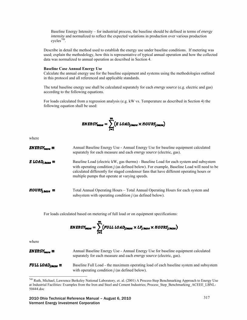
2010 Ohio Technical Reference Manual – August 6, 2010 317 Vermont Energy Investment Corporation
Baseline Energy Intensity – for industrial process, the baseline should be defined in terms of energy intensity and normalized to reflect the expected variations in production over various production cycles749.
Describe in detail the method used to establish the energy use under baseline conditions. If metering was used; explain the methodology, how this is representative of typical annual operation and how the collected data was normalized to annual operation as described in Section 4.
Baseline Case Annual Energy Use Calculate the annual energy use for the baseline equipment and systems using the methodologies outlined in this protocol and all referenced and applicable standards. The total baseline energy use shall be calculated separately for each energy source (e.g. electric and gas) according to the following equations. For loads calculated from a regression analysis (e.g. kW vs. Temperature as described in Section 4) the following equation shall be used:
where
Annual Baseline Energy Use - Annual Energy Use for baseline equipment calculated separately for each measure and each energy source (electric, gas).
Baseline Load (electric kW, gas therms) - Baseline Load for each system and subsystem
with operating condition j (as defined below). For example, Baseline Load will need to be calculated differently for staged condenser fans that have different operating hours or multiple pumps that operate at varying speeds.
Total Annual Operating Hours – Total Annual Operating Hours for each system and
subsystem with operating condition j (as defined below). For loads calculated based on metering of full load or on equipment specifications:
where
Annual Baseline Energy Use - Annual Energy Use for baseline equipment calculated separately for each measure and each energy source (electric, gas).
Baseline Full Load - the maximum operating load of each baseline system and subsystem
with operating condition j (as defined below).
749 Ruth, Michael, Lawrence Berkeley National Laboratory, et. al. (2001) A Process-Step Benchmarking Approach to Energy Use at Industrial Facilities: Examples from the Iron and Steel and Cement Industries; Process_Step_Benchmarking_ACEEE_LBNL-50444.doc

2010 Ohio Technical Reference Manual – August 6, 2010 318 Vermont Energy Investment Corporation
Load Factor - fraction of Full Load for each baseline system and subsystem with
operating condition j (as defined below). Typically less than 1.00 unless the equipment was sized to run at 100% of rated capacity.
Total Annual Operating Hours – Total Annual Operating Hours for each system and
subsystem with operating condition j (as defined below).
System Condition - refers to each distinct combination of system mode, number of hours, Full Load demand, and Load Factor for each system or subsystem. Refer to example below.
Number of Terms – total Number of Terms needed to cover all conditions of affected
systems and subsystems. Baseline Case Full Load Demand Document the baseline case coincident electric demand for each measure according to one of the following equations: For variable loads:
Where Average Baseline Load of all affected equipment during the Performance Hours
of 3-6 pm, weekday, non-holidays from June 1 – August 31 for a total of 195 hours. Includes non-operating time during the Performance Hours and is equal to total energy use during the Performance Hours divided by the total Performance Hours.
For constant loads or loads without metered data:
where
Average Coincident Baseline Load – average coincident load of all affected
baseline equipment during the Performance Hours of 3-6 pm, weekday, non-holidays from June 1 – August 31 for a total of 195 hours. Includes non-operating time during the Performance Hours.
Baseline Full Load - the maximum operating load of each baseline system and
subsystem during the Performance Hours with operating condition k (as defined below), exclusive of non operating time.
Load Factor - fraction of Full Load for each baseline system and subsystem with operating condition k (as defined below). Typically less than 1.00 unless the equipment was sized to run at 100% of rated capacity.

2010 Ohio Technical Reference Manual – August 6, 2010 319 Vermont Energy Investment Corporation
Coincidence Factor - the Coincidence Factor is the fraction of time that each baseline system and subsystem is operating during the Performance Hours for operating condition k (as defined below). The three typical conditions for CF are as follows: CF is unity if the equipment is continuously on during the Performance Hours; CF is zero for each system or subsystem that is not operating during the Performance Hours; otherwise, CF is the ratio of the ’on’ time to the total number of performance hours.
System Condition - refers to each distinct combination of the system mode, Full Load demand, and Load Factor for each system or subsystem operating during Performance Hours. Refer to example below.
Number of Terms – total Number of Terms needed to cover all operating modes
of affected systems and subsystems during Performance Hours. The analysis shall include documentation of how the load varies during the Performance Hours. For constant load equipment, the analysis shall be based on the equipment load and operating schedule during the Performance Hours. For variable load equipment, the analysis shall address variations in equipment load and operating schedule during the Performance Hours.
Additional analysis will typically be prepared to address the impact of the baseline equipment on customer peak demand. Such analysis is critical to calculating customer cost savings but should not be confused with the required calculation of the coincident demand during the Performance Hours. Savings Savings shall be calculated from the efficient case and baseline case energy and demand calculations from above. Address project variables as described in Section 3 and aggregate so that interactive effects are accurately accounted for in the analysis.
Annual Energy Savings (kWh for electrical, therms for gas)
where
and are defined above.
Coincident Electrical Demand Reduction (kW) =
where
and are defined above.
Section 3: Project Variables Accurately capturing and documenting the variables that affect annual energy use and savings as well as those affecting peak period demand coincidence are critical elements in developing meaningful and reliable energy savings estimates. The savings analysis shall consider and address the variables over the life of the measure for both

2010 Ohio Technical Reference Manual – August 6, 2010 320 Vermont Energy Investment Corporation
the baseline and efficient case. Uncertainty in variables shall be quantified and the savings analysis shall clearly demonstrate transparency and reasonableness in definition and application of variables affecting energy savings750. The variables below are common to many custom energy analyses. Document the variables that affect the energy use of the project for both the baseline and efficient scenarios and delineate the methods used for data collection (i.e. meter data, trend logs, manufacturer data, customer interviews, production logs, etc.) and any uncertainty associated with the values used in the analysis. ALL savings calculations must be normalized to reflect consistent application of the assumed variables for the project under both baseline and post installation conditions over the full range of operating conditions for the affected systems. Load Characterization Accurate characterization of the baseline and efficient energy use involves a comprehensive analysis of all variables that affect the loads over the analysis period. Concepts that are commonly used in performing energy analysis are discussed below. In all cases it is the intent of this document to require that the variations in load due to all factors (weather, production, schedule, etc) are accounted for in the analysis.
Load Shape The load shape reflects variations in load over the course of a year, with specific attention paid to the peak periods defined by the affected utility and/or regional transmission organization. The load shape should capture the expected period at which the load will operate at full load (full load hours) as well as all part load and non-operating or standby-modes. For highly variable loads, development of an 8760 load shape will increase the accuracy of the analysis and the reliability of claimed demand reductions during peak periods751.
Load Factor Load factor is the ratio of maximum energy demand to the average electric demand for the affected end use. Analysis of loads across a representative sample of operating conditions can generate a single load factor for constant load applications. For variable load applications, a series of load factors must be developed to accurately represent the variations in energy use under the variety of loading conditions that occur over the range of operating cycles in a typical calendar year. Variable load analysis shall address the variations in load factor over a one year period for all dependent variables. Peak Load Factor Peak load factor describes the variation between the maximum connected load of the equipment and the highest actual load of the equipment. In some cases the peak load factor is unity. For oversized equipment it is frequently less than one. In some rare instances where equipment is operated above its rated load, the peak load factor may be greater than one.
Coincidence Factor Coincidence Factor is the coincidence of the demand savings during the peak performance hours. For custom measures, the average coincident demand, including non-operational hours, is typically directly determined by metering the pre- and post-installation condition and a coincidence factor is not used in the calculations. However, in some cases, the use of a known or predetermined published coincidence factor to calculate the coincident peak reduction for a project may be appropriate. Another example of the use of an explicit coincidence factor arises in cases where the baseline demand was not metered and the efficient demand was metered. For a stepped demand device such as a high efficiency compressor, for example, a coincidence factor can be calculated and applied to the baseline equipment to address the fact that the baseline operating schedule used in the calculations should be the same as the efficient operating schedule. In this case, the coincidence factor is defined as the ratio of average metered
750 Anne Arquit Niederberger, PhD, A+B International (2005), Baseline Methodologies for Industrial End-Use Efficiency Presentation. Presented at World Bank; Anne_Arquit_Niederberger_Industry_EE_CDM_Dec_05.xls 751 Patil, Yogesh, et. al. (Aug, 2009) “Taking Engineering Savings to the Next Level, presented at IEPEC 2009 http://www.ers-inc.com/images/articles/Papers/takingsavingstonextlevel.pdf

2010 Ohio Technical Reference Manual – August 6, 2010 321 Vermont Energy Investment Corporation
demand for the peak performance hours and max ‘equipment on’ demand when operating. If the equipment is operating continuously for the full peak performance hours, then the coincidence factor is 1.00.
Operating Conditions Characterize all variable operating conditions that affect the load over the analysis period. Typical operating variables are outlined below. Additional factors may be required to accurately characterize variability in equipment operations and the energy savings resulting from energy efficiency measures over the full range of operating conditions.
Operating Hours Establish the baseline and post-installation operating hours for all affected equipment using logging, metering, and/or DDC trending for a representative period of not less than one week. Address all variations in operating schedule over an annual operating cycle including, but not limited to weekends, holidays, and shift or occupancy changes that are a result in cyclical changes in operations over the course of a year. (For example retail applications may have longer operating hours in November and December). Project analysis shall clearly identify all operating, non-operating, and standby hours, the related loads, the periods for which those conditions apply and the basis for the assumptions in the analysis. Special attention should be paid that the hours of Coincident Peak (3:00 – 6:00 weekdays from June 1 through August 31) are detailed. Weather For weather-dependent projects, the analysis shall address the impact of annual weather, including temperature, humidity, and solar incidence (where applicable) on energy consumption. All savings (energy and demand) should be normalized to the TMY3 (Typical Meteorological Year) that corresponds to the nearest TMY3 weather site using modeling and/or regression analysis. TMY3 data should be obtained from National Renewable Energy Laboratory (NREL752) and used as the 8760 weather file to model and/or normalize annual energy use for weather dependent measures. Modeling tools, such as eQuest753, currently use TMY2 data. TMY3 data is based on more-recent and more accurate data and is available for many more locations; TMY3 data is available for over 1,000 locations, where TMY2 data is available for fewer than 300 locations. Projects with hourly correlation of metered or utility billed usage to local weather conditions should be done using National Oceanic and Atmospheric Administration (NOAA754) or NREL data. NOAA weather data is available for a small fee downloadable from the Internet and is typically the most accurate and complete historical local weather data set. NREL data is free but typically has some gaps in the data and is emailed in response to specific requests. Caution should be exercised when using non-government generated weather data as it may not meet accepted standards for quality and accuracy. Production Project analysis shall reflect variations in production over the cycles within the analysis period. Variations can include such things as the number of shifts or changes in quantity or type of product manufactured. For industrial process measures, production documentation shall normalize energy use based on the energy intensity of the process (i.e. energy use per unit of output) over the lifetime of the measure for both the baseline and efficient cases. Measurement of output should be based on physical measures of output (i.e. ton of steel or paper) and capture variations in both production levels and manufactured product types over the analysis period for both the baseline and efficient case755. For metered projects, document production output during metering periods; work with plant personnel to ensure logged production data accurately reflects changes in production over the metering period.
752 Typical Meteorological Data (TMY3) - http://rredc.nrel.gov/solar/old_data/nsrdb/1991-2005/tmy3/ 753 DOE2 eQuest simulation software - http://www.doe2.com/equest/ 754 NOAA local weather data - http://cdo.ncdc.noaa.gov/qclcd/QCLCD?prior=N 755 Ruth, Michael, Lawrence Berkeley National Laboratory, et. al. (2001) A Process-Step Benchmarking Approach to Energy Use at Industrial Facilities: Examples from the Iron and Steel and Cement Industries; Process_Step_Benchmarking_ACEEE_LBNL-50444.doc

2010 Ohio Technical Reference Manual – August 6, 2010 322 Vermont Energy Investment Corporation
Assumptions regarding economic climate, changes in production levels, and shifts all affect calculated energy savings over the life of the measures. Develop reasonable assumptions regarding these variables and ensure the application of these variables is clearly identified in both the analysis and project documentation. Identify the uncertainty introduced into the energy savings estimates as a result of these assumptions. Process flow charting for manufacturing and production is recommended to clarify energy use and demand impacts for each stage in the process756.
Controls Control settings and level of control shall be accounted for in the analysis. Clearly document the baseline control points that affect energy use, the control setpoints, sequence of operation and accuracy of controls. Clearly document the changes in these conditions for the efficient case. Include relevant information such as commissioning of control points, potential manual overrides of control sequences and anticipated control point calibration over the life of the measure. Occupancy Where occupancy affects energy use and varies over time, capture the variations in occupancy and their effects over the analysis period. At a minimum there is typically an ‘occupied’ and an ‘unoccupied’ mode for any facility. Assumptions regarding economic climate and shifts in hours of occupancy affect calculated energy savings over the life of the measures. Develop reasonable assumptions regarding these variables and ensure the application of these variables is clearly identified in both the analysis and project documentation. Identify the uncertainty introduced into the energy savings estimates as a result of these assumptions
Interactive Effects Analysis shall explicitly account for interactive effects between measures. For projects that include both prescriptive and custom measures, account for the energy use reduction from the prescriptive measure in the custom measure analysis. As prescriptive measures include interactive effects themselves, it will be necessary to remove the interactive effects from the prescriptive measure before including the energy use reduction in the custom measure analysis. Document the methodology that is used to ensure that savings from the interactive effects are only accounted for once in the claimed savings. Interactive effects should be accounted for even if the technologies involved in the interactive effects are not the subject of energy efficiency improvements or claims under other programs, otherwise savings for custom measures may be overclaimed. The energy analyst should be aware of and request information about other changes or maintenance at the facility that may not be directly related to the custom measure project, or any other claimed project, and shall account for these changes in the analysis if appropriate. One common set of interactive effects is the impact of electrical energy efficiency measures within a facility on that facility’s heating and/or cooling load. These shall be addressed as follows:
Waste Heat For efficiency upgrades that reduce the rejection of waste heat into air conditioned spaces (i.e. evaporator fans in a refrigerated enclosure), quantify the reduction in heat rejection757 and the associated cooling reduction.
Heating Increase For efficiency upgrades that reduce the rejection of waste heat into heated spaces, quantify the additional heating fuel required to offset the change and maintain temperature within the space14. The analysis shall address heating system efficiency and include basis for assumptions regarding fossil fuel increases.
756 Doty, Commercial Energy Auditing Reference Handbook, p. 65 757 2009 ASHRAE Handbook, Fundamentals, Chapter 18, page 18.3.
2010 Ohio Technical Reference Manual – August 6, 2010 323 Vermont Energy Investment Corporation
For projects with multiple measures, the procedure for interactive effects is to calculate savings for the longest lived measure first, then consider that measure’s impact on the next longest-lived measure, and so on. This is because a short-lived measure can affect savings from a long-lived measure, but only for part of its life. Since tracking system limitations require that annual measure savings remain constant for all years, this is the only way to ensure proper lifetime savings and total resource benefits are captured. As an example; calibrating DDC controls can increase savings at the time of chiller replacement. Since DDC control calibration has a relatively short measure life, the DDC calibration will affect the savings of the new chiller only for the first few years of its lifetime. When the calibration measure expires, the consumption of the new chiller will increase and the savings associated with the chiller measure will decrease for the remainder of the chiller’s lifetime. If DDC calibration is calculated first, the chiller savings in the project will be overstated. Measure Life Document both the life of the baseline and efficient case equipment. If the baseline equipment measure life does not extend over the entire analysis period, the analysis shall include assumptions regarding replacement of baseline equipment at the end of its life. The efficient case analysis is typically performed over the lifetime of the efficiency measures. Where the analysis period and the efficiency measure life are not the same, describe the rationale for the analysis period and assumptions regarding replacement equipment for measures with lives that are shorter than the analysis period. Persistence Persistence factors may be used to reduce lifetime measure savings in recognition that initial engineering estimates of annual savings may not persist long term758. The persistence factor accounts for uncertainties and for normal operations over the life of the measure. For instance if energy efficient motors are installed as part of a process and the customer’s standard procedure is to have motors rewound upon failure, the energy efficiency associated with the efficient motor would only persist until the expected time when the motor is rewound. Persistence is also affected by measures being removed or failing prior to the end of its normal engineering lifetime, improper maintained over the life of the measure, control overrides or loss of calibration (controls only), etc. Related Variables: Related variables are those which are not included in the energy and demand calculations, but may be required for project cost-effectiveness screening by the utility(ies). Document the following variables for the project:
Operation &Maintenance (O&M) Impacts Where O&M practices would have resulted in changes to the baseline during the analysis period, account for such practices in the establishment of baseline and efficiency case energy use.
Water Consumption Impacts Quantify any changes in water consumption attributable to the project.
Cost Document the cost of each measure. Include invoices, bids and other documentation to substantiate project cost data. Identify portions of the cost which are for equipment being purchased for redundancy or backup and will not generate savings in the project. Related costs such as the costs for audits, design, engineering, permits, fees or M&V should be reported separately from the costs associated with the design and installation of energy efficiency improvements.
Other Variables As needed - clearly document all variables affecting the energy use of the project that have not been covered in this document. Section 4: Documentation and Metering
758 Efficiency Vermont Technical Reference User Manual (TRM) Measure Savings Algorithms and Cost Assumptions, February 19, 2010

2010 Ohio Technical Reference Manual – August 6, 2010 324 Vermont Energy Investment Corporation
Documentation and metering of custom projects are essential to developing reliable energy savings and peak demand reductions claims.759 The following guidelines support the accurate estimation of energy and demand savings. Data and Metering
Document how the data will be collected and utilized in the savings analysis in a Measurement and Verification (M&V) Plan. The Custom Analysis Template (Appendix B) can be used as a tool to document the M&V plan and analysis760. Interval and Utility Data Utility interval data may be used in the analysis where available and applicable. Interval data is deemed applicable when the order of magnitude of the custom measure can be distinguished from the other loads on the meter. If the load on the utility meter is highly variable, the custom measure would need to be a larger portion of the overall load in order for the savings to be determined from the utility data. Typically interval data is available in 15 minute increments; the shortest period available for interval data should be used in the analysis. Where interval data is used, the analysis shall follow the requirements of IPMVP Option C – Whole Building Analysis761. For measures which affect gas usage only, utility data is typically the primary means of quantifying savings. However, use of upstream metering equipment such as flow meters is encouraged to improve the accuracy of gas savings calculations. For completed mercantile projects in existing facilities, analysis shall include two - three years of utility billing information from years PRIOR to measure installation and up to three years of utility data post- installation in accordance with PUCO requirements. Meter Data Accuracy of all metering and measurement equipment shall be documented in the M&V Plan. Document the metering methods including equipment type, location of metering equipment, and equipment set up process, as well as metering duration and timeframe for which data was collected. Capture all variables that affect energy use of the measures during the metering period as outlined in Section 3. Describe how the metered data, including timeframe and operational factors at the time of metering, relate to the operational conditions that occur over the course of a year. Provide photographs of meter installation and clear documentation of meter numbers and the associated equipment names of the equipment being metered in the project documentation. Meter data files should clearly identify the equipment to which the meter data applies. For variable loads, three-phase power data loggers shall be used to collect electrical power data for systems and subsystems of the custom measure762. For constant loads, accurate spot reading of the load coupled with runtime logging is an acceptable metering methodology. Temperature and time of use loggers can be used to meter proxy variables, equipment status, and runtimes. Ensure that proxy variable metering yields calculated kW values in compliance with PJM Section 11 requirements. Three-phase power data loggers shall record: amperage, voltage, power factor, and kW on all phases as well as the totals for each variable. All electrical power metering shall adequately account for
759 Parlin, Kathryn, et. al. (August, 2009 IEPEC) “Demand Reduction in the Forward Capacity Market, Verifying the Efficiency Power Plant” 760 IPMVP, Volume III, Part I, January 2006, Chapter 3, page 7 through 10, and PJM Manual 18B, April 2009, section 2, page 10 through 14 761International Performance Measure and Verification Protocol Concepts and Practices for Determining Energy Savings in New Construction, Volume III, Part 1, January 2006. 762 PJM Manual 18B: Energy Efficiency Measurement and Verification, Rev. 0, Section 11, Effective date: April 23, 2009; PJM M&V Manual approved 4_09.pdf

2010 Ohio Technical Reference Manual – August 6, 2010 325 Vermont Energy Investment Corporation
harmonics763. Logging shall capture equipment load under representative operating conditions. The time period of logging shall be adequate to represent variations in load that will occur over the analysis period. Where feasible, use metering or data logging to capture variables affecting load during the metering period. Where variables cannot be captured using meters or data loggers, institute and clearly document a method for accurately capturing variables, validating non-metered data, and aligning it with metered data. Metering periods shall be a minimum of one week, including a weekend, for constant load equipment and at least two weeks, including weekends, for variable load equipment, but as noted above, must be long enough to capture representative variations in load expected over the entire analysis period. Integrating/averaging three phase power meters are desirable. Power metering accuracy requirements are outlined in PJM Manual 18B764 and RLW Analytics Review of ISO New England Measurement and Verification Equipment Requirements765. Metering intervals shall be the smallest time interval that will permit acquisition of data over the minimum required metering period. For short-cycling or modulating systems, 30-second or 1-minute data intervals are preferred, with a maximum recommended interval of 5 minutes. For constant load systems, the metering interval can be longer. No metering interval should exceed 15 minutes. Clearly document how meter intervals and meter periods capture the expected load variations for the project. Meters and data loggers shall be synchronized to the NIST time clock, and differences between the time at the facility and the NIST time setting should be noted when the meters are installed. DDC/PLC Monitor Data Use of DDC and PLC monitoring software trends in the analysis is acceptable provided that the sensors are calibrated on site using calibrated test instruments and the results documented by the energy analyst before the metering period commences. Review and submission of annual equipment calibration records for DDC sensors and metering equipment is a less desirable, but acceptable alternative to calibration of DDC equipment as part of the project. Timestamps for trends should be set up to coincide with those of any concurrently deployed data loggers to enable accurate data analysis. Load Profiles For measures with well established and reliable load profiles, the load profile can be a useful tool for determining savings. Load profiles are most reliable when used for common measures in typical applications, such as office lighting projects. Typically, load profiles should not be relied on where project peak demand savings exceed 20 kW.
General Procedures for Data Analysis
Data Cleaning
It is usually necessary to ‘clean’ the raw data before proceeding with the analysis. The following data cleaning tasks are typically required. Ensure that the timestamps match between datasets (e.g. for concurrent kW and temperature datasets), and that any gaps in the data which are not representative of typical operation have been addressed by interpolation or other means. Interpolated or derived data shall be flagged, and the method used to fill in data gaps shall be described. Note that in preparing the data for use in the 8760 analysis, there will likely be blocks of time during the metering period that will be analyzed differently. For example, during regular business hours, a load may
763 PJM Manual 18B: Energy Efficiency Measurement and Verification, Rev. 0, Section 11, Effective date: April 23, 2009; PJM M&V Manual approved 4_09.pdf 764 PJM Manual 18B: Energy Efficiency Measurement and Verification, Rev. 0, Effective date: April 23, 2009; PJM M&V Manual approved 4_09.pdf 765 RLW Analytics, Review of ISO New England Measurement and Verification Equipment Requirements, Final Report, April 24, 2008 Prepared for: Northeast Energy Efficiency Partnerships’ Evaluation and State Program Working Group; RLW Metering Report.pdf
2010 Ohio Technical Reference Manual – August 6, 2010 326 Vermont Energy Investment Corporation
be temperature dependent, and the data will be analyzed using a regression analysis of kW vs. outdoor air temperature, whereas the same piece of equipment on the weekend may have a constant standby load, and is thus schedule driven and non-temperature dependent on the weekends. Different blocks of the 8760 hours in a year will be populated from the separate analyses of the distinct blocks of meter data. Annualization and Analysis Approach
The recommended approach to annualization of meter data and savings calculations is an 8760 analysis766. This approach inherently captures seasonality and peak period variability on an hourly basis and is therefore more accurate than other traditional methods such as binned analysis. Typical approaches to analyzing custom measures include:
Demand vs. temperature analysis for temperature dependent measures. Daily operating profiles for schedule-driven measures Cyclical production profiles for production-related measures
These methods should address part load performance, and may employ different metrics such as:
Demand vs. percent capacity Demand/Ton vs. percent capacity Demand vs. hours Demand per ton, pound, cubic foot or quantity
Calculations
Clearly document all calculations. Indicate how the meter data is used in the analysis and why this is appropriate for the measure. Meter data used in the analysis shall be clearly distinguished from data not used in the analysis.
Computer simulation of energy efficiency measures based on meter data using 8760 hourly simulation models such as eQuest, or customized spreadsheet analysis or other energy analysis tools can be employed to calculate energy savings. The algorithms of the modeling software must be designed to address the custom measure. Minimum documentation requirements include model output reports stating unmet load hours for the baseline and efficient case, hourly energy use and demand, and electronic copies of the model or spreadsheet analysis files. Annual kWh and therms for baseline and efficient cases shall be the annualized and normalized per the equations in Section 2 using the methods described above. Coincident Electrical Demand (kW) for baseline and efficient cases shall be calculated from meter data as the average kW over the Performance Hours as indicated in Section 2. Calculation documentation shall include definitions and reference sources for all variables and assumed factors in Section 3.
Documentation Analysis shall be documented with comprehensive, well labeled supporting information including, but not limited to:
Manufacturer literature documenting connected load for both the baseline and the installed equipment or manufacturer data documenting the information necessary to calculate peak demand (such as horsepower, voltage, efficiency, etc.). Manufacturer data shall be clearly marked to indicate the specific equipment model number and data that is applicable to the project and used in the calculations.
766 Patil, Yogesh, et. al. (Aug, 2009) “Taking Engineering Savings to the Next Level, presented at IEPEC 2009; http://www.ers-inc.com/images/articles/Papers/takingsavingstonextlevel.pdf

2010 Ohio Technical Reference Manual – August 6, 2010 327 Vermont Energy Investment Corporation
Where citing nameplate ratings in the analysis, provide a single photograph of the nameplate clearly showing the cited information and identifying the specific equipment to which the name plate information is applicable.
Manufacturer data shall be adjusted to reflect actual site operating conditions. Document calculation of the adjusted connected load reflecting metered on site conditions.
Reporting The following metrics and details shall be reported:
All information required in this protocol M&V Plan/Analysis Template
Regression R2 values for fits of demand vs. proxy variables.
Cleaned meter data (raw data shall be included as an appendix) clearly indicating which data was used in the savings analysis
Discussion of approach to anomalies, outliers, interpolations and extrapolations in the analysis
Assessment of the level of uncertainty associated with the energy and demand calculated savings.
Project commissioning can reduce energy use and is recommended. If the project was commissioned, submit a copy of the commissioning report.

2010 Ohio Technical Reference Manual – August 6, 2010 328 Vermont Energy Investment Corporation
C&I New Construction – Custom Measure Analysis Protocol This protocol defines the requirements for analyzing and documenting commercial and industrial energy efficiency measures. It applies to custom measures filed under Utility Programs and those prepared for Mercantile Customers. This protocol addresses new construction projects that are not covered by other analysis methodologies in the TRM. A new construction project is defined as a new building, major renovation and/or an addition as defined in the applicable building codes. This protocol is intended to address the energy impacts of the incremental energy efficiency improvements over what would have been built as per applicable state and local codes. Projects that include duplex, redundant and/or spare equipment shall calculate the energy savings based only on the operating equipment and systems. This analysis protocol is supplemented by a glossary and an Analysis Template (Appendix B). Words used herein that are defined in the glossary are in italics. The Analysis Template is a tool that can guide applicants in preparing and presenting the documentation to support custom new construction energy efficiency measure savings estimates. The Analysis Protocol is divided into four sections: Section 1: Project Information Section 2: Project Savings Section 3: Project Variables Section 4: Documentation and Modeling Section 1: Project Information Project Title Provide a unique title for the project so that it is easily distinguishable from other projects prepared by the same customer and from projects with similar scope. Example: Company XYZ Building A – New Compressed Air System Installation. Customer Name Provide the name of the company undertaking the energy efficiency improvements. Customer Contact Provide the contact information including name, title, mailing address, phone, and email for the primary customer contact on this project. Site (Location) Provide the full address of the site at which the project is being implemented. If the customer has an additional business location that is involved with the project, include additional customer site information as needed. Sector/Industry Description and NAICS Code Describe the sector and industry in which the custom measure is being applied. Sectors include: Industrial, Commercial, Institutional, and Multi-family. Industry should specify the end use for commercial and institutional projects (e.g. office, restaurant, dormitory) and the specific industry for manufacturing projects767. Utility(ies) Information The name of the affected utility(ies) serving the customer. Provide all relevant account and meter information for electric and gas accounts and meters affected by the project. Program Identify the program under which this project will be submitted and why the project falls under the program. Projects submitted under existing utility programs should identify the program under which the project application
767 2007 NAICS; North American Industry Classification System; http://www.census.gov/cgi-bin/sssd/naics/naicsrch?chart=2007
2010 Ohio Technical Reference Manual – August 6, 2010 329 Vermont Energy Investment Corporation
will be filed and the utility-specific identifier for the project. Projects being submitted under the Mercantile Program should so indicate. Project/Technology Description Describe the energy using equipment and systems affected by the project in lay terms. Include specific information regarding industrial process technologies. Project Implementation Schedule Define the implementation schedule for the project, including start and completion dates. Measures Included in the Project All energy efficiency measures included in the project shall be clearly identified and savings calculations and estimates shall be clearly documented for each measure in accordance with this protocol. Affected Energy Sources (Electric, Gas, Other) Identify all affected energy sources (electric, gas, propane, oil, solar, etc.) for the project, provide a brief description of how the source energy use is affected and quantify the impacts in the analysis. Analysis Firm(s) and Contact(s) Provide information regarding the firm performing the engineering analysis of the custom project. Provide the name(s) of the contacts for the firm(s) and contact information including company name, individual(s) name, address, phone, and email. Section 2: Energy Consumption and Demand This section defines the requirements for calculating baseline and efficient case energy consumption and demand, as well as the method for calculating savings. Calculations shall address all project variables in accordance with the requirements of Section 3 and undertake the analysis in accordance with the documentation and modeling requirements in Section 4. The equations used in this protocol assume that the project has a single measure. If the project has multiple measures, these calculations shall be repeated for each measure in such a way as to capture interactive effects. This protocol is designed to address the whole building analysis of a new construction project. Modeling shall use an 8760 model which meets the requirements of ASHRAE 90.1 Appendix G as described in Section 4. Efficient Case
Efficient Technology Description and Documentation Describe the measures, technologies and controls and how they are designed to optimize building energy performance. Document the relevant efficiency code that applies to the building and any additional federal/state/local standards that may apply to proposed efficient equipment that is not addressed in the code. Efficient Case Annual Energy Use Calculate the annual energy use for the proposed equipment using the methodologies outlined in this protocol and all referenced and applicable standards. The total efficient energy use shall be calculated separately for each type of energy source (e.g. electric and gas) according to the following equations. For loads calculated from a regression analysis (e.g. kW vs. Temperature as described in Section 4) the following equation shall be used:

2010 Ohio Technical Reference Manual – August 6, 2010 330 Vermont Energy Investment Corporation
Where
Annual Efficient Energy Use - Annual Energy Use with the efficiency improvement installed, calculated separately for each measure and each energy source (electric, gas).
Efficient Load (electric kW, gas therms) - Efficient Load for each system and subsystem
with operating condition j (as defined below). For example, Efficient Load will need to be calculated differently for staged condenser fans that have different operating hours or multiple pumps that operate at varying speeds.
Total Annual Operating – Total Annual Operating Hours for each system and subsystem
with operating condition j (as defined below). For loads calculated based on full load or on equipment specifications:
where
Annual Efficient Energy Use - Annual Energy Use with the efficiency improvement installed, calculated separately for each measure and each energy source (electric, gas).
Efficient Full Load - the maximum operating load of each efficient system and subsystem
with operating condition j (as defined below).
Load Factor - fraction of Full Load for each efficient system and subsystem with operating condition j (as defined below). Typically less than 1.00 unless the equipment was sized to run at 100% of rated capacity.
Total Annual Operating Hours – Total Annual Operating Hours for each system and
subsystem with operating condition j (as defined below).
System Condition - refers to each distinct combination of system mode, number of hours, full load demand, and load factor for each system or subsystem.
Number of Terms – total Number of Terms needed to cover all conditions of affected
systems and subsystems.
Document the inputs and outputs to the building model as described in the LEED Reference Guide for Green Building Design and Construction, Energy and Atmosphere Credit One, Option 1, Whole Building Simulation and as described in Section 4.
Efficient Case Coincident Electric Demand (kW) Document the efficient case coincident electric demand for each measure according to one of the following equations:

2010 Ohio Technical Reference Manual – August 6, 2010 331 Vermont Energy Investment Corporation
For variable loads:
Where
Average Efficient Load of all affected equipment during the Performance Hours
of 3-6 pm, weekday, non-holidays from June 1 – August 31 for a total of 195 hours. Includes non-operating time during the Performance Hours and is equal to total energy use during the Performance Hours divided by the total Performance Hours.
For constant loads:
where
Average Coincident Efficient Load – Average Coincident Load of all affected
efficient equipment during the Performance Hours of 3-6 pm, weekday, non-holidays from June 1 – August 31 for a total of 195 hours. Includes non-operating time during the Performance Hours.
Efficient Full Load - the maximum operating load of each efficient system and
subsystem operating during the Performance Hours with operating condition k (as defined below), exclusive of non operating time.
Load Factor - fraction of Full Load for each efficient system and subsystem with
operating condition k (as defined below). Typically less than 1.00 unless the equipment was sized to run at 100% of rated capacity.
Coincidence Factor - the Coincidence Factor is the fraction of time that each
efficient system and subsystem is operating during the Performance Hours for operating condition k (as defined below). The three typical conditions for CF are as follows: CF is unity if the equipment is continuously on during the Performance Hours; CF is zero for each system or subsystem that is not operating during the Performance Hours; otherwise, CF is the ratio of the ’on’ time to the total number of performance hours.
System Condition - refers to each distinct combination of the system mode (e.g.
high speed, low speed), Full Load demand, and Load Factor for each system or subsystem operating during the Performance Hours.
Number of Terms – total Number of Terms needed to cover all operating modes
of affected systems and subsystems during Performance Hours. The analysis shall take into account that not all system components are expected to operate during all of the Performance Hours. For example on a cooling tower some of the cooling tower fans could periodically be staged in the “off” position while the compressors could be operating at 100% load. In these cases the system load during Performance Hours will not equal the sum of the loads for all system components. Document the modeled measure inputs and outputs specifically for the Performance Hours.
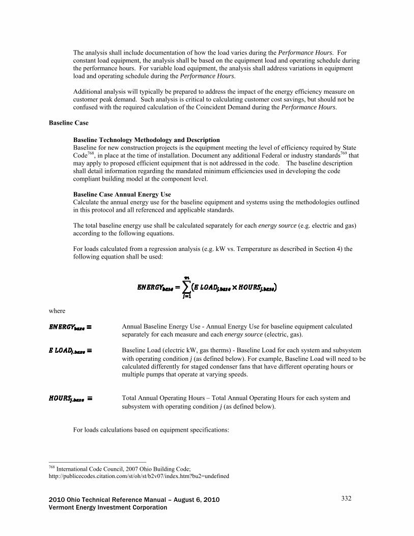
2010 Ohio Technical Reference Manual – August 6, 2010 332 Vermont Energy Investment Corporation
The analysis shall include documentation of how the load varies during the Performance Hours. For constant load equipment, the analysis shall be based on the equipment load and operating schedule during the performance hours. For variable load equipment, the analysis shall address variations in equipment load and operating schedule during the Performance Hours. Additional analysis will typically be prepared to address the impact of the energy efficiency measure on customer peak demand. Such analysis is critical to calculating customer cost savings, but should not be confused with the required calculation of the Coincident Demand during the Performance Hours.
Baseline Case
Baseline Technology Methodology and Description Baseline for new construction projects is the equipment meeting the level of efficiency required by State Code768, in place at the time of installation. Document any additional Federal or industry standards769 that may apply to proposed efficient equipment that is not addressed in the code. The baseline description shall detail information regarding the mandated minimum efficiencies used in developing the code compliant building model at the component level. Baseline Case Annual Energy Use Calculate the annual energy use for the baseline equipment and systems using the methodologies outlined in this protocol and all referenced and applicable standards. The total baseline energy use shall be calculated separately for each energy source (e.g. electric and gas) according to the following equations. For loads calculated from a regression analysis (e.g. kW vs. Temperature as described in Section 4) the following equation shall be used:
where
Annual Baseline Energy Use - Annual Energy Use for baseline equipment calculated separately for each measure and each energy source (electric, gas).
Baseline Load (electric kW, gas therms) - Baseline Load for each system and subsystem
with operating condition j (as defined below). For example, Baseline Load will need to be calculated differently for staged condenser fans that have different operating hours or multiple pumps that operate at varying speeds.
Total Annual Operating Hours – Total Annual Operating Hours for each system and
subsystem with operating condition j (as defined below). For loads calculations based on equipment specifications:
768 International Code Council, 2007 Ohio Building Code; http://publicecodes.citation.com/st/oh/st/b2v07/index.htm?bu2=undefined

2010 Ohio Technical Reference Manual – August 6, 2010 333 Vermont Energy Investment Corporation
where
Annual Baseline Energy Use - Annual Energy Use for baseline equipment calculated separately for each measure and each energy source (electric, gas).
Baseline Full Load - the maximum operating load of each baseline system and subsystem
with operating condition j (as defined below).
Load Factor - fraction of Full Load for each baseline system and subsystem with operating condition j (as defined below). Typically less than 1.00 unless the equipment was sized to run at 100% of rated capacity.
Total Annual Operating Hours – Total Annual Operating Hours for each system and
subsystem with operating condition j (as defined below).
System Condition - refers to each distinct combination of system mode, number of hours, Full Load demand, and Load Factor for each system or subsystem.
Number of Terms – total Number of Terms needed to cover all conditions of affected
systems and subsystems.
Document the inputs and outputs to the building model as described in the LEED Reference Guide for Green Building Design and Construction, Energy and Atmosphere Credit One, Option 1, Whole Building Simulation and as described in Section 4.
Baseline Case Coincident Electric Demand (kW) Document the baseline case coincident electric demand for each measure according to one of the following equations: For variable loads:
Where
Average Baseline Load of all affected equipment during the Performance Hours
of 3-6 pm, weekday, non-holidays from June 1 – August 31 for a total of 195 hours. Includes non-operating time during the Performance Hours and is equal to total energy use during the Performance Hours divided by the total Performance Hours.
For constant loads:
where
Average Coincident Baseline Load – average coincident load of all affected
baseline equipment during the Performance Hours of 3-6 pm, weekday, non-

2010 Ohio Technical Reference Manual – August 6, 2010 334 Vermont Energy Investment Corporation
holidays from June 1 – August 31 for a total of 195 hours. Includes non-operating time during the Performance Hours.
Baseline Full Load - the maximum nameplate load of each baseline system and
subsystem in operation during the Performance Hours with operating condition k (as defined below), exclusive of non operating time.
Load Factor - fraction of Full Load for each baseline system and subsystem with
operating condition k (as defined below). Typically less than 1.00 unless the equipment was sized to run at 100% of rated capacity.
Coincidence Factor - the Coincidence Factor is the fraction of time that each
baseline system and subsystem is operating during the Performance Hours for operating condition k (as defined below). The three typical conditions for CF are as follows: CF is unity if the equipment is continuously on during the Performance Hours; CF is zero for each system or subsystem that is not operating during the Performance Hours; otherwise, CF is the ratio of the ’on’ time to the total number of performance hours.
System Condition - refers to each distinct combination of the system mode (e.g.
high speed, low speed), Full Load demand, and Load Factor for each system or subsystem operating during Performance Hours.
Number of Terms – total Number of Terms needed to cover all operating modes
of affected systems and subsystems during Performance Hours. The analysis shall take into account that not all system components are expected to operate during all of the Performance Hours. For example on a cooling tower some of the cooling tower fans could periodically be staged in the “off” position while the compressors could be operating at 100% load. In these cases the system load during Performance Hours will not equal the sum of the loads for all system components. Document the modeled measure inputs and outputs specifically for the Performance Hours. The analysis shall include documentation of how the load varies during the Performance Hours. For constant load equipment, the analysis shall be based on the equipment load and operating schedule during the Performance Hours. For variable load equipment, the analysis shall address variations in equipment load and operating schedule during the Performance Hours. Additional analysis will typically be prepared to address the impact of the baseline equipment on customer peak demand. Such analysis is critical to calculating customer cost savings but should not be confused with the required calculation of the coincident demand during the Performance Hours.
Savings Savings shall be calculated from the efficient case and baseline case energy and demand calculations from above via whole building modeling. Ensure that the model addresses project variables as described in Section 3. Whole building models are designed to address interactive effects; the analyst shall ensure that the model accurately addresses such effects.
Annual Energy Savings (kWh for electrical, therms for gas)
where

2010 Ohio Technical Reference Manual – August 6, 2010 335 Vermont Energy Investment Corporation
and are defined above.
Coincident Electrical Demand Reduction (kW) =
where
and are defined above. Section 3: Project Variables Accurately capturing and documenting the variables that affect annual energy use and savings as well as those affecting peak period demand coincidence are critical elements in developing meaningful and reliable energy savings estimates. The savings analysis shall consider and address the variables over the life of the measure for both the baseline and efficient case. Uncertainty in variables shall be quantified and the savings analysis shall clearly demonstrate transparency and reasonableness in definition and application of variables affecting energy savings770. The variables below are common to many custom energy analyses. Document the variables that affect the energy use of the project for both the baseline and efficient scenarios. Describe the modeling methods used and any uncertainty associated with the values used in the model. ALL savings calculations must be normalized to reflect consistent application of the assumed variables for the project under both baseline and post-installation conditions over the full range of operating conditions for the affected systems. Modeling for new construction projects is the expected method for accounting for these variables as described in Section 4. Load Characterization Accurate characterization of the baseline and efficient energy use involves a comprehensive analysis of all variables that affect the loads over the analysis period. Concepts that are commonly used in performing energy analysis are discussed below. In all cases it is the intent of this document to require that the variations in load due to all factors (weather, production, schedule, etc) are accounted for in the analysis.
Load Shape The load shape reflects variations in load over the course of a year, with specific attention paid to the peak periods defined by the affected utility and/or regional transmission organization. The model shall generate an 8760 load shape771 that captures the expected period at which the load will operate at full load (full load hours) as well as all part load and non-operating or standby-modes..
Load Factor Load Factor is the ratio of maximum energy demand to the average electric demand for the affected end use. Analysis of loads across a representative sample of operating conditions can generate a single load factor for constant load applications. For variable load applications, a series of load factors must be developed to accurately represent the variations in energy use under the variety of loading conditions that occur over the range of operating cycles in a typical calendar year. Variable load analysis shall address the variations in load factor over a one year period for all dependent variables. Peak Load Factor Peak Load Factor describes the variation between the maximum connected load of the equipment and the highest actual load of the equipment. In some cases the Peak Load Factor is unity. For oversized
770 Anne Arquit Niederberger, PhD, A+B International (2005), Baseline Methodologies for Industrial End-Use Efficiency Presentation. Presented at World Bank; Anne_Arquit_Niederberger_Industry_EE_CDM_Dec_05.xls 771 Patil, Yogesh, et. al. (Aug, 2009) “Taking Engineering Savings to the Next Level, presented at IEPEC 2009 http://www.ers-inc.com/images/articles/Papers/takingsavingstonextlevel.pdf

2010 Ohio Technical Reference Manual – August 6, 2010 336 Vermont Energy Investment Corporation
equipment it is frequently less than one. In some rare instances where equipment is operated above its rated load, the Peak Load Factor may be greater than one.
Coincidence Factor Coincidence Factor is the coincidence of the demand savings during the Peak Performance Hours. For modeled measures, the average coincident demand, including non-operational hours, is generated through the hourly simulation of building demand for the baseline and efficient conditions during Peak Performance Hours.
Operating Conditions Characterize all variable operating conditions that affect the load over the analysis period. Typical operating variables are outlined below. Additional factors may be required to accurately characterize variability in equipment operations and the energy savings resulting from energy efficiency measures over the full range of operating conditions.
Operating Hours Establish the projected operating hours for all affected equipment in the building – scheduled operating hours are the same for base and efficient case models except where necessary to model nonstandard efficiency measures772. Address all variations in operating schedule over an annual operating cycle including, but not limited to weekends, holidays, and shift or occupancy changes that are a result in cyclical changes in operations over the course of a year. (For example retail applications may have longer operating hours in November and December). Project analysis shall clearly identify all operating, non-operating, and standby hours, the related loads, the periods for which those conditions apply and the basis for the assumptions in the analysis. Special attention should be paid that the hours of Coincident Peak (3:00 – 6:00 weekdays from June 1 through August 31) are detailed. Weather The analysis shall address the impact of annual weather, including temperature, humidity, and solar incidence (where applicable) on energy consumption. All savings (energy and demand) should be normalized to the TMY3 (Typical Meteorological Year) that corresponds to the nearest TMY3 weather site using modeling and/or regression analysis. TMY3 data should be obtained from National Renewable Energy Laboratory (NREL773) and used as the 8760 weather file to model and/or normalize annual energy use for weather dependent measures. Modeling tools, such as eQuest774, currently use TMY2 data. TMY3 data is based on more-recent and more accurate data and is available for many more locations; TMY3 data is available for over 1,000 locations, where TMY2 data is available for fewer than 300 locations. Production This applies only to industrial new construction projects that include production measures. Project analysis shall reflect variations in production over the cycles within the analysis period. Variations can include such things as the number of shifts or changes in quantity or type of product manufactured. For industrial process measures, production documentation shall normalize energy use based on the energy intensity of the process (i.e. energy use per unit of output) over the lifetime of the measure for both the baseline and efficient cases. Measurement of output should be based on physical measures of output (i.e. ton of steel or paper) and capture variations in both production levels and manufactured product types over the analysis period for both the baseline and efficient case775. Assumptions regarding economic climate, changes in production levels, and shifts all affect calculated energy savings over the life of the measures. Develop reasonable assumptions regarding these variables
772 ASHRAE Standard 90.1-2007 Energy Standard for Buildings Except Low-Rise Residential Buildings, Appendix G, Table G3.1, Section 4. 773 Typical Meteorological Data (TMY3) - http://rredc.nrel.gov/solar/old_data/nsrdb/1991-2005/tmy3/ 774 DOE2 eQuest simulation software - http://www.doe2.com/equest/ 9 Ruth, Michael, Lawrence Berkeley National Laboratory, et. al. (2001) A Process-Step Benchmarking Approach to Energy Use at Industrial Facilities: Examples from the Iron and Steel and Cement Industries; Process_Step_Benchmarking_ACEEE_LBNL-50444.doc

2010 Ohio Technical Reference Manual – August 6, 2010 337 Vermont Energy Investment Corporation
and ensure the application of these variables is clearly identified in both the analysis and project documentation. Identify the uncertainty introduced into the energy savings estimates as a result of these assumptions.
Controls Control settings and level of control shall be accounted for in the analysis in accordance with ASHRAE Standard 90.1 2007, Appendix G. Clearly document the control points that affect energy use, the control setpoints, sequence of operation and accuracy of controls that are required for the baseline case in Appendix G. Clearly document the changes in these conditions for the efficient case and how they are modeled. Include relevant information such as commissioning of control points, potential manual overrides of control sequences and anticipated control point calibration over the life of the measure. Occupancy Where occupancy affects energy use and varies over time, capture the variations in occupancy and their effects over the analysis period. At a minimum there is typically an ‘occupied’ and an ‘unoccupied’ mode for most facilities. Assumptions regarding economic climate and shifts in hours of occupancy affect calculated energy savings over the life of the measures. Develop reasonable assumptions regarding these variables and ensure the application of these variables is clearly identified in both the analysis and project documentation. Identify the uncertainty introduced into the energy savings estimates as a result of these assumptions.
Interactive Effects Analysis shall explicitly account for interactive effects between measures. For projects that include both prescriptive and custom measures, account for the energy use reduction from the prescriptive measure in the custom measure analysis. As prescriptive measures include interactive effects themselves, document the methodology that is used to ensure that savings from the interactive effects are only accounted for once in the claimed savings. One common set of interactive effects is the impact of electrical energy efficiency measures within a facility on that facility’s heating and/or cooling load. These shall be addressed as follows:
Waste Heat For efficiency upgrades that reduce the rejection of waste heat into air conditioned spaces (i.e. evaporator fans in a refrigerated enclosure), quantify the reduction in heat rejection776 and the associated cooling reduction.
Heating Increase For efficiency upgrades that reduce the rejection of waste heat into heated spaces, quantify the additional heating fuel required to offset the change and maintain temperature within the space14. The analysis shall address heating system efficiency and include basis for assumptions regarding fossil fuel increases.
For projects with multiple measures, the procedure for interactive effects is to calculate savings for the longest lived measure first, then consider that measure’s impact on the next longest-lived measure, and so on. This is because a short-lived measure can affect savings from a long-lived measure, but only for part of its life. Since tracking system limitations require that annual measure savings remain constant for all years, this is the only way to ensure proper lifetime savings and total resource benefits are captured.
Measure Life Document both the life of the baseline and efficient case equipment. The efficient case analysis is typically performed over the lifetime of the efficiency measures. Where the analysis period and the efficiency measure life are not the same, describe the rationale for the analysis period and assumptions regarding replacement equipment for measures with lives that are shorter than the analysis period.
776 2009 ASHRAE Handbook, Fundamentals, Chapter 18, page 18.3.

2010 Ohio Technical Reference Manual – August 6, 2010 338 Vermont Energy Investment Corporation
Persistence Persistence factors may be used to reduce lifetime measure savings in recognition that initial engineering estimates of annual savings may not persist long term777. The persistence factor accounts for uncertainties and for normal operations over the life of the measure. For instance if energy efficient motors are installed as part of a process and the customer’s standard procedure is to have motors rewound upon failure, the energy efficiency associated with the efficient motor would only persist until the expected time when the motor is rewound. Persistence is also affected by measures being removed or failing prior to the end of its normal engineering lifetime, improper maintained over the life of the measure, control overrides or loss of calibration (controls only), etc. Related Variables: Related variables are those which are not included in the energy and demand calculations, but may be required for project cost-effectiveness screening by the utility(ies). Document the following variables for the project:
Operation &Maintenance (O&M) Impacts Where O&M practices would have resulted in changes to the baseline during the analysis period, account for such practices in the establishment of baseline and efficiency case energy use.
Water Consumption Impacts Quantify any changes in water consumption attributable to the project.
Cost Document the cost of each measure. Include invoices, bids and other documentation to substantiate project cost data. Identify portions of the cost which are for equipment being purchased for redundancy or backup and will not generate savings in the project. Related costs such as the costs for audits, design, engineering, permits, fees or M&V should be reported separately from the costs associated with the design and installation of energy efficiency improvements.
Other Variables As needed - clearly document all variables affecting the energy use of the project that have not been covered in this document. Section 4: Documentation and Modeling Documentation and modeling of custom new construction projects are essential to developing reliable energy savings and peak demand reductions claims.778 The following guidelines support the accurate estimation of energy and demand savings. Modeling Computer modeling is an acceptable method of analysis using an 8760 model which meets the requirements of ASHRAE 90.1 Appendix G and the requirements of the LEED Reference Guide for Green Building Design and Construction, Energy and Atmosphere Credit One, Option 1, Whole Building Simulation. Process measures, such as industrial process or data center efficiency that are additional to the building design modeled under ASHRAE 90.1 Appendix G shall be either included in the simulation using customized algorithms, or modeled separately using measure specific analysis tools. The results of measure specific analysis shall be accounted for in the building model and any custom simulations should be documented in accordance with the TRM and the Custom Analysis Template (Appendix B). Calculations Computer simulation of energy efficiency measures using 8760 hourly simulation models such as eQuest, or customized spreadsheet analysis or other energy analysis tools shall be employed to calculate energy savings. The
777 Efficiency Vermont Technical Reference User Manual (TRM) Measure Savings Algorithms and Cost Assumptions, February 19, 2010 778 Parlin, Kathryn, et. al. (August, 2009 IEPEC) “Demand Reduction in the Forward Capacity Market, Verifying the Efficiency Power Plant”

2010 Ohio Technical Reference Manual – August 6, 2010 339 Vermont Energy Investment Corporation
algorithms of the modeling software must be designed to address the modeled measures. Minimum documentation requirements include model output reports stating unmet load hours for the baseline and efficient case, hourly energy use and demand, and electronic copies of the model or spreadsheet analysis files.
Annual kWh and therms for baseline and efficient cases shall be the annualized and normalized per the equations in Section 2 using the methods described above. Document the assumptions and calculations for baseline and efficient Coincident Electric Demand (kW) as the average kW over the Performance Hours as indicated in Section 2. Calculation documentation shall include definitions and reference sources for all variables and assumed factors in Section 3.
Documentation Analysis shall be documented with comprehensive, well labeled supporting information including, but not limited to:
Manufacturer literature documenting connected load for both the baseline and the installed equipment or manufacturer data documenting the information necessary to calculate peak demand (such as horsepower, voltage, efficiency, etc.) shall be included in the project documentation. Manufacturer data shall be clearly marked to indicate the specific equipment model number and data that is applicable to the project and used in the calculations.
Reporting The following shall be reported:
All information required in this protocol Custom Analysis Template (Appendix B) Section 1 and Documentation Worksheet (Appendix C) only Documentation as required by LEED Reference Guide for Green Building Design and Construction,
Energy and Atmosphere Credit One, Option 1, Whole Building Simulation. Assessment of the level of uncertainty associated with the energy and demand calculated savings. Project commissioning can reduce energy use and is recommended. If the project was commissioned,
submit a copy of the commissioning report.
2010 Ohio Technical Reference Manual – August 6, 2010 340 Vermont Energy Investment Corporation
V. Protocols for Transmission & Distribution Projects
T&D Loss Reductions – Mass Plant Replacement and Expansion Analysis Protocol This protocol defines the requirements for analyzing and documenting loss reductions due to installation of mass utility plant with lower losses than standard equipment, when that equipment is required due to failure, need for increased capacity, or connection of new loads. Where equipment is replaced prior to the end of its rated service life in order to achieve energy savings, the project is classified as Retrofit and the “T&D Loss Reductions – Mass Plant Retrofit Analysis Protocol” should be used to guide analysis. Examples of mass plant include line transformers, secondary lines, service drops, and meters. For these common and generally small investments, determination of loads and losses for each installation will not generally be feasible or cost-effective. This protocol is intended to address the energy impacts of operating energy efficiency improvements of installed equipment on average over many installations. This analysis protocol does not apply to equipment installed to serve interval-metered load in excess of 500 kVA. Those projects should be analyzed with the Large Customer Connection Analysis Protocol. The Analysis Protocol is divided into four sections: Section 1: Program Information Section 2: Equipment Loading Section 3: Base and Efficient Cases and Savings Section 4: Screening Inputs Section 1: Program Information Program Title Provide a unique title for the program so that it is easily distinguishable from other programs with similar scope. Example: “50 kVA 13.8 kV transformers specified for new connections”. Sites (locations) Provide a list of the locations at which equipment was installed under this program. Locations may be identified by the customer addresses, pole numbers, transformer identification numbers, or similar identifiers. Class/Sector/Industry Description For each installation, specify the customer classes (residential, small general service, etc.) served by the equipment, and for non-residential customers, the sector (Industrial, Commercial, Institutional, Multi-family) and type of use (e.g., office, restaurant, dormitory, gas station). Technology Description Describe the type of equipment affected (e.g., line transformer, secondary, etc.), including the range of capacities, wire sizes, span lengths, or other descriptors affecting energy losses. Describe the base-efficiency equipment that would be installed under current standard utility practice. Describe the high-efficiency equipment installed in the program. Provide specific details (e.g., wire sizes, transformer loss specifications) relevant to loss computations. Program Implementation schedule Define the implementation schedule for the program, including number of installations by month. Analysis Contact(s)

2010 Ohio Technical Reference Manual – August 6, 2010 341 Vermont Energy Investment Corporation
Provide contact information for the personnel responsible for tracking installations and for estimating loss reductions, including company name, individual(s) name, address, phone and email. Section 2: Equipment Loading For each type of equipment included in the program, provide (1) the estimated maximum load on the typical or average installation, (2) the estimated average load on the equipment on weekdays between 3:00 p.m. and 6:00 p.m., June through August (the coincident peak period), and (3) the estimated load-duration curve on the equipment.
Include the sources of the estimates, including utility load-research data. Include any data on the variability of loads among installations, reflecting the number of customers served by the equipment (e.g., customers on a transformer or a span of secondary), the size of customer, and the customer class(es) (e.g., residential, street lighting, small commercial) served.
The load data should reflect the conditions prevailing in the year for which savings are claimed. Particularly for expansions of the distribution system, the loads in the year of installation may be less than loads in later years. Where possible, the annual billed sales to the customers served by the equipment should be used as a check on the total energy usage assumed. Where these data are not available, describe the system configuration (e.g., secondary network) or database limitations that prevent such comparison. Section 3: Base and Efficient Cases Calculate and document energy losses for the efficient and base cases as outlined below. Baseline-Case Losses For each type of equipment included in the program, compute the annual losses per unit of equipment as
lossbase = Σt [kVAt ÷ FLC]2 × FLLLb + 8766 × NLLb
where t = hour FLC = full-load capacity FLLLb = load losses at full load NLLb = no-load loss/hour
Compute the pre-project losses in the coincident peak period in kW as
peaklossbase = Σh {[kVAh ÷ FLC]2 × FLLLb} ÷ H + NLLb
where h = hour in the coincident peak period H = number of hours in the coincident peak period
Provide manufacturer’s specifications or standard-reference data for typical baseline equipment for FLC, FLLL, and NLL. Provide the spreadsheet in which the base losses are computed. Provide information demonstrating that the assumed base efficiency is in fact standard practice, including:
Current Industry Practice – Document current industry practice using articles from industry journals, manufacturers’ sales data, recent distribution standards from other utilities, and/or similar sources.

2010 Ohio Technical Reference Manual – August 6, 2010 342 Vermont Energy Investment Corporation
Applicant Practice – Document the utility’s own recent standard practices through purchase records, distribution standards, internal guidelines for linemen, and similar documents. Document the effect on equipment selection of allowances for growth, including new infill construction in expansion applications.
Efficient-Case Losses For each type of equipment included in the program, compute the annual losses per unit of the efficient equipment as
lossefficient = Σt [kVAt ÷ FLC]2 × FLLLe + 8766 × NLLe
where t = hour FLC = full-load capacity FLLLe = load losses at full load NLLe = no-load loss/hour
Compute the post-project losses in the coincident peak period in kW as
peaklossefficient = Σh {[kVAh ÷ FLC]2 × FLLLe} ÷ H + NLLe
where h = hour in the coincident peak period H = number of hours in the coincident peak period
Provide manufacturer’s specifications or standard-reference data for efficient equipment for FLC, FLLL, and NLL. Provide the spreadsheet in which the efficient-case losses are computed. Savings
Energy Savings = (lossbase – lossefficient) × (1 + ULF) where ULF = Upstream Loss Factor, the change in losses on the primary distribution and
transmission systems per kWh reduction in secondary losses Peak Savings = (peaklossbase – peaklossefficient) × (1 + UPLF) where ULF = Upstream Peak Loss Factor applicable to the coincident peak period
If the utility has estimates of load-related losses on the primary distribution and transmission systems, and uses those estimates in screening customer end-use efficiency measures, it may add those losses to the load reduction due to efficiency improvements in mass plant on the secondary distribution system. Provide the derivation of the estimate of primary and transmission losses, and demonstrate the consistency of the claimed losses with the loss values used for the savings behind the customer meter. Section 4: Screening Inputs Measure Life Document the life of each type of added equipment, including reference to the utility’s depreciation studies. The efficient case analysis is typically performed over the lifetime of the major components. Where some equipment has a useful life shorter than the analysis period, describe the rationale for the analysis period and assumptions regarding the replacement cost of equipment with lives shorter than the analysis period.

2010 Ohio Technical Reference Manual – August 6, 2010 343 Vermont Energy Investment Corporation
Discount savings with respect to existing equipment over time, to the extent that the utility would make this (or a similar) change in configuration in the foreseeable future to meet peak load or reliability requirements. O&M Cost Effects Include any foreseeable changes in O&M costs related to the changes in equipment and to any changes in operating practices. Cost Document the actual cost of the project, including equipment, internal and contract labor, allocated overheads, design, engineering, and permitting.

2010 Ohio Technical Reference Manual – August 6, 2010 344 Vermont Energy Investment Corporation
T&D Loss Reductions – Mass Plant Retrofit Analysis Protocol This protocol defines the requirements for analyzing and documenting loss reductions due to replacement of existing mass utility plant with more efficient equipment, prior to the end of the existing equipment’s useful life and in the absence of any need for increased capacity. Examples of mass plant include line transformers, secondary lines, service drops and meters. For these common and generally small investments, determination of loads and losses for each installation will not generally be feasible or cost-effective. This protocol is intended to address the energy impacts of operating energy efficiency improvements of installed equipment on average over many installations. This analysis protocol does not apply to equipment installed to serve interval-metered load in excess of 500 kVA. Those projects should be analyzed with the Large Customer Analysis Protocol. The Analysis Protocol is divided into four sections: Section 1: Program Information Section 2: Equipment Loading Section 3: Base and Efficient Cases and Savings Section 4: Screening Inputs Section 1: Program Information Program Title Provide a unique title for the program so that it is easily distinguishable from other programs with similar scope. Example: “Replacing 25 kVA 13.8 kV transformers with amorphous-core transformers”. Sites (locations) Provide a list of the locations at which equipment was installed under this program. Locations may be identified by the customer addresses, pole numbers, transformer identification numbers, or similar identifiers. Class/Sector/Industry Description For each installation, specify the customer classes (residential, small general service, etc.) served by the equipment, and for non-residential customers, the sector (Industrial, Commercial, Institutional, Multi-family) and type of use (e.g., office, restaurant, dormitory, gas station). Technology Description Describe the type of equipment affected (e.g., line transformer, secondary, etc.), including the range of capacities, wire sizes, span lengths, or other descriptors affecting energy losses. Describe the existing equipment that was replaced. Describe the high-efficiency equipment installed in the program. Provide specific details (e.g., wire sizes, transformer loss specifications) relevant to loss computations. Program Implementation schedule Define the implementation schedule for the program, including number of installations by month. Analysis Contact(s) Provide contact information for the personnel responsible for tracking installations and for estimating loss reductions, including company name, individual(s) name, address, phone and email. Section 2: Equipment Loading
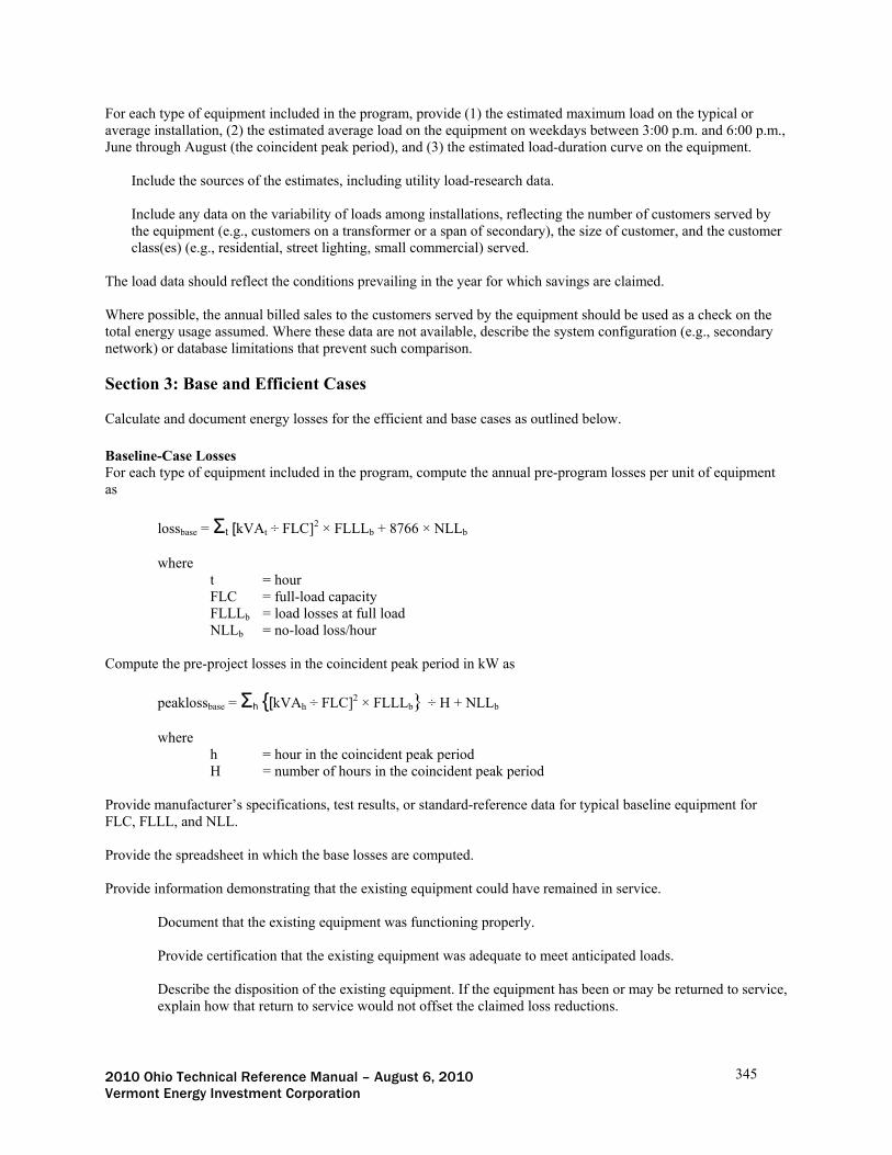
2010 Ohio Technical Reference Manual – August 6, 2010 345 Vermont Energy Investment Corporation
For each type of equipment included in the program, provide (1) the estimated maximum load on the typical or average installation, (2) the estimated average load on the equipment on weekdays between 3:00 p.m. and 6:00 p.m., June through August (the coincident peak period), and (3) the estimated load-duration curve on the equipment.
Include the sources of the estimates, including utility load-research data. Include any data on the variability of loads among installations, reflecting the number of customers served by the equipment (e.g., customers on a transformer or a span of secondary), the size of customer, and the customer class(es) (e.g., residential, street lighting, small commercial) served.
The load data should reflect the conditions prevailing in the year for which savings are claimed. Where possible, the annual billed sales to the customers served by the equipment should be used as a check on the total energy usage assumed. Where these data are not available, describe the system configuration (e.g., secondary network) or database limitations that prevent such comparison. Section 3: Base and Efficient Cases Calculate and document energy losses for the efficient and base cases as outlined below. Baseline-Case Losses For each type of equipment included in the program, compute the annual pre-program losses per unit of equipment as
lossbase = Σt [kVAt ÷ FLC]2 × FLLLb + 8766 × NLLb
where t = hour FLC = full-load capacity FLLLb = load losses at full load NLLb = no-load loss/hour
Compute the pre-project losses in the coincident peak period in kW as
peaklossbase = Σh {[kVAh ÷ FLC]2 × FLLLb} ÷ H + NLLb
where h = hour in the coincident peak period H = number of hours in the coincident peak period
Provide manufacturer’s specifications, test results, or standard-reference data for typical baseline equipment for FLC, FLLL, and NLL. Provide the spreadsheet in which the base losses are computed. Provide information demonstrating that the existing equipment could have remained in service.
Document that the existing equipment was functioning properly. Provide certification that the existing equipment was adequate to meet anticipated loads. Describe the disposition of the existing equipment. If the equipment has been or may be returned to service, explain how that return to service would not offset the claimed loss reductions.

2010 Ohio Technical Reference Manual – August 6, 2010 346 Vermont Energy Investment Corporation
Describe the manner in which equipment was selected for replacement (e.g., vintage, design, location), and provide documentation to demonstrate that the replacements were targeted for loss reduction, rather than actual or imminent failure.
Efficient-Case Losses For each type of equipment included in the program, compute the annual losses per unit of the efficient equipment as
lossefficient = Σt [kVAt ÷ FLC]2 × FLLLe + 8766 × NLLe
where t = hour FLC = full-load capacity FLLLe = load losses at full load NLLe = no-load loss/hour
Compute the post-project losses in the coincident peak period in kW as
peaklossefficient = Σh {[kVAh ÷ FLC]2 × FLLLe} ÷ H + NLLe
where h = hour in the coincident peak period H = number of hours in the coincident peak period
Provide manufacturer’s specifications or standard-reference data for efficient equipment for FLC, FLLL, and NLL. Provide the spreadsheet in which the efficient-case losses are computed. Savings
Energy Savings = (lossbase – lossefficient) × (1 + ULF) where ULF = Upstream Loss Factor, the change in losses on the primary distribution and
transmission systems per kWh reduction in secondary losses Peak Savings = (peaklossbase – peaklossefficient) × (1 + UPLF) where ULF = Upstream Peak Loss Factor applicable to the coincident peak period
If the utility has estimates of load-related losses on the primary distribution and transmission systems, and uses those estimates in screening customer end-use efficiency measures, it may add those losses to the load reduction due to efficiency improvements in mass plant on the secondary distribution system. Provide the derivation of the estimate of primary and transmission losses, and demonstrate the consistency of the claimed losses with the loss values used for the savings behind the customer meter. Section 4: Screening Inputs Measure Life Document the life of each type of added equipment, including reference to the utility’s depreciation studies. The efficient case analysis is typically performed over the lifetime of the major components. Where some equipment has a useful life shorter than the analysis period, describe the rationale for the analysis period and assumptions regarding the replacement cost of equipment with lives shorter than the analysis period.

2010 Ohio Technical Reference Manual – August 6, 2010 347 Vermont Energy Investment Corporation
Discount savings with respect to existing equipment over time, to the extent that the utility would make this (or a similar) change in configuration in the foreseeable future to meet peak load or reliability requirements. O&M Cost Effects Include any foreseeable changes in O&M costs related to the changes in equipment and to any changes in operating practices. Cost Document the actual cost of the project, including equipment, internal and contract labor, allocated overheads, design, engineering, and permitting.

2010 Ohio Technical Reference Manual – August 6, 2010 348 Vermont Energy Investment Corporation
T&D Loss Reductions – Large Customer Connection Analysis Protocol This protocol defines the requirements for analyzing and documenting loss reductions due to installation of distribution equipment to serve interval-metered load in excess of 500 kVA, where the installed equipment has lower losses than standard equipment, in the case of incremental improvements over equipment required due to failure, need for
increased capacity, or connection of new loads, or existing equipment, in the case of retrofit of equipment solely for the energy savings. Each project may include equipment serving one or a few customers, each with interval metering, at single location. The equipment may also serve small amounts of non-interval-metered street lighting and private area lighting, so long as the load shape of the outdoor lighting can be reasonably estimated. Examples of distribution plant covered by this protocol include line transformers, secondary lines, service drops, and meters. The Analysis Protocol is divided into four sections: Section 1: Project Information Section 2: Equipment Loading Section 3: Base and Efficient Cases and Savings Section 4: Screening Inputs Section 1: Project Information Project Title Provide a unique title for the project so that it is easily distinguishable from other projects with similar scope. Example: “Install low-loss transformers and upgrade service drops for the Midway Office Park”. Sites (locations) Provide a list of the locations at which equipment was installed under this project. Locations may be identified by the customer number, address, pole numbers, transformer identification numbers, or similar identifiers. Technology Description Describe the type of equipment affected (e.g., line transformer, secondary, etc.), including the capacity, wire size, span lengths, voltages, or other descriptors affecting energy losses. Provide a one-line diagram of the interconnection. If this project consists of the incremental increase of efficiency for a new or replacement connection, describe the equipment that would be installed under standard utility practice. Demonstrate that the assumed base efficiency is in fact standard practice, including:
Current Industry Practice – Document current industry practice using articles from industry journals, manufacturers’ sales data, recent distribution standards from other utilities, and/or similar sources.
Applicant Practice – Document the utility’s own recent standard practices through purchase records, distribution standards, internal guidelines for linemen, and similar documents. Document the effect on equipment selection of allowances for growth, including new infill construction in expansion applications.
If this project consists of the loss-driven retrofit of existing connection equipment, describe the existing equipment. Describe the high-efficiency equipment installed in the project. Provide specific details (e.g., wire sizes, transformer loss specifications) relevant to loss computations.

2010 Ohio Technical Reference Manual – August 6, 2010 349 Vermont Energy Investment Corporation
Project Implementation schedule Describe the implementation schedule for the project. Analysis Contact(s) Provide contact information for the personnel responsible for tracking installations and for estimating loss reductions, including company name, individual(s) name, address, phone and email. Section 2: Equipment Loading Provide the hourly customer loads at this location in the report year. If individual loads use only some of the equipment contributing to the efficiency improvement, disaggregate the loads so that load can be determined for each piece of equipment. Determine
(1) the average load on the line at its input on weekdays between 3:00 p.m. and 6:00 p.m., June through August (2) total energy delivered to the line.
Where possible, the annual billed sales to the customers served by the equipment should be used as a check on the total energy usage assumed. Where these data are not available, describe the system configuration (e.g., secondary network) or database limitations that prevent such comparison. Section 3: Base and Efficient Cases Calculate and document energy losses for the efficient and base cases as outlined below. Baseline-Case Losses Compute the annual base losses in kWh as
lossbase = Σt [kVAt ÷ FLC]2 × FLLLb + 8766 × NLLb
where t = hour FLC = full-load capacity or other convenient reference load FLLLb = load losses at FLC NLLb = no-load loss per hour
Compute the pre-project losses in the coincident peak period in kW as
peaklossbase = Σh {[kVAh ÷ FLC]2 × FLLLb} ÷ H + NLLb
where h = hour in the coincident peak period H = number of hours in the coincident peak period
Where various pieces of equipment are subject to different loadings (e.g., the transformer bank serves the entire load, while each section of secondary serves half the load), compute losses for each type of equipment or load grouping. Provide manufacturer’s specifications or standard-reference data for typical baseline equipment for FLC, FLLL, and NLL.

2010 Ohio Technical Reference Manual – August 6, 2010 350 Vermont Energy Investment Corporation
Provide the spreadsheet in which the base losses are computed. Efficient-Case Losses Compute the annual losses of the efficient equipment as
lossefficient = Σt [kVAt ÷ FLC]2 × FLLLe + 8766 × NLLe
where t = hour FLC = full-load capacity FLLLe = load losses at full load NLLe = no-load loss per hour
Compute the post-project losses in the coincident peak period in kW as
peaklossefficient = Σh {[kVAh ÷ FLC]2 × FLLLe} ÷ H + NLLe
where h = hour in the coincident peak period H = number of hours in the coincident peak period
Provide manufacturer’s specifications or standard-reference data for typical baseline equipment for FLC, FLLL, and NLL. Provide the spreadsheet in which the efficient-case losses are computed. Savings
Energy Savings = (lossbase – lossefficient) × (1 + UELF) where ULEF = Upstream Energy Loss Factor, the annual average change in losses on the primary
distribution and transmission systems per kWh reduction in secondary losses Peak Savings = (peaklossbase – peaklossefficient) × (1 + UPLF) where UPLF = Upstream Peak Loss Factor, the change in losses on the primary distribution and
transmission systems per kWh reduction in secondary losses in the coincident peak period
If the utility has estimates of load-related losses on the primary distribution and transmission systems, and uses those estimates in screening customer end-use efficiency measures, it may add those losses to the load reduction due to efficiency improvements on the secondary distribution system. Provide the derivation of the estimate of primary and transmission losses, and demonstrate the consistency of the claimed losses with the loss values used for the savings behind the customer meter. Section 4: Screening Inputs Measure Life Document the life of each type of added equipment, including reference to the utility’s depreciation studies. The efficient case analysis is typically performed over the lifetime of the major components. Where some equipment has a useful life shorter than the analysis period, describe the rationale for the analysis period and assumptions regarding the replacement cost of equipment with lives shorter than the analysis period.

2010 Ohio Technical Reference Manual – August 6, 2010 351 Vermont Energy Investment Corporation
Discount savings with respect to existing equipment over time, to the extent that the utility would make this (or a similar) change in configuration in the foreseeable future to meet peak load or reliability requirements. O&M Cost Effects Include any foreseeable changes in O&M costs related to the changes in equipment and to any changes in operating practices. Cost Document the actual cost of the project, including equipment, internal and contract labor, allocated overheads, design, engineering, and permitting.
2010 Ohio Technical Reference Manual – August 6, 2010 352 Vermont Energy Investment Corporation
T&D Loss Reductions – Substation Transformer Analysis Protocol This protocol defines the requirements for analyzing and documenting loss reductions due to installation of efficient substation transformers in any of the following contexts: Incremental: installation of one or more high-efficiency transformers instead of a new standard-efficiency
transformer when a new transformer is required at a new substation, to increase capacity at an existing substation, to replace a failed or failing transformer
Retrofit: replacement of an existing transformer with a more efficient transformer, which may be more efficient due to higher-efficiency materials (such as an amorphous core) or due to lower capacity (with lower core losses).
Addition of a transformer or substation to change power flow on the network should be analyzed with the System Reconfiguration Protocol. The Analysis Protocol is divided into four sections: Section 1: Project Information Section 2: Equipment Loading Section 3: Base and Efficient Cases and Savings Section 4: Screening Inputs Section 1: Project Information Project Title Provide a unique title for the project. Example: “Installation of low-loss amorphous-core transformers at the Midway 138-12.5 kV substation”. Location Identify the location of the project, by substation name, number, and address. Technology Description Describe the transformer(s) affected, including voltages and capacity. Describe the high-efficiency transformer(s) installed in the project. Provide manufacturer specifications. If this project consists of the incremental increase of efficiency at a new transformer, describe the standard-efficiency transformer that would have been installed under standard utility practice. If this project consists of the retrofit of a lower-loss transformer in place of an existing transformer, describe the existing equipment that was replaced. Project Implementation schedule Define the implementation schedule for the project, including the date at which the transformer(s) were energized by month. Analysis Contact(s) Provide contact information for the personnel responsible for tracking installations and for estimating loss reductions, including company name, individual(s) name, address, phone and email.
Section 2: Equipment Loading

2010 Ohio Technical Reference Manual – August 6, 2010 353 Vermont Energy Investment Corporation
Provide the hourly load the transformer or substation in the current year and identify:
(1) the maximum load on the equipment (2) the average load on the equipment on weekdays between 3:00 p.m. and 6:00 p.m., June through August (the coincident peak period)
Section 3: Base and Efficient Cases Calculate and document energy losses for the efficient and base cases as outlined below. Baseline-Case Losses For each transformer included in the project, compute the annual pre-project losses in kWh as
lossbase = Σt [kVAt ÷ FLC]2 × FLLLb + 8766 × NLLb
where t = hour FLC = full-load capacity FLLLb = load losses at full load NLLb = no-load loss/hour
Compute the pre-project losses in the coincident peak period in kW as
peaklossbase = Σh {[kVAh ÷ FLC]2 × FLLLb} ÷ H + NLLb
where h = hour in the coincident peak period H = number of hours in the coincident peak period
Provide manufacturer’s specifications, test results, or standard-reference data for the baseline transformer for FLC, FLLL, and NLL. Provide the spreadsheet in which the base losses are computed. If this project consists of the incremental increase of efficiency at a new transformer, provide information demonstrating that the assumed base efficiency is in fact standard practice, including:
Current Industry Practice – Document current industry practice using articles from industry journals, manufacturers’ sales data, recent distribution standards from other utilities, and/or similar sources.
Applicant Practice – Document the utility’s own recent standard practices through purchase records, distribution standards, and similar documents. Provide data on peak forecasts for the substation, supporting the adequacy of the base equipment.
If this project consists of the retrofit of a lower-loss transformer in place of an existing transformer,
Describe the existing equipment that was replaced.
Provide information demonstrating that the existing equipment could have remained in service. Document that the existing equipment was functioning properly.

2010 Ohio Technical Reference Manual – August 6, 2010 354 Vermont Energy Investment Corporation
Provide certification that the existing equipment was adequate to meet anticipated loads. Describe the disposition of the existing equipment. If the equipment has been or may be returned to service, explain how that return to service would not offset the claimed loss reductions. Describe the manner in which the equipment was selected for replacement, and provide documentation to demonstrate that the retrofit was undertaken for loss reduction, rather than actual or imminent failure or inadequacy.
Efficient-Case Losses For each transformer included in the project, compute the annual post-project losses in kWh as
lossefficient = Σt [kVAt ÷ FLC]2 × FLLLe + 8766 × NLLe
where t = hour FLC = full-load capacity FLLLe = load losses at full load NLLe = no-load loss/hour
Compute the post-project losses in the coincident peak period in kW as
peaklossefficient = Σh {[kVAh ÷ FLC]2 × FLLLe} ÷ H + NLLe
where h = hour in the coincident peak period H = number of hours in the coincident peak period
Provide manufacturer’s specifications the installed transformer for FLC, FLLL, and NLL. Provide the spreadsheet in which the efficient-case losses are computed. Savings
Energy Savings = (lossbase – lossefficient) × (1 + TELF) where TELF = Transmission Energy Loss Factor applicable to the transmission system upstream from
the project substation Peak Savings = (peaklossbase – peaklossefficient) × (1 + TPLF) where TPLF = Transmission Peak Loss Factor applicable to the transmission system upstream from
the project substation
If the utility has estimates of load-related losses on the transmission system, and uses those estimates in screening customer end-use efficiency measures, it may add those losses to the load reduction due to efficiency improvements at distribution substations. For transmission substations, the utility may compute TLF as the portion of transmission losses attributable to voltages equal to or higher than those of the input voltage to the transformer. Provide the derivation of the estimate of transmission losses, and demonstrate the consistency of the claimed losses with the loss values used for the savings behind the customer meter. Section 4: Screening Inputs

2010 Ohio Technical Reference Manual – August 6, 2010 355 Vermont Energy Investment Corporation
Measure Life Document the life of each type of added equipment, including reference to the utility’s depreciation studies. The efficient case analysis is typically performed over the lifetime of the major components, in this case the transformers. Where some equipment has a useful life shorter than the analysis period, describe the assumptions regarding the replacement cost of equipment with lives shorter than the analysis period. Where the utility would make a similar investment in the foreseeable future to meet peak load or reliability requirements, the analysis period should be limited to the period prior to that need date, and reflect the present value of the differences in capital costs. Operations Effects The estimates of baseline and efficiency case losses should reflect the operating practices expected to be in place for the base and efficient equipment. O&M Cost Effects Include any foreseeable changes in O&M costs related to the change in equipment (including the effect of replacing old equipment with new equipment) and to any changes in operating practices. Cost Document the actual cost of the project, including equipment, internal and contract labor, allocated overheads, design, engineering, and permitting.

2010 Ohio Technical Reference Manual – August 6, 2010 356 Vermont Energy Investment Corporation
T&D Loss Reductions – System Reconfiguration Analysis Protocol This protocol defines the requirements for analyzing and documenting loss reductions due to changes undertaken to change network power flows and reduce losses, including (but not necessarily limited to) any of the following contexts: Addition of a substation or substation transformer. Addition of a new primary circuit or transmission line. Addition of capacitors. The Analysis Protocol is divided into four sections: Section 1: Project Information Section 2: Equipment Loading Section 3: Base and Efficient Cases and Savings Section 4: Screening Inputs Section 1: Project Information Project Title Provide a unique title for the project. Example: “Installation of new Midway 138-12.5 kV substation and reconfiguration of feeders K181 and K182”. Location Identify the location of the project, by substation name, number, and address; line number and connecting substations; and/or other relevant identification. Technology Description Describe the equipment added, including voltages and capacity, and the major network elements (lines and substations) affected by the reconfiguration. If the project includes the addition of capacitors, describe the connection of the capacitors (e.g., shunt, series), their kVAR capacity, and the levels to which they can be switched. Project Implementation schedule Define the implementation schedule for the project, including the date at which each major project element was put into service. Analysis Contact(s) Provide contact information for the personnel responsible for tracking installations and for estimating loss reductions, including company name, individual(s) name, address, phone and email. Section 2: Equipment Loading Provide the hourly loads on each of the major affected network elements for the last full year prior to the installation of the first element of the project. For the current year, provide the hourly loads on
(1) each of the major affected network elements identified above
(2) each major element of the project (e.g., line, transformer or substation) in. For capacitors, provide

2010 Ohio Technical Reference Manual – August 6, 2010 357 Vermont Energy Investment Corporation
(1) the hourly loads in the current year on the substation or other equipment to which the capacitors are
attached. (2) the hours in the current year for which the capacitors were activated at each kVAR level
Based upon the loading of the new equipment, identify N load patterns, such that each hour within the year is reasonably well represented by a load pattern and N is a tractable number for modeling and evaluation.
At least one load pattern should represent typical power flows during the coincident peak period (weekdays between 3:00 p.m. and 6:00 p.m., June through August).
The load pattern should be representative of the hours modeled, in terms of the direction of power flow, the level of power flow, and the operation of capacitors.
Describe the load-pattern selection process. Identify the hours that are represented by each load pattern. Loss reductions in some hours may be zero or nearly so (e.g., hours in which capacitors are switched off, hours with very low flows on the affected equipment). These hours may be ignored, so long as any increase in no-load losses is also insignificant.
Section 3: Base and Efficient Cases Calculate and document energy losses for the efficient and base cases as outlined below. Baseline-Case Losses Using computer software appropriate to the application, model the relevant portions of the distribution and/or transmission system for each load pattern n (where n = 1 to N). Compute lossn, the sum of load and no-load losses in the study area for load pattern n. Where possible, compare the transmission flows and losses modeled for the load pattern for the actual metered loads in some hours of the pre-project historical period. Where such comparisons are not possible, explain why. Determine annualized base pre-project losses in kWh as
lossbase = Σn lossn,b × hoursn (1) where n = load pattern, n = 1 to N lossn,b = total modeled base losses in the study area hoursn = hours in load pattern n
Compute the pre-project losses in the coincident peak period in kW as
peaklossbase = Σn lossn,b × hoursn ÷ H (2) where n = load pattern, for those load patterns representing the coincident peak period H = number of hours in the coincident peak period
Provide the spreadsheet in which the base losses are computed.

2010 Ohio Technical Reference Manual – August 6, 2010 358 Vermont Energy Investment Corporation
Post-project Losses Using actual metered data where available and modeling results otherwise (using the same software used in the base case), compute total load and no-load losses in the study area for each load pattern for the actual conditions in the report year, with the project. Compute annual post-project losses as
lossefficient = Σn lossm,n,e × hoursn + Σt lossa,t (3)
where lossm,n,e = losses in modeled load pattern n with the post-project actual configuration t = hours in the year, excluded hours expected to have negligible loss reductions lossa,t = actual losses in hour t in the report year
Compute the pre-project losses in the coincident peak period in kW as
peaklossbase = Σn {lossn,e × hoursn + Σh lossa,h }÷ H (4)
where n = load pattern, for those load patterns representing the coincident peak period h = hour in the coincident peak period in the report year H = number of hours in the coincident peak period
For comparison, provide the total modeled losses for the year and in the coincident peak period, with the post-project configuration. Savings
Energy Savings = (lossbase – lossefficient) × (1 + TELF) where TELF = Transmission Energy Loss Factor applicable to the transmission system upstream from
the study area Peak Savings = (peaklossbase – peaklossefficient) × (1 + TPLF) where TPLF = Transmission Peak Loss Factor applicable to the transmission system upstream from
the study area
If the utility has estimates of load-related losses on the transmission system, and uses those estimates in screening customer end-use efficiency measures, it may add those losses to the load reduction due to reconfiguration on the distribution system. For reconfigurations that affect flows on the transmission system, the utility may compute TLF as the portion of transmission losses attributable to voltages equal to or higher than those modeled in the study area. Provide the derivation of the estimate of transmission losses, and demonstrate the consistency of the claimed losses with the loss values used for the savings behind the customer meter.
Section 4: Screening Inputs Measure Life Document the life of each type of added equipment, including reference to the utility’s depreciation studies. The efficient case analysis is typically performed over the lifetime of the major components. Where some equipment has a useful life shorter than the analysis period, describe the rationale for the analysis period and assumptions regarding the replacement cost of equipment with lives shorter than the analysis period.

2010 Ohio Technical Reference Manual – August 6, 2010 359 Vermont Energy Investment Corporation
Where the utility would make this (or a similar) change in configuration in the foreseeable future to meet peak load or reliability requirements, the analysis period should be limited to the period prior to that need date, and reflect the present value of the differences in capital costs. Operations Effects The estimates of baseline and efficiency case losses should reflect the operating practices be expected to be in place in each configuration. O&M Cost Effects Include any foreseeable changes in O&M costs related to the additional equipment and to any changes in operating practices. Cost Document the actual cost of the project, including equipment, internal and contract labor, allocated overheads, design, engineering, and permitting.

2010 Ohio Technical Reference Manual – August 6, 2010 360 Vermont Energy Investment Corporation
T&D Loss Reductions – Voltage Conversion Analysis Protocol This protocol defines the requirements for analyzing and documenting loss reductions due to increasing the voltage on an existing primary circuit or transmission line, where the voltage increase is not needed for additional capacity to meet load. Where increasing the voltage on a primary circuit or transmission line is expected to significantly change power flow on the network, the effect on losses should be analyzed with the System Reconfiguration Protocol. The Analysis Protocol is divided into four sections: Section 1: Project Information Section 2: Equipment Loading Section 3: Base and Efficient Cases and Savings Section 4: Screening Inputs Section 1: Project Information Project Title Provide a unique title for the project. Example: “Increase Halfland-to-Midway transmission line from 69 kV to 115 kV.” Location Identify the location of the project, by utility line number and names of substation(s) connected. Technology Description Describe the lines affected, including conductors, length, and pre- and post-project voltages. Describe and enumerate the transformers connected to the line, both at substations and (for distribution projects) line transformers. Explain how each category of transformer was converted to the higher voltage (replacement, change in taps). For any transformer replaced as part of the project, describe and provide manufacturer specifications for the original and replacement transformers. Describe the required replacement of poles, insulators, sectionalizers, and other ancillary equipment. Project Implementation schedule Define the implementation schedule for the project, including the replacement of transformers and insulators, as required. Analysis Contact(s) Provide contact information for the personnel responsible for tracking installations and for estimating loss reductions, including company name, individual(s) name, address, phone and email. Section 2: Equipment Loading Identify whether power flow on the line is unidirectional or bidirectional, and if the latter, the share of hours of the report year in which power flowed in each direction. For each interval-metered location along the line affected, provide the hourly loads in the report year and identify:
(1) the average load on the line at its input on weekdays between 3:00 p.m. and 6:00 p.m., June through August

2010 Ohio Technical Reference Manual – August 6, 2010 361 Vermont Energy Investment Corporation
(2) total energy delivered to the line.
Provide any available information regarding the distribution of load along the line, including
(1) hourly load for large loads among the line (e.g., for distribution circuits, large commercial and industrial customers; for transmission circuits, substations, industrial customers and wholesale loads) (2) where hourly data are not available, the distribution of annual deliveries along the line
Include the sources of the data and estimates. Explain any corrections for misread or missing data. Define segments of the line based on the location of large point loads and the density of smaller loads, so that within each segment either:
(1) the current is constant within the segment, or (2) the change in current per mile is constant within the segment (i.e., uniformly distributed load).
(In either case, “constant” means “to the extent feasible given data limitations.) Demonstrate that the power flows on the segments are consistent with one another and the power delivered to the line input. Take hourly amperage directly from data logs or compute from power-flow data. Section 3: Pre-project and Post-Project Cases Calculate and document energy losses for the efficient and base cases as outlined below. Pre-Case Losses For each segment of the line, compute the annual pre-project losses in MWh as
losspre = Φ × k × Σt Apre,i,t2 × R ÷ 106
where t = hour Apre,i,t = amperage flowing into the segment R = resistance of the segment in ohms Φ = 1.73 for three-phase lines and 1.00 for single-phase lines k = 1.0, for segments with constant current = (0.67 × Ao + 0.33 × Ai) ÷ Ai, for segments with constant change in current per mile Ao = amperage flowing out of the segment
Compute the pre-project losses in the coincident peak period in kW as
peaklosspre = Φ × k × Σh Apre,i,h2 × R ÷ 103
where h = hour in the coincident peak period H = number of hours in the coincident peak period
Provide manufacturer’s specifications, test results, or standard-reference data for the conductor for R. Apre,i,t will normally be equal to Apost,i,t × Vpre ÷ Vpost

2010 Ohio Technical Reference Manual – August 6, 2010 362 Vermont Energy Investment Corporation
Provide the spreadsheet in which the base losses are computed. Post-Case Losses For each segment of the line, compute the annual post-project losses in MWh as
losspost = Φ × k × Σt Apost,i,t2 × R ÷ 106
where t = hour Apost,i,t = amperage flowing into segment i in hour t Re = resistance of the segment in ohms Φ = 1.73 for three-phase lines and 1.00 for single-phase lines k = 1.0, for segments with constant current = (0.67 × Ao + 0.33 × Ai) ÷ Ai, for segments with constant change in current per mile Ao = amperage flowing out of the segment
Compute the post-project losses in the coincident peak period in kW as
peaklosspost = Φ × k × Σh Apost,i,h2 × R ÷ 103
Provide the spreadsheet in which the efficient-case losses are computed. Savings
Energy Savings = (losspre – losspost) × (1 + TELF) where TELF = Transmission Energy Loss Factor applicable to the transmission system upstream from
the project Peak Savings = (peaklosspre – peaklosspost) × (1 + TPLF) where TPLF = Transmission Peak Loss Factor applicable to the transmission system upstream from
the project
If the utility has estimates of load-related losses on the transmission system, and uses those estimates in screening customer end-use efficiency measures, it may add those losses to the load reduction due to efficiency improvements on primary distribution lines. For transmission lines, the utility may compute TLF as the portion of transmission losses attributable to voltages equal to or higher than those of the input voltage to the project line. Provide the derivation of the estimate of transmission losses, and demonstrate the consistency of the claimed losses with the loss values used for the savings behind the customer meter. Section 4: Screening Inputs Measure Life Document the life of each type of added equipment, including reference to the utility’s depreciation studies. The efficient case analysis is typically performed over the lifetime of the major components. Where some equipment has a useful life shorter than the analysis period, describe the rationale for the analysis period and assumptions regarding the replacement cost of equipment with lives shorter than the analysis period. Where the utility would make this investment in the foreseeable future to meet peak load or reliability requirements, the analysis period should be limited to the period prior to that need date, and reflect the present value of the differences in capital costs.

2010 Ohio Technical Reference Manual – August 6, 2010 363 Vermont Energy Investment Corporation
Operations Effects The estimates of baseline and efficiency case losses should reflect the operating practices be expected to be in place for the base and efficient voltage levels. O&M Cost Effects Include any foreseeable changes in O&M costs related to the change in equipment (including the effect of replacing old equipment with new equipment) and to any changes in operating practices. Cost Document the actual cost of the project, including equipment, internal and contract labor, allocated overheads, design, engineering, and permitting.

2010 Ohio Technical Reference Manual – August 6, 2010 364 Vermont Energy Investment Corporation
T&D Loss Reductions – Conductor Analysis Protocol This protocol defines the requirements for analyzing and documenting loss reductions due to installation of efficient conductors in any of the following contexts: Incremental: installation of lower-resistance conductor instead of standard conductors
when a new primary circuit or transmission line is constructed, to increase the capacity of an existing line, when a line is relocated due to highway widening or similar conditions, to replace aging conductor that is becoming unreliable due to mechanical stress
Retrofit: replacement of existing conductor with lower-resistance conductor, where the replacement is not otherwise necessary to meet utility reliability standards.
For any of these contexts, the installation of the lower-resistance conductor must not be needed for additional capacity to meet load. Addition of a primary circuit or transmission line to change power flow on the network should be analyzed with the System Reconfiguration Protocol. The Analysis Protocol is divided into four sections: Section 1: Project Information Section 2: Equipment Loading Section 3: Base and Efficient Cases and Savings Section 4: Screening Inputs Section 1: Project Information Project Title Provide a unique title for the project. Example: “Reconductor Halfland-to-Midway 69 kV transmission line from 3/0 ACSR to 336.4 ACSR”. Location Identify the location of the project, by utility line number, names of substation(s) connected, and any other relevant geographical descriptors for the project (e.g., the roadways along with the relocation project is required). Technology Description Describe the lines affected, including voltages and length. Describe the high-efficiency conductors installed in the project. Provide manufacturer specifications. If this project consists of the incremental increase of efficiency for a new or replacement line, describe the conductor that would be installed under standard utility practice. If this project consists of the loss-driven retrofit of existing conductor, describe the existing conductor. Project Implementation schedule Define the implementation schedule for the project, including the spans installed by month. Analysis Contact(s) Provide contact information for the personnel responsible for tracking installations and for estimating loss reductions, including company name, individual(s) name, address, phone and email. Section 2: Equipment Loading
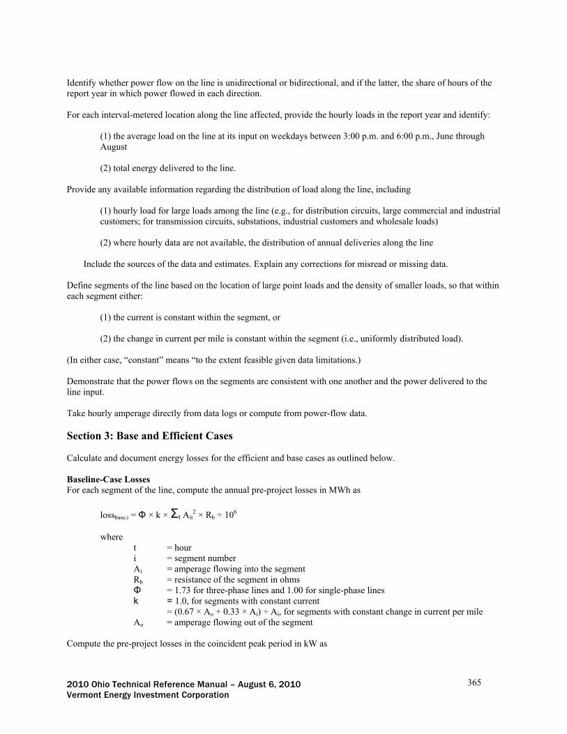
2010 Ohio Technical Reference Manual – August 6, 2010 365 Vermont Energy Investment Corporation
Identify whether power flow on the line is unidirectional or bidirectional, and if the latter, the share of hours of the report year in which power flowed in each direction. For each interval-metered location along the line affected, provide the hourly loads in the report year and identify:
(1) the average load on the line at its input on weekdays between 3:00 p.m. and 6:00 p.m., June through August (2) total energy delivered to the line.
Provide any available information regarding the distribution of load along the line, including
(1) hourly load for large loads among the line (e.g., for distribution circuits, large commercial and industrial customers; for transmission circuits, substations, industrial customers and wholesale loads) (2) where hourly data are not available, the distribution of annual deliveries along the line
Include the sources of the data and estimates. Explain any corrections for misread or missing data. Define segments of the line based on the location of large point loads and the density of smaller loads, so that within each segment either:
(1) the current is constant within the segment, or (2) the change in current per mile is constant within the segment (i.e., uniformly distributed load).
(In either case, “constant” means “to the extent feasible given data limitations.) Demonstrate that the power flows on the segments are consistent with one another and the power delivered to the line input. Take hourly amperage directly from data logs or compute from power-flow data. Section 3: Base and Efficient Cases Calculate and document energy losses for the efficient and base cases as outlined below. Baseline-Case Losses For each segment of the line, compute the annual pre-project losses in MWh as
lossbase,i = Φ × k × Σt Ait2 × Rb ÷ 106
where t = hour i = segment number Ai = amperage flowing into the segment Rb = resistance of the segment in ohms Φ = 1.73 for three-phase lines and 1.00 for single-phase lines k = 1.0, for segments with constant current = (0.67 × Ao + 0.33 × Ai) ÷ Ai, for segments with constant change in current per mile Ao = amperage flowing out of the segment
Compute the pre-project losses in the coincident peak period in kW as

2010 Ohio Technical Reference Manual – August 6, 2010 366 Vermont Energy Investment Corporation
peaklossbase,i = Φ × k × Σh Aih2 × Rb ÷ H ÷ 103
where h = hour in the coincident peak period H = number of hours in the coincident peak period
Provide manufacturer’s specifications, test results, or standard-reference data for the conductor for Rb. Provide the spreadsheet in which the base losses are computed. If this project consists of the incremental decrease of resistance for a new or replacement line, provide information demonstrating that the assumed base efficiency is in fact standard practice, including:
Current Industry Practice – Document current industry practice using articles from industry journals, manufacturers’ sales data, recent distribution standards from other utilities, and/or similar sources.
Applicant Practice – Document the utility’s own recent standard practices through purchase records, distribution standards, and similar documents. Provide data on peak forecasts for the line, supporting the adequacy of the base conductor.
If this project consists of the retrofit of lower-loss conductor solely for loss reductions,
Describe the existing conductor that was replaced.
Provide information demonstrating that the existing conductor could have remained in service. Document that the existing conductor was functioning properly. Provide certification that the existing conductor was adequate to meet anticipated loads. Describe the disposition of the existing conductor. Describe the manner in which the line was selected for retrofit, and provide documentation to demonstrate that the retrofit was undertaken for loss reduction, rather than actual or imminent failure or inadequacy.
Efficient-Case Losses For each segment of the line, compute the annual post-project losses in MWh as
lossefficient,i = Φ × k × Σt Ait2 × Re ÷ 106
where t = hour i = segment number Ai = amperage flowing into the segment Re = resistance of the segment in ohms Φ = 1.73 for three-phase lines and 1.00 for single-phase lines k = 1.0, for segments with constant current = (0.67 × Ao + 0.33 × Ai) ÷ Ai, for segments with constant change in current per mile Ao = amperage flowing out of the segment
Compute the post-project losses in the coincident peak period in kW as
peaklossefficient,i = Φ × k × Σh Aih2 × Re ÷ H ÷ 103

2010 Ohio Technical Reference Manual – August 6, 2010 367 Vermont Energy Investment Corporation
Provide manufacturer’s specifications, test results, or standard-reference data for the conductor for Re. Provide the spreadsheet in which the efficient-case losses are computed. Savings
Energy Savings = Σi(lossbase,i – lossefficient,i) × (1 + TELF) where TELF = Transmission Energy Loss Factor applicable to the transmission system upstream from
the project
Peak Savings = Σi (peaklossbase,i – peaklossefficient,i) × (1 + TPLF) where TPLF = Transmission Peak Loss Factor applicable to the transmission system upstream from
the project
If the utility has estimates of load-related losses on the transmission system, and uses those estimates in screening customer end-use efficiency measures, it may add those losses to the load reduction due to efficiency improvements on primary distribution lines. For transmission lines, the utility may compute TLF as the portion of transmission losses attributable to voltages equal to or higher than those of the input voltage to the project line. Provide the derivation of the estimate of transmission losses, and demonstrate the consistency of the claimed losses with the loss values used for the savings behind the customer meter. Section 4: Screening Inputs Measure Life Document the life of each type of added equipment, including reference to the utility’s depreciation studies. The efficient case analysis is typically performed over the lifetime of the major components. Where some equipment has a useful life shorter than the analysis period, describe the assumptions regarding the replacement cost of equipment with lives shorter than the analysis period. Where the utility would make a similar investment in the foreseeable future to meet peak load or reliability requirements, including the need to replace aging conductor, the analysis period should be limited to the period prior to that need date, and reflect the present value of the differences in capital costs. Operations Effects The estimates of baseline and efficiency case losses should reflect the operating practices be expected to be in place for the base and efficient conductors. O&M Cost Effects Include any foreseeable changes in O&M costs related to the change in conductor (including the effect of replacing old conductor with new conductor) and to any changes in operating practices. Cost Document the actual cost of the project, including equipment, internal and contract labor, allocated overheads, design, engineering, and permitting.

2010 Ohio Technical Reference Manual – August 6, 2010 368 Vermont Energy Investment Corporation
VI. Appendices A. Prototypical Building Energy Simulation Model Development B. Custom Analysis Template C. Documentation Summary Worksheet for Custom Projects D. TRM Maintenance and Update Process

2010 Ohio Technical Reference Manual – August 6, 2010 369 Vermont Energy Investment Corporation
Appendix A – Prototypical Building Energy Simulation Model Development Many of the savings values from the TRM are derived from DOE-2.2 simulations of typical commercial buildings. These prototypes were originally developed for the TRM document filed jointly by the Ohio electric utilities (Technical Reference Manual (TRM) for Ohio Senate Bill 221, Energy Efficiency and Conservation Program and 09-512-GE-UNC, October 15, 2009). They are based on building prototypes originally developed to calculate savings for California’s Database for Energy Efficient Resources (DEER), with certain parameters adjusted to Ohio building practice based on Duke Energy program experience and a review of the U.S. Energy Information Administration’s (EIA) Commercial Buildings Energy Consumption Survey (CBECS). The following sections provide a description of the prototypical buildings and a summary of key modeling assumptions. Commercial Building Prototype Model Development Commercial sector prototype building models were developed for a series of small commercial buildings with packaged rooftop HVAC systems, including assembly, big box retail, fast food restaurant, full service restaurant, grocery, light industrial, primary school, small office and small retail buildings. A large office prototype was also included to analyze measures associated with built-up HVAC systems. The following sections describe the prototypical simulation models used in this analysis. Assembly A prototypical building energy simulation model for an assembly building was developed using the DOE-2.2 building energy simulation program. The characteristics of the prototype are summarized in Table 11.
Table 11. Assembly Prototype Building Description Characteristic Value Vintage Existing (1970s) vintage Size 34,000 square feet
Auditorium: 33,240 SF Office: 760 SF
Number of floors 1 Wall construction and R-value Concrete block, R-5 Roof construction and R-value Wood frame with built-up roof, R-12 Glazing type Multipane Shading-coefficient = 0.84
U-value = 0.72 Lighting power density Auditorium: 1.9 W/SF
Office: 1.55 W/SF Plug load density Auditorium: 1.2 W/SF
Office: 1.7 W/SF Operating hours Mon-Sun: 8am – 9pm HVAC system type Packaged single zone, no economizer HVAC system size Based on ASHRAE design day conditions, 10% over
sizing assumed. Thermostat setpoints Occupied hours: 75 cooling, 70 heating
Unoccupied hours: 80 cooling, 65 heating A computer-generated sketch of the prototype is shown in Figure 2.

2010 Ohio Technical Reference Manual – August 6, 2010 370 Vermont Energy Investment Corporation
Figure 2. Assembly Building Rendering
Big Box Retail A prototypical building energy simulation model for a big box retail building was developed using the DOE-2.2 building energy simulation program. The characteristics of the prototype are summarized in Table 12.
Table 12. Big Box Retail Prototype Building Description Characteristic Value Vintage Existing (1970s) vintage Size 130,500 square feet
Sales: 107,339 SF Storage: 11,870 SF Office: 4,683 SF Auto repair: 5,151 SF Kitchen: 1,459 SF
Number of floors 1 Wall construction and R-value Concrete block with insulation, R-7.5 Roof construction and R-value Metal frame with built-up roof, R-13.5 Glazing type Multipane; Shading-coefficient = 0.84
U-value = 0.72 Lighting power density Sales: 2.15 W/SF
Storage: 0.85 W/SF (Active) 0.45 W/SF (Inactive) Office: 1.55 W/SF Auto repair: 1.7 W/SF Kitchen: 2.2 W/SF
Plug load density Sales: 1.15 W/SF Storage: 0.23 W/SF Office: 1.73 W/SF Auto repair: 1.15 W/SF Kitchen: 3.23 W/SF
Operating hours Mon-Sun: 10am – 9pm HVAC system type Packaged single zone, no economizer

2010 Ohio Technical Reference Manual – August 6, 2010 371 Vermont Energy Investment Corporation
Characteristic Value HVAC system size Based on ASHRAE design day conditions, 10% over
sizing assumed. Thermostat setpoints Occupied hours: 75 cooling, 70 heating
Unoccupied hours: 80 cooling, 65 heating A computer-generated sketch of the prototype is shown in Figure 3.
Figure 3. Big Box Retail Building Rendering
Fast Food Restaurant A prototypical building energy simulation model for a fast food restaurant was developed using the DOE-2.2 building energy simulation program. The characteristics of the prototype are summarized in Table 13.
Table 13. Fast Food Restaurant Prototype Building Description Characteristic Value Vintage Existing (1970s) vintage Size 2000 square feet
1000 SF dining 600 SF entry/lobby 300 SF kitchen 100 SF restroom
Number of floors 1 Wall construction and R-value Concrete block with brick veneer, R-7.5 Roof construction and R-value Concrete deck with built-up roof, R-13.5 Glazing type Multipane Shading-coefficient = 0.84
U-value = 0.72 Lighting power density Dining: 1.7 W/SF
Entry area: 1.7 W/SF Kitchen: 2.2 W/SF Restroom: 0.9 W/SF
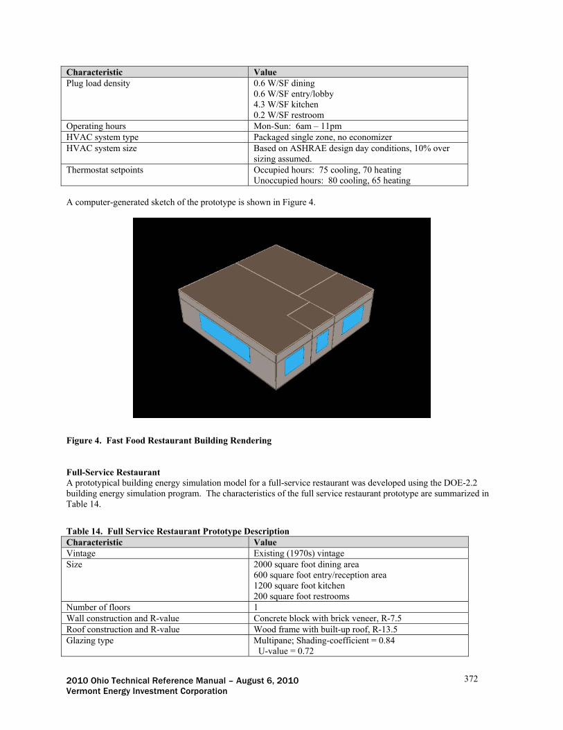
2010 Ohio Technical Reference Manual – August 6, 2010 372 Vermont Energy Investment Corporation
Characteristic Value Plug load density 0.6 W/SF dining
0.6 W/SF entry/lobby 4.3 W/SF kitchen 0.2 W/SF restroom
Operating hours Mon-Sun: 6am – 11pm HVAC system type Packaged single zone, no economizer HVAC system size Based on ASHRAE design day conditions, 10% over
sizing assumed. Thermostat setpoints Occupied hours: 75 cooling, 70 heating
Unoccupied hours: 80 cooling, 65 heating A computer-generated sketch of the prototype is shown in Figure 4.
Figure 4. Fast Food Restaurant Building Rendering Full-Service Restaurant A prototypical building energy simulation model for a full-service restaurant was developed using the DOE-2.2 building energy simulation program. The characteristics of the full service restaurant prototype are summarized in Table 14.
Table 14. Full Service Restaurant Prototype Description Characteristic Value Vintage Existing (1970s) vintage Size 2000 square foot dining area
600 square foot entry/reception area 1200 square foot kitchen 200 square foot restrooms
Number of floors 1 Wall construction and R-value Concrete block with brick veneer, R-7.5 Roof construction and R-value Wood frame with built-up roof, R-13.5 Glazing type Multipane; Shading-coefficient = 0.84
U-value = 0.72

2010 Ohio Technical Reference Manual – August 6, 2010 373 Vermont Energy Investment Corporation
Characteristic Value Lighting power density Dining area: 1.7 W/SF
Entry area: 1.7 W/SF Kitchen: 2.2 W/SF Restrooms: 1.5 W/SF
Plug load density Dining area: 0.6 W/SF Entry area: 0.6 W/SF Kitchen: 3.1 W/SF Restrooms: 0.2 W/SF
Operating hours 9am – 12am HVAC system type Packaged single zone, no economizer HVAC system size Based on ASHRAE design day conditions, 10% over
sizing assumed. Thermostat setpoints Occupied hours: 75 cooling, 70 heating
Unoccupied hours: 80 cooling, 65 heating A computer-generated sketch of the full-service restaurant prototype is shown in Figure 5.
Figure 5. Full Service Restaurant Prototype Rendering
Grocery A prototypical building energy simulation model for a grocery building was developed using the DOE-2.2 building energy simulation program. The characteristics of the prototype are summarized in Table 15.
Table 15. Grocery Prototype Building Description Characteristic Value Vintage Existing (1970s) vintage Size 50,000 square feet
Sales: 40,000 SF Office and employee lounge: 3,500 SF Dry storage: 2,860 SF 50 F prep area: 1,268 SF 35 F walk-in cooler: 1,560 SF

2010 Ohio Technical Reference Manual – August 6, 2010 374 Vermont Energy Investment Corporation
Characteristic Value - 5 F walk-in freezer: 812 SF
Number of floors 1 Wall construction and R-value Concrete block with insulation, R-5 Roof construction and R-value Metal frame with built-up roof, R-12 Glazing type Single pane clear Lighting power density Sales: 3.36 W/SF
Office: 2.2 W/SF Storage: 1.82 W/SF 50F prep area: 4.3 W/SF 35F walk-in cooler: 0.9 W/SF - 5F walk-in freezer: 0.9 W/SF
Equipment power density Sales: 1.15 W/SF Office: 1.73 W/SF Storage: 0.23 W/SF 50F prep area: 0.23 W/SF + 36 kBtu/hr process load 35F walk-in cooler: 0.23 W/SF + 17 kBtu/hr process load - 5F walk-in freezer: 0.23 W/SF+ 29 kBtu/hr process load
Operating hours Mon-Sun: 6am – 10pm HVAC system type Packaged single zone, no economizer Refrigeration system type Air cooled multiplex Refrigeration system size Low temperature (-20F suction temp): 23 compressor
ton Medium temperature (18F suction temp): 45 compressor ton
Refrigeration condenser size Low temperature: 535 kBtu/hr THR Medium temperature: 756 kBtu/hr THR
Thermostat setpoints Occupied hours: 74F cooling, 70F heating Unoccupied hours: 79F cooling, 65F heating
A computer-generated sketch of the prototype is shown in Figure 6.
Figure 6. Grocery Building Rendering

2010 Ohio Technical Reference Manual – August 6, 2010 375 Vermont Energy Investment Corporation
Large Office A prototypical building energy simulation model for a large office building was developed using the DOE-2.2 building energy simulation program. The characteristics of the prototype are summarized in Table 16.
Table 16. Large Office Prototype Building Description Characteristic Value Vintage Existing (1970s) vintage Size 350,000 square feet Number of floors 10 Wall construction and R-value Glass curtain wall, R-7.5 Roof construction and R-value Built-up roof, R-13.5 Glazing type Multipane; Shading-coefficient = 0.84
U-value = 0.72 Lighting power density Perimeter offices: 1.55 W/SF
Core offices: 1.45 W/SF Plug load density Perimeter offices: 1.6 W/SF
Core offices: 0.7 W/SF Operating hours Mon-Sat: 9am – 6pm
Sun: Unoccupied HVAC system types 1. Central constant volume system with perimeter hydronic reheat,
without economizer; 2. Central constant volume system with perimeter hydronic reheat, with economizer; 3. Central VAV system with perimeter hydronic reheat, with economizer
HVAC system size Based on ASHRAE design day conditions, 10% over sizing assumed. Chiller type Water cooled and air cooled Chilled water system type Constant volume with 3 way control valves, Chilled water system control Constant CHW Temp, 45 deg F setpoint Boiler type Hot water, 80% efficiency Hot water system type Constant volume with 3 way control valves, Hot water system control Constant HW Temp, 180 deg F setpoint Thermostat setpoints Occupied hours: 75 cooling, 70 heating
Unoccupied hours: 80 cooling, 65 heating Each set of measures was run using each of three different HVAC system configurations – a constant volume reheat system without economizer, a constant volume reheat system with economizer and a VAV system with economizer. The constant volume reheat system without economizer represents system with the most heating and cooling operating hours, while the VAV system with economizer represents a system with the least heating and cooling hours. This presents a range of system loads and energy savings for each measure analyzed. A computer-generated sketch of the prototype is shown in Figure 7. Note, the middle floors, since they thermally equivalent, are simulated as a single floor, and the results are multiplied by 8 to represent the energy consumption of the 8 middle floors.

2010 Ohio Technical Reference Manual – August 6, 2010 376 Vermont Energy Investment Corporation
Figure 7. Large Office Building Rendering Light Industrial A prototypical building energy simulation model for a light industrial building was developed using the DOE-2.2 building energy simulation program. The characteristics of the prototype are summarized in Table 17.
Table 17. Light Industrial Prototype Building Description Characteristic Value Vintage Existing (1970s) vintage Size 100,000 square feet total
80,000 SF factory 20,000 SF warehouse
Number of floors 1 Wall construction and R-value Concrete block with Brick, no insulation, R-5 Roof construction and R-value Concrete deck with built-up roof, R-12 Glazing type Multipane; Shading-coefficient = 0.84
U-value = 0.72 Lighting power density Factory – 2.25 W/SF
Warehouse – 0.7 W/SF Plug load density Factory – 1.2 W/SF
Warehouse – 0.2 W/SF Operating hours Mon-Fri: 6am – 6pm
Sat Sun: Unoccupied HVAC system type Packaged single zone, no economizer HVAC system size Based on ASHRAE design day conditions, 10% over
sizing assumed. Thermostat setpoints Occupied hours: 75 cooling, 70 heating
Unoccupied hours: 80 cooling, 65 heating A computer-generated sketch of the prototype is shown in Figure 8.

2010 Ohio Technical Reference Manual – August 6, 2010 377 Vermont Energy Investment Corporation
Figure 8. Light Industrial Building Rendering Primary School A prototypical building energy simulation model for an elementary school was developed using the DOE-2.2 building energy simulation program. The model is really of two identical buildings oriented in two different directions. The characteristics of the prototype are summarized in Table 18.
Table 18. Elementary School Prototype Building Description Characteristic Value Vintage Existing (1970s) vintage Size 2 buildings, 25,000 square feet each; oriented 90 from
each other Classroom: 15,750 SF Cafeteria: 3,750 SF Gymnasium: 3,750 SF Kitchen: 1,750 SF
Number of floors 1 Wall construction and R-value Concrete with brick veneer, R-7.5 Roof construction and R-value Wood frame with built-up roof, R-13.5 Glazing type Multipane Shading-coefficient = 0.84
U-value = 0.72 Lighting power density Classroom: 1.8 W/SF
Cafeteria: 1.3 W/SF Gymnasium: 1.7 W/SF Kitchen: 2.2 W/SF
Plug load density Classroom: 1.2 W/SF Cafeteria: 0.6 W/SF Gymnasium: 0.6 W/SF Kitchen: 4.2 W/SF
Operating hours Mon-Fri: 8am – 6pm Sun: 8am – 4pm
HVAC system type Packaged single zone, no economizer

2010 Ohio Technical Reference Manual – August 6, 2010 378 Vermont Energy Investment Corporation
Characteristic Value HVAC system size Based on ASHRAE design day conditions, 10% over
sizing assumed. Thermostat setpoints Occupied hours: 75 cooling, 70 heating
Unoccupied hours: 80 cooling, 65 heating A computer-generated sketch of the prototype is shown in Figure 9.
Figure 9. School Building Rendering
Small Office A prototypical building energy simulation model for a small office was developed using the DOE-2.2 building energy simulation program. The characteristics of the small office prototype are summarized in Table 19.
Table 19. Small Office Prototype Building Description Characteristic Value Vintage Existing (1970s) vintage Size 10,000 square feet Number of floors 2 Wall construction and R-value Wood frame with brick veneer, R-7.5 Roof construction and R-value Wood frame with built-up roof, R-13.5 Glazing type Multipane; Shading-coefficient = 0.84
U-value = 0.72 Lighting power density Perimeter offices: 1.55 W/SF
Core offices: 1.45 W/SF Plug load density Perimeter offices: 1.6 W/SF
Core offices: 0.7 W/SF Operating hours Mon-Sat: 9am – 6pm
Sun: Unoccupied HVAC system type Packaged single zone, no economizer HVAC system size Based on ASHRAE design day conditions, 10% over
sizing assumed.

2010 Ohio Technical Reference Manual – August 6, 2010 379 Vermont Energy Investment Corporation
Characteristic Value Thermostat setpoints Occupied hours: 75 cooling, 70 heating
Unoccupied hours: 80 cooling, 65 heating A computer-generated sketch of the small office prototype is shown in Figure 10.
Figure 10. Small Office Prototype Building Rendering Small Retail A prototypical building energy simulation model for a small retail building was developed using the DOE-2.2 building energy simulation program. The characteristics of the small retail building prototype are summarized in Table 20.
Table 20. Small Retail Prototype Description Characteristic Value Vintage Existing (1970s) vintage Size 6400 square foot sales area
1600 square foot storage area 8000 square feet total
Number of floors 1 Wall construction and R-value Concrete block with brick veneer, R-7.5 Roof construction and R-value Wood frame with built-up roof, R-13.5 Glazing type Multipane; Shading-coefficient = 0.84
U-value = 0.72 Lighting power density Sales area: 2.15 W/SF
Storage area: 0.85 W/SF (Active) 0.45 W/SF (Inactive)
Plug load density Sales area: 1.2 W/SF Storage area: 0.2 W/SF
Operating hours 10 – 10 Monday-Saturday 10 – 8 Sunday
HVAC system type Packaged single zone, no economizer HVAC system size Based on ASHRAE design day conditions, 10% over
sizing assumed.

2010 Ohio Technical Reference Manual – August 6, 2010 380 Vermont Energy Investment Corporation
Characteristic Value Thermostat setpoints Occupied hours: 75 cooling, 70 heating
Unoccupied hours: 80 cooling, 65 heating A computer-generated sketch of the small retail building prototype is shown in Figure 11.
Figure 11. Small Retail Prototype Building Rendering Weighting of Results The simulation models provide results at a level of detail that sometimes surpass the normal data collection procedures from customer incentive applications and other EDC data collection. Thus, weights were assigned to individual simulation results, and the weighted averages were reported in the TRM sections where the added complexity of using building type-specific factors was unwarranted. The weights used for analysis were derived from Duke Energy data. For the commercial building analysis, the weights assigned to each of the building types are shown below:
Table 21. Commercial Building Type Weights Building Type Weight Assembly 0.118 Big Box 0.017 Fast food 0.017 Full Service 0.042 Light industrial 0.008 Primary school 0.059 Small office 0.176 Small retail 0.563
Note, the large office and grocery store models were used to analyze specific measures unique to the HVAC system and equipment types used in these buildings. Results relevant to these building types were reported separately and not included in the weighted averages.

2010 Ohio Technical Reference Manual – August 6, 2010 381 Vermont Energy Investment Corporation
Appendix B – Custom Analysis Template A. Project Information779
Project Name Date
Project, measure, metering and analysis information shall reflect the project as installed and operating. Directions to the user of the template are in this font throughout the document. Analysts should use a different font to document the project information. Submit all required utility and/or PUCO documentation, the completed Custom Analysis Template and associated documentation as indicated herein and in the TRM. List project documentation in the Documentation Summary Worksheet (Appendix C).
This template complements the Technical Reference Manual requirements for custom measure analysis. Refer to the appropriate TRM protocol to ensure adequate documentation of the custom analysis. The Sections in this template are labeled A – E as they do not directly correspond to the four sections in the TRM.
Table 22
Program Name
Customer Name
Site Name if Different
Site Address
Building or Site Type
NAICS Code
Customer Business/Product
Building Size
Project Start Date
Start Date of Measure Installation
Project Completion Date
Applicable Codes &/or Standards
Electric Utility & Account Number
Meter Number
Annual Electric Energy Use on Affected Meter
Pre-installation Annual kWh: Pre-installation maximum billed kW:
779 Section A of this document is based on a Measurement and Verification Template developed by Energy Resource Solutions for NYSERDA in 2010.

2010 Ohio Technical Reference Manual – August 6, 2010 382 Vermont Energy Investment Corporation
Rate
Gas Utility & Account Number
Meter Number
Annual Gas Energy Use on Affected Meter Pre-installation Annual Consumption Therms:
Rate
Add rows as needed to provide the necessary information regarding any other energy sources are affected by this project (ie. Fuel oil or renewable energy) Principal Customer Contact Name
Title
Phone
Utility Representative Name
Title
Phone
Custom Energy Analyst Contact Technical lead for this custom analysis.
Name
Title
Company
Phone Office: Cell:
Mailing Address
Additional Project Contact
Role
Title
Company
Phone
Add lines as needed
Project Description Describe the project and how it saves energy. Complete the following Project Savings Summary table based on the results of the savings analysis per Section D below.
Table 23 – Project Savings Summary
Measure
Number Measure Name
Electic Energy Savings
(kWh/yr)
Coincident Demand Savings
(kW)
Gas Savings (therms/yr)
Other Fuel Impacts
1
2

2010 Ohio Technical Reference Manual – August 6, 2010 383 Vermont Energy Investment Corporation
Measure
Number Measure Name
Electic Energy Savings
(kWh/yr)
Coincident Demand Savings
(kW)
Gas Savings (therms/yr)
Other Fuel Impacts
3
Total Savings for All Measures
Add information regarding other fuel impacts if the project impacts unregulated fuels such as fuel oil, renewable, etc. and indicate units in the header. Delete columns that are not applicable to the project, except electric efficiency projects must include Electric Energy and Coincident Demand columns. Add rows as needed to address all measures associated with the project. Show any increases in energy as a result of the project as a negative number (negative savings).
B. Measure Information Document the following information for each project measure. Duplicate Section B for each unique measure. Include all information necessary to describe the equipment and how it operates, including manufacturer’s information. Reference case studies of similar systems wherever possible. Reference supporting documentation in the Documentation Summary Worksheet. Duplicate the following sections as needed.
Measure Number and Name Measure Description
Describe the new technology, measure, and/or change in operations, and how it saves energy.
Measure Performance in Comparison with Relevant Codes and Standards Document the relevant efficiency codes or federal/state/local standards that apply to the proposed efficient equipment and the ratings of the measure equipment in comparison with applicable standards.
Additional Benefits If the efficient measure was the result of a process improvement that provides additional benefits, such as waste reduction, clearly describe all of the ways that the new process saves energy and resources. This can include reductions in areas such as waste heat, O&M costs, labor costs, water consumption, or process waste.
Baseline Description Describe the baseline condition. Reference the TRM requirements. Complete Documentation Summary Worksheet to document industrial process baselines for retrofit projects.
Relevant Codes and Standards For New Construction and Equipment Replacement Projects the Baseline is the applicable code and/or standard. Clearly cite the reference code or standard used to

2010 Ohio Technical Reference Manual – August 6, 2010 384 Vermont Energy Investment Corporation
establish baseline efficiency levels including year of issue, chapters or sections referenced for the project and the specific requirements of the code and/or standard and how it was applied in the project analysis. If this information is fully documented under Section B.1.1, reference that section here.
Measure Variables Describe the variables that impact project energy use, the impacts of the measure on any of the variables and how the values for the variables and energy use were established. Common variables are listed below, add or delete as needed to accurately describe the variables associated with the measure. Add quantitative information regarding the project variables in Table 24 - Measure Variables. Document all equipment information for the sections below using the Documentation Summary Worksheet.
Equipment Loading Describe the equipment loading, variations in loading, percent loading and load profiles during the performance hours.
Operating Conditions
Seasonal and Daily Variability in Schedule Describe any seasonality that affects the measure (production, school schedules, etc.) Provide documentation of data sources and assumptions used in the analysis.
Production For industrial process measures, document units of production used for baseline and efficient cases, product variations included and the daily and seasonal variation in production.
Weather Describe any weather dependence of the measure.
Controls Describe equipment controls, any differences in baseline and efficiency case controls and how control sequences are accounted for in the analysis.
Interactive Effects Describe interactive effects including waste heat, additional heating required and interactions with other measures or systems that will impact energy consumption.
Measure Life State recommended measure life and reference for basis of recommendation.

2010 Ohio Technical Reference Manual – August 6, 2010 385 Vermont Energy Investment Corporation
Table 24 - Measure Variables
Variable Applies (Y/N) Values Used and Engineering Units Source (eg. metering, customer interview, production log, etc.)
Equipment Loading
Operating Schedules
Production Schedules
Occupancy Schedules
Weather
Production
Controls
Interactive Effects
C. Metering and Data Collection
Prepare a metering plan for the project using this section of the document and indicating the intended analysis approach in Section D. Upon completion of metering and analysis, update this document to reflect actual findings and final analysis approach.
Metering Approach Discuss the approach to energy and demand metering including load shape and coincident demand determination from meter data. Describe when metering occurred and how it is deemed to represent the post installation, annual operating conditions. Provide justification and supporting documentation for all assumptions and metering techniques using the Documentation Summary Worksheet.
Data Collection Methodology Indicate the primary method(s) used to obtain the data needed for TRM Section 2 equations.
Power Metering
Data logging
DDC/PLC
Interval Data
Customer Interview

2010 Ohio Technical Reference Manual – August 6, 2010 386 Vermont Energy Investment Corporation
Other (describe)
Table 25 - Project Data Acquisition
Data Collection Method [1]
When data was collected (pre/post) installation
Measure(s) Affected
Equipment monitored
Parameter measured
Measurement equipment
Observation frequency
Metering duration
Sensor type
Accuracy of sensors
Overall accuracy of meter system
Verify whether meter was synchronized to NIST
[1] Indicate data collection method(s) across the top; not all rows apply for all data collection methods. Duplicate table as needed to capture all data collection methods used for the measures associated with this project
Equipment Calibration Discuss calibration procedures used to maintain calibration of any metering and/or logging equipment used in the metering process. Where DDC and/or PLC devices and systems were used to obtain project data, describe the calibration protocol and document the results in the Documentation Summary Worksheet.
Data Cleaning and Data Reduction Discuss steps taken to align timestamps, fill gaps in raw data and address other data issues such as inaccurate or inconclusive readings. Depending on the level of verification required by the program, include raw, cleaned, and analyzed datasets as appropriate in the Documentation Summary Worksheet.

2010 Ohio Technical Reference Manual – August 6, 2010 387 Vermont Energy Investment Corporation
D. Energy and Demand Analysis
Energy and Demand Analysis Approach Describe the energy and demand savings calculation approach for each measure. Present formulae; the basis for each variable should be documented in Sections B and C above. If modeling is used, describe the simulation tool and modeling approach. Describe the approach to determining the coincident demand savings for electric efficiency measures. All project and measure analysis documentation shall be submitted as part of the project documentation in the Documentation Summary Worksheet.
Calculation Methods Describe the calculation methods and tools used to develop the savings analysis for the project. Include a discussion of how interactive effects were handled in the analysis. Refer to the TRM for more details on interactive effects.
Computer Modeling Describe the approach to computer modeling, software used including, year, version and source, the modeling parameters addressed and the confidence in the model results relative to predictions of annual energy use reduction. Document the software year, version, source, and supporting documentation for software algorithms in the Documentation Summary Worksheet.
Energy and Demand Savings Analysis Complete this section for each of the measures named above in accordance with Sections 2 through 4 of the C&I Custom Measure TRM for Retrofit and/or Equipment Replacement and report the final results in the Projects Savings Summary in Section A above. Perform the savings analysis according to the following algorithm.
Step 1. Enter the system description and conditions into Table 27 using the example below as a guide. Include all modes of operation that occur throughout the course of a year. For variable loads and schedules, enter ‘variable’ in the Hours, Coincidence Factor, and Load Factors columns.
Table 26 - System Conditions Example

2010 Ohio Technical Reference Manual – August 6, 2010 388 Vermont Energy Investment Corporation
Table 27 - System Description - Measure 1 J Subsystem Hours Coincidence
Factor System mode Full load kW
[1] Load Factor
[2] 1 2 3 4 5 6 7 8 9
10 11
[1] Nameplate kW. [2] Typically less than 1.00 unless the equipment was sized to run at full speed.
Step 2. Use the equations in TRM Section 2 to calculate the following quantities in Table 28 - Calculated Energy Consumption and Demand Summary below: Energyeff, Energybase, C Loadeff, C Loadbase and the corresponding savings Energysaved and C Loadsaved. Where the Hours, Coincidence Factor, and Load Factor are variable in Step 1 above, such as for weather dependent systems or other variable loads and schedules, a comprehensive 8760 analysis approach is required for affected terms in the equations. For subsystems ‘J’ which are constant and fully defined in the table above, it is acceptable to calculate these terms directly without using an 8760 analysis.
Table 28 - Calculated Energy Consumption and Demand Summary [1]
Baseline Case Efficient Case Annual Energy Savings
Notes
Measure 1
Annual Energy Use Electric
Coincident Electric Demand
Annual Gas Use
Measure 2
Annual Energy Use Electric
Coincident Electric Demand
Annual Gas Use
[1] Add rows for additional measures and for reporting impacts on unregulated energy sources. Indicate NA if a listed energy source is not affected. Electric measures must have both energy and coincident demand analysis completed.

2010 Ohio Technical Reference Manual – August 6, 2010 389 Vermont Energy Investment Corporation
E. Additional Information Provide supporting documentation for all information referenced in Section E using the Documentation Summary Worksheet.
Project Cost Document the cost of each measure by supplying electronic copies of quotes and invoices. For equipment replacement and new construction projects, the measure cost is the incremental cost above the baseline equipment. For retrofit projects the cost is inclusive.
Table 29 - Calculated Cost [1]
Baseline Case
(leave blank for Retrofit)
Efficient Case Incremental Cost of Efficient Measure
(total inclusive cost for Retrofit)
Notes
Measure 1
Measure 2
Measure 3
[1] Add rows for additional measures.
Nonenergy Impacts Document the non-energy impacts of the project such as impacts on O&M, water consumption etc. and the costs associated with those impacts.
Uncertainty Discuss sources of uncertainty in energy use and demand reduction calculations other than metering error. Address assumption and potential impact of deviations in actual conditions from assumed conditions on energy savings. Discuss deviations from the original metering plan and quantify the impacts on the calculated savings.
Accuracy The overall engineering accuracy of this analysis is: +/-________ %
Signature of Energy Analyst
Date of Submitted Report

2010 Ohio Technical Reference Manual – August 6, 2010 390 Vermont Energy Investment Corporation
Appendix C – Documentation Summary Worksheet for Custom Projects
Appendix A
Documentation Summary Worksheet for Custom Projects
Instructions:
5. Provide files listed in this table in electronic format with the project submission.
Section Category Subcategory Efficent Baseline
Section A ‐ Project Information
Custom Analysis Template
Section B ‐ Measure Level
Reference Data and Studies
Applicable Codes or Standards
Case Studies and Industry StandardsApplicant Practice (Industrial Retrofit)
Equipment Specific Information
Manufacturer Performance DataNameplate Data
Operating VariablesField Metered Load Data
Section C ‐ Metering and Data Collection
Metering TechniquesCalibration Logs (DDC)
Metering DatasetsAnalyzed
Raw†Cleaned†
Section D ‐ Energy and Demand Analysis
Analysis FilesModeling Files
Calculations Spreadsheets
Savings
Savings Analysis CalculationsSavings Equations Source
Section E ‐ Additional Information
Project CostsNon‐Energy Impacts
† Raw and Cleaned datasets are not typically required for savings claims However, they should be available to Program Evaluation staff if requested.
Filename with Extension
(.pdf, .xlsx, .inp, etc.)
Case to which documentation
appliesDocumentation Requirements
Measure(s) to which
documentation applies
Description
4. Indicate filenames of submitted documents in Column H. Include the measure number in the filename.
1. Documentation is required for all sections and subsections shown in Columns A ‐ C. Add rows as needed in order to completely document the project according to the
requirements of the applicable Custom TRM and the Custom Analysis Template.
2. Indicate by "X" in columns D & E whether the documentation applies to the Baseline, Efficient or Both cases.
3. Indicate the measures to which the documentation applies in Column F, such as "M‐1, M‐2…". Use "P" for documentation that applies to the overall project.
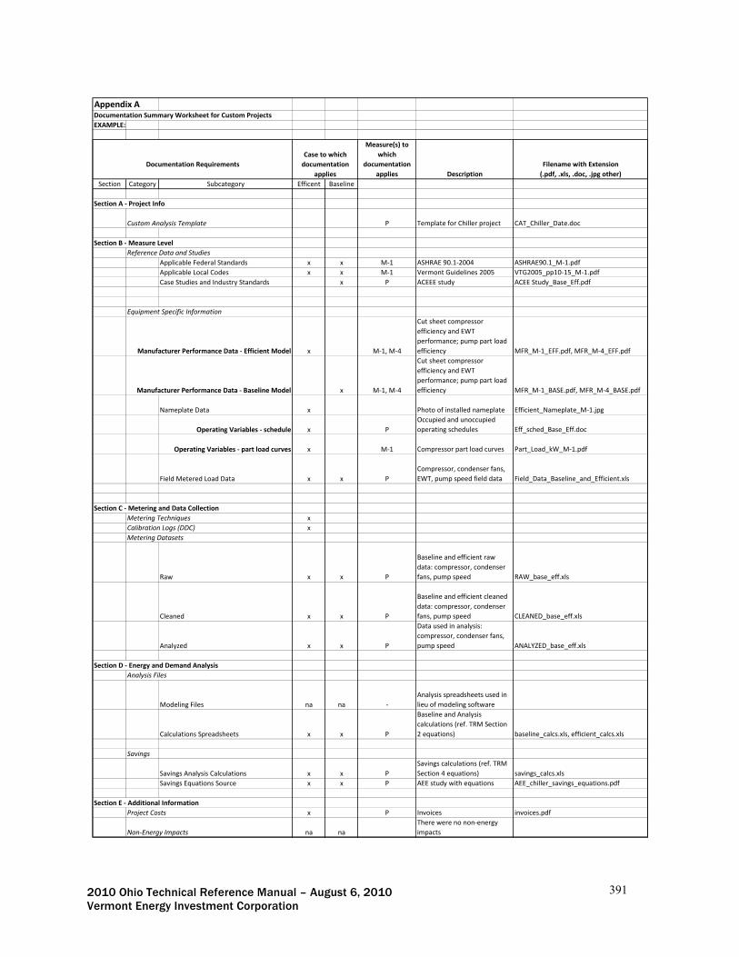
2010 Ohio Technical Reference Manual – August 6, 2010 391 Vermont Energy Investment Corporation
Appendix ADocumentation Summary Worksheet for Custom Projects
EXAMPLE:
Measure(s) to
which
documentation
applies Description
Filename with Extension
(.pdf, .xls, .doc, .jpg other)
Section Category Subcategory Efficent Baseline
Section A ‐ Project Info
Custom Analysis Template P Template for Chiller project CAT_Chiller_Date.doc
Section B ‐ Measure Level
Reference Data and Studies
Applicable Federal Standards x x M‐1 ASHRAE 90.1‐2004 ASHRAE90.1_M‐1.pdf
Applicable Local Codes x x M‐1 Vermont Guidelines 2005 VTG2005_pp10‐15_M‐1.pdf
Case Studies and Industry Standards x P ACEEE study ACEE Study_Base_Eff.pdf
Equipment Specific Information
Manufacturer Performance Data ‐ Efficient Model x M‐1, M‐4
Cut sheet compressor
efficiency and EWT
performance; pump part load
efficiency MFR_M‐1_EFF.pdf, MFR_M‐4_EFF.pdf
Manufacturer Performance Data ‐ Baseline Model x M‐1, M‐4
Cut sheet compressor
efficiency and EWT
performance; pump part load
efficiency MFR_M‐1_BASE.pdf, MFR_M‐4_BASE.pdf
Nameplate Data x Photo of installed nameplate Efficient_Nameplate_M‐1.jpg
Operating Variables ‐ schedule x P
Occupied and unoccupied
operating schedules Eff_sched_Base_Eff.doc
Operating Variables ‐ part load curves x M‐1 Compressor part load curves Part_Load_kW_M‐1.pdf
Field Metered Load Data x x P
Compressor, condenser fans,
EWT, pump speed field data Field_Data_Baseline_and_Efficient.xls
Section C ‐ Metering and Data Collection
Metering Techniques x
Calibration Logs (DDC) x
Metering Datasets
Raw x x P
Baseline and efficient raw
data: compressor, condenser
fans, pump speed RAW_base_eff.xls
Cleaned x x P
Baseline and efficient cleaned
data: compressor, condenser
fans, pump speed CLEANED_base_eff.xls
Analyzed x x P
Data used in analysis:
compressor, condenser fans,
pump speed ANALYZED_base_eff.xls
Section D ‐ Energy and Demand Analysis
Analysis Files
Modeling Files na na ‐
Analysis spreadsheets used in
lieu of modeling software
Calculations Spreadsheets x x P
Baseline and Analysis
calculations (ref. TRM Section
2 equations) baseline_calcs.xls, efficient_calcs.xls
Savings
Savings Analysis Calculations x x P
Savings calculations (ref. TRM
Section 4 equations) savings_calcs.xls
Savings Equations Source x x P AEE study with equations AEE_chiller_savings_equations.pdf
Section E ‐ Additional Information
Project Costs x P Invoices invoices.pdf
Non‐Energy Impacts na na
There were no non‐energy
impacts
Documentation Requirements
Case to which
documentation
applies

2010 Ohio Technical Reference Manual – August 6, 2010 392 Vermont Energy Investment Corporation
Appendix D – TRM Maintenance and Update Process The Ohio Technical Reference Manual is designed to be a living document – it will benefit from an objective and thoughtful update process. Defining a process that coordinates with the needs of users, evaluators, and regulators is critical. Below we outline a process for the update of information and recommendations on the coordination of the timing of this process with other critical activities. Proposed TRM Update Process Once a TRM has been developed, it is vital that it is kept up to date, appended, and maintained in a timely and effective manner. There are three main points in time when a TRM is most likely to require changes:
New measure additions – As new technologies become cost effective, they will need to be characterized and added to the manual. In addition, new program delivery design may result in the need for new measure characterization.
Existing measure updates – Updates will be required for a number of reasons. Examples include: the federal standard for efficiency of a measure is increased; the qualification criteria are altered; the measure cost falls; or a new evaluation provides a better value of an assumption for a variable. In addition, as programs mature, characterizations need to be updated as changes in the market require changes in calculation assumptions. In such cases, these changes must be identified and appropriate changes made to the TRM.
Retiring existing measures – When the economics of a measure become such that it is no longer cost effective, or the free rider rate is so high that it is not worth supporting, the measure should be retired.
It is important to maintain a record of changes made to the TRM over time. It is therefore recommended to establish and maintain a Master Manual, containing all versions of each TRM in chronological order, and an abridged User Manual, in which only the current versions of active measures are included. Archiving older information in this fashion can be designed into the electronic interface (if developed), and only the current version of the User Manual is publically available on the site. The flowchart presented below outlines steps that will result in effective review and quality control for TRM updates. One critical component is the establishment of a Technical Advisory Group (TAG) to provide a forum for discussing and resolving technical concerns. This process requires a number of different roles to ensure effectiveness, sufficient review, and independence. The specific parties who will hold these roles in the Ohio TRM maintenance context will be clarified in discussion with the Commission. The following list of key responsibilities is given as a starting place for this conversation:
Program administrators / utilities (consultants)
o Identifies need for new or revised measure characterization – usually due to program changes or program/market feedback
o Researches and develop first draft measure characterizations – for needs that the utilities identify
o Develops second draft measure characterizations following feedback on first draft from all parties
o Gives feedback on draft measure characterizations from other parties
o Participates in Technical Advisory Group (TAG) for formal discussion and dispute resolution when needed
o Gives input to regulators if TAG process does not resolve all issues

2010 Ohio Technical Reference Manual – August 6, 2010 393 Vermont Energy Investment Corporation
Flowchart for Proposed TRM Update Process
Step Responsible Party
1Identify Need for Addition or
ModificationProgram Administrator, Evaluator, and/or TRM Manager
2Develop 1st Draft of New Measure Characterization Party that identified need
3Circulate 1st Draft to Other
Parties/Stakeholders Party that drafts
4Informal feedback on 1st
Draft All stakeholders
5Revised 1st draft based on feedback and recirculate TRM Manager
Consensus Proposal Disagreement
6 Formal TAG mtg All stakeholders
Disagreement
7 Decision/Approval Regulators
8 Update TRM TRM Manager
Process Flow
Independent TRM Manager (Consultant)
o Identifies need for revised measure characterization (usually based on knowledge of local or other relevant evaluation studies)
o Researches and develops first draft measure characterizations – for needs identified either by itself or Evaluation consultant
o Gives feedback on first draft measure characterizations from other parties
o Develops second draft measure characterizations following feedback on first draft from all parties
o Leads Technical Advisory Group (TAG) for formal discussion and dispute resolution when needed
o Provides input to regulators if TAG process does not resolve all issues

2010 Ohio Technical Reference Manual – August 6, 2010 394 Vermont Energy Investment Corporation
o Makes recommendation for TRM revision to PUCO
o Manages and updates TRM manuals (after PUCO approval of changes)
Third-party Evaluation consultant
o Identifies need for revised measure characterization (usually based on local evaluation studies it has conducted or managed)
o Input on draft measure characterizations developed by other parties
o Participates in TAG meetings when appropriate
o Performs program evaluation - includes statewide market assessment and baseline studies, savings impact studies (to measure the change in energy and / or demand use attributed to energy efficiency), and other energy efficiency program evaluation activities
o Verifies annual energy and capacity savings claims of each program and portfolio
o Ensures proper utility use of TRM in annual savings verification process
Commission staff
o Hires and manages TRM and Evaluation consultant(s)
o Approves any changes to TRM – includes serving as final arbiter in any disagreements between utilities and TRM consultant
The process outlined above also assumes that there are several potential stages of “give and take” on draft modifications to the TRM. At a minimum, there is at least one round of informal feedback and comment between the program administrators and the independent reviewer (TRM Manager or otherwise). Other parties could be invited to participate in this process as well. In the event that such informal discussions do not resolve all issues, the participants may find it beneficial to establish a Technical Advisory Group (TAG) to provide a more formal venue for resolution of technical disputes prior to any submission to the regulators. This group would include representation from the program administrators, the evaluators (when deemed useful), the TRM Manager, and Commission staff. The mission of such a group would be to discuss and reach agreement on any unresolved issues stemming from new measure proposals, savings verifications, or evaluations. They could also review and comment on the methodology and associated assumptions underlying measure savings calculations and provide an additional channel for transparency of information about the TRM and the savings assessment process. Coordination with Other Savings Assessment Activities As drafted, the Ohio Administrative Code requires the Commission/Staff to report whether an electric utility’s or mercantile customer’s actions match their proposed program portfolio; whether the utility’s or mercantile customer’s proposed program portfolio would produce actual savings; and whether actual savings were achieved. Although the TRM will be a critically important tool for both DSM planning and estimation of actual savings, it will not, by itself, ensure that reported savings are the same as actual savings. There are two principal reasons for this:
1. The TRM itself does not ensure appropriate estimation of savings. One of the responsibilities of the Independent Program Evaluator will be to assess that the TRM has been used appropriately in the calculation of savings.
2. The TRM may have assumptions or protocols that new information suggests are outdated. New information that could inform the reasonableness of TRM assumptions or protocols can surface at any time, but they are particularly common as local evaluations or annual savings verification processes are completed. Obviously, the TRM should be updated to reflect such new information. However, it is highly likely that some such adjustments will be made too late to affect the annual savings estimate of a utility or mercantile customer for the previous year, particularly given the PUCO’s interim decision to not adjust savings estimates retroactively (TRM Entry Appendix A). Thus, there may be a difference between savings estimates in annual compliance reports and the “actual savings” that the PUCO may consider acceptable from a regulatory perspective. However, such updates should be captured in as timely a fashion as possible.

2010 Ohio Technical Reference Manual – August 6, 2010 395 Vermont Energy Investment Corporation
These two issues highlight the fact that the TRM needs to be integrated into a broader process that has two other key components: an annual savings verification process and on-going evaluation. Savings verification ensures that information is being tracked accurately and in a manner consistent with the TRM. However, as important as it is, verification does not ensure that reported savings are “actual savings”. TRMs are never and can never be perfect. Even when the verification process documents that assumptions have been appropriately applied, it can also highlight questions that warrant future analysis that may lead to changes to the TRM. Put another way, evaluation studies are and always will be necessary to identify changes that need to be made to the TRM. Therefore, in addition to annual savings verification processes, evaluations will periodically be made to assess or update the underlying assumption values for critical components of important measure characterizations. In summary, there should be a strong, sometimes cyclical relationship between the TRM development and update process, annual compliance reports, savings verification processes, and evaluations. As such, we recommend coordinating these activities. A preliminary timeline established from such a coordinated process is given in the table below.
Annual Verification and TRM Update Timeline Jan Feb Mar Apr May Jun Jul Aug Sep Oct Nov Dec
Draft annual savings report
No TRM submittal during SV
Draft new or updated measure characterizations developed and submitted
to TRM Manager; participate in TAG Utility
SV response Prior year data finalized
Savings verification
(SV)
Technical Advisory Group (TAG) negotiations and evaluation
Evaluator
No TRM review
during SV Refers need for TRM updates to TRM
Manager; provides input on characterizations
TRM Manager
No TRM during
savings verification Propose/develop new or updated measure characterizations; review drafts provided
by utilities; participate in TAG
PUCO
Make final savings
determination
Participate in TAG meetings; approve final TRM
In this example, it assumed that updates to the TRM occur only in the second half of the year. One option is to establish two specific update deadlines: one in September and the other at the end of December. The first would ensure that the best available data are available for utility planning for the following year. The second would ensure that best available assumptions are in place prior to the start of the new program year. In general, we would expect the number of additions or revisions in the September TRM update to be much greater than the number in December. Nevertheless, providing for two rounds of TRM review each year gives the opportunity to have updated savings assumptions reviewed and approved more often, reducing the time that a program administrator might be at risk of providing services using not-yet-approved measure characterizations. The rationale for not updating the TRM during the first half of the year is that time is usually devoted, in part, to documenting, verifying and approving savings claims from the previous year. For example, the program administrator will likely require two months to produce its annual savings claim for the previous year. An independent reviewer will then require two to three months to review and probe that claim, with considerable back and forth between the two parties being very

2010 Ohio Technical Reference Manual – August 6, 2010 396 Vermont Energy Investment Corporation
common. Typically, final savings estimates for the previous year are not finalized and approved until mid-year. Program administrators and evaluators would be unlikely to have the time or focus for considering changes to measure characterizations during this time.