static analysis of arch bridge_thesis
DESCRIPTION
STATIC ANALYSIS OF ARCH BRIDGESTRANSCRIPT


ii

Statical Analysisof
Network Arch Bridges
October 7th, 2009 – April 7th 2010
Author Alejandro Jose NiklisonMatr.-Nr.:2542427
1st Supervisor Prof. Dr.-Ing. habil. Manfred BischoffInstitute of Structural MechanicsUniversität StuttgartPfaffenwaldring 7, 70550 StuttgartGermany
2nd Supervisor Dipl. -Ing. (FH) Annika Sorg, M. Sc.Institute of Structural MechanicsUniversität StuttgartPfaffenwaldring 7, 70550 StuttgartGermany
iii

iv
Abstract
The primary topic of this dissertation is the study of different parameters that influence the
structural behavior of network arch bridges. As a particular example the bridge over the
river Lužnice in the Czech Republic is examined.
First, a simplified static computation of the Lužnice bridge is presented, along with different
assumptions regarding the elements, materials and loading of the bridge. The worst loading
conditions are determined.
Considering this, four different parameters are studied: the hanger arrangement, the form of
the arch, the rise of the arch and the number of hangers.
As the hanger arrangement constitutes the main characteristic of network arch bridges,
special emphasis is placed on this parameter. In particular, two hanger arrangements are
analyzed: A configuration based on the linear variation of the slopes and a radial
arrangement, proposed by Brunn and Schanack in their diploma thesis [BSC].
Different shapes of the arch are proposed and studied, as well as modifications in the rise
of the arch and the number of hangers.
Finally, different alternatives are proposed and compared with the original configurations of
the bridge over the river Lužnice.
v

vi

Declaration
I, Mr. Alejandro José Niklison, declare that this master´s thesis is written independently and
no sources have been used other than the stated referenced.
…...................................... …........................................Place/Date Signature
vii

viii

MASTER THESIS – MASTER OF SCIENCE IN COMPUTATIONAL MECHANICS
STATICAL ANALYSIS OF NETWORK ARCH BRIDGES
UNIVERSITÄT STUTTGART – INSTITUT FÜR BAUSTATIK UND BAUDYNAMIK
2010
Contents
Abstract v
Declaration vii
List of Figures xiii
List of Tables xxi
Nomenclature xxiii
1 Introduction 11.1. Network Arch Bridges 11.2. Structural Outline 5
2 Computation of the bridge over the river Lužnice 72.1. General Configuration 72.2. Elements 8
2.2.1. Arch 82.2.2. Deck 102.2.3. Hangers 11
2.3. Type of materials 132.3.1. Arch 132.3.2. Deck 132.3.3. Hangers 13
2.4 Load Analysis 142.4.1. Verification at Ultimate Limit States 142.4.2. Actions 15
2.4.2.1 Permanent Actions 152.4.2.2 Presstresing 162.4.2.3 Traffic loads 162.4.2.4 Combination of Actions 192.4.2.5 Load Cases 22
2.5 Prestresing of the cables 222.6 Results 23
2.6.1 Deck 232.6.1.1 Even Load 232.6.1.2 Partial load 26
2.6.2 Arch 282.6.2.1 Even Load 282.6.2.2 Partial load 31
2.6.3 Hangers 332.6.3.1 Even Load 332.6.3.2 Partial load 34
2.7 Conclusions 35
3 Study of parameters 373.1 Hanger Arrengement 38
PÁG.
ix

MASTER THESIS – MASTER OF SCIENCE IN COMPUTATIONAL MECHANICS
STATICAL ANALYSIS OF NETWORK ARCH BRIDGES
UNIVERSITÄT STUTTGART – INSTITUT FÜR BAUSTATIK UND BAUDYNAMIK
2010
3.1.1 Linear Variation of the Slopes 383.1.1.1 Results 39
3.1.1.1.1Bending moments in thedeck 39
3.1.1.1.2 Axial forces in the deck 423.1.1.1.3 Stresses in the deck 44
3.1.1.1.4Bending moments in thearch 47
3.1.1.1.5 Axial forces in the arch 483.1.1.1.6 Stresses in the arch 513.1.1.1.7 Stresses in the hangers 533.1.1.1.8 Relaxed hangers 55
3.1.1.2 Conclusions 553.1.2 Radial arrengement 58
3.1.2.1 Results 59
3.1.2.1.1Bending moments in thedeck 59
3.1.2.1.2 Axial forces in the deck 613.1.2.1.3 Stresses in the deck 63
3.1.2.1.4Bending moments in thearch 66
3.1.2.1.5 Axial forces in the arch 683.1.2.1.6 Stresses in the arch 713.1.2.1.7 Stresses in the hangers 743.1.2.1.8 Relaxed hangers 76
3.1.2.2 Conclusions 773.2 Shape of the arch 79
3.2.1 Results 803.2.1.1 Bending moments in the deck 803.2.1.2 Axial forces in the deck 833.2.1.3 Stresses in the deck 863.2.1.4 Bending moments in the arch 883.2.1.5 Axial forces in the arch 903.2.1.6 Stresses in the arch 933.2.1.7 Stresses in the hangers 953.2.1.8 Relaxed hangers 96
3.2.2 Conclusions 983.3 Rise of the arch 100
3.3.1 Results 1003.3.1.1 Bending moments in the deck 1003.3.1.2 Axial forces in the deck 1013.3.1.3 Stresses in the deck 1023.3.1.4 Bending moments in the arch 1033.3.1.5 Axial forces in the arch 1043.3.1.6 Stresses in the arch 1053.3.1.7 Stresses in the hangers 1063.3.1.8 Relaxed hangers 107
3.3.2 Conclusions 1073.4 Number of hangers 108
PÁG.
x

MASTER THESIS – MASTER OF SCIENCE IN COMPUTATIONAL MECHANICS
STATICAL ANALYSIS OF NETWORK ARCH BRIDGES
UNIVERSITÄT STUTTGART – INSTITUT FÜR BAUSTATIK UND BAUDYNAMIK
2010
3.4.1 Results 1083.4.1.1 Bending moments in the deck 1083.4.1.2 Axial forces in the deck 1093.4.1.3 Stresses in the deck 1103.4.1.4 Bending moments in the arch 1113.4.1.5 Axial forces in the arch 1123.4.1.6 Stresses in the arch 1133.4.1.7 Stresses in the hangers 1143.4.1.8 Relaxed hangers 115
3.4.2 Conclusions 1164 Study of alternatives 117
4.1 Proposed Configurations 1174.1.1 Original Configuration 1174.1.2 Alternative A 1174.1.3 Alternative B 1184.1.4 Alternative C 119
4.2 Comparison of Alternatives 1204.2.1 Stresses in the deck 1204.2.2 Stresses in the arch 1214.2.3 Stresses in the hangers 122
4.3 Conclusions 125
5 Summary 127
A Appendix A. Sections of the Lužnice Bridge 129
B Appendix B. Results for the Lužnice Bridge 131
C Appendix C. Numbers assigned to hanger elements 141
D Appendix D. Input File 143D.1 Preliminary Definitions 143D.2 Definition of Parameters 143
D.2.1 Geometry and dimensions 143D.2.1.1 Deck 143D.2.1.2 Arch 144D.2.1.3 Hangers 144
D.2.2 Material and Loading properties 144D.2.3 Cross angles for the Radial Arrengement 145D.2.4 Definition of Matrices 145
D.3 Geometry of the bridge 146D.3.1 Loop 146D.3.2 Geometry of arch and deck 146D.3.3 Hanger arrengement 147D.3.4 Enhancement of the model 148
D.3.4.1 Deck 148D.3.4.2 Arch 150D.3.4.3 Hangers 151
D.4 Boundary conditions 152
PÁG.
xi

MASTER THESIS – MASTER OF SCIENCE IN COMPUTATIONAL MECHANICS
STATICAL ANALYSIS OF NETWORK ARCH BRIDGES
UNIVERSITÄT STUTTGART – INSTITUT FÜR BAUSTATIK UND BAUDYNAMIK
2010
D.5 Elements and sections 152D.6 Loads 153
D.6.1 Preliminary Definitions 153D.6.2 Load steps 154
D.6.2.1 LM1. Distributed load 154D.6.2.2 LM1. Puntual loads 155D.6.2.3 Dead Load 156
D.6.2.3.1 Dead Load. Unfavorable 156D.6.2.3.2 Dead Load. Favorable 157
D.7 Solution 158D.7.1 Preliminary Definitions 158D.7.2 Elements Output definitions 158D.7.3 Definition of load cases 159D.7.4 Storage of the results 160
D.7.4.1 Hangers 160D.7.4.2 Arch 161D.7.4.3 Deck 163
D.7.5 Matrices 165
Bibliography 167
PÁG.
xii

MASTER THESIS – MASTER OF SCIENCE IN COMPUTATIONAL MECHANICS
STATICAL ANALYSIS OF NETWORK ARCH BRIDGES
UNIVERSITÄT STUTTGART – INSTITUT FÜR BAUSTATIK UND BAUDYNAMIK
2010
List of Figures
1 Arch bridge with vertical hangers – Even Load [TNA] 2
2 Arch bridge with vertical hangers – Partial Load [TNA] 2
3 Areas, stiffnesses and influence lines for the lower and upper chord of two tied archs [TNA] 3
4 Bridge over the river Lužnice close to Bechyně in the Czech Republic 3
5 Erection of the Lužnice network arch bridge [TNA] 4
6 Element BEAM3 [Hlp] 8
7 Cross Section of the arch 9
8 Effective wide [DIN] 10
9 Effective span [DIN] 10
10 Cross Section of deck 11
11 Element LINK10 12
12 Cross Section Hangers 12
13 Aditional permanent actions 15
14 Load Model 1 [E1-2] 17
15 Load Model 2 [E1-2] 18
16 Loads on footpaths [E1-2] 18
17 Details of LM1 (Transversal and longitudinal) 19
18 Details of LM2 (Transversal and longitudinal) 20
19 Details of LM4 (Transversal and longitudinal) 21
20 Axial forces for the deck elements of the of the Lužnice bridge(Even load) 24
21 Moments for the deck elements of the Lužnice bridge (Even load) 25
22 Stresses for the deck elements of the Lužnice bridge (Even load) 25
PÁG.
xiii

MASTER THESIS – MASTER OF SCIENCE IN COMPUTATIONAL MECHANICS
STATICAL ANALYSIS OF NETWORK ARCH BRIDGES
UNIVERSITÄT STUTTGART – INSTITUT FÜR BAUSTATIK UND BAUDYNAMIK
2010
23 Axial forces for the deck elements of the of the Lužnice bridge(Partial Load). 27
24 Moments for the deck elements of the Lužnice bridge (Partial Load) 27
25 Stresses for the deck elements of the Lužnice bridge (Partial Load) 28
26 Axial forces for the arch elements of the of the Lužnice bridge (Even load) 29
27 Moments for the arch elements of the Lužnice bridge (Even load) 30
28 Stresses for the arch elements of the Lužnice bridge (Even load) 30
29 Axial forces for the arch elements of the of the Lužnice bridge (Partial Load) 32
30 Moments for the arch elements of the Lužnice bridge (Partial load) 32
31 Stresses for the arch elements of the Lužnice bridge (Partial load) 33
32 Stresses for hangers of the Lužnice bridge (Full Load) 34
33 Stresses for hangers of the Lužnice bridge (Partial Load) 35
34 Arrangement of the hangers based on the linear variationof the slopes 38
35 Maximum bending moments in the deck (Linear variation ofthe slopes) 39
36 Hanger arrangement for ϕ0= 84° - ∆ϕ = 0.0° 39
37 Hanger arrangement for ϕ0= 70° - ∆ϕ�= 3.2° 40
38 Corresponding X-coordinates for the maximum bending momentsin the deck (Linear variation of the slopes) 41
39 Corresponding load cases for the maximum bending moments inthe deck (Linear variation of the slopes) 41
40 Maximum axial forces in the deck (Linear variation of the slopes) 42
41 Hanger arrangement for ϕ0= 65° - ∆ϕ�= 3.4° 43
42 Corresponding X-coordinates for the maximum axial forces in the deck (Linear variation of the slopes) 43
PÁG.
xiv

MASTER THESIS – MASTER OF SCIENCE IN COMPUTATIONAL MECHANICS
STATICAL ANALYSIS OF NETWORK ARCH BRIDGES
UNIVERSITÄT STUTTGART – INSTITUT FÜR BAUSTATIK UND BAUDYNAMIK
2010
43 Corresponding load cases for the maximum bending moments in the deck (Linear variation of the slopes ) 44
44 Maximum stresses in the deck (Linear variation of the slopes) 45
45 Corresponding X-coordinate for the maximum stresses in the deck (Linear variation of the slopes) 46
46 Corresponding load cases for the maximum stresses in the deck(Linear variation of the slopes) 46
47 Maximum bending moments in the arch (Linear variation of the slopes) 47
48 Corresponding X-coordinate for the maximum bending moments in the arch (Linear variation of the slopes) 48
49 Maximum axial compression forces in the arch (Linear variation of the slopes) 49
50 Corresponding X-coordinate for the maximum axial compression forces in the arch (Linear variation of the slopes) 50
51 Corresponding load cases for the maximum axial compression forces in the arch (Linear variation of the slopes) 50
52 Maximum stresses in the arch (Linear variation of the slopes) 51
53 Hanger arrangement for ϕ0= 70° - ∆ϕ�= 0.0° 52
54 Hanger arrangement for ϕ0= 73° - ∆ϕ�= 3.0° 52
55 Corresponding X-coordinate for the maximum stresses in the arch(Linear variation of the slopes) 52
56 Maximum stresses in the hangers (Linear variation of the slopes) 53
57 Number of relaxed hangers (Linear variation of the slopes) 54
58 Hanger arrangement for ϕ0= 65° - ∆ϕ =0.0° 55
59 Number of times the hangers intersect each other in each bridge 55
60 Deformations for hanger arrangements with ϕ0= 65° - ∆ϕ = 0.0° 57
61 Deformations for hanger arrangements with ϕ0= 65° - ∆ϕ = 3.4° 57
62 Radial arrangement [BSC] 58
PÁG.
xv

MASTER THESIS – MASTER OF SCIENCE IN COMPUTATIONAL MECHANICS
STATICAL ANALYSIS OF NETWORK ARCH BRIDGES
UNIVERSITÄT STUTTGART – INSTITUT FÜR BAUSTATIK UND BAUDYNAMIK
2010
63 Radial arrangement. The adopted variable is the angle marked as grey [BSC] 58
64 Maximum bending moments in the deck (Radial arrangement) 59
65 Radial arrangement. Cross angle = 45° 59
66 Corresponding X-coordinates for the maximum bending momentsin the deck (Radial arrangement) 60
67 Corresponding load cases for the maximum bending moments in the deck (Radial arrangement) 61
68 Maximum axial forces in the deck (Radial arrangement) 62
69 Corresponding X-coordinates for the maximum axial forcesin the deck (Radial arrangement) 62
70 Corresponding load cases for the maximum axial forces in the deck (Radial arrangement) 63
71 Maximum stresses in the deck (Radial arrangement) 64
72 Corresponding X-coordinates for the maximum stresses in the deck (Radial arrangement) 65
73 Corresponding load cases for the maximum stresses in the deck (Radial arrangement) 65
74 Maximum bending moments in the arch (Radial arrangement) 66
75 Radial arrangement. Cross angle = 47.5° 66
76 Corresponding X-coordinates for the maximum bending moments in the arch (Radial arrangement) 67
77 Corresponding load cases for the maximum bending momentsin the arch (Radial arrangement) 68
78 Maximum axial compression forces in the arch (Radial arrangement) 69
79 Radial arrangement. Cross angle = 0° 69
80 Corresponding X-coordinates for the maximum axial compression forces in the arch (Radial arrangement) 70
81 Corresponding load cases for the maximum axial compression forces in the arch (Radial arrangement) 71
PÁG.
xvi

MASTER THESIS – MASTER OF SCIENCE IN COMPUTATIONAL MECHANICS
STATICAL ANALYSIS OF NETWORK ARCH BRIDGES
UNIVERSITÄT STUTTGART – INSTITUT FÜR BAUSTATIK UND BAUDYNAMIK
2010
82 Maximum stresses in the arch (Radial arrangement) 72
83 Corresponding X-coordinates for the maximum stresses in the arch (Radial arrangement) 73
84 Corresponding load cases for the maximum stresses in the arch (Radial arrangement) 73
85 Maximum stresses in the hangers (Radial arrangement) 74
86 Corresponding elements for the maximum stresses in the hangers (Radial arrangement) 75
87 Corresponding load cases for the maximum stresses in the hangers (Radial arrangement) 76
88 Number of relaxed hangers (Radial arrangement) 77
89 Variables used to described the shape of the arch 79
90 Hanger arrangement for ϕ0= 70° - ∆ϕ�= 1.0° 79
91 Maximum bending moments in the deck (Shape of the arch) 81
92 Arch shape: Rrel=3.0 ; long1 = 0.05 81
93 Arch shape: Rrel=1.0 ; long1 = 0.50 81
94 Corresponding X-coordinates for the maximum bending moments in the deck (Shape of the arch) 82
95 Corresponding load cases for the maximum bending moments in the deck (Shape of the arch) 83
96 Maximum axial forces in the deck (Shape of the arch) 84
97 Corresponding X-coordinates for the maximum axial forces in the deck (Shape of the arch) 85
98 Corresponding load cases for the maximum axial forces in the deck (Shape of the arch) 85
99 Maximum stresses in the deck (Shape of the arch) 86
100 Corresponding X-coordinates for the maximum stresses inthe deck (Shape of the arch) 87
PÁG.
xvii

MASTER THESIS – MASTER OF SCIENCE IN COMPUTATIONAL MECHANICS
STATICAL ANALYSIS OF NETWORK ARCH BRIDGES
UNIVERSITÄT STUTTGART – INSTITUT FÜR BAUSTATIK UND BAUDYNAMIK
2010
101 Corresponding load cases for the maximum stresses in the deck (Shape of the arch) 88
102 Maximum bending moments in the arch (Shape of the arch) 89
103 Corresponding X-coordinates for the maximum bending moments in the arch (Shape of the arch) 89
104 Corresponding load cases for the maximum bending moments in the arch (Shape of the arch) 90
105 Maximum axial compression forces in the arch (Shape of the arch) 91
106 Arch shape: Rrel=3.0 ; long1 = 0.125 91
107 Corresponding X-coordinates for the maximum axial compression forces in the arch (Shape of the arch) 92
108 Corresponding load cases for the maximum axial compression forces in the arch (Shape of the arch) 92
109 Maximum stresses in the arch (Variation of the shape of the arch) 93
110 Corresponding X-coordinates for the maximum stresses in the arch (Shape of the arch) 94
111 Corresponding load cases for the maximum stresses in the arch (Shape of the arch) 94
112 Maximum stresses in the hangers (Shape of the arch) 95
113 Corresponding elements for the maximum stresses in thehangers (Variation of the shape of the arch) 96
114 Relaxed hangers (Shape of the arch) 97
115 Arch shape: Rrel=1.1 ; long1 = 0.075 97
116 Arch shape: Rrel= 1.2 ; long1 = 0.10 97
117 Maximum bending moments in the deck (Rise of the Arch) 101
118 Maximum axial forces in the deck (Rise of the Arch) 102
119 Maximum stresses in the deck (Rise of the Arch) 103
120 Maximum bending moments in the arch (Rise of the Arch) 104
PÁG.
xvii

MASTER THESIS – MASTER OF SCIENCE IN COMPUTATIONAL MECHANICS
STATICAL ANALYSIS OF NETWORK ARCH BRIDGES
UNIVERSITÄT STUTTGART – INSTITUT FÜR BAUSTATIK UND BAUDYNAMIK
2010
121 Maximum axial compression forces in the arch (Rise of the Arch) 105
122 Maximum stresses in the arch (Rise of the Arch) 106
123 Maximum stresses in the hangers (Rise of the Arch) 107
124 Maximum bending moments in the deck (Number of Hangers) 109
125 Maximum axial forces in the deck (Number of Hangers) 110
126 Maximum stresses in the deck (Number of Hangers) 111
127 Maximum bending moments in the arch (Number of Hangers) 112
128 Maximum axial compression forces in the arch (Number of Hangers) 113
129 Maximum stresses in the arch (Number of Hangers) 114
130 Maximum stresses in the hangers (Number of Hangers) 115
131 Relaxed hangers (Number of Hangers) 116
132 Alternative A 118
133 Alternative B 118
134 Alternative C 119
135 Comparison of Alternatives. Stresses in the deck 121
136 Comparison of Alternatives. Stresses in the arch 122
137 Comparison of Alternatives. Stresses in the hangers for the Set 1 124
138 Comparison of Alternatives. Stresses in the hangers for the Set 2 124
A.1 Cross section of the Lužnice Bridge 129
A.2 Longitudinal section of the Lužnice Bridge 130
C.1 Numbers assigned to hanger elements (Original hanger arrengement and hanger arrengements based on the linear variation of the slopes) 141
C.2 Numbers assigned to hanger elements (Radial arrengements) 141
D.1 Parameters SDIR, SBYT and SBYB 162
PÁG.
xix

MASTER THESIS – MASTER OF SCIENCE IN COMPUTATIONAL MECHANICS
STATICAL ANALYSIS OF NETWORK ARCH BRIDGES
UNIVERSITÄT STUTTGART – INSTITUT FÜR BAUSTATIK UND BAUDYNAMIK
2010
PÁG.
xx

MASTER THESIS – MASTER OF SCIENCE IN COMPUTATIONAL MECHANICS
STATICAL ANALYSIS OF NETWORK ARCH BRIDGES
UNIVERSITÄT STUTTGART – INSTITUT FÜR BAUSTATIK UND BAUDYNAMIK
2010
List of Tables
1 Values for a set of hangers of the Lužnice network arch bridge 8
B.1 Maximum and minimum bending moments and axial forces for the deck elements (Even Load) 121
B.2 Maximum and minimum stresses for the deck elements (Even Load) 132
B.3 Maximum and minimum bending moments and axial forces for the deck elements (Partial Load) 133
B.4Maximum and minimum stresses for the deck elements (PartialLoad) 134
B.5 Maximum and minimum bending moments and axial forces for the arch elements (Even Load) 135
B.6 Maximum and minimum stresses for the arch elements (Even Load) 136
B.7 Maximum and minimum bending moments and axial forces for the arch elements (Partial Load) 137
B.8Maximum and minimum stresses for the arch elements (PartialLoad) 138
B.9Maximum and minimum stresses for the hanger elements (EvenLoad) 139
B.10 Maximum and minimum stresses for the hanger elements (Partial Load) 140
PÁG.
xxi

MASTER THESIS – MASTER OF SCIENCE IN COMPUTATIONAL MECHANICS
STATICAL ANALYSIS OF NETWORK ARCH BRIDGES
UNIVERSITÄT STUTTGART – INSTITUT FÜR BAUSTATIK UND BAUDYNAMIK
2010
PÁG.
xxii

MASTER THESIS – MASTER OF SCIENCE IN COMPUTATIONAL MECHANICS
STATICAL ANALYSIS OF NETWORK ARCH BRIDGES
UNIVERSITÄT STUTTGART – INSTITUT FÜR BAUSTATIK UND BAUDYNAMIK
2010
Nomenclature
ϕ0 Initial Angle
∆ϕ Angle increment
M Bending Moments
N Axial Forces
S Stress
Coord Coordinates
Rrel Radio of the circular part of the arch
long1 Distance from where the parabolic shape begins
PÁG.
xxii

MASTER THESIS – MASTER OF SCIENCE IN COMPUTATIONAL MECHANICS
STATICAL ANALYSIS OF NETWORK ARCH BRIDGES
UNIVERSITÄT STUTTGART – INSTITUT FÜR BAUSTATIK UND BAUDYNAMIK
2010
PÁG.
xxiv

MASTER THESIS – MASTER OF SCIENCE IN COMPUTATIONAL MECHANICS
STATICAL ANALYSIS OF NETWORK ARCH BRIDGES
UNIVERSITÄT STUTTGART – INSTITUT FÜR BAUSTATIK UND BAUDYNAMIK
2010
Chapter 1
Introduction
1.1 Network Arch Bridges
Developed by the norwegian engineer Per Tveit in the end of the 1950s, the network archbridges are considered as the most slender and lightest arch bridges in the world.
Network arch bridges are arch bridges in which some of the hangers intersect othershangers at least twice. With an optimal design, the hangers act like a web of a simply supportedbeam in which the tie and the arch are the tensile and the compresive flanges respectively. Mostof the shear force is carried to the supports by the vertical components of the forces in the arch,and the variation in the shear force is taken by variations in the forces in the hangers. Because ofthis, the arch and the tie are mainly subjected to axial forces with reduced bending moments. Thisresults in very small sections and a slender and atractive bridge.
In order to achive an optimal design several consideration should be taken into account[TNA]:
− It is recommendable for the arch to be part of a circle, as this contributes to evenbending moments along the tie and to a more constant axial force in a longer portion ofthe arch. However, in this thesis other forms are investigated in Section 3.2.
− The upper nodes of the hangers should be equidistantly spaced along the arch.
− The lower nodes of the hangers should be placed in a way that the variation of themaximum forces in the hangers is minimum, and the relaxation of the hangers isavoided.
− The tie should be a concrete slab between concrete edge beams. As the bendingmoment in the middle of the span in usually bigger than the longitudinal bending, thereis no need for steel beams.
− The axial forces between the ends of the arches should be taken by longitudinalprestressing. Transversal prestressing is only necessary if the distance between edgebeams is more than 10.00 meters.
− All hangers should have the same cross section.
− Special attention should be dedicated to the choice of the hanger arrangement.Different hanger arrangements are examinated in Section 3.1.
Regarding the method of erection of network arch bridges, it is recommendable to use atemporary lower chord, whenever is possible. A steel skeleton can be built combining the lowerchord with the arches and the hangers in a suitable location. The skeleton can be moved to thefinal position with cranes [TNA].
The advantages of the Network arch bridges over the arches with vertical hangers areexposed next.
For evenly distributed loads an arch with vertical hangers could be a good solution, as allelements are mainly subjected to axial forces (Fig. 1). However, a partial load of the span will leadto a deflection of the arch and tie, increasing significantly the bending moments (Fig.2).
PÁG.
1

MASTER THESIS – MASTER OF SCIENCE IN COMPUTATIONAL MECHANICS
STATICAL ANALYSIS OF NETWORK ARCH BRIDGES
UNIVERSITÄT STUTTGART – INSTITUT FÜR BAUSTATIK UND BAUDYNAMIK
2010
Figure 1. Arch bridge with vertical hangers – Even Load [TNA]
Figure 2. Arch bridge with vertical hangers – Partial Load [TNA]
For the case of partial loading, the network arch bridge has a better structural response.For an optimal hanger arrangement, the loads are led to the arches such that there is littlebending in the chords. A high stiffness is attained and the deflections of the arch and tie arerestricted by the inclined hangers. The stiffness in the arch planes cause the deck to spanbetween them, without taking much longitudinal bending. In consequence it can be slender.
Figure 3 shows influence lines for bending moments between a bridge with verticalhangers and a network arch bridge [TNA]. The first bridge was built at Straubing in 1977. Thenetwork arch bridge was design by Per Tveit for the IABSE Congress in Vienna in 1980. In [TNA]Per Teat note that the maximum influence ordinate for the tie in the network arch is the same asfor a simply supported beam of 5.60 m of span. As the distance between the arches of the bridgeis 15.00 m, the bending moment in the tie is much smaller than the maximum bending moment inthe slab.
Observing the influence lines for the arches and the lower chords in Figure 3, it can benotice that the values for the network arch bridges are much smaller than the values for the bridgewith vertical hangers. It can also be notice that the form of the influence lines for the arch is quitesimilar to the form of the influence lines for the tie.
PÁG.
2

MASTER THESIS – MASTER OF SCIENCE IN COMPUTATIONAL MECHANICS
STATICAL ANALYSIS OF NETWORK ARCH BRIDGES
UNIVERSITÄT STUTTGART – INSTITUT FÜR BAUSTATIK UND BAUDYNAMIK
2010
Figure 3. Areas, stiffnesses and influence lines for the lower and upper chord of two tiedarches [TNA]
As a particular example for this thesis, the bridge over the river Lužnice, close to Bechyněin the Czech Republic is used (Fig. 4). This is the third network arch bridge in the world with steelarches and a prestressed concrete deck.
Figure 4. Bridge over the river Lužnice close to Bechyně in the Czech Republic [LIM]
PÁG.
3

MASTER THESIS – MASTER OF SCIENCE IN COMPUTATIONAL MECHANICS
STATICAL ANALYSIS OF NETWORK ARCH BRIDGES
UNIVERSITÄT STUTTGART – INSTITUT FÜR BAUSTATIK UND BAUDYNAMIK
2010
The 41.00 m, single-lane bridge replaced an old steel lattice bridge. As the setting calledfor a slender structure with an attractive appearance, the network arch was a good choice.
The bridge has two parabolic shaped steel arches, with an inverted U cross section, and amaximum height of 6.05 m. The cross sections are open to allow access for inspection andmaintenance. The arches are reinforced with transverse welded steel U beams in the end of thearches and in the one quarter and three quarters points.
The C35/C45 concrete deck is 7.95 m wide and with a thickness of 18 cm under thesidewalks, and 25 to 30 cm under the roadway. It is supported by 38 hangers distributed evenlyalongside each arch. It is prestressed by four steel cables embedded in the concrete slab. Thecables are anchored in vertical steel face plates at the end of each arch. As the wide of the deck isless than 10.00 m, it is not necessary transversal prestressing and the slab acts like reinforcedconcrete.
The hangers are stainless steel rods with an outside diameter of 40 mm. The hangersclose to the end of the arches need to be prestressed. The other hangers are prestressed by theweight of the deck.
The single traffic lane is 3.60 m, with sidewalks in both sides. Each sidewalk is 1.30 mwide and it is separated from the traffic lane by a steel guardrail that protects the hangers.
The pavement of the road consist of a medium-grained mastic asphalt carpet made ofmodified asphalt, poured asphalt and waterproofing, with a total thickness of 85 mm.
Before the erection of the bridge, the original bridge had to be moved to another location,placing it on a temporary support to allow the traffic to continue. The steel structure wasassembled on-site. It was erected without welding using a steel support scaffolding that wasplaced on temporary supports (Figure 5). Later, the steel skeleton was placed in the abutmentsusing hydraulic jacks. Once the deck was casted and cured, the hangers were adjusted. Afterprestressing the slab, the scaffolding was removed.
The Appendix A presents a cross section and a longitudinal section of the Lužnice bridge.
Figure 5. Erection of the Lužnice network arch bridge [TNA]
PÁG.
4

MASTER THESIS – MASTER OF SCIENCE IN COMPUTATIONAL MECHANICS
STATICAL ANALYSIS OF NETWORK ARCH BRIDGES
UNIVERSITÄT STUTTGART – INSTITUT FÜR BAUSTATIK UND BAUDYNAMIK
2010
1.2. Structural OutlineThis dissertation is organized in five parts:• A simplified statical computation of the Lužnice bridge is presented in Chapter 2. The
different assumptions referring the elements, material and actions in the bridge aredescribed extensively. Finally, an analysis of the results is exposed in order to find theworst load cases.
• Chapter 3 concentrates in the study of different parameters in order to determine theirinfluence in the structural behavior of the bridge. The parameters to study are the hangerarrangement, the form of the arch, the rise of the arch and the number of hangers.
• In the Chapter 4 different alternatives to the original configuration are proposed andanalyzed.
• The Chapter 5 provides a brief summary of the whole work.
PÁG.
5

MASTER THESIS – MASTER OF SCIENCE IN COMPUTATIONAL MECHANICS
STATICAL ANALYSIS OF NETWORK ARCH BRIDGES
UNIVERSITÄT STUTTGART – INSTITUT FÜR BAUSTATIK UND BAUDYNAMIK
2010
PÁG.
6

MASTER THESIS – MASTER OF SCIENCE IN COMPUTATIONAL MECHANICS
STATICAL ANALYSIS OF NETWORK ARCH BRIDGES
UNIVERSITÄT STUTTGART – INSTITUT FÜR BAUSTATIK UND BAUDYNAMIK
2010
Chapter 2
Computation of the bridge over the river Lužnice
In order to study the statical properties of network arch bridges, the bridge over the riverLužnice is chosen as an example. In this chapter a simplified 2D model of the bridge is calculated.As a special emphasis is placed on the difficulty with hangers that do not carry under compressiveforces, it is compulsive to do geometrically non-linear computations. For that it is necessary to useelements that do not carry under compressive forces.
For this reason, the finite element software ANSYS, in its version 12.0.1, is used, as it isable to model elements that do not contribute to carry the load when exposed to compressiveforces.
The bridge is modeled with beam elements, distinguishing between elements that onlycarry axial forces (hangers) and elements that carry also shear forces and bending moments(deck and arch).
The units used are meters (m), kilonewtons (KN), second (s) and tons (t).The Chapter 2 is divided in seven sections:•••• The general configuration of the bridge is exposed in Section 2.1 with a detail of the
hanger arrangement.
•••• The Sections 2.2 and 2.3 present the elements and type of material used for the deck,the arch and the hangers, along with its characteristics.
•••• The Section 2.4. presents the load analysis. In this section the different actions aredescribed, presenting the load models, the combination of actions and the load cases.
•••• The prestressing of the cables is described in the Section 2.5.
•••• In the Section 2.6. the results obtained from the models are analyzed. In order to findthe worst loading assumptions the maximum values for stress, bending moments andaxial forces are presented for each element, along with the corresponding load cases.This is done separately for the elements of hangers, deck and arch, and for an evenand a partial loading of the deck.
•••• Finally, the conclusions are exposed in the Section 2.7.
2.1 General Configuration
The arch has a parabolic shape. It begins in the origin of coordinates and it ends in thecoordinate (41.00 ; 0.00), as the span of the bridge is 41.00 m. It has its maximum ordinate in thecenter, with a value of 6.05 m.
For the left margin hinged supports are adopted. The hinged supports allow the rotation,while the translational displacement is not possible. In the right margin, it is considered rollersupports. In this case both rotation and translational displacement are allowed.
The Table 1 shows the angles and distances to the origin of one set of hangers. The other set of hangers is the mirrored equivalent.
PÁG.
7

MASTER THESIS – MASTER OF SCIENCE IN COMPUTATIONAL MECHANICS
STATICAL ANALYSIS OF NETWORK ARCH BRIDGES
UNIVERSITÄT STUTTGART – INSTITUT FÜR BAUSTATIK UND BAUDYNAMIK
2010
Table 1. Values for a set of hangers of the Lužnice network arch bridge
2.2 Elements
2.2.1 Arch
The arch is modeled with BEAM3 elements [AHlp]. These are uniaxial 2D elements withtension, compression and bending capabilities. The elements have three degrees of freedom ateach node: rotation about the nodal Z axis, and translation in the directions of the X and Y axis.Figure 6 shows the geometry and the coordinate system of the element.
Figure 6. Element BEAM3 [Hlp]
PÁG.
8
x [m] α [°]3.12 46.335.10 50.017.10 50.999.10 51.02
11.10 53.5913.00 55.1815.08 58.1317.07 60.4919.06 61.9221.07 62.7823.07 63.1625.07 63.1027.07 62.5829.07 61.5831.08 59.9533.08 59.6435.07 60.5437.09 56.4339.11 51.54

MASTER THESIS – MASTER OF SCIENCE IN COMPUTATIONAL MECHANICS
STATICAL ANALYSIS OF NETWORK ARCH BRIDGES
UNIVERSITÄT STUTTGART – INSTITUT FÜR BAUSTATIK UND BAUDYNAMIK
2010
Input data [AHlp]:
The BEAM3 element is defined by two nodes, the cross sectional area, the inertia moment,the height and the material properties. The cross section of the arch is illustrated in the Figure 7.The characteristics of the section are:
− Area: 0.3115 e-01 m2
− Inertia Moment: 0.3688 e-03 m3
− Height: 0.32 m
Figure 7. Cross Section of the arch
Output data [AHlp]:
The following results are extracted in order to study the structural behavior of the system:
The axial direct stress (SDIR) and the bending stresses (SBYT and SBYB) are combinedin order to obtain the maximum stress in each node.
PÁG.
9
SDIR-I Axial direct stress in node iSDIR-J Axial direct stress in node jSBYT-I Bending stress on the element +Y side of the beam, in node iSBYT-J Bending stress on the element +Y side of the beam, in node jSBYB-I Bending stress on the element -Y side of the beam, in node iSBYB-J Bending stress on the element -Y side of the beam, in node jMFORX-I Member force in the element coordinate system X direction, in node iMFORX-J Member force in the element coordinate system X direction, in node jMFORMZ-I Member moment in the element coordinate system Z direction, in node iMFORMZ-J Member moment in the element coordinate system Z direction, in node j

MASTER THESIS – MASTER OF SCIENCE IN COMPUTATIONAL MECHANICS
STATICAL ANALYSIS OF NETWORK ARCH BRIDGES
UNIVERSITÄT STUTTGART – INSTITUT FÜR BAUSTATIK UND BAUDYNAMIK
2010
2.2.2 Deck
The Deck is also modeled with BEAM3 elements (Figure 6) [AHlp].
Input data [AHlp]:
The BEAM3 element is defined by two nodes, the cross sectional area, the inertia moment,the height and the material properties.
In the deck a reduced cross section is adopted. This is due to the fact that point loads areapplied where the hangers meet the deck. This loads spread into the deck with a certain angle nottaking all the cross section. For this reason the cross section is reduced and the area and momentinertia are calculated for it. In this way the bridge obtained is weaker than the actual bridge, butremaining in the safe side.
Due to the fact that there is not a general method to reduce the cross section, the formulafor T-beams is used.
Considering an effective wide [DIN]:beff,i = 0.2 . bi + 0.1 . l0 (Fig. 8)
with,beff,i = effective widebi = real wide.l0 = effective span according to Figure 9.
Figure 8. Effective wide [DIN]
Figure 9. Effective span [DIN]
PÁG.
10

MASTER THESIS – MASTER OF SCIENCE IN COMPUTATIONAL MECHANICS
STATICAL ANALYSIS OF NETWORK ARCH BRIDGES
UNIVERSITÄT STUTTGART – INSTITUT FÜR BAUSTATIK UND BAUDYNAMIK
2010
The effective section is shadowed in the Figure 10. The characteristics of the effectivesection are:
− Area: 0.8471 m2
− Inertia Moment: 0.2183 E-01 m3
− Height: 0.56 m
Figure 10. Cross Section of deck
Output data [AHlp]:
The following results are extracted in order to study the structural behavior of the system:
The axial direct stress (SDIR) and the bending stresses (SBYT and SBYB) are combinedto obtain the maximum stress in each node.
2.2.3 Hangers
The hangers are modeled considering their impossibility to carry under compressiveforces. For this reason the element LINK10 is used [AHlp]. This element has a bilinear stiffnessmatrix resulting in a uniaxial tension-only element. Under compression the stiffness in the elementis removed.
LINK10 has three degrees of freedom at each node: translation in the X, Y and Z nodaldirections. No bending stiffness is included. The Figure 11 shows the geometry and the coordinatesystem of the LINK10 elements.
PÁG.
11
SDIR-I Axial direct stress in node iSDIR-J Axial direct stress in node jSBYT-I Bending stress on the element +Y side of the beam, in node iSBYT-J Bending stress on the element +Y side of the beam, in node jSBYB-I Bending stress on the element -Y side of the beam, in node iSBYB-J Bending stress on the element -Y side of the beam, in node jMFORX-I Member force in the element coordinate system X direction, in node iMFORX-J Member force in the element coordinate system X direction, in node jMFORMZ-I Member moment in the element coordinate system Z direction, in node iMFORMZ-J Member moment in the element coordinate system Z direction, in node j

MASTER THESIS – MASTER OF SCIENCE IN COMPUTATIONAL MECHANICS
STATICAL ANALYSIS OF NETWORK ARCH BRIDGES
UNIVERSITÄT STUTTGART – INSTITUT FÜR BAUSTATIK UND BAUDYNAMIK
2010
Figure 11. Element LINK10
Input data:
The LINK10 element is defined by two nodes, the cross sectional area, an initial strain andthe isotropic material properties. The section for the hangers is illustrated in the Figure 12. Thecharacteristics of the section are:
− Area: 0.1257 e-02 m2
− Initial strain = 0.00
Figure 12. Cross Section Hangers
In a first stage, the initial strain is not considered. The structural response of the hangers isstudy with a special emphasis in the possible relaxation of the hangers. After this study, a newinitial strain is assigned. This process is explained in detail in the Section 2.5.
PÁG.
12

MASTER THESIS – MASTER OF SCIENCE IN COMPUTATIONAL MECHANICS
STATICAL ANALYSIS OF NETWORK ARCH BRIDGES
UNIVERSITÄT STUTTGART – INSTITUT FÜR BAUSTATIK UND BAUDYNAMIK
2010
Output data:
The following results are extracted in order to study the structural behavior of the system:
2.3 Type of Materials
2.3.1 Arch
The following properties are adopted for the steel in the arch:
− Elastic Modulus: 2.1 E-08 KN/m2
− Density: 7.8 t/m3
− Characteristic resistance : 235000 KN/m2 (Bending Stress)
2.3.2 Deck
A C35/45 concrete is adopted, with the following properties:
− Elastic Modulus: 2.99 E-07 KN/m2
− Density: 2.5 t/m3
− Characteristic resistance : 3200 KN/m2 (Bending Stress)
2.3.3 Hangers
The following properties are adopted for the steel in the hangers:
− Elastic Modulus: 2.1 E-08 KN/m2
− Density: 7.8 t/m3
− Characteristic resistance : 500000 KN/m2 (Axial Stress)
PÁG.
13
SAXL Axial stressEPELAXL Axial elastic strainMFORX Member force in the element coordinate system

MASTER THESIS – MASTER OF SCIENCE IN COMPUTATIONAL MECHANICS
STATICAL ANALYSIS OF NETWORK ARCH BRIDGES
UNIVERSITÄT STUTTGART – INSTITUT FÜR BAUSTATIK UND BAUDYNAMIK
2010
2.4 Load Analysis
The actions to be applied to the bridge are determined according with the Eurocode [E1-2]. The verification is done for Ultimate Limit State (ULS).
2.4.1 Verification at Ultimate Limit States [E2-1]
At ULS it must be verified that:E dRd
Where Ed is the design value of the effects of action and Rd is the design value of thecorresponding resistance.
- Effect of actions:E d=∑ G , jG k , jP PQ ,1Q k ,1∑ Q ,i0, iQ k ,i
Gk,j = characteristic value of the j-th action.P = permanent action caused by controlled forces or deformation (Prestressing)Qk,1 = characteristic value of the leading variable action.Qk,i = characteristic value of the accompanying variable actions.
From the Table 4.5.1 of [E1-3], the values of the partial factors are:
Permanent actions (unfavorable): γG = 1.35 (Concrete)
γG = 1.20 (Steel)
Permanent actions (favorable): γG = 1.00
Prestress: γP = 1.00
Traffic actions: γQ = 1.50
- Design value of resistance:The design value of resistance is determined from the characteristic resistance of the
material divided by the partial safety factor for material properties γM.
From the table 2.3 of [E2-1], the value of γM for concrete is:
γΜ = 1.50 (Concrete)
From the Section 6.1 of [E3-1.1], the value of γM for steel is:
γΜ = 1.10 (Steel)
PÁG.
14

MASTER THESIS – MASTER OF SCIENCE IN COMPUTATIONAL MECHANICS
STATICAL ANALYSIS OF NETWORK ARCH BRIDGES
UNIVERSITÄT STUTTGART – INSTITUT FÜR BAUSTATIK UND BAUDYNAMIK
2010
2.4.2. Actions
2.4.2.1. Permanent Actions
Self weight of structural elements
The software ANSYS calculates the self weight of every element from the cross sectionsand materials properties assigned to them. However, this only applies for the structural elementsdefined in the model. Additional permanent actions like guardrails, steel railings or pavement onthe roadway should be analyzed separately, and it should be defined as distributed or punctualloads.
The self weight of the structural components of the bridge has been already specified inthe Section 2.3. However, different values are adopted for the model:
Self weight steel: 7.8 t/m2 . γG = 7.8 t/m2 . 1.20 = 9.36 t/m2
Self weight concrete: 0 t/m2
The self weight of the steel is multiplied by the partial factor γG [E1-3] for unfavorableactions, as the weight of the arch and the hangers is considered always unfavorable.
On the other hand, the self weight of the deck is not always considered unfavorable. In thecase of a partial loading of the deck, the self weight of the concrete in the loaded area isconsidered unfavorable, while the self weight in the unloaded area is considered favorable. Forthis reason it is decided to represent the weight of the deck as an additional permanent load,applying a distributed load and assigning zero density to the elements in the deck.
The additional permanent actions in the deck are represented in the Figure 13.
Figure 13. Additional permanent actions
1) Steel guardrails: 1 KN/m2) Steel railings: 1 KN/m
3) Asphalt carpet: 20 KN/m3 . 0.085 m . 1.8 m = 3.06 KN/m
4) Self weight of concrete: Sd . 2.5 t/m3 . g = 1.3 m2 . 2.5 t/m3 . 9.81 m/s2 = 31.88 KN/m
PÁG.
15
MASTER THESIS – MASTER OF SCIENCE IN COMPUTATIONAL MECHANICS
STATICAL ANALYSIS OF NETWORK ARCH BRIDGES
UNIVERSITÄT STUTTGART – INSTITUT FÜR BAUSTATIK UND BAUDYNAMIK
2010
The real cross section of the deck is used to calculate the self weight, instead of using theeffective area calculated in the Section 2.2.2.
Finally a distributed load qDL is applied to the deck, with:qDL = 36.94 KN/m
2.4.2.2. Prestressing
As the information about the prestressing is insufficient, this action is not considered.
2.4.2.3. Traffic loads
The Eurocode gives several traffic models. For this work the models 1, 2 and 4 areconsidered.
Traffic lanes should be defined for the application of the traffic loads, assigning a wide of3.00 m to the traffic lane. As the Lužnice Bridge has a carriage width of 3.60 m, only one trafficlane is defined, with a remaining width of 0.60 m.
Load Model 1 [E1-2]
The Load Model 1 consists of two systems.
− A pair of axles, separated by 1.20 m, applied in the most unfavorable longitudinalposition. Each one comprising two concentrated loads (positioned in the center of thelane) and having the weight:
αQ Qk = 174.7 kN.with:
- αQ : Adjustment factor, equal to 0.844. αSL ( αSL = 0.69 for single lanes carriageways, Table 4.5.5 of [E1-3]).- Qk : Axle load with a value of 300 KN for Lane Number 1, Table 4.2 of [E1-2].
− Uniformly distributed load over the width of the traffic lane, having the weight persquare meters of notional lane:
αq qk = 5.2 kN/m2
with:
- αQ : Adjustment factor, equal to 0.40/αSL ( αSL = 0.69 for single lanes carriageways,Table 4.5.6 of [E1-3]. - qk : Distributed load with a value of 9 kN/m2 for Lane Number 1, Table 4.2 of [E1-2].
PÁG.
16

MASTER THESIS – MASTER OF SCIENCE IN COMPUTATIONAL MECHANICS
STATICAL ANALYSIS OF NETWORK ARCH BRIDGES
UNIVERSITÄT STUTTGART – INSTITUT FÜR BAUSTATIK UND BAUDYNAMIK
2010
The Load Model 1 should be applied in the notional lane. In the remaining areas the loadmagnitude should be:
αqr qrk = 3.6 kN/m2
with:
- αqr : Adjustment factor, equal to 1.44, Table 4.5.6 of [E1-3]. - qrk : Distributed load with a value of 2.5 kN/m2 for the remaining area, Table 4.2 of [E1-2].
The details of the Load Model 1 are presented in Figure 14.
Figure 14. Load Model 1 [E1-2]
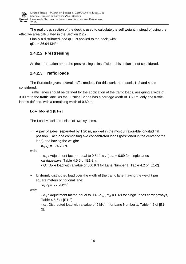
Load Model 2 [E1-2]
The Load Model 2 consists of a single axel load applied in the most unfavorable position,with a value of:
βQ Qak = 232 kNwith:
- βQ = αQ : Adjustment factor, equal to 0.844. αSL ( αSL = 0.69 for single lanes carriageways, Table 4.5.5 of [E1-3]).- Qak = 400kN
The details of the Load Model 2 are presented in the Figure 15.
PÁG.
17
MASTER THESIS – MASTER OF SCIENCE IN COMPUTATIONAL MECHANICS
STATICAL ANALYSIS OF NETWORK ARCH BRIDGES
UNIVERSITÄT STUTTGART – INSTITUT FÜR BAUSTATIK UND BAUDYNAMIK
2010
Figure 15. Load Model 2 [E1-2]
Load Model 4
The Load Model 4 represents the crowd loading, consisting on a uniform distributed loadequal to 5.0 kN/m2 [E1-2].
Loads on footpaths
For road bridges, an uniformly distributed load equal to 5kN/m2 should be applied in thefootpaths (Figure16) [E1-2].
Figure 16. Loads on footpaths [E1-2]
PÁG.
18

MASTER THESIS – MASTER OF SCIENCE IN COMPUTATIONAL MECHANICS
STATICAL ANALYSIS OF NETWORK ARCH BRIDGES
UNIVERSITÄT STUTTGART – INSTITUT FÜR BAUSTATIK UND BAUDYNAMIK
2010
2.4.2.4. Combination of Actions
Combining each Load Model (LM1, LM2 and LM4) with the loads on the footpaths, andconsidering the remaining areas, the following load configurations are obtained. As the analysis inthis thesis is made in 2D, only one arch will be analyzed. Hence, the loads that correspond to halfthe width of the bridge will be considered.
Load combination 1: LM1
The load combination that includes the Load Model 1 is called LM1. The details areshowed in the Figure 17.
Figure 17. Details of LM1 (Transversal and longitudinal)
PÁG.
19

MASTER THESIS – MASTER OF SCIENCE IN COMPUTATIONAL MECHANICS
STATICAL ANALYSIS OF NETWORK ARCH BRIDGES
UNIVERSITÄT STUTTGART – INSTITUT FÜR BAUSTATIK UND BAUDYNAMIK
2010
Uniformly distributed loads:
qLM1 = 5.00 kN/m2 . 1.30 m + 3.60 kN/m2 0.30 m + 5.20 kN/m2 . 1.50 m
qLM1 = 15.38 kN/m
Punctual Loads:
QLM1 = 174.7 kN . 0.50 = 87.35 kN
Load combination 2: LM2
The load combination that includes the Load Model 2 is called LM2. The details areshowed in the Figure 18.
Figure 18. Details of LM2 (Transversal and longitudinal)
PÁG.
20

MASTER THESIS – MASTER OF SCIENCE IN COMPUTATIONAL MECHANICS
STATICAL ANALYSIS OF NETWORK ARCH BRIDGES
UNIVERSITÄT STUTTGART – INSTITUT FÜR BAUSTATIK UND BAUDYNAMIK
2010
Uniformly distributed loads:
qLM2 = 5.00 kN/m2 . 1.30 m
qLM2 = 6.50 kN/m
Punctual Loads:
QLM2 = 232 kN . 0.50 = 116 kN
Load combination 4: LM4
The load combination that includes the Load Model 4 is called LM4. The details areshowed in the Figure 19.
Figure19. Details of LM4 (Transversal and longitudinal)
Uniformly distributed loads:
qLM2 = 5.00 kN/m2 . 3.10 m
qLM2 = 15.50 kN/m
PÁG.
21

MASTER THESIS – MASTER OF SCIENCE IN COMPUTATIONAL MECHANICS
STATICAL ANALYSIS OF NETWORK ARCH BRIDGES
UNIVERSITÄT STUTTGART – INSTITUT FÜR BAUSTATIK UND BAUDYNAMIK
2010
2.4.2.5. Load Cases
The different load cases are obtained combining the permanent loads and the traffic loadsaccording to the load combinations exposed in the Section 2.4.1. This is done for differentpositions of the punctual loads, in order to find the most unfavorable case.
For each position of the punctual loads, the load cases are:
Ed = 1.00 . Gfav + 1.35 . Gunfav + 1.50 . LM1 Ed = 1.00 . Gfav + 1.35 . Gunfav + 1.50 . LM2 Ed = 1.00 . Gfav + 1.35 . Gunfav + 1.50 . LM4
For every load case and each element, it must be verified that:
E dRd [E2-1]
The design value of resistance Rd is determined from the characteristic resistance of the
material divided by the partial factor on material strength γM:
Arch: Rd = 235000 KN/m2 / γM = 235000 KN/m2 / 1.10 = 213636 KN/m2 [E3-1.1]
Deck: Rd = 3200 KN/m2 / γM = 3200 KN/m2 / 1.50 = 2133 KN/m2 [E2-1]
Hangers: Rd = 500000 KN/m2 / γM = 500000 KN/m2 / 1.10 = 454545 KN/m2 [E3-1.1]
2.5Prestressing of the cables
The prestress force on the hangers is calculated in order to avoid the hangers to relax. Asa first step, the code was run with no consideration for the prestressing of the cables, consideringonly permanent loads.
It is found that under this conditions four hangers relaxed. As the element LINK10 do notwork under compression forces, the axial forces in the elements are equal to zero when thehangers have a negative axial deformation. Hence, the c force in each hanger is chosenmultiplying the value of the axial elastic strain by the elastic modulus.The axial elastic strains for the relaxed hangers are:
Hanger 18: 7.9e-5 Hanger 19: 3.8e-4Hanger 37: 9.09e-5Hanger 38: 3.4e-4
The resulting stresses are:Hanger 18: 16590 kN/m2
Hanger 19: 79800 kN/m2
Hanger 37: 19089 kN/m2
Hanger 38: 71400 kN/m2
PÁG.
22

MASTER THESIS – MASTER OF SCIENCE IN COMPUTATIONAL MECHANICS
STATICAL ANALYSIS OF NETWORK ARCH BRIDGES
UNIVERSITÄT STUTTGART – INSTITUT FÜR BAUSTATIK UND BAUDYNAMIK
2010
The stresses are applied as initial strains for the elements. The code is run one more timeunder this conditions. No hangers relax.
The code is also run for the case of partial load that is applying the traffic actions only inhalf of the span of the bridge. In this case also no hangers relax.
2.6 Results
The Lužnice Bridge is analyzed under two conditions: live load over the whole span andlive load over the right half of the span.
The tables with the results are included in Appendix B. The tables show next to each valuethe corresponding load case. For the case of LC1 and LC2, the punctual loads are applied indifferent positions along the span. The position of the punctual load is indicated by a number afterthe name of the load case. For example, LC1.12 means load case LC1, with the first punctual loadat 12.00 m from the left support in the case of even load, or 12.00 m from the center of the bridgein the case of partial load.
2.6.1. Deck
2.6.1.1. Even load
The Table B.1 shows the maximum and minimum values for the bending moments (M) andaxial forces (N) for the deck elements.
The first two pair of columns after the column “Element” show the values of the axial forceswith the corresponding load cases. As the axial forces in the deck are always positive, the columnof minimum should be ignored. The Figure 20 shows in a graphical format the maximum forces foreach element. The maximum value is 3543.5 kN and correspond to the element 2036, in thecenter of the span, and the load case 1.23, that is, the puntual load in the center of the span. Themaximum forces for all elements occur for the load case LC1. The axial forces are higher in thecenter of the span, decreasing as the element is closer to the supports. However, the values ofthe maximum axial forces are also important in the elements next to the supports. There arejumps between consecutive values, but they are in the order of 61 kN, that is less than the 2% ofthe average values.
The third pair of columns shows the maximum moments with the corresponding loadcases. The Figure 21 shows in a graphical format the maximum and minimum moments for eachelement. The maximum value is 872.00 kNm and corresponds to the element 2056, in the rightextreme of the deck, and the load case LC1.35 that is, the puntual load near the end of the span.The maximum bending moments in every element occur for LC1. The maximum moments arelower in the supports and in the center of the deck, and it have the highest value in the 1/5 and 4/5of the span.
The last pair of columns shows the minimum moments with the corresponding load cases.The Figure 21 shows in a graphical format the maximum and minimum moments for eachelement. The minimum value is -220.66 kNm and correspond to the element 4027, near the centerof the deck, and the load case 1.31 that is, the puntual load near the end of the span. The
PÁG.
23

MASTER THESIS – MASTER OF SCIENCE IN COMPUTATIONAL MECHANICS
STATICAL ANALYSIS OF NETWORK ARCH BRIDGES
UNIVERSITÄT STUTTGART – INSTITUT FÜR BAUSTATIK UND BAUDYNAMIK
2010
minimum moments in almost every element occur for LC1. The values that correspond to the loadcases LC2 and LC3 are positives and it should be ignored. The highest values are in the ¼ and ¾of the span.
The Table B.2 shows the maximum and minimum stresses for the deck elements. TheFigure 22 shows in a graphical format the maximum and minimum stresses for each element. Theminimum value for the stresses is -7288.32 kN/m2 and corresponds to the element 2056, in theright extreme of the deck, and the load case LC1.35 that is, the puntual load near the end of thespan. In the same way, the maximum value for the stresses is 15073.77 kN/m2 and correspondsto the element 2056 and the load case LC1.35. The minimum and maximum stresses for allelements occur for the load case LC1. The element next to the right support have a minimumstress for LC2, but its value is less than 0.1% of the highest value. The higher and lower valueoccur in 1/5 and 4/5 of the span respectively.The maximum stress is higher than the admisible value 2133 KN/m2; the minimum stress is lowerthan the admisible value -2133 KN/m2.The fact that the stresses are higher than the admissible values remarks the importance of theprestressing of the deck. As the prestressing was not considered in this thesis, this is expected.
Figure 20. Axial forces for the deck elements of the of the Lužnice bridge (Even load)
PÁG.
24

MASTER THESIS – MASTER OF SCIENCE IN COMPUTATIONAL MECHANICS
STATICAL ANALYSIS OF NETWORK ARCH BRIDGES
UNIVERSITÄT STUTTGART – INSTITUT FÜR BAUSTATIK UND BAUDYNAMIK
2010
Figure 21. Moments for the deck elements of the Lužnice bridge (Even load)
Figure 22. Stresses for the deck elements of the Lužnice bridge (Even load)
PÁG.
25

MASTER THESIS – MASTER OF SCIENCE IN COMPUTATIONAL MECHANICS
STATICAL ANALYSIS OF NETWORK ARCH BRIDGES
UNIVERSITÄT STUTTGART – INSTITUT FÜR BAUSTATIK UND BAUDYNAMIK
2010
2.6.1.2. Partial Load
The Table B.3 shows the maximum and minimum values for the bending moments (M) andaxial forces (N) for the deck elements.
The first two pair of columns after the column “Element” show the values of the axial forceswith the corresponding load cases. The Figure 23 shows in a graphical format the maximumforces for each element. As the axial forces in the deck are always positive, the column ofminimum should be ignored. The maximum value is 3292.62 kN and correspond to the element2065, in the right extreme the span, and the load case 1.10 that is, the puntual load in the ¾ of thespan. The maximum forces for all elements occur for the load case LC1. The axial forces arehigher as the element is closer to the right support, as the right half of the deck is the one loadedwith the live load. There are jumps between consecutive values, but their magnitude is of theorder of 50 kN, less than the 2% of the average values.
The third pair of columns shows the maximum bending moments with the correspondingload cases. The Figure 24 shows in a graphical format the maximum and minimum bendingmoments for each element. The maximum value is 1001.45 kNm and corresponds to the element2048 in the ¾ of the span, and the load case LC1.11, with the puntual load in the ¾ of the span.The maximum moments occur for the load cases LC1 and LC2. However the values for LC2 arenegative and should be ignored. The maximum moments have the highest value in the ¾ of thespan.
The last pair of columns shows the minimum bending moments with the correspondingload cases. The minimum value is -810.07 kNm and correspond to the element 4023, near the ¼of the span, and the load case 1.11, with the puntual load in the ¾ of the span. The minimummoments occur for LC1 and LC2. However the values for LC2 are positive and should be ignored.The maximum moments present the highest value in the ¼ of the span.
The Table B.4 shows the maximum and minimum stresses for the deck elements. TheFigure 25 shows in a graphical format the maximum and minimum stresses for each element. Theminimum value for the stresses is -9606.71 kN/m2 and correspond to the element 2048, in the ¾of the deck, and the load case LC1.11, with the puntual load in the ¾ of the span. In the sameway, the maximum value for the stresses is 16276.01 kN/m2 and corresponds to the element2048, and the load case LC1.11. The minimum and maximum stresses for all elements occur forthe load case LC1. The element next to the left support has a maximum stress for LC2, but itsvalue is less than 15% of the maximum value. The highest and lowest values occur in ¾ of thespan, with a minor peak at ¼ of the span.The maximum stress is higher than the admisible value 2133 KN/m2; the minimum stress is lowerthan the admisible value -2133 KN/m2. The fact that the stresses are higher than the admissible values remarks the importance of theprestressing of the deck. As the prestressing was not considered in this thesis, this is expected.
PÁG.
26

MASTER THESIS – MASTER OF SCIENCE IN COMPUTATIONAL MECHANICS
STATICAL ANALYSIS OF NETWORK ARCH BRIDGES
UNIVERSITÄT STUTTGART – INSTITUT FÜR BAUSTATIK UND BAUDYNAMIK
2010
Figure 23. Axial forces for the deck elements of the of the Lužnice bridge (Partial Load)
Figure 24. Moments for the deck elements of the Lužnice bridge (Partial Load)
PÁG.
27

MASTER THESIS – MASTER OF SCIENCE IN COMPUTATIONAL MECHANICS
STATICAL ANALYSIS OF NETWORK ARCH BRIDGES
UNIVERSITÄT STUTTGART – INSTITUT FÜR BAUSTATIK UND BAUDYNAMIK
2010
Figure 25. Stresses for the deck elements of the Lužnice bridge (Partial Load)
2.6.2. Arch
2.6.2.1. Even load
The Table B.5 shows the maximum and minimum values for the bending moments (M) andaxial forces (N) for the arch elements.
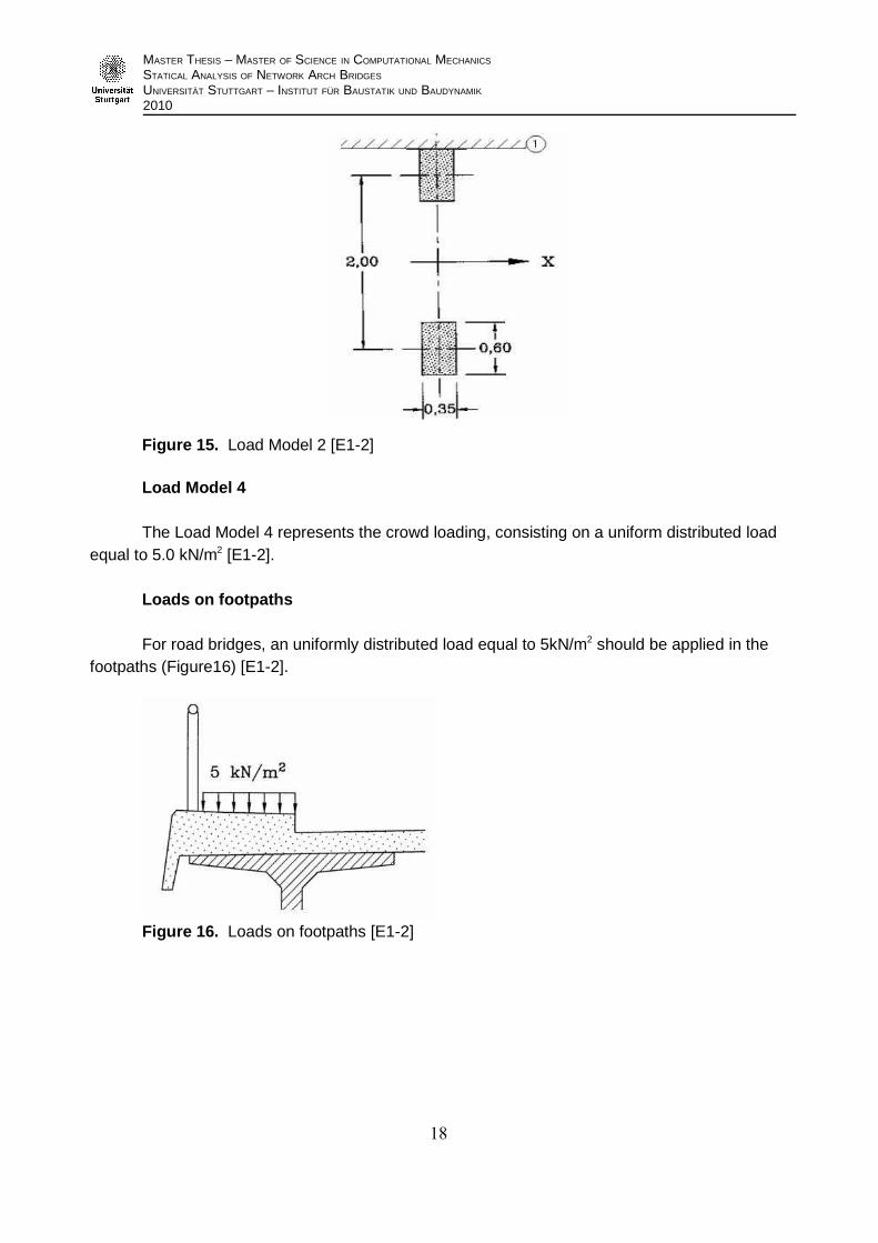
The first two pairs of columns after the column “Element” shows the values of the axialforces with the corresponding load cases. As the axial forces in the archs are always negative, thecolumn of maximum should be ignored. The Figure 26 shows in a graphical format the minimumforces for each element. The minimum value is –4025.23 kN and corresponds to the element4060, in the right extreme of the arch, and the load case 1.30, with the puntual load in the ¾ of thespan. The minimum forces for all elements occur for the load case LC1. The compression forcesin the center of the arch are significatly inferior than in the extremes.
The third pair of columns shows the maximum bending moments with the correspondingload cases. The Figure 27 shows in a graphical format the maximum and minimum moments foreach element. The maximum value is 136.79 kNm and corresponds to the element 4057 in theright extreme of the arch and the load case LC1.38, with the puntual load near the end of thespan. The maximum bending moment in almost every element occurs for LC1. In the last elementit occurs for LC3, however the value is less than 5% of the maximum.
The last pair of columns shows the minimum bending moments with the correspondingload cases. The minimum value is -109.35 kNm and corresponds to the element 4048, in the rightextreme of the arch, and the load case 1.12, with the puntual load in the ¼ of the span. Theminimum moment in almost every element occurs for LC1. However in the extreme the values
PÁG.
28
MASTER THESIS – MASTER OF SCIENCE IN COMPUTATIONAL MECHANICS
STATICAL ANALYSIS OF NETWORK ARCH BRIDGES
UNIVERSITÄT STUTTGART – INSTITUT FÜR BAUSTATIK UND BAUDYNAMIK
2010
correspond to the load case LC2 and are quite important, arriving to a 75% of the minimum. Theother minimum values that correspond to the LC2 are mostly positive values, hence should beignored.
The Table B.6 shows the maximum and minimum stresses for the arch elements. As thestresses are always negative the column of maximum stresses should be ignored. The Figure 28shows in a graphical format the maximum and minimum stresses for each element. The minimumvalue for the stresses is -175017.42 kN/m2 and correspond to the element 4057, in the rightextreme of the arch, and the load case 1.37, with the puntual load near the end of the span. Theminimum stresses for all elements ocur for the load case LC1. The minimum value is 82% of the minimum admisible stress (-213636 KN/m2 ).
Figure 26. Axial forces for the arch elements of the of the Lužnice bridge (Even load)
PÁG.
29

MASTER THESIS – MASTER OF SCIENCE IN COMPUTATIONAL MECHANICS
STATICAL ANALYSIS OF NETWORK ARCH BRIDGES
UNIVERSITÄT STUTTGART – INSTITUT FÜR BAUSTATIK UND BAUDYNAMIK
2010
Figure 27. Moments for the arch elements of the Lužnice bridge (Even load)
Figure 28. Stresses for the arch elements of the Lužnice bridge (Even load)
PÁG.
30

MASTER THESIS – MASTER OF SCIENCE IN COMPUTATIONAL MECHANICS
STATICAL ANALYSIS OF NETWORK ARCH BRIDGES
UNIVERSITÄT STUTTGART – INSTITUT FÜR BAUSTATIK UND BAUDYNAMIK
2010
2.6.1.2 Partial Load
The Table B.7 shows the maximum and minimum values for the bending moments (M) andaxial forces (N) for the arch elements.
The first two pairs of columns after the column “Element” show the values of the axialforces with the corresponding load cases. As the axial forces in the archs are always negative, thecolumn of maximum should be ignored. The Figure 29 shows in a graphical format the minimumforces for each element. The minimum value is –3772.30 kN and correspond to the element 4063,in the right extreme of the arch, and the load case 1.10, with the puntual load in the ¾ of the span.The minimum forces for all elements occur for the load case LC1. The compression forces in theright side of the arch are significatly higher, as the live load is only applied in the right half of thespan.
The third pair of columns shows the maximum bending moments with the correspondingload cases. The Figure 30 shows in a graphical format the maximum and minimum moments foreach element. The highest value is 185.72 kNm and correspond to the element 4038 in the 56%of the span, and the load case LC1.08, with the puntual load in the ¾ of the span. The maximumbending moment in the elements of the right half of the arch occurs for LC1. In the left half of thebridge, the maximum moments occurs for LC2. However they are positive or less than 25% of themaximum. In the right extreme the maximum occurs for LC3, but its value is less than 5% of themaximum.
The last pair of columns shows the minimum bending moments with the correspondingload cases. The Figure 30 shows in a graphical format the maximum and minimum moments foreach element. The minimum value is -165.05 kNm and correspond to the element 4012, in the lefthalf of the arch, and the load case 1.10, with the puntual load in the ¾ of the span. The minimummoments in the elements of the left side of the arch occurs for LC1. In the left side of the bridge,the minimum moments mostly occur for LC2. However they are positive or less than 40% of themaximum value.
The Table B.8 shows the maximum and minimum stresses for the arch elements. As thestresses are always negative the column of maximum stresses should be ignored. The Figure 31shows in a graphical format the maximum and minimum stresses for each element. The minimumvalue for the stresses is -177556.84 kN/m2 and correspond to the element 4039, in the center ofthe arch, and the load case 1.07, with the puntual load in the ¾ of the span. The minimumstresses for all elements occur for the load case LC1.
The minimum value is 83% of the minimum admisible stress (-213636 KN/m2 ).
PÁG.
31

MASTER THESIS – MASTER OF SCIENCE IN COMPUTATIONAL MECHANICS
STATICAL ANALYSIS OF NETWORK ARCH BRIDGES
UNIVERSITÄT STUTTGART – INSTITUT FÜR BAUSTATIK UND BAUDYNAMIK
2010
Figure 29. Axial forces for the arch elements of the of the Lužnice bridge (Partial load)
Figure 30. Moments for the arch elements of the Lužnice bridge (Partial load)
PÁG.
32

MASTER THESIS – MASTER OF SCIENCE IN COMPUTATIONAL MECHANICS
STATICAL ANALYSIS OF NETWORK ARCH BRIDGES
UNIVERSITÄT STUTTGART – INSTITUT FÜR BAUSTATIK UND BAUDYNAMIK
2010
Figure 31. Stresses for the arch elements of the Lužnice bridge (Partial load)
2.6.3. Hangers
2.6.3.1 Even load
The Table B.9 shows the maximum and minimum values for the stresses in the hangers.The hangers are ordered in two sets: one set is the mirrored equivalent of the other. The hangerswith a positive slope towards the right extreme of the bridge are referred as Set 1. The hangerswith a negative slope away from the right extreme of the bridge are referred as Set 2. Thenumbers for the hangers are assigned as it is shown in the Figure C.1 in the Appendix C.
In the Table, as the stresses are always positive, the column of minimum should beignored. The Figure 32 shows in a graphical format the maximum stresses in both sets. Thehighest value for the stresses is 194047.12 kN/m2 and corresponds to the element 2019, the lasthanger of the Set1, and the load case LC1.31, with the puntual load in the ¾ of the span. Themaximum stresses for most of the elements occur for the load case LC1. In the first hangers ofeach set the maximum stresses occur for LC3. However, the values in this hangers are inferiorthan the average value of the stresses. The highest values correspond to the last hangers of thesets, and they are significatly higher than the stresses in the rest of the hangers.
The maximum value is 42% of the maximum admisible stress (454545 KN/m2 ).
PÁG.
33

MASTER THESIS – MASTER OF SCIENCE IN COMPUTATIONAL MECHANICS
STATICAL ANALYSIS OF NETWORK ARCH BRIDGES
UNIVERSITÄT STUTTGART – INSTITUT FÜR BAUSTATIK UND BAUDYNAMIK
2010
Figure 32. Stresses for hangers of the Lužnice bridge (Full Load)
2.6.3.2 Partial Load
The Table B.10 shows the maximum and minimum values for the stresses in the hangers.The numbers for the hangers are assigned as it is shown in the Figure C.1 in the Appendix C.
In the Table, as the stresses are always positive, the column of minimum should beignored.
The Figure 33 shows in a graphical format the maximum stresses in both sets. The highestvalue for the stresses is 221057.17 kN/m2 and corresponds to the element 2019, the last hangerof the Set1, and the load case LC1.10, with the puntual load in the ¾ of the span. For this loadconfiguration the Set 1 is more solicitated than the Set2.
For the Set1 the maximum stresses for most of the elements occur for the load case LC1.In the first two hangers the maximum stresses occur for LC3. However, the values in this hangersare inferior than the average value of the stresses. For the Set2 the maximum stresses occur forthe load cases LC1, LC2 and LC3. The highest value in the last hanger occurs for LC2. This valueis 61% of the maximum value of the hangers of Set1.
The highest value is 48% of the maximum admisible stress (454545 KN/m2 ).
PÁG.
34

MASTER THESIS – MASTER OF SCIENCE IN COMPUTATIONAL MECHANICS
STATICAL ANALYSIS OF NETWORK ARCH BRIDGES
UNIVERSITÄT STUTTGART – INSTITUT FÜR BAUSTATIK UND BAUDYNAMIK
2010
Figure 33. Stresses for hangers of the Lužnice bridge (Partial Load)
2.7 Conclusions
The maximum and minimum stresses in the elements occur mainly for the load case LC1.Even if for some elements the stresses correspond to another load case, those values aresignificantly smaller compared with the values of the most loaded elements.
In the case of partial loading of the deck, in the hangers that belong to the Set 2, themaximum stresses occurred for LC2. However for this case the Set1 is significantly more stressedthan the Set2. Hence, the highest values correspond to the load case LC1.
For these reason, the study of the bridge will be done only for the load case LC1.On the other hand, comparing the cases of even and partial loading, the absolute values of
the maximum and minimum stresses are quite similar, slightly higher in the second case. But, ithas to be considered that under asymmetric loading the benefits of network arch bridges overother types of bridges become more evident. This can be clearly seen in the Figure 22 that showsthe stresses in the deck for even loads. While the distributed load in the deck is always even, thepunctual load for LC1 change position. In this way, the maximum stress in the center of the deck,that corresponds to a central position of the punctual load (symmetric load), is smaller than themaximum stress at 1/5 of the span, that corresponds to a punctual load at 1/5 of the span(asymmetric load). The stresses in the deck under asymmetric loads are higher than undersymmetric loads. Also, under partial loading, the hangers are more susceptible to relax.
Hence, the study will be done for partial loading of the span.
PÁG.
35

MASTER THESIS – MASTER OF SCIENCE IN COMPUTATIONAL MECHANICS
STATICAL ANALYSIS OF NETWORK ARCH BRIDGES
UNIVERSITÄT STUTTGART – INSTITUT FÜR BAUSTATIK UND BAUDYNAMIK
2010
PÁG.
36

MASTER THESIS – MASTER OF SCIENCE IN COMPUTATIONAL MECHANICS
STATICAL ANALYSIS OF NETWORK ARCH BRIDGES
UNIVERSITÄT STUTTGART – INSTITUT FÜR BAUSTATIK UND BAUDYNAMIK
2010
Chapter 3
Study of parameters
This Chapter constitutes the main part of this thesis. Different parameters are studied in
order to find how they influence the structural behavior and, therefore, the solicitations on the
elements of the bridge.
The parameters chosen for this study are:
− Hangers arrangement. Section 3.1
− Arch shape. Section 3.2
− Number of hangers. Section 3.3
− Rise of the arch. Section 3.4
An optimal arrangement is characterised by the following attributes [GST]:
− economic/inexpensive.
− fast/easy to build.
− functional,aesthetic,ecological...
This attributes are mainly influenced by the minimum and maximum internal forces. Hence,
for this work the following atributes are chosen:
− Maximum and minimum bending moments.
− Maximum and minimum axial forces.
− Maximum and minimum stresses.
The maximum bending moments are not analyzed for the hangers, as this elements are
tension-only. For the arch and the deck, the moments with the maximum absolute values are
considered.
The minimum axial forces are considered for the hangers, in order to study the posibility of
relaxation.
Over 973 bridges are modelled for this study. For each model, the avobe mentioned
parameters are stored in matrices for its analysis. Aditional parameters are also analyzed, as the
number of relaxed hangers, and the load cases and coordinates or elements corresponding to the
maximum solicitations. The values that are considered useful for the interpretations of the
structural behavior of the bridge are presented in this work.
PÁG.
37

MASTER THESIS – MASTER OF SCIENCE IN COMPUTATIONAL MECHANICS
STATICAL ANALYSIS OF NETWORK ARCH BRIDGES
UNIVERSITÄT STUTTGART – INSTITUT FÜR BAUSTATIK UND BAUDYNAMIK
2010
3.1. Hanger arrangement
Two types of arrangements are considered. In the Section 3.1.1. an arrangement based on
the linear variation of the slope of the hangers is presented [TNA]. In the Section 3.1.2. the radial
arrangement, proposed by Brunn and Schanack [BSC] is analyzed.
Each hanger arrangement is studied for a circular arch shape, following the
recomendations in [TNA]. The radio of the circular arch is adopted in order to mantain the span
and the maximum height of the original arch.
3.1.1. Linear variation of the slopes
This arrangement is based on a constant angle change between adjacent hangers [TNA].
The upper nodes of the hangers are placed equidistantly along the arch. The slope of each
hanger increase lineary from an start angle, according to the function:
=0n−1
Where ϕ0 is the initial angle and ∆ϕ is the angle increment between hangers. The value n is
the number of the hanger. Hence the variables used to described this arrangement are the initial
angle and the angle increment.
Figure 34. Arrangement of the hangers based on the linear variation of the slopes
For the present study 340 bridges are calculated, with a start angle from 65° to 84°
and with an angle increment from 0.0° to 3.4°. The study is done for a circular arch shape. The
numbers for the hangers are assigned as it is shown in the Figure C.1 in the Appendix C.
PÁG.
38

MASTER THESIS – MASTER OF SCIENCE IN COMPUTATIONAL MECHANICS
STATICAL ANALYSIS OF NETWORK ARCH BRIDGES
UNIVERSITÄT STUTTGART – INSTITUT FÜR BAUSTATIK UND BAUDYNAMIK
2010
3.1.1.1. Results
The results are shown in the following diagrams. Every ordinate corresponds to one value
of each bridge.
3.1.1.1.1. Bending moments in the deck
The Figure 35 shows the absolute values for maximum bending moments in the deck for
each bridge. The highest value presents for a bridge with ϕ0= 84° - ∆ϕ = 0.0°. This configuration is
shown in the Figure 36. The bending moments decrease as the initial angle decreases and as the
angle increment increases, until a minimum value for a bridge with ϕ0= 70° - ∆ϕ = 3.2°. This
configuration is shown in the Figure 37.
Figure 35. Maximum bending moments in the deck (Linear variation of the slopes)
Figure 36. Hanger arrangement for ϕ0= 84° - ∆ϕ = 0.0°
PÁG.
39
MASTER THESIS – MASTER OF SCIENCE IN COMPUTATIONAL MECHANICS
STATICAL ANALYSIS OF NETWORK ARCH BRIDGES
UNIVERSITÄT STUTTGART – INSTITUT FÜR BAUSTATIK UND BAUDYNAMIK
2010
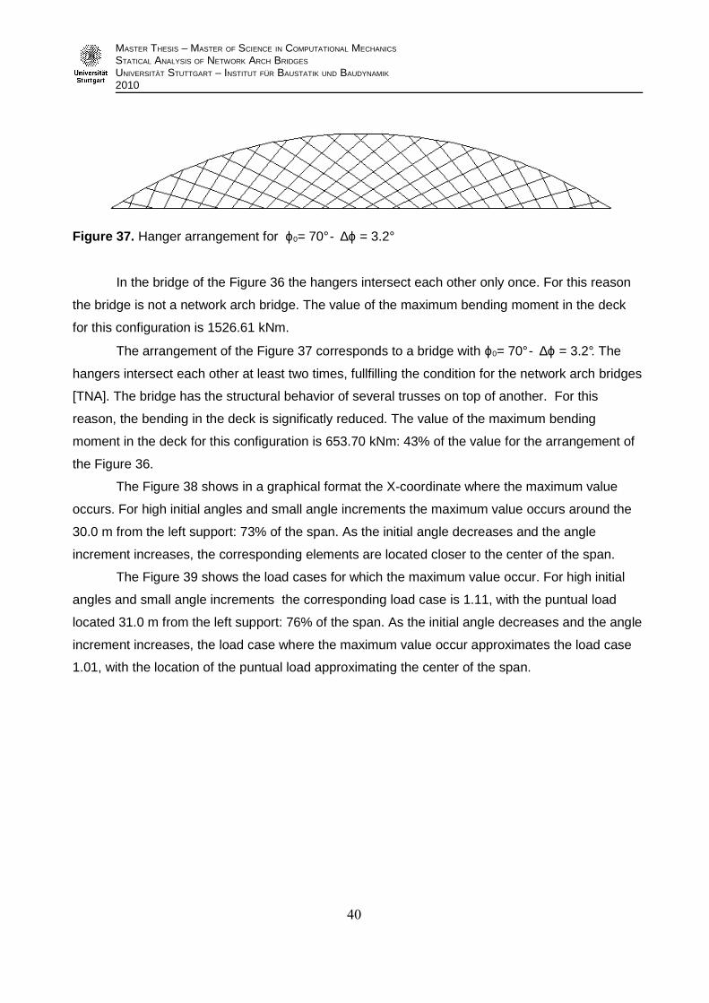
Figure 37. Hanger arrangement for ϕ0= 70° - ∆ϕ = 3.2°
In the bridge of the Figure 36 the hangers intersect each other only once. For this reason
the bridge is not a network arch bridge. The value of the maximum bending moment in the deck
for this configuration is 1526.61 kNm.
The arrangement of the Figure 37 corresponds to a bridge with ϕ0= 70° - ∆ϕ = 3.2°. The
hangers intersect each other at least two times, fullfilling the condition for the network arch bridges
[TNA]. The bridge has the structural behavior of several trusses on top of another. For this
reason, the bending in the deck is significatly reduced. The value of the maximum bending
moment in the deck for this configuration is 653.70 kNm: 43% of the value for the arrangement of
the Figure 36.
The Figure 38 shows in a graphical format the X-coordinate where the maximum value
occurs. For high initial angles and small angle increments the maximum value occurs around the
30.0 m from the left support: 73% of the span. As the initial angle decreases and the angle
increment increases, the corresponding elements are located closer to the center of the span.
The Figure 39 shows the load cases for which the maximum value occur. For high initial
angles and small angle increments the corresponding load case is 1.11, with the puntual load
located 31.0 m from the left support: 76% of the span. As the initial angle decreases and the angle
increment increases, the load case where the maximum value occur approximates the load case
1.01, with the location of the puntual load approximating the center of the span.
PÁG.
40

MASTER THESIS – MASTER OF SCIENCE IN COMPUTATIONAL MECHANICS
STATICAL ANALYSIS OF NETWORK ARCH BRIDGES
UNIVERSITÄT STUTTGART – INSTITUT FÜR BAUSTATIK UND BAUDYNAMIK
2010
Figure 38. Corresponding X-coordinates for the maximum bending moments in the deck
(Linear variation of the slopes)
Figure 39. Corresponding load cases for the maximum bending moments in the deck
(Linear variation of the slopes)
PÁG.
41

MASTER THESIS – MASTER OF SCIENCE IN COMPUTATIONAL MECHANICS
STATICAL ANALYSIS OF NETWORK ARCH BRIDGES
UNIVERSITÄT STUTTGART – INSTITUT FÜR BAUSTATIK UND BAUDYNAMIK
2010
3.1.1.1.2. Axial forces in the deck
The Figure 40 shows the values for maximum axial forces in the deck for each bridge. The
highest value presents for a bridge with ϕ0= 65° - ∆ϕ = 3.4°. This configuration is shown in the
Figure 41. The axial forces decrease as the initial angle increases and as the angle increment
decreases, until a minimum value for a bridge with ϕ0= 84° - ∆ϕ = 0.0°. This configuration is shown
in the Figure 36.
In the arrengement of the Figure 41 the hangers intersect each other at least two times,
fullfilling the condition for the network arch bridges [TNA]. The bridge has the structural behavior
of several trusses on top of another. The value of the maximum axial force in the deck for this
configuration is 3294.64 kN.
The bridge shown on the Figure 36 is not a network arch bridge, as the hangers just
intersect each other once. The value of the maximum axial force in the deck for this configuration
is 2844.75 kN: 86% of the highest axial force.
Figure 40. Maximum axial forces in the deck (Linear variation of the slopes)
PÁG.
42

MASTER THESIS – MASTER OF SCIENCE IN COMPUTATIONAL MECHANICS
STATICAL ANALYSIS OF NETWORK ARCH BRIDGES
UNIVERSITÄT STUTTGART – INSTITUT FÜR BAUSTATIK UND BAUDYNAMIK
2010
Figure 41. Hanger arrangement for ϕ0= 65° - ∆ϕ = 3.4°
The Figure 42 shows in a graphical format the X-coordinates where the maximum values
occur. For all bridges, the maximum value ocurrs mostly near 35.0 m from the left support (85% of
the span). However, as the angle increment increases and the initial angle decreases, the
corresponding coordinate approaches the right support.
The Figure 43 shows the load cases for which the maximum values occur. For high initial
angles and small angle increments the corresponding load case is 1.01, with the puntual load
located in the center of the span. As the initial angle decrease and as the angle increment
increase, the load case where the maximum value occur approximates the load case 1.12. That
is, the location of the puntual load approximates to the 32 m from the left support: the 78% of the
span.
Figure 42 . Corresponding X-coordinates for the maximum axial forces in the deck (Linear
variation of the slopes)
PÁG.
43

MASTER THESIS – MASTER OF SCIENCE IN COMPUTATIONAL MECHANICS
STATICAL ANALYSIS OF NETWORK ARCH BRIDGES
UNIVERSITÄT STUTTGART – INSTITUT FÜR BAUSTATIK UND BAUDYNAMIK
2010
Figure 43. Corresponding load cases for the maximum bending moments in the deck
(Linear variation of the slopes )
3.1.1.1.3. Stresses in the deck
The Figure 44 shows the values for maximum stresses in the deck for each bridge. The
highest value presents for a bridge with ϕ0= 84° - ∆ϕ = 0.0°. This configuration is shown in the
Figure 36. The stresses decrease as the initial angle decreases and as the angle increment
increases, until a minimum value for a bridge with ϕ0= 70° - ∆ϕ = 3.2°. This configuration is shown
in the Figure 37.
In the bridge of the Figure 36 the hangers intersect each other only once. For this reason
the bridge is not a network arch bridge. The value of the maximum stress in the deck for this
configuration is 22806.53 kN/m2.
The arrangement of the Figure 37 corresponds to a bridge with ϕ0= 70° - ∆ϕ = 3.2°. The
hangers intersect each other at least two times, fullfilling the condition for the network arch bridges
[TNA]. The bridge has the structural behavior of several trusses on top of another. For this
reason, the stress in the deck is significatly reduce in comparison with the arrangement of the
Figure 36. The value of the maximum stress in the deck for this configuration is 11461.62 kN/m2: a
reduction of 50%.
PÁG.
44

MASTER THESIS – MASTER OF SCIENCE IN COMPUTATIONAL MECHANICS
STATICAL ANALYSIS OF NETWORK ARCH BRIDGES
UNIVERSITÄT STUTTGART – INSTITUT FÜR BAUSTATIK UND BAUDYNAMIK
2010
Figure 44. Maximum stresses in the deck (Linear variation of the slopes)
The figure 45 shows in a graphical format the X-coordinate where the maximum values
occur. For high initial angles and small angle increments the maximum values occur near the 30.0
m from the left support: 75% of the span. As the initial angle decreases and the angle increment
increases, the corresponding coordinate is closer to the center of the span.
The Figure 46 shows the load cases for which the maximum values occur. For high initial
angles and small angle increments the corresponding load case is 1.11, with the puntual load
located 31 m from the left support: 76% of the span. As the initial angle decreases and the angle
increment increases, the load case where the maximum value occurs approaches the load case
1.01, with the location of the puntual load approximating the center of the span.
.
PÁG.
45

MASTER THESIS – MASTER OF SCIENCE IN COMPUTATIONAL MECHANICS
STATICAL ANALYSIS OF NETWORK ARCH BRIDGES
UNIVERSITÄT STUTTGART – INSTITUT FÜR BAUSTATIK UND BAUDYNAMIK
2010
Figure 45. Corresponding X-coordinate for the maximum stresses in the deck (Linear
variation of the slopes)
Figure 46. Corresponding load cases for the maximum stresses in the deck (Linear
variation of the slopes)
PÁG.
46

MASTER THESIS – MASTER OF SCIENCE IN COMPUTATIONAL MECHANICS
STATICAL ANALYSIS OF NETWORK ARCH BRIDGES
UNIVERSITÄT STUTTGART – INSTITUT FÜR BAUSTATIK UND BAUDYNAMIK
2010
3.1.1.1.4. Bending moments in the arch
The Figure 44 shows the absolute values for maximum bending moments in the arch for
each bridge. The highest value presents for a bridge with ϕ0= 84° - ∆ϕ = 0.0°. This configuration is
shown in the Figure 36. The stresses decrease as the initial angle decreases and as the angle
increment increases, until a minimum value for a bridge with ϕ0= 70° - ∆ϕ = 3.2°.
In the bridge of the Figure 36 the hangers intersect each other only once. For this reason
the bridge is not a network arch bridge. The value of the maximum bending moment in the arch for
this configuration is 197.89 kNm.
The arrangement of the Figure 37 corresponds to a bridge with ϕ0= 70° - ∆ϕ = 3.2°. The
hangers intersect each other at least two times, fullfilling the condition for the network arch bridges
[TNA]. The bridge has the structural behavior of several trusses on top of another. For this
reason, the stress in the deck is significatly reduce. The value of the maximum stress in the deck
for this configuration is 75.28 kNm: 38% of the value for the arrangement of the Figure 36..
The Figure 48 shows in a graphical format the X-coordinates where the maximum values
occur. The maximum bending moments occur mostly 9.0 m from the left support (22% of the
span), except for small initial angles and high angle increments, in which the corresponding
coordinates approache the right support.
Figure 47. Maximum bending moments in the arch (Linear variation of the slopes)
PÁG.
47

MASTER THESIS – MASTER OF SCIENCE IN COMPUTATIONAL MECHANICS
STATICAL ANALYSIS OF NETWORK ARCH BRIDGES
UNIVERSITÄT STUTTGART – INSTITUT FÜR BAUSTATIK UND BAUDYNAMIK
2010
Figure 48. Corresponding X-coordinate for the maximum bending moments in the arch
(Linear variation of the slopes)
3.1.1.1.5. Axial forces in the arch
The Figure 49 shows the values for maximum axial compression forces in the arch for
each bridge. The highest compression force presents for a bridge with ϕ0= 65° - ∆ϕ = 3.4°. This
configuration is shown in the Figure 41. The values decrease as the initial angle increases and as
the angle increment decreases, until a minimum value for a bridge with ϕ0= 84° - ∆ϕ = 0.0°. This
configuration is shown in the Figure 36.
In the arrengement of the Figure 41 the hangers intersect each other at least two times,
fullfilling the condition for the network arch bridges [TNA]. The bridge has the structural behavior
of several trusses on top of another. The value of the maximum compression force in the arch for
this configuration is -4001.34 kN.
The bridge of the Figure 36 is not a network arch bridge, as the hangers intersect each
other only once. The value of the maximum compression force in the arch for this configuration is
-3285.81 kN: 82% of the value for the arrengement of the Figure 41.
PÁG.
48

MASTER THESIS – MASTER OF SCIENCE IN COMPUTATIONAL MECHANICS
STATICAL ANALYSIS OF NETWORK ARCH BRIDGES
UNIVERSITÄT STUTTGART – INSTITUT FÜR BAUSTATIK UND BAUDYNAMIK
2010
Figure 49. Maximum axial compression forces in the arch (Linear variation of the slopes)
The Figure 50 shows in a graphical format the X-coordinate where the maximum values
occur. For high initial angles and small angle increments the maximum compression force is
located in the right extreme of the arch. As the initial angle decrease and the angle increment
increase, the location of the maximum value approximates the center of the span.
The Figure 51 shows the load cases for which the maximum values occur. In the Figure it
can be seen a “central peak”. In the points with ϕ0= 84° - ∆ϕ = 0.0° and ϕ0= 65° - ∆ϕ = 3.4° the
load case where the maximum value occurs is around 1.01, with the puntual load in the center of
the span. As the variables approach the “central peak”, the corresponding load case
approximates 1.10, with the puntual load located 30.0 m from the left support: 75% of the span.
PÁG.
49

MASTER THESIS – MASTER OF SCIENCE IN COMPUTATIONAL MECHANICS
STATICAL ANALYSIS OF NETWORK ARCH BRIDGES
UNIVERSITÄT STUTTGART – INSTITUT FÜR BAUSTATIK UND BAUDYNAMIK
2010
Figure 50 . Corresponding X-coordinate for the maximum axial compression forces in the
arch (Linear variation of the slopes)
Figure 51 . Corresponding load cases for the maximum axial compression forces in the
arch (Linear variation of the slopes)
PÁG.
50

MASTER THESIS – MASTER OF SCIENCE IN COMPUTATIONAL MECHANICS
STATICAL ANALYSIS OF NETWORK ARCH BRIDGES
UNIVERSITÄT STUTTGART – INSTITUT FÜR BAUSTATIK UND BAUDYNAMIK
2010
3.1.1.1.6. Stresses in the arch
The Figure 52 shows the values for maximum negative stresses in the arch for each
bridge. The highest value presents for a bridge with ϕ0= 70° - ∆ϕ = 0.0°. This configuration is
shown in the Figure 53. The negative stress decrease as the initial angle decreases and as the
angle increment increases, until a minimum value for a bridge with ϕ0= 73° - ∆ϕ = 3.0°. This
configuration is shown in the Figure 54.
In the arrangement of the Figure 53, the hangers intersect each other two times, fullfilling
the condition for the network arch bridges [TNA]. The bridge has the structural behavior of two
trusses on top of another. The value of the maximum negative stress in the arch for this
configuration is -189623.73 kN/m2.
In the arrangement of the Figure 54, the hangers intersect each other more than two
times, fullfilling the condition for the network arch bridges [TNA]. The bridge has the structural
behavior of six trusses on top of another. The value of the maximum negative stress in the arch
for this configuration is -140129.41 kN/m2, of 74% the value for configuration in the Figure 53.
Figure 52. Maximum stresses in the arch (Linear variation of the slopes)
PÁG.
51

MASTER THESIS – MASTER OF SCIENCE IN COMPUTATIONAL MECHANICS
STATICAL ANALYSIS OF NETWORK ARCH BRIDGES
UNIVERSITÄT STUTTGART – INSTITUT FÜR BAUSTATIK UND BAUDYNAMIK
2010
Figure 53. Hanger arrangement for ϕ0= 70° - ∆ϕ = 0.0°
Figure 54. Hanger arrangement for ϕ0= 73° - ∆ϕ = 3.0°
The Figure 55 shows in a graphical format the X-coordinate where the maximum value
occur. For values of ∆ϕ less than 2.8°, the maximum values occur near the l eft support. For angle
increments bigger than 3.0°, the corresponding elem ents are located next to the right support.
Figure 55 . Corresponding X-coordinate for the maximum stresses in the arch (Linear
variation of the slopes)
PÁG.
52

MASTER THESIS – MASTER OF SCIENCE IN COMPUTATIONAL MECHANICS
STATICAL ANALYSIS OF NETWORK ARCH BRIDGES
UNIVERSITÄT STUTTGART – INSTITUT FÜR BAUSTATIK UND BAUDYNAMIK
2010
3.1.1.1.7. Stresses in the hangers
The Figure 56 shows the values for maximum stresses in the hangers for each bridge.The
highest value presents for a bridge with ϕ0= 65° - ∆ϕ = 3.4°. This configuration is shown in the
Figure 41. The values decrease as the initial angle increases and as the angle increment
decreases, until a minimum value for a bridge with ϕ0= 84° - ∆ϕ = 0.0°. This configuration is shown
in the Figure 36.
In the arrengement of the Figure 41 the hangers intersect each other at least two times,
fullfilling the condition for the network arch bridges [TNA]. The bridge has the structural behavior
of several trusses on top of another. The value of the maximum stress in the hangers for this
configuration is 176697.25 kN/m2.
The bridge of the Figure 36 is not a network arch bridge, as the hangers intersect each
other only once. The value of the maximum stress in the hangers for this configuration is
106608.15 kN/m2: 60% of the value for the configuration in the Figure 53.
Figure 56. Maximum stresses in the hangers (Linear variation of the slopes)
PÁG.
53

MASTER THESIS – MASTER OF SCIENCE IN COMPUTATIONAL MECHANICS
STATICAL ANALYSIS OF NETWORK ARCH BRIDGES
UNIVERSITÄT STUTTGART – INSTITUT FÜR BAUSTATIK UND BAUDYNAMIK
2010
3.1.1.1.8. Relaxed hangers
The Figure 57 shows the number of relaxed hangers for each bridge. The prestressing of
the hangers was not considered. In the Figure, it can be noticed an area where there are no
relaxed hangers. For values of the initial angle smaller than 73° and angle increments smaller
than 2.2°, the structure presents relaxed hangers.
The relaxed hangers are located in the extremes of the bridge, next to the supports.
The relaxed hangers are:
− One relaxed hanger: 3001
− Two relaxed hangers: 3001; 3038
The elements 3001 is the first hanger of the Set 1. The element 3038 is the last hanger of
the Set 2.
The Figure 58 shows a hanger arrangement with ϕ0= 65° - ∆ϕ = 0.0°. This configuration
presents two relaxed hangers in the extremes. A configuration with no relaxed hangers is shown
in the Figure 41, with ϕ0= 65° - ∆ϕ = 3.4°.
Figure 57. Number of relaxed hangers (Linear variation of the slopes)
PÁG.
54

MASTER THESIS – MASTER OF SCIENCE IN COMPUTATIONAL MECHANICS
STATICAL ANALYSIS OF NETWORK ARCH BRIDGES
UNIVERSITÄT STUTTGART – INSTITUT FÜR BAUSTATIK UND BAUDYNAMIK
2010
Figure 58. Hanger arrangement for ϕ0= 65° - ∆ϕ = 0.0°
3.1.1.2. Conclusions
The Figure 59 shows the number of times the hangers intersect each other in each bridge.
The bridge behaves as a network arch bridge if the number of intersections is at least two.
Figure 59. Number of times the hangers intersect each other in each bridge
For small angle increments and big initial angles, the numer of intersections is equal to 1,
hence the corresponding bridges are not network arch. As the angle increment increases and the
initial angle decreases, the number of intersections increase.
If in a structure the hangers intersect each other two times, the bridge have the structural
behavior of two trusses on top of another, giving less bending in the arch and the deck. This effect
PÁG.
55

MASTER THESIS – MASTER OF SCIENCE IN COMPUTATIONAL MECHANICS
STATICAL ANALYSIS OF NETWORK ARCH BRIDGES
UNIVERSITÄT STUTTGART – INSTITUT FÜR BAUSTATIK UND BAUDYNAMIK
2010
will be greater if the hangers intersect several times, as the structural behavior corresponds to
several trusses on top of another. Hence, as the numer of intersections increases ,the bending
moments in the arch and deck decreases.
The bending moments in the deck correspond to those in the arch, and in both cases the
highest values occur in the bridges that do not behave like network arch bridges. The lowest
values are obtained for small initial angles and big angle increments, which corresponds to the
bridges in which the hangers intersect each other several times. The reduction is important: 40%
of the highest values in both cases.
The axial forces in the deck also correspond to the axial forces in the arch. In this case the
lowest values are obtained for the hanger arrangement with ϕ0= 84° - ∆ϕ = 0.0°, that do not
behaves as network arch bridges. However, in the graphics for the deck and the arch it can be
observed that the maximum and the minimum values are only isolated peaks. Outside this two
values, the variation of the axial forces is not important. As an example two points are taken. In
the deck, for a hanger arrangement with ϕ0= 70 - ∆ϕ = 2.8°, the axial force is 3015.80 kN. For an
hanger arrangement with ϕ0= 80 - ∆ϕ = 1.0°, the axial force is 2967.14 kN : the reduct ion is of only
2%. The same occur for the arch.
From this we can say that the hanger arrangement has an important influence on the
values of the bending moments in the deck and arch, while the variation in the axial forces due to
the arrangement it is not significant.
Hence, it is expectable that the form of the graphic for maximum stresses in the arch and
in the deck corresponds to the one obtained for the moments. The lowest values are obtained for
small initial angles and big increment angles, which corresponds to bridges in which the hangers
intersect each other several times.
The maximum stresses in the hangers are obtained for the bridges in which the hangers
intersect each other several times. As the number of intersections decreases, the stresses
decrease. For a number of intersections inferior to 3 the increment is not significant, less than 5%.
However, for a higher number of intersections the stresses in the hangers increase very fast,
arriving to an increment of 36% for 6 intersections and 61% for 10 intersections.
In the arch and the hangers the stresses are lower than the admissible values. The
fact that the stresses in the deck are higher than the admissible values remarks the importance of
the prestressing of the deck. As the prestressing was not considered in this thesis, it was expected
than the admissible stress are exceeded.
According to the Figure 57, the relaxation of the hangers occur for small initial angles and
small angle increments.
PÁG.
56

MASTER THESIS – MASTER OF SCIENCE IN COMPUTATIONAL MECHANICS
STATICAL ANALYSIS OF NETWORK ARCH BRIDGES
UNIVERSITÄT STUTTGART – INSTITUT FÜR BAUSTATIK UND BAUDYNAMIK
2010
The Figure 41 and 58 show configurations with ϕ0= 65° - ∆ϕ = 3.4° and ϕ0= 65° - ∆ϕ =
0.0° respectively. While the first case presents no relaxation, the second case presents two
relaxed hangers. The configuration of Figure 58 shows steeper hangers than in the case of Figure
41, which leads to more relaxed hangers. This confirms what can be found in [TNA] : “Too steep
hangers lead to too much relaxation of hangers”.
Also steeper hangers lead to bigger bending moments and deflections. The Figures 60 and
61 show the deformation for the load case 1.01 with ϕ0= 65° - ∆ϕ = 0.0° and ϕ0= 65° - ∆ϕ = 3.4°
respectively. In the first Figure the arch move to the left, increasing deflection and bending
moments, with the presence of relaxed hangers in the extremes. On the other hand the
deformation for the second configuration shows a better distribution of the forces, with smaller
deflections and no relaxed hangers.
Therefore, while small initial angles and high angle increments results in low stresses in
arch and deck but important stresses in the hangers, high initial angles and small angle
increments results in low stresses in the hangers but important stresses in arch and deck.
Moreover, small initial angles and small angle increments cause relaxed hangers. Hence, a
hanger arrangements with high initial angles and high angle increments provides the best results.
Figure 60. Deformations for hanger arrangements with ϕ0= 65° - ∆ϕ = 0.0°
Figure 61. Deformations for hanger arrangements with ϕ0= 65° - ∆ϕ = 3.4°
PÁG.
57

MASTER THESIS – MASTER OF SCIENCE IN COMPUTATIONAL MECHANICS
STATICAL ANALYSIS OF NETWORK ARCH BRIDGES
UNIVERSITÄT STUTTGART – INSTITUT FÜR BAUSTATIK UND BAUDYNAMIK
2010
3.1.2. Radial arrangement
Brunn and Schanack proposed this arrangement in their diploma thesis [BSC].
The loads are distributed uniformly acting in the radial direction of the arch. This decreases
the bending moments in an arch with circular shape. Also the axial forces in the hangers result
smaller.
If all the hangers have the same axial force, it could be considered that the resulting forces
of the hangers are directed along the connecting lines of their intersections, as shown in the
Figure 62.
However, due to the presence of moving loads, the axial forces in the hangers are not the
same. Nonetheless, this still could be considered as a good approximation.
Figure 62. Radial arrangement [BSC]
The upper nodes of the hangers are placed equidistantly along the arch [TNA]. The
variable for this arrangement is the angle with which the hangers cross each other. For this study,
the variable adopted is the angle between radius and hanger at the first crossing of the hangers
below the arch, as shown in the Figure 63.
Figure 63. Radial arrangement. The adopted variable is the angle marked as grey [BSC]
For the present study 115 bridges are calculated, with a cross angle from 0° to 57°. The
study is done for a circular arch shape. The number of element for the hangers is assigned as
shown in the Figure C.2 in the Appendix C.
PÁG.
58

MASTER THESIS – MASTER OF SCIENCE IN COMPUTATIONAL MECHANICS
STATICAL ANALYSIS OF NETWORK ARCH BRIDGES
UNIVERSITÄT STUTTGART – INSTITUT FÜR BAUSTATIK UND BAUDYNAMIK
2010
3.1.2.1. Results
The results are shown in the following diagrams. Every ordinate corresponds to one value
of each bridge.
3.1.2.1.1. Bending moments in the deck
The Figure 64 shows the absolute values for maximum bending moments in the deck for
each bridge. If we see the Figure, we notice that the values decrease from a cross angle equal to
0° until a minimum between 40° and 50°. From 50° to 57° the bending moments increase
significatly.
Figure 64. Maximum bending moments in the deck (Radial arrangement)
The Figure 65 shows an arrangement with a cross angle equal to 45° that corresponds to
the minimum bending moments.
Figure 65. Radial arrangement. Cross angle = 45°
PÁG.
59

MASTER THESIS – MASTER OF SCIENCE IN COMPUTATIONAL MECHANICS
STATICAL ANALYSIS OF NETWORK ARCH BRIDGES
UNIVERSITÄT STUTTGART – INSTITUT FÜR BAUSTATIK UND BAUDYNAMIK
2010
In the arrangement of Figure 65 the hangers intersect each other several times. This fulfill
the condition for the network arch bridges. For this reason the bending moments in the deck are
significantly reduce. The maximum bending moment for this arrangement is 656.50 kNm. That is
36% of the value for the “spoked wheel arrangement” with the cross angle equal to 0°: 1836.17
kNm and in the same order of the best value for the arrangements with linear variation of the
slopes: 653.70 kNm.
The Figure 66 shows in a graphical format the X-coordinates where the maximum values
occur. For cross angles smaller than 30° the corres ponding element is between 30.0 m and 33.0
m from the left support that is between 73% and 80% of the span. As the cross angle is increased,
the maximum value presents closer to the center of the span. For a cross angle equal to 55° the
maximum value occurs 21.48 m from the left support (52% of the span).
Figure 66. Corresponding X-coordinates for the maximum bending moments in the deck
(Radial arrangement)
The Figure 67 shows the load cases for which the maximum values occur. If the cross
angle is smaller than 34° the corresponding load ca se approaches 1.13, with the punctual load
located 34.0 m from the left support: 83% of the span. For cross angles bigger than 45° the
corresponding load case approximates 1.02, with the punctual load situated near the center of the
span.
PÁG.
60

MASTER THESIS – MASTER OF SCIENCE IN COMPUTATIONAL MECHANICS
STATICAL ANALYSIS OF NETWORK ARCH BRIDGES
UNIVERSITÄT STUTTGART – INSTITUT FÜR BAUSTATIK UND BAUDYNAMIK
2010
Figure 67. Corresponding load cases for the maximum bending moments in the deck
(Radial arrangement)
3.1.2.1.2. Axial Forces in the deck
The Figure 68 shows the values for maximum axial forces in the deck for each bridge. The
lowest values appear as the arrangement approaches to a “spoked wheel” arrangement, that is
when the cross angle is equal to 0°. As the cross a ngle increases, the maximum axial forces are
higher. However, the variation is not important for cross angles smaller than 50°. For angles bigger
than 50° the axial forces increase significantly.
The axial force for an arrangement with a cross angle equal to 0° is 2925.13 kN. For a
cross angle equal to 50° the axial force is 3084.93 kN: 1.05 times the previous value.
For a cross angle equal to 57° the maximum axial fo rce is 3468.89 kN: 1.19 times the
value for a cross angle equal to 0°.
The Figure 69 shows in a graphical format the X-coordinate where the maximum values
occur. For small values of the cross angle the maximum values occur near the center of the span.
As the cross angle is increased, the maximum value presents closer to the right support. For a
cross angle equal to 55° the maximum value occurs n ext to the right support.
PÁG.
61

MASTER THESIS – MASTER OF SCIENCE IN COMPUTATIONAL MECHANICS
STATICAL ANALYSIS OF NETWORK ARCH BRIDGES
UNIVERSITÄT STUTTGART – INSTITUT FÜR BAUSTATIK UND BAUDYNAMIK
2010
Figure 68. Maximum axial forces in the deck (Radial arrangement)
Figure 69. Corresponding X-coordinates for the maximum axial forces in the deck (Radial
arrangement)
PÁG.
62

MASTER THESIS – MASTER OF SCIENCE IN COMPUTATIONAL MECHANICS
STATICAL ANALYSIS OF NETWORK ARCH BRIDGES
UNIVERSITÄT STUTTGART – INSTITUT FÜR BAUSTATIK UND BAUDYNAMIK
2010
The Figure 70 shows the load cases for which the maximum values occur. When the cross
angle is small the corresponding load case is around 1.01, with the punctual load near the center
of the span. As the cross angle increases, the position of the punctual load that correspond to the
maximum value approaches the right support. For a cross angle equal to 55° the maximum value
occurs for the load case 1.13 that corresponds to the punctual load 6.00 m from the right support.
Figure 70. Corresponding load cases for the maximum axial forces in the deck (Radial
arrangement)
3.1.2.1.3. Stresses in the deck
The Figure 71 shows the values for maximum stresses in the deck for each bridge. If we
see the figure, we notice that values decrease from a cross angle equal to 0° until a minimum
between 40° and 50°. From 50° to 57° the stresses i ncrease significantly.
The figure 65 shows an arrangement with a cross angle equal to 45° that corresponds to
the minimum values for the stresses. In this arrangement the hangers intersect each other several
times. This fulfill the condition for network arch bridges. For this reason the stress in the deck is
significantly reduce. The value of the stress for this arrangement is 11520.15 kN/m2. That is 43%
of the value for the “spoked wheel arrangement” with a cross angle equal to 0°: 26714.00 kN/m 2.
and it is in the same order of the best value for the arrangements with linear variation of the
slopes: 11461.62 kN/m2.
PÁG.
63

MASTER THESIS – MASTER OF SCIENCE IN COMPUTATIONAL MECHANICS
STATICAL ANALYSIS OF NETWORK ARCH BRIDGES
UNIVERSITÄT STUTTGART – INSTITUT FÜR BAUSTATIK UND BAUDYNAMIK
2010
Figure 71. Maximum stresses in the deck (Radial arrangement)
The Figure 72 shows in a graphical format X-coordinate where the maximum values occur.
For cross angles smaller than 30° the corresponding element is between 30.0 m and 33.0 m from
the left support that is between 73% and 80% of the span. As the cross angle is increased, the
maximum value presents closer to the center of the span. For a cross angle equal to 55° the
maximum value occurs 21.48 m from the left support (52% of the span).
The Figure 73 shows the load cases for which the maximum values occur. If the cross
angle is smaller than 34° the corresponding load ca se approximates 1.13, with the punctual load
34.00 m from the left support. For cross angles bigger than 40° the corresponding load case
approaches 1.03, with the punctual load situated near the center of the span.
PÁG.
64

MASTER THESIS – MASTER OF SCIENCE IN COMPUTATIONAL MECHANICS
STATICAL ANALYSIS OF NETWORK ARCH BRIDGES
UNIVERSITÄT STUTTGART – INSTITUT FÜR BAUSTATIK UND BAUDYNAMIK
2010
Figure 72. Corresponding X-coordinates for the maximum stresses in the deck (Radial
arrangement)
Figure 73. Corresponding load cases for the maximum stresses in the deck (Radial
arrangement)
PÁG.
65
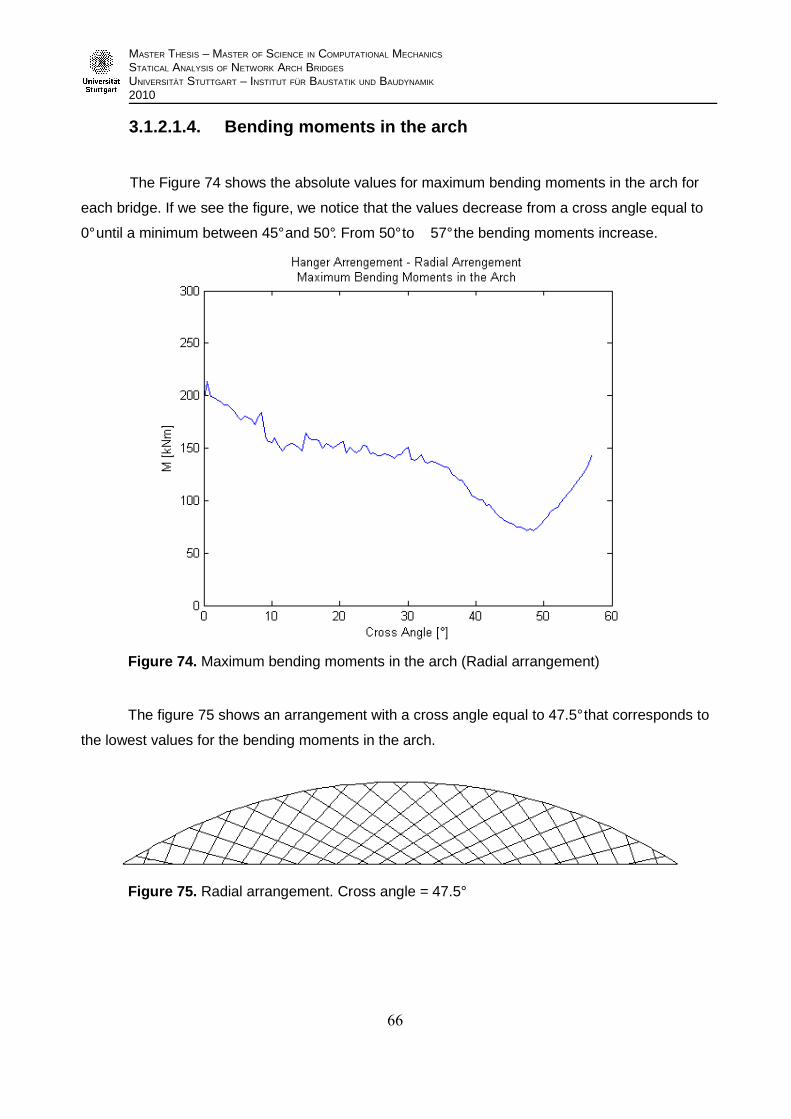
MASTER THESIS – MASTER OF SCIENCE IN COMPUTATIONAL MECHANICS
STATICAL ANALYSIS OF NETWORK ARCH BRIDGES
UNIVERSITÄT STUTTGART – INSTITUT FÜR BAUSTATIK UND BAUDYNAMIK
2010
3.1.2.1.4. Bending moments in the arch
The Figure 74 shows the absolute values for maximum bending moments in the arch for
each bridge. If we see the figure, we notice that the values decrease from a cross angle equal to
0° until a minimum between 45° and 50°. From 50° to 57° the bending moments increase.
Figure 74. Maximum bending moments in the arch (Radial arrangement)
The figure 75 shows an arrangement with a cross angle equal to 47.5° that corresponds to
the lowest values for the bending moments in the arch.
Figure 75. Radial arrangement. Cross angle = 47.5°
PÁG.
66

MASTER THESIS – MASTER OF SCIENCE IN COMPUTATIONAL MECHANICS
STATICAL ANALYSIS OF NETWORK ARCH BRIDGES
UNIVERSITÄT STUTTGART – INSTITUT FÜR BAUSTATIK UND BAUDYNAMIK
2010
In the arrangement of Figure 75 the hangers intersect each other several times. This fulfill
the condition the network arch bridges. For this reason the bending moments in the arch are
significantly reduce. The value of the bending moment for this arrangement is 71.02 kNm. That is
37% of the value for the “spoked wheel arrangement” with the cross angle equal to 0°: 194.48
kNm and 95% of the best value for the arrangements with linear variation of the slopes: 75.28
kNm.
The figure 76 shows in a graphical format the X-coordinate where the maximum values
occur. The maximum values occur less than 10.00 m from the left or right support. That is,
between the 0% and 25% of the span or between the 75% and 100%. Exceptions are the hanger
arrangements with cross angles between 42° and 50°.
Figure 76. Corresponding X-coordinates for the maximum bending moments in the arch
(Radial arrangement)
The Figure 77 shows in a graphical format the number of the load cases for which the
maximum values occur. The maximum values occur mostly for the load cases between 1.04 and
1.16. This corresponds to a position of the punctual load between 25.00 m and 37.00 m from the
left support that is 61% and 90% of the span.
PÁG.
67

MASTER THESIS – MASTER OF SCIENCE IN COMPUTATIONAL MECHANICS
STATICAL ANALYSIS OF NETWORK ARCH BRIDGES
UNIVERSITÄT STUTTGART – INSTITUT FÜR BAUSTATIK UND BAUDYNAMIK
2010
Figure 77. Corresponding load cases for the maximum bending moments in the arch
(Radial arrangement)
3.1.2.1.5. Axial forces in the arch
The Figure 78 shows the values for maximum axial compression forces in the arch for
each bridge. If we see the figure, we notice that the lowest values for the compression forces
correspond to the “spoked wheel arrangement” shown in the Figure 79. From this point the
compression forces increase as the cross angle increases.
For this arrangement the hangers do not intersect each other. For this reason the bridge is
not a network arch bridge. The corresponding maximum axial force is -3019.53 kN. That is 71% of
the maximum value, that corresponds to a cross angle of 57°: -4236.86 kN; and 92% of the best
value for the arrangements with linear variation of the slopes: -3285.81 kN.
PÁG.
68

MASTER THESIS – MASTER OF SCIENCE IN COMPUTATIONAL MECHANICS
STATICAL ANALYSIS OF NETWORK ARCH BRIDGES
UNIVERSITÄT STUTTGART – INSTITUT FÜR BAUSTATIK UND BAUDYNAMIK
2010
Figure 78. Maximum axial compression forces in the arch (Radial arrangement)
Figure 79. Radial arrangement. Cross angle = 0°
The figure 80 shows in a graphical format the X-coordinates where the maximum values
occur. For a cross hanger smaller than 40° the maxi mum compression forces occurs in the
extremes of the arch. As the cross angle is increased, the maximum value presents closer to the
center of the span. For a cross angle of 57° the ma ximum compression force occurs at a distance
of 25 m from the left support: 61% of the span.
PÁG.
69

MASTER THESIS – MASTER OF SCIENCE IN COMPUTATIONAL MECHANICS
STATICAL ANALYSIS OF NETWORK ARCH BRIDGES
UNIVERSITÄT STUTTGART – INSTITUT FÜR BAUSTATIK UND BAUDYNAMIK
2010
Figure 80. Corresponding X-coordinates for the maximum axial compression forces in the
arch (Radial arrangement)
The Figure 81 shows the load cases for which the maximum values occur. For cross
angles smaller than 35°, the position of the punctu al load that corresponds to the maximum axial
compression force approaches the ¾ of the span, as the angle is increase. For a cross angle
equal to 0° the load case is 1.01, with the punctua l load in the center of the span. For a cross
angle of 35° the corresponding load case is 1.10, w ith the punctual load 30.00 m from the left
support: 73% of the span.
For cross angles bigger than 35°, the corresponding position of the punctual load
approaches the middle of the span as the angle increases. For a cross angle of 57° the
corresponding load case is 1.03, with the punctual load 24.00 m from the left support: 58% of the
span.
PÁG.
70

MASTER THESIS – MASTER OF SCIENCE IN COMPUTATIONAL MECHANICS
STATICAL ANALYSIS OF NETWORK ARCH BRIDGES
UNIVERSITÄT STUTTGART – INSTITUT FÜR BAUSTATIK UND BAUDYNAMIK
2010
Figure 81. Corresponding load cases for the maximum axial compression forces in the
arch (Radial arrangement)
3.1.2.1.6. Stresses in the arch
The Figure 82 shows the values for maximum negative stresses in the arch for each
bridge. If we see the figure, we notice that the values decrease from a cross angle equal to 0° until
a minimum between 40° and 50°. From 50° to 57° the stresses increase significantly.
The figure 65 shows an arrangement with a cross angle equal to 45° that corresponds to
the lowest values for the stresses.
In the arrangement of Figure 65 the hangers intersect each other several times. Hence,
the bridge has the structural behavior of several trusses on top of another. This fulfill the condition
for network arch bridges. For this reason the negative stress in the arch is reduced. The value of
the maximum negative stress for this arrangement is -142108.92 kN/m2. That is 81% of the value
for the “spoked wheel arrangement”: -173534.36 kN/m2; and in the same order of the best value
for the arrangements with linear variation of the slopes: -140129.41 kN/m2.
PÁG.
71

MASTER THESIS – MASTER OF SCIENCE IN COMPUTATIONAL MECHANICS
STATICAL ANALYSIS OF NETWORK ARCH BRIDGES
UNIVERSITÄT STUTTGART – INSTITUT FÜR BAUSTATIK UND BAUDYNAMIK
2010
The Figure 83 shows in a graphical format the X-coordinates where the maximum values
occur. The maximum values occur less than 10.00 m from the left or right support. That is,
between the 0% and 25% of the span or between the 75% and 100%.
The Figure 84 shows in a graphical format the number of the load cases for which the
maximum values occur. The maximum values occur mostly for the load cases between 1.06 and
1.14. This corresponds to a position of the punctual load between 27.00 m and 35.00 m from the
left support that is 66% and 85% of the span.
Figure 82. Maximum stresses in the arch (Radial arrangement)
PÁG.
72

MASTER THESIS – MASTER OF SCIENCE IN COMPUTATIONAL MECHANICS
STATICAL ANALYSIS OF NETWORK ARCH BRIDGES
UNIVERSITÄT STUTTGART – INSTITUT FÜR BAUSTATIK UND BAUDYNAMIK
2010
Figure 83. Corresponding X-coordinates for the maximum stresses in the arch (Radial
arrangement)
Figure 84. Corresponding load cases for the maximum stresses in the arch (Radial
arrangement)
PÁG.
73

MASTER THESIS – MASTER OF SCIENCE IN COMPUTATIONAL MECHANICS
STATICAL ANALYSIS OF NETWORK ARCH BRIDGES
UNIVERSITÄT STUTTGART – INSTITUT FÜR BAUSTATIK UND BAUDYNAMIK
2010
3.1.2.1.7. Stresses in the hangers
The Figure 85 shows the values for maximum stresses in the hangers for each bridge. The
minimum stress corresponds to a cross angle equal to 0°. However, for angle smaller than 25° the
stresses do not increase significantly. The maximum stress for an angle of 0° is 87588.89 kN/m 2,
while for an angle of an angle of 21° is 104875.21 kN/m2: 1.20 times the previous value.
For angles bigger than 25° the increment of the str esses becomes more important. The
stress for an angle of 50° is 153067.13 kN/m 2: 1.75 times the stress for a cross angle of 0°. Th e
stress for an angle of 57° is 212251.66 kN/m 2: 2.42 times the stress for a cross angle of 0°.
The values for the arrangements with linear variation of the slopes are bigger than the
values for the radial arrangement. The best value for the first case is 106608.15 kN/m2, 1.22 times
the best value for radial arrangement.
Figure 85. Maximum stresses in the hangers (Radial arrangement)
The Figure 86 shows in a graphical format the number of the element where the maximum
values occur. The maximum stresses always correspond to an element between 3009 and 3035,
that is, the hangers located at a distance bigger than 8 .00 m from the supports: between the 20%
and 80% of the span. For cross angles bigger than 35°, as the angle increase the hanger with the
maximum stress approaches the center of the span.
PÁG.
74
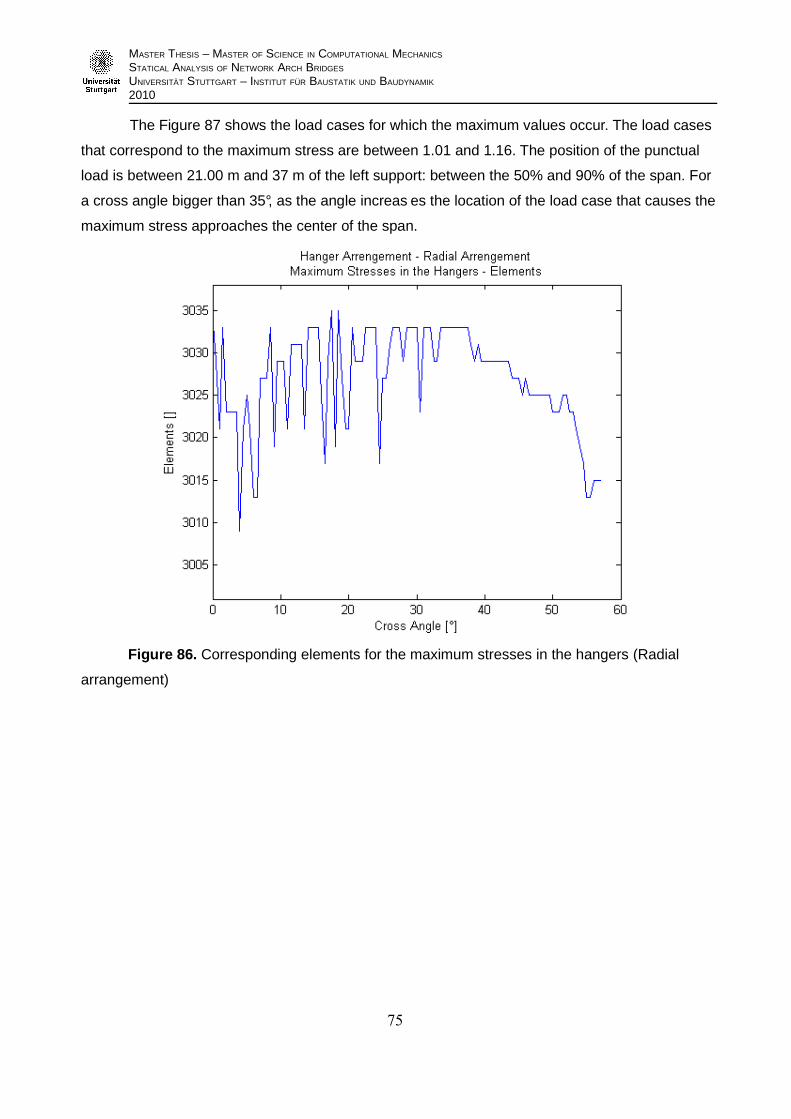
MASTER THESIS – MASTER OF SCIENCE IN COMPUTATIONAL MECHANICS
STATICAL ANALYSIS OF NETWORK ARCH BRIDGES
UNIVERSITÄT STUTTGART – INSTITUT FÜR BAUSTATIK UND BAUDYNAMIK
2010
The Figure 87 shows the load cases for which the maximum values occur. The load cases
that correspond to the maximum stress are between 1.01 and 1.16. The position of the punctual
load is between 21.00 m and 37 m of the left support: between the 50% and 90% of the span. For
a cross angle bigger than 35°, as the angle increas es the location of the load case that causes the
maximum stress approaches the center of the span.
Figure 86. Corresponding elements for the maximum stresses in the hangers (Radial
arrangement)
PÁG.
75

MASTER THESIS – MASTER OF SCIENCE IN COMPUTATIONAL MECHANICS
STATICAL ANALYSIS OF NETWORK ARCH BRIDGES
UNIVERSITÄT STUTTGART – INSTITUT FÜR BAUSTATIK UND BAUDYNAMIK
2010
Figure 87. Corresponding load cases for the maximum stresses in the hangers (Radial
arrangement)
3.1.2.1.8. Relaxed hangers
The Figure 88 shows the number of relaxed hangers for each bridge. There are no relaxed
hangers for most of the hanger arrangements. The exceptions are the configurations that
correspond to cross angles equal to 1° and 9°, with one relaxed hanger, and to an angle equal to
3.5°, with three relaxed hangers.
For the radial arrangement, the relaxed hangers are located in the center of the bridge.
None of this configurations corresponds to network arch bridges.
The relaxed hangers are:
− Cross angle = 1°: 3019
− Cross angle = 3.5°: 3018, 3021, 3022.
− Cross angle = 9°: 3017.
The maximum number of relaxed hangers correspond to the load case 1.06. The position
of the punctual load is 27.00 m from the left support that is 66% of the span.
PÁG.
76

MASTER THESIS – MASTER OF SCIENCE IN COMPUTATIONAL MECHANICS
STATICAL ANALYSIS OF NETWORK ARCH BRIDGES
UNIVERSITÄT STUTTGART – INSTITUT FÜR BAUSTATIK UND BAUDYNAMIK
2010
Figure 88. Number of relaxed hangers (Radial arrangement)
3.1.2.2. Conclusions
A network arch bridge configuration is obtained when the hangers intersect each other at
least two times. This is achieved when the cross angle is higher than 15°.
The minimum bending moments in the deck are obtained for cross angles between 40°
and 50°. For angles bigger than 50° or smaller than 40° the increment of the moments is
important.
On the other hand, for angles smaller than 50° the influence of the cross angle over the
axial forces is the deck is very small, around 5%. Even for angles bigger than 50° the influence is
not significant: less than 15%.
For this reason the form of the graphic obtained for the stresses in deck is quite similar to
the one obtained for the bending moments. As in the case of the hanger arrangement based in the
linear variation of the slopes, the configuration of the hangers has important an influence on the
values of the bending moments in the deck, while the variation of the axial forces due to the
arrangement is not significant.
PÁG.
77

MASTER THESIS – MASTER OF SCIENCE IN COMPUTATIONAL MECHANICS
STATICAL ANALYSIS OF NETWORK ARCH BRIDGES
UNIVERSITÄT STUTTGART – INSTITUT FÜR BAUSTATIK UND BAUDYNAMIK
2010
Comparing the results for this arrangement with the results for the hanger arrangement
based in the linear variation of the slopes we find similar results, with slightly higher values for the
second case. While for the radial arrangement the stresses in the deck are between 11520.15 kN/
m2 and 26714.00 kN/m2 , for the arrangement based in the linear variation of the slopes the values
are between 11461.62 kN/m2 and 22806.53 kN/m2.
The minimum bending moments in the arch are obtained for cross angles between 45° and
50°. For angles bigger than 50° or smaller than 45° the increase of the moments is important. The
influence of the cross angle over the axial forces in the arch is more significant than in the deck.
Comparing the results in the arch for this arrangement with the results for the hanger
arrangement based in the linear variation of the slopes we do not find any improvement. The
stresses are of the same order in both cases.
In the deck the elements where the maximum stress occur are in the center of the span,
while in the arch the elements located in the extremes quarters are the ones that support the
highest stresses. The hangers near the center of the span present the higher stresses.
In the arch and hangers the stresses are lower than the admissible values. The fact that
the stresses in the deck are higher than the admissible values remarks the importance of the
prestressing of the deck. As the prestressing was not considered in this thesis, it is expected than
the admissible stresses are exceeded.
The smallest stresses in the hangers are obtained for small cross angles, approaching the
“spoked wheel configuration”. For bigger angles the values increase significantly. Here we find an
improvement: the values for the radial arrangement are 82% smaller than the results for the
hanger arrangement based in the linear variation of the slopes:
Only three configurations show relaxed hangers. This hanger arrangements do not
correspond to network arch bridges, as the hangers do not intersect each other at least two times.
The bridges that fulfill this condition have no relaxed hangers.
PÁG.
78

MASTER THESIS – MASTER OF SCIENCE IN COMPUTATIONAL MECHANICS
STATICAL ANALYSIS OF NETWORK ARCH BRIDGES
UNIVERSITÄT STUTTGART – INSTITUT FÜR BAUSTATIK UND BAUDYNAMIK
2010
3.2. Shape of the arch
In order to examine the influence of the shape of the arch over the structural behavior of
the bridge two principal arch shapes are chosen: the parabolic arch, and the circular arch.
In addition, it is considered the possibility of the combination of this two shapes. A
parabolic shape is adopted in the extremes of the arch, and a circular shape in the center. The
circular part of the arch in this case has a radius bigger than the one obtained for a fully circular
arch. In the point where the circular arch meets the parabolic arch, the tangent line has the same
slope.
The variables use to describe this configuration are the radio of the circular part of the arch
RRel, and the distance from where the parabolic shape begins, long1. The radio Rrel is expressed
as a percentage of the radius for a fully circular arch, with Rrel > 1.0. The distance long1 is
expressed as a percentage of the span, with long1 ≤ 0.5. This variables are shown in the Figure
89.
Figure 89. Variables used to described the shape of the arch
A hanger arrangement that corresponds to a linear variation of the slopes is used for this
examination, with an initial angle of 70° and an an gle increment of 1.0°. The bridge configuration
is shown in figure 90.
Figure 90. Hanger arrangement for ϕ0= 70° - ∆ϕ = 1.0°
PÁG.
79

MASTER THESIS – MASTER OF SCIENCE IN COMPUTATIONAL MECHANICS
STATICAL ANALYSIS OF NETWORK ARCH BRIDGES
UNIVERSITÄT STUTTGART – INSTITUT FÜR BAUSTATIK UND BAUDYNAMIK
2010
The results obtained for this bridge are:
− Maximum bending moment in the deck: 971.30 kNm
− Maximum axial force in the deck: 3068.27 kN
− Maximum Stress in the deck: 15884.76 kN/m2
− Maximum bending moment in the arch: -188.50 kNm
− Maximum axial force in the arch: -3448.22 kN
− Maximum stress in the arch: -176040.98 kN/m2
− Maximum stress in the hangers: 124854.89 kN/m2
− Number of relaxed hangers: 2
For the present study 400 bridges are calculated, with a radius Rrel from 1.1 to 3.0, and a
distance long1 from 0.05 to 0.5. The numbers assigned to the hanger elements are the same as
for the hanger arrangement based on the linear variation of the slope, as shown in the Figure C.1
in the Appendix C.
3.2.1. Results
The results are shown in the following diagrams. Every ordinate corresponds to one value
of each bridge.
3.2.1.1. Bending moments in the deck
The Figure 91 shows the absolute values for maximum bending moments in the deck for
each bridge. The maximum stress increase as Rrel increases and long1 decreases until a
maximum value at Rrel = 3 and long1 = 0.05. This configuration is shown in the Figure 92.
For the bridge shown in the Figure 92 the maximum axial force is 4025.09 kNm , 4.10
times the value obtain for a circular arch shape.
The stress for a parabolic arch is represented in the graphic for the points with distance
long1 = 0.5. The Figure 93 shows an example for this configuration. The maximum bending
moment for a parabolic arch is 971.81 kNm, approximately the same value as for a circular arch
shape.
PÁG.
80

MASTER THESIS – MASTER OF SCIENCE IN COMPUTATIONAL MECHANICS
STATICAL ANALYSIS OF NETWORK ARCH BRIDGES
UNIVERSITÄT STUTTGART – INSTITUT FÜR BAUSTATIK UND BAUDYNAMIK
2010
Figure 91. Maximum bending moments in the deck (Shape of the arch)
Figure 92. Arch shape: Rrel=3.0 ; long1 = 0.05
Figure 93. Arch shape: Rrel=1.0 ; long1 = 0.50
The Figure 94 shows the X-coordinates where maximum values occur. For long1 smaller
than 0.35, the maximum bending moment presents 4.00 m from the left support (10% of the
span). For long1 bigger than 0.35, it occurs around the 25.00 m from the left support, that is 61%
of the span. For circular arches the corresponding coordinate is 27.80 m from the left support
(70% of the span).
PÁG.
81

MASTER THESIS – MASTER OF SCIENCE IN COMPUTATIONAL MECHANICS
STATICAL ANALYSIS OF NETWORK ARCH BRIDGES
UNIVERSITÄT STUTTGART – INSTITUT FÜR BAUSTATIK UND BAUDYNAMIK
2010
Figure 94. Corresponding X-coordinates for the maximum bending moments in the deck
(Shape of the arch)
The Figure 95 shows the load cases for which the maximum values occur. For long1
smaller than 0.30, the position of the punctual load is around 28.00 m form the left support (load
case 1.07), that is 68% of the span. For values of long1 between 0.30 and 0.45 the position of the
punctual load that causes the maximum bending moment is near the center of the span.
For parabolic (long1=0.5) and circular arches the corresponding load cases are
around 1.10, with the punctual load 31.00 m from the left support (76% of the span).
PÁG.
82

MASTER THESIS – MASTER OF SCIENCE IN COMPUTATIONAL MECHANICS
STATICAL ANALYSIS OF NETWORK ARCH BRIDGES
UNIVERSITÄT STUTTGART – INSTITUT FÜR BAUSTATIK UND BAUDYNAMIK
2010
Figure 95. Corresponding load cases for the maximum bending moments in the deck
(Shape of the arch)
3.2.1.2. Axial forces in the deck
The Figure 96 shows the values for maximum axial forces in the deck for each bridge.
Axial forces decrease as Rrel increases and long1 decreases, until a minimum value at Rrel = 3 and
long1 = 0.05. This configuration is shown in the Figure 92.
The bending moment for a parabolic arch is represented in the graphic by the points with
distance long1 = 0.5. The Figure 93 shows this configuration. The maximum axial force for a
parabolic arch is 3141.16 kNm, 1.02 times the value for a circular arch shape.
For the bridge with Rrel = 3 and long1 = 0.05 the maximum axial force is 2452,48 kN, 80%
of the value obtained for a circular arch shape.
PÁG.
83

MASTER THESIS – MASTER OF SCIENCE IN COMPUTATIONAL MECHANICS
STATICAL ANALYSIS OF NETWORK ARCH BRIDGES
UNIVERSITÄT STUTTGART – INSTITUT FÜR BAUSTATIK UND BAUDYNAMIK
2010
Figure 96. Maximum axial forces in the deck (Shape of the arch)
The figure 97 shows in a graphical format the X-coordinates where the maximum values
occur. For long1 between 0.15 and 0.35 and Rrel higher than 1.4 the maximum axial forces occur
approximately in the middle of the span. In the rest of the graphic the maximum values present
35.00 m from the left support: 85% of the span.
The Figure 98 shows the load cases for which the maximum values occur. For long1
smaller than 0.35, the corresponding load case is around 1.02: the location of the punctual load is
in the center of the span. For long1 bigger than 0.35, the position of the punctual load is around
30.00 m form the left support (load case 1.09): 73% of the span. For small values of Rrel the
position of the punctual load that causes the maximum axial force is less centered in the span,
approaching the right support.
PÁG.
84

MASTER THESIS – MASTER OF SCIENCE IN COMPUTATIONAL MECHANICS
STATICAL ANALYSIS OF NETWORK ARCH BRIDGES
UNIVERSITÄT STUTTGART – INSTITUT FÜR BAUSTATIK UND BAUDYNAMIK
2010
Figure 97. Corresponding X-coordinates for the maximum axial forces in the deck (Shape
of the arch)
Figure 98. Corresponding load cases for the maximum axial forces in the deck (Shape of
the arch)
PÁG.
85

MASTER THESIS – MASTER OF SCIENCE IN COMPUTATIONAL MECHANICS
STATICAL ANALYSIS OF NETWORK ARCH BRIDGES
UNIVERSITÄT STUTTGART – INSTITUT FÜR BAUSTATIK UND BAUDYNAMIK
2010
3.2.1.3. Stresses in the deck
The Figure 99 shows the values for maximum stresses in the deck for each bridge. The
maximum stress increase as Rrel increases and long1 decreases until a maximum value at Rrel = 3
and long1 = 0.05. This configuration is shown in the Figure 92. For this bridge the maximum axial
force is 54397,71 kN/m2 , 3.41 times the value obtained for a circular arch shape.
The stress for a parabolic arch is represented in the graphic for the points with distance
long1 = 0.5. The Figure 93 shows this configuration. The maximum stress for a parabolic arch is
15963,19 kN/m2, approximately the same value that for a circular arch shape.
Figure 99. Maximum stresses in the deck (Shape of the arch)
The Figure 100 shows the X-coordinates where maximum values occur. For long1 smaller
than 0.25, the maximum stress presents 7.00 m from the left support (10% of the span). For
long1 bigger than 0.25, it occurs around 25.00 m from the left support: 61% of the span. For
circular arches the corresponding coordinate is 27.80 m from the left support (70% of the span).
PÁG.
86

MASTER THESIS – MASTER OF SCIENCE IN COMPUTATIONAL MECHANICS
STATICAL ANALYSIS OF NETWORK ARCH BRIDGES
UNIVERSITÄT STUTTGART – INSTITUT FÜR BAUSTATIK UND BAUDYNAMIK
2010
Figure 100. Corresponding X-coordinates for the maximum stresses in the deck (Shape of
the arch)
The Figure 101 shows the load cases for which the maximum values occur. For long1
smaller than 0.25, the position of the punctual load is around 28.00 m form the left support (load
case 1.07): 68% of the span. For values of long1 between 0.25 and 0.45 the position of the
punctual load that causes the maximum axial force is near the center of the span.
For parabolic (long1=0.5) and circular arches the corresponding load cases are around
1.12, with the punctual load 33.00 m from the left support (80% of the span).
PÁG.
87

MASTER THESIS – MASTER OF SCIENCE IN COMPUTATIONAL MECHANICS
STATICAL ANALYSIS OF NETWORK ARCH BRIDGES
UNIVERSITÄT STUTTGART – INSTITUT FÜR BAUSTATIK UND BAUDYNAMIK
2010
Figure 101. Corresponding load cases for the maximum stresses in the deck (Shape of the
arch)
3.2.1.4. Bending moments in the arch
The Figure 102 shows the absolute values for maximum bending moments in the arch for
each bridge. The maximum stress increase as Rrel increases and as long1 decreases, until a
maximum value at Rrel = 3 and long1 = 0.05. For this bridge the maximum bending moment is
-1584.85 kNm, 8.43 times the value obtained for a circular arch shape. This configuration is
shown in the Figure 92.
The maximum bending moment for a parabolic arch is 156.15 kNm, 83% of the value for a
circular arch shape.
The figure 103 shows the X-coordinate where the maximum values occur. For long1 higher
than 0.3 the maximum bending moment presents the center of the span. Outside this range the
maximum values occur less than 10 m from the left support..
The figure 104 shows in a graphical format the load cases where the maximum values
occur. For Rrel bigger than 1.7 and long1 smaller than 0.35 the corresponding load case is 1.20,
with the location of the punctual load near the right support. Outside this range the position of the
punctual load is near the center of the span.
PÁG.
88

MASTER THESIS – MASTER OF SCIENCE IN COMPUTATIONAL MECHANICS
STATICAL ANALYSIS OF NETWORK ARCH BRIDGES
UNIVERSITÄT STUTTGART – INSTITUT FÜR BAUSTATIK UND BAUDYNAMIK
2010
Figure 102. Maximum bending moments in the arch (Shape of the arch)
Figure 103. Corresponding X-coordinates for the maximum bending moments in the arch
(Shape of the arch)
PÁG.
89

MASTER THESIS – MASTER OF SCIENCE IN COMPUTATIONAL MECHANICS
STATICAL ANALYSIS OF NETWORK ARCH BRIDGES
UNIVERSITÄT STUTTGART – INSTITUT FÜR BAUSTATIK UND BAUDYNAMIK
2010
Figure 104. Corresponding load cases for the maximum bending moments in the arch
(Shape of the arch)
3.2.1.5. Axial forces in the arch
The Figure 105 shows the values for maximum axial compression forces in the arch for
each bridge. In the figure we can see that the minimum compression forces are in a “peak”. The
Figure 106 shows the configuration for a bridge in this “peak”, with Rrel = 3.0 and long1=0.125.
The corresponding maximum axial force is -2647.45 kN, 77% of the value for a circular arch
shape.
The maximum axial force for a parabolic arch is -3504.71 kN, 1.02 times the value for a
circular arch shape.
The Figure 107 shows in a graphical format the X-coordinates where the maximum values
present. The maximum axial forces occur in the extremes of the arch.
PÁG.
90

MASTER THESIS – MASTER OF SCIENCE IN COMPUTATIONAL MECHANICS
STATICAL ANALYSIS OF NETWORK ARCH BRIDGES
UNIVERSITÄT STUTTGART – INSTITUT FÜR BAUSTATIK UND BAUDYNAMIK
2010
Figure 105. Maximum axial compression forces in the arch (Shape of the arch)
Figure 106. Arch shape: Rrel=3.0 ; long1 = 0.125
The Figure 108 shows the load cases for which the maximum values occur. For long1
smaller than 0.20, the corresponding load case is around 1.03, with the location of the punctual
load near the center of the span. For values of long1 higher than 0.20, and for RRel =1, the position
of the punctual load that causes the maximum axial force is around 31.00 m, that is 77% of the
span (load case 1.10).
PÁG.
91

MASTER THESIS – MASTER OF SCIENCE IN COMPUTATIONAL MECHANICS
STATICAL ANALYSIS OF NETWORK ARCH BRIDGES
UNIVERSITÄT STUTTGART – INSTITUT FÜR BAUSTATIK UND BAUDYNAMIK
2010
Figure 107. Corresponding X-coordinates for the maximum axial compression forces in
the arch (Shape of the arch)
Figure 108. Corresponding load cases for the maximum axial compression forces in the
arch (Shape of the arch)
PÁG.
92

MASTER THESIS – MASTER OF SCIENCE IN COMPUTATIONAL MECHANICS
STATICAL ANALYSIS OF NETWORK ARCH BRIDGES
UNIVERSITÄT STUTTGART – INSTITUT FÜR BAUSTATIK UND BAUDYNAMIK
2010
3.2.1.6. Stresses in the arch
The Figure 109 shows the values for the maximum negative stresses in the arch for each
bridge. The maximum stresses increase as Rrel increases and as long1 decreases, until a
maximum value at Rrel = 3 and long1 = 0.05. For this bridge the maximum negative stress is
-748012.80 kN/m2 , 4.25 times the value obtained for a circular arch shape. This configuration is
shown in the Figure 92.
The maximum negative stress for a parabolic arch is -165375.49 kN/m2, 94% the value for
a circular arch shape.
Figure 109. Maximum stresses in the arch (Variation of the shape of the arch)
The Figure 110 shows the X-coordinates where the maximum values occur. For long1
higher than 0.3 the maximum bending moment presents the center of the span. Outside this range
the maximum values occur less than 10 m from the left support.
The Figure 111 shows in a graphical format the load cases where the maximum values
occur. For Rrel bigger than 1.9 and long1 smaller than 0.25 the corresponding load case is around
1.20, with the location of the punctual load near the left support. Outside this range the position of
the punctual load is near the center of the span.
PÁG.
93

MASTER THESIS – MASTER OF SCIENCE IN COMPUTATIONAL MECHANICS
STATICAL ANALYSIS OF NETWORK ARCH BRIDGES
UNIVERSITÄT STUTTGART – INSTITUT FÜR BAUSTATIK UND BAUDYNAMIK
2010
Figure 110. Corresponding X-coordinates for the maximum stresses in the arch (Shape of
the arch)
Figure 111. Corresponding load cases for the maximum stresses in the arch (Shape of the
arch)
PÁG.
94

MASTER THESIS – MASTER OF SCIENCE IN COMPUTATIONAL MECHANICS
STATICAL ANALYSIS OF NETWORK ARCH BRIDGES
UNIVERSITÄT STUTTGART – INSTITUT FÜR BAUSTATIK UND BAUDYNAMIK
2010
3.2.1.6. Stresses in the hangers
The Figure 112 shows the values for maximum stresses in the hangers for each bridge.
The maximum stresses increase as Rrel increases and as long1 decreases until a maximum value
at Rrel = 3 and long1 = 0.05. For this bridge the maximum stress is 988131.87 kN/m2 , 7.91 times
the value obtain for a circular arch shape. This configuration is shown in the Figure 92.
The maximum stress for a parabolic arch is 124616.42 kN/m2, a value similar to the one obtained
for a circular arch shape.
Figure 112. Maximum stresses in the hangers (Shape of the arch)
The figure 113 shows in a graphical format the number of the element where the maximum
values occur. For long1 smaller than 0.30, the corresponding elements correspond to the Set 1.
For values of long1 higher than 0.30 the elements where the maximum stress occur correspond to
the Set 2. In both cases the hangers with the maximum stresses are in the right extreme of the
span.
PÁG.
95

MASTER THESIS – MASTER OF SCIENCE IN COMPUTATIONAL MECHANICS
STATICAL ANALYSIS OF NETWORK ARCH BRIDGES
UNIVERSITÄT STUTTGART – INSTITUT FÜR BAUSTATIK UND BAUDYNAMIK
2010
Figure 113. Corresponding elements for the maximum stresses in the hangers (Variation
of the shape of the arch)
3.2.1.8. Relaxed hangers
The Figure 114 shows the number of relaxed hangers for each bridge. The prestressing of
the hangers is not considered. The number of relaxed hangers increase as Rrel increases and as
long1 decreases, until a maximum value at Rrel = 3 and long1 = 0.05, with 18 relaxed hangers.
The number of relaxed hanger for a circular arch shape is 2. For long1 higher than 0.2 the
number of relaxed hangers does not change significantly. For long1 smaller than 0.25 and Rrel
smaller than 2.0 there are some configurations that present zero relaxed hangers. Two of this
configurations are shown in the Figures 115 and 116.
The relaxed hangers are located in the extremes of the bridge, next to the supports, and sloping
away from the center of the bridge.
PÁG.
96

MASTER THESIS – MASTER OF SCIENCE IN COMPUTATIONAL MECHANICS
STATICAL ANALYSIS OF NETWORK ARCH BRIDGES
UNIVERSITÄT STUTTGART – INSTITUT FÜR BAUSTATIK UND BAUDYNAMIK
2010
Figure 114. Relaxed hangers (Shape of the arch)
Figure 115. Arch shape: Rrel=1.1 ; long1 = 0.075
Figure 116. Arch shape: Rrel= 1.2 ; long1 = 0.10
PÁG.
97

MASTER THESIS – MASTER OF SCIENCE IN COMPUTATIONAL MECHANICS
STATICAL ANALYSIS OF NETWORK ARCH BRIDGES
UNIVERSITÄT STUTTGART – INSTITUT FÜR BAUSTATIK UND BAUDYNAMIK
2010
3.2.2. Conclusions
In the deck, the values for bridges with a parabolic arch or a circular arch are quite similar.
The values for the bending moments and the stresses are the same in both cases, while the axial
forces increase less than 5% for a parabolic arch.
The maximum bending moments in the deck have a minimum when the form of the arch is
fully parabolic or fully circular. For long1 higher than 0.45 the values do not change significantly,
as the form of the arch still approaches a parabola. However, for smaller values of long1, little
increments of Rrel cause important increments of the bending moments, arriving to a peak for Rrel=
3.0 ; long1 = 0.05. As the configuration approaches this point the behavior of the structure
changes from an “arch behavior” to a “portico behavior”, with two “columns” and a “beam”. While
the upper chord presents an “arch behavior” the maximum bending moments in the deck are in its
center. When the structure act as a “portico” the maximum bending moments are in the supports.
On the other hand, the axial forces decrease as the structure approaches to a “portico”
behavior. While the structure act as an arch, the deck takes the horizontal forces from the upper
chord. As the structure approximate a “portico” this horizontal forces decrease.
However, even if for a “portico” configuration the axial forces are inferior, the maximum
stresses are almost four times higher.
As in the deck, the stress in the arch for bridges with a parabolic or a circular arch are quite
similar, around 6% smaller for the first.
The maximum bending moments in the arch have small values for parabolic of circular
arches. As long1 decreases and Rrel increases the structure approaches to a “portico” behavior,
and the value of the bending moments increase until a maximum at Rrel= 3.0 ; long1 = 0.05. In an
inverse way, the graphic for the maximum axial forces in the arch shows that at this points the
compression forces arrive to a minimum. These is because while the arch resolved into
compressive stress, the “portico” does it into bending stress, hence the axial forces are reduced.
However, as the structure approximates a “portico”, the stresses increase significantly, arriving in
the worst cases to four times the value for circular arches.
The bending moments in the deck correspond to those in the arch, as in both cases the
highest values occur for the same configuration, and the lowest values are obtained for fully
circular and parabolic arches. The increment is more important in the arch than in the deck. For
the arch the maximum values are 13 times higher than the minimum, while for the deck are only 4
times higher.
In the same way, the axial forces in the deck correspond to the axial forces in the arch. In
this case the reduction is 20% for the deck and 23% for the arch.
PÁG.
98

MASTER THESIS – MASTER OF SCIENCE IN COMPUTATIONAL MECHANICS
STATICAL ANALYSIS OF NETWORK ARCH BRIDGES
UNIVERSITÄT STUTTGART – INSTITUT FÜR BAUSTATIK UND BAUDYNAMIK
2010
From this we can say that the shape of the arch has an important influence on the
values of the bending moments in the deck and arch, while the variation in the axial forces due to
this variable it is not significantly. Hence, it is expectable that the form of the graphic for maximum
stresses in the arch and the deck corresponds to the one obtained for the bending moments.
The stresses in the hangers also increase as the structures start to behave as a “portico”
instead than as an arch. The maximum stresses in the worst cases are 8 times higher than for
circular arches.
In the arch and the hangers the stresses are lower than the admissible values. The fact
that the stresses in the deck are higher than the admissible values remarks the importance of the
prestressing of the deck. As the prestressing is not considered in this thesis, this is expected.
The relaxation of the hangers is not influenced significantly for values of long1 higher than
0.2. For values smaller than 0.2, the number of relaxed hangers increases as long1 decreases,
until a maximum of 18 in the worst cases.
However for small values of Rrel and long1 good results are achieved for some particular
configurations, obtaining in some cases structures with no relaxed hangers. This presents as a
possibility for solving the problem of relaxing hangers: prestressing can be avoided by just
changing the shape of the arch near the supports.
PÁG.
99

MASTER THESIS – MASTER OF SCIENCE IN COMPUTATIONAL MECHANICS
STATICAL ANALYSIS OF NETWORK ARCH BRIDGES
UNIVERSITÄT STUTTGART – INSTITUT FÜR BAUSTATIK UND BAUDYNAMIK
2010
3.3. Rise of the arch
In order to study the influence of different arch rises, 40 bridge are calculated. In most of
the existing network arch bridges the rise of the arch is between 14% and 17% of the span [TNA].
This is because of aesthetic reasons, as higher rises do not look good. For this examination
bridges with rises between 14% and 18% are calculated.
A radial arrangement is used for this examination, with a cross angle of 45°. The
bridge configuration is shown in figure 65. The rise of this bridge is 6.05 m / 41.00 m = 14.8%.
The results obtained for this bridge are:
− Maximum bending moment in the deck: 656.50 kNm
− Maximum axial force in the deck: 3049.99 kN
− Maximum Stress in the deck: 11520.15 kN/m2
− Maximum bending moment in the arch: 78.19 kNm
− Maximum axial force in the arch: -3633.84 kN
− Maximum stress in the arch: -142108.92 kN/m2
− Maximum stress in the hangers: 141278.44 kN/m2
− Number of relaxed hangers: 0
The number of element for the hangers is assigned as shown in the Figure C.2 in the
Appendix C.
3.3.1. Results
The results are showed in the following diagrams. Every ordinate corresponds to one value
of each bridge.
3.3.1.1. Bending moments in the deck
The Figure 117 shows the absolute values for maximum bending moments in the deck for
each bridge. The bending moments decrease from a rise of 14.0% to a rise of 17.0%.
The highest bending moment is 675.40 kNm, for a rise of 14.0%. At a rise of 17.0% the
bending moment is 600.10 kNm: 89% of the highest value.
PÁG.
100
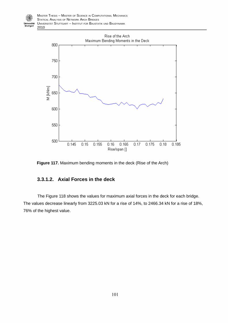
MASTER THESIS – MASTER OF SCIENCE IN COMPUTATIONAL MECHANICS
STATICAL ANALYSIS OF NETWORK ARCH BRIDGES
UNIVERSITÄT STUTTGART – INSTITUT FÜR BAUSTATIK UND BAUDYNAMIK
2010
Figure 117. Maximum bending moments in the deck (Rise of the Arch)
3.3.1.2. Axial Forces in the deck
The Figure 118 shows the values for maximum axial forces in the deck for each bridge.
The values decrease linearly from 3225.03 kN for a rise of 14%, to 2466.34 kN for a rise of 18%,
76% of the highest value.
PÁG.
101

MASTER THESIS – MASTER OF SCIENCE IN COMPUTATIONAL MECHANICS
STATICAL ANALYSIS OF NETWORK ARCH BRIDGES
UNIVERSITÄT STUTTGART – INSTITUT FÜR BAUSTATIK UND BAUDYNAMIK
2010
Figure 118. Maximum axial forces in the deck (Rise of the Arch)
3.3.1.3. Stresses in the deck
The Figure 119 shows the values for maximum stresses in the deck for each bridge. The
stresses decrease from a rise of 14% to a rise of 17.9%.
The maximum stress for a rise of 14% is 12023.53 kN/m2.. For a rise of 17.9% the stress is
10051.82 kN/m2, 84% of the highest value.
PÁG.
102

MASTER THESIS – MASTER OF SCIENCE IN COMPUTATIONAL MECHANICS
STATICAL ANALYSIS OF NETWORK ARCH BRIDGES
UNIVERSITÄT STUTTGART – INSTITUT FÜR BAUSTATIK UND BAUDYNAMIK
2010
Figure 119. Maximum stresses in the deck (Rise of the Arch)
3.3.1.4. Bending moments in the arch
The Figure 120 shows the absolute values for maximum bending moments in the arch for
each bridge. The curve fluctuates around a value of approximately 84 kNm. The fluctuations have
a magnitude of 20 kN, 23% of the previous value. The highest value occurs for a rise of 17.5%
and is equal to 104.44 kNm. The lowest value presents for a rise of 15.9% and it has value of
64.73 kNm.
PÁG.
103

MASTER THESIS – MASTER OF SCIENCE IN COMPUTATIONAL MECHANICS
STATICAL ANALYSIS OF NETWORK ARCH BRIDGES
UNIVERSITÄT STUTTGART – INSTITUT FÜR BAUSTATIK UND BAUDYNAMIK
2010
Figure 120. Maximum bending moments in the arch (Rise of the Arch)
3.3.1.5. Axial forces in the arch
The Figure 121 shows the values for maximum axial compression forces in the arch for
each bridge. The compression forces decrease linearly from -3757.05 kN for a rise of 14%, to
-3137.57 kN for a rise of 18%: 83% of the highest value.
PÁG.
104

MASTER THESIS – MASTER OF SCIENCE IN COMPUTATIONAL MECHANICS
STATICAL ANALYSIS OF NETWORK ARCH BRIDGES
UNIVERSITÄT STUTTGART – INSTITUT FÜR BAUSTATIK UND BAUDYNAMIK
2010
Figure 121. Maximum axial compression forces in the arch (Rise of the Arch)
3.3.1.6. Stresses in the arch
The Figure 122 shows the values for maximum stresses in the arch for each bridge. The
negative stresses decrease from -152557.50 kN/m2 at a rise of 14.2% to a value of -130315.31
kN/m2 at a rise of 17.9%: 85% of the highest value. The fluctuations in the curve have a
magnitude of 6000 kN/m2, 4% of the maximum negative stress.
PÁG.
105

MASTER THESIS – MASTER OF SCIENCE IN COMPUTATIONAL MECHANICS
STATICAL ANALYSIS OF NETWORK ARCH BRIDGES
UNIVERSITÄT STUTTGART – INSTITUT FÜR BAUSTATIK UND BAUDYNAMIK
2010
Figure 122. Maximum stresses in the arch (Rise of the Arch)
3.3.1.7. Stresses in the hangers
The Figure 123 shows the values for maximum stresses in the hangers for each bridge.
The stresses decrease from 144566.99 kN/m2 at a rise of 14.4% to a value of 135407.66 kN/m2 at
a rise of 18%: 94% of the highest value. The fluctuations in the curve have a magnitude of 1500
kN/m2, 1% of the highest value.
PÁG.
106

MASTER THESIS – MASTER OF SCIENCE IN COMPUTATIONAL MECHANICS
STATICAL ANALYSIS OF NETWORK ARCH BRIDGES
UNIVERSITÄT STUTTGART – INSTITUT FÜR BAUSTATIK UND BAUDYNAMIK
2010
Figure 123. Maximum stresses in the hangers (Rise of the Arch)
3.3.1.8. Relaxed hangers
There are no relaxed hangers in the bridges calculated.
3.3.2. Conclusions
The arch and the deck in the network arch bridges behave as the chords of a simply
supported beam: the arch being in compression and the deck being in tension. The axial forces in
the chords are inversely proporsional to the rise of the arch. As observed in the graphics for axial
forces in the deck and the arch, a higher ratio between the rise and the span reduce the
compression and tension forces in the chords.
This also occurs for the bending moments, but the reduction is much smaller.
Finally we can observe that the stresses in the arch, the deck and the hangers are reduce
as the ratio between the rise and the span is incremented.
Nevertheless the advantages of higher rises, aesthetic reason should be considered,
limiting the rise of the arch to values between 14% and 17%
PÁG.
107

MASTER THESIS – MASTER OF SCIENCE IN COMPUTATIONAL MECHANICS
STATICAL ANALYSIS OF NETWORK ARCH BRIDGES
UNIVERSITÄT STUTTGART – INSTITUT FÜR BAUSTATIK UND BAUDYNAMIK
2010
3.4. Number of hangers
In order to study the influence of the number of hangers 58 bridge are calculated. The
number of hangers in the models varies from 19 to 76.
A radial arrangement is used for this examination, with a cross angle of 45°. The bridge
configuration is shown in the Figure 65. This bridge has 38 hangers.
The results obtained for this bridge are:
− Maximum bending moment in the deck: 650.80 kNm
− Maximum axial force in the deck: 3045.90 kN
− Maximum Stress in the deck: 11507.07 kN/m2
− Maximum bending moment in the arch: -96.27 kNm
− Maximum axial force in the arch: -3642.89 kN
− Maximum stress in the arch: -146467.12 kN/m2
− Maximum stress in the hangers: 123037.74 kN/m2
− Number of relaxed hangers: 0
The number of element for the hangers is assigned as shown in the Figure C.2 in the
Appendix C.
3.4.1. Results
The results are showed in the following diagrams. Every ordinate corresponds to one value
of each bridge.
3.4.1.1. Bending moments in the deck
The Figure 124 shows the absolute values for maximum bending moments in the deck for
each bridge. The values become smaller as the number of hangers increase. However, the
decrease of the moments is higher for bridges with less than 30 hangers than for bridges with
more than 30 hangers. The bending moments decrease from 714.91 kNm for 19 hangers to
646.89 kNm for 31 hangers: a reduction of 10%. On the other hand, the maximum bending
moment for a bridge with 43 hangers is 635.89 kNm, a reduction of 2% in comparison with the
bending moment obtained for a bridge with 31 hangers.
PÁG.
108

MASTER THESIS – MASTER OF SCIENCE IN COMPUTATIONAL MECHANICS
STATICAL ANALYSIS OF NETWORK ARCH BRIDGES
UNIVERSITÄT STUTTGART – INSTITUT FÜR BAUSTATIK UND BAUDYNAMIK
2010
Figure 124. Maximum bending moments in the deck (Number of Hangers)
3.4.1.2. Axial forces in the deck
The Figure 125 shows the values for maximum axial forces in the deck for each bridge. As
the number of hangers is higher, the axial forces increase.
The maximum value for a bridge with 22 hangers is 2986.14 kN. For a bridge with 76 bridge the
axial force is equal to 3111.60 kN. This implies an increment of 4%.
PÁG.
109

MASTER THESIS – MASTER OF SCIENCE IN COMPUTATIONAL MECHANICS
STATICAL ANALYSIS OF NETWORK ARCH BRIDGES
UNIVERSITÄT STUTTGART – INSTITUT FÜR BAUSTATIK UND BAUDYNAMIK
2010
Figure 125. Maximum axial forces in the deck (Number of Hangers)
3.4.1.3. Stresses in the deck
The Figure 126 shows the values for maximum stresses in the deck for each bridge. The
values become smaller as the number of hangers increase. However, the decrease of the
stresses is higher for bridges with less than 30 hangers than for bridges with more than 30
hangers. The stresses decrease from 12259.63 kN/m2 for 19 hangers to 11431.33 kN/m2 for 31
hangers, a reduction of 7%. On the other hand, the maximum stress for a bridge with 43 hangers
is 11294.00 kN/m2, a reduction of 1% in comparison with the stress obtained for a bridge with 31
hangers.
PÁG.
110

MASTER THESIS – MASTER OF SCIENCE IN COMPUTATIONAL MECHANICS
STATICAL ANALYSIS OF NETWORK ARCH BRIDGES
UNIVERSITÄT STUTTGART – INSTITUT FÜR BAUSTATIK UND BAUDYNAMIK
2010
Figure 126. Maximum stresses in the deck (Number of Hangers)
3.4.1.4. Bending moments in the arch
The Figure 127 shows the absolute values for maximum bending moments in the arch for
each bridge. As the number of hangers becomes higher, the bending moments decrease.
The maximum value for a bridge with 19 hangers is 116.19 kN. For a bridge with 76 bridge the
bending moment is equal to -86.46 kN. The decrease of the absolute value of the bending
moments is of 26%.
PÁG.
111

MASTER THESIS – MASTER OF SCIENCE IN COMPUTATIONAL MECHANICS
STATICAL ANALYSIS OF NETWORK ARCH BRIDGES
UNIVERSITÄT STUTTGART – INSTITUT FÜR BAUSTATIK UND BAUDYNAMIK
2010
Figure 127. Maximum bending moments in the arch (Number of Hangers)
3.4.1.5. Axial forces in the arch
The Figure 128 shows the values for maximum axial compression forces in the arch for
each bridge. The compression forces become higher as the number of hangers increase.
The maximum compression force in a bridge with 19 hangers is -3574.47 kN, while for a
bridge with 76 hangers, it is -3789.41 kN. The increment is of 6%.
PÁG.
112

MASTER THESIS – MASTER OF SCIENCE IN COMPUTATIONAL MECHANICS
STATICAL ANALYSIS OF NETWORK ARCH BRIDGES
UNIVERSITÄT STUTTGART – INSTITUT FÜR BAUSTATIK UND BAUDYNAMIK
2010
Figure 128. Maximum axial compression forces in the arch (Number of Hangers)
3.4.1.6. Stresses in the arch
The Figure 129 shows the values for maximum stresses in the arch for each bridge. The
values decrease as the number of hangers increases. However, the decrease of the stresses is
higher for bridges with less than 35 hangers than for bridges with more than 35 hangers. The
values decrease from -157180.26 kN/m2 for 19 hangers to -146273.00 kN/m2 for 35 hangers, a
reduction of 7%. On the other hand, the maximum stress for a bridge with 51 hangers is
-144843.36 kN/m2, a reduction of 1% in comparison with the stress obtained for a bridge with 35
hangers.
There are fluctuations in the curve with a medium magnitude of 7000 kN/m2, 4% of the highest
value.
PÁG.
113

MASTER THESIS – MASTER OF SCIENCE IN COMPUTATIONAL MECHANICS
STATICAL ANALYSIS OF NETWORK ARCH BRIDGES
UNIVERSITÄT STUTTGART – INSTITUT FÜR BAUSTATIK UND BAUDYNAMIK
2010
Figure 129. Maximum stresses in the arch (Number of Hangers)
3.4.1.7. Stresses in the hangers
The Figure 130 shows the values for maximum stresses in the hangers for each bridge.
The stresses decrease as the number of hangers increases. However, the decrease of the
stresses is higher for bridges with less than 50 hangers than for bridges with more than 50
hangers. The values decrease from 216613.45 kN/m2 for 24 hangers to 114323.32 kN/m2 for 50
hangers, a reduction of 47%. On the other hand, the maximum stress for a bridge with 76 hangers
is 80685.07 kN/m2, a reduction of 29% in comparison with the stress obtained for a bridge with 50
hangers.
PÁG.
114

MASTER THESIS – MASTER OF SCIENCE IN COMPUTATIONAL MECHANICS
STATICAL ANALYSIS OF NETWORK ARCH BRIDGES
UNIVERSITÄT STUTTGART – INSTITUT FÜR BAUSTATIK UND BAUDYNAMIK
2010
Figure 130. Maximum stresses in the hangers (Number of Hangers)
3.4.1.8. Relaxed hangers
The Figure 131 shows the number of relaxed hangers for each bridge. As the number of
hangers increase, the tendency of the hangers to relax also increase. For bridges with a number
of hangers between 20 and 38 there are no relaxed hangers. From 39 to 45, the number of
relaxed hangers varies between 1 and 0. Again, between 46 and 55 no relaxation of the hangers
is found.
For a number of hangers between 56 and 74 the number of relaxed hangers varies
between 1 and 2. A bridge with 75 hangers presents 3 relaxed hangers.
The relaxed elements are located in the extremes of the bridge, next to the supports.
PÁG.
115

MASTER THESIS – MASTER OF SCIENCE IN COMPUTATIONAL MECHANICS
STATICAL ANALYSIS OF NETWORK ARCH BRIDGES
UNIVERSITÄT STUTTGART – INSTITUT FÜR BAUSTATIK UND BAUDYNAMIK
2010
Figure 131. Relaxed hangers (Number of Hangers)
3.4.2. Conclusions
High number of hangers results in lower values for the stresses in arch, deck and hangers.
However, the influence of the number of hangers over the bending moments in the deck is
higher for a small number of hangers: a small variation in the number of hangers will cause a
higher variation of the bending moments if the bridge has less than 30 hangers.
As the influence of the number of hangers over the axial forces in the deck and the arch is
very small (less than 6%), the variation of the stresses follows the variation of the bending
moments. For this reason, the influence of the number of hangers over the stresses is higher
when the bridge has a small number of hangers: less than 30 in the case of the deck; less than 35
in the case of the arch.
The same applies for the stresses in the hangers: the influence is higher for bridges with
small number of hangers: less than 50.
Always considering aesthetic matters, no more that 40 hangers should be used. After this
point the decrease in the stresses as the number of hangers increase is not important, and for
more than 40 hanger, relaxation occur.
PÁG.
116

MASTER THESIS – MASTER OF SCIENCE IN COMPUTATIONAL MECHANICS
STATICAL ANALYSIS OF NETWORK ARCH BRIDGES
UNIVERSITÄT STUTTGART – INSTITUT FÜR BAUSTATIK UND BAUDYNAMIK
2010
Chapter 4
Study of Alternatives
For this Chapter, three different alternatives to the original configuration are proposed.
Considering the studies from Chapter 3, two parameters are chosen for the comparison:
the hanger arrangement and the shape of the arch. In the alternative configurations no changes
are made regarding the rise of the arch or the number of hangers. It is considered that this
parameters are not important in comparison with the chosen ones. Besides, maintaining the rise
of the arch and the number of hangers in the different alternatives provides a better point of
comparison between the three systems.
The Section 4.1 presents the three alternatives with a brief description of each one.
In the Section 4.2 the results obtained are analyzed and compared.
Finally, the conclusions and final overlook are exposed in the Section 4.3.
4.1. Proposed Configurations
4.1.1. Original Configuration
The proposed alternatives are compared with the original configuration of the Lužnice
Bridge, described in the Chapter 2. In this case the prestressing of the hangers is considered in
order to avoid relaxation.
4.1.2. Alternative A
In network arch bridges, a correct choice of the hangers arrangement can improve
significantly the stresses in deck, arch and hangers. For the Alternative A, some characteristics of
the original bridge are maintained (number of hangers, rise of the arch) and a different
configuration of the hangers is proposed.
The alternative A is based in the configuration presented in the Section 3.1.1. : an
arrangement based on the linear variation of the slopes. A circular arch shape is used and
prestressing of the hangers is not considered.
For this configurations, the lowest stresses in the deck and the arch present for small initial
angles and large angle increments. However, this arrangements results in the highest stresses in
PÁG.
117

MASTER THESIS – MASTER OF SCIENCE IN COMPUTATIONAL MECHANICS
STATICAL ANALYSIS OF NETWORK ARCH BRIDGES
UNIVERSITÄT STUTTGART – INSTITUT FÜR BAUSTATIK UND BAUDYNAMIK
2010
the hangers. On the other hand, to obtained small stresses in the hangers large initial angles and
small angle increments should be chosen, resulting in high stresses for arch and deck. In addition,
small initial angles and small angles increments cause relaxation of the hangers. Hence, hanger
arrangements with large initial angles and large angle increments should be used.
An initial angle of 81° and an increment angle of 3 .4° are chosen. The Figure 132 shows a
bridge that corresponds to this configuration.
Figure 132. Alternative A
4.1.3. Alternative B
For the Alternative B, the number of hangers and rise of the arch of the original bridge are
maintained and a different configuration of the hangers is proposed.
The alternative B is based in the configuration presented in the Section 3.1.2.: the radial
arrangement, proposed by Brunn and Schanack in their diploma thesis [BSC].
In the radial arrangement the lowest stresses for the arch and the deck are obtained for
cross angles between 40° and 50°. The lowest stress es in the hangers present for cross angles
smaller than 30°. However, the rate of increment fo r angles smaller than 50° is not important.
A cross angle of 41.5° is chosen. The Figure 133 sh ows a bridge that corresponds to this
configuration.
Figure 133. Alternative B
PÁG.
118

MASTER THESIS – MASTER OF SCIENCE IN COMPUTATIONAL MECHANICS
STATICAL ANALYSIS OF NETWORK ARCH BRIDGES
UNIVERSITÄT STUTTGART – INSTITUT FÜR BAUSTATIK UND BAUDYNAMIK
2010
4.1.4. Alternative C
For the alternative C, all the characteristics of the original configuration are maintained, with
the exception of the shape of the arch. While the form of the arch in the Lužnice Bridge is fully
parabolic, for this alternative a circular arch shape arch is proposed with a parabolic shape in the
extremes.
This configuration is chosen in order to examine the possibility of avoiding the prestressing
of the hangers, and to study the shape of the arch as an alternative to prevent relaxation. Hence,
the variables are defined in order to obtain no relaxed hangers.
The variables adopted are: a radio RREL 1.2 times the one obtained for a fully circular arch;
and the distance long1, from where the circular arch begins, equal to 6.15 m: 15% of the span of
the bridge. The Figure 89 shows this variables.
The Figure 134 shows a bridge that corresponds to this configuration.
Figure 134. Alternative C
PÁG.
119

MASTER THESIS – MASTER OF SCIENCE IN COMPUTATIONAL MECHANICS
STATICAL ANALYSIS OF NETWORK ARCH BRIDGES
UNIVERSITÄT STUTTGART – INSTITUT FÜR BAUSTATIK UND BAUDYNAMIK
2010
4.2. Comparison of Alternatives
4.2.1. Stresses in the deck
The Figure 135 shows the maximum and minimum stresses in the deck, for each
coordinate.The curves correspond to the original configuration, and the three alternatives.
For the original configuration, the highest values for the maximum stresses in the deck
occur in two peaks, at 25% and 75% of the span: 13590.88 kN/m2 and 16395.36 kN/m2
respectively.
The Alternatives A and B also present the highest values for the maximum stresses in two
peaks. The position of the first peak coincides approximatly with the position for the original
configuration, at 25% of the span. For the Alternative A, it has a value of 9317.21 kN/m2 : 69% of
the original stress. For the Alternative B, it has a value of 8263.14 kN/m2 : 60% of the original
stress.
For the Alternatives A and B the second peak has the form of a “plateau” from 22 m to 33
m from the left support (50% to 80% of the span). For the Alternative A, it has a value of 11983.45
kN/m2 : 73% of the original stress. For the Alternative B, it has a value of 11496.77 kN/m2 : 70% of
the original stress.
On the other hand, the Alternative C presents three peaks, at 15%, 60% and 85% of the
span. The stresses for the two higher peaks are 24107.60 kN/m2 and 21023.61 kN/m2 , wich are
1.47 and 1.28 times the highest value for the original configuration.
The smaller peak has a stress of 12467.09 kN/m2, 90% of the original stress for this
coordinate: 13867.63 kN/m2. From this point to the end of the span, the stresses for the
Alternative C are smaller than the stresses for the original configuration, always with a reduction of
between 70% and 90%.
PÁG.
120

MASTER THESIS – MASTER OF SCIENCE IN COMPUTATIONAL MECHANICS
STATICAL ANALYSIS OF NETWORK ARCH BRIDGES
UNIVERSITÄT STUTTGART – INSTITUT FÜR BAUSTATIK UND BAUDYNAMIK
2010
Figure 135. Comparison of Alternatives. Stresses in the deck
4.2.2. Stresses in the arch
The Figure 136 shows the maximum and minimum stresses in the arch, for each
coordinate.The curves correspond to the original configuration, and the three alternatives.
The minimum value for the stresses in the original configuration is -175209.09 kN/m2 and it
is located 25 m from the left support, 60% of the span.
The curves that correspond to the Alternatives A and B have similar form and values. The
stresses for the Alternative B are slightly smaller.
The minimum stress for the Alternative A is -145173.62 kN/m2, 83% of the original stress.
For the Alternative B the minimum stress is -141853.09 kN/m2, 81% of the original value.
The minimum stress for the Alternative C is -224866.74 kN/m2, 1.28 times the original
stress.
In all the cases, the highest values for the maximum stresses occur in three peaks, at
10%, 50% and 85%. For the original configuration the highest value occurs in the second peak,
while for the alternatives it happens in the first peak.
PÁG.
121

MASTER THESIS – MASTER OF SCIENCE IN COMPUTATIONAL MECHANICS
STATICAL ANALYSIS OF NETWORK ARCH BRIDGES
UNIVERSITÄT STUTTGART – INSTITUT FÜR BAUSTATIK UND BAUDYNAMIK
2010
Figure 136. Comparison of Alternatives. Stresses in the arch
4.2.3. Stresses in the hangers
The Figure 137 shows the maximum stresses for each hanger for the Set 1. The curves
correspond to the original configuration, and the three alternatives. The number of elements for
the hangers were assigned as is shown in the Figure C.1 of the Appendix C.
All cases present no relaxed hangers. To achieved this it is necessary to prestress the
hangers 3019 and 3018 in the original configuration. No prestressing was done for any of the
Alternatives.
The maximum stress for the original configuration corresponds to the hanger 3019 and it is
equal to 210373.47 kN/m2.
The curves than correspond to the Alternatives A and B are very similar for the hangers
3001 to 3015. There is an increment of the stresses in the Alternative B for the hangers 3016 and
3017. The increment is of less than 35%.
The stresses for the Alternatives A and B are lower than the original stresses for most of the
hangers. The exceptions are the hangers 3003 and 3005. As the hanger is closer to the right
support, the difference between the curve of the original configuration and the curve of the
PÁG.
122

MASTER THESIS – MASTER OF SCIENCE IN COMPUTATIONAL MECHANICS
STATICAL ANALYSIS OF NETWORK ARCH BRIDGES
UNIVERSITÄT STUTTGART – INSTITUT FÜR BAUSTATIK UND BAUDYNAMIK
2010
alternatives becomes more important, with a significant reduction of the stresses in the
Alternatives A and B.
The maximum stress for the Alternative A corresponds to the hanger 3018 and it is equal to
105313.00 kN/m2, 50% of the stress that corresponds to the original configuration.
The maximum stress for the Alternative B corresponds to the hanger 3017 and it is equal to
118269.21 kN/m2, 56% of the stress that corresponds to the original configuration.
The stresses for the Alternative C are inferior than the stresses for the original configuration
for the hangers 3005 to 3019, following approximately the same form of the curve . This case
present the smallest stress for the hanger 3019, 20% of the original value. However, the stresses
for the hangers 3001, 3002 and 3003 are more than four times higher than the original stresses.
These hangers are located in the zone where the arch becomes parabolic.
The maximum stress for the Alternative C corresponds to the hanger 3003 and it is equal to
236904.39 kN/m2, 1.13 times the stress that corresponds to the original configuration.
The Figures 138 shows the maximum stresses for each hanger for the Set 2. The curves
correspond to the original configuration, and the three alternatives.
Again, all cases present no relaxed hangers. To achieved this it is necessary to prestress
the hangers 3037 and 3038 in the original configuration. No prestressing was done for any of the
Alternatives.
The maximum stress for the original configuration corresponds to the hanger 3038 and it is
equal to 126360.12 kN/m2.
The curves than correspond to the Alternative A and B have similar form and values. The
stresses are higher than the original stresses for most of the hangers. The exception is the hanger
3038. The difference is of the order of 65000 kN/m2.
The maximum stress for the Alternative A corresponds to the hanger 3035 and it is equal to
128092.29 kN/m2, 1.01 times the higher value that corresponds to the original configuration.
The maximum stress for the Alternative B corresponds to the hanger 3017 and it is equal to
135372.90 kN/m2, 1.07 times the higher value that corresponds to the original configuration.
The stresses for the Alternative C are inferior than the stresses for the original configuration
for the hangers 3024 to 3038, following approximately the same form of the curve. However, the
stresses for the hangers 3020 to 3024 are more than seven times higher than the original
stresses. These hangers are located in the zone where the arch becomes parabolic.
The maximum stress for the Alternative C corresponds to the hanger 3021 and it is equal to
238099.14 kN/m2, 1.88 times the stress that corresponds to the original configuration.
PÁG.
123

MASTER THESIS – MASTER OF SCIENCE IN COMPUTATIONAL MECHANICS
STATICAL ANALYSIS OF NETWORK ARCH BRIDGES
UNIVERSITÄT STUTTGART – INSTITUT FÜR BAUSTATIK UND BAUDYNAMIK
2010
Figure 137. Comparison of Alternatives. Stresses in the hangers for the Set 1
Figure 138. Comparison of Alternatives. Stresses in the hangers for the Set 2
PÁG.
124
MASTER THESIS – MASTER OF SCIENCE IN COMPUTATIONAL MECHANICS
STATICAL ANALYSIS OF NETWORK ARCH BRIDGES
UNIVERSITÄT STUTTGART – INSTITUT FÜR BAUSTATIK UND BAUDYNAMIK
2010
4.3. Conclusions
From the analysis of the results obtained for the Alternatives A and B in the Figure 135 to 138
of the previous section, it can be noticed how a good choice of the hanger arrangement could
improve the stresses in the elements of a bridge.
The results for this two alternatives are surprisingly similar. In the case of the arch and the
deck, the form of the curves is similar to the one obtained for the original configuration, with lower
values: 70% for the deck and 80% for the arch.
For the stresses in the hangers, however, lower values are only obtained for the Set 1. In this
case the form of the curve approximate in a certain way to the one obtained for the original
configuration, with an important improvement of the stresses: a reduction of 50%. The decrease of
the stresses is specially noticeable for the hanger 3019. In the original configuration this hanger was
prestressed, in order to avoid its relaxation. Because of the prestressing force, the stress for this
hanger is significantly higher than the others. In the Alternatives A and B the relaxation of the hanger
3019 was avoided without prestressing, hence the maximum stress for this element is drastically
reduce.
The Figure 138 shows the maximum stresses in the hangers for the Set 2. In this Figure it can
be observed that the form of the curve for the Alternatives A and B differs from the form that
correspond to the original configuration, presenting higher values for most of the hangers. However,
the highest stress for the Alternatives A and B is of the same order than the highest stress for the
original configuration.
The curve for the original configuration shows small stresses for all hangers, except the hanger
3038, that presents a value 2.50 times higher. This occurs because this hanger is prestressed. The
stress in the hanger 3019 is 50% smaller for the Alternatives A and B, as these cases present no
prestressing.
According to [NAB] all hangers must have the same cross-section. Hence, is desirable to have
the smallest possible variation of the maximum stresses in the hangers. This variation is 201630 kN/
m2 for the original configuration, 110620 kN/m2 for the Alternative A and 115700 kN/m2 for the
Alternative B. This implies a reduction of 50% in the Alternatives A and B.
Besides, as all hangers must have the same cross section, this parameter should be chosen
according to the highest maximum stress. Comparing the highest maximum stress for the
Alternatives A and B with the maximum stress for the original configuration for all hangers, the values
for the alternatives are 60% smaller.
Hence, the improvement obtained with the Alternatives A and B is evident.
PÁG.
125

MASTER THESIS – MASTER OF SCIENCE IN COMPUTATIONAL MECHANICS
STATICAL ANALYSIS OF NETWORK ARCH BRIDGES
UNIVERSITÄT STUTTGART – INSTITUT FÜR BAUSTATIK UND BAUDYNAMIK
2010
The Alternatives A and B presents similar results. Besides, in the Figures 132 and 133 it can be
noticed that the configurations are similar. It is curious how using two different methods (Sections
3.1.1 and 3.1.2) similar solutions have been reached.
Regarding the Alternative C, the objective is to propose a different solution for the problem of
the relaxation of the hangers. The effect of a change in the form at the ends of the arch is studied.
While the original configuration presented four relaxed hangers near the supports, the configuration
proposed in the Section 4.1.4. presents none.
However, even if this goal is achieved, the stresses obtained for the Alternative C are
significantly higher than in the rest of the cases. The maximum value obtained for this alternative is
1.30 times the maximum value obtained for the original configuration, in both deck and arch.
Regarding the hangers, the stresses for the Alternative C are lower than for the original
configuration, except for the hangers near the left support. For this elements the stress increase
drastically, arriving to values seven times higher than the original. On the other hand, the stresses for
the hangers near the right support are significantly reduced.
Therefore, while the Alternative C gives good results for the hangers in the center and near the
right support, decreasing the stresses and avoiding relaxation, it presents an important increment of
the stresses in the deck, the arch, and the hangers near the left support. This makes of the
Alternative C an unsuitable solution.
Finally, it can be concluded that the Alternatives A and B presents the lowest stresses and the
most effective force distribution.
However, more practical issues should be considered. While the total length of the hangers for
the original configuration is 182.76 m, it is 217.61 m for the Alternative A and 230.06 for the
Alternative B. This means that the length of the hangers is 20% larger for the first alternative and 26%
for the second alternative. This implies a higher economical cost, and a larger area exposed to the
wind.
Moreover, while in the original configuration the hangers cross each other two times, in the
Alternatives A and B the hangers cross each other 6 times. This should be considered as too many
intersections of the hangers can complicate replacements in case of breaking.
As it can be seen, even if for Alternatives A and B lower stresses are obtain, a particular study
should be done for each bridge, considering constructive and economical aspects, in order to find the
most adequate solution.
PÁG.
126

MASTER THESIS – MASTER OF SCIENCE IN COMPUTATIONAL MECHANICS
STATICAL ANALYSIS OF NETWORK ARCH BRIDGES
UNIVERSITÄT STUTTGART – INSTITUT FÜR BAUSTATIK UND BAUDYNAMIK
2010
Chapter 5
Summary
The intention of this work is to study the different parameters that influence the structural
behavior of network arch bridges. As a particular example, the bridge over the river Lužnice in the
Czech Republic is chosen.
After an analysis of the Lužnice bridge in the Chapter 2, the worst loading assumptions for
the bridge are determined: the load case LC1 (Load Model 1 [E1-2]), with the live load applied
only in the right half of the span.
Considering this, four different parameters are studied in the Chapter 3: hanger
arrangement, form of the arch, rise of the arch and number of hangers.
As the hanger arrengement constitutes the main characteristic of the network arch bridge,
special emphasis is placed in this parameter. Two arrangements are studied.
The Section 3.1.1. analyze hanger arrengements based on the linear variation of the
slopes. It is found that it is not recommendable to use configurations with small initial angles and
large angle increments or large initial angles and small angle increments. This is because while
the first case presents small stresses in the deck and the arch but high stresses in the hangers,
the second case presents small stresses in the hangers, but high stresses in the deck and the
arch. In addition, configurations with small initial angles and small angle increments present
relaxed hangers. Hence, the best solutions are obtained with large initial angles and large angle
increments.
The Section 3.1.2. examine radial arrangements, as proposed for Brunn and Schanack in
their diploma thesis [BSC]. It is found that the best results are obtained for cross angles between
40° and 50°.
In the Section 3.2. the variation of the shape of the arch is analyzed. It is found that a
slightly change in the form of the arch could be a solution for the problem of the relaxation of the
hangers. However, it also causes the stresses in the elements to increase drastically.
The Section 3.3. examine the effects of the rise of the arch. As expected, an increment in
the ratio between the rise and the span reduce the stresses in the arch, the deck and the hangers.
Nevertheless, due to aestethic reasons the rise of the arch should be between 14% and 17%.
In the Section 3.4. the influence of the number of hangers is analyzed. An increment in the
number of hangers implies a decrease of the stresses in arch, deck and hangers. It is not
recommendable to use more than 40 hangers, as at this point relaxation occur.
PÁG.
127
MASTER THESIS – MASTER OF SCIENCE IN COMPUTATIONAL MECHANICS
STATICAL ANALYSIS OF NETWORK ARCH BRIDGES
UNIVERSITÄT STUTTGART – INSTITUT FÜR BAUSTATIK UND BAUDYNAMIK
2010
Considering the conclusions of Chapter 3, three alternatives are proposed in Chapter 4:
The Alternative A presents an arrangement based on the linear variation of the slopes with an
initial angle of 81° and increment angle of 3.4°; t he Alternative B presents a radial arrangement
with a cross angle of 41.5°; and the Alternative C proposes a circular arch with a parabolic shape
in the extremes, maintaining the original hanger arrangement. Prestressing is only considered in
the original configuration.
Comparing the stresses obtained for the alternatives with the original configuration, the
best results are obtained for the Alternatives A and B. The Alternative C presents high values for
the stresses in the deck, the arch, and the hangers near the left support. None of the alternatives
present relaxed hangers. Alternatives A and B presents similar results.
However, more practical issues should be considered, as total length of the hangers and
number of intersection between them, in order to find the most adequate solution.
PÁG.
128

MASTER THESIS – MASTER OF SCIENCE IN COMPUTATIONAL MECHANICS
STATICAL ANALYSIS OF NETWORK ARCH BRIDGES
UNIVERSITÄT STUTTGART – INSTITUT FÜR BAUSTATIK UND BAUDYNAMIK
2010
Appendix A
Sections of the Lužnice Bridge
Figure A.1 Cross section of the Lužnice Bridge [DSL]
PÁG.
129

MASTER THESIS – MASTER OF SCIENCE IN COMPUTATIONAL MECHANICS
STATICAL ANALYSIS OF NETWORK ARCH BRIDGES
UNIVERSITÄT STUTTGART – INSTITUT FÜR BAUSTATIK UND BAUDYNAMIK
2010
Figure A.2. Longitudinal section of the Lužnice Bridge [DSL]
PÁG.
130

MASTER THESIS – MASTER OF SCIENCE IN COMPUTATIONAL MECHANICS
STATICAL ANALYSIS OF NETWORK ARCH BRIDGES
UNIVERSITÄT STUTTGART – INSTITUT FÜR BAUSTATIK UND BAUDYNAMIK
2010
Appendix B
Results for the Lužnice Bridge
Table B.1. Maximum and minimum bending moments and axial forces for the deckelements (Even Load)
PÁG.
131

MASTER THESIS – MASTER OF SCIENCE IN COMPUTATIONAL MECHANICS
STATICAL ANALYSIS OF NETWORK ARCH BRIDGES
UNIVERSITÄT STUTTGART – INSTITUT FÜR BAUSTATIK UND BAUDYNAMIK
2010
Table B.2. Maximum and minimum stresses for the deck elements (Even Load)
PÁG.
132

MASTER THESIS – MASTER OF SCIENCE IN COMPUTATIONAL MECHANICS
STATICAL ANALYSIS OF NETWORK ARCH BRIDGES
UNIVERSITÄT STUTTGART – INSTITUT FÜR BAUSTATIK UND BAUDYNAMIK
2010
Table B.3. Maximum and minimum bending moments and axial forces for the deckelements (Partial Load)
PÁG.
133

MASTER THESIS – MASTER OF SCIENCE IN COMPUTATIONAL MECHANICS
STATICAL ANALYSIS OF NETWORK ARCH BRIDGES
UNIVERSITÄT STUTTGART – INSTITUT FÜR BAUSTATIK UND BAUDYNAMIK
2010
Table B.4. Maximum and minimum stresses for the deck elements (Partial Load)
PÁG.
134

MASTER THESIS – MASTER OF SCIENCE IN COMPUTATIONAL MECHANICS
STATICAL ANALYSIS OF NETWORK ARCH BRIDGES
UNIVERSITÄT STUTTGART – INSTITUT FÜR BAUSTATIK UND BAUDYNAMIK
2010
Table B.5. Maximum and minimum bending moments and axial forces for the archelements (Even Load).
PÁG.
135

MASTER THESIS – MASTER OF SCIENCE IN COMPUTATIONAL MECHANICS
STATICAL ANALYSIS OF NETWORK ARCH BRIDGES
UNIVERSITÄT STUTTGART – INSTITUT FÜR BAUSTATIK UND BAUDYNAMIK
2010
Table B.6. Maximum and minimum stresses for the arch elements (Even Load)
PÁG.
136

MASTER THESIS – MASTER OF SCIENCE IN COMPUTATIONAL MECHANICS
STATICAL ANALYSIS OF NETWORK ARCH BRIDGES
UNIVERSITÄT STUTTGART – INSTITUT FÜR BAUSTATIK UND BAUDYNAMIK
2010
Table B.7. Maximum and minimum bending moments and axial forces for the archelements (Partial Load)
PÁG.
137

MASTER THESIS – MASTER OF SCIENCE IN COMPUTATIONAL MECHANICS
STATICAL ANALYSIS OF NETWORK ARCH BRIDGES
UNIVERSITÄT STUTTGART – INSTITUT FÜR BAUSTATIK UND BAUDYNAMIK
2010
Table B.8. Maximum and minimum stresses for the arch elements (Partial Load)
PÁG.
138

MASTER THESIS – MASTER OF SCIENCE IN COMPUTATIONAL MECHANICS
STATICAL ANALYSIS OF NETWORK ARCH BRIDGES
UNIVERSITÄT STUTTGART – INSTITUT FÜR BAUSTATIK UND BAUDYNAMIK
2010
Table B.9. Maximum and minimum stresses for the hanger elements (Even Load)
PÁG.
139

MASTER THESIS – MASTER OF SCIENCE IN COMPUTATIONAL MECHANICS
STATICAL ANALYSIS OF NETWORK ARCH BRIDGES
UNIVERSITÄT STUTTGART – INSTITUT FÜR BAUSTATIK UND BAUDYNAMIK
2010
Table B.10. Maximum and minimum stresses for the hanger elements (Partial Load)
PÁG.
140

MASTER THESIS – MASTER OF SCIENCE IN COMPUTATIONAL MECHANICS
STATICAL ANALYSIS OF NETWORK ARCH BRIDGES
UNIVERSITÄT STUTTGART – INSTITUT FÜR BAUSTATIK UND BAUDYNAMIK
2010
Appendix C
Numbers assigned to hanger elements
Set 1
Set 2
Figure C.1. Numbers assigned to hanger elements (Original hanger arrangement andhanger arrangements based on the linear variation of the slopes)
Set 1
Set 2
Figure C.2. Numbers assigned to hanger elements (Radial arrangements)
PÁG. Z
141

MASTER THESIS – MASTER OF SCIENCE IN COMPUTATIONAL MECHANICS
STATICAL ANALYSIS OF NETWORK ARCH BRIDGES
UNIVERSITÄT STUTTGART – INSTITUT FÜR BAUSTATIK UND BAUDYNAMIK
2010
PÁG. Z
142

MASTER THESIS – MASTER OF SCIENCE IN COMPUTATIONAL MECHANICS
STATICAL ANALYSIS OF NETWORK ARCH BRIDGES
UNIVERSITÄT STUTTGART – INSTITUT FÜR BAUSTATIK UND BAUDYNAMIK
2010
Appendix D
Input File
The input file for the radial arrangement of Section 3.1.2. can be found here. This ispresented as an example of the codes used in this thesis. The definitions of the commands areobtained from [Ahlp].
D.1. Preliminary Definitions
Commands for clearing the database and entering the model creation preprocesor.FI�ISH
/CLEAR
/PREP7
D.2. Definition of Parameters
D.2.1. Geometry and dimensions
- Span of the bridgespan=41
- Rise of the bridge, expressed as percentage of the spanw=6.05/span
- Number of hangersnh = 38
- lsmall limits the minimum length of an element in the deck and the arch, as explain inSection D.3.3.
lsmall=0.2
- Geometry of the circular archr=span*w
c=span/2
d=r/2-span**2/(8*r)
Ra=sqrt(c**2+d**2)
D.2.1.1. Deck
- Parameters for the effective cross sectiondb=1.090
dh=0.56
db1=1.085*0.2+0.1*(1.5*1.085)
dh1=0.18
db2=1.8*0.2+0.1*(0.7*1.8*2)
PÁG.
143

MASTER THESIS – MASTER OF SCIENCE IN COMPUTATIONAL MECHANICS
STATICAL ANALYSIS OF NETWORK ARCH BRIDGES
UNIVERSITÄT STUTTGART – INSTITUT FÜR BAUSTATIK UND BAUDYNAMIK
2010
dh2=0.275
- Parameters for the real cross sectiondbreal=1.090
dhreal=0.56
db1real=1.085
dh1real=0.18
db2real=1.8
dh2real=0.275
- Areas and moment of inertiaAread=db*dh+db1*dh1+db2*dh2
Id=1/12*db*dh**3
Id=Id+db1*dh1*(dh/2-dh1/2)**2
Id=Id+db2*dh2*(dh/2-dh2/2)**2
Areadreal=dbreal*dhreal+db1real*dh1real+db2real*dh2real
D.2.1.2. Arch
- Parameters for the cross sectionah=0.32
at=0.035
- Area and moment of inertiaAreaa=ah*at+2*at*(ah-at)
Ia=2*1/12*at*ah**3+(ah-2*at)*at*(ah/2-at/2)**2
D.2.1.3. Hangers
- Parameters for the cross sectionhd=0.04
- Area and moment of inertiaAreah=3.14159*hd**2/4
Ih=3.14159*hd**4/64
D.2.2. Material and Loading properties
- Elastic modulusEsteel=2e8
Econcr=2.99e7
- Self weightGsteel=7.8
Gconcr=2.5
PÁG.
144

MASTER THESIS – MASTER OF SCIENCE IN COMPUTATIONAL MECHANICS
STATICAL ANALYSIS OF NETWORK ARCH BRIDGES
UNIVERSITÄT STUTTGART – INSTITUT FÜR BAUSTATIK UND BAUDYNAMIK
2010
- Limit coordinates of the portion of the span where the live load is applied.LongLL1=0.5
longLL2=1
l1=span*longLL1
l2=span*longLL2
- Distance between two consecutives positions of the moving load.lstep=1
- Partial factors:gammaSteel=1.20
gammaConcr=1.35
- Parameters for load combination LM1qLM1=15.38
pLM1=87.35
- Dead loadqDL=5.06+Areadreal*Gconcr*9.8
D.2.3. Cross angles for the Radial Arrangement
Radang1 = 0
Radang2 = 57
Radangstep = 0.5
D.2.4. Definition of Matrices
These matrices are used to store the results obtained for each bridge.
- Deck*DIM,Matrixd,ARRAY,(Radang2-Radang1)/Radangstep+1,10
*vfill,Matrixd(1,1),ramp,radang1,radangstep
- Arch*DIM,Matrixa,ARRAY,(Radang2-Radang1)/Radangstep+1,10
*vfill,Matrixa(1,1),ramp,radang1,radangstep
- Hangers*DIM,Matrixh,ARRAY,(Radang2-Radang1)/Radangstep+1,10
*vfill,Matrixh(1,1),ramp,radang1,radangstep
PÁG.
145

MASTER THESIS – MASTER OF SCIENCE IN COMPUTATIONAL MECHANICS
STATICAL ANALYSIS OF NETWORK ARCH BRIDGES
UNIVERSITÄT STUTTGART – INSTITUT FÜR BAUSTATIK UND BAUDYNAMIK
2010
D.3. Geometry of the bridge
D.3.1. Loop
*do,Radang,Radang1, Radang2,Radangstep
In the beginning of each loop, the model creation preprocesor is accessed and all theelements of the previous bridges are erased.
/prep7
lsdele,all
lclear,all
ldele,all
kdele,all
D.3.2. Geometry of arch and deck
Several lines are defined following the geometry of the arch. Using the command LCOMBthe lines are combined into one. This line is divided in equal parts according to the number ofhangers nh.
In the same way, the deck is divided according to the number of hangers nh.
k,1000,0,0
numstr,line,1000
*do,i,1,m
x = span/m*i
y = sqrt(Ra**2-(x-c)**2)+d
k,1000+i,x,y
l,999+i,1000+i
*enddo
kmodif,1000+m,,0
LCOMB,all
l,1000,1000+m
- Division of the archnumstr,line,501
numstr,kp,501
Larch=2*Ra*ACOS((Ra-r)/Ra)
narch=(nh+1)*nint(Larch/(nh+1))
LDIV,1000,,,narch,1
PÁG.
146

MASTER THESIS – MASTER OF SCIENCE IN COMPUTATIONAL MECHANICS
STATICAL ANALYSIS OF NETWORK ARCH BRIDGES
UNIVERSITÄT STUTTGART – INSTITUT FÜR BAUSTATIK UND BAUDYNAMIK
2010
- Division of the deck
numstr,line,702
numstr,kp,701
ndeck=(nh+1)*nint(span/(nh+1))
LDIV,1001,,,ndeck,0
ldele,1001
numstr,line,701
l,1000,701
D.3.3. Hanger arrangement
The number of hangers for the Set1 nh1 and for the Set 2 nh2 are obtained.
nh2=nint(nh/2)
*if,nh2,eq,nh/2,then
nh1=nh2
*else
nh1=nh2-1
*endif
The hanger arrangement is created with a loop. In each step, the coordinate xo from wherethe hanger starts is obtained and the angle of the radial direction of the arch in this point iscalculated as alfa. The cross angle Radang is consecutively added and subtracted from alfa, andthe final point x1 of the hanger is found. Finally, the line element is created.
numstr,line,801
numstr,kp,800
RadangAux=Radang/180*3.14
*do,l,1,nh
xo=kx(500+(l*nint(Larch/(nh+1))))
alfa=3.14/2-ATA�(-(xo-c)/sqrt(Ra**2-(xo-c)**2))
rot=(-1)**l
y1=ky(500+(l*nint(Larch/(nh+1))))
x1=xo+y1/tan(alfa+RadangAux*rot)
k,800+l,x1,0
l,800+l,500+(l*nint(Larch/(nh+1)))
*enddo
numstr,line,701
lsel,s,line,,801,800+nh,2,0
lsel,a,line,,701,799,1,0
lglue,all
lsel,s,line,,802,800+nh,2,0
lsel,a,line,,701,799,1,0
lglue,all
PÁG.
147

MASTER THESIS – MASTER OF SCIENCE IN COMPUTATIONAL MECHANICS
STATICAL ANALYSIS OF NETWORK ARCH BRIDGES
UNIVERSITÄT STUTTGART – INSTITUT FÜR BAUSTATIK UND BAUDYNAMIK
2010
lsel,all
ldele,1000
D.3.4. Enhancement of the model
After running the precedent codes, the model obtained could present some inconvenients:lines too large, different directions of the normals between adjacent elements, or disorderednumbering. The following codes correct these problems.
D.3.4.1. Deck
The first and last keypoints of the deck are renamed, as well as the numbering of the linesthat belong to the deck. The maximum number assign to the lines is obtained as lmaxd.
numstr,kp,1
k,1,0,0
k,2,span,0
numstr,line,2501
lgen,2,701,799,1,0,0,0,0,0,0
ldele,701,799,1,0
lsel,s,line,,2501,2599
*get,lmaxd,line,0,num,max
Using the command lreverse, the normals of the lines are modified in a way that the X-coordinate of the first keypoint is smaller than the X-coordinate of the second keypoint.
*do,j,2501,lmaxd
*if,lx(j,0),ge,lx(j,1),then
lreverse,j
*endif
*enddo
nummrg,kp
The lines which length is smaller than the parameter lsmall defined in Section D.2.1. areeliminated. The new maximum number assign to the lines is obtained as lmaxd.
allsel
*do,k,2501,lmaxd
*get,ltemp,line,k,leng
*if,ltemp,le,lsmall,then
ktemp1=lx(k,0)
*get,ktemp2,line,k,kp,2
kmodif,ktemp2,ktemp1+1.0e-10
ldele,k
nummrg,kp
*endif
PÁG.
148

MASTER THESIS – MASTER OF SCIENCE IN COMPUTATIONAL MECHANICS
STATICAL ANALYSIS OF NETWORK ARCH BRIDGES
UNIVERSITÄT STUTTGART – INSTITUT FÜR BAUSTATIK UND BAUDYNAMIK
2010
*enddo
numstr,line,2801
lgen,2,2501,2599,1,0,0,0,0,0,0
ldele,2501,2599,1,0
numstr,line,2501
lgen,2,2801,2899,1,0,0,0,0,0,0
ldele,2801,2899,1,0
lsel,s,line,,2501,2599
*get,lmaxd,line,0,num,max
Finally, the lines are ordered from left to right, assigning the number 2001 to the first line.
coord=0
*do,j,1,(lmaxd-2500)
*do,i,2501,lmaxd
*if,i,le,lmaxd,then
*if,lx(i,0),eq,coord,then
numstr,line,2000+j
coord=lx(i,1)
lmaxd=lmaxd-1
lgen,2,i,
ldele,i
numstr,line,2801
lgen,2,2501,2599,1,0,0,0,0,0,0
ldele,2501,2599,1,0
numstr,line,2501
lgen,2,2801,2899,1,0,0,0,0,0,0
ldele,2801,2899,1,0
*endif
*endif
*enddo
*enddo
nummrg,kp
allsel
PÁG.
149

MASTER THESIS – MASTER OF SCIENCE IN COMPUTATIONAL MECHANICS
STATICAL ANALYSIS OF NETWORK ARCH BRIDGES
UNIVERSITÄT STUTTGART – INSTITUT FÜR BAUSTATIK UND BAUDYNAMIK
2010
D.3.4.2. Arch
The same procedure applied for the deck is applied for the arch.The numbering of the lines that belong to the arch is renamed. The maximum number
assign to the lines is obtained as lmaxa.
numstr,line,4501
lgen,2,501,699,1,0,0,0,0,0,0
ldele,501,699,1,0
lsel,s,line,,4501,4699
*get,lmaxa,line,0,num,max
Using the command lreverse the normals of the lines are modified in a way that the X-coordinate of the first keypoint is smaller than the X-coordinate of the second keypoint.
*do,j,4501,lmaxa
*if,lx(j,0),ge,lx(j,1),then
lreverse,j
*endif
*enddo
nummrg,kp
The lines which length is smaller than the parameter lsmall defined in Section D.2.1. areeliminated. The new maximum number assign to the lines is obtained as lmaxa.
allsel
*do,k,4501,lmaxa
*get,ltemp,line,k,leng
*if,ltemp,le,lsmall,then
kxtemp1=lx(k,0)
kytemp1=ly(k,0)
*get,ktemp2,line,k,kp,2
kmodif,ktemp2,kxtemp1+1.0e-10,kytemp1
ldele,k
nummrg,kp
*endif
*enddo
numstr,line,4801
lgen,2,4501,4699,1,0,0,0,0,0,0
ldele,4501,4699,1,0
numstr,line,4501
lgen,2,4801,4999,1,0,0,0,0,0,0
ldele,4801,4999,1,0
lsel,s,line,,4501,4699
PÁG.
150

MASTER THESIS – MASTER OF SCIENCE IN COMPUTATIONAL MECHANICS
STATICAL ANALYSIS OF NETWORK ARCH BRIDGES
UNIVERSITÄT STUTTGART – INSTITUT FÜR BAUSTATIK UND BAUDYNAMIK
2010
*get,lmaxa,line,0,num,max
nummrg,kp
Finally, the lines are ordered from left to right, assigning the number 4001 to the first line.
coord1=1
*do,j,1,(lmaxa-4500)
aux2=0
*do,i,4501,lmaxa
*if,i,le,lmaxa,and,aux2,eq,0,then
*get,coord2,line,i,kp,1
*if,coord2,eq,coord1,then
numstr,line,4000+j
lmaxa=lmaxa-1
aux2=1
lgen,2,i
ldele,i
numstr,line,4801
lgen,2,4501,4699,1,0,0,0,0,0,0
ldele,4501,4699,1,0
numstr,line,4501
lgen,2,4801,4999,1,0,0,0,0,0,0
ldele,4801,4999,1,0
nummrg,kp
*get,coord1,line,4000+j,kp,2
*endif
*endif
*enddo
*enddo
nummrg,kp
allsel
D.3.4.3. Hangers
The numbering of the lines that belong to the hangers is renamed.
numstr,line,3001
lgen,2,801,899,1,0,0,0,0,0,0
ldele,801,899,1,0
PÁG.
151

MASTER THESIS – MASTER OF SCIENCE IN COMPUTATIONAL MECHANICS
STATICAL ANALYSIS OF NETWORK ARCH BRIDGES
UNIVERSITÄT STUTTGART – INSTITUT FÜR BAUSTATIK UND BAUDYNAMIK
2010
D.4. Boundary conditions
The degrees of freedom constraints at the keypoints are defined with the command kd.
dk,1,ux,,,,uy
dk,2,uy
D.5. Elements and sections
The material and geometrical properties are assigned to the elements.
- Deck
et,1,beam3
r,1,Aread,Id,dh
mp,ex,1,Econcr
mp,dens,1,0
- Arch
et,2,beam3
r,2,Areaa,Ia,ah
mp,ex,2,Esteel
mp,dens,2,Gsteel*gammaSteel
- Hangers
et,3,link10
r,3,Areah,0.1e-10
mp,ex,3,Esteel
mp,dens,3,Gsteel*gammaSteel
The element attributes are associated with the lines.
- Decklsel,s,line,,2001,2999
latt,1,1,1
- Archlsel,s,line,,4001,4999
latt,2,2,2
- Hangerlsel,s,line,,3001,3999
latt,3,3,3
PÁG.
152

MASTER THESIS – MASTER OF SCIENCE IN COMPUTATIONAL MECHANICS
STATICAL ANALYSIS OF NETWORK ARCH BRIDGES
UNIVERSITÄT STUTTGART – INSTITUT FÜR BAUSTATIK UND BAUDYNAMIK
2010
The maximum numbers assign to the lines is obtained for deck, arch and hangers. Thenumber of line divisions is specified with the command esize. Finally the lines are meshed.
lsel,s,line,,2001,2099
*get,lmaxd,line,0,num,max
lsel,s,line,,3001,3999
*get,lmaxh,line,0,num,max
lsel,s,line,,4001,4999
*get,lmaxa,line,0,num,max
esize,20
allsel
numstr,elem,2001
lmesh,2001,lmaxd
numstr,elem,3001
lmesh,3001,lmaxh
numstr,elem,4001
lmesh,4001,lmaxa
The gravity acceleration is defined.
acel,,9.8
D.6. Loads
D.6.1. Preliminary Definitions
The following commands are defined.- Enter the solution processor./solu
- Specify a static analysis.antype,0
- Include large deflection effects.nlgeom,on
-Specify the use of automatic time stepping. This allows ANSYS to determine appropriatesize to break the load steps into. [UA-AT]
autots,on
- Specify the number of substeps to be taken at this load step.nsubst,10
PÁG.
153

MASTER THESIS – MASTER OF SCIENCE IN COMPUTATIONAL MECHANICS
STATICAL ANALYSIS OF NETWORK ARCH BRIDGES
UNIVERSITÄT STUTTGART – INSTITUT FÜR BAUSTATIK UND BAUDYNAMIK
2010
D.6.2. Load steps
D.6.2.1. LM1. Distributed load
The distributed load qLM1 is applied as a surface load with sfbeam, according to the limitcoordinates of the portion of the span where the live load is applied: l1 and l2, defined in SectionC2.2. Lswrite writes load and load step option data to a file. Lssolve reads and solve the load step.
Finally, the loads applied to the model are deleted with sfldele.
*do,i,2001,lmaxd
esel,s,,,i
*if,lx(i,0),lt,l1,A�D,lx(i,1),gt,l1,then
temp1=lx(i,1)-l1
sfbeam,all,1,pres,qLM1,,,,temp1
*elseif,lx(i,0),ge,l1,A�D,lx(i,1),le,l2,then
sfbeam,all,1,pres,qLM1
*elseif,lx(i,0),lt,l2,A�D,lx(i,1),gt,l2,then
temp1=lx(i,1)-l2
sfbeam,all,1,pres,qLM1,,,,,temp1
*endif
*enddo
allsel
/title, Load Case 1.1
lswrite,11
lssolve,11
sfldele,all,all
PÁG.
154

MASTER THESIS – MASTER OF SCIENCE IN COMPUTATIONAL MECHANICS
STATICAL ANALYSIS OF NETWORK ARCH BRIDGES
UNIVERSITÄT STUTTGART – INSTITUT FÜR BAUSTATIK UND BAUDYNAMIK
2010
D.6.2.2. LM1. Punctual loads
Two punctual loads of value pLM1, separated 1.20, are applied every a certain distance,defined by the parameter lstep (Section C2.2.).
At each step of the loop, a load case is defined with the current position of the movil load.The load and load step option data are written to a file, and the load step is solved. Afterwards, theloads applied to the model are deleted, and a new position of the punctual load is considered.
number1=0
*do,i,l1,(l2-1.20),lstep
number1=number1+1
*do,j,2001,lmaxd
esel,s,,,j
*if,lx(j,0),lt,i,A�D,lx(j,1),gt,i,then
temp2=i-lx(j,0)
sfbeam,all,1,pres,pLM1,,,,temp2,-1
*endif
*enddo
*do,k,2001,lmaxd
esel,s,,,k
*if,lx(k,0),lt,(i+1.2),A�D,lx(k,1),gt,(i+1.2),then
temp2=(i+1.2)-lx(k,0)
sfbeam,all,1,pres,pLM1,,,,temp2,-1
*endif
*enddo
allsel
/Title, Load Case 1.2.%number1%
lswrite,number1
lssolve,number1
sfldele,all,all
*enddo
PÁG.
155

MASTER THESIS – MASTER OF SCIENCE IN COMPUTATIONAL MECHANICS
STATICAL ANALYSIS OF NETWORK ARCH BRIDGES
UNIVERSITÄT STUTTGART – INSTITUT FÜR BAUSTATIK UND BAUDYNAMIK
2010
D.6.2.3. Dead Load
The dead loads are separated in two load cases, as to each case corresponds a differentpartial factor. First, the dead load in the portion of the span where the live load is applied isconsidered as unfavourable. Second, the dead load in the portion of the span where the live load isnot applied is considered favourable.
D.6.2.3.1. Dead Load. Unfavourable
The dead load qDL (unfavourable) is applied as a surface load with sfbeam, in the portionwhere the live load is applied. Lswrite writes load and load step option data to a file. Lssolve readsand solve the load step.
Finally, the loads applied to the model are deleted with sfldele.
*do,i,2001,lmaxd
esel,s,,,i
*if,lx(i,0),lt,l1,A�D,lx(i,1),gt,l1,then
temp1=lx(i,1)-l1
sfbeam,all,1,pres,qDL,,,,temp1
*elseif,lx(i,0),ge,l1,A�D,lx(i,1),le,l2,then
sfbeam,all,1,pres,qDL
*elseif,lx(i,0),lt,l2,A�D,lx(i,1),gt,l2,then
temp1=lx(i,1)-l2
sfbeam,all,1,pres,qDL,,,,,temp1
*endif
*enddo
allsel
/title, Load Case 4
lswrite,4
lssolve,4
sfldele,all,all
PÁG.
156

MASTER THESIS – MASTER OF SCIENCE IN COMPUTATIONAL MECHANICS
STATICAL ANALYSIS OF NETWORK ARCH BRIDGES
UNIVERSITÄT STUTTGART – INSTITUT FÜR BAUSTATIK UND BAUDYNAMIK
2010
D.6.2.3.2. Dead Load. Favourable
The dead load qDL (favourable) is applied as a surface load with sfbeam, in the portionwhere the live load is not applied. Lswrite writes load and load step option data to a file. Lssolvereads and solve the load step.
Finally, the loads applied to the model are deleted with sfldele.
*do,i,2001,lmaxd
esel,s,,,i
*if,lx(i,0),lt,l1,A�D,lx(i,1),gt,l1,then
temp1=lx(i,1)-l1
sfbeam,all,1,pres,qDL,,,,,temp1
*elseif,lx(i,0),le,l1,A�D,lx(i,1),le,l1,then
sfbeam,all,1,pres,qDL
*elseif,lx(i,0),lt,l2,A�D,lx(i,1),gt,l2,then
temp1=lx(i,1)-l2
sfbeam,all,1,pres,qDL,,,,temp1
*elseif,lx(i,0),ge,l2,A�D,lx(i,1),ge,l2,then
sfbeam,all,1,pres,qDL
*endif
*enddo
allsel
/title, Load Case 5
lswrite,5
lssolve,5
sfldele,all,all
PÁG.
157

MASTER THESIS – MASTER OF SCIENCE IN COMPUTATIONAL MECHANICS
STATICAL ANALYSIS OF NETWORK ARCH BRIDGES
UNIVERSITÄT STUTTGART – INSTITUT FÜR BAUSTATIK UND BAUDYNAMIK
2010
D.7. Solution
D.7.1. Preliminary Definitions
Commands for entering the database results postprocessor.
finish
/post1
D.7.2. Elements Output definitions
The command ETABLE defines a table of values to be used in the processing.
- Element BEAM3 for arch and deck.
ETABLE,SDIR-I,LS,1
ETABLE,SDIR-J,LS,4
ETABLE,SBYT-I,LS,2
ETABLE,SBYT-J,LS,5
ETABLE,SBYB-I,LS,3
ETABLE,SBYB-J,LS,6
ETABLE,MFORX-I,SMISC,1
ETABLE,MFORX-J,SMISC,7
ETABLE,MFORMZ-I,SMISC,6
ETABLE,MFORMZ-J,SMISC,12
- Element LINK10 for the hangers.
ETABLE,MFORX,SMISC,1
ETABLE,SAXL,LS,1
PÁG.
158

MASTER THESIS – MASTER OF SCIENCE IN COMPUTATIONAL MECHANICS
STATICAL ANALYSIS OF NETWORK ARCH BRIDGES
UNIVERSITÄT STUTTGART – INSTITUT FÜR BAUSTATIK UND BAUDYNAMIK
2010
D.7.3. Definition of load cases
The load steps of Section D.6.2.1. and D.6.2.3. are defined as load cases and the scalefactors are applied.
lczero
lcdef,number1+1,1
lcdef,number1+2,2
lcdef,number1+3,3
lcfact,number1+1,1.5
lcfact,number1+2,1.35
lcfact,number1+3,1
This load cases must be combinated with the punctual loads defined in D.6.2.2. in order toobtain the definitive load cases.
A loop is defined. In each step of the loop a load case that corresponds to a position of thepunctual load of LM1 (Section D.6.2.2.) is created and a scale factor is applied. Later, a final loadcase is defined combining the dead loads with the punctual and distributed loads of LM1.
Lcwrite creates the load case by writing the results to a load case file.Finally, lcase reads the load case into the database, and ETABLE,REFL refills the tables
previously defined with the ETABLE commands.
*do,i,1,number1
loadname=1
lcdef,i,i+3
lcfact,i,1.5
lczero
lcoper,add,i
lcoper,add, number1+1
lcoper,add, number1+2
lcoper,add, number1+3
/Title, Load Case %(loadname+i/100)%
lcfact,i,1
lcwrite,i
Lcase,i
ETABLE,REFL
PÁG.
159

MASTER THESIS – MASTER OF SCIENCE IN COMPUTATIONAL MECHANICS
STATICAL ANALYSIS OF NETWORK ARCH BRIDGES
UNIVERSITÄT STUTTGART – INSTITUT FÜR BAUSTATIK UND BAUDYNAMIK
2010
D.7.4. Storage of the results
D.7.4.1. Hangers
RelhAux=0
*do,j,1,lmaxh-3000
�elem=j+3000
The axial force MFORX is obtained for each element and compared with the stored value. Ifthe current axial force is bigger, the value is stored, as well as the current load case and element.
*GET,Aux1,ELEM,�elem,ETAB,MFORX
*if,Aux1,ge,Matrixh((Radang-Radang1)/Radangstep+1,2),then
Matrixh((Radang-Radang1)/Radangstep+1,2)=Aux1
Matrixh((Radang-Radang1)/Radangstep+1,3)= loadname+i/100
Matrixh((Radang-Radang1)/Radangstep+1,4)= �elem
*endif
The axial stress SAXL is obtained for each element and compared with the stored value. Ifthe current axial stress is bigger, the value is stored, as well as the current load case and element.
*GET,Aux1,ELEM,�elem,ETAB,SAXL
*if,Aux1,ge,Matrixh((Radang-Radang1)/Radangstep+1,8),then
Matrixh((Radang-Radang1)/Radangstep+1,8)=Aux1
Matrixh((Radang-Radang1)/Radangstep+1,9)= loadname+i/100
Matrixh((Radang-Radang1)/Radangstep+1,10)= �elem
*endif
RelhAux counts how many hangers relax for every load case. This number is comparedwith the stored value. If it is bigger, the value is stored, as well as the current load case andelement.
*if,Aux1,lt,1,then
RelhAux=RelhAux+1
*endif
*if,RelhAux,gt,Matrixh((Radang-Radang1)/Radangstep+1,5),then
Matrixh((Radang-Radang1)/Radangstep+1,5)= RelhAux
Matrixh((Radang-Radang1)/Radangstep+1,6) = loadname+i/100
Matrixh((Radang-Radang1)/Radangstep+1,7) = �elem
*endif
*enddo
PÁG.
160

MASTER THESIS – MASTER OF SCIENCE IN COMPUTATIONAL MECHANICS
STATICAL ANALYSIS OF NETWORK ARCH BRIDGES
UNIVERSITÄT STUTTGART – INSTITUT FÜR BAUSTATIK UND BAUDYNAMIK
2010
D.7.4.2. Arch
The command centrx(Nelem) returns the X-coordinate of the centroid of the element.
*do,j,1,lmaxa-4000
�elem=j+4000
Centr=centrx(�elem)
The axial forces MFORX in the extremes of the element are obtained for each element andcompared with the stored value. If the current negative axial force is bigger, the value is stored, aswell as the current load case and coordinate.
*GET,Aux1a,ELEM,�elem,ETAB,MFORX-I
*GET,Aux1b,ELEM,�elem,ETAB,MFORX-J
*if,min(Aux1a,aux1b),le,Matrixa((Radang-Radang1)/Radangstep+1,5),then
Matrixa((Radang-Radang1)/Radangstep+1,5)=min(Aux1a,Aux1b)
Matrixa((Radang-Radang1)/Radangstep+1,6)= loadname+i/100
Matrixa((Radang-Radang1)/Radangstep+1,7)= Centr
*endif
The bending moments MFORMZ in the extremes of the element are obtained for eachelement and its absolute values are compared with the stored value. If the current bendingmoment is bigger, the value is stored, as well as the current load case and coordinate.
*GET,Aux1c,ELEM,�elem,ETAB,MFORMZ-I
*GET,Aux1d,ELEM,�elem,ETAB,MFORMZ-J
*if,max(abs(Aux1c),abs(aux1d)),ge,abs(Matrixa((Radang-Radang1)/Radangstep+1,2)),then
*if,abs(Aux1c),gt,abs(Aux1d),then
Matrixa((Radang-Radang1)/Radangstep+1,2)=Aux1c
*else
Matrixa((Radang-Radang1)/Radangstep+1,2)=Aux1d
*endif
Matrixa((Radang-Radang1)/Radangstep+1,3)= loadname+i/100
Matrixa((Radang-Radang1)/Radangstep+1,4)= Centr
*endif
The axial direct stress SDIR, as well as the bending stress on the element +Y and -Y sideof the beam, SBYT and SBYB, are obtained for the extremes of each element. The Figure D.1shows these parameters.
The maximum and minimum stresses are obtained adding the bending stress and the directaxial stress. The values obtained are compared with the stored value. If the current stresses arebigger, the value is stored, as well as the current load case and coordinate.
PÁG.
161

MASTER THESIS – MASTER OF SCIENCE IN COMPUTATIONAL MECHANICS
STATICAL ANALYSIS OF NETWORK ARCH BRIDGES
UNIVERSITÄT STUTTGART – INSTITUT FÜR BAUSTATIK UND BAUDYNAMIK
2010
*GET,Aux1c,ELEM,�elem,ETAB,SDIR-I
*GET,Aux1d,ELEM,�elem,ETAB,SDIR-J
*GET,Aux1e,ELEM,�elem,ETAB,SBYT-I
*GET,Aux1f,ELEM,�elem,ETAB,SBYT-J
*GET,Aux1g,ELEM,�elem,ETAB,SBYB-I
*GET,Aux1h,ELEM,�elem,ETAB,SBYB-J
Aux2a=Aux1c+Aux1e
Aux2b=Aux1c+Aux1g
Aux2c=Aux1d+Aux1f
Aux2d=Aux1d+Aux1h
*if,max(abs(Aux2a),abs(aux2b),abs(aux2c),abs(aux2d)),ge,abs(Matrixa((Radang-
Radang1)/Radangstep+1,8)),then
*if,abs(max(Aux2a,Aux2b,Aux2c,Aux2d)),ge,abs(min(Aux2a,Aux2b,Aux2c,Aux2d)),then
Matrixa((Radang-Radang1)/Radangstep+1,8)=max(Aux2a,Aux2b,Aux2c,Aux2d)
*else
Matrixa((Radang-Radang1)/Radangstep+1,8)=min(Aux2a,Aux2b,Aux2c,Aux2d)
*endif
Matrixa((Radang-Radang1)/Radangstep+1,9)= loadname+i/100
Matrixa((Radang-Radang1)/Radangstep+1,10)= Centr
*endif
*enddo
Figure D.1. Parameters SDIR, SBYT and SBYB
PÁG.
162

MASTER THESIS – MASTER OF SCIENCE IN COMPUTATIONAL MECHANICS
STATICAL ANALYSIS OF NETWORK ARCH BRIDGES
UNIVERSITÄT STUTTGART – INSTITUT FÜR BAUSTATIK UND BAUDYNAMIK
2010
D.7.4.3. Deck
The same procedure applied for the arch is applied for the deck.The command centrx(Nelem) returns the X-coordinate of the centroid of the element.
*do,j,1,lmaxd-2000
�elem=j+2000
Centr=centrx(�elem)
The axial forces MFORX in the extremes of the element are obtained for each element andcompared with the stored value. If the current axial force is bigger, the value is stored, as well asthe current load case and coordinate.
*GET,Aux1a,ELEM,�elem,ETAB,MFORX-I
*GET,Aux1b,ELEM,�elem,ETAB,MFORX-J
*if,max(Aux1a,aux1b),ge,Matrixd((Radang-Radang1)/Radangstep+1,5),then
Matrixd((Radang-Radang1)/Radangstep+1,5)=max(Aux1a,Aux1b)
Matrixd((Radang-Radang1)/Radangstep+1,6)= loadname+i/100
Matrixd((Radang-Radang1)/Radangstep+1,7)= Centr
*endif
The bending moments MFORMZ in the extremes of the element are obtained for eachelement and its absolute values are compared with the stored value. If the current bendingmoment is bigger, the value is stored, as well as the current load case and coordinate.
*GET,Aux1c,ELEM,�elem,ETAB,MFORMZ-I
*GET,Aux1d,ELEM,�elem,ETAB,MFORMZ-J
*if,max(abs(Aux1c),abs(aux1d)),ge,abs(Matrixd((Radang-Radang1)/Radangstep+1,2)),then
*if,abs(Aux1c),gt,abs(Aux1d),then
Matrixd((Radang-Radang1)/Radangstep+1,2)=Aux1c
*else
Matrixd((Radang-Radang1)/Radangstep+1,2)=Aux1d
*endif
Matrixd((Radang-Radang1)/Radangstep+1,3)= loadname+i/100
Matrixd((Radang-Radang1)/Radangstep+1,4)= Centr
*endif
The axial direct stress SDIR, as well as the bending stress on the element +Y and -Y sideof the beam, SBYT and SBYB, are obtained in the extremes of each element. The Figure D.1shows this parameters.
The maximum and minimum stresses are obtained adding the bending stress and the directaxial stress. The values obtained are compared with the stored value. If the current stresses arebigger, the value is stored, as well as the current load case and coordinate.
PÁG.
163

MASTER THESIS – MASTER OF SCIENCE IN COMPUTATIONAL MECHANICS
STATICAL ANALYSIS OF NETWORK ARCH BRIDGES
UNIVERSITÄT STUTTGART – INSTITUT FÜR BAUSTATIK UND BAUDYNAMIK
2010
*GET,Aux1c,ELEM,�elem,ETAB,SDIR-I
*GET,Aux1d,ELEM,�elem,ETAB,SDIR-J
*GET,Aux1e,ELEM,�elem,ETAB,SBYT-I
*GET,Aux1f,ELEM,�elem,ETAB,SBYT-J
*GET,Aux1g,ELEM,�elem,ETAB,SBYB-I
*GET,Aux1h,ELEM,�elem,ETAB,SBYB-J
Aux2a=Aux1c+Aux1e
Aux2b=Aux1c+Aux1g
Aux2c=Aux1d+Aux1f
Aux2d=Aux1d+Aux1h
*if,max(abs(Aux2a),abs(aux2b),abs(aux2c),abs(aux2d)),ge,abs(Matrixd((Radang-
Radang1)/Radangstep+1,8)),then
*if,abs(max(Aux2a,Aux2b,Aux2c,Aux2d)),ge,abs(min(Aux2a,Aux2b,Aux2c,Aux2d)),then
Matrixd((Radang-Radang1)/Radangstep+1,8)=max(Aux2a,Aux2b,Aux2c,Aux2d)
*else
Matrixd((Radang-Radang1)/Radangstep+1,8)=min(Aux2a,Aux2b,Aux2c,Aux2d)
*endif
Matrixd((Radang-Radang1)/Radangstep+1,9)= loadname+i/100
Matrixd((Radang-Radang1)/Radangstep+1,10)= Centr
*endif
*enddo
*enddo
Finally, the databare is cleared and the load cases are erased in order to prepare thedatabase for the next load case.
lczero
lcdef,erase
*enddo
PÁG.
164

MASTER THESIS – MASTER OF SCIENCE IN COMPUTATIONAL MECHANICS
STATICAL ANALYSIS OF NETWORK ARCH BRIDGES
UNIVERSITÄT STUTTGART – INSTITUT FÜR BAUSTATIK UND BAUDYNAMIK
2010
D.7.5. Matrices
The matrices are written to a file using the command *MWRITE.
- Arch
*CREATE,Matrixa*MWRITE,Matrixa,'Matrixa','dat','..\..\Alejandro\Ma sterMecComp\Thesis\Code\Results\RadArr\Circ' (F8.1,' ',F12.2,' ',F12.2,' ',F12.2,' ',F12.2,' ',F12.2, ' ',F12.2,' ',F12.2,' ',F12.2,' ',F12.2)*END/INPUT,Matrixa
- Deck
*CREATE,Matrixd*MWRITE,Matrixd,'Matrixd','dat','..\..\Alejandro\Ma sterMecComp\Thesis\Code\Results\RadArr\Circ' (F8.1,' ',F12.2,' ',F12.2,' ',F12.2,' ',F12.2,' ',F12.2, ' ',F12.2,' ',F12.2,' ',F12.2,' ',F12.2)*END/INPUT,Matrixd
- Hangers
*CREATE,Matrixh*MWRITE,Matrixh,'Matrixh','dat','..\..\Alejandro\Ma sterMecComp\Thesis\Code\Results\RadArr\Circ' (F8.1,' ',F12.2,' ',F12.2,' ',F12.2,' ',F12.2,' ',F12.2, ' ',F12.2,' ',F12.2,' ',F12.2,' ',F12.2)*END/INPUT,Matrixh
PÁG.
165

MASTER THESIS – MASTER OF SCIENCE IN COMPUTATIONAL MECHANICS
STATICAL ANALYSIS OF NETWORK ARCH BRIDGES
UNIVERSITÄT STUTTGART – INSTITUT FÜR BAUSTATIK UND BAUDYNAMIK
2010
PÁG.
166

MASTER THESIS – MASTER OF SCIENCE IN COMPUTATIONAL MECHANICS
STATICAL ANALYSIS OF NETWORK ARCH BRIDGES
UNIVERSITÄT STUTTGART – INSTITUT FÜR BAUSTATIK UND BAUDYNAMIK
2010
Bibliography
[TNA] TVEIT P., (2008) “The Network Arch – Bits of Manuscript in Septmeber 2008 after Lectures in 50 Countries”, Internet edition. http://pchome.grm.hia.no/~ptveit/
[AHlp] ANSYS version 12.0.1. (2009) Mechanical APDL Documentation Descriptions.
[DIN] DIN 1045-1:2001-07 (2001) Tragwerke aus Beton, Stahlbeton und Spannbeton - Teil 1: Bemessung und Konstruktion.
[E2-1] DD ENV 1992-1-1:1992. (1992) Eurocode 2: Design of concrete structures. Part 1: General rules and rules for buildings.
[E1-2] prEN 1991-2:2002. (2002) Eurocode 1: Action on structures – Part 2: Traffic Loads on bridges.
[E1-3] DD ENV 1991-3:2000. (2000) Eurocode 1: Basic of designs and action on structures – Part 3: Traffic loads on bridges.
[E3-1.1] DD ENV 1993-1-1:1992. (1992) Eurocode 3: Design of steel structures – Part 1.1: General structural rules.
[GST] GRAF W., STRANSKY W., (2000) ”Optimierung – Optimaler Entwurf von Tragwerken”, Lehrstuhl für Statik, Technische. Universität Dresden, Germany.
[BSC] BRUNN, B. and SCHANACK, F. (2003). Calculation of a double track railway network arch bridge applying the european standards, Diploma Thesis, Grimstad, Norway.
[UA-AT] UNIVERSITY OF ALBERTA (2001) Ansys Tutorialshttp://www.mece.ualberta.ca/tutorials/ansys/index.html.
[LIM] ŠAŠEK, LADISLAV. (2006) Less is More. American Society of Civil Engineerings.
[BDE] THE STEEL CONSTRUCTION INSTITUTE. (2007) Bridge design to the Eurocodes. Simplified rules for use in student projects. Document RT1156
[YW] YIDONG WANG (2009) Statische Untersuchung einer Netzwerk-Bogenbrücke. Master thesis
[DSL] CAD drawings provided by ŠAŠEK, LADISLAV. Mott MacDonald Prague.
ALEJANDRO NIKLISON
PÁG.
167