static strategies for worksharing with unrecoverable
TRANSCRIPT
Laboratoire de l’Informatique du Parallélisme
École Normale Supérieure de LyonUnité Mixte de Recherche CNRS-INRIA-ENS LYON-UCBL no 5668
Static Strategies for Worksharing with
Unrecoverable Interruptions
Anne Benoit ,Yves Robert ,Arnold L. Rosenberg ,Frederic Vivien
October 2008
Research Report No 2008-29
École Normale Supérieure de Lyon46 Allée d’Italie, 69364 Lyon Cedex 07, France
Téléphone : +33(0)4.72.72.80.37Télécopieur : +33(0)4.72.72.80.80
Adresse électronique : [email protected]
Static Strategies for Worksharing with Unrecoverable
Interruptions
Anne Benoit , Yves Robert , Arnold L. Rosenberg , Frederic Vivien
October 2008
AbstractOne has a large workload that is “divisible”—its constituent work’s gran-ularity can be adjusted arbitrarily—and one has access to p remote com-puters that can assist in computing the workload. The problem is thatthe remote computers are subject to interruptions of known likelihoodthat kill all work in progress. One wishes to orchestrate sharing theworkload with the remote computers in a way that maximizes the ex-pected amount of work completed. Strategies for achieving this goal,by balancing the desire to checkpoint often, in order to decrease theamount of vulnerable work at any point, vs. the desire to avoid thecontext-switching required to checkpoint, are studied. Strategies are de-vised that provably maximize the expected amount of work when thereis only one remote computer (the case p = 1). Results are presentedthat suggest the intractability of such maximization for higher values ofp, which motivates the development of heuristic approaches. Heuristicsare developed that replicate work on several remote computers, in thehope of thereby decreasing the impact of work-killing interruptions.
Keywords: Fault-tolerance, scheduling, divisible loads, probabilities
ResumeUne grande quantite de travail, qui peut etre arbitrairement divisee, doitetre traitee. Pour ce faire, nous avons p ordinateurs distants a notre dis-position. Le probleme est que ces ordinateurs sont susceptibles d’etrevicimes d’interruptions, de probabilite connue, detruisant le travail encours. On souhaite orchestrer le partage du travail entre les ordinateursde maniere a maximiser la quantite de travail que l’on peut esperer com-pleter. On etudie des strategies visant a atteindre ce but en equilibrantl’envie d’effectuer souvent des sauvegardes, de maniere a diminuer laquantite de travail risquant d’etre perdue, et le desir d’eviter les change-ments de contexte necessaires aux sauvegardes. On definit des strategiesqui maximise l’esperance de la quantite de travail faite quand il y a unseul ordinateur (p = 1). On montre des resultats qui suggerent que lamaximisation de cette esperance, pour des valeurs de p plus grandes, estintractable. On presente alors des heuristiques qui repliquent du travaildans l’espoir de minimiser l’impact des interruptions.
Mots-cles: Tolerance aux pannes, ordonancement, taches divisibles, probabilites

Static Strategies for Worksharing with Unrecoverable Interruptions 1
1 Introduction
Technological advances and economic constraints have engendered a variety of modern com-puting platforms that allow a person who has a massive, compute-intensive workload to enlistthe help of others’ computers in executing the workload. The resulting cooperating com-puters may belong to a nearby or remote cluster (of “workstations”; cf. [30]), or they couldbe geographically dispersed computers that are available under one of the increasingly manymodalities of Internet-based computing—such as Grid computing (cf. [16, 21, 20]), global com-puting (cf. [18]), or volunteer computing (cf. [27]). In order to avoid unintended connotationsconcerning the organization of the remote computers, we avoid evocative terms such as “clus-ter” or “grid” in favor of the generic “assemblage.” Advances in computing power never comewithout cost. These new platforms add various types of uncertainty to the list of concerns thatmust be addressed when preparing one’s computation for allocation to the available comput-ers: notably, computers can slow down unexpectedly, even failing ever to complete allocatedwork. The current paper follows in the footsteps of sources such as [3, 10, 14, 23, 29, 34],which present analytic studies of algorithmic techniques for coping with uncertainty in com-putational settings. Whereas most of these sources address the uncertainty of the computersin an assemblage one computer at a time, we attempt here to view the assemblage as a “team”wherein one computer’s shortcomings can be compensated for by other computers, most no-tably by judiciously replicating work, i.e., by allocating some work to more than one computer.Such a team-oriented viewpoint has appeared mainly in experimental studies (cf. [26]); oursis the first analytical study to adopt such a point of view.
The problem. We have a large computational workload whose constituent work is divisiblein the sense that one can partition chuks of work into arbitrary granularities (cf. [13]). We alsohave access to p ≥ 1 identical computers to help us compute the workload via worksharing(wherein the owner of the workload allocates work to remote computers that are idle; cf. [35]).
We study homogeneous assemblages in the current paper in order to concentrateonly on developing technical tools to cope with uncertainty within an assemblage.We hope to focus in later work on the added complexity of coping with uncertaintywithin a heterogeneous assemblage, whose computers may differ in power andspeed.
We address here the most draconian type of uncertainty that can plague an assemblage ofcomputers, namely, vulnerability to unrecoverable interruptions that cause us to lose all workcurrently in progress on the interrupted computer. We wish to cope with such interruptions—whether they arise from hardware failures or from a loaned/rented computer’s being reclaimedby its owner, as during an episode of cycle-stealing (cf. [3, 14, 31, 32, 34]). The schedulingtool that we employ to cope with these interruptions is work replication, the allocation ofchunks of work to more than one remote computer. The only external resource to help us usethis tool judiciously is our assumed access to a priori knowledge of the risk of a computer’shaving been interrupted—which we assume is the same for all computers.1
The goal. Our goal is to maximize the expected amount of work that gets computed bythe assemblage of computers, no matter which, or how many computers get interrupted.
1As in [14, 31, 34], our scheduling strategies can be adapted to use statistical, rather than exact, knowledgeof the risk of interruption—albeit at the cost of weakened performance guarantees.

2 A. Benoit , Y. Robert , A.L. Rosenberg , F. Vivien
Therefore, we implicitly assume that we are dealing with applications for which even partialoutput is meaningful, e.g., Monte-Carlo simulations.
Three challenges. The challenges of scheduling our workload on interruptible remote com-puters can be described in terms of three dilemmas. The first two apply even to each remotecomputer individually.2
1. If we send each remote computer a large amount of work with each transmission,then we both decrease the overhead of packaging work-containing messages and
maximize the opportunities for “parallelism” within the assemblage of remotecomputers,
but we thereby maximize our vulnerability to losing work because of a remotecomputer’s being interrupted.
On the other hand,
2. If we send each remote computer a small amount of work with each transmission,then we minimize our vulnerability to interruption-induced losses,but we thereby maximize message overhead and minimize the opportunities for
“parallelism” within the assemblage of remote computers.
The third dilemma arises only when there are at least two remote computers.3
3. If we replicate work, by sending the same work to more than one remote computer,then we lessen our vulnerability to interruption-induced losses,but we thereby minimize both the opportunities for “parallelism” and the expected
productivity advantage from having access to the remote computers.
Approaches to the challenges. (1) “Chunking” our workload. We cope with the first twodilemmas by sending work allocations to the remote computers as a sequence of chunks4 ratherthan as a single block to each computer. This approach, which is advocated in [14, 31, 32, 34],allows each computer to checkpoint at various times and, thereby, to protect some of its workfrom the threat of interruption. (2) Replicating work. We allocate certain chunks that areespecially vulnerable to being interrupted to more than one remote computer in order toenhance their chances of being computed successfully. We use work replication judiciously, indeference to the third dilemma.
Under our model, the risk of a computer’s being interrupted increases as thecomputer operates, whether it works on our computation or not. This assumptionmodels, e.g., interruptions from hardware failures or from returning owners incycle-stealing scenarios. Thus, certain chunks of our workload are more vulnerableto being interrupted than others. To wit, the first “round” of allocated chunksinvolves our first use of the remote computers; hence, these chunks are less likelyto be interrupted than are the chunks that are allocated in the second“round”: theremote computers will have been operating longer by the time the second “round”occurs. In this manner, the second-“round” chunks are less vulnerable than thethird-“round” chunks, and so on.
2We put “parallelism” in quotes when stating these dilemmas because remote computers are (usually) notsynchronized, so they do not truly operate in parallel.
3The pros and cons of work replication are discussed in [26].4We use the generic “chunk” instead of “task” to emphasize tasks’ divisibility: by definition, divisible work-
loads do not have atomic tasks.
Static Strategies for Worksharing with Unrecoverable Interruptions 3
Because communication to remote computers is likely to be costly in time and overhead, welimit such communication by orchestrating work replication in an a priori, static manner,rather than dynamically, in response to observed interruptions. While we thereby duplicatework unnecessarily when there are few interruptions among the remote computers, we alsothereby prevent our computer, which is the server in the studied scenario, from becominga communication bottleneck when there are many interruptions. Our cost concerns are cer-tainly justified when we access remote computers over the Internet, but also when accessingcomputers over a variety of common local-area networks (LANs). Moreover, as noted earlier,we get a good “return” from our conservative work replication, by increasing the expectedamount of work done by the remote computers.
In summation, we assume: that we know the instantaneous probability that a remote com-puter will have been interrupted by time t; that this probability is the same for all remotecomputers; that the probability increases linearly with the amount of time that the computerhas been available. These assumptions, which we share with [14, 31, 34], seem to be neces-sary in order to derive scheduling strategies that are provably optimal. As suggested in thesesources (cf. footnote 1), one can use approximate knowledge of these probabilities, obtained,say, via trace data, but this will clearly weaken our performance claims for our schedules. Alsoas noted earlier, the challenge of allowing individual computers to have different probabilitiesmust await a sequel to the current study.
Related work. The literature contains relatively few rigorously analyzed scheduling algo-rithms for interruptible “parallel” computing in assemblages of computers. Among those weknow of, only [3, 14, 31, 32, 34] deal with an adversarial model of interruptible computing.One finds in [3] a randomized scheduling strategy which, with high probability, completeswithin a logarithmic factor of the optimal fraction of the initial workload. In [14, 31, 32, 34],the scheduling problem is viewed as a game against a malicious adversary who seeks to in-terrupt each remote computer in order to kill all work in progress and thereby minimize thework amount of completed during an interruptible computation. Among the experimentalsources, [37] studies the use of task replication on a heterogeneous desktop grid whose con-stituent computers may become definitively unavailable the objective is to eventually processall work.
There is a very large literature on scheduling divisible workloads on assemblages of computersthat are not vulnerable to interruption. We refer the reader first to [13] and its myriad intellec-tual progeny; not all of these sources share the current study’s level of detailed argumentation.One finds in [2], its precursor [33], and its accompanying experimental study [1], an intriguingillustration of the dramatic impact on the scheduling problem for heterogeneous assemblagesof having to account for the transmission of the output generated by the computation; adifferent aspect of the same observation is noted in [9]. Significant preliminary results aboutassemblages in which communication links, as well as constituent computers, are heteroge-neous appear in [9]. Several studies focus on scheduling divisible computations but focus onalgorithmically simpler computations whose tasks produce no output. A near-optimal algo-rithm for such scheduling appears in [38] under a simplified model, in which equal-size chunksof work are sent to remote computers at a frequency determined by the computers’ powers.The body of work exemplified by [11, 12, 13, 17, 19] and sources cited therein allow hetero-geneity in both communication links and computers, but schedule outputless tasks, under asimple communication model. (It is worth noting that one consequence of a linear, rather

4 A. Benoit , Y. Robert , A.L. Rosenberg , F. Vivien
than affine communication cost model is that it can be advantageous to distribute work inmany small pieces, rather than in a few large chunks; cf. [12, 38].) A significant study thatshares our focus on tasks having equal sizes and complexities, but that allows workstations toredistribute allocated tasks, appears in [5, 7]. Under the assumption of unit computation timeper task, these sources craft linear-programming algorithms that optimize the steady-stateprocessing of tasks. The distribution of inputs and subsequent collection of results form anintegral part of [2, 9]; these problems are studied as independent topics in [6].
Even the subset of the divisible workload literature that focuses on collective communicationin assemblages of computers is enormous. Algorithms for various collective communicationoperations appear in [4, 25]. One finds in [22] approximation algorithms for a variant ofbroadcasting under which receipt of the message “triggers” a “personal” computation whosecost is accounted for within the algorithm.
We do not enumerate here the many studies of computation on assemblages of remote com-puters, which focus either on systems that enable such computation or on specific algorithmicapplications. However, we point to [28] as an exemplar of the former type of study and to[36] as an exemplar of the latter.
2 The Technical Framework
We supply the technical details necessary to turn the informal discussion in the Introductioninto a framework in which we can develop and rigorously validate scheduling guidelines.
2.1 The Computation and the Computers
We begin with W units of divisible work that we wish to execute on an assemblage of p ≥ 1identical computers that are susceptible to unrecoverable interruptions that “kill” all workcurrently in progress. All computers share the same instantaneous probability of being in-terrupted, and this probability increases with the amount of time the computer has beenoperating (whether working on our computation or not). We know this probability exactly.5
Because we deal with a single computational application and identical computers,we lose no generality by expressing our results in terms of units of work, ratherthan the execution time of these units. We paraphrase the following explanationfrom [2], which uses a similar convention.
Our results rely only on the fact that all work units have the same size andcomplexity: formally, there is a constant c > 0 such that executing w units of worktakes cw time units. The work units’ (common) complexity can be an arbitraryfunction of their (common) size: c is simply the ratio of the fixed size of a workunit to the complexity of executing that amount of work.
As discussed in the Introduction, the danger of losing work in progress when an interruptionincurs mandates that we not just divide our workload into W/p equal-size chunks and allocate
5As stated earlier, our analyses can be modified to accommodate probabilities that are known only statis-tically.

Static Strategies for Worksharing with Unrecoverable Interruptions 5
one chunk to each computer in the assemblage. Instead, we “protect” our workload as bestwe can, by:
• partitioning it into chunks of identical (not-necessarily integer) size—which will be theunit of work that we allocate to the computers• prescribing a schedule for allocating chunks to computers• allocating some chunks to more than one computer, as a divisible-load mode of work
replication.
As noted in the Introduction, we treat intercomputer communication as a resource to be usedvery conservatively—which is certainly justified when communication is over the Internet,and often when communication is over common local-area networks (LANs). Specifically,we try to avoid having our computer become a communication bottleneck, by orchestratingchunk replications in an a priori, static manner—even though this leads to duplicated workwhen there are few or no interruptions—rather than dynamically, in response to observedinterruptions. We find that when p is small, chopping work into equal-size chunks is eitheroptimal (when p = 1) or asymptotically optimal (when p = 2). Motivated by this discovery,we simplify the heuristic schedules we derive for general values of p, by restricting attentionto schedules that employ equal-size chunks. We select the common size of the chunks and theregimen for allocating them to the computers in the assemblage, based on the value of p andof the (common) probability (or, rate) of interruption.
2.2 Modeling Interruptions and Expected Work
2.2.1 The interruption model
Within our model, all computers share the same risk function, i.e., the same instantaneousprobability, Pr(w), of having been interrupted by the end of “the first w time units.”
Recall that we measure time in terms of work units that could have been executed“successfully,” i.e., with no interruption. In other words “the first w time units” isthe amount of time that a computer would have needed to compute w work unitsif it had started working on them when the entire worksharing episode began.
This time scale is shared by all computers in our homogeneous setting; it is per-sonalized to each computer in a heterogeneous setting.
Of course, Pr(w) increases with w; we assume that we know its value exactly: see, however,footnote 1.
It is useful in our study to generalize our measure of risk by allowing one to consider manybaseline moments. We denote by Pr(s, w) the conditional probability that a remote computerwill be interrupted during the next w “time units,” given that it has not been interruptedduring the first s “time units.” Thus, Pr(w) = Pr(0, w) and Pr(s, w) = Pr(s+ w)− Pr(s).
We let6 κ ∈ (0, 1] be a constant that weights our probabilities in a way that reflects thecommon size of our work chunks. We illustrate the role of κ as we introduce two specificcommon risk functions Pr, the first of which is our focus in the current study.
6As usual, (a, b] (resp., [a, b]) denotes the real interval {x | a < x ≤ b} (resp., {x | a ≤ x ≤ b}).

6 A. Benoit , Y. Robert , A.L. Rosenberg , F. Vivien
Linearly increasing risk. The risk function that will be the main focus of our study isPr(w) = κw. It is the most natural model in the absence of further information: the failurerisk grows linearly, in proportion to the time spent, or equivalently to the amount of workdone. This linear model covers a wide range of cycle-stealing scenarios, but also situationswhen interruptions are due to hardware failures.
In this case, we have the density function
dPr ={κdt for t ∈ [0, 1/κ]0 otherwise
so that
Pr(s, w) = min{
1,∫ s+w
sκdt
}= min{1, κw} (1)
The constant 1/κ will recur repeatedly in our analyses, since it can be viewed as the timeby which an interruption is certain, i.e., will have occurred with probability 1. To enhancelegibility of the rather complicated expressions that populate our analyses, we henceforthdenote the quantity 1/κ by X.
Geometrically decaying lifespan. A commonly studied risk function, which models avariety of common “failure” scenarios, is Pr(w) = 1 − exp−κw, wherein the probability of acomputer’s surviving for one more “time step” decays geometrically. More precisely,
Pr(w, 1) = Pr(w+ 1)− Pr(w) = (1− exp−κ(w+1))− (1− exp−κw) = (1− exp−κ) exp−κw .
One might expect such a risk function, for instance, when interruptions are due to someone’sleaving work for the day; the longer s/he is absent, the more likely it is that s/he is gone forthe night.
In this case, we have the density function dPr = κ exp−κt dt, so that
Pr(s, w) =∫ s+w
sκ exp−κt dt = exp−κs(1− exp−κw).
2.2.2 Expected work production
Risk functions help us finding an efficient way to chunk work for, and allocate work to, theremote computers, in order to maximize the expected work production of the assemblage. Tothis end, we focus on a workload consisting of W work units, and we let jobdone be the randomvariable whose value is the number of work units that the assemblage executes successfullyunder a given scheduling regimen. Stated formally, we are striving to maximize the expectedvalue (or, expectation) of jobdone.
We perform our study under two models, which play different roles as one contemplates theproblem of scheduling a large workload. The models differ in the way they account for theway a chunk defines the notion of a “time unit.” The actual time for processing a chunk ofwork has several components:
Static Strategies for Worksharing with Unrecoverable Interruptions 7
• There is the overhead for transmitting the chunk to the remote computer. This may bea trivial amount of actual time if one must merely set up the communication, or it maybe a quite significant amount if one must, say, encode the chunk before transmitting it.In the latter case, the overhead can be proportional to the chunk size.• There is the time to actually transmitting the chunk, which is proportional to the chunk
size.• There is the actual time that the remote computer spends executing the chunk, which,
by assumption, is proportional to the chunk size.• There is the time that the remote computer spends checkpointing after computing a
chunk. This may be a trivial amount of actual time—essentially just a context switch—if the chunk creates little output (perhaps just a YES/NO decision), or it may be aquite significant amount if the chunk creates a sizable output (e.g., a matrix inversion).
In short, there are two classes of time-costs, those that are proportional to the size of a chunkand those that are fixed constants. It simplifies our formal analyses to fold the first class oftime-costs into a single quantity that is proportional to the size of a chunk and to combinethe second class into a single fixed constant. When chunks are large, the second cost will beminuscule compared to the first. This suggests that the fixed costs can be ignored, but onemust be careful: if one ignores the fixed costs, then there is no disincentive to, say, deployingthe workload to the remote computers in n+1 chunks, rather than n. Of course, increasing thenumber of chunks tends to make chunks smaller—which increases the significance of the secondcost! One could, in fact, strive for adaptive schedules that change their strategies dependingon the changing ratios between chunk sizes and fixed costs. However, for the reasons discussedearlier, we prefer to seek static scheduling strategies, at least until we have a well-understoodarsenal of tools for scheduling interruptible divisible workloads. Therefore, we perform thecurrent study with two fixed cost models, striving for optimal schedules under each. (1) Thefree-initiation model is characterized by not charging the owner of the workload a per-chunkcost. This model focuses on situations wherein the fixed costs are negligible compared to thechunk-dependent costs. (2) The charged-initiation model, which more accurately reflects thecosts incurred with real computing systems, is characterized by accounting for both the fixedand chunk-dependent costs.
The free-initiation model. This model, which assesses no per-chunk cost, is much theeasier of our two models to analyze. The results obtained using this model approximatereality well when one knows a priori that chunks must be large. One situation that mandateslarge chunks is when communication is over the Internet, so that one must have every remotecomputer do a substantial amount of the work in order to amortize the time-cost of messagetransmission (cf. [27]). In such a situation, one will keep chunks large by placing a boundon the number of scheduling “rounds,” which counteracts this model’s tendency to increasethe number of “rounds” without bound. Importantly also: the free-initiation model allowsus to obtain predictably good bounds on the expected value of jobdone under the charged-initiation model, in situations where such bounds are prohibitively hard to derive directly;cf. Theorem 1.
Under the free-initiation model, the expected value of jobdone under a given scheduling regi-men Θ, denoted E(f)(jobdone,Θ), the superscript “f” denoting “free(-initiation),” is
E(f)(jobdone,Θ) =∫ ∞
0Pr(jobdone ≥ u under Θ) du.

8 A. Benoit , Y. Robert , A.L. Rosenberg , F. Vivien
Let us illustrate this model via three simple calculations of E(f)(jobdone,Θ). In these calcu-lations, the regimen Θ allocates the whole workload and deploys it on a single computer. Toenhance legibility, let the phrase “under Θ” within “Pr(jobdone ≥ u under Θ)” be specifiedimplicitly by context.
Deploying the workload as a single chunk. Under regimen Θ1 the whole workload is deployedas a single chunk on a single computer. By definition, E(f)(W,Θ1) for an arbitrary riskfunction Pr is given by
E(f)(W,Θ1) = W (1− Pr(W )) . (2)
Deploying the workload in two chunks. Regimen Θ2 specifies how the workload is split intothe two chunks of respective sizes ω1 > 0 and ω2 > 0, where ω1 + ω2 = W . The followingderivation determines E(f)(W,Θ2) for an arbitrary risk function Pr.
E(f)(W,Θ2) =∫ ω1
0Pr(jobdone ≥ u)du+
∫ ω1+ω2
ω1
Pr(jobdone ≥ u)du
=∫ ω1
0Pr(jobdone ≥ ω1)du+
∫ ω1+ω2
ω1
Pr(jobdone ≥ ω1 + ω2)du
= ω1(1− Pr(ω1)) + ω2(1− Pr(ω1 + ω2)). (3)
Deploying the workload in n chunks. Continuing the reasoning of the cases n = 1 and n = 2,we finally obtain the following general expression for E(f)(W,Θn) for an arbitrary risk functionPr, when Θn partitions the whole workload into n chunks of respective sizes ω1 > 0, ω2 > 0,. . . , ωn > 0 such that ω1 + · · ·+ ωn = W .
E(f)(W,Θn) =∫ ω1
0Pr(jobdone ≥ u)du+
∫ ω1+ω2
ω1
Pr(jobdone ≥ u)du
+ · · ·+∫ ω1+···+ωn−1+ωn
ω1+···+ωn−1
Pr(jobdone ≥ u)du
=∫ ω1
0Pr(jobdone ≥ ω1)du+
∫ ω1+ω2
ω1
Pr(jobdone ≥ ω1 + ω2)du
+ · · ·+∫ ω1+···+ωn−1+ωn
ω1+···+ωn−1
Pr(jobdone ≥ ω1 + · · ·+ ωn)du
= ω1(1− Pr(ω1)) + ω2(1− Pr(ω1 + ω2)) (4)+ · · ·+ ωn(1− Pr(ω1 + · · ·+ ωn)).
Optimizing expected work-production on one remote computer. One goal of our study is tolearn how to craft, for each integer n, a scheduling regimen Θn that maximizes E(f)(W,Θn).However, we have a more ambitious goal, which is motivated by the following observation.
Many risk functions—such as the linear risk function—represent situations wherein the remotecomputers are certain to have been interrupted no later than a known eventual time. In such asituation, one might get more work done, in expectation, by not deploying the entire workload:one could increase this expectation by making the last deployed chunk even a tiny bit smallerthan needed to deploy all W units of work.

Static Strategies for Worksharing with Unrecoverable Interruptions 9
We shall see the preceding observation in operation in Theorem 2 for the free-initiation model and in Theorem 3 for the charged-initiation model.
Thus, our ultimate goal when considering a single remote computer (the case p = 1), is todetermine, for each integer n:
• how to select n chunk sizes that collectively sum to at most W (rather than to exactlyW as in the preceding paragraphs),• how to select n chunks of these sizes out of our workload,• how to schedule the deployment of these chunks
in a way that maximizes the expected amount of work that gets done. We formalize this goalvia the function E(f)(W,n):
E(f)(W,n) = max{ω1(1− Pr(ω1)) + · · ·+ ωn(1− Pr(ω1 + · · ·+ ωn))},
where the maximization is over all n-tuples of positive chunk sizes that sum to at most W :
{ω1 > 0, ω2 > 0, . . . , ωn > 0} such that ω1 + ω2 + · · ·+ ωn ≤W
The charged-initiation model. This model is much harder to analyze than the free-initiation model, even when there is only one remote computer. In compensation, the charged-initiation model often allows one to determine analytically the best numbers of chunks and of“rounds” (when there are multiple remote computers). Under the charged-initiation model,an explicit fixed cost, ε units of work, is added to the cost of computing of each chunk,to reflect the overhead when a remote computer begins processing each new chunk. Thisoverhead could reflect the cost of the communication needed to transmit the chunk to theremote computer, or it could reflect the cost of the interrupt plus context switch incurred asthe remote computer checkpoints some work. Under this model, the expected value of jobdoneunder a given scheduling regimen Θ, denoted E(c)(jobdone,Θ), the superscript “c” denoting“charged(-initiation)” is
E(c)(jobdone,Θ) =∫ ∞
0Pr(jobdone ≥ u+ ε) du.
Letting E(c)(W,k) be the analogue for the charged-initiation model of the parameterized free-initiation expectation E(f)(W,k), we find that, when the whole workload is deployed as asingle chunk,
E(c)(W,Θ1) = W (1− Pr(W + ε)) ,
and when work is deployed as two chunks of respective sizes ω1 and ω2,
E(c)(W,Θ2) = ω1(1− Pr(ω1 + ε)) + ω2(1− Pr(ω1 + ω2 + 2ε)).
Relating the two models. The free-initiation model enables us to obtain bounds on thecharged-initiation model, in the manner indicated by the following theorem.
10 A. Benoit , Y. Robert , A.L. Rosenberg , F. Vivien
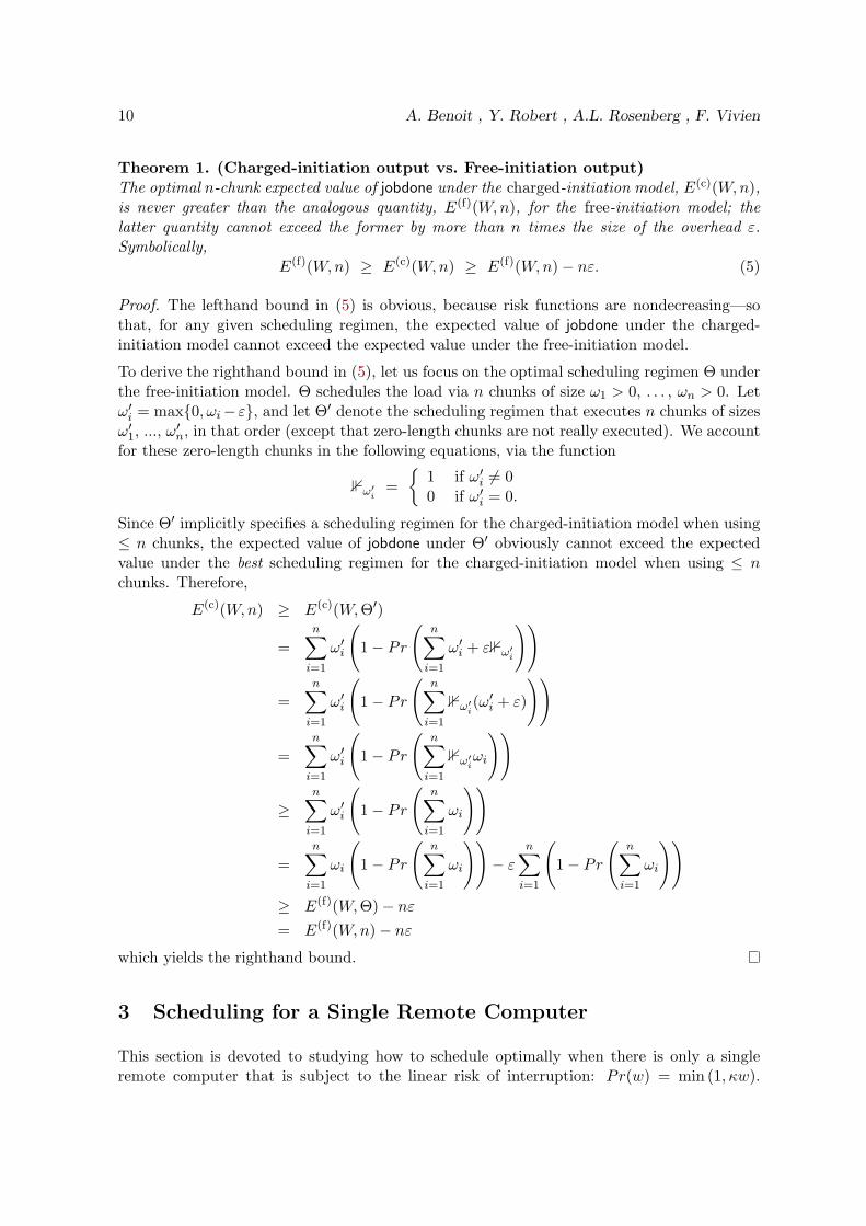
Theorem 1. (Charged-initiation output vs. Free-initiation output)The optimal n-chunk expected value of jobdone under the charged-initiation model, E(c)(W,n),is never greater than the analogous quantity, E(f)(W,n), for the free-initiation model; thelatter quantity cannot exceed the former by more than n times the size of the overhead ε.Symbolically,
E(f)(W,n) ≥ E(c)(W,n) ≥ E(f)(W,n)− nε. (5)
Proof. The lefthand bound in (5) is obvious, because risk functions are nondecreasing—sothat, for any given scheduling regimen, the expected value of jobdone under the charged-initiation model cannot exceed the expected value under the free-initiation model.
To derive the righthand bound in (5), let us focus on the optimal scheduling regimen Θ underthe free-initiation model. Θ schedules the load via n chunks of size ω1 > 0, . . . , ωn > 0. Letω′i = max{0, ωi− ε}, and let Θ′ denote the scheduling regimen that executes n chunks of sizesω′1, ..., ω′n, in that order (except that zero-length chunks are not really executed). We accountfor these zero-length chunks in the following equations, via the function
1ω′i={
1 if ω′i 6= 00 if ω′i = 0.
Since Θ′ implicitly specifies a scheduling regimen for the charged-initiation model when using≤ n chunks, the expected value of jobdone under Θ′ obviously cannot exceed the expectedvalue under the best scheduling regimen for the charged-initiation model when using ≤ nchunks. Therefore,
E(c)(W,n) ≥ E(c)(W,Θ′)
=n∑i=1
ω′i
(1− Pr
(n∑i=1
ω′i + ε1ω′i
))
=n∑i=1
ω′i
(1− Pr
(n∑i=1
1ω′i(ω′i + ε)
))
=n∑i=1
ω′i
(1− Pr
(n∑i=1
1ω′iωi
))
≥n∑i=1
ω′i
(1− Pr
(n∑i=1
ωi
))
=n∑i=1
ωi
(1− Pr
(n∑i=1
ωi
))− ε
n∑i=1
(1− Pr
(n∑i=1
ωi
))≥ E(f)(W,Θ)− nε= E(f)(W,n)− nε
which yields the righthand bound.
3 Scheduling for a Single Remote Computer
This section is devoted to studying how to schedule optimally when there is only a singleremote computer that is subject to the linear risk of interruption: Pr(w) = min (1, κw).

Static Strategies for Worksharing with Unrecoverable Interruptions 11
Some of the results we derive bear a striking similarity to their analogues in [14], despitecertain substantive differences in models.
3.1 An Optimal Schedule under the Free-Initiation Model
We begin with a simple illustration of why the risk of losing work because of an interruptionmust affect our scheduling strategy, even when there is only one remote computer and evenwhen dispatching a new chunk of work incurs no cost, i.e., under the free-initiation model.
When the amount of work W is no larger than X (recall that κ = 1/X is the constant thataccounts for the size of the work-unit), then instantiating the linear risk function, Pr(W ) =κW , in (2) shows that the expected amount of work achieved when deploying the entireworkload in a single chunk is
E(f)(W,Θ1) = W − κW 2.
Similarly, instantiating this risk function in (3) shows that the expected amount of workachieved when deploying the entire workload using two chunks, of respective sizes ω1 > 0 andω2 > 0 is (recalling that ω1 + ω2 = W )
E(f)(W,Θ2) = ω1(1− ω1κ) + ω2(1− (ω1 + ω2)κ))= W − (ω2
1 + ω1ω2 + ω22)κ
= W −W 2κ+ ω1ω2κ.
We observe thatE(f)(W,Θ2)− E(f)(W,Θ1) = ω1ω2κ > 0.
Thus, as one would expect intuitively: For any fixed total workload, one increases the expec-tation of jobdone by deploying the workload as two chunks, rather than one—no matter howone sizes the chunks.
Continuing with the preceding reasoning, we can actually characterize the optimal—i.e.,expectation-maximizing—schedule for any fixed number of chunks. (We thereby also identifya weakness of the free-initiation model: increasing the number of chunks always increasesthe expected amount of work done—so the (unachievable) “optimal” strategy would deployinfinitely many infinitely small chunks.)
Theorem 2. (One remote computer: free-initiation model)Say that one wishes to deploy W ∈ [0, X] units of work to a single remote computer in atmost n chunks, for some positive integer n. In order to maximize the expectation of jobdone,one should have all n chunks share the same size, namely, Z/n units of work, where
Z = min{W,
n
n+ 1X
}.
In expectation, this optimal schedule completes
E(f)(W,n) = Z − n+ 12n
Z2κ
units of work.

12 A. Benoit , Y. Robert , A.L. Rosenberg , F. Vivien
Note that for fixed W , E(f)(W,n) increases with n.
Proof. Let us partition the W -unit workload into n + 1 chunks, of respective sizes ω1 ≥ 0,. . . , ωn ≥ 0, ωn+1 ≥ 0, with the intention of deploying the first n of these chunks.
(a) Our assigning the first n chunks nonnegative, rather than positive sizes affordsus a convenient way to talk about “at most n chunks” using only the single pa-rameter n. (b) By creating n+ 1 chunks rather than n, we allow ourselves to holdback some work in order to avoid what would be a certain interruption of the nthchunk. Formally, exercising this option means making ωn+1 positive; declining theoption—thereby deploying all W units of work—means setting ωn+1 = 0.
Each specific such partition specifies an n-chunk schedule Θn. Our challenge is to choose thesizes of the n + 1 chunks in a way that maximizes E(f)(W,Θn). To simplify notation, letZ = ω1 + · · ·+ ωn denote the portion of the entire workload that we actually deploy.
Extending the reasoning from the cases n = 1 and n = 2, one obtains easily from (4) theexpression
E(f)(W,Θn) = ω1(1− ω1κ) + ω2(1− (ω1 + ω2)κ) + · · ·+ ωn(1− (ω1 + · · ·+ ωn)κ)
= Z − Z2κ +
∑1≤i<j≤n
ωiωj
κ. (6)
Standard arguments show that the bracketed sum in (6) is maximized when all ωi’s share the
common value Z/n, in which case, the sum achieves the value1n2
(n
2
)Z2κ. Since maximizing
the sum also maximizes E(f)(W,Θn), simple arithmetic yields:
E(f)(W,Θn) = Z − n+ 12n
Z2κ.
Viewing this expression for E(f)(W,Θn) as a function of Z, we note that the function isunimodal, increasing until Z =
n
(n+ 1)κand decreasing thereafter. Setting this value for
Z, gives us the maximum value for E(f)(W,Θn), i.e., the value of E(f)(W,n). The theoremfollows.
3.2 An Optimal Schedule under the Charged-Initiation Model
Under the charged-initiation model—i.e., on a computing platform wherein processing a newchunk of work (for transmission or checkpointing) does incur a cost (that we must accountfor)—deriving the optimal strategy becomes dramatically more difficult, even when there isonly one remote computer and even when we know a priori how many chunks we wish toemploy.
Theorem 3. (One remote computer: charged-initiation model)Say that one wishes to deploy W ∈ [0, X] units of work, where X ≥ ε, to a single remote

Static Strategies for Worksharing with Unrecoverable Interruptions 13
computer in at most n chunks, for some positive integer n. Let n1 =⌊
12
(√1 + 8X/ε− 1
)⌋and n2 =
⌊12
(√1 + 8W/ε+ 1
)⌋. The unique regimen for maximizing E(c)(jobdone) specifies
m = min{n, n1, n2} chunks: the first has size7
ω1,m =Z
m+m− 1
2ε
where
Z = min{W,
m
m+ 1X − m
2ε
}; (7)
and the (i+ 1)th chunk inductively has size
ωi+1,m = ωi,m − ε.
In expectation, this schedule completes
E(c)(W,n) = Z − m+ 12m
Z2κ− m+ 12
Zεκ+(m− 1)m(m+ 1)
24ε2κ (8)
units of work.
Proof. We proceed by induction on the number n of chunks we want to partition our W unitsof work into. We denote by E(c)
opt(W,n) the maximum expected amount of work that a schedulecan complete under such a partition.
Focus first on the case n = 1. When work is allocated in a single chunk, the maximumexpected amount of total work completed is, by definition:
E(c)opt(W, 1) = max
0≤ω1,1≤WE(c)(ω1,1) where E(c)(ω1,1) = max
0≤ω1,1≤Wω1,1(1− (ω1,1 + ε)κ).
We determine the optimal size of ω1,1 by viewing this quantity as a variable in the closedinterval [0,W ] and maximizing E(c)(ω1,1) symbolically. We thereby find that E(c)(ω1,1) ismaximized by setting
ω1,1 = min{W,
12κ− ε
2
},
so that
E(c)opt(W, 1) =
1
4κ− ε
2+ε2
4κ if W >
12κ− ε
2,
W −W 2κ−Wεκ otherwise.
(Note that ω1,1 has a non-negative size because of the natural hypothesis that X ≥ ε.)
We now proceed to general values of n by induction. We begin by assuming that the conclu-sions of the theorem have been established for the case when the workload is split into n ≥ 1positive-size chunks. We also assume that n is no greater than min{n1, n2}. In other words,we assume that any optimal solution with at most n chunks used n positive-size chunks.
As our first step in analyzing how best to deploy n+ 1 positive-size chunks, we note that theonly influence the first n chunks of work have on the probability that the last chunk will becomputed successfully is in terms of their cumulative size.
7The second subscript of ω reminds us how many chunks the workload is divided into.

14 A. Benoit , Y. Robert , A.L. Rosenberg , F. Vivien
Let us clarify this last point, which follows from the failure probability model.Denote by An the cumulative size of the first n chunks of work in the expectation-maximizing (n+ 1)-chunk scenario; i.e., An =
∑ni=1 ωi,n+1. Once An is specified,
the probability that the remote computer will be interrupted while working on the(n+ 1)th chunk depends only on the value of An, not on the way the An units ofwork have been divided into chunks.
This fact means that once one has specified the cumulative size of the workload that comprisesthe first n chunks, the best way to partition this workload into chunks is as though it werethe only work in the system, i.e., as if there were no (n + 1)th chunk to be allocated. Thus,one can express Eopt(W,n + 1) in terms of An (whose value must, of course, be determined)and Eopt(An, n), via the following maximization.
Eopt(W,n+ 1) = max{Eopt(An, n) + ωn+1,n+1 (1− (An + ωn+1,n+1 + (n+ 1)ε)κ)
},
where the maximization is over all values for An in which
An > 0 allowing for the n previous chunksωn+1,n+1 ≥ 0 allowing for an (n+ 1)th chunk
An + ωn+1,n+1 ≤ W because the total workload has size WAn + ωn+1,n+1 + (n+ 1)ε ≤ X reflecting the risk and cost models
The last of these inequalities acknowledges that the remote computer is certain to be inter-rupted (with probability 1) before it can complete the (n+ 1)th chunk of work, if its overallworkload is no smaller than X − (n+ 1)ε.
We now have two cases to consider, depending on the size of An.
Case 1: An <n
n+ 1X − n
2ε.
By assumption, the expectation-maximizing regimen deploys An units of work via its first nchunks. By induction, expression (8) tells us that the expected amount of work completed bydeploying these An units is
E(c)opt(An, n) = An −
n+ 12n
A2nκ−
n+ 12
Anεκ+(n− 1)n(n+ 1)
24ε2κ.
Let Z denote the total work that is actually allocated: Z = An + ωn+1,n+1. In the followingcalculations, we write ωn+1,n+1 as Z − An, in order to represent the (n + 1)-chunk scenarioentirely via quantities that arise in the n-chunk scenario.
We focus on
E(1)(An, ωn+1,n+1) = Eopt(An, n) + (Z −An) (1− (Z + (n+ 1)ε)κ)
=(An −
n+ 12n
A2nκ−
n+ 12
Anεκ+(n− 1)n(n+ 1)
24ε2κ
)+ (Z −An) (1− (Z + (n+ 1)ε)κ)
=(Z +
n+ 12
ε
)Anκ−
n+ 12n
A2nκ
+ Z(1− (Z + (n+ 1)ε)κ) +(n− 1)n(n+ 1)
24ε2κ.

Static Strategies for Worksharing with Unrecoverable Interruptions 15
For a given value of Z, we look for the best value for An using the preceding expression. Wenote first that
∂E(1)(An, ωn+1,n+1)∂An
= −n+ 1n
Anκ+ Zκ+n+ 1
2εκ.
We note next that, for fixed Z, the quantity E(1)(An, ωn+1,n+1) begins to increase with An andthen decreases. The value for An that maximizes this expectation, which we denote A(opt)
n , is
A(opt)n = min
{W,
n
n+ 1Z +
n
2ε
}.
When W ≤ (n/(n+ 1))Z+ 12nε, A
(opt)n = W , meaning that the (n+ 1)th chunk is empty, and
the schedule does not optimize the expected work. (In the charged-initiation model an emptychunk decreases the overall probability). Consequently, we focus for the moment on the case
A(opt)n =
n
n+ 1Z +
n
2ε (9)
(thereby assuming that W ≥ (n/(n+ 1))Z + 12nε). Therefore, we have
E(1)(A(opt)n , ωn+1,n+1) = − n+ 2
2(n+ 1)Z2κ+ Z − n+ 2
2εZκ+
n(n+ 1)(n+ 2)24
ε2κ.
We maximize E(1)(A(opt)n , ωn+1,n+1) via the preceding expression by viewing the expectation
as a function of Z. We discover that E(1)(A(opt)n , ωn+1,n+1) is maximized when
Z = Z(opt) = min{n+ 1n+ 2
X − n+ 12
ε, W
}. (10)
For this case to be meaningful, the (n + 1)th chunk must be nonempty, so that A(opt)n < Z;
i.e., Z > 12n(n+ 1)ε. Therefore, we must simultaneously have:
1. (n+1)/(n+2)X− 12(n+1)ε > 1
2n(n+1)ε, so that X > 12(n+1)(n+2)ε, which requires
that n ≤⌊
12
(√1 + 8X/ε− 3
)⌋.
2. W > 12n(n+ 1)ε, which requires that n ≤
⌊12
(√1 + 8W/ε− 1
)⌋.
We can now check the sanity of the result.
Z(opt) + (n+ 1)ε ≤ n+ 1n+ 2
X − n+ 12
ε+ (n+ 1)ε < X,
because of the just established condition 12(n+ 1)(n+ 2)ε < X. We also have,
A(opt)n =
n
n+ 1Z +
n
2ε ≤ n
n+ 1
(n+ 1n+ 2
X − n+ 12
ε
)+n
2ε =
n
n+ 2X <
n
n+ 1X − n
2ε
because 12(n+1)(n+2)ε < X. Therefore, the solution is consistent with the defining hypothesis
for this case—namely, that An <n
n+ 1X − n
2ε.

16 A. Benoit , Y. Robert , A.L. Rosenberg , F. Vivien
Before moving on to case 2, we note that the value (9) does, indeed, extend our inductivehypothesis. To wit, the optimal total amount of allocated work, Z(opt), has precisely thepredicted value, and the sizes of the first n chunks do follow a decreasing arithmetic progressionwith common difference ε (by using the induction hypothesis). Finally, the last chunk hasthe claimed size:
ωn+1,n+1 = Z(opt) −A(opt)n =
1n+ 1
Z(opt) − n
2ε.
We turn now to our remaining chores. We must derive the expectation-maximizing chunk sizesfor the second case, wherein An is “big.” And, we must show that the maximal expected workcompletion in this second case is always dominated by the solution of the first case—whichwill lead us to conclude that the regimen of the theorem is, indeed, optimal.
Case 2: An ≥n
n+ 1X − n
2ε.
By (7), if the current case’s restriction on An is an inequality, then An cannot be an optimalcumulative n-chunk work allocation. We lose no generality, therefore, by focusing only on thesubcase when the defining restriction of An is an equality:
An =n
n+ 1X − n
2ε.
For this value of An, call it A?n, we have
Eopt(W,n+ 1) = max(Eopt(A?n, n) + ωn+1,n+1 (1− (A?n + ωn+1,n+1 + (n+ 1)ε)κ)
),
where the maximization is over all values of ωn+1,n+1 in the closed interval [0, W −A?n].
To determine a value of ωn+1,n+1 that maximizes Eopt(W,n + 1) for A?n, we focus on thefunction
E(2)(An, ωn+1,n+1) = Eopt(An, n) + ωn+1,n+1 (1− (An + ωn+1,n+1 + (n+ 1)ε)κ)
=(An −
n+ 12n
A2nκ−
n+ 12
Anεκ+(n− 1)n(n+ 1)
24ε2κ
)+ ωn+1,n+1 (1− (An + ωn+1,n+1 + (n+ 1)ε)κ)
= −κω2n+1,n+1 +
(−n+ 2
2κε+
1n+ 1
)ωn+1,n+1
+n((n+ 1)2(n+ 2)ε2κ2 − 12(n+ 1)εκ+ 12
)24(n+ 1)κ
.
Easily,∂E(2)(An, ωn+1,n+1)
∂ωn+1,n+1= −2κωn+1,n+1 −
n+ 22
κε+1
n+ 1.
Knowing A?n exactly, we infer that the value of ωn+1,n+1 that maximizes E(2)(A?n, ωn+1,n+1) is
ωn+1,n+1 = min{
12(n+ 1)
X − 14
(n+ 2)ε, W − n
n+ 1X − n
2ε
}.
The second term dominates this minimization whenever
W ≥ 2n+ 12n+ 2
X +n− 2
4ε;

Static Strategies for Worksharing with Unrecoverable Interruptions 17
therefore, if W is large enough—as delimited by the preceding inequality—then
E(2)(A?n, ωn+1,n+1) =2n2 + 2n+ 1
4(n+ 1)2X − 2n2 + 3n+ 2
4(n+ 1)ε+
(n+ 2)(2n2 + 5n+ 648
κε2,
When W does not achieve this threshold, then
E(2)(A?n, ωn+1,n+1) =−W 2κ+(n− 2
2κε+
2n+ 1n+ 1
)W
+(n2 + 3n+ 14)nκε2
24− n2
n+ 1ε− n
2(n+ 1)X.
For the found solution to be meaningful, the (n + 1)th chunk must be nonempty, i.e.,ωn+1,n+1 > 0. This has two implications.
1. X > (n+1)(n+2)2 ε, which is true as long as n ≤
⌊12
(√1 + 8X/ε− 3
)⌋.
2. W − (n/(n + 1))X − 12nε > 0, which implies W > 1
2n(n + 1)ε because X ≥ W . This
inequality on W is true as long as n ≤⌊
12
(√1 + 8W/ε− 1
)⌋.
Because X > 12(n+ 1)(n+ 2)ε, we have
An + ωn+1,n+1 + (n+ 1)ε ≤ n
n+ 1X − n
2ε+
12(n+ 1)κ
− 14
(n+ 2)ε+ (n+ 1)ε ≤ X.
For both Case 1 and Case 2, if either condition[n ≤
⌊12
(√1 + 8X/ε− 3
)⌋]or
[n ≤
⌊12
(√1 + 8W/ε− 1
)⌋]does not hold, then there is no optimal schedule with (n + 1) nonempty chunks. (We willcome back later to the case where one of these conditions does not hold.) If both conditionshold, then Case 1 always has an optimal schedule, but Case 2 may not have one.
To complete the proof, we must verify that the optimal regimen always corresponds to Case 1(as suggested by the theorem), never to Case 2 (whenever Case 2 defines a valid solution).We accomplish this by considering two cases, depending on the size W of the workload. Weshow that the expected work completed under the regimen of Case 1 is never less than underthe regimen of Case 2.
Case A: W ≥ n+ 1n+ 2
X − n+ 12
ε.
Under this hypothesis, and under Case 1, the workload that is actually deployed has size
Z =n+ 1n+ 2
X − n+ 12
ε,
so that, in expectation,
E(1)(W,n+ 1) = Z − n+ 12n
Z2κ− n+ 12
Zεκ+(n− 1)n(n+ 1)
24ε2κ
=n+ 1
2(n+ 2)X − n+ 1
2ε+
(n+ 1)(n+ 2)(n+ 3)24
ε2κ.

18 A. Benoit , Y. Robert , A.L. Rosenberg , F. Vivien
units of work are completed. Moreover, because
n+ 1n+ 2
X − n+ 12
ε ≤ 2n+ 12n+ 2
X +n− 2
4ε,
the most favorable value for E(1)(W,n + 1) under Case 2 lies within the range of values forthe current case. Because the value of E(1)(W,n+ 1) is constant whenever
W ≥ n+ 1n+ 2
X − n+ 12
ε,
we can reach the desired conclusion by just showing that this value is no smaller than
E(2)
(2n+ 12n+ 2
X +n− 2
4ε, n+ 1
). Thus, we need only focus on the specific value
Wlim =2n+ 12n+ 2
X +n− 2
4ε
for W . For this value, we have:
E(2)(Wlim, n+ 1) = −W 2limκ+
(n− 2
2κε+
2n+ 1n+ 1
)Wlim +
(n2 + 3n+ 14)nκε2
24
− n2
n+ 1ε− n
2(n+ 1)X
=2n2 + 2n+ 1
4(n+ 1)2X − 2n2 + 3n+ 2
4(n+ 1)ε+
(n+ 2)(2n2 + 5n+ 6)48
ε2κ.
By explicit calculation, we finally see that
E(1)(W,n+ 1)− E(2)(Wlim, n+ 1) =
(4 + (n4 + 6n3 + 13n2 + 12n+ 4)κ2ε2
)n
16(n+ 1)2(n+ 2)κ
− (4n2 + 12n+ 8)κεn16(n+ 1)2(n+ 2)κ
=
(4 + (n+ 1)2(n+ 2)2κ2ε2 − 4(n+ 1)(n+ 2)κε
)n
16(n+ 1)2(n+ 2)κ
=((n+ 1)(n+ 2)κε− 2)2 n
16(n+ 1)2(n+ 2)κ≥ 0.
Case B: W ≤ n+ 1n+ 2
X − n+ 12
ε.
In this case, the regimen of Case 1 deploys all W units of work, thereby completing, inexpectation,
E(1)(W,n+ 1) = W − n+ 12n
W 2κ− n+ 12
Wεκ+(n− 1)n(n+ 1)
24ε2κ.
units of work. Moreover,
n+ 1n+ 2
X − n+ 12
ε ≤ 2n+ 12n+ 2
X +n− 2
4ε,

Static Strategies for Worksharing with Unrecoverable Interruptions 19
so that the regimen of Case 2 also deploys all W units of work, thereby completing, inexpectation,
E(2)(W,n+ 1) =−W 2κ+(n− 2
2κε+
2n+ 1n+ 1
)W
+(n2 + 3n+ 14)nκε2
24− n2
n+ 1ε− n
2(n+ 1)X.
units of work.
Explicit calculation now shows that
E(1)(W,n+ 1)− E(2)(W,n+ 1) =n
2(n+ 1)W 2κ− n
n+ 1(1 + (n+ 1)εκ)W
+n
2(n+ 1)(1 + 2nκε− (n+ 1)κ2ε2)X.
Viewed as a function of W , this difference is, thus, unimodal, decreasing up to its globalminimum, which occurs at W = X + (n+ 1)ε, and increasing thereafter. The largest value ofW allowed by the current case is
Wmax =n+ 1n+ 2
X − n+ 12
ε,
so this is also the value on which the difference E(1)(W,n + 1) − E(2)(W,n + 1) reaches itsminimum within its domain of validity. Thus, we need only focus on the behavior of thedifference at the value W = Wmax. At this value,
E(1)(Wmax, n+ 1)− E(2)(Wmax, n+ 1) =n(5n+ 1)ε2κ
8+
(n− 1)nε2(n+ 1)(n+ 2)
+n
2(n+ 1)(n+ 2)2κ.
This quantity is obviously positive, which means that E(1)(Wmax, n+ 1) > E(2)(Wmax, n+ 1).
We thus see that, for workloads of any size W , one completes at least as much expected workvia the schedule of Case 1 as via the schedule of Case 2.
In summation, if
n ≤ min{⌊
12
(√1 + 8X/ε− 3
)⌋,
⌊12
(√1 + 8W/ε− 1
)⌋}, (11)
then Case 1 specifies the optimal schedule that uses no more than n + 1 chunks. Of course,this inequality translates to the conditions of the theorem (where it is written for n chunksinstead of n+ 1).
Note that if n exceeds either quantity in the minimization of (11), then one never improvesthe expected amount of work completed by deploying the workload in more than n chunks.This is another consequence of our remark about An at the beginning of this proof. If thereexists a value of m for which there exists a schedule S that uses ≥ n + 1 nonempty chunks,then replacing the first n+ 1 chunks in this solution with the optimal solution for n chunks,using a workload equal to the first n+ 1 chunks of S, yields a schedule that, in expectation,completes strictly more work than S.

20 A. Benoit , Y. Robert , A.L. Rosenberg , F. Vivien
4 Scheduling for Two Remote Computers
Before we approach the general case of p remote computers, we study the case of two remotecomputers, in order to adduce principles that will be useful in the general case. We first estab-lish characteristics of optimal schedules under general risk functions, then restrict attentionto the linear risk model. Throughout this section, we consider two remote computers, P1 andP2, under the free-initiation model.
4.1 Two Remote Computers under General Risk
Focus on a distribution of work to P1 and P2 under which, for i = 1, 2, Pi receives ni chunksto execute, call them Wi,1, . . . , Wi,ni , to be scheduled in this order; as usual we denote |Wi,j |by ωi,j . We do not assume any a priori relation between the way P1 and P2 break theirallocated work into chunks; in particular, any work that is allocated to both P1 and P2 maybe chunked quite differently on the two machines.
Theorem 4. (Two remote computers: free-initiation model; general risk)Let Θ be a schedule for two remote computers, P1 and P2. Say that, for both P1 and P2, theprobability of being interrupted never decreases as a computer processes more work. Thereexists a schedule Θ′ for P1 and P2 that, in expectation, completes as much work as does Θand that satisfies the following three properties; cf. Fig. 1.
Maximal work deployment. Θ′ deploys as much of the overall workload as possible. There-fore, the workloads it deploys to P1 and P2 can overlap only if their union is the entireoverall workload.
Local work priority. Θ′ has P1 (resp., P2) process all of the allocated work that it does notshare with P2 (resp., P1) before it processes any shared work.
Shared work “mirroring.” Θ′ has P1 and P2 process their shared work “in opposite orders.”Specifically, say that P1 chops its allocated work into chunks W1,1, . . . ,W1,n1, while P2
chops its allocated work into chunks W2,1, . . . ,W2,n2.
Say that there exist chunk-indices a1, b1 > a1 for P1, and a2, b2 > a2 for P2 such that:chunks W1,a1 and W2,a2 both contain a shared “piece of work”A, and chunks W1,b1 andW2,b2 both contain a shared “piece of work” B.
Then if Θ′ has P1 execute A before B (i.e., P1 executes chunkW1,a1 before chunkW1,b1),then Θ′ has P2 execute B before A (i.e., P2 executes chunk W2,b2 before chunk W2,a2).
Proof. We need to refine our description of workloads. We describe the overall workload ofsize W via a partition X = {X1, ...,Xm} such that, for j = 1, 2, each element Xi ∈ X is eitherincluded in a chunk of Pj or does not intersect any chunk of Pj . Symbolically:
(∀i ∈ [1..m])
[Xi ∩
n1⋃k=1
Wj,k = ∅
]OR (∃k ∈ [1..n1]) [Xi ⊂ Wj,k] .

Static Strategies for Worksharing with Unrecoverable Interruptions 21
W1,2 W1,3
W2,3 W2,2 W2,1
W1,1
Figure 1: The shape of an optimal schedule for two computers, as described in Theorem 4;n1 = n2 = 3. The top row displays P1’s chunks, the bottom row P2’s. Vertically aligned partsof chunks correspond to shared work; shaded areas depict unallocated work (e.g., none of thework in W2,1 is allocated to P1).
We then define, for j = 1, 2 and i = 1, . . . nj ,
δj(i) ={
0 just when element Xi ∈ X does not intersect any chunk of Pj1 otherwise.
When δj(i) = 1, we denote by σj(i) the chunk of Pj that contains Xi, so that Xi ⊂ Wj,σj(i).
We can now specify the expectation E of jobdone under the described distribution of chunksto P1 and P2. The probability that element Xi ∈ X is computed successfully is:
• 0 if Xi is not allocated to either P1 or P2;
• 1− Pr(∑σ1(i)
j=1 ω1,j
)if Xi is allocated to P1 but not to P2, i.e., if δ1(i)(1− δ2(i)) = 1;
• 1− Pr(∑σ2(i)
j=1 ω2,j
)if Xi is allocated to P2 but not to P1, i.e., if (1− δ1(i))δ2(i) = 1;
• 1 − Pr(∑σ1(i)
j=1 ω1,j
)Pr(∑σ2(i)
j=1 ω2,j
)if Xi is allocated to both P1 and P2, i.e., if
δ1(i)δ2(i) = 1.
We thus end up with the following overall expression for E , the expected amount of workcompleted under the described distribution:
E =m∑i=1
|Xi| · Ξi,
where
Ξi = δ1(i)δ2(i)
1− Pr
σ1(i)∑j=1
ω1,j
Pr
σ2(i)∑j=1
ω2,j
+ δ1(i)(1− δ2(i))
1− Pr
σ1(i)∑j=1
ω1,j
+ (1− δ1(i))δ2(i)
1− Pr
σ2(i)∑j=1
ω2,j
.
22 A. Benoit , Y. Robert , A.L. Rosenberg , F. Vivien
We now verify the existence of an optimal schedule Θ that satisfies each of the three claimedproperties. In fact, we prove a slightly stronger claim, by verifying these properties of Θ forthe partition elements rather than for the chunks.
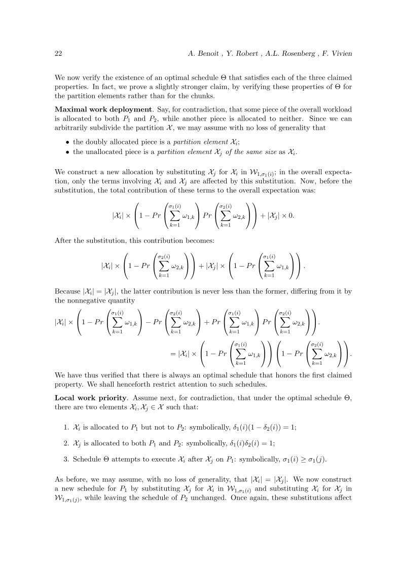
Maximal work deployment. Say, for contradiction, that some piece of the overall workloadis allocated to both P1 and P2, while another piece is allocated to neither. Since we canarbitrarily subdivide the partition X , we may assume with no loss of generality that
• the doubly allocated piece is a partition element Xi;• the unallocated piece is a partition element Xj of the same size as Xi.
We construct a new allocation by substituting Xj for Xi in W1,σ1(i); in the overall expecta-tion, only the terms involving Xi and Xj are affected by this substitution. Now, before thesubstitution, the total contribution of these terms to the overall expectation was:
|Xi| ×
1− Pr
σ1(i)∑k=1
ω1,k
Pr
σ2(i)∑k=1
ω2,k
+ |Xj | × 0.
After the substitution, this contribution becomes:
|Xi| ×
1− Pr
σ2(i)∑k=1
ω2,k
+ |Xj | ×
1− Pr
σ1(i)∑k=1
ω1,k
.
Because |Xi| = |Xj |, the latter contribution is never less than the former, differing from it bythe nonnegative quantity
|Xi| ×
1− Pr
σ1(i)∑k=1
ω1,k
− Prσ2(i)∑k=1
ω2,k
+ Pr
σ1(i)∑k=1
ω1,k
Pr
σ2(i)∑k=1
ω2,k
.
= |Xi| ×
1− Pr
σ1(i)∑k=1
ω1,k
1− Pr
σ2(i)∑k=1
ω2,k
.
We have thus verified that there is always an optimal schedule that honors the first claimedproperty. We shall henceforth restrict attention to such schedules.
Local work priority. Assume next, for contradiction, that under the optimal schedule Θ,there are two elements Xi,Xj ∈ X such that:
1. Xi is allocated to P1 but not to P2: symbolically, δ1(i)(1− δ2(i)) = 1;
2. Xj is allocated to both P1 and P2: symbolically, δ1(i)δ2(i) = 1;
3. Schedule Θ attempts to execute Xi after Xj on P1: symbolically, σ1(i) ≥ σ1(j).
As before, we may assume, with no loss of generality, that |Xi| = |Xj |. We now constructa new schedule for P1 by substituting Xj for Xi in W1,σ1(i) and substituting Xi for Xj inW1,σ1(j), while leaving the schedule of P2 unchanged. Once again, these substitutions affect

Static Strategies for Worksharing with Unrecoverable Interruptions 23
only the terms involving Xi and Xj in the overall expectation. The total contribution of theseterms before the substitution was:
|Xi| ×
1− Pr
σ1(i)∑k=1
ω1,k
+ |Xj | ×
1− Pr
σ1(j)∑k=1
ω1,k
Pr
σ2(j)∑k=1
ω2,k
.
After the substitution, the contribution becomes
|Xi| ×
1− Pr
σ1(j)∑k=1
ω1,k
+ |Xj | ×
1− Pr
σ1(i)∑k=1
ω1,k
Pr
σ2(j)∑k=1
ω2,k
.
Because |Xi| = |Xj |, we see that the substitution increases the overall expectation by thequantity
|Xi| ×
Prσ1(i)∑k=1
ω1,k
− Prσ1(j)∑
k=1
ω1,k
×1− Pr
σ2(j)∑k=1
ω2,k
,
This quantity is nonnegative because
• the probability Pr(w) is nondecreasing in w;•∑σ1(i)
k=1 ω1,k ≥∑σ1(j)
k=1 ω1,k, because σ1(i) ≥ σ1(j).
The modified schedule completes, in expectation, at least as much work as Θ, and it satisfiesthe second property.
Shared work “mirroring.” Finally, consider a schedule under which there are two partitionelements, Xi and Xj , such that:
1. Both Xi and Xj are allocated to both P1 and P2: symbolically, δ1(i)δ2(i) = δ1(j)δ2(j) =1;
2. The optimal schedule Θ attempts to execute Xi after Xj on both P1 and P2: symbolically,[σ1(i) ≥ σ1(j)] and [σ2(i) ≥ σ2(j)].
As before, we may assume with no loss of generality that the |Xi| = |Xj |. We now construct anew schedule by substituting Xj for Xi inW1,σ1(i) and substituting Xi to Xj inW1,σ1(j), leavingthe schedule of P2 unchanged. Once again, these changes affect only the terms involving Xiand Xj in the overall expectation. The total contribution of these terms before the substitutionwas:
|Xi|×
1− Pr
σ1(i)∑k=1
ω1,k
Pr
σ2(i)∑k=1
ω2,k
+|Xj |×
1− Pr
σ1(j)∑k=1
ω1,k
Pr
σ2(j)∑k=1
ω2,k
.
After the substitution, their contribution becomes:
|Xi|×
1− Pr
σ1(j)∑k=1
ω1,k
Pr
σ2(i)∑k=1
ω2,k
+|Xj |×
1− Pr
σ1(i)∑k=1
ω1,k
Pr
σ2(j)∑k=1
ω2,k
.

24 A. Benoit , Y. Robert , A.L. Rosenberg , F. Vivien
Because |Xi| = |Xj |, the substitutions have increased the overall expectation by the quantity:
|Xi| ×
Prσ1(j)∑
k=1
ω1,k
− Prσ1(i)∑k=1
ω1,k
Prσ2(j)∑
k=1
ω2,k
− Prσ2(i)∑k=1
ω2,k
.
This quantity is nonnegative because Xi and Xj are processed in the same order on P1 andon P2. The modified schedule thus completes, in expectation, at least as much work as Θ,and it satisfies the third property.
4.2 Two Remote Computers under Linear Risk
4.2.1 Allocating work in a single chunk
We now specialize from general risk functions to the linear risk functions. We first considerthe case wherein each computer processes its allocated work as a single chunk. Even thissimple case turns out to be surprisingly difficult to schedule optimally when there is morethan one remote computer. Indeed, our experience with this case leads us to abandon thequest for exactly optimal schedules, in favor of the more easily accessed asymptotically optimalschedules.
“Asymptotically optimal”here means that the expected amount of work completedby these schedules deviates from exact maximality by an amount that shrinks asthe size of the workload grows without bound.
To render the single-chunk scheduling problem tractable, we restrict attention to schedulesthat are symmetric, in the sense that they allocate the same amount of work to each remotecomputer. It seems intuitive that there is always a symmetric schedule among the optimalsingle-chunk schedules, but we have yet to verify this.
Say that our workload consists of W units of work that we somehow order linearly. We denoteby 〈a, b〉 the sub-workload obtained by eliminating: the initial a units of work and all workbeyond the initial b units. For instance, 〈0,W 〉 denotes the entire workload, 〈0, 1
2W 〉 denotesthe first half of the workload, and 〈12W,W 〉 denotes the last half of the workload.
Theorem 5. (Two remote computers: linear risk; single chunk allocation)Say that we wish to deploy W units of work on two computers, deploying a single chunk percomputer. The following symmetric schedule Θ completes, in expectation, a maximum amountof work.
• If W ≤ 12X, then Θ deploys the entire workload on both remote computers; symbolically,
W1,1 =W2,1 = 〈0,W 〉;
• if 12X < W ≤ X, then Θ deploys the first half of the workload on one computer and the
second half on the other; symbolically, W1,1 = 〈0, 12W 〉, and W2,1 = 〈12W,W 〉;
• if X < W , then Θ deploys only X units of the workload, allocating the first half to onecomputer and the second half to the other; symbolically, W1,1 = 〈0, 1
2X〉, and W2,1 =〈12X,X〉.

Static Strategies for Worksharing with Unrecoverable Interruptions 25
Proof. Our derivation of the optimal schedule builds on the following principle (which we haveencountered before). When we deploy work as a single chunk, we never make that chunk aslarge as X, for then we risk certain interruption, hence, in expectation, completes no work. Inorder to see how to optimally deploy work as a single chunk, we consider separately schedulesthat allow overlapping deployments to the two computers and those that do not.
Disjoint allocations. Focus first on schedules that deploy non-overlapping workloads tothe two remote computers. These two workloads, W1,1 and W2,1, are independent, so wecan invoke Theorem 2 to discover their optimal sizes. We see that the optimal strategy isto deploy Z = min{W,X} units of work in total. We determine the optimal allocation ofthis work to the remote computers, in respective chunk sizes ω1,1 and ω2,1 = Z − ω1,1, byconsidering the expectation of jobdone.
E = ω1,1 ((1− ω1,1κ) + (Z − ω1,1)(1− (Z − ω1,1)κ))= −2ω2
1,1κ+ 2ω1,1Zκ+ Z − Z2κ.,
Easily, E is maximized when ω1,1 = ω2,1 = 12Z. The optimal value of E is, then, E = W− 1
2Z2κ.
(Note that we did not need to assume that the optimal schedule is symmetric in this case; weactually proved that it should be.)
Overlapping allocations to the two computers. The principle enunciated at the begin-ning of this proof implies that an optimal schedule that deploys overlapping workloads to thetwo remote computers never allocates a full X units of work to either computer. We can,therefore, simplify our calculations by restricting attention henceforth to the case W < 2X.Since we consider only symmetric schedules, the common size s of the allocations to bothcomputers satisfies s ≥ W
2 , by Theorem 4. We thus obtain the following expression for theexpectation of jobdone as a function of s.
E(s) = 2(W − s)(1− sκ) + (2s−W )(1− s2κ2)= −2s3κ2 + (2 +Wκ)s2κ− 2sWκ+W.
We seek the maximizing value of s.
E ′(s) =ddsE(s) = 2[−3s2κ+ (2 +Wκ)s−W ]κ.
The discriminant of the bracketed quadratic polynomial is
∆ = W 2κ2 − 8Wκ+ 4 = (Wκ− 2(2 +√
3))(Wκ− 2(2−√
3)).
Because W < 2X we have, Wκ < 2(2 +√
3). We branch on the relative sizes of W and2(2−
√3)X:
W > 2(2−√
3)X. In this case, ∆ < 0, so the polynomial has no real roots, and E(s) isdecreasing with s. Because s ∈ [1
2W,W ], E(s) is maximized when s = W/2.
W ≤ 2(2−√
3)X. This case is far more complicated than its predecessor. Let us denote thetwo roots of our quadratic polynomial by s− and s+, as follows:
s− =2 +Wκ−
√W 2κ2 − 8Wκ+ 4
6κand s+ =
2 +Wκ+√W 2κ2 − 8Wκ+ 4
6κ.
26 A. Benoit , Y. Robert , A.L. Rosenberg , F. Vivien
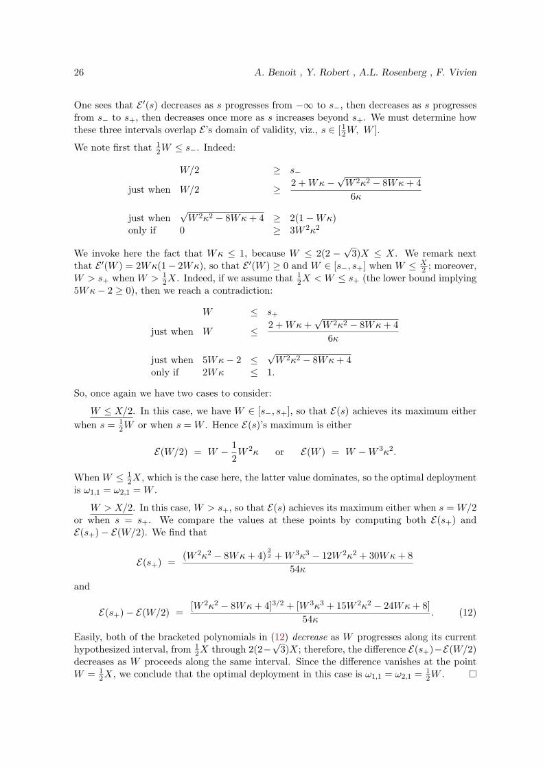
One sees that E ′(s) decreases as s progresses from −∞ to s−, then decreases as s progressesfrom s− to s+, then decreases once more as s increases beyond s+. We must determine howthese three intervals overlap E ’s domain of validity, viz., s ∈ [1
2W, W ].
We note first that 12W ≤ s−. Indeed:
W/2 ≥ s−
just when W/2 ≥ 2 +Wκ−√W 2κ2 − 8Wκ+ 4
6κ
just when√W 2κ2 − 8Wκ+ 4 ≥ 2(1−Wκ)
only if 0 ≥ 3W 2κ2
We invoke here the fact that Wκ ≤ 1, because W ≤ 2(2 −√
3)X ≤ X. We remark nextthat E ′(W ) = 2Wκ(1− 2Wκ), so that E ′(W ) ≥ 0 and W ∈ [s−, s+] when W ≤ X
2 ; moreover,W > s+ when W > 1
2X. Indeed, if we assume that 12X < W ≤ s+ (the lower bound implying
5Wκ− 2 ≥ 0), then we reach a contradiction:
W ≤ s+
just when W ≤ 2 +Wκ+√W 2κ2 − 8Wκ+ 4
6κ
just when 5Wκ− 2 ≤√W 2κ2 − 8Wκ+ 4
only if 2Wκ ≤ 1.
So, once again we have two cases to consider:
W ≤ X/2. In this case, we have W ∈ [s−, s+], so that E(s) achieves its maximum eitherwhen s = 1
2W or when s = W . Hence E(s)’s maximum is either
E(W/2) = W − 12W 2κ or E(W ) = W −W 3κ2.
When W ≤ 12X, which is the case here, the latter value dominates, so the optimal deployment
is ω1,1 = ω2,1 = W .
W > X/2. In this case, W > s+, so that E(s) achieves its maximum either when s = W/2or when s = s+. We compare the values at these points by computing both E(s+) andE(s+)− E(W/2). We find that
E(s+) =(W 2κ2 − 8Wκ+ 4)
32 +W 3κ3 − 12W 2κ2 + 30Wκ+ 8
54κ
and
E(s+)− E(W/2) =[W 2κ2 − 8Wκ+ 4]3/2 + [W 3κ3 + 15W 2κ2 − 24Wκ+ 8]
54κ. (12)
Easily, both of the bracketed polynomials in (12) decrease as W progresses along its currenthypothesized interval, from 1
2X through 2(2−√
3)X; therefore, the difference E(s+)−E(W/2)decreases as W proceeds along the same interval. Since the difference vanishes at the pointW = 1
2X, we conclude that the optimal deployment in this case is ω1,1 = ω2,1 = 12W .

Static Strategies for Worksharing with Unrecoverable Interruptions 27
Moving beyond Theorem 5. The preceding analysis determines the optimal schedulefor only two remote computers that each process their allocations as single chunks. Thecomplexity of even this simple case has led us to abandon our focus on exactly optimalschedules in the sequel, in favor of a hopefully more tractable search for schedules that areasymptotically optimal.
Since one can view schedules under the free-initiation model as “asymptotic ver-sions” of schedules under the charged-initiation model—cf. Theorem 1—our shiftin focus is not a drastic one.
This shift in focus notwithstanding, it is worth seeking significant restricted situations whereinone can tractably discover exactly optimal schedules. One obvious candidate for specialconsideration is the family of schedules that allocate the entire workload to each remotecomputer—which seems to be desirable when Wκ is small enough. We conjecture that, forsuch schedules, an optimal strategy would have the two computers chop the workload intochunks of the same size and then process these chunks in “opposite orders” (as defined in thethird property of Theorem 4). When all remote computers chop the workload into n chunks,this scheduling strategy completes, in expectation,
E = W − W 3κ2
6
(1 +
3n
+2n2
)units of work (cf. Theorem 6 below). Extensive numerical simulations suggest that such ascheduling strategy is, indeed, optimal as long as n ≤ 3. However, we know that the strategyis suboptimal once one allows n to exceed 3. Indeed, for n = 4, the strategy completes, inexpectation, W − 5
16W3κ2 units of work, which is strictly less than the W − 757−73
√73
432 W 3κ2
units completed, in expectation, by the strategy specified schematically in Fig. 2 (with m = 1and α =
√73−76 W ).
The boxes in Figs. 2 and 3 contain chunk sizes. In Fig. 2, for instance, eachcomputer uses m chunks of size α, two chunks of size 1
4(W −mα), and one chunkof size 1
2(W −mα).
Furthermore, the schedule in Fig. 2 is suboptimal as soon as we allow computers to chop workinto eight chunks. To wit, Fig. 3 presents an 8-chunk schedule that completes, in expectation,W − 229−44
√22
98 W 3κ2 ≈ W − 0.230834W 3κ2 units of work, when α = 4√
22−1714 W , while the
schedule of Fig. 2, using 8 chunks per computer (specifically, m = 5 and α = 19−√
19342 W )
completes, in expectation, W − 18293−965√
19321168 W 3κ2 ≈ W − 0.230857W 3κ2 units of work.
(The schedule of Fig. 3 is not even optimal for 8 chunks, but the best schedule we foundnumerically was almost identical but slightly less regular.)
The increasing complexities of the preceding “counterexample” schedules suggest how hardit will be to search for, and characterize, exactly optimal schedules—even in the presence ofsimplifying assumptions, such as that the whole workload is distributed to each computer.Since our simulations suggest that simple regular solutions often complete, in expectation,almost as much work as do complex exactly optimal schedules, we henceforth aim for simplystructured asymptotically optimal schedules.
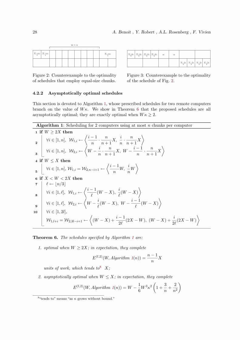
28 A. Benoit , Y. Robert , A.L. Rosenberg , F. Vivien
m× α
W−mα4
W−mα2
W−mα4
Figure 2: Counterexample to the optimalityof schedules that employ equal-size chunks.
W−2α8
W−2α8
W−2α8
W−2α8
W−2α8
W−2α8
W−2α8
W−2α8
α α
Figure 3: Counterexample to the optimalityof the schedule of Fig. 2.
4.2.2 Asymptotically optimal schedules
This section is devoted to Algorithm 1, whose prescribed schedules for two remote computersbranch on the value of Wκ. We show in Theorem 6 that the proposed schedules are allasymptotically optimal; they are exactly optimal when Wκ ≥ 2.
Algorithm 1: Scheduling for 2 computers using at most n chunks per computerif W ≥ 2X then1
∀i ∈ [1, n], W1,i ←⟨i− 1n· n
n+ 1X,
i
n· n
n+ 1X
⟩2
∀i ∈ [1, n], W2,i ←⟨W − i
n· n
n+ 1X, W − i− 1
n· n
n+ 1X
⟩3
if W ≤ X then4
∀i ∈ [1, n], W1,i =W2,n−i+1 ←⟨i− 1n
W,i
nW
⟩5
if X < W < 2X then6
`← bn/3c7
∀i ∈ [1, `], W1,i ←⟨i− 1`
(W −X),i
`(W −X)
⟩8
∀i ∈ [1, `], W2,i ←⟨W − i
`(W −X), W − i− 1
`(W −X)
⟩9
∀i ∈ [1, 2l],10
W1,l+i =W2,3l−i+1 ←⟨
(W −X) +i− 1
2`(2X −W ), (W −X) +
i
2`(2X −W )
⟩
Theorem 6. The schedules specified by Algorithm 1 are:
1. optimal when W ≥ 2X; in expectation, they complete
E(f,2)(W,Algorithm 1(n)) =n− 1n
X
units of work, which tends to8 X;
2. asymptotically optimal when W ≤ X; in expectation, they complete
E(f,2)(W,Algorithm 1(n)) = W − 16W 3κ2
(1 +
3n
+2n2
)8“tends to” means “as n grows without bound.”

Static Strategies for Worksharing with Unrecoverable Interruptions 29
units of work, which tends to W − 16W
3κ2;
3. asymptotically optimal when X < W < 2X; letting ` = bn/3c, in expectation, theycomplete
E(f,2)(W,Algorithm 1(n)) = 2W − 13X −W 2κ+
16W 3κ2
+1`
((1 +
1`
)W −
(1 +
23`
)X − 1
2`W 2κ− 1
4
(1− 1
3`
)W 3κ2
)units of work, which tends to 2W − 1
3X −W2κ+ 1
6W3κ2.
Proof. We prove the theorem’s three assertions in turn.
1. Case: W ≥ 2X.
By definition of X, a computer is certain to be interrupted when processing a workloadof size at least X. Therefore, when W ≥ 2X, Theorem 4 tells us that the two computersare working on disjoint subsets of the workload. Then Theorem 2 defines the sizes ofthese workloads and the way they are partitioned into chunks. Theorem 2 also gives usthe expectation of jobdone.
2. Case: W ≤ X.
We must prove two things: that the proposed schedule is asymptotically optimal andthat its expectation for jobdone is what we claim it is. Let us take any positive integer n.Then, the expectation of jobdone under Algorithm 1 is no greater than this expectationunder the optimal scheduling:
E(f,2)(W,n) ≥ E(f,2)(W,Algorithm 1(n)).
Following the series of transformations illustrated by Figure 4, we show that the optimalscheduling with n chunks has not a better expectation than the solution of Algorithm 1with 2n + 1 chunks. Each transformation is a non-decreasing transformation from thepoint of view of the expectation of jobdone.
We start from an optimal scheduling for n chunks satisfying Theorem 4 (see Figure 4(a)).First, we add a possibly empty (n + 1)-th chunk to the workload of each computer sothat each computer processes the whole workload (see Figure 4(b)). Obviously, thistransformation does not decrease the expectation. Then, we subdivide the chunks sothat the boundaries of the chunks of a computer coincide with the boundaries of thechunks of the other computer (see Figure 4(c)). Formally, let B1 (resp. B2) be the setof the “places” in the workload at which there is the boundary of a chunk of computer 1(resp. of computer 2): B1 =
⋃n+1i=0
{∑ij=1 ω1,j
}(resp. B2 =
⋃n+1i=0
{W −
∑ij=1 ω2,j
}).
Then, we take the union of these two sets, and we order its elements:
B1 ∪ B2 = {b1, ..., bl} with 0 = b0 < b1 < b2 < ... < bl−1 < bl = W.
Finally, the new chunks are defined by partitioning the whole workload into l chunkssuch that:
W ′1,i =W ′2,l−i+1 with ω′1,i = bi − bi−1.

30 A. Benoit , Y. Robert , A.L. Rosenberg , F. Vivien
W1,2 W1,3
W2,3 W2,2 W2,1
W1,1
(a) Optimal scheduling with n chunks.
W1,2 W1,3
W2,3 W2,2 W2,1
W1,1
W2,4
W1,4
(b) Solution completed with an (n+ 1)-th chunk.
(c) Dividing chunks for chunk boundaries to coincide. (d) Solution of Algorithm 1 with 2n+ 1 chunks.
Figure 4: Series of schedule transformations to prove the asymptotic optimality of Algorithm 1when W ≤ X.
We then remark that l is no greater than 2n+ 1: l ≤ 2n+ 1. Indeed, there are at mostn chunks boundaries on computer 1 (resp. on computer 2) which are strictly between 0and W . Therefore, in the new schedule, there are at most 2n chunk boundaries strictlybetween 0 and W , which defines at most 2n + 1 chunks with the boundaries of thewhole workload. Finally, we remark that subdividing chunks does not decrease theoverall expectation.
To move closer to the schedule produced by Algorithm 1, we replaced the l chunks wejust built, by l chunks of equal-sizes: ∀i ∈ [1, l],W ′′1,i = W ′′2,l−i+1 = [(i − 1)Wl , i
Wl ]. To
prove that this indeed gives us a better solution, we prove a more general result.
Let us consider a scheduling over two computers. Computer P1 executes the chunks V1,1,..., V1,l1 in that order, and Computer P2 executes the chunks V2,1, ..., V2,l2 in that order.Moreover, we suppose that the two computers have two consecutive chunks in common.More formally, we assume that there exists two indexes i ∈ [1, l1 − 1] and j ∈ [1, l2 − 1]such that V1,i = V2,j+1 and V1,i+1 = V2,j
9. We look at how best distribute the loadbetween V1,i (=V2,j+1) and V1,i+1 (=V2,j). So, we let the scheduling unchanged exceptfor the distribution of the load |V1,i|+|V1,i+1| between chunks V1,i and V1,i+1. Therefore,we only focus on the contribution of these two chunks to the overall expectation:
E = |V1,i|
(1−
(i∑
k=1
|V1,k|κ
)(j+1∑k=1
|V2,k|κ
))+|V1,i+1|
(1−
(i+1∑k=1
|V1,k|κ
)(j∑
k=1
|V2,k|κ
)).
To simplify the writing of formulas, we use the following notations: V1 =∑i−1
k=1 |V1,k|,V2 =
∑j−1k=1 |V2,k|, and L = |V1,i|+ |V1,i+1|. Then,
E = |V1,i| (1− (V1 + |V1,i|)κ(V2 + L)κ) + (L− |V1,i|) (1− (V1 + L)κ(V2 + L− |V1,i|)κ) .
Therefore, the contribution of these two chunks to the expectation is equal to:
E = −(V1 + V2 + 2L)κ2|V1,i|2 + (V1 + V2 + 2L)Lκ2|V1,i|+ L(1− (V1 + L)(V2 + L)κ2)
and this expression is maximized when |V1,i| = L2 , that is, when both chunks have the
same size.9Theorem 4 tells us that the case V1,i = V2,j and V1,i+1 = V2,j+1 is suboptimal.

Static Strategies for Worksharing with Unrecoverable Interruptions 31
So replacing l coinciding chunks by l equal-size chunks does not decrease the expectation.Finally, to obtain a well defined bound using the schedule of Algorithm 1, we just enlargethe number of (equal-size) chunks, going from l to 2n + 1. To prove that this lasttransformation do not decrease the overall expectation, we just explicit the expectationof a solution with n equal-size chunks per computer and we show that this expectationis non-decreasing with n.
E(f,2)(W,n) =n∑i=1
W
n
1−i∑
j=1
W
nκn−i+1∑j=1
W
nκ
.
E(f,2)(W,n) =n∑i=1
W
n
1−i∑
j=1
W
nκn−i+1∑j=1
W
nκ
= W − W 3
n3κ2
n∑i=1
(i(n+ 1− i))
= W − W 3κ2
6
(1 +
3n
+2n2
).
The last expression is obviously a sum of non-decreasing functions in n.
We have therefore proved that for any positive value of n:
E(f,2)(W,Algorithm 1(2n+ 1)) ≥ E(f,2)(W,n) ≥ E(f,2)(W,Algorithm 1(n)).
The optimal expectation is obviously a non-decreasing function upper bounded by W ,therefore it converges. Because of the above inequality, the optimal expectation has thesame limit than the expectation of Algorithm 1, whose expectation is thus asymptoti-cally optimal.
3. Case: X < W < 2X.
As for the previous case, we must prove two things: that the proposed schedule isasymptotically optimal and that its expectation for jobdone is what we claim it is. Letus take any positive integer n. Then, the expectation of jobdone under Algorithm 1 isno greater than this expectation under the optimal scheduling:
E(f,2)(W,n) ≥ E(f,2)(W,Algorithm 1(n)).
Following the series of transformations illustrated by Figure 5, we show that the optimalscheduling with n chunks is not a better expectation than the solution of Algorithm 1with 3(n+ 1) chunks. Each transformation is a non-decreasing transformation from thepoint of view of the expectation of jobdone.
We start from an optimal scheduling for n chunks satisfying Theorem 4 (see Figure 5(a)).By definition of X any computer-workload no smaller than X is obviously strictly sub-optimal. In the first transformation (see Figure 5(b)) we add a (n+ 1)-th chunk to theworkload of each computer for each computer-workload to be exactly equal to X. Ob-viously, this transformation does not change the expectation. Then, we subdivide thechunks so that the boundaries of the chunks of a computer coincide with the boundariesof the chunks of the other computer (see Figure 5(c)). For a formal description of this

32 A. Benoit , Y. Robert , A.L. Rosenberg , F. Vivien
W −X X W
(a) Optimal scheduling with n chunks.
W −X X W
(b) Each workload is extended up to a size X with an(n+ 1)-th chunk.
W −X X W
(c) Dividing chunks for chunk boundaries to coincide.
W −X X W
(d) In each of the three main parts, equalizing the sizeof chunks.
W −X X W
(e) Solution of Algorithm 1 with 3(n+ 1) chunks.
Figure 5: Series of schedule transformations to prove the asymptotic optimality of Algorithm 1when X < W < 2X.
process, see the proof of the case W ≤ X. Subdividing chunks does not decrease theexpectation. We must still count how many chunks we may have in each of the threemain parts of the workload, that is, in the intervals [0,W −X], [W −X,X], and [X,W ].Note that each of the interval bounds is a chunk boundary. The chunk boundaries in[0,W−X] can only come from original chunks of P1 and from the bound of the (n+1)-thchunk we added to P2 (which gives a bound at W −X). Therefore, there are at mostn+ 1 chunks in [0,W −X]. The same is true for [X,W ]. Now, looking at the interval[W −X,X], all the boundaries of the chunks W1,2, ..., W1,n could have strictly lied inthis interval. The same thing is true for the chunks W2,2, ..., W2,n. Therefore, in theworst case, there can be 2n chunk boundaries strictly between W − X and X. Thisgives us at most 2n+ 1 chunks in the interval [W −X,X]. Algorithm 1(3(n+1)) buildsa solution with n + 1 chunks in the interval [0,W −X], 2n + 2 chunks in the interval[W − X,X], and n + 1 chunks in the interval [X,W ]. Therefore, in none of the threemain parts of the schedule does it have less chunks than the solution we just built.
The third transformation is done interval per interval. In each of the intervals [0,W−X],[W −X,X], and [X,W ] we distribute the interval workload equally among the chunks(see Figure 5(d)). From the proof of the case W ≤ X we know that this transformationdoes not decrease the expectation when it is solely applied to the interval [W −X,X].Therefore, what only remains to prove is that this transformation when solely appliedto the interval [0,W −X] does not decrease the expectation (the fact that the differentintervals do not impact each other is due to our failure model and to the fact that nochunk simultaneously strictly belong to two intervals). To establish the desired result

Static Strategies for Worksharing with Unrecoverable Interruptions 33
we only consider two consecutive chunks of P1, V1,i and V1,i+1 belonging in the interval[0,W −X] (and thus which do not intersect the workload of P2). The contribution ofthese two chunks to the expectation is:
E = |V1,i|
1−i∑
j=1
|V1,j |κ
+ |V1,i+1|
1−i+1∑j=1
|V1,j |κ
.
Using the notations L = |V1,i|+ |V1,i+1| and V =∑i−1
j=1 V1,j , we have:
E = |V1,i| (1− (V + |V1,i|)κ) + (L− |V1,i|) (1− (V + L)κ)= −|V1,i|2κ+ L|V1,i|κ+ L(1− (V + L)κ).
This last expression is obviously maximized when |V1,i| = L2 , that is, when the two
consecutive chunks have the same size.
The last transformation increases the number of same-size jobs in each of the threephases of the scheduling for these numbers to respectively be n+ 1, 2(n+ 1), and n+ 1(see Figure 5(b)). We already know, from the study of the case W ≤ X, that this is notdecreasing the expectation for the chunks in the interval [W −X,X]. We now show thatthis is also the case for chunks in the interval [0,W −X]. The cumulative expectationfor the m equal-size chunks of the interval [0,W −X] is:
E =∑m
i=1W−Xm
(1−
∑ij=1
W−Xm κ
)= (W −X)− (W−X)2κ
m2
∑mi=1 i
= (W −X)−(
12 + 1
2m
)(W −X)2κ
which is obviously increasing with m.
The expectation of jobdone, with l =⌊n3
⌋, for the scheduling of Algorithm 1(n) is then
equal to:
E =∑l
i=1W−Xl
(1− iW−Xl κ
)+∑2l
i=12X−W
2l
(1−
(W −X + i2X−W
2l
)κ(X − (i− 1)2X−W
2l
)κ)
+∑l
i=1W−Xl
(1− iW−Xl κ
)= 2W − 1
3X −W2κ+ W 3κ2
6+1l
((1 + 1
l
)W −
(1 + 2
3l
)X − 1
2lW2κ− 1
4
(1− 1
3l
)W 3κ2
).
5 Scheduling for p Remote Computers
We finally turn to the general case, wherein there are p remote computers. We have discoveredthis case of general p to be much more difficult than the already challenging case p = 2, sowe devote our efforts here to searching for efficient heuristic schedules.
In order to appreciate how hard it is to extend the case p = 2 even to p = 3, thereader is invited to seek an analogue of Theorem 4 for p = 3. As one example, wehave not discovered a 3-computer analogue of “mirroring,” and our attempts to doso have all fallen to unobvious schedules such as those discussed after Theorem 5.

34 A. Benoit , Y. Robert , A.L. Rosenberg , F. Vivien
Because of the difficulty of the general scheduling problem, we adopt a pragmatic approach,by focusing only on the linear risk model, and by restricting attention to “well-structured”schedules that employ same size chunks.
Our restriction to same-size chunks has two major antecedents. (1) The optimalschedules for the case p = 1 and the asymptotically schedules for the case p =2 mandate using same-size chunks. This suggests that such chunking may becomputationally beneficial. (2) This restriction greatly simplifies the specificationand implementation of schedules for the case of general p, by imposing simplifyingstructure on this extremely hard scheduling problem.
All of the schedules we develop here operate as follows.
1. They partition the total workload into (disjoint) slices that they assign to—and replicateon—disjoint subsets (coteries) of remote computers. (Each computer partitions eachslice into same-size chunks.)
2. They orchestrate the processing of the slices on each coterie of remote computers.
5.1 The Partitioning Phase
We begin with some simple partitioning heuristics that are tailored to the linear risk function—but we suggest how they can be adapted to other risk functions. We partition our schedulingproblem into three subproblems, based on the size of the workload we wish to schedule.This partition—which acknowledges the futility of deploying a workslice of size > X on anycomputer, in the light of our interruption model—gives us two easy subproblems and onechallenging one that will occupy the rest of our attention.
W is “very small.” When W ≤ X, we deploy the entire workload in a single slice, whichwe replicate on all p computers.
W is “very large.” When W ≥ pX, we deploy p slices of common size X, to be processedindependently on the remote computers. We abandon the remaining W − pX units of work,in acknowledgment of our interruption model. (We assume here that work is not prioritized,so we do not care which pX units we deploy.)
W is of “intermediate” size. The case X < W < pX is the interesting challenge, asthere is no compelling scheduling strategy. In this case, we deploy Z = min(W,pX) units ofwork in to the p remote computers. We partition this work into q = dZκe slices, each of sizesl = Z/q, then deploy these slices on disjoint coteries of remote computers. We load balancecomputing resources as much as possible, by replicating each slice on either bp/qc or dp/qeremote computers.
Among the ways in which we have tailored the preceding scenario to the linear riskfunction is by demanding that slices have size ≤ X. For general risk functions,we would introduce a parameter λ that specifies the maximum probability ofinterruption that the user would allow for a slice. We would then use λ to computethe maximum allowable slice size maxsl by insisting that Pr(maxsl) = λ. For

Static Strategies for Worksharing with Unrecoverable Interruptions 35
instance if λ = 1/2, then with the linear risk function we would set maxsl = 12X,
while with the exponential risk function we would set maxsl = (ln 2)X. Theamount of work we actually deploy would now be Z = min(W, p × maxsl). Thiswould mandate using q = dZ/maxsle slices, of common size sl = Z/q.
We now specify the partition procedure, Algorithm 2, which takes three inputs: the totalamount of work W , the number p of computers, and the maximum allowable risk λ. Thealgorithm returns the number of slices, their sizes, and the number of remote computers thateach slice is deployed to.
Algorithm 2: The partitioning algorithm for p computers.procedure Partition(W,p, λ)1
begin2
/*Determine maxsl such that Pr(maxsl) = λ*/3
Z ← min(W,p×maxsl)4
q ← dZ/maxsle5
sl← Z/q6
r ← p mod q; s← q − r7
Partition the computers into r coteries of cardinality bp/qc+ 1 each and8
s coteries of cardinality bp/qc each9
end10
5.2 The Orchestration Phase
The partition phase has left us with independent slices of work, each of size sl ≤ maxsl,that will be executed by disjoint coteries of computers. All slices will be partitioned inton chunks of common size ω = sl/n, where the “checkpointing granularity” n is specified bythe user. For each coterie Γ of computers, each chunk assigned to coterie Γ will be executedby all gΓ ∈ {bp/qc , 1 + bp/qc} computers in the coterie. Our challenge is to determinehow to orchestrate the gΓ executions of each chunk—i.e., to determine when (at which timesstep) and where (on which computer) to execute which chunk—in a way that maximizes theexpected amount of work completed by the total assemblage of p computers. The remainderof our study is dedicated to this orchestration phase.
5.2.1 General schedules
Let us motivate our approach to the orchestration problem via the following example, whereineach slice is partitioned into n = 12 chunks, and each coterie contains g = 4 computers. Sinceeach coterie of computers operates independently of all others, we can specify the overallschedule coterie by coterie. For each coterie Γ and its associated slice, we represent a possibleschedule for Γ’s executing the slice via a table such as Table 1; we call these tables executioncharts. Rows in these charts enumerate the computers in the associated coterie Γ, and columnsenumerate the indices of the chunks into which coterie Γ’s slice is chopped. Chart-entry Ci,jis the step at which chunk j is processed by computer Pi.
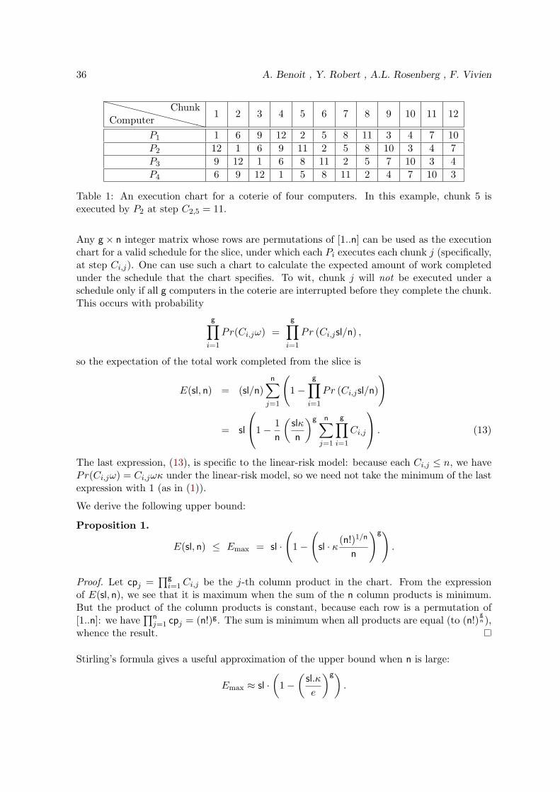
36 A. Benoit , Y. Robert , A.L. Rosenberg , F. Vivien
XXXXXXXXXXXComputerChunk
1 2 3 4 5 6 7 8 9 10 11 12
P1 1 6 9 12 2 5 8 11 3 4 7 10P2 12 1 6 9 11 2 5 8 10 3 4 7P3 9 12 1 6 8 11 2 5 7 10 3 4P4 6 9 12 1 5 8 11 2 4 7 10 3
Table 1: An execution chart for a coterie of four computers. In this example, chunk 5 isexecuted by P2 at step C2,5 = 11.
Any g× n integer matrix whose rows are permutations of [1..n] can be used as the executionchart for a valid schedule for the slice, under which each Pi executes each chunk j (specifically,at step Ci,j). One can use such a chart to calculate the expected amount of work completedunder the schedule that the chart specifies. To wit, chunk j will not be executed under aschedule only if all g computers in the coterie are interrupted before they complete the chunk.This occurs with probability
g∏i=1
Pr(Ci,jω) =g∏i=1
Pr (Ci,jsl/n) ,
so the expectation of the total work completed from the slice is
E(sl, n) = (sl/n)n∑j=1
(1−
g∏i=1
Pr (Ci,jsl/n)
)
= sl
1− 1n
(slκ
n
)g n∑j=1
g∏i=1
Ci,j
. (13)
The last expression, (13), is specific to the linear-risk model: because each Ci,j ≤ n, we havePr(Ci,jω) = Ci,jωκ under the linear-risk model, so we need not take the minimum of the lastexpression with 1 (as in (1)).
We derive the following upper bound:
Proposition 1.
E(sl, n) ≤ Emax = sl ·
(1−
(sl · κ(n!)1/n
n
)g).
Proof. Let cpj =∏gi=1Ci,j be the j-th column product in the chart. From the expression
of E(sl, n), we see that it is maximum when the sum of the n column products is minimum.But the product of the column products is constant, because each row is a permutation of[1..n]: we have
∏nj=1 cpj = (n!)g. The sum is minimum when all products are equal (to (n!)
gn ),
whence the result.
Stirling’s formula gives a useful approximation of the upper bound when n is large:
Emax ≈ sl ·(
1−(
sl.κ
e
)g).

Static Strategies for Worksharing with Unrecoverable Interruptions 37
5.2.2 Group schedules: introduction
Referring back to Table 1, we observe that chunks 1, 2, 3, and 4 are always executed atthe same steps, by different computers; the same is true for chunks 5, 6, 7, 8 as a group, andfor chunks 9, 10, 11, 12 as a group. The twelve chunks of the slice thus partition naturallyinto three groups. By respecifying the schedule of Table 1 as the group(-oriented) schedule
Group 1 Group 2 Group 3chunks 1–4 chunks 5–8 chunks 9–12
1 2 36 5 49 8 712 11 10
Table 2: Execution chart for a group-oriented schedule. Rows represent time steps for the firstcomputer in each group associated with each column; the remaining computers’ schedules areobtained by cyclic downward permutations of the rows.
of Table 2, we significantly simplify the specification. Note that the meanings of rows andcolumns have changed in this re-orientation: compare Tables 1 and 2 as we describe thechanges. In the group(-oriented) execution chart of Table 2, each column corresponds to agroup of chunks; entry (i, j) of the chart specifies the step at which each computer executesits ith chunk within group j. The schedule for computer Pj , where j ∈ {2, 3, 4}, is obtainedby cyclically permuting (downward) the schedule for P1 j − 1 times. The important featurehere is that this orchestration has each computer attempt to execute each chunk exactly once.
We generalize this description. When n is a multiple of g, we can sometimes convert the fullg× n execution chart C, as exemplified by Table 1, to the g× n/g group(-oriented) executionchart C exemplified by Table 2. There are n/g groups, each of size g, and chart-entry Ci,jdenotes the step at which group j of chunks is executed for the ith time. It is tacitly assumedthat chunk-indices within each group are cyclically permuted (downward) at each step, sothat each chunk ends up being processed by each computer. Thus, in order for a chart C tospecify a valid group schedule, its total set of entries must be a permutation of [1..n]. WhenC does specify a valid group schedule, the expected amount of work it completes, under thelinear risk model, is:
E(sl, n) = sl
1− g
n
(sl · κ
n
)g n/g∑j=1
g∏i=1
Ci,j
. (14)
The preceding expression exposes the importance of the constant
K(Θ) =n/g∑j=1
g∏i=1
C(Θ)i,j
as a measure of a group schedule Θ’s performance; to wit,
E(Θ)(sl, n) = sl− K(Θ) · gκ
(slκ
n
)g+1
. (15)

38 A. Benoit , Y. Robert , A.L. Rosenberg , F. Vivien
Thus: A smaller value of K(Θ) corresponds to a larger value of E(Θ)(sl, n).
Group schedules are very natural, because they are symmetric: all computers play the samerole as the work is processed, differing only in the times at which they process different chunks.Intuition suggests that the most productive schedules are symmetric: why should some of theidentical computers be treated differently by “nature” than others? Indeed, the followingupper bound on the expected work production of group schedules—which is the best we havebeen able to prove—does not distinguish symmetric schedules from general ones—but we havenot yet been able to prove that no difference exists.
Proposition 2. For any group schedule Θ,
E(Θ)(sl, n) ≤ Emax = sl− slg+1κg(n!)g/n
ng.
Proof. Let cpj =∏gi=1Gi,j be the j-th column product. As before, E(sl, n) is maximum when
the sum of the ng column products is minimum. The product of these column products is
equal to a constant (n!). The sum is minimum when all products are equal to (n!)gn , hence
the same result as for Proposition 1.
Note that Proposition 2 affords us an easy lower bound, Kmin on the K value of any groupschedule with the parameters g and n:
Kmin =⌈
n
g(n!)g/n
⌉.
5.2.3 Group schedules: specific schedules
Our group schedules strive to maximize expected work completion by having every computerattempt to compute every chunk. Of course, there are many ways to achieve this coverage,and the form of the risk function will make some ways more advantageous than others withrespect to maximizing expected work completion. As an extreme example, in the case p = 2,for every risk function, it is advantageous to have the remote computers process the workthey share “in opposite orders” (Theorem 4). We now specify and compare the performanceof five group schedules whose chunk-scheduling regimens seem to be a good match for theway the linear risk function “predicts” interruptions. We specify each schedule Θ via its groupexecution chart C(Θ)—see Fig. 6—and we represent the performance of each schedule Θ viaits performance constant K(Θ). The beneficent structures of these schedules is evidenced byour ability to present explicit symbolic expressions for their K constants.
Cyclic scheduling (Fig. 6(a)). Under this simplest scheduling regimen, Θcyclic, groupsare executed sequentially, in a round-robin fashion. Specifically, the chunks of group j areexecuted at steps j, j + n/g, j + 2n/g, and so on. We find that
K(Θcyclic) =n/g∑j=1
g−1∏k=0
(j + kn/g) .

Static Strategies for Worksharing with Unrecoverable Interruptions 39
Group 1 Group 2 Group 31 2 34 5 67 8 910 11 12
(a) Cyclic: K = 3104
Group 1 Group 2 Group 31 2 36 5 49 8 712 11 10(b) Reverse: K = 2368
Group 1 Group 2 Group 31 2 34 5 69 8 712 11 10
(c) Mirror: K = 2572
Group 1 Group 2 Group 31 2 36 5 47 8 912 11 10
(d) Snake: K = 2464Group 1 Group 2 Group 3
1 2 38 6 49 7 510 11 12(e) Fat snake: K = 2364
Figure 6: Five group schedules with their associated K values. For this instance, Kmin = 2348.
The weakness of Θcyclic is that chunks in low-index groups have a higher probability of beingcompleted successfully than do chunks in high-index groups—because chunks remain in thesame relative order throughout the computation. The remaining schedules that we consideraim to compensate for this imbalance via different intuitively motivated strategies.
Reverse scheduling (Fig. 6(b)). A schedule Θreverse produced under this regimen executesthe chunks in each group once in the initially-specified order, and then executes them in thereverse order n/g− 1 times. The schedule thereby strives to compensate for the imbalance inchunks’ likelihoods of being completed created by their initial order of processing. (Θreverse isthe schedule specified in Table 2.) Under Θreverse, the chunks in group j are executed at stepj, and thereafter at steps 2n/g − j + 1, 3n/g − j + 1, 4n/g − j + 1, and so on. We find that
K(Θreverse) =n/g∑j=1
j ×g−1∏k=1
((k + 1)n/g − j + 1) .
Mirror scheduling (Fig. 6(c)). The mirror schedule Θmirror, which is defined only when gis even, represents a compromise between the cyclic and reverse scheduling strategies. Θmirror
compensates for the imbalance in likelihood of completion only during the second half of thecomputation. Specifically, Θmirror mimics Θcyclic for the first g/2 phases of processing a group,

40 A. Benoit , Y. Robert , A.L. Rosenberg , F. Vivien
and it mimics Θreverse for the second g/2 phases. We find that
K(Θmirror) =n/g∑j=1
12g−1∏k=0
(j + kn/g) ((p− k)n/g − j + 1) .
Snake-like scheduling (Fig. 6(d)). Our fourth schedule, Θsnake, compensates for the im-balance of the cyclic schedule by mimicking Θcyclic at every odd-numbered step and mimickingΘreverse at every even-numbered step, thereby lending a snake-like structure to the executionchart C(Θsnake). We find that
K(Θsnake) =n/g∑j=1
12g−1∏k=0
(j + 2kn/g) (2(k + 1)n/g − j + 1) .
Fat snake-like scheduling (Fig. 6(e)). Our final, fifth schedule, Θfat−snake, qualitativelyadopts the same strategy as does Θsnake, but it slows down the return phase of the latterschedule. Consider, for illustration, three consecutive rows of C(Θfat−snake). The first row isidentical to its shape in C(Θcyclic). The return phase of Fat snake distributes elements of thetwo remaining rows in the reverse order, two elements at a time. The motivating intuition isthat the slower return would further compensate for the imbalance in Θcyclic. We find that
K(Θfat−snake) =n/g−1∑j=0
13g−1∏k=0
(1 + j + 3kn/g) (3(k + 1)n/g − 2j − 1) (3(k + 1)n/g − 2j) .
We derive the following performance bounds for these five schedules
Proposition 3. The values of K(Θ) for our five scheduling algorithms satisfy the followinglower and upper bounds:
1n
≤ K(Θcyclic)
g! (n/g)g+1 ≤ 1
12g
≤ K(Θreverse)
g! (n/g)g+1 ≤ 12(n + g)
1n
≤ K(Θmirror)
g! (n/g)g+1 ≤ 1
g
n2≤ K(Θsnake)
g! (n/g)g+1 ≤ 1
1(g − 1)n
≤ K(Θfat−snake)
g! (n/g)g+1 ≤ g

Static Strategies for Worksharing with Unrecoverable Interruptions 41
Proof. The calculations are straightforward. For the Cyclic schedule, we have
Kcyclic =
ng∑
j=1
g−1∏k=0
(j + k
n
g
).
We derive the lower bound by replacing index j by 0 in the summation (except in the termk = 0 where we replace j by 1):
Kcyclic ≥n
g
(g−1∏k=1
kn
g
)= (g − 1)!
(n
g
)g
=1ng!(
n
g
)g+1
.
Similarly, we let j = ng in each term of the summation to get the upper bound. We proceed
in a similar way for the other three variants.
We explicit the computations for Fat snake, as they are a bit less obvious. For the lowerbound we have:
Kfat−snake =∑ n
g−1
j=0
∏ g3−1
k=0
(1 + j + 3k n
g
)(3(k + 1)n
g − 2j − 1)(
3(k + 1)ng − 2j
)≥∑ n
g−1
j=0
∏ g3−1
k=0
(1 + 3k n
g
)(3(k + 1)n
g − 2ng + 1
)(3(k + 1)n
g − 2ng + 2
)≥ n
g
∏ g3−1
k=0
(1 + 3k n
g
)((3k + 1)n
g
)((3k + 1)n
g
)≥(
ng
)3∏ g3−1
k=1
(3k n
g
)((3k + 1)n
g
)((3k + 1)n
g
)≥(
ng
)3∏ g3−1
k=1
((3k − 1)n
g
)(3k n
g
)((3k + 1)n
g
)=(
ng
)g(g − 2)!
For the upper bound we derive:
Kfat−snake =∑ n
g−1
j=0
∏ g3−1
k=0
(1 + j + 3k n
g
)(3(k + 1)n
g − 2j − 1)(
3(k + 1)ng − 2j
)≤∑ n
g−1
j=0
∏ g3−1
k=0
(ng + 3k n
g
)(3(k + 1)n
g
)(3(k + 1)n
g
)≤ n
g
∏ g3−1
k=0
((3k + 1)n
g
)((3k + 3)n
g
)((3k + 3)n
g
)≤(
ng
)g+1 (∏ g3−2
k=0 (3k + 2)(3k + 3)(3k + 4))
(g − 2)g2
=(
ng
)g+1(g − 2)!(g − 2)g2 ≤
(ng
)g+1(g)!g
From the size of its bounds on K(Θsnake), Proposition 3 suggests that schedule Θsnake may bethe most efficient of the five group-scheduling algorithms we have considered, especially whenwe checkpoint often, i.e., when n is large. We evaluate this possibility via the experimentsreported at the end of this subsection. While still focusing on mathematical analyses of ourschedules, though, we use Stirling’s formula to derive more evocative bounds on K(Θsnake):Kmin ≤ K(Θsnake) ≤ Kupper, where
Kmin ≈e
g
(n
g
)g+1
and Kupper = g!(
n
g
)g+1
≈ e√
2π√g
(n
g
)g+1
.
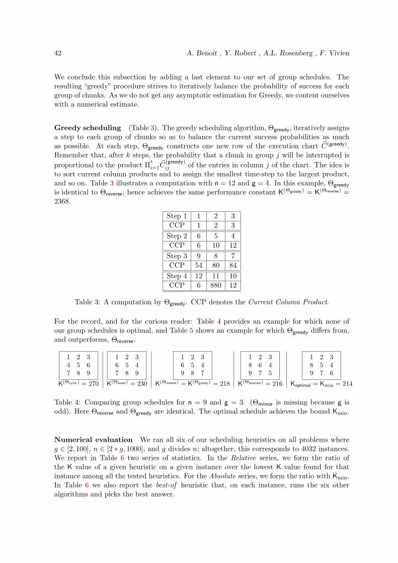
42 A. Benoit , Y. Robert , A.L. Rosenberg , F. Vivien
We conclude this subsection by adding a last element to our set of group schedules. Theresulting “greedy” procedure strives to iteratively balance the probability of success for eachgroup of chunks. As we do not get any asymptotic estimation for Greedy, we content ourselveswith a numerical estimate.
Greedy scheduling (Table 3). The greedy scheduling algorithm, Θgreedy, iteratively assignsa step to each group of chunks so as to balance the current success probabilities as muchas possible. At each step, Θgreedy constructs one new row of the execution chart C(greedy).Remember that, after k steps, the probability that a chunk in group j will be interrupted isproportional to the product Π
k
i=1C(greedy)ij of the entries in column j of the chart. The idea is
to sort current column products and to assign the smallest time-step to the largest product,and so on. Table 3 illustrates a computation with n = 12 and g = 4. In this example, Θgreedy
is identical to Θreverse, hence achieves the same performance constant K(Θgreedy) = K(Θreverse) =2368.
Step 1 1 2 3CCP 1 2 3
Step 2 6 5 4CCP 6 10 12
Step 3 9 8 7CCP 54 80 84
Step 4 12 11 10CCP 6 880 12
Table 3: A computation by Θgreedy. CCP denotes the Current Column Product.
For the record, and for the curious reader: Table 4 provides an example for which none ofour group schedules is optimal, and Table 5 shows an example for which Θgreedy differs from,and outperforms, Θreverse.
1 2 34 5 67 8 9
1 2 36 5 47 8 9
1 2 36 5 49 8 7
1 2 38 6 49 7 5
1 2 38 5 49 7 6
K(Θcyclic) = 270 K(Θsnake) = 230 K(Θreverse) = K(Θgreedy) = 218 K(Θfatsnake) = 216 Koptimal = Kmin = 214
Table 4: Comparing group schedules for n = 9 and g = 3. (Θmirror is missing because g isodd). Here Θreverse and Θgreedy are identical. The optimal schedule achieves the bound Kmin.
Numerical evaluation We ran all six of our scheduling heuristics on all problems whereg ∈ [2, 100], n ∈ [2 ∗ g, 1000], and g divides n; altogether, this corresponds to 4032 instances.We report in Table 6 two series of statistics. In the Relative series, we form the ratio ofthe K value of a given heuristic on a given instance over the lowest K value found for thatinstance among all the tested heuristics. For the Absolute series, we form the ratio with Kmin.In Table 6 we also report the best-of heuristic that, on each instance, runs the six otheralgorithms and picks the best answer.

Static Strategies for Worksharing with Unrecoverable Interruptions 43
1 2 3 4 56 7 8 9 1011 12 13 14 1516 17 18 19 20
1 2 3 4 56 7 8 9 1015 14 13 12 1120 19 18 17 16
1 2 3 4 510 9 8 7 615 14 13 12 1120 19 18 17 16
K(Θcyclic) = 34104 K(Θmirror) = 27284 K(Θreverse) = 24396
1 2 3 4 510 9 8 7 611 12 13 14 1520 19 18 17 16
1 2 3 4 514 12 10 8 615 13 11 9 716 17 18 19 20
1 2 3 4 510 9 8 7 615 14 13 12 1120 19 18 16 17
K(Θsnake) = 25784 K(Θfat−snake) = 24276 K(Θgreedy) = 24390
Table 5: Comparing group schedules for n = 20 and g = 4. Here the most efficient schedulesare ΘFatsnake, Θgreedy, and Θreverse (in this order). The lower bound is Kmin = 23780.
Relative Absolute Success ratemin max avg. stdv. min max avg. stdv.
Cyclic 1.1 3.786 2.143 0.664 1.1 3.786 2.239 0.592 00.00%Reverse 1 1.295 1.055 0.065 1 1.295 1.117 0.061 12.42%Mirror 1 2.468 1.504 0.393 1 2.468 1.575 0.338 12.37%Snake 1 1.199 1.127 0.059 1 1.291 1.193 0.059 12.34%Greedy 1 1.055 1.005 0.015 1 1.224 1.067 0.074 83.01%Worm 1 1.442 1.123 0.115 1 1.530 1.192 0.143 17.07%Best-of 1 1 1 0 1 1.224 1.061 0.069 100.00%
Table 6: Statistics on the K value of all heuristics for 2 ≤ g ≤ 100 and 2g ≤ n ≤ 1000(minimum, maximum, average value and standard deviation over the 4032 instances).
Θgreedy is clearly the best heuristic: it finds the best schedule for 83% of the instances, andits solutions are never more than 6% worse than the best solution found. More importantly,its performance constant is never more than 23% larger than the lower bound Kmin, and, onaverage, it is less than 7% larger than this bound. In fact, only Θfat−snake happens sometimes tofind better solutions than Θgreedy; however, these improvements are marginal, as one can see bycomparing the absolute performance of Θgreedy and best-of. As a result of this experimentation,we retain only Θgreedy as the exemplar of group schedules for the experiments of Section 6.
5.3 Choosing the Optimal Number of Chunks
To this point, we have assumed that the number n of chunks per computer was given tous. In fact, we show now that (happily) one does not have to guess at this value. We beginto flesh out this remark by noting that we can easily obtain an explicit expression for theexpected work completed by any group schedule under the charged-initiation model, fromthat schedule’s analogous expectation under the free-initiation model.

44 A. Benoit , Y. Robert , A.L. Rosenberg , F. Vivien
Theorem 7. (p remote computers: charged-initiation model)Let C be a group schedule defined by the execution chart
Ci,j∣∣i∈{1,...,g},j∈{1,...,n/g} .
If sl(c) ≤ min {sl, X − nε}, then:
E(c,n)(sl(c), C) =sl(c)
sl(c) + nεE(f,n)(sl(c) + nε, C).
Proof. Because of the condition sl(c) ≤ min {sl + nε,X}, Eq. (15) can be used with sl(c) + nεinstead of sl. After rewritting we get:
n
sl(c) + nε
(E(f,n)(sl(c) + nε, C)− sl(c) − nε
)= −K(C)
((sl(c)
n+ ε
)κ
)g
.
Now, we can directly compute E(c,n)(sl(c), C):
E(c,n)(sl(c), C) =sl(c)
n
n∑j=1
(1−
g∏i=1
Pr(c)
(Ci,j
sl(c)
n
))
=sl(c)
n
n∑j=1
(1−
g∏i=1
Ci,j
(sl(c)
n+ ε
)κ
)
= sl(c) − sl(c)
n
((sl(c)
n+ ε
)κ
)g n∑j=1
g∏i=1
Ci,j
= sl(c) − sl(c)
n
((sl(c)
n+ ε
)κ
)g
K(C)
= sl(c) +sl(c)
n
n
sl(c) + nε
(E(f,n)(sl(c) + nε, C)− sl(c) − nε
)=
sl(c)
sl(c) + nεE(f,n)(sl(c) + nε, C).
Now we can determine the value of n, making only the assumption that the expectation of thegroup schedule within the charged-initiation model is a unimodal function of n. (It is quitenatural to assume that this expectation is non-decreasing with n under the free-initiationmodel.) We can, then, use a binary search to seek the optimum value of n. Specifically, foreach tested value m we compare the values of the expectation for m and m+ 1 to determineif the expectation is still increasing in m, in which case m is smaller than the optimum n.The binary search can be safely performed in the interval [1..X/ε].
6 Experiments
We have performed a suite of simulation experiments in order to gain insight into the perfor-mance of the group heuristics on large simulated platforms that are subject to unrecoverable

Static Strategies for Worksharing with Unrecoverable Interruptions 45
interruptions. We report only on the observed behavior of Θgreedy for two reasons, first be-cause of its preeminence in the experiment reported in Table 6, and second, because oursimulations show only small differences among our six heuristics. The source code for all sixgroup heuristics can be found at http://graal.ens-lyon.fr/~abenoit/code/failure.c.
6.1 The Experimental Plan
We use randomly generated platforms made of p computers. In all experiments, we setκ = 1, and we choose the times for interruptions randomly chosen between 0 and 1, followinga uniform distribution. The size of the workload, Wtot, varies between 1 and p. Wtot =1 represents the case in which all computers can potentially do all the work before beinginterrupted; Wtot = p represents the case in which we can do no better than deploy one sliceof size 1 on each computer (which will then compute until it is interrupted).
The key parameters in our experiment are: the number of computers, p; the total amountof work Wtot; the chunk size, cs; and the start-up cost ε. In the experiments, three of theseparameters are fixed while the fourth one varies.
We compare several heuristics:
H1-brute– This brute replication heuristic replicates the entire workload onto all computers.Each computer executes work in the order of receipt, starting from the first chunk, untilit is interrupted.
H2-norep– This no replication heuristic distributes the work in a round-robin fashion, withno replication. Thus, each computer is allocated Wtot/p units of work (rounded by thechunk size).
H3-cyclicrep– This cyclic replication heuristic distributes the work in round-robin fashion,as does H2-norep, but it keeps distributing chunks, starting from chunk 1 again, untileach computer has a total (local) workload of 1. Note that when the number of chunksis a multiple of p, this heuristic is identical to H2-norep, since the chunks assigned to acomputer during the replication phase were already assigned to it previously.
H4-randomrep– This random replication heuristic distributes a total workload of 1 to eachcomputer, but it chooses chunks randomly, to ensure that all chunks deployed on thesame computer are distinct. However, the same chunk can be assigned to several com-puters.
H5-groupgreedy– This group greedy heuristic is the schedule Θgreedy of Section 5.2.2. Sinceour number of chunks n may not be a multiple of g, the last group of computers maynot have a full g chunks to process. In this case, we ignore this last group once itscomputers have been assigned as many time-steps as its number of chunks.
H6-omniscient– This last omniscient heuristic is an idealized static heuristic that knowsexactly when each computer is interrupted. This idealized knowledge obviates replica-tion: each computer is statically allocated precisely as many chunks as it can processbefore its interruption, and only distinct chunks are sent. Of course no actual heuristiccan beat this optimal omniscient heuristic.

46 A. Benoit , Y. Robert , A.L. Rosenberg , F. Vivien
6.2 Experimental Results
Heuristic min max average standard deviationH1-brute 0.017199 1.000000 0.300934 0.316694H2-norep 0.000000 1.000000 0.941108 0.156558H3-cyclicrep 0.333333 1.000000 0.973718 0.070451H4-randomrep 0.166667 1.000000 0.929911 0.106433H5-groupgreedy 0.333333 1.000000 0.980068 0.055115H6-omniscient 1.000000 1.000000 1.000000 0.000000
Table 7: Relative statistics on the overall simulations (2,696,800 instances): the work achievedby one heuristic on one instance is divided by the work achieved by the best heuristic for thatinstance.
In the following, we output the ratio Wdone/Wtot, where Wdone is the amount of work suc-cessfully completed by a heuristic, and Wtot is the total amount of work that had to beprocessed. The experiments have been conducted by averaging the result obtained on 100different random configurations of the system (processor failure times).
(E1) Fixed p, cs and ε
In this first experiment, we analyse the impact of the workload on the heuristics. The totalamount of work Wtot varies between 1 and the number of processors p, which are the twoextreme cases. The chunk size is fixed at 1/n+ ε, where n is the number of chunks per unitof work. We fix the values n = 97, 100, 997 and ε = 0.001, 0.00001. Finally, we experimentwith p = 10 and p = 80 processors.
Figure 7 presents the results with ε = 0.001 for all other combinations of parameters, whileFigure 8 shows the behaviour when ε = 0.00001.
First we can notice that in all plots, as expected, H6-omniscient always return the best result,and H1-brute the worse one. The other heuristics are more comparable with each other. Inall cases, H3-cyclicrep is better than H2-norep, but these two heuristics are equivalent whenthe total number of chunks is a multiple of the number of processors, as can be observed onFigures 7(c), 7(d), 8(c) and 8(d). Notice that the total number of chunks increases with thetotal workload, which explains the particular behaviour of H3-cyclicrep in Figures 7(d) and8(d).
Compared to these last two heuristics, H4-randomrep is generally getting better results thanH2-norep for small workloads. This can be easily explained by the fact that replication allowsto process chunks that fail in the case with no replication. However, when the workloadincreases, then H4 may distribute several times the same chunk while it succeeds on the firstprocessor on which it was assigned. Thus, duplicated work will be completed. Of course,when the cyclic replication is useless, H4 is also better than H3 for small workloads.
Finally, the group greedy heuristic is in most cases the best one (aside from the optimal H6),at least when the workload is not too large. When the workload increases, since the numberof chunks is not necessarily a multiple of the cardinality of groups g, the handling of somechunks may not be optimized. Moreover, for a high workload, a cyclic distribution of thework will achieve a good result since not much redundant work can be done.
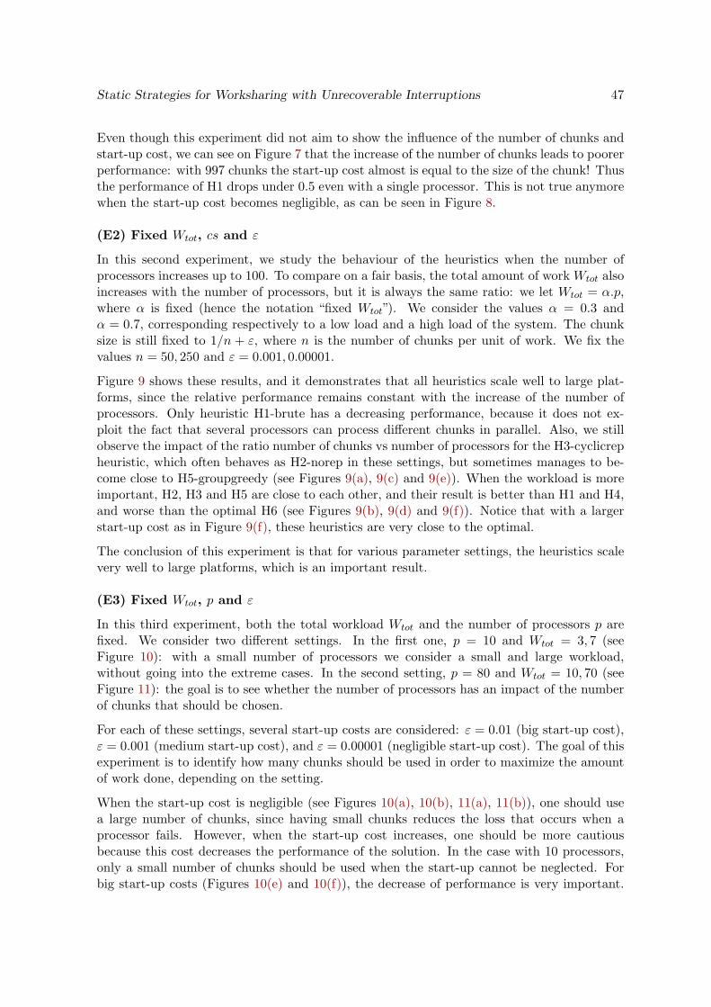
Static Strategies for Worksharing with Unrecoverable Interruptions 47
Even though this experiment did not aim to show the influence of the number of chunks andstart-up cost, we can see on Figure 7 that the increase of the number of chunks leads to poorerperformance: with 997 chunks the start-up cost almost is equal to the size of the chunk! Thusthe performance of H1 drops under 0.5 even with a single processor. This is not true anymorewhen the start-up cost becomes negligible, as can be seen in Figure 8.
(E2) Fixed Wtot, cs and ε
In this second experiment, we study the behaviour of the heuristics when the number ofprocessors increases up to 100. To compare on a fair basis, the total amount of work Wtot alsoincreases with the number of processors, but it is always the same ratio: we let Wtot = α.p,where α is fixed (hence the notation “fixed Wtot”). We consider the values α = 0.3 andα = 0.7, corresponding respectively to a low load and a high load of the system. The chunksize is still fixed to 1/n + ε, where n is the number of chunks per unit of work. We fix thevalues n = 50, 250 and ε = 0.001, 0.00001.
Figure 9 shows these results, and it demonstrates that all heuristics scale well to large plat-forms, since the relative performance remains constant with the increase of the number ofprocessors. Only heuristic H1-brute has a decreasing performance, because it does not ex-ploit the fact that several processors can process different chunks in parallel. Also, we stillobserve the impact of the ratio number of chunks vs number of processors for the H3-cyclicrepheuristic, which often behaves as H2-norep in these settings, but sometimes manages to be-come close to H5-groupgreedy (see Figures 9(a), 9(c) and 9(e)). When the workload is moreimportant, H2, H3 and H5 are close to each other, and their result is better than H1 and H4,and worse than the optimal H6 (see Figures 9(b), 9(d) and 9(f)). Notice that with a largerstart-up cost as in Figure 9(f), these heuristics are very close to the optimal.
The conclusion of this experiment is that for various parameter settings, the heuristics scalevery well to large platforms, which is an important result.
(E3) Fixed Wtot, p and ε
In this third experiment, both the total workload Wtot and the number of processors p arefixed. We consider two different settings. In the first one, p = 10 and Wtot = 3, 7 (seeFigure 10): with a small number of processors we consider a small and large workload,without going into the extreme cases. In the second setting, p = 80 and Wtot = 10, 70 (seeFigure 11): the goal is to see whether the number of processors has an impact of the numberof chunks that should be chosen.
For each of these settings, several start-up costs are considered: ε = 0.01 (big start-up cost),ε = 0.001 (medium start-up cost), and ε = 0.00001 (negligible start-up cost). The goal of thisexperiment is to identify how many chunks should be used in order to maximize the amountof work done, depending on the setting.
When the start-up cost is negligible (see Figures 10(a), 10(b), 11(a), 11(b)), one should usea large number of chunks, since having small chunks reduces the loss that occurs when aprocessor fails. However, when the start-up cost increases, one should be more cautiousbecause this cost decreases the performance of the solution. In the case with 10 processors,only a small number of chunks should be used when the start-up cannot be neglected. Forbig start-up costs (Figures 10(e) and 10(f)), the decrease of performance is very important.

48 A. Benoit , Y. Robert , A.L. Rosenberg , F. Vivien 0
0.2
0.4
0.6
0.8
1
0 2 4 6 8 10
Wd
on
e/W
tot
Total workload Wtot
H1-bruteH2-norep
H3-cyclicrepH4-randomrep
H5-groupgreedyH6-omniscient
0
0.2
0.4
0.6
0.8
1
0 2 4 6 8 10
Wd
on
e/W
tot
Total workload Wtot
(a) 10 processors, 97 chunks.
0
0.2
0.4
0.6
0.8
1
0 10 20 30 40 50 60 70 80W
done/W
tot
Total workload Wtot
(b) 80 processors, 97 chunks.
0
0.2
0.4
0.6
0.8
1
0 2 4 6 8 10
Wdone/W
tot
Total workload Wtot
(c) 10 processors, 100 chunks.
0
0.2
0.4
0.6
0.8
1
0 10 20 30 40 50 60 70 80
Wd
on
e/W
tot
Total workload Wtot
(d) 80 processors, 100 chunks.
0
0.2
0.4
0.6
0.8
1
0 2 4 6 8 10
Wdone/W
tot
Total workload Wtot
(e) 10 processors, 997 chunks.
0
0.2
0.4
0.6
0.8
1
0 10 20 30 40 50 60 70 80
Wd
on
e/W
tot
Total workload Wtot
(f) 80 processors, 997 chunks.
Figure 7: (E1) with ε = 0.001, varying Wtot.

Static Strategies for Worksharing with Unrecoverable Interruptions 49 0
0.2
0.4
0.6
0.8
1
0 2 4 6 8 10
Wd
on
e/W
tot
Total workload Wtot
H1-bruteH2-norep
H3-cyclicrepH4-randomrep
H5-groupgreedyH6-omniscient
0
0.2
0.4
0.6
0.8
1
0 2 4 6 8 10
Wdone/W
tot
Total workload Wtot
(a) 10 processors, 97 chunks.
0
0.2
0.4
0.6
0.8
1
0 10 20 30 40 50 60 70 80W
do
ne
/Wto
t
Total workload Wtot
(b) 80 processors, 97 chunks.
0
0.2
0.4
0.6
0.8
1
0 2 4 6 8 10
Wd
on
e/W
tot
Total workload Wtot
(c) 10 processors, 100 chunks.
0
0.2
0.4
0.6
0.8
1
0 10 20 30 40 50 60 70 80
Wd
on
e/W
tot
Total workload Wtot
(d) 80 processors, 100 chunks.
0
0.2
0.4
0.6
0.8
1
0 2 4 6 8 10
Wd
on
e/W
tot
Total workload Wtot
(e) 10 processors, 997 chunks.
0
0.2
0.4
0.6
0.8
1
0 10 20 30 40 50 60 70 80
Wdone/W
tot
Total workload Wtot
(f) 80 processors, 997 chunks.
Figure 8: (E1) with ε = 0.00001, varying Wtot.

50 A. Benoit , Y. Robert , A.L. Rosenberg , F. Vivien 0
0.2
0.4
0.6
0.8
1
0 2 4 6 8 10
Wd
on
e/W
tot
Total workload Wtot
H1-bruteH2-norep
H3-cyclicrepH4-randomrep
H5-groupgreedyH6-omniscient
0
0.2
0.4
0.6
0.8
1
0 20 40 60 80 100
Wd
on
e/W
tot
Number of processors
(a) α = 0.3, n = 50, ε = 0.00001.
0
0.2
0.4
0.6
0.8
1
0 20 40 60 80 100W
done/W
tot
Number of processors
(b) α = 0.7, n = 50, ε = 0.00001.
0
0.2
0.4
0.6
0.8
1
0 20 40 60 80 100
Wd
on
e/W
tot
Number of processors
(c) α = 0.3, n = 250, ε = 0.00001.
0
0.2
0.4
0.6
0.8
1
0 20 40 60 80 100
Wd
on
e/W
tot
Number of processors
(d) α = 0.7, n = 250, ε = 0.00001.
0
0.2
0.4
0.6
0.8
1
0 20 40 60 80 100
Wd
on
e/W
tot
Number of processors
(e) α = 0.3, n = 50, ε = 0.001.
0
0.2
0.4
0.6
0.8
1
0 20 40 60 80 100
Wd
on
e/W
tot
Number of processors
(f) α = 0.7, n = 250, ε = 0.001.
Figure 9: (E2): varying p.

Static Strategies for Worksharing with Unrecoverable Interruptions 51
It is less obvious in the intermediate case of ε = 0.001 (Figures 10(c) and 10(d)), but evenin this case, the performance decreases when the number of chunks is more important. Ofcourse, care should be taken about the exact number of chunk if using H3-cyclicrep whoseperformance fluctuates, as observed before.
When there are more processors in the system, the influence of the start-up cost is lessimportant; for instance in the case of a big workload, even with ε = 0.01, one can use up to1000 chunks per unit of work with no decrease in the performance (Figure 11(f)).
However, for all settings, if the chunk size becomes significantly smaller than the start-upcost, the performance of all heuristics decreases.
(E4) Fixed Wtot, p, and cs
In this last set of experiments, we study the impact of the start-up cost on the solution.Values of ε are taken between 0 and 1. We consider values of n = 10, 100, 500.
First we run simulations with p = 10 processors (see Figure 12). In this case, as soon as thechunks are small enough (n ≥ 100), the start-up cost has an important effect on the result,and the performance of all heuristics decreases drastically with the increase of ε. Moreover, assoon as the start-up cost is large enough, all heuristics (except H1) find the optimal solution.There is still a difference only in the case Wtot = 1 and n = 100 (Figure 12(c)) and for n = 10(Figures 12(a) and 12(b)). These plots confirm the ranking of the different heuristics: H4-randomrep is better than H2-norep and H3-cyclicrep for small values of ε in Figure 12(a), andthe group heuristic H5-groupgreedy is most of the time better than the three other heuristics.Note that H4-randomrep has a very random behaviour which was not observed before.
Results are quite similar when tackling a platform with p = 50 processors (see Figure 13).Due to the small workload Wtot = 1 on Figures 13(a), 13(c) and 13(e), the whole work canbe replicated onto all processors, using different permutations of chunks, and the differencebetween the different heuristics can be observed. With the increase of the workload (Wtot =10, 30) the start-up cost has less impact on the performance of the heuristics.
6.3 Summarizing the Experiments
The experiments have confirmed the fact that all of our group heuristics implement an effi-cient way to distribute chunks. In many cases, H5-groupgreedy (Θgreedy) provides the optimalsolution. However, we observe that for some values of the parameters, H5-groupgreedy per-forms only slightly better than simpler heuristics such as H3-cyclicrep. For heavily loadedsystems, a simple cyclic distribution of work can even be better than any sophisticated groupheuristic, because we cannot ensure that the number of chunks will always be a multiple of g,and this cardinality may not even be fixed within a large computation: there may be groupswith different values, g or g − 1.
These experiments have also showed the impact of the start-up cost on the solution; inparticular, the simulations allow us to determine how many chunks should be used in orderto maximize the work done, for a given setting. If the start-up cost is negligible, small chunkscan be used, but this strategy becomes disadvantageous with big start-up costs.

52 A. Benoit , Y. Robert , A.L. Rosenberg , F. Vivien
0
0.2
0.4
0.6
0.8
1
0 2 4 6 8 10
Wd
on
e/W
tot
Total workload Wtot
H1-bruteH2-norep
H3-cyclicrepH4-randomrep
H5-groupgreedyH6-omniscient
0
0.2
0.4
0.6
0.8
1
0 200 400 600 800 1000
Wd
on
e/W
tot
Number of chunks
(a) Wtot = 3, ε = 0.00001.
0
0.2
0.4
0.6
0.8
1
0 200 400 600 800 1000W
do
ne
/Wto
t
Number of chunks
(b) Wtot = 7, ε = 0.00001.
0
0.2
0.4
0.6
0.8
1
0 200 400 600 800 1000
Wd
on
e/W
tot
Number of chunks
(c) Wtot = 3, ε = 0.001.
0
0.2
0.4
0.6
0.8
1
0 200 400 600 800 1000
Wd
on
e/W
tot
Number of chunks
(d) Wtot = 7, ε = 0.001.
0
0.2
0.4
0.6
0.8
1
0 200 400 600 800 1000
Wdone/W
tot
Number of chunks
(e) Wtot = 3, ε = 0.01.
0
0.2
0.4
0.6
0.8
1
0 200 400 600 800 1000
Wdone/W
tot
Number of chunks
(f) Wtot = 7, ε = 0.01.
Figure 10: (E3) with 10 processors: varying cs.

Static Strategies for Worksharing with Unrecoverable Interruptions 53 0
0.2
0.4
0.6
0.8
1
0 2 4 6 8 10
Wd
on
e/W
tot
Total workload Wtot
H1-bruteH2-norep
H3-cyclicrepH4-randomrep
H5-groupgreedyH6-omniscient
0
0.2
0.4
0.6
0.8
1
0 200 400 600 800 1000
Wdone/W
tot
Number of chunks
(a) Wtot = 10, ε = 0.00001.
0
0.2
0.4
0.6
0.8
1
0 200 400 600 800 1000W
do
ne
/Wto
t
Number of chunks
(b) Wtot = 70, ε = 0.00001.
0
0.2
0.4
0.6
0.8
1
0 200 400 600 800 1000
Wd
on
e/W
tot
Number of chunks
(c) Wtot = 10, ε = 0.001.
0
0.2
0.4
0.6
0.8
1
0 200 400 600 800 1000
Wd
on
e/W
tot
Number of chunks
(d) Wtot = 70, ε = 0.001.
0
0.2
0.4
0.6
0.8
1
0 200 400 600 800 1000
Wdone/W
tot
Number of chunks
(e) Wtot = 10, ε = 0.01.
0
0.2
0.4
0.6
0.8
1
0 200 400 600 800 1000
Wdone/W
tot
Number of chunks
(f) Wtot = 70, ε = 0.01.
Figure 11: (E3) with 80 processors: varying cs.
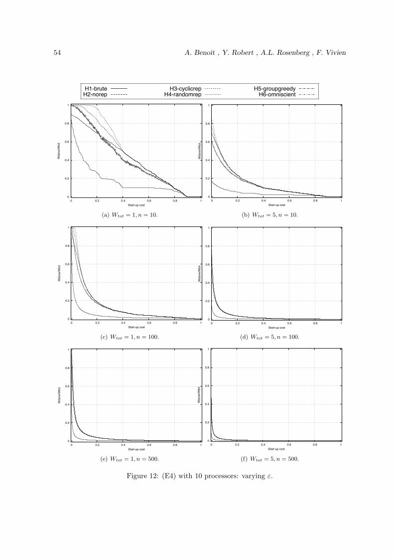
54 A. Benoit , Y. Robert , A.L. Rosenberg , F. Vivien 0
0.2
0.4
0.6
0.8
1
0 2 4 6 8 10
Wd
on
e/W
tot
Total workload Wtot
H1-bruteH2-norep
H3-cyclicrepH4-randomrep
H5-groupgreedyH6-omniscient
0
0.2
0.4
0.6
0.8
1
0 0.2 0.4 0.6 0.8 1
Wdone/W
tot
Start-up cost
(a) Wtot = 1, n = 10.
0
0.2
0.4
0.6
0.8
1
0 0.2 0.4 0.6 0.8 1W
do
ne
/Wto
t
Start-up cost
(b) Wtot = 5, n = 10.
0
0.2
0.4
0.6
0.8
1
0 0.2 0.4 0.6 0.8 1
Wd
on
e/W
tot
Start-up cost
(c) Wtot = 1, n = 100.
0
0.2
0.4
0.6
0.8
1
0 0.2 0.4 0.6 0.8 1
Wdone/W
tot
Start-up cost
(d) Wtot = 5, n = 100.
0
0.2
0.4
0.6
0.8
1
0 0.2 0.4 0.6 0.8 1
Wd
on
e/W
tot
Start-up cost
(e) Wtot = 1, n = 500.
0
0.2
0.4
0.6
0.8
1
0 0.2 0.4 0.6 0.8 1
Wd
on
e/W
tot
Start-up cost
(f) Wtot = 5, n = 500.
Figure 12: (E4) with 10 processors: varying ε.

Static Strategies for Worksharing with Unrecoverable Interruptions 55 0
0.2
0.4
0.6
0.8
1
0 2 4 6 8 10
Wd
on
e/W
tot
Total workload Wtot
H1-bruteH2-norep
H3-cyclicrepH4-randomrep
H5-groupgreedyH6-omniscient
0
0.2
0.4
0.6
0.8
1
0 0.2 0.4 0.6 0.8 1
Wd
on
e/W
tot
Start-up cost
(a) Wtot = 1, n = 10.
0
0.2
0.4
0.6
0.8
1
0 0.2 0.4 0.6 0.8 1W
do
ne
/Wto
t
Start-up cost
(b) Wtot = 10, n = 10.
0
0.2
0.4
0.6
0.8
1
0 0.2 0.4 0.6 0.8 1
Wdone/W
tot
Start-up cost
(c) Wtot = 1, n = 100.
0
0.2
0.4
0.6
0.8
1
0 0.2 0.4 0.6 0.8 1
Wdone/W
tot
Start-up cost
(d) Wtot = 10, n = 100.
0
0.2
0.4
0.6
0.8
1
0 0.2 0.4 0.6 0.8 1
Wdone/W
tot
Start-up cost
(e) Wtot = 1, n = 500.
0
0.2
0.4
0.6
0.8
1
0 0.2 0.4 0.6 0.8 1
Wd
on
e/W
tot
Start-up cost
(f) Wtot = 30, n = 10.
Figure 13: (E4) with 50 processors: varying ε.
56 A. Benoit , Y. Robert , A.L. Rosenberg , F. Vivien
7 Conclusion
We have presented a model for studying the problem of scheduling large divisible workloadson p identical remote computers that are vulnerable (with the same risk function) to unre-coverable interruptions (Section 2). Our goal has been to find schedules for allocating workto the computers and for scheduling the checkpointing of that work, in a manner that maxi-mizes the expected amount of work completed by the remote computers. Most of the resultswe report assume that the risk of a remote computer’s being interrupted increases linearlywith the amount of time that the computer has been available to us; a few results providescheduling guidelines for more general risks.
We have completely solved this scheduling problem for the case of p = 1 remote computer(Section 3). Our solution provides exactly optimal schedules—whose expected work comple-tion is exactly maximum—both for the free-initiation model, wherein checkpointing incurs nooverhead, and the charged-initiation model, wherein checkpointing does incur an overhead.For the case of p = 2 remote computers, we provide schedules whose expected work com-pletion is asymptotically optimal, as the size of the workload grows without bound; we alsoprovide some guidelines for deriving exactly optimal schedules (Section 4). The complexityof the development in Section 4 suggests that the general case of p remote computers will beprohibitively difficult, even with respect to deriving asymptotically optimal schedules. There-fore, we settle in this general case for deriving a number of well-structured heuristics, whosequality can be assessed via explicit expressions for their expected work outputs (Section 5).Simulations suggest that one of our six heuristics—regrettably, the computationally mostcomplicated one—is the clear winner in terms of performance. An extensive suite of simula-tion experiments suggests that all of our heuristics provide schedules with good expected workoutput, and that the “clear winner” in the competition of Section 5 does, indeed, dominatethe others (Section 6).
Much remains to be done regarding this important problem, but three directions stand outas perhaps the major outstanding challenges. One of these is to extend our (asymptotic-)optimality results to a larger class of risk functions, thereby covering the range of situationsthat our work addresses. A second is to extend our study to include heterogeneous assemblagesof remote computers, whose constituent computers differ in speed and other computationalresources. When the assemblages are heterogeneous, but even when they are homogeneous, itwould be significant to allow the assemblage’s computers to be subject to differing probabilitiesof being interrupted.
Acknowledgment. The work of A. Benoit and Y. Robert was supported in part by theANR StochaGrid project. The work of A. Rosenberg was supported in part by US NSF GrantCNS-0842578.
References
[1] M. Adler, Y. Gong, A.L. Rosenberg (2003): Asymptotically optimal worksharing inHNOWs: how long is “sufficiently long?” 36th Ann. Simulation Symp., 39–46.

Static Strategies for Worksharing with Unrecoverable Interruptions 57
[2] M. Adler, Y. Gong, A.L. Rosenberg (2008): On “exploiting” node-heterogeneous clustersoptimally. Theory of Computing Systs. 42, 465–487.
[3] B. Awerbuch, Y. Azar, A. Fiat, F.T. Leighton (1996): Making commitments in the faceof uncertainty: how to pick a winner almost every time. 28th ACM Symp. on Theory ofComputing, 519–530.
[4] M. Banikazemi, V. Moorthy, D.K. Panda (1998): Efficient collective communication onheterogeneous networks of workstations. Intl. Conf. on Parallel Processing, 460–467.
[5] C. Banino, O. Beaumont, L. Carter, J. Ferrante, A. Legrand, Y. Robert (2004): Schedul-ing strategies for master-slave tasking on heterogeneous remote computer grids. IEEETrans. Parallel and Distr. Systs. 15, 319–330.
[6] G.D. Barlas (1998): Collection-aware optimum sequencing of operations and closed-formsolutions for the distribution of a divisible load on arbitrary remote computer trees. IEEETrans. Parallel and Distr. Systs. 9, 429–441.
[7] O. Beaumont, L. Carter, J. Ferrante, A. Legrand, Y. Robert (2002): Bandwidth-centricallocation of independent tasks on heterogeneous platforms. Intl. Parallel and Distr. Pro-cessing Symp.
[8] O. Beaumont, A. Legrand, Y. Robert (2003): The master-slave paradigm with heteroge-neous processorss. IEEE Trans. Parallel and Distr. Systs. 14, 897–908.
[9] O. Beaumont, L. Marchal, Y. Robert (2005): Scheduling divisible loads with returnmessages on heterogeneous master-worker platforms. High-Performance Computing: The12th Intl. Conf. Lecture Notes in Computer Science 3769, Springer-Verlag, Berlin, 498–507.
[10] M.A. Bender and C.A. Phillips (2007): Scheduling DAGs on asynchronous processors.19th ACM Symp. on Parallel Algorithms and Architectures, 35–45.
[11] V. Bharadwaj, D. Ghose, V. Mani (1994): Optimal sequencing and arrangement indistributed single-level tree networks. IEEE Trans. Parallel and Distr. Systs. 5, 968–976.
[12] V. Bharadwaj, D. Ghose, V. Mani (1995): Multi-installment load distribution in treenetworks with delays. IEEE Trans. Aerospace and Electronic Systs. 31, 555–567.
[13] V. Bharadwaj, D. Ghose, V. Mani, T.G. Robertazzi (1996): Scheduling Divisible Loadsin Parallel and Distributed Systems. J. Wiley & Sons, New York.
[14] S.N. Bhatt, F.R.K. Chung, F.T. Leighton, and A.L. Rosenberg (1997): On optimalstrategies for cycle-stealing in networks of workstations. IEEE Trans. Comp. 46, 545–557.
[15] S.-S. Boutammine, D. Millot, C. Parrot (2006): Dynamically scheduling divisible loadfor grid computing. High-Performance Computing and Communications. In LNCS 4208,Springer-Verlag, Berlin, 763–772.
[16] R. Buyya, D. Abramson, J. Giddy (2001): A case for economy Grid architecture forservice oriented Grid computing. 10th Heterogeneous Computing Wkshp.

58 A. Benoit , Y. Robert , A.L. Rosenberg , F. Vivien
[17] Y.C. Cheng and T.G. Robertazzi (1990): Distributed computation for tree networks withcommunication delays. IEEE Trans. Aerospace and Electron. Systs. 26, 511–516.
[18] W. Cirne and K. Marzullo (1999): The Computational Co-Op: gathering clusters into ametacomputer. 13th Intl. Parallel Processing Symp., 160–166.
[19] P.-F. Dutot (2003): Master-slave tasking on heterogeneous processors. 17th Intl. Paralleland Distributed Processing Symp.
[20] I. Foster and C. Kesselman [eds.] (2004): The Grid: Blueprint for a New ComputingInfrastructure (2nd Edition). Morgan-Kaufmann, San Francisco.
[21] I. Foster, C. Kesselman, S. Tuecke (2001): The anatomy of the Grid: enabling scalablevirtual organizations. Intl. J. Supercomputer Applications.
[22] P. Fraigniaud, B. Mans, A.L. Rosenberg (2005): Efficient trigger-broadcasting in hetero-geneous clusters. J. Parallel and Distributed Computing 65 (2005) 628–642.
[23] L. Gao and G. Malewicz (2007): Toward maximizing the quality of results of dependenttasks computed unreliably. Theory of Computing Systs. 41, 731–752.
[24] M. Harchol-Balter and A. Downey (1996): Exploiting process lifetime distributions fordynamic load balancing. SIGMETRICS’96, 13–24.
[25] R. Kesavan, K. Bondalapati, D.K. Panda (1996): Multicast on irregular switch-basednetworks with wormhole routing. 3rd Intl. Symp. on High-Performance Computer Archi-tecture.
[26] D. Kondo, H. Casanova, E. Wing, F. Berman (2002): Models and scheduling mechanismsfor global computing applications. Intl. Parallel and Distr. Processing Symp.
[27] E. Korpela, D. Werthimer, D. Anderson, J. Cobb, M. Lebofsky (2000): SETI@home:massively distributed computing for SETI. In Computing in Science and Engineering(P.F. Dubois, Ed.) IEEE Computer Soc. Press, Los Alamitos, CA.
[28] M. Litzkow, M. Livny, M.W. Mutka (1988): Condor – A hunter of idle workstations. 8thIntl. Conf. on Distr. Computing Systs., 104–111.
[29] G. Malewicz, A.L. Rosenberg, M. Yurkewych (2006): Toward a theory for schedulingdags in Internet-based computing. IEEE Trans. Comput. 55, 757–768.
[30] G.F. Pfister (1995): In Search of Clusters. Prentice-Hall.
[31] A.L. Rosenberg (1999): Guidelines for data-parallel cycle-stealing in networks of work-stations, I: on maximizing expected output. J. Parallel and Distr. Comput. 59, 31–53.
[32] A.L. Rosenberg (2000): Guidelines for data-parallel cycle-stealing in networks of work-stations, II: on maximizing guaranteed output. Intl. J. Foundations of Computer Science11, 183–204.
[33] A.L. Rosenberg (2001): On sharing bag-of-tasks workloads in heterogeneous networksof workstations: greedier is not better. 3rd IEEE Intl. Conf. on Cluster Computing,124–131.

Static Strategies for Worksharing with Unrecoverable Interruptions 59
[34] A.L. Rosenberg (2002): Optimal schedules for cycle-stealing in a network of workstationswith a bag-of-tasks workload. IEEE Trans. Parallel and Distributed Systs. 13, 179–191.
[35] A.L. Rosenberg (2006): Changing challenges for collaborative algorithmics. In Handbookof Nature-Inspired and Innovative Computing: Integrating Classical Models with Emerg-ing Technologies (A. Zomaya, ed.) Springer, New York, pp. 1–44.
[36] S.W. White and D.C. Torney (1993): Use of a workstation cluster for the physical map-ping of chromosomes. SIAM NEWS, March, 1993, 14–17.
[37] J. Wingstrom and H. Casanove (2008): Probabilistic allocation of tasks on desktop grids.Wkshp. on Large-Scale, Volatile Desktop Grids (PCGrid’08).
[38] Y. Yang and H. Casanova (2003): UMR: A multi-round algorithm for scheduling divisibleworkloads. 17th Intl. Parallel and Distributed Processing Symp.