stationary exponential time series: … 00 @ nps-55-83-008 naval postgraduate school monterey,...

AD-A128 347

UNCLASSIFIED

STATIONARY EXPONENTIAL TIME SERIES: FURTHER MODEL DEVELOPMENT AND A RESIDUAL ANALYSIS(U) NAVAL POSTGRADUATE SCHOOL MONTEREY CA P A LEWIS ET AL. APR 83 NPS-55-83-008 F/G 12/1

1/

• END

6 83 DTIC

'••"•' ' ' '

25 1.0 s« t us 112.0

I.I .8

1.25 11.4 ||.6

MICROCOPY RESOLUTION TEST CHART

NATIONAL BURtAU Of STANDARDS 1%3-A

__^_^^^__

CO 00

@

NPS-55-83-008

NAVAL POSTGRADUATE SCHOOL Monterey, California

o o

DTIC SELECTE

MAY 2 0 1983 D STATIONARY EXPONENTIAL TIME SERIES:

FURTHER MODEL DEVELOPMENT AND

A RESIDUAL ANALYSIS

by

P. A. W. Lewis A. J. Lawrance

April 1983

Approved for public release; distribution unlimited

Prepared for: Chief of Naval Research Arlington, VA 22217

83 05 19 199

NAVAL POSTGRADUATE SCHOOL Monterey, California

Rear Admiral J. J. Ekel und Superintendent

David A. Schrady Provost

This work was supported in part by the Office of Naval Research under Grant NR-42-284.

Reproduction of all or part of this report is authorized.

A. J. Lawrance ' University of Birmingham Birmingham, England

P. A. W. Lewis, Professor Department of Operations Research

Reviewed by:

mJL (an R. Washburn, Chairman

Department of Operations Research

Released by:

WiTliam MT Tolles Dean of Research

I

UNCLASSIFIED SECURITY CLASSIFICATION OF THIS PAGE (Whan Data EntaraO

REPORT DOCUMENTATION PAGE REPORT NUMBER

NPS-55-83-008

READ INSTRUCTIONS BEFORE COMPLETING FORM

I. RECIPIENT'S CATALOG NUMMER 2. OOVT ACCEUIOH NO

£0 -^/A?3>'/\ 4. TITLE (and Subllllm)

STATIONARY EXPONENTIAL TIME SERIES: FURTHER MODEL DEVELOPMENT AND A RESIDUAL ANALYSIS

t. TYPE OF REPORT A PERIOD COVEREO

Technical » PERFORMING ORO. REPORT NUMBER

t. CONTRACT OR GRANT NUMBERS 7. AUTHORr»

A. J. Lawrance P. A. W. Lewis

10. PROGRAM ELEMENT. PROJECT. TASK AREA • WORK UNIT NUMBERS

61153N; RRO14-05-01 N0001483WR30026

*. PERFORMING ORGANIZATION NAME AND ADORESS

Naval Postgraduate School Monterey, CA 93940

It. CONTROLLING OFFICE NAME AND ADDRESS

Chief of Naval Research Arlington, VA 22217

IX. REPORT DATE

April 1983 I*. NUMBER OF PAGES

41 U MONITORING AGENCY NAME I AOORESSftf dlllotonl Inm Controlling OKU») IS. SECURITY CLASS, (ol Ulli upon)

UNCLASSIFIED Ha. OECLASSIFICATION' DOWNGRADING

SCHEDULE

I«. DISTRIBUTION STATEMENT (ol (hi. Report)

Approved for public release; distribution unlimited

17. DISTRIBUTION STATEMENT (ol tho mbolrmct onlorod In Block 30. II dllloronl froa. KopoH)

la. SUPPLEMENTARY NOTES

IS. KEY WORDS (Conllnuo on ravaraa oldo II nacaaaaty and idonilty or Mae* numbot)

autoregressive process NEAR(2) process exponential variables non-normal processes residual analysis wind speed data

20. ABSTRACT (Conllnuo an ravaraa old» If nacaaaatr and Idmniitr or Maa* numott)

A second order autoregressive process in exponential variables, NEAR(2), is established: the distributional assumptions involved in this model highlight a very broad four parameter structure which comb.i.es five exponential random variables into a sixth exponential random variable. The dependency structure of the NEAR(2) process beyond and including autocorrelations is explored using some new ideas on residual analysis for non-normal processes with autoregressive correlation structure. Other applications of the exponential structure are considered briefly. These include exponential time series with negative

DO,:2:M7, 1473 EDITION OF I MOV •» IS OBSOLETE

S/N 0107- LF-0U-6601 UNCLASSIFIED

SECURITY CLASSIFICATION OF THIS PAOI (Wnon Data •nlara«-)

- -.f *»

+r •„. r^z-rr- OF>. "*»•

UNCLASSIFIED »•CUMTV CLAMIPIC ATION OP TMI* PAO« (*lMa Dmtm

correlation and exponential time series with mixed autoregressive-moving average structure. An application to the analysis of a set of wind speed data is included.

S/N 0)02-LF-014-«401 UNCLASSIFIED

••CUftlTV CL AMIFICATION OP THIt PAOCr*K«< DM« Bnl.r.rf)

-r *- . •* "*s - cap*>i,p 21

""••

)'

Stationary Exponential Time Series: Further model development

and a residual analysis

by

A. J. Lawrance Department of Statistics University of Birmingham Birmingham, England

P. A. W. Lewis Department of Operations Naval Postgraduate School Monterey, California, U.S.A.

ABSTRACT

A second order autoregressive process in exponential variables, NEAR(2),

is established: the distributional assumptions involved in this model high-

light a very broad four parameter structure which combines five exponential

random variables into a sixth exponential random variable. The dependency

structure of the NEAR(2) process beyond and including autocorrelations is

explored using some new ideas on residual analysis for non-normal processes

with autoregressive correlation structure. Other applications of the expo-

nential structure are considered briefly. These include exponential time

series with negative correlation and exponential time series with mixed

autoregressive-moving average structure. An application to the analysis of

a set of wind speed data is included. _^-

Aooesnion For

MTIS GR44I DTIC TAB Unannoui'.j • *

I Just in.•'.;:: ! •

it- a a

By JlllStrJbllUr;;/

IvallflfcU'ty Codes 'Avail and/or

Dl»t

± Special

L. January 1983

- -r *- *. • -* esarw^j S V- - r»'

I «

1. Introduction

There are several aspects of many observed univariate time series which

are not satisfactorily accounted for in standard time series analysis: they

include non-Gaussian marginal distributions, dependence beyond second-order

moments (autocorrelations) and directionality in the time series. Quite

often a Gaussian distribution will be inappropriate because the variable

being modelled has a positive and highly skewed distribution, i.e., the

service times in a queue or daily flows in a river. Many particular such

distributions can be envisaged and time series models have been constructed

for them. Examples are Gamma distributions (Gaver and Lewis, 1980; Lewis,

1981; McKenzie, 1982; Lawrance, 1982) and mixed exponential distributions

(Gaver and Lewis, 1980; Lawrance, 1980a; Lawrance and Lewis, 1982)

However the simplest, most widely used and most tractable analytically

of these distribution models is the exponential distribution. Like Gaussian

random variables, exponentially distributed random variables enjoy many

special properties; also they can be mildly transformed quite easily into

distributions which are more skewed,or less skewed, than the exponential. The

Weibull distribution is an example, being just a power transformation of an

exponentially distributed random variable. Thus the approach here, following

earlier work (Gaver and Lewis, 1980; Lawrance and Lewis, 1980, 1981) is to

regard the exponential variables as canonical and to develop their use in

time series modelling. It should also be noted that time series of uniformly

distributed random variables are obtained by exponential transformations of

the exponential time series; this has many possibilities and the process

of uniformly distributed random variables will be considered elsewhere.

The work cited above has concentrated for the most part on first-order,

non-Gaussian autoregressive models, both of the standard type (constant

coefficient additive linear combinations) and a random coefficient type

1

• -*• *• - •* p. f3rt.— t ÜBKMC

introduced by the authors. The extension of the models to higher order

autoregression is clearly necessary to attain flexibility in modelling cor-

relation and dependency structure of the processes, but these extensions are

in no way as immediate as in the standard linear Gaussian case. A simple

mixing device can be used (Jacobs and Lewis, 1983) but the range of correla-

tions attained is much narrower than the range attained in the standard

linear, second-order autoregressive structure. A broader extension, called

the EAR(2) model, was obtained in the exponential case by Lawrance and lewis

(1980), but its innovation variable has a zero component and this will often

be hard to justify.

A major part of the present work consists of obtaining a very broad and

rich extension of the NEAR(l) model (Lawrance and Lewis, 1981) to a second-

order autoregressive process; this NEAR(2) model was first proposed in

Lawrance (1980b) and later reviewed in Raftery (1981), although necessary

analysis of its innovation structure was not given. The innovation random

variable for the NEAR(2) process is proved here to exist without unnatural

boundaries on its (four) parameter region and does not have a zero component.

Taken out of the context of second-order autoregressive exponential time

series this result gives a very broad structure for combination of exponential

random variables. In fact it gives a way to combine three (possibly dependent)

exponential random variables with an independent pair of (possibly dependent)

exponential random variables to give another exponential random variable. The

result has a number of uses beyond the second-order time series model giving,

for instance, a first-order model which is broader than the NEAR(l) model, and

several second-order mixed autoregressive-moving average models. Schemes for

obtaining negative correlation can also be accommodated. These models, as in

the first-order case, include aspects of dependence beyond autocorrelation and

also directionality in the time series.

*^r^^;jj(P«m»-- v- - ca^^t BZ

The richness of the four-parameter NEAR(2) model and the fact that an

infinite number of cases of the model with identical correlation structure

are available forces consideration of higher-order aspects of dependence.

The analysis of the higher order aspects of the exponential time series is

at a fairly early stage and is as follows. First it will be shown that the

autocorrelations PU), ft = 0, + 1, +2,... for the NEAR(2) process satisfy

the Yule-Walker equations with constants a, and a~ which are functions

of the four parameters of the model. This follows immediately from the fact

that X„ is a random-coefficient, linear additive combination of X , , n n-1

X - anc' tne innovation r.v. E . Secondly, it can be shown (Lewis and

Lawrance, 1983a) that the residuals X - a,X , - a~X - > which are the

usual residuals for second-order constant coefficient, linear additive

autoregressive processes are uncorrelated.

Thus although the standard analysis of time series stops with uncorrelated

residuals, i.e. a flat spectrum for the residuals, such residuals can also be

used to good effect to investigate higher order aspects of dependence in the

NEAR(2) model. In fact, if the autoregression is not of the standard type

(constant coefficient, linear additive) the (uncorrelated) residuals will

have non-random scatters and higher order dependence properties. In partic-

ular, the squared residuals will have non-zero autocorrelations and the

cross-correlations of residuals and squared residuals except in the zero-

lag case will be non-zero; both sets of correlations are effectively zero

when a standard second-order autoregressive model is appropriate.

An extension of this residual analysis is suggested by the fact that

autocorrelations are time reversible, while the process itself is not time

reversible, i.e. is directional. Thus one constructs reversed residuals

X - anX ., - a0X ,0 which are to be used to assess directionality. Analysis n I n+i c n+c

r*nr**50fcgp*^* ***** ,<•

B^ ——

of both types of residuals can be fruitful; because of space limitations we

present here only an investigation of cross-correlations of residuals and

squared-residuals. This particular case of the possible residual analyses

is illustrated by some theoretical calculations, some simulations and a brief

application to a transformed series of wind speed data. The complete residual

analysis including directional aspects and their investigation using the

additional tool of reversed residuals will be given elsewhere.

r~^.r'rvi-^i »•- "Vr cs*..~-

2. Exponential Time Series Models

Our aim in this section is to give in outline the ideas leading to the

time series model of main concern in this paper, and called NEAR(2), follow-

ing the earlier terminology NEAR(l). The NEAR(2) model has four-parameters,

and incorporates and broadens the earlier two-parameter EAR(2) model (Lawrance

and Lewis, 1930). The NEAR(2) model will be exponential in marginal distri-

bution, have second-order autoregressive Markov dependence, and have auto-

correlations satisfying second-order difference equations of the familiar

Yule-Walker type. In addition it will have dependence beyond autocorrelation,

and will have adjustable directionality. It is not linear in the standard

sense, having random-coefficient, linear additive autoregressive structure,

but neither is it non-linear in the standard sense of incorporating powers or

products of lagged variables.

Writing {Xn} for the time series variables, and {E } for an i.i.d.

exponential innovation sequence of unit mean, the two-parameter NEAR(l) model,

as previously defined, is given by

(2.1)

with b = (l-a)ß and p = (l-ß)/{l - (l-a)ß} . The parameter region is in

general 0<a, M 1, a= j/ 1 , The case ß = 1, 0 < a < 1 is rather

special, and has been called the TEAR(l) model, and when a = 1, 0 < $ < 1 ,

the earlier EAR(l) model is recovered. Except for this EAR(l) case, the

NEAR(l) model does not allow zero innovations (Gaver and Lewis, 1980) and so

is more statistically acceptable. The zero innovation implies that

X = eX i and thus e can be determined exactly from runs down in the n n-1

sample path of the process.

In general the i.i.d. innovation in the NEAR(l) process are formed as

the probabilistic mixture of two exponentials, and are thus easily simulated.

F The NEAR(2) model is a direct generalization of (2.1) and takes the form

Xn =

*lx„-l W'P- al

h\-2 W-P- a2

0 w.p. 1-a

+ E (2.2)

1 " a2

with parameter region 0 < B,, ß2 £ 1, a, > 0, a„ >_ 0, a, + a- < 1 ; (E 1 is

an appropriately chosen innovation sequence. Many special cases can arise

when the above restrictions include some of the equalities and, for the pur-

poses of a general development, it is best to regard the inequalities as

strict. Given that {Xn} is required to have an exponential marginal distri-

bution, the main question concerns whether there is a valid probability

distribution for E . The Theorem proved in Section 2.3 will show that

this is the case, and that the distribution, when the inequalities on

Oj + 0^ and ß,, p^ in the parameter region are strict, takes tre form

E = 1 n

w.p. 1-p,

b2En w-p- p2 '

3 n w.p. p.

;3 '

(2.3)

a probabilistic mixture of three exponentials. To establish this result a

fairly detailed analysis of a derived moment generating function is required.

This is necessary since a direct moment generating function solution of (2.2)

for E does not establish that E„ has a proper distribution; all that is n n

shown is that the solution is a possibly improper mixture of three exponentials.

* -r *•• - •* T»-»iy:*' v- - -«»:>•*•

T — •

3. Validity of the NEAR(2) Model

In this section we prove the following

THEOREM. Let {E } be an i.i.d. sequence of unit mean exponential random

variables. Then if the four parameters a-,, a2, B-., P2 satisfy

a, > 0, a2 > 0, a, + a„ < 1, 0 < ß,, 2 < 1, the relationship

Xn = <

ßlXn-l w-p* al *

ß2*n-2 w,p' a2 *

0 W.p. 1-a, - a-

+ En , n = 0, + 1, + 2,..., (3*.l)

where

fcn w.p

»2En w.p

»3En w.p

l-p2 - p3 ,

J2 '

J3 »

(3.2)

defines a stationary sequence of (marginally) exponentially distributed

random variables with mean one. Here

P2 * Ka1ß1 + a2ß2)b2 - {a} + Ogjßjßgl/C (t>2 ' b3^1 " b2^} '

p3 = {{a] + a2)ß]B2 - («1ß1 + o^ß^b^/{(b2 - b3)(l - b3)} ,

where

and

S = (1 - a1)ß1 + (1 - cx2)ß2 ,

(3.3)

(3.4)

and

0 < b3 = 1 js - (s2 - *r)1/2j < b2 = 1 |s + (s2 - 4r)| < 1 , (3.5)

(3.6)

r = (1 - a-| - a2)ß-jß2 (3.7)

- -.«•>•• . •* «._.rr^ *i<fg»,+ii* ? Y - cat-.- t mpr

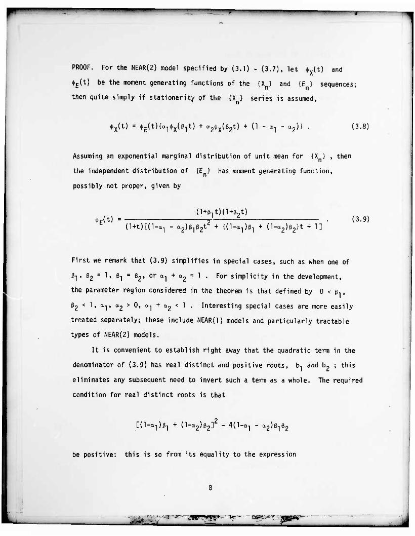
PROOF. For the NEAR(2) model specified by (3.1) - (3.7), let $x(t) and

<(>E(t) be the moment generating functions of the {X } and {E } sequences;

then quite simply if stationarity of the {X } series is assumed, n

*XU) = •E(t){a1*x(ß1t) + a2$x(ß2t) + (1 - a1 - a2)} . (3.8)

Assuming an exponential marginal distribution of unit mean for {X } , then

the independent distribution of {E } has moment generating function,

possibly not proper, given by

•c(t) - J L- . (3.9) (l+t)[(l-a1 - a2)ß1ß2t

c + {(l-a1)ß1 + (l-a2)ß2}t + 1]

First we remark that (3.9) simplifies in special cases, such as when one of

^» &2 = 1' ei = e2' or al + a2 = ^ " For slmPlicity in the development,

the parameter region considered in the theorem is that defined by 0 < ß,,

ß2 < 1, ot-j, a2 > 0, a-j + a2 < 1 . Interesting special cases are more easily

treated separately; these include NEAR(l) models and particularly tractable

types of NEAR(2) models.

It is convenient to establish right away that the quadratic term in the

denominator of (3.9) has real distinct and positive roots, b, and b2 ; this

eliminates any subsequent need to invert such a term as a whole. The required

condition for real distinct roots is that

C(l-a1)ß1 + (l-ct2)ß2]2 - 40-aj - a2)ß1ß2

be positive: this is so from its equality to the expression

f»-'- vr - CSP^T

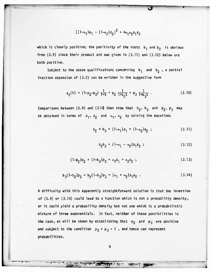
C(l-a1)ß1 - (l-a2)ß2] + 4a1a2ß1ß2

which is clearly positive; the positivity of the roots b, and bo is obvious

from (3.9) since their product and sum given in (3.11) and (3.12) below are

both positive.

Subject to the above qualifications concerning b, and b2 , a partial

fraction expansion of (3.2) can be written in the suggestive form

•E(t) - (1-P2-P3) T?t + P2 üb^t + P3 T^t • (3J0)

Comparisons between (3.9) and (3.1C) then show that b2, b3 and p2, p3 may

be obtained in terms of ß,, ß2 and »1, a2 by solving the equations

b2 + b3 = (1-c^)^ + (l-o2)ß2 ; (3.11)

b2b3 = (1-c^ - «2)^2 ' (3>12)

(l-b2)p2 + (l-b3)p3 = a1ß1 + a2ß2 ; (3.13)

b3(l-b2)p2 + b2(l-b3)p3 = (o1 + 02)3^2 • (3-14)

A difficulty with this apparently straightforward solution is that the inversion

of (3.9) or (3.10) could lead to a function which is not a probability density,

or it could yield a probability density but not one which is a probabilistic

mixture of three exponentials. In fact, neither of these possibilities is

the case, as will be shown by establishing that p2 and p3 are positive

and subject to the condition p2 + p3 < 1 , and hence can represent

probabilities.

9

It

• •• —

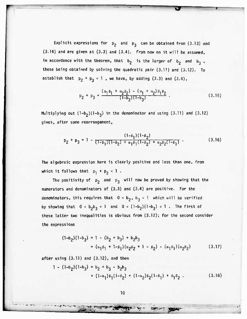
Explicit expressions for p2 and p3 can be obtained from (3.13) and

(3.14) and are given at (3.3) and (3.4). From now on it will be assumed,

in accordance with the theorem, that b2 is the larger of b? and b? ,

these being obtained by solving the quadratic pair (3.11) and (3.12). Jo

establish that p2 + p3 < 1 , we have, by adding (3.3) and (3.4),

P2 + P3 =

(a, e, + a,ß9) - (a, + a,) 1 1 2 2 1 ' u2'plp2 d-b2)(l-b3)

(3.15)

Multiplying out (l-b2)(l-b3) in the denominator and using (3.11) and (3.12)

gives, after some rearrangement,

(l-ß1)d-62) P2 + P3 = ' ~ (l-ß1)(l-ß2) + a^d-ßg) + a2&2(]-^) ' (3.16)

The algebraic expression here is clearly positive and less than one, from

which it follows that p, + p2 < 1 .

The positivity of p2 and p3 will now be proved by showirg that the

numerators and denominators of (3.3) and (3.4) are positive. For the

denominators, this requires that 0 < b2, b3 < 1 which will be verified

by showing that 0 < b2b3 < 1 and 0 < (l-b2)(l-b3) < 1 . The first of

these latter two inequalities is obvious from (3.12); for the second consider

the expressions

(l-b2)(l-b3) = 1 - (b2 + b3) + b2b3

= (a]ß1 + l-ßj)(a2ß2 + 1 - ß2) - (ajßjKagß^

after using (3.11) and (3.12), and then

1 - (l-b2)(l-b3) = b2 + b3 - b2b3

= (l-a^O-ßg) + (l-ogjßgd-ß^ + ßjßg •

(3.17)

(3.18)

10

r****^*^* <£ • ca^t^t ,>

p '• " ' •--

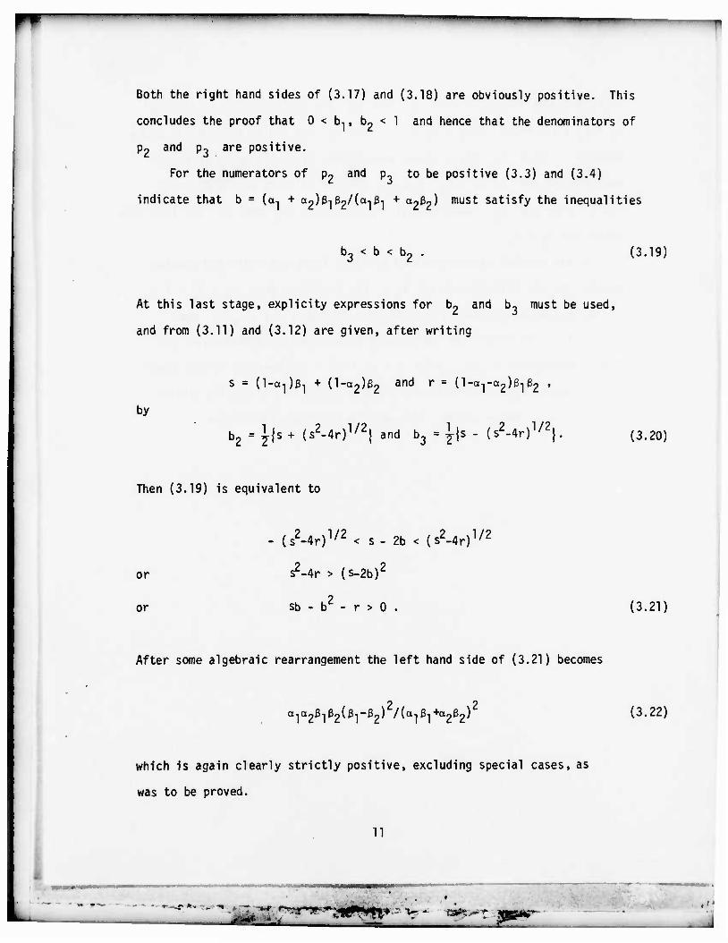
Both the right hand sides of (3.17) and (3.18) are obviously positive. This

concludes the proof that 0 < b,, b, < 1 and hence that the denominators of

P2 and p3 are positive.

For the numerators of p2 and p- to be positive (3.3) and (3.4)

indicate that b • (a, + a2)ßi32/(a,ßi + a2e2^ must satisfy tne inequalities

b, < b < b2 (3.19)

At this last stage, explicity expressions for b2 and b3 must be used,

and from (3.11) and (3.12) are given, after writing

by

s = (1-ot^)ß-j + (l-a2)ß2 and r = (l-a-j-ag)^^ '

b2 = ^{s + (s2-4r)1/2( and b3 = ^s - (s2-4r)1/2>. (3.20)

Then (3.19) is equivalent to

- (s2-4r)1/2 < s - 2b < (s2-4r)1/2

or

or

s2-4r > (s-2b)2

sb - b - r > 0 (3.21)

After some algebraic rearrangement the left hand side of (3.21) becomes

2 2 ala2ßlMßl~ß2^ /(ai^i+a2e2^ (3.22)

which is again clearly strictly positive, excluding special cases, as

was to be proved.

11

—T

r "WH*** v- - •«*?>*•? ,'•

This concludes the proof that p2 and p3 are both positive subject to

p2 + p3 < 1 ; hence l-p2 ~ P3 » P? » an(* P3 can a^ De regarded as prob-

abilities. Thus E has a proper probability distribution which can be

generated as the (l-p2 - P3» P?» P3) mixture of three exponentials of

means 1, b2 and b3 respectively; further, both b2 and b3 are less than

unity and b2 t b3 .

In the special cases mentioned earlier, there are valid and simpler

results for the distribution of E . For instance, when ß, = ß2 = 1 ,

E has a simple exponential distribution of mean (1-a, - o2) . When

ß, = ß2 f 1 the innovation has a mixed exponential distribution of the

NEAR(l) form given in (2.1) with a = a, + a2 . Delineation of all these

special cases is needed for successful simulation of the NEAR(2) process

for the full parameter range. This will be considered elsewhere.

12

•p- -^> *» -. -w •> "VB - ta^^t «P**"' .'

4. Other Uses of the NEAR(2) Exponential Construction

The NEAR(2) process was established by showing that (3.2) was a valid

innovation distribution for the relation (3.1). The distributional assump-

tions implied by this result can also be taken out of the time series context in

which they were derived and viewed generally as a way to combine a pair of

(possibly dependent) unit exponential variables (L,, L2) with an independent

triple of (possibly dependent) unit exponential variables (M,, M2, M3) so

as to yield a further unit exponential variable. Specifically, with

(a-,, a2, &-\, ß2) and (°2' b3» P*' P3) as previously related by (3.3) - (3.7),

the Theorem has established that

ß2L2

w.p.

w.p.

w.p.

al

a2

1-a

+ •

M, w.p.

b2M2 w.p.

b3M3 w.p.

1-Pi

(4.1)

has a unit exponential distribution.

First of all, the idea of "switching" will be illustrated; in the NEAR(2)

context, this suggests taking (M1, M2, M3) as Un_-|> Xn_2, Xn_3) and

(L-j, L2) as (En, En) . Then (4.1) gives the time series model

X_ =

Vi w.p. l-p2- P3 *lEn w.p. al

b2Xn-2 w.p. p2 + ' *2En w.p. a2

b3Xn-3 w.p. P3 0 w.p. 1—1

(4.2)

This is a third-order autoregression, actually a case of the EAR(3) model

cited in Lawrance and Lewis (1979); note, however, that this third-order

autoregressive exponential process allows zero innovations. Another, better

13

1^ - rrr 'id

^

behaved higher-order exponential model -in fact a p-th order model- is

obtained by the following application of the result (4.1) in its original

form (3.1). Let the indices l,2,...,p be partitioned into two non-empty

sets I, and I2 of size t, and t2 respectively. Then in the model

rß'X , 1 n-1 w.p. 1

al • • • • • • • • • • • • • • • • • •

6PVP w.p. ap

0 w.p. T-aj pj

• + En , n - 0, + 1, + 2,..., (4.3)

let $\ = p., f€I-j ß! = ß?, t€l„; I a'. = a1 and £ a\ = ao • Then l€l, i€l2 ' l

if a^ + a2 < 1 , 0 <: ßj, 32 < 1 the distribution of E is given by the

Theorem. Thus we have a pth-order exponential autoregressive process with

four-parameters. However, while this may seem satisfying it is not clear

that four parameters would be sufficient to characterize the sample path

behaviour of an exponential process with very high order dependence.

Another use of (4.1) is to allow L, and 1_2 to both be X , , and

so obtain a four parameter first-order model of the form

•IVI w.p. al

ß2Xn-l w.p. a2

0 w.p. '-I' • a2

w.p. l-p~ - p- ,

¥n w-p- '2 '

b3En w.p. p3 .

(4.4)

Four parameters seems excessive for a first-order autoregressive process but

simulations show a wide range of behaviour in sample paths with different

choices of parameters. Equation (4.4) in turn suggests a first-order model

allowing negative dependence. This is obtained by letting the variable in

14

amr**r «s*w .''

(4.4) which is multiplied by ß9 be the antithetic transformation of X , ,

"Vl that is - log(l-e ) . A two parameter version of the model could be

obtained, for example, taking a, = a- , ß, = ß„ •

A third type of use of the construction is to give mixed autoregressive

moving average models; for this, (L^, Lp) is Un_-|> xn_?)

as previously,

but (M,, M2» M3) are chosen to be (E E^+1, E^) for a second-order moving

average cumpoent, or as (E En+i«

En+2^ ^or a tn"ird~order moving average

component.

Out of the time series context, the construction suggests ways to obtain

multivariate exponential distributions, rather as in Lawrance and Lewis

(1983b).

Further possibilities are numerous, but it is not the intention here to

exhaustively list them, or to derive the details of those cited at this time.

Analysis in the following sections will deal with the basic NEAR(2) model.

15

i

5. Autocorrelation Structure of the NEAR(2) process

In this section we show that the autocorrelations pU) = corr(xn»xn_J»

I = 0, + 1, + 2,... of the NEAR(2) process satisfy Yule-Walker type dif-

ference equations; thus the second moment dependency aspects of the process

are indistinguishable from those of a standard autoregressive model, AR(2).

To show this it is convenient to write the equation (3.1) as an additive

autoregressive combination of X ,, X - and E . Thus we have a random

coefficient, linear additive autoregressive process

where

K * MnXn 1 + Mn*„ 0 + LnE„ n in n-1 Z n r\-c n n

t 1 w. P. 1-P2 - P3 '

b2 w. P. P2 »

b3 w. P- P3 ,

(1,0) w.p. al '

(0,1) w.p. <*2 '

(0,0) w.p. l-a-. - a«

n = 0, + 1, + 2,...,

n = 0, + 1, + 2,...,

0, + 1, + 2,,

(5.1)

(5.2)

(5.3)

and the i.i.d. sequences {Ln} and {K , K } are mutually independent and

independent of the independent exponential sequence {E } . The En's are

assumed to have mean and variance 1 , as do the X 's by construction. • i

Now E(Kn) = a1 and E(Kn) = a2 , so that E(Ln) • l-«^ - a262 '

Then multiplying Xn in (5.1) by Xn_^ we have, for I > 1 ,

E(Vn-£> = W^I-lW + a2e2E(Xn-2Xn-P + E(Ln>E(En>E<Xn-^ = alßlE(Xn-lW + a2ß2E(Xn-2Xn-£) + ] ' Vl " a2ß2 •

so that

E<XnXn-*> " 1 = Vl{E(Xn-lXn-£> " 1} + a2ß2{E(Xn-2Xn-£) " 1}

16

£••- V- e$ß&*t

r

—........ — —

and P(-£) = alP(-(£-l)) + a2p(-0e-2))

where a] = a^ and a2 = a^ . Using P{-1) = P(l), I > l , we have

finally

oil) • a]P(l-l) + a2p(£-2) , I > 1 , (5.4)

which are the Yule-Walker equations for the AR(2) process. The conditions

for a solution to exist (Box and Jenkins, 1970, p.58), a, + a? < 1 ,

a2 > a2 > - 1 are clearly satisfied when the conditions on

<*j» «2' ßl' h 9iven in the Theorem of Section 3 hold. We then have

PO) = a.,/(l-a2) and P(2) = a^O) + a2 . (5.5)

Note, however, the restriction to positive correlations since a1 and a~

are positive. The possible region of (p(l),p(2)) values is bounded below by

p(2) = p (1) and otherwise bounded by p(l) > 0 and p(2) <_ 1 . Broadening

of the model to negative dependency may be achieved using antithetic ideas,

or the bivariate scheme given in Gaver and Lewis (1980), but is not pursued

here.

Note too that the parameters in (5.4) enter only as products a-, = a-iP-.

and a2 • a232 • Thus for small enough a, and a2 , values of ß, and ß2

greater than one could be allowed, and (5.4) would still have a stable

solution. However the sequence E in the defining equation (3.2) may not

exist; it is not known if ß, <_1 and ß2 <_ 1 is a necessary condition for

this existence.

Solutions to (5.4) are given in detail in Box and Jenkins (1970,

pp. 58-60).

17

v-r r-~-> -»y. i»

Am

Specifying allowable values of p(l) and p(2), as may be done by an

initial second order analysis of data, leaves two parameters to be specified

in the model, say a, and a~ which could produce very different sample

path behaviour in the time series. It is important to notice that this

specification of p(l) and p(2) further constrains the range of possible

a, and dp values. Recalling that p(l) and p(2) fix a-i = a-,?,-, and

a~ = apSo' as we^ as tnat »i + ou <_ 1 , 1t Is easily shown that we must

have

a, _< a, and a~ <_ a~ (5.6)

which implies that a, + a» < a, + a» < 1 . Thus a, and a2 are forced

to lie in a triangular subregion of the triangular (a,,«^) region which is

bounded below by a~ , bounded on the left by a, , and bounded above by

the 1ine a, + a2 = 1 .

18

r

—

6. An analysis of wind velocity data

6.1. Discussion of the data

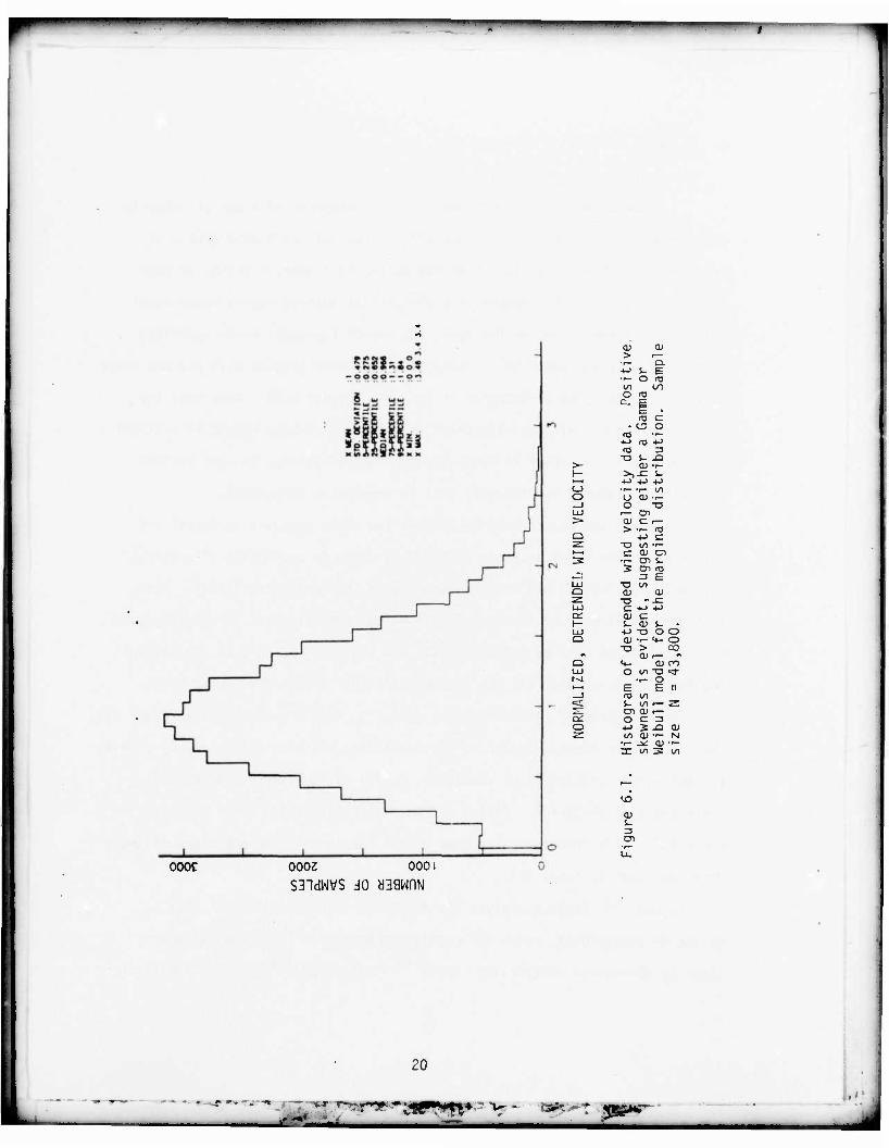
Lewis and Hugus (1983) have given an analysis of a set of 3-hourly

wind velocity readings taken by ship PAPA in the Gulf of Alaska over a 15

year period. After suitable detrending to remove 1 year, 6 month, 12 hour

and 6 hour cyclic trend components a first-order autoregressive Gamma model

(Lewis, 1981) was fitted to the data, the use of the model being suggested

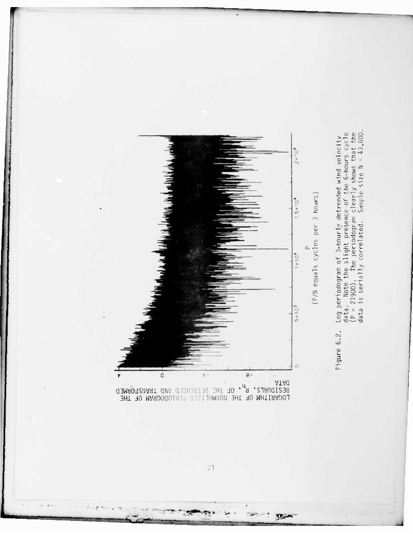
by the shape of the (marginal) histogram of the data (Figure 6.1) and the shape

of the normalized log periodogram of the data (Figure 6.2). Note that the

sample size is N = 43,800; also there is a residual 6-hour effect (P = 21900)

because this cycle varies in intensity over the 15 years. In what follows

this will be ignored and the data will be treated as stationary.

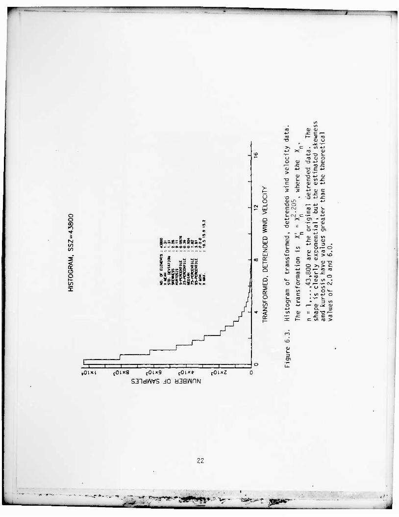
It is not the object here to discuss the above analysis in detail but

to discuss a different analysis of the data using an assumption of a Weibull

marginal distribution and a transformation to exponential variables. This

is suggested firstly by the fact that a Weibull distribution is commonly used

for this type of data by meteorologists and secondly by the fact that Weibull

and Gamma distributions fit the data equally well (Lewis and Hugus, 1983). i p 7Cf\

The histogram of the transformed data, X = X " , is shown in Figure 6,3,

where the power transformation to exponentiality has been determined by fitting

the empirical coefficient of variation, 0.479, to the theoretical Weibull

coefficient of variation, C(X) • {r(2/c + l)/[r(l/c + l)]2} - 1 to give

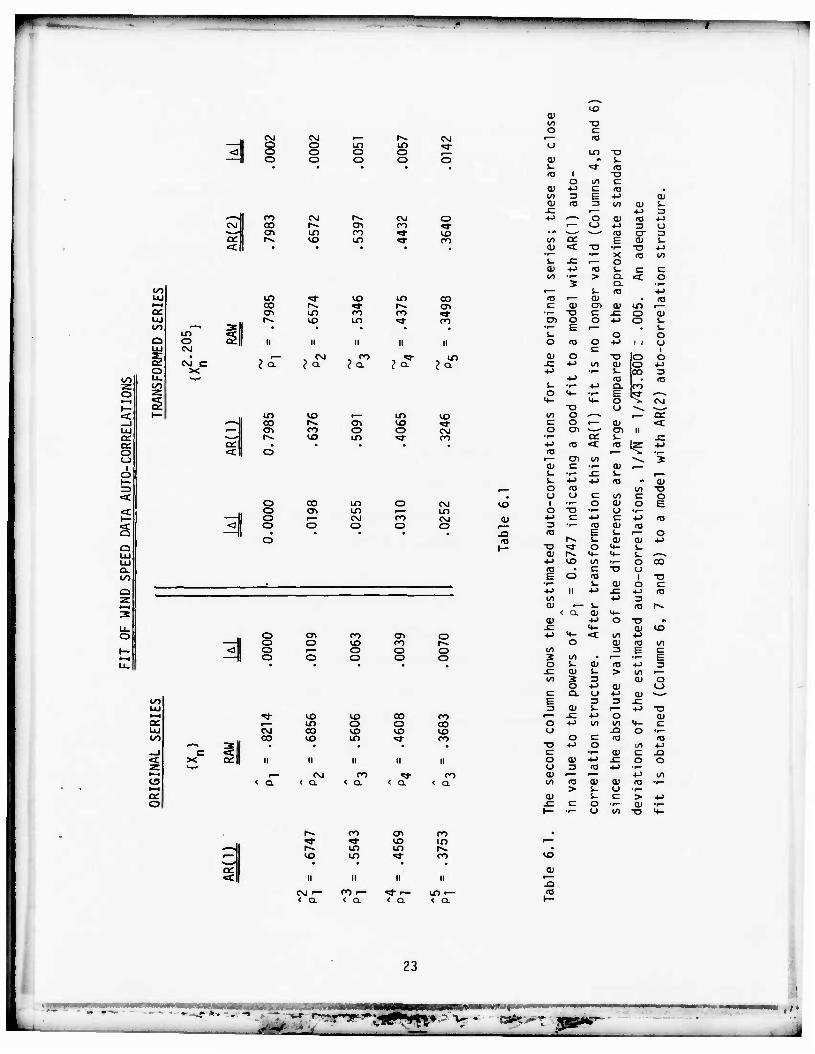
c = 2.205. This transformation does affect the correlation structure of the

data, as shown in Table 6.1.

Column 2 in Table 6.1 gives the estimated auto correlations, PU) ,

of the detrended data; rough 95% confidence bands for these estimates are

given by adding and subtracting 2/(N)1/2 = 2/(43,800)1/2 ~ .01 . The first

19

r

QJ QJ > i—

•1— a. 4~> V- E • f— O ru

CO LO o <0 c.

• QJ ••- (— >i-C S- »—i -l-> 4-> -t-> <_> • r— ••— to o o QJ •,- _l o •o LU 1— Cn > QJ C r— > •i- «3 o +J c •z. "O CO •!— 1—t c QJ C7> 3 •r— CD i_

2 CTi rr; .—; 3 E LU -a l/> O OJ QJ Z -a • -C LU c +J +J Q; 0) c H s_ QJ S_ • LU +-> -o O O O QJ --- 4- O

T3 > CO •* QJ r- - Q 4- QJ ro LU O in "O <t l-J •i- O »—t E E M _J ro LO •a; S_ 1/1 • 7** > cn QJ i— cc O C 13 o -i-> 3JD Q) •z. l/> QJ -I- N

•r— _*: QJ 1- a: 1/13 vi

QJ

oooc 0003 000l

20

g-y^jy^H1 ? V - a*->^: 35s**-

r

a> QJ O >»•— -C o +J <j -l-> CO •- >, » O (J •»-> n c T3 *j-

i— on -£= OJ S. •<-> II > 3

O i/i z: x> -tr 3 C l O GJ •i- to -c M 5 i/i -f—

GJ i/i x> -c >i , a» +-> •— QJ

l/l •a S- i— '- c 4- re CL 3 <D o QJ E c S- i— ro _c

QJ U u uo

ro x> c E QJ ro •

i- >-> 1/1 S_ X3 QJ <— QJ CTl QJ a. s- s_ O *J

3 D.T3 »a i/i O o >— GJ JC +-> •r- QJ

a. i— i x: S- i. u ro en QJ V. >• •i— CL O o 4- i— (J

O i/> QJ 1/1 -c ^ , E UHr- rO (O -C f—

=3 S- +J <0 cr CD • T-

GJ o ai *—. s- X) +-> O QJ o o O 1/1

~^ •r- z ai a. S- i— i/i

•—• QJ Q. •

CNJ —

US II /o en •»-> •!->

O ro Q. ro _l X) ^-X)

QJ S- 3 en

f 0 • - B-

u viva aiMOdsmrai QNVo • in 2H.L JO ' y 'sivnaisjy

3Hi JO wvb9oaoiM3d Q3ZiiVNaON 3Hi JO WHIIUVDOI

; i

* '-- - SP"s J

3 ii IM in

af

I 5 2 ££ ££ hSflBflOISffl^ - 'VdEtinQTiSi

r x

u o _) LiJ > o z $ o Lul Q z UJ a:

»01" i fOtxg c0tx9 cOlxfr

S31dWVS JO a39WnN t0i*Z

-a

*-> X

u o o

Ol •»-) >

c oi •r- .c 3 2

o tu m

•o o c cxi dj • S-CSl c

+-> X Ol

-O il

- - c -a x oi E i- in o •»-

i/i Ol Ol

t— 2 13 0) u

• (/> +-> 03 01

*-> "O l- <o o o

•o « 0)

-U £ -u Ol -r-

"O -4-> Ol C i/> -C O) Ol *->

oi -c < c/> 01 a: •i— .c

CJl *

!- fO 0 —

•*->

01 c .c ai +-> c

o QJ o. S_ X <V Ol

o >, O i— CO s-

n oi •3- •—

• o

• I/)

cr,

CO

Ol

o> 3 •

i— O H3 . > «3

Ol T3 > C ro A3 .C

o •r- CM in o <«- +-> o s. 3 to

_*r CD

<o >

• • - -r *•» . -* , • ,r^r*y^jiPro»-- v C*it. M09* ,'•

3 § CM r— r» CM O en in ^- O o o o o o o

, Jl co CM r*. CM o CM oo I-» en CO «* »M*l en in CO *a- VO BCU r^ VO in **• CO 111 • • • •

00 z o

ce o o

«a:

a. to

oo LÜ »—« Of LU 00

o Uu OO

2

oo O CM

CM C X

1

oo *J- vo If) CO co r» *T r-~ CTi CTl in CO CO «* r^ «3 if) «* CO

• • ' • • ii II II II II

, •> ^ , •*> . «r , oo a. <* Q- ?a Jo. {°-

or

on 10 1— OO <o 00 r~ CT> so «* a» CO O o CM r^ VO OO **• CO

«f o oo OO o CM o <T> OO ^ OO o r— CM CO CM o o o o o

vo

-Q 03

^1 o en CO CT> o o o VO CO r^ o r— o o o o o o o o

•—1 »a- vo vo oo CO or r— oo o o co UJ CM 00 vo VO VO 00 00 VO oo *3" CO

r--> 3l • • • —I c <fl <£ X a= II n n II II Z ^^ »—* ^— CM CO ^r CO o < a < a < a. < a < Q. 1—1

QT O

VO a> 10 •o O c ^— (O u

LD T3 QJ •> i. S- «* <o UJ I •o

O l/l c ai +J c m . CO 3 E 4-> CU cu 03 3 to cu I. sz r— 4-> 3 4J -—• o CU 03 4->

r— c_> +J 3 u • • ^—' 1—* <0 CT 3 VO OT E CU U a; <£ TJ •^ -D 4->

•r— •^ X 03 CO i- x: i— o Cu +-> <o 1. C C CO 'r— > Q. <r o

s a. r— s- TJ •u <o 1— QJ • 03 c ai CD CU oo

•p— -o C x: O CU O) o o 4-> O k •^ E 1— V. s- o o o 03 o

c +-> i i o

1 cu o t3 o o -C +-> to CU o +J +J •1— s- 00 3

•»-> la • 03 s_ •f- +-> o. co o 4- •r~ E *r ^~^ n-

-o <4- O

u S. CM

« o .—N P— or c o r— cu «a: o O) ^—' en n •^ OL S. x: 4J ta <c «13 "5 4-> fO •fW

r— en U1 ^^ 2 QJ c •»— CU ^ S- •^ sz s- r^ S_ +-> +-> (C * CU o 03 00 •o o (J c to c o

1 •f- o cu o E o T3 •r- o •^

+-> C +J c -•-> 03 3 •r— IT3 cu 03 03 E s- i— o

l~~ s- a> CU •M •a «d- o <4- s. cu r^ H- 4- i. ^-^

•u VO to •r- o 00 <o • tz "O u E o (0 1 •o

•r" s- cu o c +J II +-> -C +J 03 vo 4-> 3 cu s- 03 rs.

c a ai <«- CD +J O T3 •1

-SZ <4- CU VO •M <+- < to +->

o CU 03 CO CO 3 E c s to " r— E o i~ a> 03 4-> 3

-C cu (. > to f—

to s 3 CU o o 4-> CU O

c Q. O +-> CU ^- e 3 3 x: 3 01 S- ^— +J •o ^— .c 4-> o cu O •<-> to CO <«- c u XI o

o c 03 03 -o +-> o to 4-y c •r-

CU c •a o ai 4-> SZ o o o 3 <T5 +-> •r— ai r-~ r— •P 10 </> ns CD cu 03 •r>

> S_ o •t—

ai S- e > +J -e c o •r— » oo oo r^

r— VO oo «*• CO

or «i II n n II

CM >— CO •— * r- OO r < a < Ct < a < a.

VO

cu

«3

23

• mmm T£! ,r^ry^5^!H>

•B»^^—

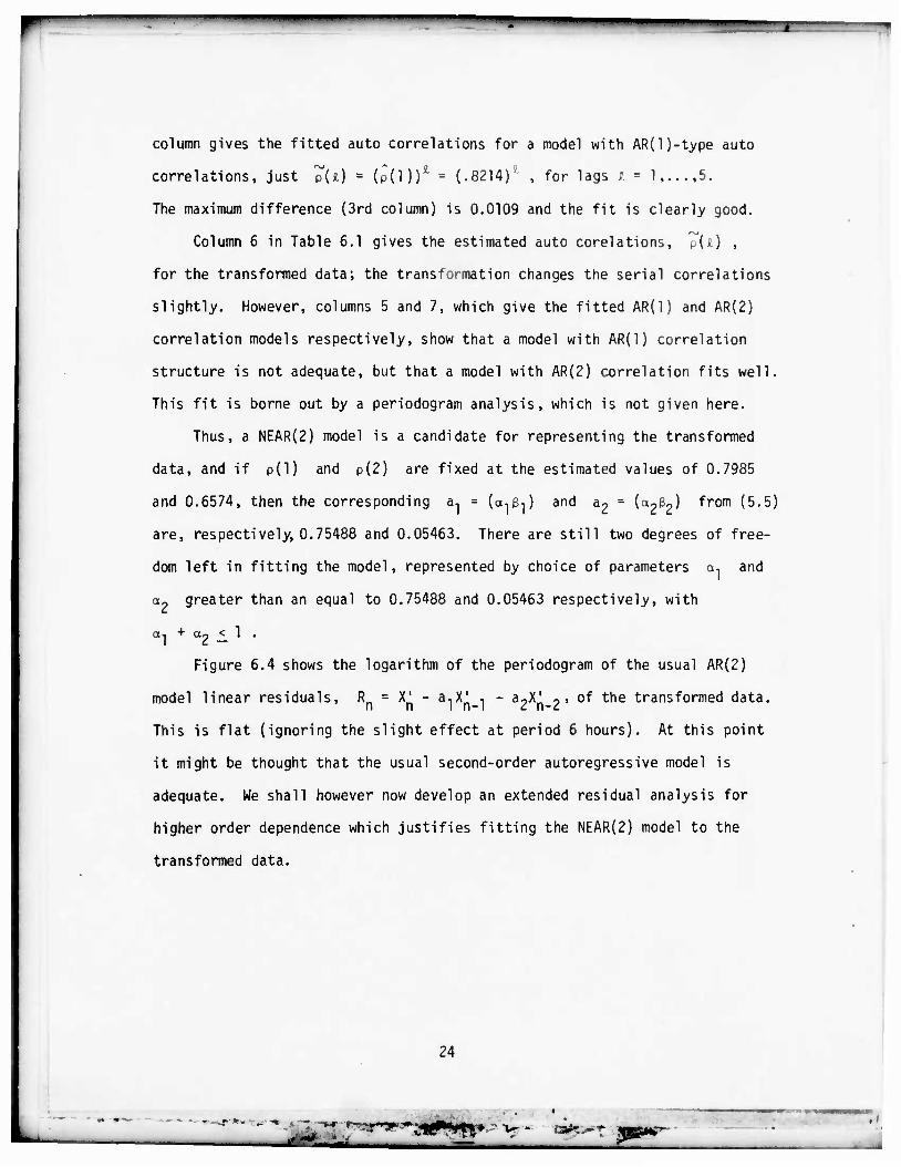
column gives the fitted auto correlations for a model with AR(l)-type auto

correlations, just p(ij • (p(l))e = (.8214)' , for lags i = 1 5.

The maximum difference (3rd column) is 0.0109 and the fit is clearly good.

Column 6 in Table 6.1 gives the estimated auto corelations, p(l) ,

for the transformed data; the transformation changes the serial correlations

slightly. However, columns 5 and 7, which give the fitted AR(1) and AR(2)

correlation models respectively, show that a model with AR(1) correlation

structure is not adequate, but that a model with AR(2) correlation fits well.

This fit is borne out by a periodogram analysis, which is not given here.

Thus, a NEAR(2) model is a candidate for representing the transformed

data, and if p(l) and p(2) are fixed at the estimated values of 0.7985

and 0.6574, then the corresponding a, = (a-jg,) and a2 = (a^ßo) from (5.5)

are, respectively, 0.75488 and 0.05463. There are still two degrees of free-

dom left in fitting the model, represented by choice of parameters a, and

a2 greater than an equal to 0.75488 and 0.05463 respectively, with

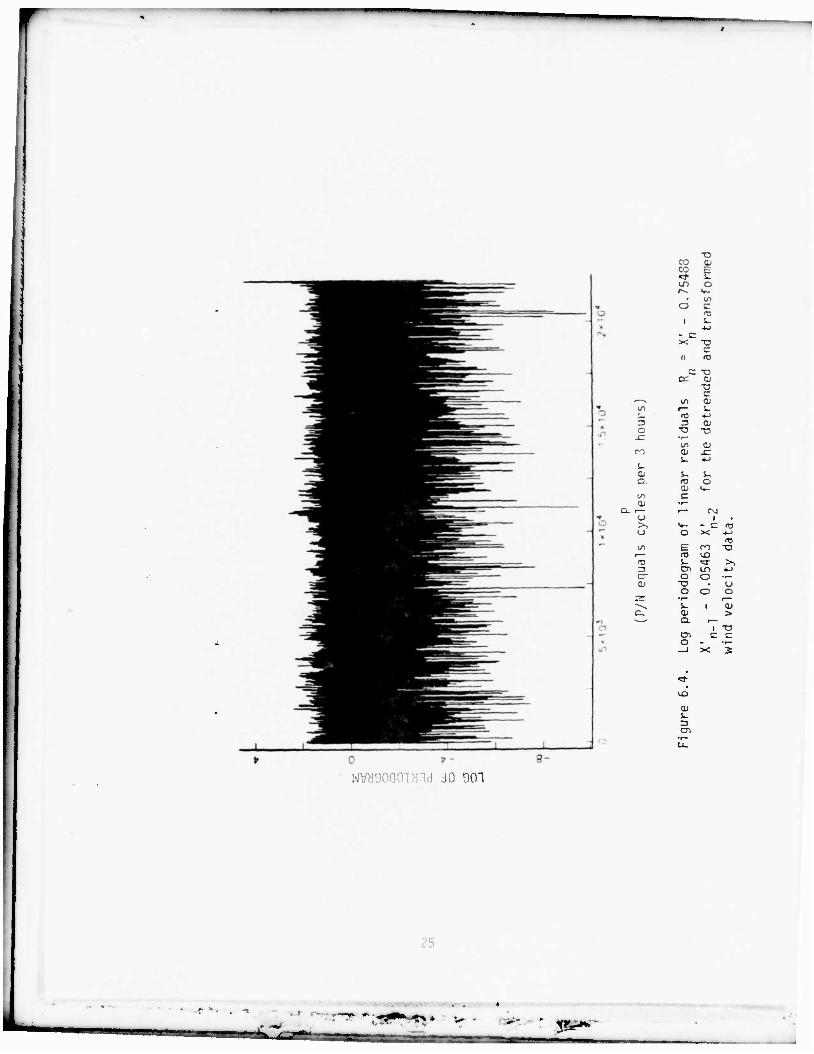
Figure 6.4 shows the logarithm of the periodogram of the usual AR(2)

model linear residuals, R = X' - a,X' , - a^X'o> of the transformed data.

This is flat (ignoring the slight effect at period 6 hours). At this point

it might be thought that the usual second-order autoregressive model is

adequate. We shall however now develop an extended residual analysis for

higher order dependence which justifies fitting the NEAR(2) model to the

transformed data.

24

- "u~ - cs*:^»*- ,'

r

•o co OJ CO h «* i. Ln o r^ It-

- c X •o

c II T3

C 13 cr CJ

C -—* en ai 1/1 r— s_

ro +-> ZJ =5 a> o -a •D .c •f—

oo ai CO GV .c

S- •t-j s_ > i<- - c <o o o X

</> £ CO T3 1— itJ <£> <t> s- <3" >l 3 en IT) 4-> cr o a •t»

o -a I) o o o

2E •j— r— **>, s- i 0) a. ai > *— Q.

i T3 en c c o - • f—

_i X 3

i.

en

wvyynnniHid JO OOI

25

p«r _j

7. A Residual Analysis for the NEAR(2) Model

7.1. General results

It has already been remarked that the autocorrelations p(n) are

insufficient to describe the dependency structure of NEAR(2) models. A

natural next step might be to examine higher joint moments and consider their

associated spectra (see e.g., Priestley, 1982). The functions so obtained, e.g.

the bispectrum, are often found to be difficult to calculate and hard to

interpret. Rather than follow this course, it is proposed to adapt some

ideas from a residual analysis for autoregressive models which has recently

been suggested by the authors (Lewis and Lawrance, 1983). The thrust of

this analysis is that the standard process of fitting and validating a linear

autoregressive model is carried out beyond the customary final stage at which

uncorrelated residuals are obtained (as in the previous section). The usual

presumption is that the residuals are not only uncorrelated but also inde-

pendent. This need not be the case,as will be exemplified for the wind ve-

locity data. Moreover, dependent but uncorrelated residuals are obtained

(Lewis and Lawrance, 1983) even for the NEAR(2) process. Thus the residuals

should be subjected to further analysis in respect of their remaining de-

pendency. Any found is then evidence that a standard linear, constant co-

efficient second-order autoregressive model is deficient. With normally

distributed time series data this might suggest that non-linear modelling

should be explored. With data marginally distributed in some other identi-

fiable manner, then the exploration of a particular type of model with

specified marginal distribution and autocorrelation function is suggested.

This latter course is envisaged here.

26

— - ^*^, ., ^?>ir 9mu^_ . >'.

Higher order dependency properties of the uncorrelated residuals are

obtained for the proposed model and compared with their data counterparts;

this stage can be informative from both exploratory and estimation consid-

erations, and can be thought of as part of the model-refinement process

common to much statistical methodology.

It might be thought that the specific class of NEAR(2) models could be

incorporated in a residual analysis in the standard manner. However, a

moments reflection indicates that even after estimating parameters of (2.2),

it will not be possible, because of the mixture involved, to write down an

expression or recursion for the residual innovations, name)y E . However,

the corresponding autoregressive (or linearized) residual is available and

given, as in the previous section, by

Rn = Xn " alXn-l " a2Xn-2 '

We now show that these are uncorrelated for the NEAR(2) process.

7.2. The residual theorem.

The autocovariances of the residuals (7.1) are

Cov(Rn, Rn+,) - Cov(Xn, Rn+£) - a1Cov(Xn.r R^) - a2Cov(Xn_2, R^)

= Cov(V W " alCov(V Wl* " a2Cov<V W21 '

(7.1)

(7.2)

since the {X } process and consequently the {Rn> process is stationary.

The covariances on the right hand side are all of the same type and given by

Cov(Xn, RnH) - Cov{Xn, (Xn+£ - a^^ - a2Xn+^_2)}

27

(7.3)

(Var(X)}(pU) - alPU-l) - a2pU-2)), % = 1,2,...

•-V;- ca*>^r xmsiv .

By the Yule-Walker equations (5.4) the expression in brackets is zero, and

hence also

Corr(Rn, Rnn) = 0 , *=+!,+ 2,... (7.4)

as was to be proved. That these residuals are uncorrelated is an immediate

consequence of the autocorrelations following Yule-Walker equations; this

emphasizes that this type of residuals will be uncorrelated for any model

whose autocorrelations satisfy Yule-Walker equations.

The analysis of the uncorrelated residuals R ,n = 3,4,... should begin

with scatter plots of the low lag adjacent values; any patterns or concen-

trations will be evidence of dependency in the residuals. Many possibilities

present themselves but only one is pursued in the following Section 8, and

then applied in Section 9 to a continued analysis of the wind velocity data.

28

r 8. Cross-correlation analysis of {R } and {R }

n n

After the satisfactory fit to data of an ordinary linear model, the

residual, Rn, should not only be uncorrelated but also independent; the

latter is customarily investigated by seeking a flat spectrum, while for

the independence, a flat spectrum of the squared residuals can be sought.

As a method for probing model validity, the examination of squared residuals

has been employed by McLeod and Li (1983), following Oranger and Andersen

(1978); these authors suggested bilinear modelling for dependent but un-

correlated residuals of ARMA models. It is suggested here that autocorrela-

tions of squared residuals and cross correlations of residuals of squared

residuals be used in the analysis of higher order dependence of the detrended

transformed wind speed data and its modelling by the NEAR(2) process. The

residuals for this data have already been shown to have a flat spectrum

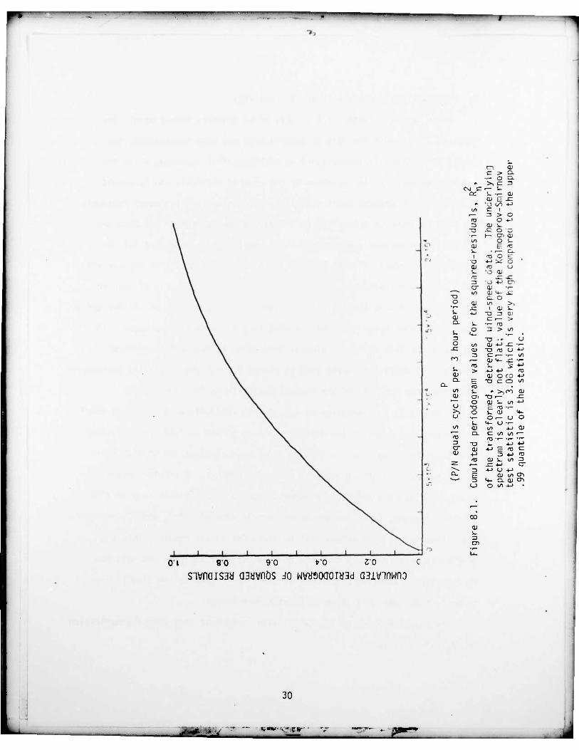
(Figure 6.4) while the curved plot in Figure 8.1 for the cumulative periodogram

shows that the spectrum of the squared residuals is far from flat.

Theoretical investigation of the squared residuals of the NEAR(2) model

is pursued here. Whilst the autocorrelations of the squared residuals have

just been mentioned, for the NEAR(2) model this involves computation of

36 terms, mostly distinct types of 4^ order moments. A simpler suggestion

which involves only third-order moments, and is thus the next step up after 2

autocorrelations, is to use the cross correlations of the Rn and Rn sequences;

apart from lag 0, zero values will be found for linear models. This sug-

gestion is more tractable than the squared residual analysis and will now

be described. Sampling properties of third-order moments are also likely

to be less extreme than those of fourth-order moments.

The starting point of the calculation is to note that from the definition

of Rn at (7.1) that

29

.'•

1

c-> a> c > Q-

•r- o Q- •• >1 C 3 CSJ c ^— LB

cc ai E -C

p •a i/l -t-> l/l c i (— 3 > o tJ O 4-> 3 Ol S-

T3 JC O 3 • »— t— cr. a> l/l o •_ a> E <c

i <T3 o E "O •<-> ^ o a> «3 u s^ 'O 0) 03 -c x: 3 O •u c cr a> •«—

1 • uo CD >*- -t: "o c^ o o Ol in >, ,f~ -C i OJ s- i- -*-J -a 3 ai QJ c f— ^» Q. S^ ID

o ^ > l/l U- tt- .,— « 3 x> . r u O i/i ai *-> _C •^ -C O) T3 <TD O +-•

3 c •— 'i— l/l OO r— a> «•- x: •»—

T3 j£ •!->

t- > 4-> •t-> Cj

<D ai O CO *J

CL £ "O c o </> </l * >,ro "O ^= *— O a> i- l/l *•>

u •o fO 1- >^ o S_ a> u- u o r— O o

s_ 4- <J 1- </> aj l/l +J 01 ^~ a. C l/l l/l <— 03 f0 •T- <l— •1—

3 "a 4-> 4-> O" E ro c QJ +J 3 -!-> m

ra a> S- 00 3 Z -C -l-> cr ^— 3 +-> U +-> Q- E 0) i/i en *— 3 H- ex a> o>

O O l/l •!-> •

CO

OH 80 90 fr'O 3 0 C

sivnaiS3H Q3cjvnös JO wvysoaoiynd Q3ivinwnD

30

— ^—Jlfl

' '•

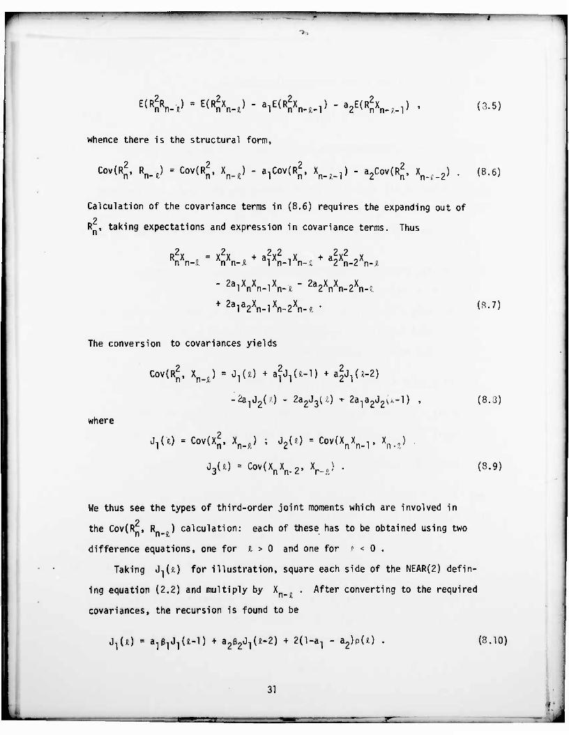
1 E<RnRn-*> - E<RnV*> " alE<RnVM> " a2E(RnXn-?-l' (3.5)

whence there is the structural form,

Cov(R2, Rn_e) - Cov(R2, Xn_2) - alCov(Rn2, X^) - a2Cov(R

2, Xn_;_2) . (8.6)

Calculation of the covariance terms in (8.6) requires the expanding out of 2

R , taking expectations and expression in covariance terms. Thus

RnXn-e = XnXn-A + alVlXn-c + a2Xn-2Xn-*

" 2alXnXn-lV)c ' 2a2XnXn-2Xn-?

+ 2ala2Xn-lXn-2Xn-?, • (a.7)

The conversion to covariances yields

where

Cov(R2, Xn_A) = JjU) + afj1(n-l) + &l^(l-Z)

-2a1J2(>.) - 2a2J3t:) • 2a1a2J2v--'l) ,

^(0 - Cov(X^, Xn_9) ; J2(Jl) = Cov(XnXn_r Xn.J

J3(0 • cov(xnxn.2, xr_£) .

(8.3)

(3.9)

We thus see the types of third-order joint moments which are involved in 2

the Cov(RS Rn .) calculation: each of these has to be obtained using two

difference equations, one for z > 0 and one for t < 0 .

Taking J,U) for illustration, square each side of the NEAR(2) defin-

ing equation (2.2) and multiply by X . After converting to the required

covariances, the recursion is found to be

JjU) = tjftjJjU-1) + agßgJ^ii-Z) + 2(l-a1 - a2)pU) (3.10)

31

. A

T-

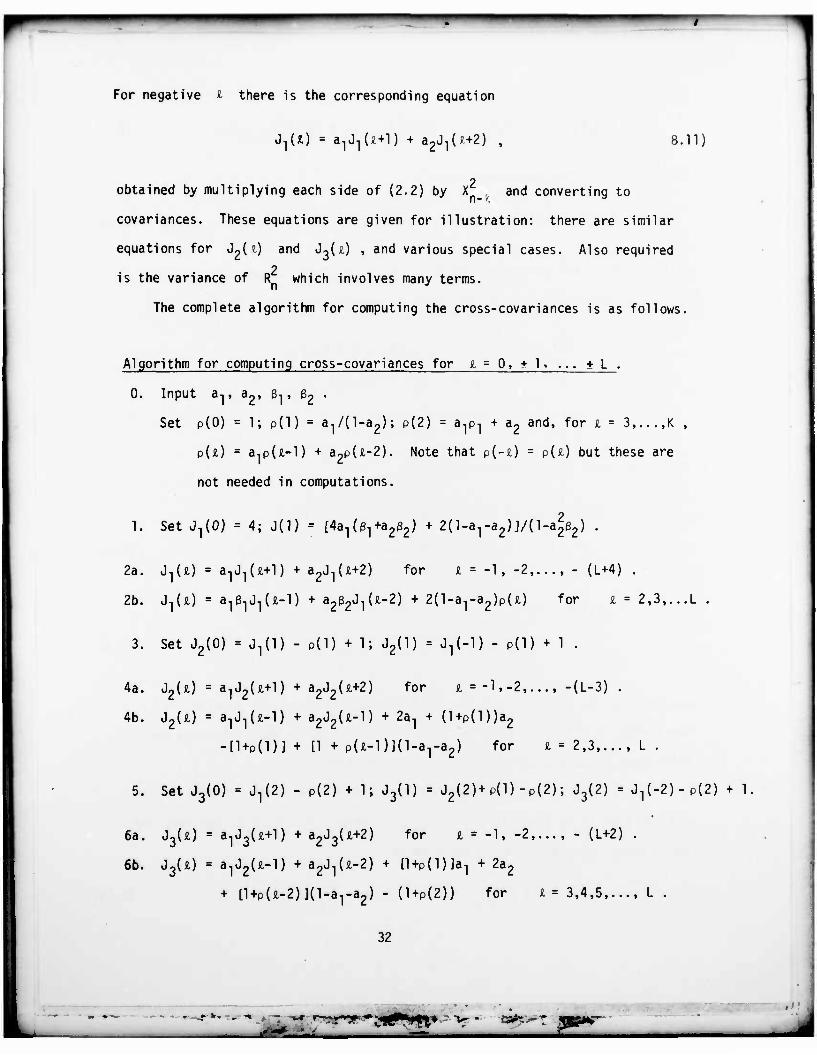
For negative I there is the corresponding equation

JjU) = a1J1(2+l) + agJ^J+2) , 8.11)

obtained by multiplying each side of (2.2) by X _, and converting to

covariances. These equations are given for illustration: there are similar

equations for J2( i) and J^d) , and various special cases. Also required

2 is the variance of R which involves many terms.

The complete algorithm for computing the cross-covariances is as follows,

Algorithm for computing cross-covariances for £ = 0, + 1. ... * L .

0. Input a,, a2, $•,, 32 •

Set p(0) = 1; p(l) = a«/(l-a2h P(2) = a1P1 + a2 and, for £ = 3,...,K ,

P(JI) = a,p(£-l) + a2pU-2). Note that P(-£) = PU) but these are

not needed in computations.

1. Set J}(0) - 4; 0(1) = tfa^+agßg) + 20-aT-a2}]/(l-afß2) .

2a. J,(i) = aÛ+1) + a2J1(£+2) for £ = -1, -2,..., - (L+4) .

2b. JjU) = a^JjU-1) + a2ß2J1(£-2) + 2(l-a1-a2)p(£) for £ = 2,3,...L .

3. Set J2(0) • J^l) - p(l) + 1; J2(l) = J^-l) - p(l) + 1 .

4a. J2U) = aÛ+l) + a2J2()i+2) for 1 = -1, -2,..., -(L-3) .

4b. J2()i) = aÛ-1) + a2J2(a-l) + 2a] + (1+P(l))a2

-[1+P(1)1 + [1 + p(a-l)](l-a1-a2) for £ = 2,3,..., L .

5. Set J3(0) • ^(2) - P(2) + 1; J3(l) = J2(2)+ P(1) - p(2); J3(2) = J^-2) - p(2) + 1

6a. J3U) = a]J3(ji+l) + a2J3()i+2) for t • -1, -2,..., - (L+2) .

6b. J3(ä) • a1J2(£-l) + aÛ-2) + [l+P(l)Ja1 + 2az

+ [l+P(£-2)](l-ara2) - (1+P(2)) for f 3,4,5,..., L .

32

-r *• - -* • - cas-.^T .'•

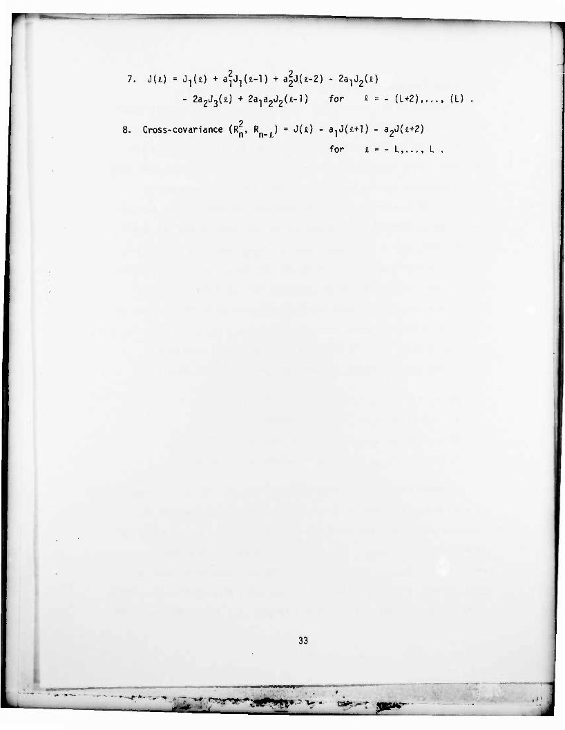
7. JU) = JjU) + a^U-1) + a|j.(l-2) - 23lJ2(0

- 2a2J3(«) + 2a1a2J2(£-l) for l » - (1+2),..., (L)

8. Cross-covariance (R^, R ) = J(jt) - a-,J(ä+1 ) - a2J(«+2)

for t = - L,..., L .

33

* —r *--»•* i. —• r^'^v'iffyH» a**- •- * mil it i

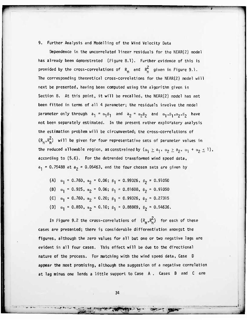
9. Further Analysis and Modelling of the Wind Velocity Data

Dependence in the uncorrelated linear residuals for the NEAR(2) model

has already been demonstrated (Figure 8.1). Further evidence of this is 2

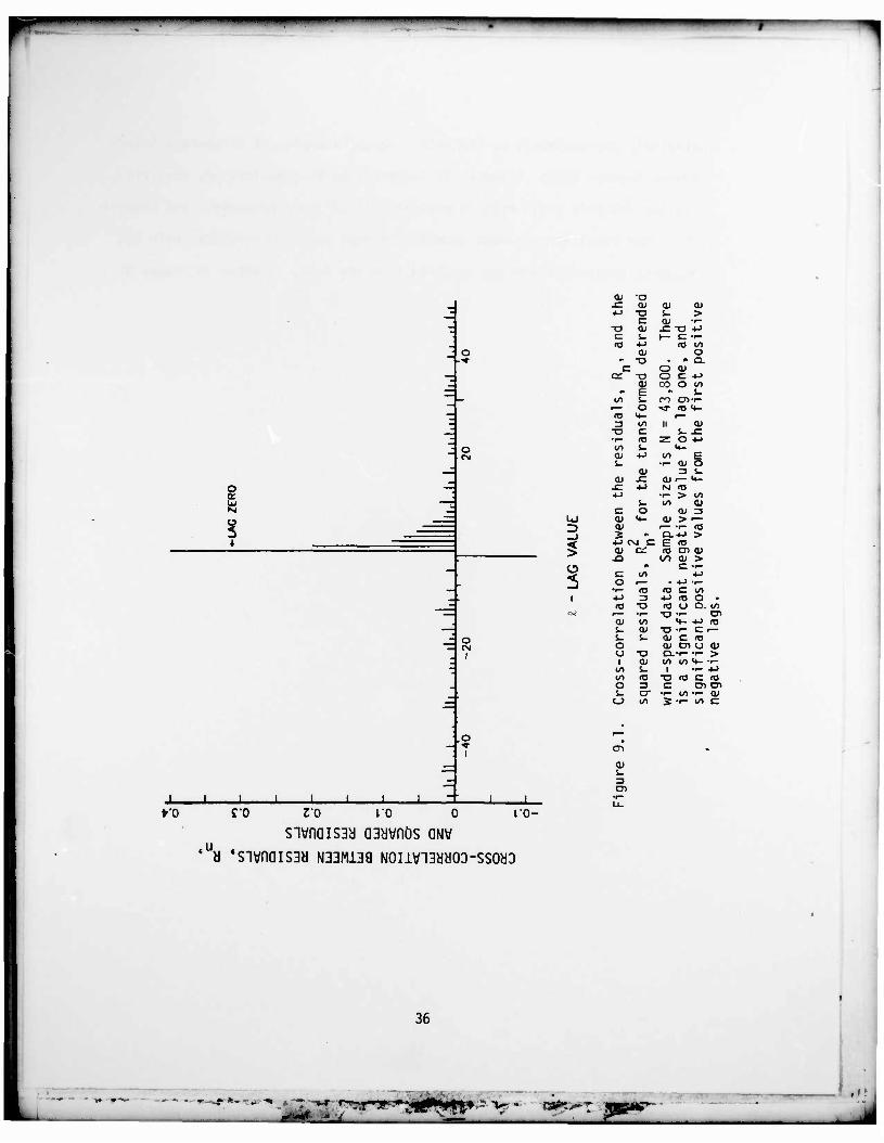
provided by the cross-correlations of R and R~ given in Figure 9.1.

The corresponding theoretical cross-correlations for the NEAR(2) model will

next be presented, having been computed using the algorithm given in

Section 8. At this point, it will be recalled, the NEAR(2) model has not

been fitted in terms of all 4 parameter; the residuals involve the model

parameter only through a-, = a,ß-, and a- = c^ß? ancJ a,,ß,,a„,ß? have

not been separately estimated. In the present rather exploratory analysis

the estimation problem will be circumvented; the cross-correlations of

(R ,R ) will be given for four representative sets of parameter values in

the reduced allowable region, as constrained by (a-, >. a,, a2 > a,, a-, + a« <.!),

according to (5.6). For the detrended transformed wind speed data,

a, = 0.75488 at a2 = 0.05463, and the four chosen sets are given by

(A) cij = 0.760, a2 = 0.06

(B) c^ = 0.925, a2 = 0.06

(C) a] = 0.760, a2 = 0.20

(D) a1 = 0.850, a2 = 0.10

ß1 = 0.99326, ß2 = 0.91050

31 = 0.81608, ß2 = 0.91050

ß1 = 0.99326, ß2 = 0.27315

ß-, = 0.88809, ß2 = 0.54636.

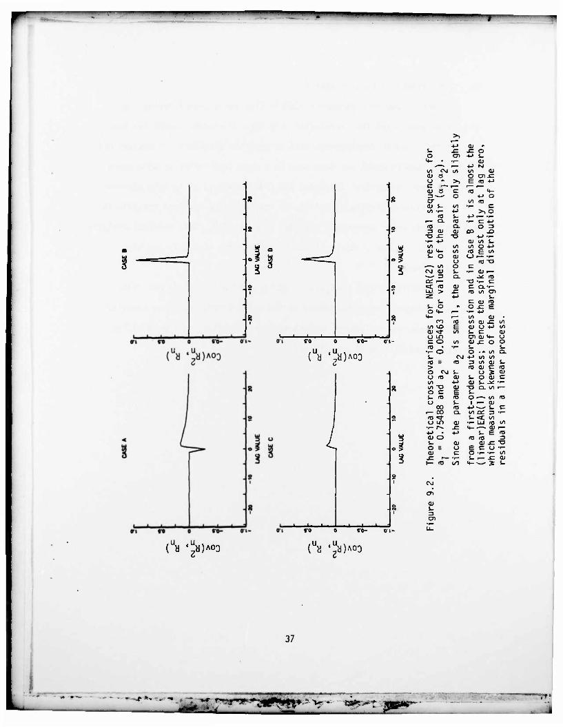
2 In Figure 9.2 the cross-correlations of (Rn»Rn) for each of these

cases are presented; there is considerable differentiation amongst the

figures, although the zero values for all but one or two negative lags are

evident in all four cases. This effect will be due to the directional

nature of the process. For matching with the wind speed data, Case D

appear the most promising, although the suggestion of a negative correlation

at lag minus one lends a little support to Case A . Cases B and C are

34

"H

definitely unsympathetic to the data. Hence, a choice of parameters inter-

mediate between Cases A and D is suggested by this exploratory analysis.

A fuller analysis would require estimates of all four parameters and compari-

son of the resulting residual-squared residual cross-correlations with the

estimated cross-correlations obtained from the data, as shown in Figure 9.1.

35

a*s*r

2 •z

o

~

-; o CM

o —

s

O

1

—

•

.o 1

S JZ

1 I 1 .... 1 1 111- 1 1

O) •o -c T3 s- >

C CD •r- •o Ol .c -o 4-> e s_ t— c •r— ro

CD IO Ul

O p T7 * Q. B O <D

CS -o O C 4-1 CD CO o Ul

m E • (. U7 c ro en *p* ^~ o «3- «3 <4- 13 l*- i—

3 Ul ii Ul s- <*- 01 4-> Ul E s- •r- CD O

01 3 t» CD -C CD i— <«-. -c •*-> M «3 +J •l- > Ul

1- ul 01 c o CD 3

Ul 01 <4- CD > ^- o 0) i-~ *r— IO _J a * 0.-l-> > s +J CM C E iO

CD Cl ra CJl CD -O (•1 CD >

§ •1 C •r-

e l/l +J o ^~ • -t-> •p""

•i— •o «3 C Ul 1 4-> 3 ••-> 10 O •

ID 13 10 O O. Ul erf ^~ •7— -O -r- Ol

CD Ul ••- -<-> 03 i- CD "O 1- C i— i. s- CD C IO O CD Ol l_> 01 u "O CL-^- T> > i (11 Ul Ul <4- -r-

ui i- 1 •r- 4-> ui fO "O (O C IO O 3 s en en (. cr •r- ul •I— CD <_> i/) *•*- Ul C

Ol

2! en

ro co zo ro o sivnaiS3cj a3cjvnös aw

10-

.u a *S1VnaiS3cJ N33M139 N0U\n3HH0D-SS0H3

36

-r *•• •• - -* - ^^^rrn^Wr-1 •Vr- »*, y

•

-«

i * . S

• • i CO TO- 01

(uy '"U)AOO

/

S- -C -C o o en •M s_

<+- • *r— 01 r— •»-> M

to CM tO to 01 0) a o enr o " >> E ro +-> c ^» r^ ^• ^~ 01 d C f0 <+-

_ 3 «*-^ o •t-> O 6 cr to ro

Oi i- tO •<— c CO •r— 4-> >> o

13 S- •t-> r— 'f— r— CL (O •f— c •»-> ro a. O 3 - 3 o> d) co JD

TJ x: T3 •!-> t- •r— 4-> cu to S-

u (/> to to O -t-> 3 01 4- to ro E ">

. * s_ O a> <_> r— "^ o > u ro T3

s ^—^ V) o c C\J 0) s- •r— 0) l— ^w^ 3 CL .* ro CC r— -a •i- c

3 <t (O 0) c Q.-I- 1 >

S- 4->

ro to CJ1 i-

cu ro s_ o •» O x: E O 4- r— •r— ••->

g M- f— to 0J ro (O to cu x: to

•/) tO E cu <_> +J to O) «3- to s- e 01 O in cn Ol <*- o - c o to 5) x: o o (O • •r— s- s_ *^- o o •* to a. s_ CM •!-> to to ro ii (O 13 to a> s- > ro ai c ro O C\J s- <J 2 cu o (O o> s- O 01 c l/l +-> cu i~ JK: • i—

g to T3 cu TD Q. 10 I—

o c E s- s- (O ro o «—« to ro u s_ 1 l— 01

cx> IO +•> -— s. B r— CO a. to a: 3 •r—

B ro «3- (. <: to o LO cu -(— UJ ro to •^ r» _c ti- ^ Ol i

+J • +-> S- E ro

3 tu o ro ro 3

o£ t_ cu 0) sz TJ o II o E c o •#"

3 a> c O •^ *r— to

_£= r— •#" S- r- x: CU 1— ro </l *. •— s s-

CO TO-

("b *^)A°3 ("« (^)AO0

CNJ

CD

Ol

37

»^rrr^ -• "Vr - 13»*!:>ft

•—

10. Conclusions and Further Analysis

The very broad four parameter NEAR(2) time series model having expo-

nential marginals and the correlation structure of an AR(2) model has been

established; further developments will be reported elsewhere. A preliminary

fit of the NEAR(2) model has been made to a very long series of wind speed

data, the data having been detrended and transformed so as to have exponen-

tially distributed marginals; utility of the suggested residual analysis in

probing higher order dependence has been demonstrated. This residual analysis

has been based on the cross-correlations between the residuals and the

squared-residuals.

An extension to this analysis using reversed residuals is possible;

more of the higher order dependency of the NEAR(2) model would be revealed

and this would enable further aspects of its suitability of the model for

the wind speed data to be ascertained.

38

"•"•• —•"•"

BIBLIOGRAPHY

Gaver, D. P. and Lewis, P. A. W. (1980). First-order autoregressive Gamma sequences and point processes. Adv. Appl. Prob., 12^, No. 3, 727-745.

Granger, C. W. and Andersen, A. P. (1978). An Introduction to Bilinear Time Series Models. Gottinger: Vandenhoeck and Ruprecht.

Jacobs, P. A. and Lewis, P. A. W. (1983). Stationary discrete autoregressive- moving average time series generated by mixtures. J. of Time Series Analysis. To appear.

Lawrance, A. J. (1980a). The mixed exponential solution to the first-order autoregressive model. J. Appl. Prob., 12, 522-546.

Lawrance, A. J. (1980b). Some autoregressive models for point processes. Point Processes and Queueing Problems (Colloquia Mathematica Societatis Janos Bolyai 24), ed. P. Bartfai and J. Tomko, North Holland, Amsterdam, 257-275.

Lawrance, A. J. (1982). The innovation distribution of a Gamma distributed autoregressive process. Scand. J. Statist. % 234-236.

Lawrance, A. J. and Lewis, P. A. W. (1980). The exponential autoregressive- moving average EARMA(p.q) process. J. R. Statist. Soc. B, 42, No. 2, 150-161.

Lawrance, A. J. and Lewis, P. A. W. (1981). A new autoregressive time series model in exponential variables (NEAR(l)). Adv. Appl. Prob., 13, 826-845.

Lawrance, A. J. and Lewis, P. A. W. (1982). A mixed exponential time series model. Management Science, 28, No. 9, 1045-1053.

Lewis, P. A. W. (1981). Simple multivariate time series for simulations of complex systems. In Proc. Winter Simulation Conference, eds., T. I. Oren, C. M. Delfosse, C. M. Shube, IEEE Press: New York, 389-390.

Lewis, P. A. W. and Hugus, D. K. (1983). An analysis of 15 years of wind velocity data from ship PAPA. To appear.

Lewis, P. A. W. and Lawrance, A. J. (1983a). A residual analysis for time series with autoregressive correlation structure. To appear.

Lewis, P. A. W. and Lawrance, A. J. (1983b). Simple dependent pairs of exponential and uniform random variables. Operations Research. To appear.

39

^

McKenzie, E. (1982). Product autoregression: A characterization of the Gamma distribution. 19, 463-468.

time series J. Appl. Prob.

McLeod, A. I. and Li, W. K. (1982). Diagnostic checking ARMA time series models using squared-residual autocorrelations. Submitted to J. Time Series Analysis.

Priestley, M. B. (1982). Spectral Analysis and Time Series. Academic Press: New York.

40

* ^-ary-' •Vf* o*s>^ ^J

' "

DISTRIBUTION LIST

Library, Code 0142 Naval Postgraduate School Monterey, CA 93940

Dean of Research Code 012A Naval Postgraduate School Monterey, CA 93940

Library, Code 55 Naval Postgraduate School Monterey, CA 93940

Professor P. A. W. Lewis Code 55 Lw Naval Postgraduate School Monterey, CA 93940

NO. OF COPIES

4

190

41

- v- - ca^^r

stationary exponential time series: … 00 @ nps-55-83-008 naval postgraduate school monterey,...

Documents