statistical analysis of a telephone call center: a …haipeng/publication/callcenter.pdf ·...
TRANSCRIPT

Statistical Analysis of a Telephone Call CenterA Queueing-Science Perspective
Lawrence BROWN Noah GANS Avishai MANDELBAUM Anat SAKOVHaipeng SHEN Sergey ZELTYN and Linda ZHAO
A call center is a service network in which agents provide telephone-based services Customers who seek these services are delayed intele-queues This article summarizes an analysis of a unique record of call center operations The data comprise a complete operationalhistory of a small banking call center call by call over a full year Taking the perspective of queueing theory we decompose the serviceprocess into three fundamental components arrivals customer patience and service durations Each component involves different basicmathematical structures and requires a different style of statistical analysis Some of the key empirical results are sketched along withdescriptions of the varied techniques required Several statistical techniques are developed for analysis of the basic components One ofthese techniques is a test that a point process is a Poisson process Another involves estimation of the mean function in a nonparametricregression with lognormal errors A new graphical technique is introduced for nonparametric hazard rate estimation with censored dataModels are developed and implemented for forecasting of Poisson arrival rates Finally the article surveys how the characteristics deducedfrom the statistical analyses form the building blocks for theoretically interesting and practically useful mathematical models for call centeroperations
KEY WORDS Abandonment Arrivals Call center Censored data Erlang-A Erlang-C Human patience Inhomogeneous Poissonprocess KhintchinendashPollaczek formula Lognormal distribution Multiserver queue Prediction of Poisson rates Queue-ing science Queueing theory Service time
1 INTRODUCTION
Telephone call centers are technology-intensive operationsNevertheless often 70 or more of their operating costs aredevoted to human resources Well-run call centers adhere toa sharply defined balance between agent efficiency and servicequality to do so they use queueing-theoretic models Inputsto these mathematical models are statistics concerning systemprimitives such as the number of agents working the rate atwhich calls arrive the time required for a customer to be servedand the length of time customers are willing to wait on holdbefore they hang up the phone and abandon the queue Out-puts are performance measures such as the distribution of timethat customers wait ldquoon holdrdquo and the fraction of customers thatabandon the queue before being served In practice the numberof agents working becomes a control parameter which can beincreased or decreased to attain the desired efficiencyndashqualitytrade-off
Estimates of these primitives are needed to calibrate queue-ing models and in many cases the models make distribu-tional assumptions concerning the primitives In theory thedata required to validate and properly tune these models shouldbe readily available because computers track and control theminutest details of every callrsquos progress through the system It isthus surprising that operational data collected at an appropriate
Lawrence Brown is Professor Department of Statistics The WhartonSchool University of Pennsylvania Philadelphia PA 19104 (E-mail lbrownwhartonupennedu) Noah Gans is Associate Professor Department of Opera-tions and Information Management The Wharton School University of Penn-sylvania Philadelphia PA 19104 (E-mail ganswhartonupennedu) AvishaiMandelbaum is Professor Faculty of Industrial Engineering and ManagementTechnion Haifa Israel (E-mail avimtxtechnionacil) Anat Sakov is Post-doctoral Fellow Tel-Aviv University Tel-Aviv Israel (E-mail sakovposttauacil) Haipeng Shen is Assistant Professor Department of Statistics Univer-sity of North Carolina Durham NC 27599 (E-mail haipengemailuncedu)Sergey Zeltyn is PhD Candidate Faculty of Industrial Engineering and Man-agement Technion Haifa Israel (E-mail zeltynietechnionacil) LindaZhao is Associate Professor Department of Statistics The Wharton SchoolUniversity of Pennsylvania Philadelphia PA 19104 (E-mail lzhaowhartonupennedu) This work was supported by National Science FoundationDMS-99-71751 and DMS-99-71848 the Sloane Foundation Israeli ScienceFoundation grants 38899 and 12602 the Wharton Financial Institutions Cen-ter and Technion funds for the promotion of research and sponsored research
level of detail have been scarce The data that are typically col-lected and used in the call center industry are simple averagescalculated for the calls that arrive within fixed intervals of timeoften 30 minutes There is a lack of documented comprehen-sive empirical research on call center performance that usesmore detailed data
The immediate goal of our study is to fill this gap In this arti-cle we summarize a comprehensive analysis of operational datafrom a bank call center The data span all 12 months of 1999and are collected at the level of individual calls Our data sourceconsists of more than 1200000 calls that arrived at the centerover the year Of these about 750000 calls terminated in aninteractive voice response unit (IVR or VRU) a type of an-swering machine that allows customers to serve themselvesThe remaining 450000 callers asked to be served by an agentwe have a record of the event-history of each of these calls
This article is an important part of a larger effort to useboth theoretical and empirical tools to better characterize callcenter operations and performance It is an abridged versionof the work of Brown et al (2002a) which provided a morecomplete treatment of the results reported here MandelbaumSakov and Zeltyn (2000) presented a comprehensive descrip-tion of our call-by-call database Gans Koole and Mandelbaum(2003) reviewed queueing and related models of call centersand Mandelbaum (2001) provided an extensive bibliography
11 Queueing Models of Call Centers
The simplest and most widely used queueing model in callcenters is the so-called MMN system sometimes referred toas Erlang-C (Erlang 1911 1917) The MMN model is quiterestrictive It assumes among other things a steady-state en-vironment in which arrivals conform to a Poisson process ser-vice durations are exponentially distributed and customers andservers are statistically identical and act independently of eachother It does not acknowledge among other things customer
copy 2005 American Statistical AssociationJournal of the American Statistical Association
March 2005 Vol 100 No 469 Applications and Case StudiesDOI 101198016214504000001808
36
Brown et al Statistical Analysis of a Telephone Call Center 37
impatience and abandonment behavior time-dependent para-meters customersrsquo heterogeneity or serversrsquo skill levels Anessential task of contemporary queueing theorists is to developmodels that account for these effects
Queueing science seeks to determine which of these ef-fects is most important for modeling real-life situations Forexample Garnett Mandelbaum and Reiman (2002) devel-oped both exact and approximate expressions for MMN + M(also called Erlang-A) systems which explicitly model cus-tomer patience (time to abandonment) as being exponentiallydistributed Empirical analysis can help us judge how wellthe Erlang-C and Erlang-A models predict customer delayswhether or not their underlying assumptions are met
12 Structure of the Article
The article is structured as follows Section 2 describes thecall center under study and its database Each of Sections 3ndash5is dedicated to the statistical analysis of one of the stochasticprimitives of the queueing system Section 3 addresses call ar-rivals Section 4 service durations and Section 5 tele-queueingand customer patience Section 5 also analyzes customer wait-ing times a performance measure deeply intertwined with theabandonment primitive
A synthesis of the primitive building blocks is typicallyneeded for operational understanding Toward this end Sec-tion 6 discusses prediction of the arriving ldquoworkloadrdquo which isessential in practice for setting suitable service staffing levels
Once each of the primitives has been analyzed one canalso attempt to use existing queueing theory or modificationsthereof to describe certain features of the holistic behavior ofthe system Section 7 concludes with analyses of this typeWe validate some classical theoretical results from queueingtheory and refute others
Finally we note that many statistical tests are consideredthroughout the article which raises the problem of multiplicity(Benjamini and Hochberg 1995) When data from call centersare analyzed in support of operational decisions the multiplic-ity problem must be addressed
2 THE CALL CENTER OF BANK ANONYMOUS
The source of our data (Call Center Data 2002) is a smallcall center for one of Israelrsquos banks This center provides sev-eral types of basic services as well as others including stocktrading and technical support for users of the bankrsquos Internetsite On weekdays (SundayndashThursday in Israel) the center isopen from 7 AM to midnight During working hours at most13 regular agents 5 Internet agents and 1 shift supervisor maybe working
A simplified description of the path that each call followsthrough the center is as follows A customer calls one of sev-eral telephone numbers associated with the call center with thenumber depending on the type of service sought Except forrare busy signals the customer is then connected to a VRU andidentifies herself While using the VRU the customer receivesrecorded information both general and customized (eg an ac-count balance) It is also possible for the customer to performsome self-service transactions here and 65 of the bankrsquos cus-tomers actually complete their service via the VRU The other35 indicate the need to speak with an agent If an agent is free
who is capable of performing the desired service then the cus-tomer and the agent are matched to start service immediatelyOtherwise the customer joins the tele-queue
Customers in the tele-queue are nominally served on a first-come first-served (FCFS) basis and customersrsquo positions inqueue are distinguished by the times when they arrive In prac-tice the call center operates a system with two prioritiesmdashhigh and lowmdashand moves high-priority customers up in queueby subtracting 15 minutes from their actual arrival timesMandelbaum et al (2000) compared the behavior of the twopriority groups of customers
While waiting each customer periodically receives informa-tion on his or her progress in the queue More specifically heor she is told the amount of time that the first person in queuehas been waiting as well as his or her approximate location inthe queue The announcement is replayed every 60 seconds orso with music news or commercials intertwined
In each of the 12 months of 1999 roughly 100000ndash120000calls arrived to the system with 65000ndash85000 of these ter-minating in the VRU The remaining 30000ndash40000 calls permonth involved callers who exited the VRU indicating a desireto speak to an agent These calls are the focus of our studyAbout 80 of those requesting service were in fact served andabout 20 were abandoned before being served
Each call that proceeds past the VRU can be thought of aspassing through up to three stages each of which generates dis-tinct data The first of these is the arrival stage which is trig-gered by the callrsquos exit from the VRU and generates a recordof an arrival time If no appropriate server is available then thecall enters the queueing stage Three pieces of data are recordedfor each call that queues the time it entered the queue the timeit exited the queue and the manner in which it exited the queueby being served or abandoning In the last stage service thedata recorded are the starting and ending times of the serviceNote that calls that are served immediately skip the queueingstage and calls that are abandoned never enter the service stage
In addition to these time stamps each call record in our data-base includes a categorical description of the type of servicerequested The main call types are regular (PS in the data-base) stock transaction (NE) newpotential customer (NW)and Internet assistance (IN) Mandelbaum et al (2000) de-scribed the process of collecting and cleaning the data and pro-vided additional descriptive analysis of the data
Over the year two important operational changes occurredFirst in JanuaryndashJuly all calls were served by the same groupof agents but beginning in August Internet (IN) customerswere served by a separate pool of agents Thus in AugustndashDecember the center can be considered to be two separate ser-vice systems one for IN customers and another for all othertypes Second as we discuss in Section 5 one aspect of theservice time data changed at the end of October In severalinstances this articlersquos analyses are based on only the No-vember and December data In other instances we have useddata from AugustndashDecember Given the changes noted earlierthis ensures consistency throughout the manuscript Novemberand December were also convenient because they containedno Israeli holidays In these analyses we also restrict the datato include only regular weekdaysmdashSundayndashThursday 7 AMndashmidnightmdashbecause these are the hours of full operation of the
38 Journal of the American Statistical Association March 2005
center We have performed similar analyses for other parts ofthe data and in most respects the NovemberndashDecember resultsdo not differ noticeably from those based on data from othermonths of the year
3 THE ARRIVAL PROCESS
Figure 1 shows as a function of time of day the averagerate per hour at which calls come out of the VRU These arecomposite plots for weekday calls in November and Decem-ber The plots show calls according to the major call typesThe volume of regular (PS) calls is much greater than that ofthe other three types hence those calls are shown on a sepa-rate plot [These plots were fit using the rootndashunroot methoddescribed by Brown Zhang and Zhao (2001) along with theadaptive free knot spline methodology of Mao and Zhao (2003)For a more precise study of these arrival rates including confi-dence and prediction intervals see our Sec 6 and also Brownet al 2001 2002ab]
Note the bimodal pattern of PS call-arrival times in Figure 1It is especially interesting that IN calls do not show a similarbimodal pattern and in fact have a peak volume after 10 PM(This peak can be partially explained by the fact that Internetcustomers are sensitive to telephone rates which significantlydecrease in Israel after 10 PM and that they also tend to bepeople who stay late)
31 Arrivals Are Inhomogeneous Poisson
Common call center models and practice assume that thearrival process is Poisson with a rate that remains constantfor blocks of time (eg half-hours) with a separate queueingmodel fitted for each block of time A more natural model forcapturing changes in the arrival rate is a time-inhomogeneousPoisson process Following common practice we assume thatthe arrival rate function can be well approximated as beingpiecewise constant
We now construct a test of the null hypothesis that arrivals ofgiven types of calls form an inhomogeneous Poisson processwith piecewise constant rates The first step in constructingour test involves breaking up the duration of a day into rela-tively short blocks of time short enough so that the arrival rate
does not change significantly within a block For conveniencewe used blocks of equal time length L although this equal-ity assumption could be relaxed One can then consider thearrivals within a subset of blocksmdashfor example blocks at thesame time on various days or successive blocks on a given dayThe former case would for example test whether the process ishomogeneous within blocks for calls arriving within the giventime span
Let Tij denote the jth ordered arrival time in the ith blocki = 1 I Thus Ti1 le middot middot middot le TiJ(i) where J(i) denotes the totalnumber of arrivals in the ith block Then define Ti0 = 0 and
Rij = (J(i) + 1 minus j)
(minus log
(L minus Tij
L minus Tijminus1
)) j = 1 J(i)
Under the formal null hypothesis that the arrival rate is constantwithin each given time interval the Rij will be independentstandard exponential variables as we now discuss
Let Uij denote the jth (unordered) arrival time in the ith blockThen the assumed constant Poisson arrival rate within thisblock implies that conditionally on J(i) the unordered ar-rival times are independent and uniformly distributed that is
Uijiidsim U(0L) Note that Tij = Ui( j) It follows that LminusTij
LminusTijminus1
are independent beta(J(i) + 1 minus j1) variables [see eg prob-lem 61433(iii) in Lehmann 1986] A standard change ofvariables then yields the conditional exponentiality of the Rij
given the value of J(i) [One may alternatively base the teston the variables Rlowast
ij = j(minus log TijTij+1
) where j = 1 J(i) andTiJ(i)+1 = L Under the null hypothesis these will also be in-dependent standard exponential variables]
The null hypothesis does not involve an assumption thatthe arrival rates of different intervals are equal or have anyother prespecified relationship Any customary test for the ex-ponential distribution can be applied to test the null hypothe-sis For convenience we use the familiar KolmogorovndashSmirnovtest even though this may not have the greatest possible poweragainst the alternatives of most interest In addition exponen-tial QndashQ plots can be very useful in ascertaining goodness of fitto the exponential distribution
(a) (b)
Figure 1 Arrivals in CallsHour by Time of Day Weekdays in NovemberndashDecember (a) PS calls (b) IN NW and NE calls
Brown et al Statistical Analysis of a Telephone Call Center 39
Brown et al (2002a) presented quantile plots for a few appli-cations of this test For the PS data we found it convenient touse L = 6 minutes For the other types we use L = 60 minutesbecause these calls involved much lower arrival rates
We omit the plots here to save space and because theydemonstrate only minor deviations from the ideal straight-linepattern One example involves arrival times of the PS calls ar-riving between 1112 AM and 1118 AM on all weekdays in No-vember and December A second example involves arrival ofIN calls on Monday November 23 from 7 AM to midnightThis was a typical midweek day in our dataset
For both of the examples the null hypothesis is not rejectedand we conclude that their data are consistent with the assump-tion of an inhomogeneous Poisson process for the arrival ofcalls The respective KolmogorovndashSmirnov statistics have val-ues K = 0316 ( p value asymp 8 with n = 420) and K = 0423( p value asymp 9 with n = 172) These results are typical of thosethat we obtained from various selections of blocks of the var-ious types of calls involving comparable sample sizes Thusoverall from tests of this nature there is no evidence in thisdataset to reject a null hypothesis that the arrival of calls fromthe VRU is an inhomogeneous Poisson process
As an attempt to further validate the inhomogeneous Pois-son character we applied this method to the 48193 PS calls inNovember and December in 6-minute blocks With this largeamount of data one could expect to detect more than statis-tically negligible departures from the null hypothesis becauseof rounding of times in the data (to the nearest second) andbecause arrival rates are not exactly constant within 6-minutetime spans To compensate for the rounding we ldquounroundedrdquothe data before applying the test by adding independent uni-form (01) noise to each observation (This unrounding didnoticeably improve the fit to the ideal pattern) After theunrounding the resulting KolmogorovndashSmirnov statistic wasK = 009 This is a very small deviation from the ideal never-theless the p value for this statistic with such a large n = 48963is p asymp 00007 [To provide an additional benchmark for evalu-ating the (lack of ) importance of this value we note that thissame statistic with n asymp 22000 would have had p value asymp 05which is just acceptable]
4 SERVICE TIME
The goal of a visit to the call center is the service itself Ta-ble 1 summarizes the mean standard deviation (SD) and me-dian service times for the four types of service of main interestThe very few calls with service times gt1 hour were not consid-ered (ie we treat them as outliers) IN calls has little effect onthe numbers IN calls have the longest service times with stocktrading (NE) service calls next Potential customers (NW) havethe shortest service time (which is consistent with the nature ofthese calls) An important implication is that the workload that
Internet consultation imposes on the system is greater than itsshare in terms of percent of calls In earlier work (Brown et al2002a) we also verified that the full cumulative distributions ofthe service times are stochastically ordered in the same fashionas the means in Table 1
41 Very Short Service Times
Figure 2 shows histograms of the combined service times forall types of service for JanuaryndashOctober and for NovemberndashDecember These plots resemble those for PS calls alonebecause the clear majority of calls are for PS We see that inthe first 10 months of the year the percentage of calls with ser-vice lt10 seconds was larger than the percentage at the end ofthe year (7 vs 2)
Service times lt10 seconds are questionable And indeed themanager of the call center discovered that short service timeswere primarily caused by agents who simply hung up on cus-tomers to obtain extra rest time (The phenomenon of agentsldquoabandoningrdquo customers is not uncommon it is often due todistorted incentive schemes especially those that overempha-size short average talk-time or equivalently the total numberof calls handled by an agent) The problem was identified andsteps were taken to correct it in October 1999 For this reasonin the later analysis of service times we focus on data from No-vember and December Suitable analyses can be constructed forthe entire year by using a mixture model or in a somewhat lesssophisticated manner by deleting from the service time analy-sis all calls with service times lt10 seconds
42 On Service Times and Queueing Theory
Most applications of queueing theory to call centers as-sume exponentially distributed service times as their defaultThe main reason for this is the lack of empirical evidence tothe contrary which leads one to favor convenience Indeedmodels with exponential service times are amenable to analy-sis especially when combined with the assumption that arrivalprocesses are homogeneous Poisson processes This is the rea-son that MMN is the prevalent model used in call centerpractice
In more general queueing formulas the service time oftenaffects performance measures through its squared coefficientof variation C2
s = σ 2s E2(S) E(S) is the average service time
and σs is its standard deviation For example a common use-ful approximation for the average waiting time in an MGNmodel (Markovian arrivals generally distributed service timesn servers) is given by
E[Wait for MGN] asymp E[Wait for MMN] times (1 + C2s )
2(1)
(see Sze 1984 Whitt 1993) Note that for large call centers thisformula must be used with care as discussed by Mandelbaum
Table 1 Service Time by Type of Service Truncated at 1 Hour NovemberndashDecember
Regular service Potential customers Internet consulting Stock tradingOverall (PS) (NW) (IN) (NE)
Mean 201 179 115 401 270SD 248 189 146 473 303Median 124 121 73 221 175
40 Journal of the American Statistical Association March 2005
(a) (b)
Figure 2 Distribution of Service Time (a) JanuaryndashOctober (mean 185 SD 238) (b) NovemberndashDecember (mean 200 SD 249)
and Schwartz (2002) Thus average wait with general servicetimes is multiplied by a factor of (1 + C2
s )2 relative to the waitunder exponential service times For example if service timesare in fact exponential then the factor is 1 Deterministic ser-vice times halve the average wait of exponential In our datathe observed factor is (1 + C2
s )2 = 126
43 Service Times Are Lognormal
Looking at Figure 2 we see that the distribution of servicetimes is clearly not exponential as is assumed by standardqueueing theory In fact after separating the calls with veryshort service times our analysis reveals a remarkable fit to thelognormal distribution
Figure 3(a) shows the histogram of log(service time) for No-vember and December in which the short service phenomenonwas absent or minimal Superimposed is the best fitted normal
density as provided by Brown and Hwang (1993) Figure 3(b)shows the lognormal QndashQ plot of service time This does anamazingly good imitation of a straight line Nevertheless theKolmogorovndashSmirnovtest decisively rejects the null hypothesisof exact lognormality (The KolmogorovndashSmirnov statistic hereis K = 020 This is quite small but still much larger than thevalue of K = 009 that was attained for a similarly large sam-ple size in the inhomogeneous Poisson test of Sec 4) We onlyprovide the graphs to qualitatively support our claim of lognor-mality Thus the true distribution is very close to lognormal butis not exactly lognormal (The most evident deviation is in theleft tail of the histogram where both a small excess of observa-tions is evident and the effect of rounding to the nearest secondfurther interferes with a perfect fit) This is a situation wherea very large sample size yields a statistically significant resulteven though there is no ldquopractical significancerdquo
(a) (b)
Figure 3 Histogram (a) and QndashQ Plot (b) of log(service time) NovemberndashDecember
Brown et al Statistical Analysis of a Telephone Call Center 41
After excluding short service times the strong resemblanceto a lognormal distribution also holds for all other monthsIt also holds for various types of callers even though the para-meters depend on the type of call This means that in this casea mixture of lognormals is empirically lognormal even thoughmathematically this cannot exactly hold (See Mandelbaumet al 2000 where the phenomenon is discussed in the contextof the exponential distribution) Brown and Shen (2002) gavea more detailed analysis of service times
Lognormality of processing times has been occasionallyrecognized by researchers in telecommunications and psychol-ogy Bolotin (1994) gave empirical results suggesting thatthe distribution of the logarithm of call duration is normalfor individual telephone customers and a mixture of normalsfor ldquosubscriber-linerdquo groups Ulrich and Miller (1993) andBreukelen (1995) provided theoretical arguments for the log-normality of reaction times using models from mathematicalpsychology Mandelbaum and Schwartz (2000) used simula-tions to study the effect of lognormally distributed service timeson queueing delays
44 Regression of log(service times) on Time of Day
The important implication of the excellent fit to a lognormaldistribution is that we can apply standard techniques to regresslog(service time) on various covariates such as time of day Forexample to model the mean service time across time of daywe can first model the mean and variance of the log(servicetime) across time of day then transform the result back to theservice time scale [Shen (2002) gave a detailed analysis of ser-vice times against other covariates such as the identities of indi-vidual agents (servers) as well as references to other literatureinvolving lognormal variates]
Let S be a lognormally distributed random variable withmean ν and variance τ 2 Then Y = log(S) will be a normalrandom variable with some mean micro and variance σ 2 It iswell known that ν = emicro+σ 22 This parameter (rather than micro ormicro + σ 22) is the primitive quantity that appears in calculationsof offered load as in Section 7 To provide a confidence intervalfor ν we need to derive confidence intervals for micro and σ 2 ormore precisely for micro + σ 22
For our call center data let S be the service time of a calland let T be the corresponding time of day at which the call be-gins service Let SiTin
i=1 be a random sample of size n fromthe joint distribution of ST and sorted according to Ti ThenYi = log(Si) will be the log(service time) of the calls which are(approximately) normally distributed conditional on Ti We canfit a regression model of Yi on Ti as Yi = micro(Ti)+σ(Ti)εi whereεi|Ti are iid N(01)
441 Estimation of micro(middot) and σ 2(middot) If we assume thatmicro(middot) has a continuous third derivative then we can use lo-cal quadratic regression to derive an estimate for micro(middot) (seeLoader 1999) Suppose that micro(t0) is a local quadratic estimatefor micro(t0) Then an approximate 100(1 minus α) confidence in-terval for micro(t0) is micro(t0) plusmn zα2semicro(t0) where semicro(t0) is thestandard error of the estimate of the mean at t0 from the localquadratic fit
Our estimation of the variance function σ 2(middot) is a two-step procedure In the first step we regroup the observa-tions TiYin
i=1 into consecutive nonoverlapping pairs T2iminus1
Y2iminus1 T2iY2in2i=1 The variance at T2i σ 2(T2i) is estimated
by a squared pseudoresidual D2i of the form (Y2iminus1 minus Y2i)22
a so-called ldquodifference-basedrdquo estimate The difference-basedestimator that we use here is a simple one that suffices for ourpurposes In particular our method yields suitable confidenceintervals for estimation of σ 2 More efficient estimators mightimprove our results slightly There are many other difference-based estimators in the literature (see Muumlller and Stadtmuumlller1987 Hall Kay and Titterington 1990 Dette Munk andWagner 1998 Levins 2002)
In the second step we treat T2iD2in2i=1 as our ob-
served data points and apply local quadratic regression to ob-tain σ 2(t0) Part of our justification is that under our modelthe D2irsquos are (conditionally) independent given the T2irsquosA 100(1 minusα) confidence interval for σ 2(t0) is approximatelyσ 2(t0) plusmn zα2seσ 2(t0)
Note that we use zα2 rather than a quantile from a chi-squared distribution as the cutoff value when deriving the fore-going confidence interval Given our large dataset the degreesof freedom are large and a chi-squared distribution can be wellapproximated by a normal distribution
442 Estimation of ν(middot) We now use micro(t0) and σ 2(t0)to estimate ν(t0) as emicro(t0)+σ 2(t0)2 Given that the estimationmethods used for micro(t0) and σ 2(t0) micro(t0) and σ 2(t0) are as-ymptotically independent we have
se(micro(t0) + σ 2(t0)2
) asympradic
semicro(t0)2 + seσ 2(t0)24
When the sample size is large we can assume that micro(middot) +σ 2(middot)2 has an approximately normal distribution Then thecorresponding 100(1 minus α) confidence interval for ν(t0) is
exp((
micro(t0) + σ 2(t0)2) plusmn zα2
radicsemicro(t0)2 + seσ 2(t0)24
)
443 Application and Model Diagnostics In the analysisthat follows we apply the foregoing procedure to the weekdaycalls in November and December The results for two interest-ing service types are shown in Figure 4 There are 42613 PScalls and 5066 IN calls To produce the figures we use thetricube function as the kernel and nearest-neighbor type band-widths The bandwidths are automatically chosen via cross-validation
Figure 4(a) shows the mean service time for PS calls asa function of time of day with 95 confidence bands Notethe prominent bimodal pattern of mean service time across theday for PS calls The accompanying confidence band shows thatthis bimodal pattern is highly significant The pattern resemblesthat for arrival rates of PS calls (see Fig 1) This issue was dis-cussed further by Brown et al (2002a)
Figure 4(b) plots an analogous confidence band for IN callsOne interesting observation is that IN calls do not show a sim-ilar bimodal pattern We do see some fluctuations during theday but these are only mildly significant given the wide con-fidence band Also notice that the entire confidence band forIN calls lies above that of PS calls This reflects the stochasticdominance referred to in the discussion of Table 1
Standard diagnostics on the residuals reveal a qualitativelyvery satisfactory fit to lognormality comparable with that inFigure 3
42 Journal of the American Statistical Association March 2005
(a) (b)
Figure 4 Mean Service Time (PS) (a) versus Time of Day [95 confidence interval (CI)] (b) Mean Service Time (IN) versus Time of Day(95 CI)
5 WAITING FOR SERVICE OR ABANDONING
In Sections 3 and 4 we characterized two primitives of queue-ing models the arrival process and service times In each casewe were able to directly observe and analyze the primitive un-der investigation We next address the last system primitivecustomer patience and abandonment behavior and the relatedoutput of waiting time Abandonment behavior and waitingtimes are deeply intertwined
There is a distinction between the time that a customer needsto wait before reaching an agent and the time that a customeris willing to wait before abandoning the system The formeris referred to as virtual waiting time because it amounts tothe time that a (virtual) customer equipped with infinite pa-tience would have waited until being served We refer to thelatter as patience Both measures are obviously of great impor-tance but neither is directly observable and hence both mustbe estimated
A well-known queueing-theoretic result is that in heavilyloaded systems (in which essentially all customers wait and noone abandons) waiting time should be exponentially distrib-uted (See Kingman 1962 for an early result and Whitt 2002 fora recent text) Although our system is not very heavily loadedand in our system customers do abandon we find that the ob-served distribution of time spent in the queue conforms verywell to this theoretical prediction (see Brown et al 2002a forfurther details)
51 Survival Curves for Virtual Waiting Timeand Patience
Both times to abandonment and times to service are cen-sored data Let R denote the ldquopatiencerdquo or ldquotime willing towaitrdquo and let V denote the ldquovirtual waiting timerdquo and equipboth with steady-state distributions One actually samplesW = minRV as well as the indicator 1RltV for observ-ing R or V One considers all calls that reached an agent ascensored observations for estimating the distribution of R andvice versa for estimating the distribution of V We make theassumption that (as random variables) R and V are indepen-dent given the covariates relevant to the individual customerUnder this assumption the distributions of R and V (given the
covariates) can be estimated using the standard KaplanndashMeierproduct-limit estimator
One may plot the KaplanndashMeier estimates of the survivalfunctions of R (time willing to wait) V (virtual waiting time)and W = minVR (see Brown et al 2002a) There is a clearstochastic ordering between V and R in which customers arewilling to wait (R) more than they need to wait (V) Thissuggests that our customer population consists of patient cus-tomers Here we have implicitly and only intuitively definedthe notion of a patient customer (To the best of our knowledgesystematic research on this subject is lacking)
We also consider the survival functions of R for differenttypes of service Again a clear stochastic ordering emergesFor example customers performing stock trading (type NE) arewilling to wait more than customers calling for regular services(type PS) A possible empirical explanation for this orderingis that type NE needs the service more urgently This suggestsa practical distinction between tolerance for waiting and loy-altypersistency
52 Hazard Rates
Palm (1953) was the first to describe impatience in terms ofa hazard rate He postulated that the hazard rate of the timewilling to wait is proportional to a customerrsquos irritation due towaiting Aalen and Gjessing (2001) advocated dynamic inter-pretation of the hazard rate but warned against the possibil-ity that the population hazard rate may not represent individualhazard rates
We have found it useful to construct nonparametric estimatesof the hazard rate It is feasible to do so because of the largesample size of our data (about 48000) Figure 5 shows suchplots for R and V
The nonparametric procedure that we use to calculate andplot the figures is as follows For each interval of length δ theestimate of the hazard rate is calculated as
[number of events during (t t + δ]][number at risk at t] times δ
For smaller time values t the numbers at risk and event ratesare large and we let δ = 1 second For larger times when fewer
Brown et al Statistical Analysis of a Telephone Call Center 43
(a) (b)
Figure 5 Hazard Rates for (a) the Time Willing to Wait for PS Calls and (b) Virtual Waiting Time NovemberndashDecember
are at risk we use larger δrsquos Specifically the larger intervals areconstructed to have an estimated expected number of events perinterval of at least four Finally the hazard rate for each intervalis plotted at the intervalrsquos midpoint
The curves superimposed on the plotted points are fitted us-ing nonparametric regression In practice we used LOCFIT(Loader 1999) although other techniques such as kernel proce-dures or smoothing splines would yield similar fits We choosethe smoothing bandwidth by generalized cross-validation(We also smoothly transformed the x-axis so that the obser-vations would be more nearly uniformly placed along that axisbefore producing a fitted curve We then inversely transformedthe x-axis to its original form) We experimented with fittingtechniques that varied the bandwidth to take into account theincreased variance and decreased density of the estimates withincreasing time However with our data these techniques hadlittle effect and thus we do not use here
Figure 5(a) plots the hazard rates of the time willing to waitfor PS calls Note that it shows two main peaks The first peakoccurs after only a few seconds When customers enter thequeue a ldquoplease waitrdquo message as described in Section 2 isplayed for the first time At this point some customers who donot wish to wait probably realize they are in a queue and hangup The second peak occurs at about t = 60 about the time thatthe system plays the message again Apparently the messageincreases customersrsquo likelihood of hanging up for a brief timethereafter an effect that may be contrary to the messagersquos in-tended purpose (or maybe not)
In Figure 5(b) the hazard rate for the virtual waiting times isestimated for all calls (The picture for PS alone is very simi-lar) The overall plot reveals rather constant behavior and indi-cates a moderate fit to an exponential distribution (The gradualgeneral decrease in this hazard rate from about 008 to 005suggests an issue that may merit further investigation)
53 Patience Index
Customer patience on the telephone is important yet it hasnot been extensively studied In the search for a better under-standing of patience we have found a relative definition to beof use Let the means of V and R be mV and mR One can definethe patience index as the ratio mRmV the ratio of the mean
time a customer is willing to wait to the mean time he or sheneeds to wait The justification for calling this a ldquopatience in-dexrdquo is that for experienced customers the time that one needsto wait is in fact that time that one expects to wait Although thispatience index makes sense intuitively its calculation requiresthe application of survival analysis techniques to call-by-calldata Such data may not be available in certain circumstancesTherefore we wish to find an empirical index that will work asan auxiliary measure for the patience index
For the sake of discussion we assume that V and R are in-dependent and exponentially distributed As a consequence ofthese assumptions we can demonstrate that
Patience index= mR
mV= P(V lt R)
P(R lt V)
Furthermore P(V lt R)P(R lt V) can be estimated by (numberserved)(number abandoned) and we define
Empirical index= number served
number abandoned
The numbers of both served and abandoned calls are very easyto obtain from either call-by-call data or more aggregated callcenter management reports We have thus derived an easy-to-calculate empirical measure from a probabilistic perspectiveThe same measure can also be derived using the maximum like-lihood estimators for the mean of the (right-censored) exponen-tial distribution applied separately to R and to V
We can use our data to validate the empirical index as an es-timate of the theoretical patience index Recall however thatthe KaplanndashMeier estimate of the mean is biased when the lastobservation is censored or when heavy censoring is presentNevertheless a well-known property of exponential distribu-tions is that their quantiles are just the mean multiplied bycertain constants and we use quantiles when calculating the pa-tience index In fact because of heavy censoring we sometimesdo not obtain an estimate for the median or higher quantilesTherefore we used first quartiles when calculating the theoret-ical patience index
The empirical index turns out to be a very good estimate ofthe theoretical patience index For each of 68 quarter hours be-tween 7 AM and midnight we calculated the first quartiles ofV and R from the survival curve estimates We then compared
44 Journal of the American Statistical Association March 2005
the ratio of the first quartiles to that of (number of served)to (number of abandoned) The resulting 68 sample pairs hadan R2 of 94 (see Brown et al 2002a for a plot) This resultsuggests that we can use the empirical measure as an index forhuman patience
With this in mind we obtain the following empirical indicesfor regular weekdays in November and December PS = 534NE = 871 NW = 161 and IN = 374 We thus find thatthe NE customers are the most patient perhaps because theirbusiness is the most important to them On the other hand bythis measure the IN customers are less patient than the PS cus-tomers In this context we emphasize that the patience indexmeasures time willing to wait normalized by time needed towait In our case (as previously noted) the IN customers arein a separate queue from that of the PS customers The IN cus-tomers on average are willing to wait slightly longer than the PScustomers (see Brown et al 2002a) However they also need towait longer and overall their patience index is less than that ofthe PS customers
Recall that the linear relationship between the two indicesis established under the assumption that R and V are expo-nentially distributed and independent As Figure 5(a) showshowever the distribution for R is clearly not exponential Sim-ilarly Figure 5(b) shows that V also displays some deviationfrom exponentiality Furthermore sequential samples of V arenot independent of each other Thus we find that the linear rela-tion is surprisingly strong
Finally we note another peculiar observation The line doesnot have an intercept at 0 or a slope of 1 as suggested by theforegoing theory Rather the estimated intercept and slope areminus182 and 135 which are statistically different from 0 and 1We are working on providing a theoretical explanation that ac-counts for these peculiar facts as well as an explanation forthe fact that the linear relationship holds so well even thoughthe assumption of exponentiality does not hold for our data(The assumption of independence of R and V may also bequestionable)
6 PREDICTION OF THE LOAD
This section reflects the view of the operations manager ofa call center who plans and controls daily and hourly staffinglevels Prediction of the system ldquoloadrdquo is a key ingredient inthis planning Statistically this prediction is based on a combi-nation of the observed arrival times to the system (as analyzedin Sec 3) and service times during previous comparable peri-ods (as analyzed in Sec 4)
In the discussion that follows we describe a convenient modeland a corresponding method of analysis that can be used to gen-erate prediction confidence bounds for the load of the systemMore specifically in Section 64 we present a model for pre-dicting the arrival rate and in Section 66 we present a modelfor predicting mean service time In Section 67 we combine thetwo predictions to obtain a prediction (with confidence bounds)for the load according to the method discussed in Section 63
61 Definition of Load
In Section 3 we showed that arrivals follow an inhomoge-neous Poisson process We let j(t) denote the true arrival rateof this process at time t on a day indexed by the subscript j
Figure 1 presents a summary estimate of middot(t) the averageof j(t) over weekdays in November and December
For simplicity of presentation here we treat together allcalls except the IN calls because these were served in a sep-arate system in AugustndashDecember The arrival patterns for theother types of calls appear to be reasonably stable in AugustndashDecember Therefore in this section we use the AugustndashDecember data to fit the arrival parameters To avoid havingto adjust for the short service time phenomenon noted inSection 41 we use only November and December data to fitparameters for service times Also here we consider only reg-ular weekdays (SundayndashThursday) that were not full or partialholidays
Together an arbitrary arrival rate (t) and mean servicetime ν(t) at t define the ldquoloadrdquo at that time L(t) = (t)ν(t)This is the expected time units of work arriving per unit of timea primitive quantity in building classical queueing models suchas those discussed in Section 7
Briefly suppose that one adopts the simplest MMN queue-ing model Then if the load is a constant L over a sufficientlylong period the call center must be staffed according to themodel with at least L agents otherwise the model predictsthat the backlog of calls waiting to be served will explode in anever-increasing queue Typically a manager will need to staffthe center at a staffing level that is some function of Lmdashforexample L + c
radicL for some constant cmdashto maintain satisfac-
tory performance (see Borst Mandelbaum and Reiman 2004Garnett et al 2002)
62 Independence of (t) and ν(t)
In Section 544 we noted a qualitative similarity in the bi-modal pattern of arrival rates and mean service times To tryto explain this similarity we tested several potential explana-tions including a causal dependence between arrival rate andservice times We were led to the conclusion that such a causaldependence is not a statistically plausible explanation Ratherwe concluded that the periods of heavier volume involve a dif-ferent mix of customers a mix that includes a higher populationof customers who require lengthier service The statistical evi-dence for this conclusion is indirect and was reported by Brownet al (2002a) Thus we proceed under the assumption that ar-rival rates and mean service times are conditionally independentgiven the time of day
63 Coefficient of Variation for the Prediction of L(t)
Here we discuss the derivation of approximate confidenceintervals for (t) and ν(t) based on observations of quarter-hour groupings of the data The load L(t) is a product of thesetwo quantities Hence exact confidence bounds are not read-ily available from individual bounds for each of (t) and ν(t)As an additional complication the distributions of the individ-ual estimates of these quantities are not normally distributedNevertheless one can derive reasonable approximate confi-dence bounds from the coefficient of variation (CV) for the es-timate of L
For any nonnegative random variable W with finite posi-tive mean and variance define the CV (as usual) by CV(W) =
Brown et al Statistical Analysis of a Telephone Call Center 45
SD(W)E(W) If U and V are two independent variables andW = UV then an elementary calculation yields
CV(W) =radic
CV2(U) + CV2(V) + CV2(U) middot CV2(V)
In our case U and V correspond to and ν Predictionsfor and ν are discussed in Sections 74 and 76 As notedearlier these predictions can be assumed to be statisticallyindependent Also their CVs are quite small (lt1) Notethat L(t) = (t)ν(t) and using standard asymptotic nor-mal theory we can approximate CV(L)(t) as CV(L)(t) asympradic
CV2()(t) + CV2(ν)(t)This leads to approximate 95 CIs of the form L(t) plusmn
2L(t)CV(L)(t) The constant 2 is based on a standard asymp-totic normal approximation of roughly 196
64 Prediction of (t)
Brown and Zhao (2001) investigated the possibility of mod-eling the parameter as a deterministic function of time of dayday of week and type of customer and rejected such a modelHere we construct a random-effects model that can be used topredict and to construct confidence bands for that predictionThe model that we construct includes an autoregressive featurethat incorporates the previous dayrsquos volume into the predictionof todayrsquos rate
In the model which we elaborate on later we predict thearrival on a future day using arrival data for all days up to thatday Such predictions should be valid for future weekdays onwhich the arrival behavior follows the same pattern as those forthat period of data
Our method of accounting for dependence on time and day ismore conveniently implemented with balanced data althoughit can also be used with unbalanced data For conveniencewe have thus used arrival data from only regular (nonholi-day) weekdays in AugustndashDecember on which there were noquarter-hour periods missing and no obvious gross outliers inobserved quarter-hourly arrival rates This leaves 101 days Foreach day (indexed by j = 1 101) the number of arrivals ineach quarter hour from 7 AMndashmidnight was recorded as Njkk = 1 68 As noted in Section 3 these are assumed to bePoisson with parameter = jk
One could build a fundamental model for the values of
according to a model of the form
Njk = Poisson(jk) jk = Rjτk + εprimejk (2)
where the τkrsquos are fixed deterministic quarter-hourly effects theRjrsquos are random daily effects with a suitable stochastic charac-ter and the εprime
jkrsquos are random errors Note that this multiplicativestructure is natural in that the τkrsquos play the role of the expectedproportion of the dayrsquos calls that fall in the kth interval This isassumed to not depend on the Rjrsquos the expected overall numberof calls per day (We accordingly impose the side condition thatsum
τk = 1)We instead proceed in a slightly different fashion that is
nearly equivalent to (2) but is computationally more convenientand leads to a conceptually more familiar structure The ba-sis for our method is a version of the usual variance-stabilizing
transformation If X is a Poisson(λ) variable then V =radic
X + 14
has approximately mean θ = radicλ and variance σ 2 = 1
4 This is
nearly precise even for rather small values of λ [One insteadcould use the simpler form
radicX or the version of Anscombe
(1948) that hasradic
X + 38 in place of
radicX + 1
4 only numericallysmall changes would result Our choice is based on considera-tions of Brown et al (2001)] Additionally V is asymptoticallynormal (as λ rarr infin) and it makes sense to treat it as such in the
models that follow We thus let Vjk =radic
Njk + 14 and assume the
model
Vjk = θjk + εlowastjk with εlowast
jkiidsim N
(0 1
4
)
θjk = αjβk + εjk (3)
αj = micro + γ Vjminus1+ + Aj
where Aj sim N(0 σ 2A) εjk sim N(0 σ 2
ε ) Vj+ = sumk Vjk and
Aj and εjk are independent of each other and of values of Vjprimekfor jprime lt j Note that αj is a random effect in this model Further-more the model supposes a type of first-order autoregressivestructure on the random daily effects The correspondence be-tween (2) and (3) implies that this structure is consistent withan approximate assumption that
Rj =(
γsum
k
radicNjminus1k + 1
4+ Aj
)2
The model is thus not quite a natural one in terms of Rj but itappears more natural in terms of the Vjk in (3) and is computa-tionally convenient
The parameters γ and βk need to be estimated as do micro σ 2A
and σ 2ε We impose the side condition
sumβ2
k = 1 which cor-responds to the condition
sumτk = 1 The goal is then to de-
rive confidence bounds for θjk = radicjk in (3) and squaring the
bounds yields corresponding bounds for jkThe parameters in the model (3) can easily be estimated by
a combination of least squares and method of moments Beginby treating the αjrsquos as if they were fixed effects and using leastsquares to fit the model
Vjk = αjβk + (εjk + εlowastjk)
This is an easily solved nonlinear least squares problemIt yields estimates αj βk and σ 2 where the latter estimate isthe mean squared error from this fit Then σ 2
ε can be estimatedby method of moments as
σ 2ε = σ 2 minus 1
4
Then use the estimates αj to construct the least squares esti-mates of these parameters that would be appropriate for a linearmodel of the form
αj = micro + γ Vjminus1+ + Aj (4)
This yields least squares estimates micro and γ and the standardmean squared error estimator σ 2
A for the variance of AjThe estimates calculated from our data for the quantities re-
lated to the random effects are
micro = 9788 γ = 6784
(with corresponding R2 = 501)
σ 2A = 4083 σ 2
ε = 1078 (because σ 2 = 3578)
(5)
46 Journal of the American Statistical Association March 2005
The value of R2 reported here is derived from the estimationof γ in (3) and it measures the reduction in sum of squared er-ror due to fitting the αj by this model which captures the pre-vious dayrsquos call volumes Vjminus1+ The large value of R2 makesit clear that the introduction of the autoregressive model notice-ably reduces the prediction error (by about 50) relative to thatobtainable from a model with no such component that is onein which a model of the form (3) holds with γ = 0
For a prediction13
k of tomorrowrsquos value of k at a partic-ular quarter hour (indexed by k) one would use the foregoingestimates along with todayrsquos value of V+ From (3) it followsthat tomorrowrsquos prediction is
13
θ k = βk(γ V+ + micro) (6)
as an estimate of
θk = βk(γ V+ + micro + A) + ε (7)
where A sim N(0 σ 2A) and ε sim N(0 σ 2
ε ) are independent Thevariance of the term in parentheses in (7) is the predictionvariance of the regression in (6) Denote this by pred var(V+)The coefficient of variation of βk turns out to be numericallynegligible compared with other coefficients of variation in-volved in (6) and (7) Hence
var(13
θ k) asymp β2k times pred var(V+) + σ 2
ε (8)
These variances can be used to yield confidence intervals forthe predictions of θk The bounds of these confidence intervalscan then be squared to yield confidence bounds for the predic-tion of k Alternatively one may use the convenient formulaCV(
13
θ 2k) asymp 2 times CV(
13
θ k) and produce the corresponding confi-dence intervals (see Brown et al 2002a for such a plot)
We note that the values of CV(13
θ 2k) here are in the range of 25
(for early morning and late evening) down to 16 (for mid-day) Note also that both parts of (8) are important in determin-ing variability the values of var(
13
θ k) range from 14 (for earlymorning and late evening) up to 27 (for midday) The fixed partof this is σ 2
ε = 11 and the remainder results from the first partof (8) which reflects the variability in the estimate of the dailyvolume figure A in (3)
Correspondingly better estimates of daily volume (perhapsbased on covariates outside our dataset) would considerablydecrease the CVs during midday but would not have much ef-fect on those for early morning and late evening [Incidentallywe tried including day of the week an additional covariate inthe model (3) but with the present data this did not noticeablyimprove the resulting CVs]
A natural suggestion would be to use a nonparametric modelfor the curve (t) in place of the binned model in (2) and (3)This suggestion is appealing and we plan to investigate itHowever we have not so far succeeded in producing a nonpara-metric regression analysis that incorporates all of the features ofthe foregoing model and also provides theoretically unbiasedprediction intervals
The preceding model includes several assumptions of nor-mality These can be empirically checked in the usual way byexamining residual plots and QndashQ plots of residuals All of therelevant diagnostic checks showed good fit to the model For ex-ample the QndashQ plots related to A and ε support the normality
assumptions in the model According to the model the residualscorresponding to εjk also should be normally distributed TheQndashQ plot for these residuals has slightly heavier-than-normaltails but only 5 (out of 6868) values seem to be heavily ex-treme These heavy extremes correspond to quarter-hour peri-ods on different days that are noticeably extreme in terms oftheir total number of arrivals
65 Prediction of ν(t)
In this section we also model the service time according toquarter-hour intervals This allows us to combine (in Sec 66)the estimates of ν(t) derived here with the estimates of (t)derived in Section 64 and to obtain rigorously justifiablebias-free prediction confidence intervals In other respects themodel developed in this section resembles the nonparametricmodel of Section 44
We use weekday data from only November and DecemberThe lognormality discussed in Section 43 allows us to modellog(service times) rather than service times Let Yjkl denote thelog(service time) of the lth call served by an agent on day jj = 1 44 in quarter-hour intervals k k = 1 68 In totalthere are n = 57152 such calls (We deleted the few call recordsshowing service times of 0 or gt 3600 seconds) For purposesof prediction we will ultimately adopt a model similar to thatof Section 44 namely
Yjkl = micro + κk + εjkl εjkl sim N(0 σ 2k ) (indep) (9)
Before adopting such a model we investigated whether thereare day-to-day inhomogeneities that might improve the predic-tion model We did this by adding a random-day effect to themodel in (9) The larger model had a partial R2 = 005 This isstatistically significant ( p value lt 0001) due to the large sam-ple size but it has very little numerical importance We alsoinvestigated a model that used the day as an additional factorbut found no useful information in doing so Hence in what fol-lows we use model (9)
The goal is to produce a set of confidence intervals (or corre-sponding CVs) for the parameter
νk = exp
(micro + κk + σ 2
k
2
) (10)
The basis for this is contained in Section 44 except that herewe use estimates from within each quarter-hour time periodrather than kernel-smoothed estimates This enables us to ob-tain rigorously justifiable bias-free prediction confidence inter-vals The most noticeable difference is that the standard errorof σ 2
k is now estimated by
seσ 2k
asympradic
2
nk minus 1S2
k (11)
where nk denotes the number of observations within the quarterhour indexed by k and S2
k denotes the corresponding sam-ple variance from the data within this quarter hour This es-timate is motivated by the fact that if X sim N(microσ 2) thenvar((X minusmicro)2) = 2σ 4 (see Brown et al 2002a for a plot of theseprediction intervals)
CVs for these estimates can be calculated from the approxi-
mate (Taylor series) formula CVlowast(νk) asymp CV(micro+ κk + σ 2k2 ) (The
Brown et al Statistical Analysis of a Telephone Call Center 47
Figure 6 95 Prediction Intervals for the Load L Following a DayWith V+ = 340
intervals νk plusmn 196 times νk times CVlowast agree with the foregoing towithin 1 part in 200 or better) The values of CV here rangefrom 03 to 08 These are much smaller than the correspondingvalues of CVs for estimating (t) Consequently in producingconfidence intervals for the load L(t) the dominant uncertaintyis that involving estimation of (t)
66 Confidence Intervals for L(t)
The confidence intervals can be combined as described inSection 63 to obtain confidence intervals for L in each quarter-hour period Care must be taken to first convert the estimates of and ν to suitable matching units Figure 6 shows the result-ing plot of predicted load on a day following one in which thearrival volume had V+ = 340
The intervals in Figure 6 are still quite wide This reflects thedifficulty in predicting the load at a relatively small center suchas ours We might expect predictions from a large call center tohave much smaller CVs and we are currently examining datafrom such a large center to see whether this is in fact the caseOf course inclusion (in the data and corresponding analysis) ofadditional informative covariates for the arrivals might improvethe CVs in a plot such as Figure 6
7 SOME APPLICATIONS OF QUEUEING SCIENCE
Queueing theory concerns the development of formal math-ematical models of congestion in stochastic systems such astelephone and computer networks It is a highly developed dis-cipline that has roots in the work of A K Erlang (Erlang1911 1917) at the beginning of the twentieth century Queueingscience as we view it is the theoryrsquos empirical complementit seeks to validate and calibrate queueing-theoretic models viadata-based scientific analysis In contrast to queueing theoryhowever queueing science is only starting to be developedAlthough there exist scattered applications in which the as-sumptions of underlying queueing models have been checkedwe are not aware of previous systematic effort to validatequeueing-theoretic results
One area in which extensive work has been donemdashand hasmotivated the development of new theorymdashinvolves the arrivalprocesses of Internet messages (or message packets) (see egWillinger Taqqu Leland and Wilson 1995 Cappe Moulines
Pesquet Petropulu and Yang 2002 and the references therein)These arrivals have been found to involve heavy-tailed distrib-utions andor long-range dependencies (and thus differ qualita-tively from the results reported in our Sec 3)
In this section we use our call center data to produce two ex-amples of queueing science In Section 71 we validate (andrefute) some classical theoretical results In Section 72 wedemonstrate the robustness (and usefulness) of a relativelysimple theoretical model namely the MMN+M (Erlang-A)model for performance analysis of a complicated realitynamely our call center
71 Validating Classical Queueing Theory
We analyze two congestion laws first the relationship be-tween patience and waiting which is a byproduct of Littlersquoslaw (Zohar Mandelbaum and Shimkin 2002 Mandelbaum andZeltyn 2003) and then the interdependence between servicequality and efficiency as it is manifested through the classicalKhintchinendashPollaczek formula (see eg eq 568 in Hall 1991)
711 On Patience and Waiting Here we consider the re-lationship between average waiting time and the fraction ofcustomers that abandon the queue To do so we compute thetwo performance measures for each of the 3867 hourly in-tervals that constitute the year Regression then shows that astrong linear relationship exists between the two with a valueof R2 = 875
Indeed if W is the waiting time and R is the time a customeris willing to wait (referred to as patience) then the law
Abandonment = E(W)
E(R)(12)
is provable for models with exponential patience like those ofBaccelli and Hebuterne (1981) and Zohar et al (2002) How-ever exponentiality is not the case here (see Fig 5)
Thus the need arises for a theoretical explanation of why thislinear relationship holds in models with generally distributedpatience Similarly the identification and analysis of situationsin which nonlinear relationships arise remains an important re-search question [Motivated by the present study Mandelbaumand Zeltyn (2003) pursued both directions]
Under the hypothesis of exponentiality we use (12) to es-timate the average time that a customer is willing to wait ina queue an absolute measure of customer patience (Comparethis with the relative index defined in Sec 53) From the inverseof the regression-line slope we find that the average patience is446 seconds in our case
712 On Efficiency and Service Levels As fewer agentscope with a given workload operational efficiency increasesThe latter is typically measured by the system (or agentsrsquo) ldquooc-cupancyrdquo the average utilization of agents over time Formallythis is defined as
ρ = λeff
Nmicro (13)
where λeff is the effective arrival rate (namely the arrival rateof customers who get served) micro is the service rate [E(S) = 1micro
is the average service time] and N is number of active agentseither serving customers or available to do so Thus the staffing
48 Journal of the American Statistical Association March 2005
Figure 7 Agentsrsquo Occupancy versus Average Waiting Time
level N is required to calculate agentsrsquo occupancy Neither oc-cupancies nor staffing levels are explicit in our database how-ever so we derive indirect measures of these from the availabledata (see Brown et al 2002a for details)
The three plots of Figure 7 depict the relationship betweenaverage waiting time and agentsrsquo occupancy The first plotshows the result for each of the 3867 hourly intervals over theyear The second and third plots emphasize the patterns by ag-gregating the data (The hourly intervals were ordered accord-ing to their occupancy and adjacent groups of 45 were thenaveraged together)
The classical KhintchinendashPollaczek formula suggests the ap-proximation
E(W) asymp 1
N
ρ
1 minus ρ
1 + C2s
2E(S) (14)
which is a further approximation of (1) (see eg Whitt 1993)Here Cs denotes the coefficient of variation of the service timeand ρ denotes the agentsrsquo occupancy
The third plot of Figure 7 tests the applicability of theKhintchinendashPollaczek formula in our setting by plottingN middot E(W)E(S) versus ρ(1 minus ρ) To check whether the twoplots exhibit the linear pattern implied by (14) we display anaggregated version of the data as a scatterplot on a logarithmicscale This graph pattern is not linear This can be explained bythe fact that classical versions of KhintchinendashPollaczek formulaare not appropriate for queueing systems with abandonment
Note that queueing systems with abandonment usually giverise to dependence between successive interarrival times ofserved customers as well as between interarrival times ofserved customers and service times For example long ser-vice times could engender massive abandonment and there-fore long interarrival times of served customers A version ofthe KhintchinendashPollaczek formula that can potentially accom-modate such dependence was derived by Fendick Saksena andWhitt (1989) Theoretical research is needed to support the fitof these latter results to our setting with abandonment however
72 Fitting the MMN+M Model (Erlang-A)
The MMN model (Erlang-C) by far the most commontheoretical tool used in the practice of call centers does not al-low for customer abandonment The MMN+M model (Palm1943) is the simplest abandonment-sensitive refinement of theMMN system Exponentially distributed or Markovian cus-tomer patience (time to abandonment) is added to the modelhence the ldquo+Mrdquo notation This requires an estimate of the av-erage duration of customer patience 1θ or equivalently anindividual abandonment rate θ Because it captures abandon-ment behavior we call MMN + M the ldquoErlang-Ardquo model(see Garnett et al 2002 for further details) The 4CallCenterssoftware (4CallCenters 2002) provides a valuable tool for im-plementing Erlang-A calculations
The analysis in Sections 4 and 5 shows that in our call cen-ter both service times and patience are not exponentially dis-tributed Nevertheless simple models have often been found tobe reasonably robust in describing complex systems We there-fore check whether the MMN + M model provides a usefuldescription of our data
73 Using the Erlang-A Model
We now validate the Erlang-A model against the overallhourly data used in Section 71 We consider three performancemeasures probability of abandonment average waiting timeand probability of waiting (at all) We calculate their values forour 3867 hourly intervals using exact Erlang-A formulas thenaggregate the results using the same method used in Figure 7The resulting 86 points are compared against the line y = x
As before the parameters λ and micro are easily computed forevery hourly interval For the overall assessment we calculateeach hourrsquos average number of agents N Because the result-ing Nrsquos need not be integral we apply a continuous extrap-olation of the Erlang-A formulas obtained from relationshipsdeveloped by Palm (1943)
For θ we use formula (12) valid for exponential patience tocompute 17 hourly estimates of 1θ = E(R) one for each of the
Brown et al Statistical Analysis of a Telephone Call Center 49
Figure 8 Erlang-A Formulas versus Data Averages
17 1-hour intervals 7ndash8 AM 8ndash9 AM 11ndash12 PM The val-ues for E(R) ranged from 51 minutes (8ndash9 AM) to 86 minutes(11ndash12 PM) We judged this to be better than estimating θ in-dividually for each of the 3867 hours (which would be veryunreliable) or at the other extreme using a single value for allintervals (which would ignore possible variations in customersrsquopatience over the time of day see Zohar et al 2002)
The results are displayed in Figure 8 The first two graphsshow a relatively small yet consistent overestimation with re-spect to empirical values for moderately and highly loadedhours (We plan to explore the reasons for this overestimationin future research) The rightmost graph shows a very goodfit everywhere except for very lightly and very heavily loadedhours The underestimation for small values of PWait canprobably be attributed to violations of work conservation (idleagents do not always answer a call immediately) Summarizingit seems that these Erlang-A estimates can be used as useful up-per bounds for the main performance characteristics of our callcenter
74 Approximations
Garnett et al (2002) developed approximations of variousperformance measures for the Erlang-A (MMN + M) modelSuch approximations require significantly less computationaleffort than exact Erlang-A formulas The theoretical validity ofthe approximation was established by Garnett et al (2002) forlarge Erlang-A systems Although this is not exactly our casethe plots that we have created nevertheless demonstrate a goodfit between the data averages and the approximations
In fact the fits for the probability of abandonment and av-erage waiting time are somewhat superior to those in Figure 8(ie the approximations provide somewhat larger values thanthe exact formulas) This phenomenon suggests two interrelatedresearch questions of interest how to explain the overestima-tion in Figure 8 and how to better understand the relationshipbetween Erlang-A formulas and their approximations
The empirical fits of the simple Erlang-A model and its ap-proximation turn out to be very (perhaps surprisingly) accurate
Thus for our call centermdashand those like itmdashusing Erlang-A forcapacity-planning purposes could and should improve opera-tional performance Indeed the model is already beyond typicalcurrent practice (which is Erlang-C dominated) and one aim ofthis article is to help change this state of affairs
[Received November 2002 Revised February 2004]
REFERENCES
Aalen O O and Gjessing H (2001) ldquoUnderstanding the Shape of the HazardRate A Process Point of Viewrdquo Statistical Science 16 1ndash22
Anscombe F (1948) ldquoThe Transformation of Poisson Binomial and Negative-Binomial Datardquo Biometrika 35 246ndash254
Baccelli F and Hebuterne G (1981) ldquoOn Queues With Impatient Customersrdquoin International Symposium on Computer Performance ed E Gelenbe Am-sterdam North Holland pp 159ndash179
Benjamini Y and Hochberg Y (1995) ldquoControlling the False Discovery RateA Pratical and Powerful Approach to Multiple Testingrdquo Journal of the RoyalStatistical Society Ser B 57 289ndash300
Bolotin V (1994) ldquoTelephone Circuit Holding Time Distributionsrdquo in14th International Tele-Traffic Conference (ITC-14) Amsterdam Elsevierpp 125ndash134
Borst S Mandelbaum A and Reiman M (2004) ldquoDimensioning LargeCall Centersrdquo Operations Research 52 17ndash34 downloadable at httpiew3technionacilservengReferencesreferenceshtml
Breukelen G (1995) ldquoTheorectial Note Parallel Information Processing Mod-els Compatible With Lognormally Distributed Response Timesrdquo Journal ofMathematical Psychology 39 396ndash399
Brown L D Gans N Mandelbaum A Sakov A Shen H Zeltyn S andZhao L (2002a) ldquoStatistical Analysis of a Telephone Call Center A Queue-ing Science Perspectiverdquo technical report University of Pennsylvania down-loadable at httpiew3technionacilservengReferencesreferenceshtml
Brown L D Mandelbaum A Sakov A Shen H Zeltyn S and Zhao L(2002b) ldquoMultifactor Poisson and GammandashPoisson Models for Call CenterArrival Timesrdquo technical report University of Pennsylvania
Brown L D and Hwang J (1993) ldquoHow to Approximate a Histogram bya Normal Densityrdquo The American Statistician 47 251ndash255
Brown L and Shen H (2002) ldquoAnalysis of Service Times for a Bank CallCenter Datardquo technical report University of Pennsylvania
Brown L Zhang R and Zhao L (2001) ldquoRoot Un-Root Methodology forNonparametric Density Estimationrdquo technical report University of Pennsyl-vania
Brown L and Zhao L (2002) ldquoA New Test for the Poisson DistributionrdquoSankhya 64 611ndash625
Call Center Data (2002) Technion Israel Institute of Technology download-able at httpiew3technionacilservengcallcenterdataindexhtml
50 Journal of the American Statistical Association March 2005
Cappe O Moulines E Pesquet J C Petropulu A P and Yang X (2002)ldquoLong-Range Dependence and Heavy-Tail Modeling for Teletraffic DatardquoIEEE Signal Processing Magazine 19 14ndash27
Dette H Munk A and Wagner T (1998) ldquoEstimating the Variance in Non-parametric Regression What Is a Reasonable Choicerdquo Journal of Royal Sta-tistical Society Ser B 60 751ndash764
Erlang A (1911) ldquoThe Theory of Probability and Telephone ConversationsrdquoNyt Tidsskrift Mat B 20 33ndash39
(1917) ldquoSolutions of Some Problems in the Theory of Probabilitiesof Significance in Automatic Telephone Exchangesrdquo Electroteknikeren 135ndash13 [in Danish]
Fendick K Saksena V and Whitt W (1989) ldquoDependence in PacketQueuesrdquo IEEE Transactions on Communications 37 1173ndash1183
4CallCenters Software (2002) downloadable at httpiew3technionacilserveng4CallCentersDownloadshtml
Gans N Koole G and Mandelbaum A (2003) ldquoTelephone Call CentersTutorial Review and Research Prospectsrdquo Manufacturing and Service Op-erations Management 5 79ndash141
Garnett O Mandelbaum A and Reiman M (2002) ldquoDesigning a Call-Center With Impatient Customersrdquo Manufacturing and Service OperationsManagement 4 208ndash227
Hall P Kay J and Titterington D (1990) ldquoAsymptotically OptimalDifference-Based Estimation of Variance in Nonparametric RegressionrdquoBiometrika 77 521ndash528
Hall R (1991) Queueing Methods for Services and ManufacturingEnglewood Cliffs NJ Prentice-Hall
Iglehart D and Whitt W (1970) ldquoMultiple Channel Queues in Heavy TrafficI and IIrdquo Advances in Applied Probability 2 150ndash177 355ndash364
Kingman J F C (1962) ldquoOn Queues in Heavy Trafficrdquo Journal of the RoyalStatistical Society Ser B 24 383ndash392
Lehmann E L (1986) Testing Statistical Hypotheses (2nd ed) New YorkChapman amp Hall
Levins M (2002) ldquoOn the New Local Variance Estimatorrdquo unpublished doc-toral thesis University of Pennsylvania
Loader C (1999) Local Regression and Likelihood New York Springer-Verlag
Mandelbaum A (2001) ldquoCall Centers Research Bibliography With Ab-stractsrdquo technical report Technion Israel Institute of Technology download-able at httpiew3technionacilservengReferencesreferenceshtml
Mandelbaum A Sakov A and Zeltyn S (2000) ldquoEmpirical Analy-sis of a Call Centerrdquo technical report Technion Israel Institute ofTechnology downloadable at httpiew3technionacilservengReferencesreferenceshtml
Mandelbaum A and Schwartz R (2002) ldquoSimulation ExperimentsWith MG100 Queues in the HalfinndashWhitt (QED) Regimerdquo techni-cal report Technion Israel Institute of Technology downloadable athttpiew3technionacilservengReferencesreferenceshtml
Mandelbaum A and Zeltyn S (2003) ldquoThe Impact of Customers Pa-tience on Delay and Abandonment Some Empirically-Driven ExperimentsWith the MMN + G Queuerdquo submitted to OR Spectrum Special Is-sue on Call Centers downloadable at httpiew3technionacilservengReferencesreferenceshtml
Mao W and Zhao L H (2003) ldquoFree Knot Polynomial Spline ConfidenceIntervalsrdquo Journal of the Royal Statistical Society Ser B 65 901ndash919
Muumlller H and Stadtmuumlller U (1987) ldquoEstimation of Heteroscedasticity inRegression Analysisrdquo The Annals of Statistics 15 610ndash625
Palm C (1943) ldquoIntensitatsschwankungen im Fernsprechverkehrrdquo EricssonTechnics 44 1ndash189 [in German]
(1953) ldquoMethods of Judging the Annoyance Caused by CongestionrdquoTele 4 189ndash208
Serfozo R (1999) Introduction to Stochastic Networks New York Springer-Verlag
Shen H (2002) ldquoEstimation Confidence Intervals and Nonparametric Regres-sion for Problems Involving Lognormal Distributionrdquo unpublished doctoralthesis University of Pennsylvania
Sze D (1984) ldquoA Queueing Model for Telephone Operator Staffingrdquo Opera-tions Research 32 229ndash249
Ulrich R and Miller J (1993) ldquoInformation Processing Models Gener-ating Lognormally Distributed Reaction Timesrdquo Journal of MathematicalPsychology 37 513ndash525
Whitt W (1993) ldquoApproximations for the GIGm Queuerdquo Production andOperations Management 2 114ndash161
(2002) Stochastic-Process Limits New York Springer-VerlagWillinger W Taqqu M S Leland W E and Wilson D V (1995) ldquoSelf-
Similarity in High-Speed Packet Traffic Analysis and Modeling of EthernetTraffic Measurementsrdquo Statistical Science 10 67ndash85
Zohar E Mandelbaum A and Shimkin N (2002) ldquoAdaptive Behaviorof Impatient Customers in Tele-Queues Theory and Empirical SupportrdquoManagement Science 48 556ndash583
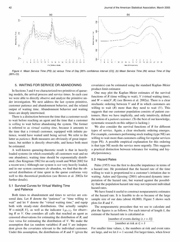