statistical analysis of momentum in basketball

Bowling Green State University Bowling Green State University

ScholarWorks@BGSU ScholarWorks@BGSU

Honors Projects Honors College

Winter 12-5-2017

Statistical Analysis of Momentum in Basketball Statistical Analysis of Momentum in Basketball

Mackenzi Stump [email protected]

Follow this and additional works at: https://scholarworks.bgsu.edu/honorsprojects

Part of the Analysis Commons, Applied Mathematics Commons, Applied Statistics Commons, Other

Computer Sciences Commons, Probability Commons, Statistical Methodology Commons, and the

Statistical Models Commons

Repository Citation Repository Citation Stump, Mackenzi, "Statistical Analysis of Momentum in Basketball" (2017). Honors Projects. 404. https://scholarworks.bgsu.edu/honorsprojects/404

This work is brought to you for free and open access by the Honors College at ScholarWorks@BGSU. It has been accepted for inclusion in Honors Projects by an authorized administrator of ScholarWorks@BGSU.

https://scholarworks.bgsu.edu/

https://scholarworks.bgsu.edu/honorsprojects

https://scholarworks.bgsu.edu/honors_college

https://scholarworks.bgsu.edu/honorsprojects?utm_source=scholarworks.bgsu.edu%2Fhonorsprojects%2F404&utm_medium=PDF&utm_campaign=PDFCoverPages

http://network.bepress.com/hgg/discipline/177?utm_source=scholarworks.bgsu.edu%2Fhonorsprojects%2F404&utm_medium=PDF&utm_campaign=PDFCoverPages








https://scholarworks.bgsu.edu/honorsprojects/404?utm_source=scholarworks.bgsu.edu%2Fhonorsprojects%2F404&utm_medium=PDF&utm_campaign=PDFCoverPages

STATISTICAL ANALYSIS OF MOMENTUM IN BASKETBALL

MACKENZI STUMP

HONORS PROJECT

Submitted to the Honors College

at Bowling Green State University in partial fulfillment of the

requirements for graduation with

UNIVERSITY HONORS 12/5/17

James Albert, Advisor

Dr. James Albert, Mathematics and Statistics

Christopher Rump, Advisor

Dr. Christopher Rump, Applied Statistics and Operations

Research

Abstract

The “hot hand” in sports has been debated for as long as sports have been around. The debate

involves whether streaks and slumps in sports are true phenomena or just simply perceptions in

the mind of the human viewer. This statistical analysis of momentum in basketball analyzes the

distribution of time between scoring events for the BGSU Women’s Basketball team from 2011-

2017. We discuss how the distribution of time between scoring events changes with normal

game factors such as location of the game, game outcome, and several other factors. If scoring

events during a game were always randomly distributed, or followed a specific model all of the

time, then streaks and slumps would simply be perceived phenomena during the game. This

study reveals that the scoring events within a game follow the Poisson process, and that the time

between scoring events for each game can typically be modeled by an exponential distribution

with a mean equal to the reciprocal of the average time between successive BGSU scoring events

within that game. However, even though the scoring events in most games are found to follow

the Poisson process, there are still a significant number of games in which the exponential model

does not fit the data well. These instances suggest that the particular game was unusually streaky,

either with larger gaps between scoring events occurring more often or smaller gaps between

scoring events occurring more often. These events indicate that the team was truly in a slump

and did not score very often, or was truly on a hot streak, suggesting that streaks and slumps are

more than just imagined events.

Index

I. Literature Review……………………………………………………………………………… 1

II. Introduction…………………………………………………………………………………… 3

III. Data Description………………………………………………………..……………………. 3

IV. Exploratory Analysis……………………………………………………………………….... 6

V. Modeling…………………………………………………………………………………….. 20

VI. Conclusion………………………………………………………………………………….. 26

VII. Honors Project Requirements……………………………………………………………… 28

VIII. References………………………………...………………………………………………. 31

IX. Appendices …………………………………………………………………………………. 32

1

I. Literature Review

It wasn’t until the 1970’s that sports analytics began making headway. In hopes of increasing the

likelihood of winning, baseball fanatics started to develop a range of statistical tools for

analyzing players, teams, and strategies. A perceived analytical advantage, as well as increased

computational power, and automated data collection methods sparked the growth of this field,

and now it’s expanding more than ever. Although sports analytics began in distinct event sports

such as baseball and tennis, it quickly transferred to more fluid sports such as basketball and

soccer. Professional teams nowadays spend several billions of dollars to hire experienced

performance analysts to analyze large quantities of data including play-by-play data, video

tracking data, and sensor readings (Van Haaren, 2016).

However, even as recent as 2015, coaches are still hesitant to fully rely on these analytics, and

spending so many resources on analytics is controversial as many coaches believe they know

what is best for their team and do not want the game to become too robotic. Nevertheless, it is

proven that several of the best ranked teams in basketball are the ones who have the most

sophisticated and high-tech analytic assets. This shift in analyzing player and team behavior has

forever changed the culture in which the game of basketball is viewed and played (Ross, 2015).

Nowadays, it is nearly impossible to talk about sports without a coach, player, or fan bringing up

the universal belief that momentum is an important force in sports contests. Evidence of this

perceived momentum can be found in the everyday lexicon of sports: hitting streaks and batting

slumps in baseball, the hot hand in basketball, or simply winning streaks in general. It has been

demonstrated that athletes, fans, and coaches alike all believe in the existence of momentum.

Other players pass to teammates that seem to be on a strong shooting streak, and coaches are

more likely to keep these streak players in the play longer based on perceived momentum

according to Vergin (2000). However, evidence for the effect of momentum on game

performance has been severely limited and controversial. How coaches and players should

respond to perceived momentum has been the question at hand for a while now: should coaches

and players go with their gut feelings and what they perceive, or rely on analytics to tell them

their next move?

As analytics continued to grow, the analysis of momentum in basketball began in 1985 with a set

of studies done by Gilovich, Vallone, and Tversky (1985). According to Michael Bar-Eli,

Simcha Avugos, and Markus Raab (2006), the term “hot hand,” or momentum, refers to the

“belief that successive attempts of an individual player are positively related, as well as the

behavior influenced by such a belief.” This can be interpreted as strong previous performance

leads to continued success in results whether that be for an individual player during a game or

team results across several games. Gilovich, Vallone, and Tversky (1985) found no evidence for

hot hand after studying the correlation between the outcomes of successive shots. Unfortunately,

only a few more studies since then have focused on momentum and its’ effects in basketball.

Most successive studies revolved around individual player momentum like Gilovich had done,

but used different methods of analysis, or focused more on creating sophisticated models to

predict the winner of a game (Bashuk, 2016), (Goldsberry, 2014), which is an entirely distinct

feat that involves several other factors in addition to momentum. Despite the variety of

approaches and methods of analysis including logistic regression analysis (LaRow, 2016), the

2

Wald-Wolfowitz test (Vergin, 2000), the Chi-Squared Goodness-of-Fit test (Vergin, 2000), self-

developed models (Arkes 2011), (LaRow, 2016), (Bocskocsky, Ezekowitz, Stein, 2014), and

SVM’s (LaRow, 2016), the mystery behind momentum in basketball remains uncertain.

Conclusions diverge about 50-50, suggesting the need for further analysis (Bar-Eli, 2006).

In a rapid turn of events, Trent McCotter (2010) determined that unlike many statisticians

believe, players’ games are not independent and identically distributed (IID) trials, further

upsetting the already controversial results of previous studies. For example, batters who are in

the midst of a hitting streak are more likely to continue the streak than one would expect by

chance. Players are aware of when they have hitting streaks and may try to extend their streak by

changing their behavior such as taking fewer walks or going for more singles than doubles.

Likewise, coaches may change the batting lineup so the players who have been hitting well

recently, most likely the players with streaks, will have more opportunities to hit, which changes

the likelihood of the streak continuing. This faulty assumption of IID underlies several former

studies, challenging the strength and validity of their conclusions. Further, this realization will

force future studies to approach the study of momentum and calculating probabilities of streaks

in sports quite differently.

Seeing the results of these studies as a fan, player, or coach might be a little unsettling. They

might think “how come we can see these streaks, but the data proves otherwise?” Well in 2012,

Gabel and Redner’s analysis found that the distribution of winning and losing streaks in sports

do arise from random statistical fluctuations. Their study indicated that a simple random-walk

model successfully captures many features of the observed scoring patterns in basketball, thus

the apparent streaks or slumps seen during a game are simply a consequence of a series of

random uncorrelated scoring events. Further, Gilovich, Vallone, and Tversky (1985) determined

the belief in hot hand and the apparent detection of streaks in random sequences of basketball

shooting statistics is attributed to a general misconception of chance in which even short random

sequences are thought to be highly representative of the overall shooting sample. Likewise,

memory bias of events contributes to fans, coaches, and players being more likely to remember a

sequence of a somewhat unlikely streak than a sequence in which a player rotates between

hitting and missing shots (Gilovich, Vallone, Tversky, 1985). As Tversky and Kahneman (1971)

wrote in “Belief in the Law of Small Numbers”, “subjects act as if every segment of the random

sequence must reflect the true proportion: if the sequence has strayed from the population

proportion, a corrective bias in the other direction is expected.” This notion is a misconception of

the fairness of the laws of chance and the law of small numbers. This fallacy is what allows for

players, fans, and coaches to “see” random sequences as streaks, yet most statistical analysis

proves otherwise.

Overall, there have been several attempts to measure momentum at the individual level and

within a single day’s performance, but there has been a lack of studies that focus on team

momentum within a game, or over a period of time. With the determination that all previous

studies have focused on individual player momentum, or individual sport momentum, Gayton,

Very, and Hearns (1993) decided to push momentum research in a new direction in 1993 by

studying the momentum of a team within an individual game of ice hockey. In this scenario,

momentum was defined to be either scoring the first goal or outscoring the opponent in the first

period of a game. The investigation determined that psychological momentum can be found in

3

team sports as both measures of momentum were found to be associated with an increased

probability of winning the game. This study can be transferred in design to examine momentum

in basketball as well. However, because basketball is much higher scoring game than ice hockey,

being one or a few points ahead of the other team at any given point in time may be less likely to

prove predictive of game outcome.

Because there has been a limited research on momentum, especially team momentum in

basketball, and previous studies have controversial conclusions, the mystery behind momentum

and its’ effects remain unsolved, and thus an excellent topic for further study.

II. Introduction

As a female athlete myself and with the lack of attention to women’s collegiate athletics in

statistical studies in sports, I chose to specifically focus my study on the Bowling Green State

University (BGSU) Women’s Basketball team. Pre-recorded play-by-play data for every game

over the past several seasons for this team is readily available and contains the desired

information for my analysis. This secondary data allows for the desired analysis to occur without

the tedious task of personally recording several years of data. My goal for this project is to

examine how team momentum varies by different game factors and to determine if the scoring

events of each game are random events that follow a particular exponential model.

The play-by-play data mentioned above will be used to determine the time between each scoring

event for every game over the past six seasons. Throughout this analysis, the time between

scoring events will serve as an indicator of momentum for BGSU’s basketball team. Successive

scoring events could occur very rapidly, may be very spread out with a lot of time between

events, or may fall somewhere in between these two extremes.

In section IV, the distribution of time between scoring events for each game will be analyzed

according to several variables, such as game location, outcome of the game, difficulty of

opponent, and more. This analysis will tell us what game variables correlate to longer or shorter

times between scoring events.

Section V will test if the distribution of scoring events for individual games can be modeled by

an exponential distribution with lambda equal to the reciprocal of the average time between

successive BGSU scoring events for that particular game.

III. Data Description

Before any analysis could begin, it was necessary to determine what data was going to be used

throughout the project, as well as prepare that data for exploration by means of scrapping,

cleaning, and organizing the data for ease of analysis.

The data to be used for this project has been previously collected and is available to view at

http://www.bgsufalcons.com/sports/2009/6/11/WBB_0611093840.aspx?path=wbball. The data

4

includes official full-game box scores, as well as quarterly box scores. In addition, play-by-play

data is available which depicts the time, score, and a description for each play of the game. This

play-by-play data will be used to look at how momentum, or scoring streaks and slumps, vary in

accordance with other game-related variables.

The original data provides the main information used in my analysis and is divided by quarter, or

halves when appropriate. There are several events during each game that are documented in the

play-by-play data including rebounds, missed shots, scoring events, assists, turnovers, fouls,

steals, blocked shots, substitutions, and timeouts. When either team scores, the number of

minutes and seconds left in the period is also recorded, along with the cumulative score for each

team at that point in time.

The first column is a description of the play for the BGSU Women’s Basketball team. The time

column indicates the amount of time remaining in the quarter or half; therefore, it starts at 10 or

20 minutes, respectively, and decreases thereafter. The third column indicates the updated scores

for each team. The fourth column indicates the margin: “H” means the home team is winning by

the stated number of points, “T” means the game is tied, and “V” indicates that the visiting team

is winning by the stated number of points. The last column specifies the type of game event for

the away team. A sample of the original play-by-play data from the BGSU Athletics website is

viewable in Appendix I.

The original data was read directly into R from the BGSU athletics website by using the

readLines function. Other data scrapping techniques were used to extract specific information

from the play-by-play data and organize this desired data into a data frame consisting of seven

variables: date, home team, visiting team, minutes remaining in the period, seconds remaining

in the period, cumulative home score, and cumulative visitor score.

This read and extract process was repeated for 188 games that were played over the course of

the past six seasons, resulting in over 12,000 lines of data that indicated one scoring event per

row. This initial information collected from the secondary source served as the base from which

all other information needed for the analysis could be derived.

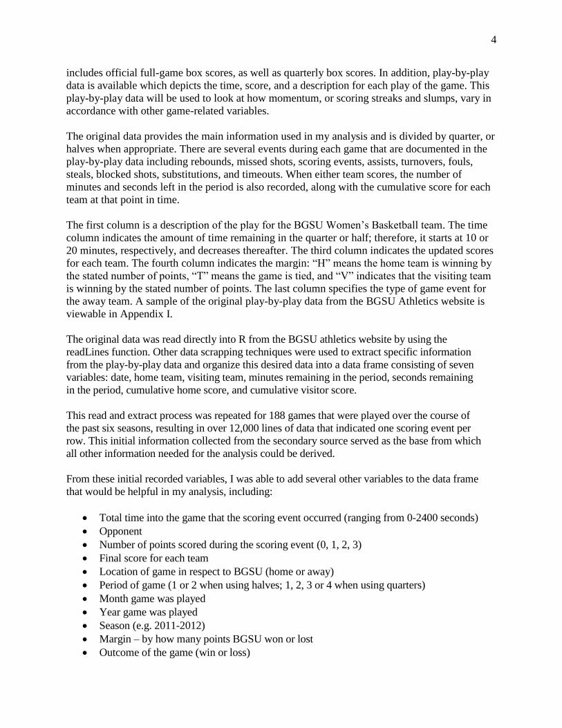
From these initial recorded variables, I was able to add several other variables to the data frame

that would be helpful in my analysis, including:

• Total time into the game that the scoring event occurred (ranging from 0-2400 seconds)

• Opponent

• Number of points scored during the scoring event (0, 1, 2, 3)

• Final score for each team

• Location of game in respect to BGSU (home or away)

• Period of game (1 or 2 when using halves; 1, 2, 3 or 4 when using quarters)

• Month game was played

• Year game was played

• Season (e.g. 2011-2012)

• Margin – by how many points BGSU won or lost

• Outcome of the game (win or loss)

5

• Time between each scoring event

• Time between each of BGSU’s scoring events

• Total number of scoring events for both teams during the game

• Total number of scoring events for BGSU during the game

• Total points scored by both teams during the game

A few other variables were also added to the data frame after individual collection. I created a

spreadsheet in Excel that incorporated the following information for each team:

• League

• 2016-2017 NCAA RPI

• W-L record for each season

The Mid-American Conference (MAC) ranking for the BGSU Women’s Basketball team was

also collected for all six seasons. These separate spreadsheets were also read into R and

combined with the main data frame for further analysis. These additional variables became

useful when analyzing how the time between scoring events for the BGSU Women’s

Basketball team differed by difficulty of opponent, league of opponent, and ranking in the

MAC league.

Lastly, two more variables were created in order to analyze whether the scoring events in each

individual game followed an exponential distribution with a mean related to the number of

scoring events by BGSU’s Women’s Basketball team.

• P-value – p-value calculated from a chi-square goodness-of-fit test that provides the

probability that the scoring events within a given game follow the exponential

distribution with a mean related to the number of scoring events by BGSU

• Significance – yes/no response to whether the p-value mentioned above is significant

After all of these variables were combined into one data frame, a second data frame was then

created to incorporate only those scoring events that were unique to BGSU’s team. Therefore,

every line of data in this data frame represented one scoring event for the BGSU Women’s

Basketball team. This step was vital in allowing us to focus solely on scoring events by BGSU.

The time between scoring events was then updated to reflect the time between successive

BGSU scoring events, rather than the time between the current scoring event and previous

scoring event regardless of team. It is important to distinguish these particular scoring events of

interest, otherwise we would be analyzing the time between scoring events between both teams,

which would not reflect the scoring distribution of the individual team of interest.

Each of the variables collected or created during the initial stages of the project will be further

analyzed in the next section by using summary statistics and through graphical relationships

between several of the variables. This exploratory analysis will help us understand the

distribution of scoring events during games and how this distribution changes based on other

game-related factors.

6

IV. Exploratory Analysis

A. Distribution of Time between Scoring Events

First we begin with the analysis of some basic descriptive statistics to better understand what the

data looks like. The distribution of time between successive scoring events for the BGSU

Women's Basketball team over the past six year is described below.

During some basic exploratory analysis, I uncovered that there were several scoring events that

occurred simultaneously or had zero seconds between each scoring event. I chose to remove

cases in which the time between scoring events was 0 seconds because these instances occurred

when there was more than one successive free throw. It is important to incorporate the first free

throw in a set of consecutive free throws in the analysis as it does represent a scoring event;

however, successive free throws are not considered separate scoring events in this analysis and

will be excluded from the study.

There was also a small subset of four games in which both teams were tied at the end of

regulation. These games then continued into an overtime period of five minutes. Since the

distribution of scoring events during these games may be systematically different than games

that do not go into overtime, and because the sample size is so small, I chose to exclude these

four games from the analysis as well.

Overall, there were a total of 184 games played over a six year period included in this analysis.

There were 12,262 scoring events for all teams, and a subset of 6,331 scoring events for BGSU's

team alone, 994 of which were free throws that were removed from the dataset. In the analysis

below, I focused specifically on the wait times between successive scoring events in relation to

BGSU's team only. Therefore, the time between scoring events refers to the time it took BGSU

to score again from their previous scoring event.

The minimum time between two successive scoring events was 0 seconds, and this event would

be attributed to a free throw shot. Excluding free throws, the minimum time between successive

scoring events was 1 second. The maximum time between successive scoring events by BGSU

was 569 seconds, or 9 minutes and 29 seconds. This would be considered a very large scoring

drought in the sport of basketball, and would be very rare for a drought of this magnitude to

occur. 25% of scoring events occurred within 37 seconds of the previous scoring event for

BGSU. 50% occurred within 61 seconds, and 75% occurred within 105 seconds.

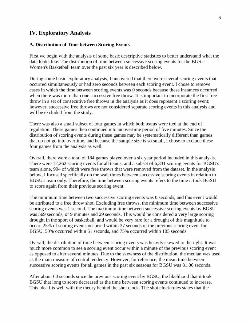
Overall, the distribution of time between scoring events was heavily skewed to the right. It was

much more common to see a scoring event occur within a minute of the previous scoring event

as opposed to after several minutes. Due to the skewness of the distribution, the median was used

as the main measure of central tendency. However, for reference, the mean time between

successive scoring events for all games in the past six seasons for BGSU was 81.06 seconds.

After about 60 seconds since the previous scoring event by BGSU, the likelihood that it took

BGSU that long to score decreased as the time between scoring events continued to increase.

This idea fits well with the theory behind the shot clock. The shot clock rules states that the

7

offensive team must attempt a field goal with the ball leaving the player's hand before the shot

clock expires, and the shot must either touch the rim or enter the basket. The implementation of

the shot clock serves the purpose of increasing the pace of the game and creating more scoring

events. Since the team in possession must attempt a shot within 30 seconds of gaining

possession, it seems fitting that 50% of scoring events are made within 61 seconds, slightly

longer than double the shot clock value. This would give enough time for the opposing team to

have a full possession, as well as allow BGSU to have one full possession before scoring again.

This is obviously not the case for all scoring events, as each possession results in different

outcomes, however, it merely indicates that the distribution of time between scoring events fits in

as expected with the rules of the game.

Figure 1: The distribution of time between BGSU’s scoring events are graphed in the

boxplot above. The distribution is heavily skewed towards smaller values with the

majority of scoring events occurring within 200 seconds of the previous scoring event.

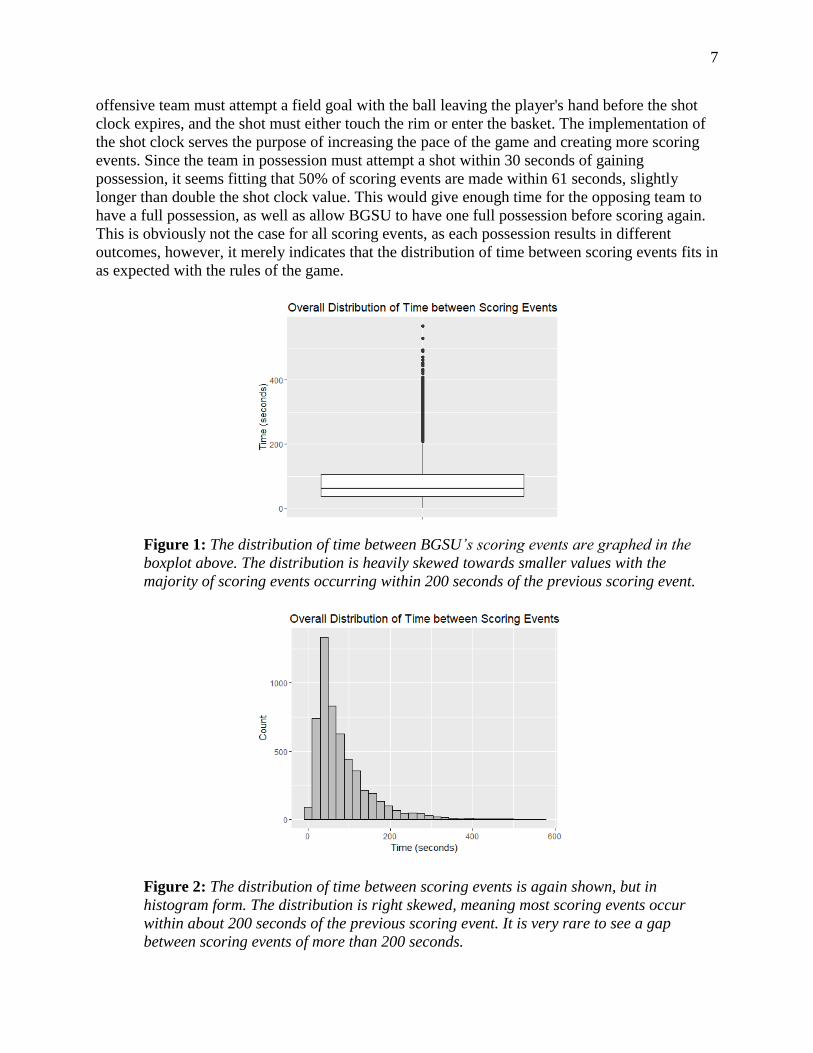
Figure 2: The distribution of time between scoring events is again shown, but in

histogram form. The distribution is right skewed, meaning most scoring events occur

within about 200 seconds of the previous scoring event. It is very rare to see a gap

between scoring events of more than 200 seconds.

8

B. Period

Before the 2015-2016 season started, the NCAA introduced a new rule to women's college

basketball: the game was now to be played using quarters rather than halves. Consequently, I

chose to split my data into each respective group with older seasons being analyzed by half and

more recent seasons being analyzed by quarter to be consistent with this change.

In my data, seasons 2011-2012, 2012-2013, 2013-2014, and 2014-2015 were played using

halves. Looking at the Figure 3, there is a very small difference in times between scoring events

for each half. 50% of scoring events occurred with 61 seconds of the previous event for the first

half of the game and within 58 seconds of the second half of the game. There were 1,787 scoring

events in the first half of all 129 games in the first four seasons, averaging to 13.85 scoring

events per first half, and there were 2,024 scoring events in the second half of all 129 games,

averaging 15.69 scoring events per second half. This data suggests that on average, BGSU

increased up the pace of their scoring in the second half of each game.

Seasons 2015-2016 and 2016-2017 were played using quarters. The fourth quarters had the

lowest median wait time between scoring events at 55 seconds, while the second quarters had

longest median wait time between scoring events at 69.5 seconds. It is not surprising that the

fourth quarters exhibit lower quartiles for times between successive scoring events as in most

games in sports, teams usually pick up their intensity towards the end of the game to either

ensure a win, or try to catch up to their opponent if losing. Picking up the intensity would result

in an average of more scoring events and less time between those scoring events.

Figure 3: Displayed above is a set of boxplots depicting the time between scoring events

by quarter. This graph only represents the data from seasons 2015-2016 and 2016-2017

as previous seasons were played using halves. There are very small differences among

each group. Quarter 2 seems to have slightly larger wait times between scoring events

while on average, Quarter 4 has slightly less wait times between scoring events.

9

Figure 4: The distribution of time between scoring events by half is displayed above. This

graph only represents data from seasons prior to the 2015-2016 season, as more recent

seasons are played using quarters. There is a very small difference among each group.

The first half has a slightly larger interquartile range and slightly larger median in

regards to the time between scoring events as compared to the second half of the games.

C. Location

It is often argued that the home team has the advantage of playing on their own court, and so this

comfort of familiarity and lack of travel should increase the home team’s chances of winning. If

this is true, and the home team wins more often, we would likely see that the home team scores

more often and has smaller gaps between scoring events.

Figure 5: The pair of boxplots above depict the time between scoring events by location:

home or away. Home games have a significantly smaller interquartile range and lower

median in regards to the wait times between scoring events.

10

There were 88 away games and 96 home games played by BGSU. 50% of points were scored

within 58 seconds of the previous scoring event for home games, while 50% of points were

scored within 63 seconds of the previous scoring event for away games. 59.57% of away games

were won, while 68.7% of home games were won. There were also 2,397 scoring events in the

88 away games, averaging 27.24 scoring events per game, while there were 2,940 scoring events

in the 96 home games, averaging 30.625 scoring events per game. These numbers clearly

indicate a trend that, on average, the time between scoring events was larger for away games

than for home games, and thus, because the home team was scoring more often, they scored

more points during the game and were more likely to win the game as opposed to away games.

D. Difficulty of Opponent

At this point, I thought it would be interesting to see how the time between scoring events varied

according to the difficulty of the opponent. The difficulty of the opponent was measured by the

NCAA RPI ranking. This ranking variable was only available for the 2016-2017 season, thus

only the times between scoring events for that season were included in this particular analysis.

From Figures 6 and 7, the three graphs depict that there are no identifiable trends that detect how

the times between scoring events differ based on opponent difficulty. The times between scoring

events vary greatly and randomly as RPI ranking increases.

Figure 6: Both graphs above represent the wait times between scoring events based on

the 2016-2017 NCAA RPI ranking of each opponent BGSU played during the 2016-2017

season. The leftmost side of each graph represents teams with a low RPI, meaning they

are ranked higher according to the NCAA. The right hand side of each graph represents

teams with higher RPI rankings meaning they are ranked lower according to the NCAA.

A rank of 0 indicates that the given opponent was unranked in the NCAA. There is no

conclusive relationship between NCAA RPI Ranking and the distribution of time between

scoring events.

11

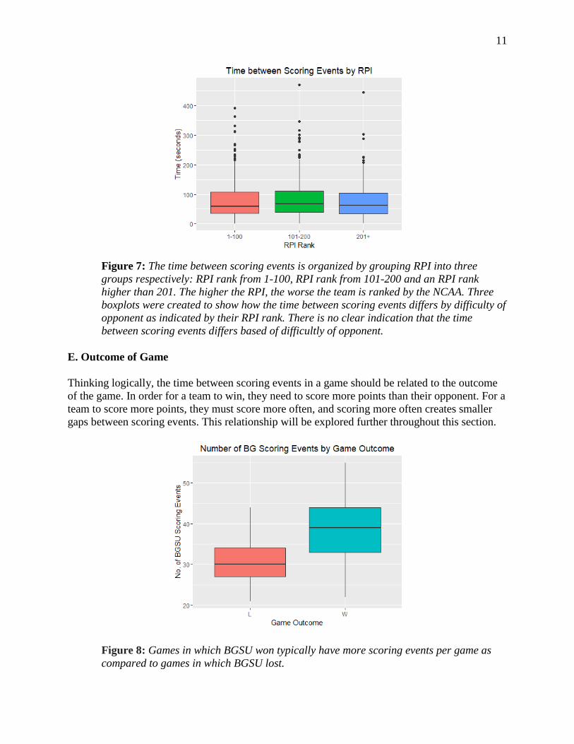
Figure 7: The time between scoring events is organized by grouping RPI into three

groups respectively: RPI rank from 1-100, RPI rank from 101-200 and an RPI rank

higher than 201. The higher the RPI, the worse the team is ranked by the NCAA. Three

boxplots were created to show how the time between scoring events differs by difficulty of

opponent as indicated by their RPI rank. There is no clear indication that the time

between scoring events differs based of difficultly of opponent.

E. Outcome of Game

Thinking logically, the time between scoring events in a game should be related to the outcome

of the game. In order for a team to win, they need to score more points than their opponent. For a

team to score more points, they must score more often, and scoring more often creates smaller

gaps between scoring events. This relationship will be explored further throughout this section.

Figure 8: Games in which BGSU won typically have more scoring events per game as

compared to games in which BGSU lost.

12

In games that BGSU won, BGSU scored within 56 seconds of their previous scoring event 50%

of the time. In comparison, in games that BGSU lost, BGSU scored within 68 seconds of their

previous scoring event 50% of the time. BGSU won 109 games over the six year study period,

and lost 75 games. There were 3,419 scoring events in the 109 games they won and only 1,918

scoring events in the 75 games they lost. This succumbed to an average of 31.37 scoring events

per game in games that BGSU won and an average of only 25.57 scoring events per game in

games that BGSU lost. These statistics work together to show that, on average, games in which

BGSU won had lower wait times between scoring events than in games they lost. This is to be

expected since in order to win a game, the team would need to score more often, thus creating

less time between successive scoring events.

Figure 9: The boxplots above depict the time between scoring events by game outcome:

win or loss. Games that BGSU won have a significantly smaller interquartile range and

lower median in regards to the wait times between scoring events.

F. Margin

The margin score indicates how many points BGSU's Women's Basketball team won or lost by

in a given game. A positive margin score, such as 15, reflects a win for BGSU by 15 points. A

negative margin score, such as -15, reflects a loss for BGSU by 15 points. The distribution of

margin scores was fairly symmetrical. Over all six seasons, the margin ranged from an extreme

loss by 47 points to an extreme win by 50 points. 50% of all games were won by a margin of at

least 6 points. The margin can never be 0 points as ties are not allowed and will move into

overtime periods. Overtime games were eliminated from this analysis for simplicity and potential

systematic differences between normal games and those games that go into overtime.

13

Figure 10: The left graph is a boxplot representing the game margin distribution of all

games BGSU Women’s basketball played over the past 6 seasons. A positive margin

indicates a win for BGSU by the stated number of points, and a negative margin indicates

a loss for BGSU by the stated number of points. There cannot be a margin score of zero

as any tied game immediately moves into overtime. The distribution of margin is fairly

symmetric about the median of six points.

From first glance at Figure 11, it is hard to tell if there is a significant difference in times

between scoring events by margin. Looking closely at the upper outliers may indicate a slight

negative trend as margin increased, the wait times between scoring events decreased. However,

this is very difficult to tell in the mass of data points in the graph.

Figure 11: Distribution of wait times between scoring events by game margin is shown

above. As margin increases, the overall range of times between scoring events decreases.

The red circled area was added to highlight the negative trend of the upper outliers.

Po

ints

14

Figure 12 organizes the wait times between scoring events by grouping margin into four groups:

a margin of -50 to -25, indicating a very bad loss, a margin of -25 to 0, indicating a minor loss, 0-

25, indicating a minor win, and 25-50, indicating a very good win. Grouping margin in this way

created a much better visual that depicts how the wait times between scoring events typically

decreased as BGSU won by more points, or lost by less points. As margin increased, the

interquartile range of wait times between scoring events decreased, as did the median for each

group. This corresponds to the findings outlined in Section E. When the team wins, or even wins

by more points, the time between scoring events typically decreases. This is to be expected as a

winning team must score more often, resulting in less time in between successive scoring events.

Figure 12: Time between scoring events by margin is depicted, but this time, the margin

of the games has been divided into four groups. The leftmost group indicates extreme

losses, while the rightmost group represents extreme wins. As margin increases relative

to BGSU, the interquartile range of time between scoring events decreases, as do the

total range and median of each group.

G. Season

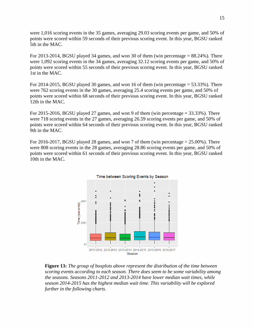
The boxplots in Figure 13 suggest that there is not a huge difference in time between successive

scoring events by season; however, when you look closer into the data, there is a relationship

between the time between scoring events, the average number of scoring events per game,

BGSU’s overall MAC ranking for that year, and BGSU’s win percentage for the season.

For 2011-2012, BGSU played 30 games, and won 23 of them (win percentage = 76.67%). There

were 941 scoring events in the 30 games, averaging 31.37 scoring events per game, and 50% of

points were scored within 57 seconds of their previous scoring event. In this year, BGSU ranked

2nd in the MAC.


15

were 1,016 scoring events in the 35 games, averaging 29.03 scoring events per game, and 50% of


5th in the MAC.


were 1,092 scoring events in the 34 games, averaging 32.12 scoring events per game, and 50% of


1st in the MAC.




12th in the MAC.




9th in the MAC.




10th in the MAC.

Figure 13: The group of boxplots above represent the distribution of the time between

scoring events according to each season. There does seem to be some variability among

the seasons. Seasons 2011-2012 and 2013-2014 have lower median wait times, while

season 2014-2015 has the highest median wait time. This variability will be explored

further in the following charts.

16

Figure 14: This graph describes how the total number of scoring events per season

differed by BGSU’s rank within the MAC league for the given season. The leftmost point

indicates that in the 2013-2014 season, the total number of scoring events for the season

was around 1,100 events, and BGSU was ranked 1st in the MAC League. The rightmost

point on the graph indicates that in the 2014-2015 season, BGSU was ranked 12th and

had only 760 scoring events in the whole season. As BGSU’s rank in the MAC league

decreased, the number of scoring events per season also typically decreased.

In the first three seasons analyzed above (2011-2012, 2012-2013, and 2013-2014), there appears

to be a lower wait time between successive scoring events which led to an average of more

scoring events per game, more wins per season, and thus, a higher overall ranking in the MAC

for the given season.

H. Month

Out of the 184 games being analyzed, 33 games were played in November, 35 in December, 46

in January, 43 in February, and 27 in March. BGSU won 19 out of the 33 games in November,

creating a 57.58% win percentage, 21 out of the 35 games in December, creating a 60.00% win

percentage, 30 out of the 46 games in January, creating a 65.22% win percentage, 27 out of the

43 games in February, creating a 62.79% win percentage, and only 12 out of the 27 games in

March, creating a win percentage of only 44.44%. BGSU's most successful month was clearly

January, while their least successful month was March. BGSU had 1,302 scoring events in

January and 774 scoring events in March. This computed to an average of 28.3 scoring events

per game in January and an average of 28.67 scoring events per game in March. This is

surprising as we would expect a month with a higher average win percentage to typically have

more scoring events per game as more scoring events lead to more points and a higher chance of

winning. It is strange to see that both months have a similar average number of scoring events

per game. This would suggest perhaps that the opponents played in March also had less scoring

events, and were overall, lower scoring games.

17

There is not a large difference in the times between scoring events by month. 50% of scoring

events occurred between 55 to 62 seconds of the previous event for all months. There does not

seem to be a relationship between average times between scoring events and win percentage by

month.

Figure 15: The light blue indicates the total number of games played each month over

the past six seasons. The most games are played in January and February while the least

amount of games are played in March. The dark blue inset represents the total number of

games won each month over the past six seasons. The white text in the dark blue column

indicates the percent of games won each month. January had the highest percentage of

wins, while March had the lowest percentage of wins

Figure 16: These boxplots represent the wait times between scoring events by month.

There is not a major distinction between each group, concluding that BGSU’s score

distribution is fairly consistent each month.

Games Played

Games Won

44.44%

62.79%65.22%

60.00%57.58%

18

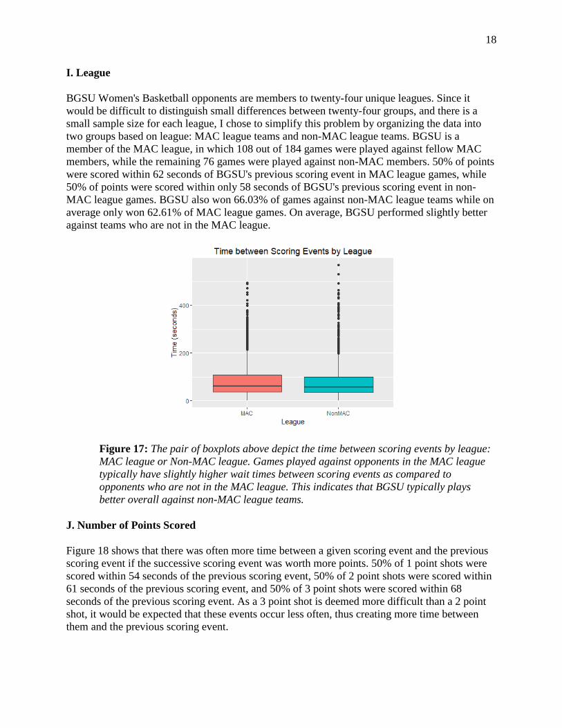
I. League

BGSU Women's Basketball opponents are members to twenty-four unique leagues. Since it

would be difficult to distinguish small differences between twenty-four groups, and there is a

small sample size for each league, I chose to simplify this problem by organizing the data into

two groups based on league: MAC league teams and non-MAC league teams. BGSU is a

member of the MAC league, in which 108 out of 184 games were played against fellow MAC

members, while the remaining 76 games were played against non-MAC members. 50% of points

were scored within 62 seconds of BGSU's previous scoring event in MAC league games, while

50% of points were scored within only 58 seconds of BGSU's previous scoring event in non-

MAC league games. BGSU also won 66.03% of games against non-MAC league teams while on

average only won 62.61% of MAC league games. On average, BGSU performed slightly better

against teams who are not in the MAC league.

Figure 17: The pair of boxplots above depict the time between scoring events by league:

MAC league or Non-MAC league. Games played against opponents in the MAC league

typically have slightly higher wait times between scoring events as compared to

opponents who are not in the MAC league. This indicates that BGSU typically plays

better overall against non-MAC league teams.

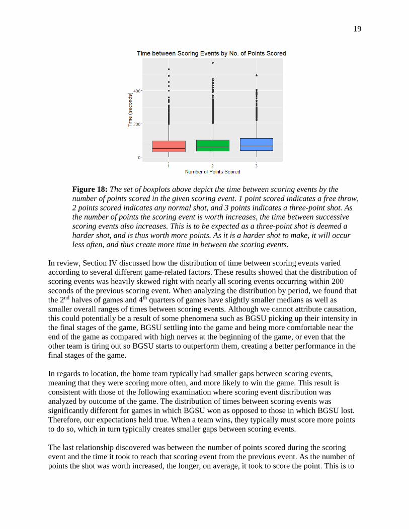
J. Number of Points Scored

Figure 18 shows that there was often more time between a given scoring event and the previous

scoring event if the successive scoring event was worth more points. 50% of 1 point shots were

scored within 54 seconds of the previous scoring event, 50% of 2 point shots were scored within

61 seconds of the previous scoring event, and 50% of 3 point shots were scored within 68

seconds of the previous scoring event. As a 3 point shot is deemed more difficult than a 2 point

shot, it would be expected that these events occur less often, thus creating more time between

them and the previous scoring event.

19

Figure 18: The set of boxplots above depict the time between scoring events by the

number of points scored in the given scoring event. 1 point scored indicates a free throw,

2 points scored indicates any normal shot, and 3 points indicates a three-point shot. As

the number of points the scoring event is worth increases, the time between successive

scoring events also increases. This is to be expected as a three-point shot is deemed a

harder shot, and is thus worth more points. As it is a harder shot to make, it will occur

less often, and thus create more time in between the scoring events.

In review, Section IV discussed how the distribution of time between scoring events varied

according to several different game-related factors. These results showed that the distribution of

scoring events was heavily skewed right with nearly all scoring events occurring within 200

seconds of the previous scoring event. When analyzing the distribution by period, we found that

the 2nd halves of games and 4th quarters of games have slightly smaller medians as well as

smaller overall ranges of times between scoring events. Although we cannot attribute causation,

this could potentially be a result of some phenomena such as BGSU picking up their intensity in

the final stages of the game, BGSU settling into the game and being more comfortable near the

end of the game as compared with high nerves at the beginning of the game, or even that the

other team is tiring out so BGSU starts to outperform them, creating a better performance in the

final stages of the game.

In regards to location, the home team typically had smaller gaps between scoring events,

meaning that they were scoring more often, and more likely to win the game. This result is

consistent with those of the following examination where scoring event distribution was

analyzed by outcome of the game. The distribution of times between scoring events was

significantly different for games in which BGSU won as opposed to those in which BGSU lost.

Therefore, our expectations held true. When a team wins, they typically must score more points

to do so, which in turn typically creates smaller gaps between scoring events.

The last relationship discovered was between the number of points scored during the scoring

event and the time it took to reach that scoring event from the previous event. As the number of

points the shot was worth increased, the longer, on average, it took to score the point. This is to

20

be expected as a shot worth more points is deemed more difficult and is less likely to occur, and

when this event occurs less often, the time between these events will increase.

Conversely, there were two factors that seemed to have little to no correlation with the

distribution of scoring events. There was no clear indication that the time between scoring events

had any correlation with the difficulty of opponent. This is surprising as one might naturally

expect the team to score less points against harder teams, creating larger gaps between scoring

events. However, this is not the case. Additionally, there was no major distinction between the

distributions of scoring events for games played against opponents who were in the MAC league

versus in those games that were played against teams not in the MAC league. This indicates that

BGSU competed fairly consistently in both league and non-league games.

Overall, we see that several game-related factors are correlated with the times between scoring

events just as we would expect, while others are not. This exploratory analysis was used to gain a

deeper understanding of the relationships between momentum and these game-related factors.

However, the initial exploratory analysis provided no further progress to whether the “hot hand”

exists, or that scoring events are independent random events. Section V of this paper will analyze

the distribution of scoring events further by determining whether scoring events are truly random

and follow the Poisson process.

V. Modeling

A. Poisson Process

The Poisson distribution has been used to calculate the probability of an independent event

occurring based on the mean number of successes dating back to 1898 when Ladislaus

Bortkiewicz modeled the number of deaths by horse kick in Prussia cavalry (Pandian, Kumar,

2015).

A Poisson process is a probability model for describing the occurrence of events in time. Let

N(t) denote the number of events that occur in the time interval from 0 to t. A Poisson process

assumes that the number of events at time 0 is 0, that is, N(0) = 0. In addition, the number of

events observed in an interval of length t only depends on the value of t, not when the

observation begins. Lastly, the number of observations in an interval of length t is given by a

Poisson distribution with mean lambda t, where the rate per unit time is equal to lambda.

One implication of a Poisson process model is that the spacings between successive individual

outcomes are exponentially distributed with a rate of occurrence equal to lambda (λ). The

exponential distribution deals with the time between each of these occurrences of successive

events as time flows by continuously (Kerns, 2010).

The exponential distribution is unique due to its “lack-of-memory” property. This means that the

chance of success at any given time is equal to the reciprocal of the mean success rate:

λ = 1

𝑚𝑒𝑎𝑛 𝑠𝑢𝑐𝑐𝑒𝑠𝑠 𝑟𝑎𝑡𝑒

21

For example, after waiting for one minute without a phone call, the probability of a call arriving

in the next two minutes is the same as the probability of getting a phone call in the two minutes

following a call. Therefore, as you continue to wait, the chance of something happening “soon”

neither increases nor decreases (Kerns, 2010). Other real life examples of the Poisson process are

the number of visitors to a web site per minute, the number of hungry people entering Chipotle

per day, the number of arrivals at a car wash in one hour, and the number of bankruptcies that are

filed in a month. As you can see, it is not uncommon for what seems like random occurrences to

follow this Poisson process.

In the case of basketball, if we assume that scoring events are truly random, independent events,

and that streaks and slumps are merely perceptions of the human eye, then in theory, we should

be able to model the scoring events within each game using the Poisson distribution with the

mean number of successes equal to the average number of scoring events by BGSU for that

game.

Randomly simulated data below provides an example of what an exponential distribution may

look like. For example, look at the graph in Figure 19. Suppose this data represents the

distribution of time between scoring events for one game. During this game, the average time

between scoring events is 20 seconds, which is equivalent to averaging three scoring events per

minute. Therefore, there are some scoring events that happen sooner than every 20 seconds, and

some that occur after that 20 seconds has passed. We can also see that it is very unlikely that a

scoring event would occur 80 seconds after the previous scoring event given a mean scoring rate

of 20 seconds.

Figure 19: This graph represents data that follows an exponential model with an average

scoring rate of 1 scoring event per 20 seconds (λ=1/20), or three scoring events per

minute. This example shows what the data for time between scoring events would look

like if it perfectly followed an exponential distribution with 𝑦 = 𝜆𝑒−𝜆𝑥, λ=1/20.

Exponentially distributed data fits along the exponential curve very well. Data that does

not follow this exponential curve well indicates that the scoring events are not

exponentially distributed. Keep this example in mind when comparing exponential

models with the distributions of the real data in Figure 20.

𝜆𝑒−𝜆𝑥

22

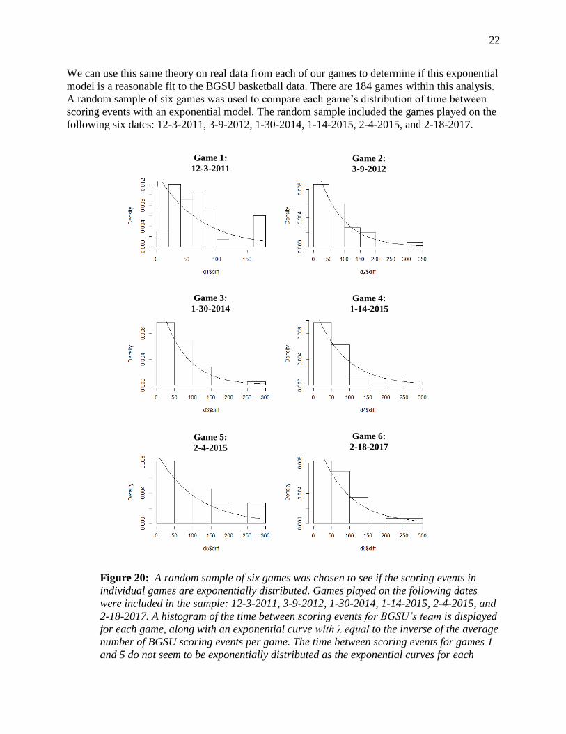
We can use this same theory on real data from each of our games to determine if this exponential

model is a reasonable fit to the BGSU basketball data. There are 184 games within this analysis.

A random sample of six games was used to compare each game’s distribution of time between

scoring events with an exponential model. The random sample included the games played on the

following six dates: 12-3-2011, 3-9-2012, 1-30-2014, 1-14-2015, 2-4-2015, and 2-18-2017.

Figure 20: A random sample of six games was chosen to see if the scoring events in

individual games are exponentially distributed. Games played on the following dates

were included in the sample: 12-3-2011, 3-9-2012, 1-30-2014, 1-14-2015, 2-4-2015, and

2-18-2017. A histogram of the time between scoring events for BGSU’s team is displayed

for each game, along with an exponential curve with λ equal to the inverse of the average

number of BGSU scoring events per game. The time between scoring events for games 1

and 5 do not seem to be exponentially distributed as the exponential curves for each

Game 1:

12-3-2011 Game 2:

3-9-2012

Game 3:

1-30-2014

Game 6:

2-18-2017 Game 5:

2-4-2015

Game 4:

1-14-2015

23

game do not fit the data well. However, for games 2, 3, 4 and 6, the exponential curves

do fit the data well, providing evidence that the BGSU scoring events may be

exponentially distributed throughout each game.

Looking at Figure 30, we see six histograms of the times between scoring events for BGSU for

each game in the sample, along with an exponential curve related to the total number of BGSU

scoring events per game. The time between scoring events for games 1 and 5 do not seem to be

exponentially distributed as the exponential curves for each game do not fit the data well.

However, for games 2, 3, 4 and 6, the exponential curves do fit the data well, providing evidence

that the BGSU scoring events may be exponentially distributed throughout each game.

B. Chi-Square Goodness-of-Fit Test

The next step in this analysis to determine if the scoring events for individual games follow an

exponential distribution was to perform the chi-square goodness-of-fit test. This statistical test

would help identify if we have evidence that suggests BGSU’s scoring events are consistent with

the specified exponential distribution, or that the scoring events do not follow an exponential

distribution. The null and alternative hypotheses for the goodness-of-fit test are stated below:

Null Hypothesis: Times between scoring events follow the exponential model:

𝑦 = 𝜆𝑒−𝜆𝑥, λ= 1

𝑚𝑒𝑎𝑛 𝑡𝑖𝑚𝑒 𝑏𝑒𝑡𝑤𝑒𝑒𝑛 𝑠𝑐𝑜𝑟𝑖𝑛𝑔 𝑒𝑣𝑒𝑛𝑡𝑠

Alternative Hypothesis: Times between scoring events do not follow the exponential model:

𝑦 = 𝜆𝑒−𝜆𝑥, λ= 1

𝑚𝑒𝑎𝑛 𝑡𝑖𝑚𝑒 𝑏𝑒𝑡𝑤𝑒𝑒𝑛 𝑠𝑐𝑜𝑟𝑖𝑛𝑔 𝑒𝑣𝑒𝑛𝑡𝑠

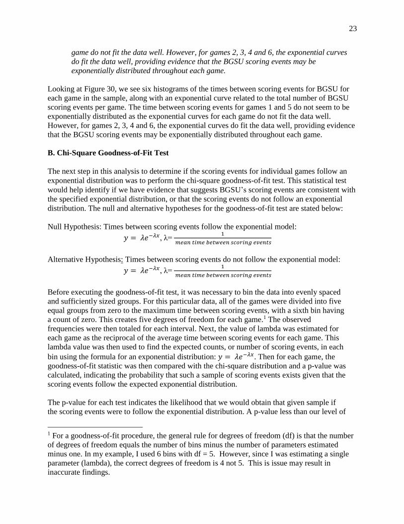
Before executing the goodness-of-fit test, it was necessary to bin the data into evenly spaced

and sufficiently sized groups. For this particular data, all of the games were divided into five

equal groups from zero to the maximum time between scoring events, with a sixth bin having

a count of zero. This creates five degrees of freedom for each game.1 The observed

frequencies were then totaled for each interval. Next, the value of lambda was estimated for

each game as the reciprocal of the average time between scoring events for each game. This

lambda value was then used to find the expected counts, or number of scoring events, in each

bin using the formula for an exponential distribution: 𝑦 = 𝜆𝑒−𝜆𝑥. Then for each game, the

goodness-of-fit statistic was then compared with the chi-square distribution and a p-value was

calculated, indicating the probability that such a sample of scoring events exists given that the

scoring events follow the expected exponential distribution.

The p-value for each test indicates the likelihood that we would obtain that given sample if

the scoring events were to follow the exponential distribution. A p-value less than our level of

1 For a goodness-of-fit procedure, the general rule for degrees of freedom (df) is that the number

of degrees of freedom equals the number of bins minus the number of parameters estimated

minus one. In my example, I used 6 bins with df = 5. However, since I was estimating a single

parameter (lambda), the correct degrees of freedom is 4 not 5. This is issue may result in

inaccurate findings.

24

significance of alpha=0.05 means that the probability that the scoring events would occur as

they did would be less than 5% if the scoring events truly followed the Poisson process. When

the p-value is less than 0.05, we reject the null hypothesis. In this case, we have evidence to

conclude that the data are consistent with the exponential distribution. If we obtain a p-value

greater than 0.05, we fail to reject the null hypothesis with 95% confidence. In this case, we

have evidence that the scoring events are not modeled by the exponential distribution well.

The Chi-squared test statistic, degrees of freedom and p-value for each game of the random

sample of six games is displayed in the chart below. Significant p-values at the 0.05 level of

significance are starred.

Game X-squared Degrees of Freedom P-value

1 15.2442 5 0.009368***

2 1.202 5 0.9447

3 4.2871 5 0.5089

4 4.565 5 0.4712

5 7.9199 5 0.1607

6 3.6833 5 0.5959

Figure 21: The chi-squared test statistic, degrees of freedom and p-value for each

game of the random sample of six games is displayed in the chart above. Significant

p-values at the 0.05 level of significance are starred. For game 1, we reject the null

hypothesis. We have evidence that suggests the scoring events for that game do not

follow the exponential model. However, in games 2-6, the p-value is greater than 0.05,

so we fail to reject the null hypothesis. We do not have evidence to conclude that the

scoring events for each of these five games do not follow the exponential model.

The chi-squared goodness-of-fit test showed us that five out of the six randomly selected

games did not have significant p-values, and thus, we failed to reject the null hypothesis for

these five out of six games. We did not have evidence to conclude that the scoring events do

not follow an exponential model. This sample provided reason to further test the theory that

scoring events within a game of basketball follow the Poisson process on the remaining

games in our data.

Next, the goodness-of-fit test was performed on all games. In doing so, we found that 156 out

of 184 games, or 84.78% of games, had a p-value greater than 0.05, meaning we had no

evidence that the scoring events within those games do not follow the exponential

distribution. Only 28 out of the 184 games had a significant p-value less than 0.05. This

means that 15.22% of games have evidence that the scoring events within those games do not

follow the exponential distribution.

25

Figure 22: The chi-squared goodness-of-fit test was performed on all 184 games. The

distribution of p-values for this test is shown above. A p-value less than 0.05 indicates

that we have evidence that the scoring events in the given game are not exponentially

distributed with a mean proportional to the reciprocal of the average time between

scoring events during that game. The distribution is bimodal. There is a peak near the

p-value of zero, indicating that the scoring events for each game are very unlikely to

follow the Poisson process. The second peak occurs around a p-value of 0.65. These

games provide no evidence that the scoring events do not follow the exponential

distribution.

Overall, we can conclude that in most games, scoring events typically follow an exponential

distribution with a lambda equal to the reciprocal of the average time between scoring events

for that particular game. We can see that most scoring events occurred fairly quickly after the

previous scoring event, and it is much less likely to see larger gaps between scoring events

during a game.

Games in which the distribution of times between scoring events did not follow an

exponential distribution, such as in game 1 of the random sample in Figure 20, indicate that

the team is being unusually streaky in their play, meaning there were larger gaps in between

scoring events, and that these gaps were more common. This is exactly the type of slumps that

coaches want to avoid as longer gaps between scoring events lead to less scoring events.

Generally, we can see that the scoring events in most games were random events that follow

the Poisson process; however, there were games that did not fall within this category. These

games would be considered unusually streaky, in which momentum streaks and slumps are

not just perceptions in the mind of the human viewer.

In future analyses, a critical step in this process would be to analyze the games in further

detail to see if there are any game characteristics that differ between the set of games that

follow the exponential distribution and those that do not. This would indicate some possible

reasons as to why the team is being particularly streaky during that game. If these

26

characteristics are changeable, then the coaching staff may be able to use some of this

knowledge to make educated decisions regarding the team in hopes of increasing their

chances of playing with fewer slumps. However, this inquiry will not be explored within this

study.

VI. Conclusion

Through analyzing the distribution of time between scoring events for each game, we identified

several game-related factors that were correlated with the times between scoring events just as

we would expect, while some other game related variables did not correlate with the times

between scoring events as we would expect. Although we cannot attribute the differences in

times between scoring events to these game-related variables, these relationships are important to

understand.

Section IV studied how the distribution of times between scoring events varied according to

several different game-related factors. These results showed that the distribution of scoring

events was heavily skewed to the right with nearly all scoring events occurring within 200

seconds, or 3 minutes and 20 seconds, of the previous scoring event. When examining the

distribution by period, we found that the last period of games typically had smaller medians as

well as smaller overall ranges of times between scoring events.

When investigating differences in times between scoring events by location, we found that the

home team typically had smaller gaps between scoring events, meaning that they were scoring

more often, and were more likely to win the game. This result was consistent with that of the

next analysis where scoring event distribution was examined by the outcome of the game. The

distribution of times between scoring events was significantly different for games in which

BGSU won as opposed to those games in which BGSU lost. Therefore, our expectations held

true for the relationships among these variables. When a team wins, they typically must score

more points, which in turn typically creates smaller gaps between scoring events.

The last relationship exposed concerned the number of points scored during the scoring event

and the time it takes to achieve that scoring event from the previous event. As the number of

points the shot is worth increased, the longer, on average, it took to score the point. This is to be

expected as a shot worth more points is deemed more difficult and is less likely to occur, and

when this event occurs less often, the time between these events will increase.

Conversely, there were two factors that seemed to have little or no association with the

distribution of scoring events. There was not a strong indication that the time between scoring

events had any correlation with the difficulty of opponent. This is surprising as one might

presume that a team will score less points against a more difficult opponent, creating larger gaps

between scoring events. Astonishingly, this is not the case. In addition, there was not a large

difference between the distributions of scoring events for games played against opponents who

were in the MAC league versus in those games that were played against teams not in the MAC

league. This indicates that the distribution of BGSU’s scoring events were fairly consistent

among the different leagues.

27

In general, this exploratory analysis was used to achieve a deeper understanding of the

relationships between momentum and the game-related variables. This initial exploratory

analysis led into the second key aspect of the study: analyzing whether the “hot hand” exists or

that scoring events are independent random events.

Section V of this paper analyzed the distribution of scoring events further by determining

whether scoring events were truly random and followed the Poisson process. This analysis was

performed by using the goodness-of-fit test to measure the likelihood that the scoring events in

each game followed an exponential distribution with lambda equal to the reciprocal of the

average time between scoring events by BGSU’s Women’s Basketball team during the game.

The results of the testing procedure identified that for most games, the times between scoring

events followed an exponential distribution with a lambda equal to the reciprocal of the

average time between scoring events during that particular game. Most scoring events

occurred fairly quickly after the previous scoring event, and it was much less likely to find

larger gaps between scoring events during a game.

As the time between scoring events was found to follow the exponential model, we concluded

that the occurrence of scoring events themselves follows the Poisson process. For events that

followed the Poisson process, we concluded that the said events were independent events that

had no effect on one another, suggesting that any perceived streaks and slumps were merely

imaginations by the human viewer.

However, we also found that approximately 15% of the games studied had scoring events in

which the times between scoring events did not follow the exponential model. We then could

not conclude that the occurrence of scoring events follows the Poisson process. This provides

evidence that the scoring events in these games were not independent events.

There we had a combination of games in which most of the games had scoring events that

followed the Poisson process, while a minority of games had scoring events that did not. From

this finding, we concluded that generally, we expect scoring events to follow the Poisson

process where scoring events are independent, random events that occur throughout the game.

However, unusual streaks and slumps do occur, suggesting that the “hot hand” phenomena

exists within the game of basketball. Streaks and slumps are not just simply perceptions of the

human viewer, scoring events are not always independent of one another, and the current

momentum within the game can influence future momentum of the game.

While not all streaks and slumps apparent to the human viewer are truly unusual events, there

are some instances where they are, but these cases do not occur as often as one might think.

Nevertheless, momentum is real. And now coaches, players, and fans alike can all sit back

and rejoice that their gut feelings about the existence of the “hot hand” were right all along.

28

VII. Honors Project Requirements

Goal of the Project:

My goal for this project was to examine how team momentum varies by different game factors

and determine if the scoring events of each game are random events that follow a particular

exponential model. The project will involve both exploratory analysis and other statistical

methods learned throughout the Data Science courses I have taken at BGSU.

Original Scholarship:

Original scholarship is presented in this project as no previous studies have focused on the

time between scoring events in women’s college basketball, as explained in the literature

review. Other studies have focused on whether the number of streaks observed deviates from

the number expected; however, this is only a miniscule piece of the puzzle. Likewise, the

research that considers scoring early being a predictive factor has not been tested on high

scoring sports such as basketball. Lastly, most momentum studies focused on the momentum

and streaks of an individual, not an entire team. These characteristics allow for this project to

claim its originality of scholarship.

Inquiry-Based Learning:

This project involved inquiry-based learning because the project was focused on my learning

and work product, but was guided by the assistance of two professors. I was responsible for

the design, creation, and implementation of the project, which makes my learning visible to

others.

Interdisciplinary:

My project was interdisciplinary in nature because it involved the usage of both traditional

statistical analysis, as well as knowledge of the statistical computing language R. A strong

understanding of applied statistics, mathematics, and computer science fields, as well as a deep

understanding of the sport of basketball and its’ nuances, was combined in this project in order to

do proper analysis on the data at hand. Further, proper writing techniques of the sports analytics

field will be used to communicate the results of the study.

Oral Communication:

This project used oral communication mainly between my advisors and myself. Every meeting

involved a discussion in which I shared what I had been working on, communicated my

thoughts, asked questions, and listened as others imparted their opinions and suggestions. This

consistent and succinct oral communication allowed for the efficient and effective sharing of

ideas in the form of a meaningful conversation. Further, as a suggestion from the Honor’s

College and a requirement for my capstone, I plan to present my findings at the upcoming

Undergraduate Research Symposium.

Written Communication:

This project utilized written communication in several ways. Constant communication via email

was used to set up meetings and to ask and/or answer short questions between meetings in a

timely and professional manner. Second, a thoroughly descriptive yet concise summarization of

results was needed to express the results of each research question studied and their implications.

29

Graphics will also be incorporated into the final report to act as a visual reference to enhance my

arguments.

Integrative in Design:

I worked closely with data specific to Bowling Green State University’s own Women’s Varsity

Basketball team, and from my analysis, I have gained a deeper understanding of how momentum

within their team compared with other game-like variables. The data collected was observed and

analyzed to create information, or meaningful knowledge derived from data. These results can be

shared with the team in order to create and implement responsive ideas to improve the winning

ability of the team. Applying my results and inferences to a real life situation allows for this

project to be integrative in design. However, due to time constraints of this project and the lack of

available data post analysis, the team’s improvement as a result of these suggestions will not be

analyzed.

Critical Thinking:

In any statistical model, it is nearly impossible to account for every possible factor. It is merely

necessary to simplify real life conditions for these models, but in doing so, one must be aware of

the assumptions they are creating and be able to respond appropriately while forming conclusions.

Likewise, while researching scholarly articles in preparation for this project, it was essential to

understand what biases and values were assumed in the creation of the conclusion at hand.

Evaluating each argument and honing in on these biases and value assumptions allowed me to

more thoroughly understand and evaluate the conclusions from both current and past scholarly

work related to momentum in sports. It was necessary for me to bring this thought process into

my own work to verify that I had not made any faulty assumptions or conclusions that were too

strong for the data.

Challenges:

A major challenge in this process was cleansing the data to get it into a usable form. No further

analysis could have begun if the data were not properly prepared and organized in a way for

smooth analysis. Because of this particularly lengthy obstacle, a full semester was set aside to

ensure that the data was ready to go for analysis. Even after this initial preparation, additional

data manipulation was required as more ideas came to mind. A second challenge was keeping

my analysis focused on my main topic. It was very easy to come up with new ideas as the

project evolved; however, making sure I stood true to my original intent, only adding on to the

project when necessary, was needed to ensure that I accomplished the planned goal of my

project on time.

Implications:

Using these results, the BGSU Women’s Basketball team and coaches can have a better

understanding of how their times between scoring events vary by several different factors.

Although we cannot determine causality, it is important to understand that momentum will

vary with several different game variables such as location and quarter. These results will

allow coaches to know when a streak is more or less likely to occur for their own team.

Secondly, it is observed that most games have scoring events that follow an exponential

distribution with a mean related to the average time between scoring events by BGSU’s team.

From this, coaches will be able to determine whether a game was unusually streaky

30

immediately after a game or quarter. If the scoring events are perhaps not following the

exponential distribution, the coaches may make changes to their game plans in an attempt to

lessen the severity of the streaky plays.

Limitations:

The sole purpose of this study was to explore momentum and how the time gaps between

successive scoring events vary with game factors; however, this correlation does not equate to

causation. Therefore, we cannot conclude that these factors are the true cause of the

differences in time gaps we see between scoring events, but only that these factors have some

relation with the time between successive scoring events.

31

References

Arkes, J. (2011). Finally, Evidence for a Momentum Effect in the NBA. Journal of Quantitative

Analysis in Sports, 7(3). Accessed 10 November 2016

Bar-Eli, M., Avugos, S., & Raab, M. (2006). Twenty Years of ‘‘Hot Hand’’ Research: Review

and Critique. Psychology of Sport and Exercise, 7, 525–553. Accessed 5 November 2016

Bashuk, M. Using Cumulative Win Probabilities to Predict NCAA Basketball Performance. MIT

Sloan Sports Analytics Conference. Accessed 7 November 2016

Bocskocsky, A., Ezekowitz, J., & Stein, C. (2014). The Hot Hand: A New Approach to an Old

"Fallacy". MIT Sloan Sports Analytics Conference, 1–10. Accessed 3 October 2016

Gabel, A., & Redner, S. (2012). Random Walk Picture of Basketball Scoring. Journal of

Quantitative Analysis in Sports, 1–17. Accessed 5 November 2016

Gayton, W. F., Very, M., & Hearns, J. (1993). Psychological Momentum in Team Sports.

Journal of Sport Behavior, 16(3), 121–123. Accessed 14 November 2016

Gilovich, T., Vallone, R., & Tversky, A. (1985). The Hot Hand in Basketball: On the

Misperception of Random Sequences. Cognitive Psychology, 17, 295–314. Accessed 5

October 2016

Goldsberry, K. (2014, February 6). DataBall. Grantland. Accessed 30 October 2016

Kerns, G. J. (2010). Introduction to Probability and Statistics Using R. Accessed 2 November

2016

LaRow, W., Mittl, B., & Singh, V. Predicting Momentum Shifts in NBA Game. Accessed 13

November 2016

McCotter, T. (2010). Hitting Streaks Don't Obey Your Rules. Chance, 23(4), 62–70. Accessed

28 October 2016

32

Pandian, C., & Kumar, M. (2015). Simple Statistical Methods for Software Engineering: Data

and Patterns (p. 189).

Ross, T. F. (2015, June 25). Welcome to Smarter Basketball. The Atlantic. Accessed 27 October

2016

Tversky, A., & Kahneman, D. (1971). Belief in the Law of Small Numbers. Psychological

Bulletin, 76(2), 105–110. Accessed 29 October 2016

Van Haaren, J., Zimmermann, A., Renkens, J., Van den Broeck, G., Op De Beeck, T., Meert, W.,

& Davis, J. Machine Learning and Data Mining for Sports Analytics Abstract. Accessed

30 October 2016

Vergin, R. C. (2000). Winning Streaks in Sports and the Misperception of Momentum. Journal

of Sport Behavior, 23(2), 181. Accessed 14 November 2016

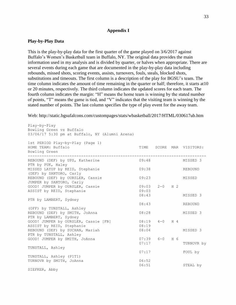
33

Appendix I

Play-by-Play Data

This is the play-by-play data for the first quarter of the game played on 3/6/2017 against

Buffalo’s Women’s Basketball team in Buffalo, NY. The original data provides the main

information used in my analysis and is divided by quarter, or halves when appropriate. There are

several events during each game that are documented in the play-by-play data including

rebounds, missed shots, scoring events, assists, turnovers, fouls, steals, blocked shots,

substitutions and timeouts. The first column is a description of the play for BGSU’s team. The

time column indicates the amount of time remaining in the quarter or half; therefore, it starts at10

or 20 minutes, respectively. The third column indicates the updated scores for each team. The

fourth column indicates the margin: “H” means the home team is winning by the stated number

of points, “T” means the game is tied, and “V” indicates that the visiting team is winning by the

stated number of points. The last column specifies the type of play event for the away team.

Web: http://static.bgsufalcons.com/custompages/stats/wbasketball/2017/HTML/030617ub.htm

Play-by-Play

Bowling Green vs Buffalo

03/06/17 5:30 pm at Buffalo, NY (Alumni Arena)

1st PERIOD Play-by-Play (Page 1)

HOME TEAM: Buffalo TIME SCORE MAR VISITORS:

Bowling Green

-----------------------------------------------------------------------------

REBOUND (DEF) by UPS, Katherine 09:48 MISSED 3

PTR by PUK, Haley

MISSED LAYUP by REID, Stephanie 09:38 REBOUND

(DEF) by SANTORO, Carly

REBOUND (DEF) by OURSLER, Cassie 09:23 MISSED

JUMPER by SANTORO, Carly

GOOD! JUMPER by OURSLER, Cassie 09:03 2-0 H 2

ASSIST by REID, Stephanie 09:03

08:43 MISSED 3

PTR by LAMBERT, Sydney

08:43 REBOUND

(OFF) by TUNSTALL, Ashley

REBOUND (DEF) by SMITH, JoAnna 08:28 MISSED 3


GOOD! JUMPER by OURSLER, Cassie [FB] 08:19 4-0 H 4

ASSIST by REID, Stephanie 08:19

REBOUND (DEF) by SUCHAN, Mariah 08:04 MISSED 3

PTR by TUNSTALL, Ashley

GOOD! JUMPER by SMITH, JoAnna 07:39 6-0 H 6

07:17 TURNOVR by

TUNSTALL, Ashley

07:17 FOUL by

TUNSTALL, Ashley (P1T1)

TURNOVR by SMITH, JoAnna 06:52

06:51 STEAL by

SIEFKER, Abby

34

06:48 MISSED

LAYUP by LAMBERT, Sydney

06:48 REBOUND

(OFF) by SANTORO, Carly

06:43 6-3 H 3 GOOD! 3

PTR by SANTORO, Carly

GOOD! LAYUP by REID, Stephanie [PNT] 06:23 8-3 H 5

REBOUND (DEF) by OURSLER, Cassie 06:10 MISSED

JUMPER by PUK, Haley

MISSED LAYUP by OURSLER, Cassie 05:41 BLOCK by

SIEFKER, Abby

05:38 REBOUND


05:33 TURNOVR by

SANTORO, Carly

MISSED 3 PTR by SMITH, JoAnna 05:21 REBOUND

(DEF) by PUK, Haley

05:01 MISSED

JUMPER by SANTORO, Carly

05:01 REBOUND

(OFF) by PUK, Haley

FOUL by OURSLER, Cassie (P1T1) 04:49

04:49 TIMEOUT

MEDIA

04:49 MISSED FT

SHOT by SIEFKER, Abby

04:49 REBOUND

(OFF) by (DEADBALL)

04:49 8-4 H 4 GOOD! FT

SHOT by SIEFKER, Abby

SUB IN : ONWUKA, Theresa 04:49

SUB IN : HEMPHILL, Summer 04:49

SUB OUT: OURSLER, Cassie 04:49

SUB OUT: UPS, Katherine 04:49

MISSED JUMPER by REID, Stephanie 04:39 REBOUND

(DEF) by PUK, Haley

04:16 TURNOVR by

SANTORO, Carly

04:16 FOUL by

SANTORO, Carly (P1T2)

MISSED 3 PTR by REID, Stephanie 03:54 REBOUND

(DEF) by PUK, Haley

03:48 TURNOVR by

PUK, Haley

STEAL by REID, Stephanie 03:47

MISSED LAYUP by SUCHAN, Mariah 03:38

REBOUND (OFF) by ONWUKA, Theresa 03:38

MISSED LAYUP by ONWUKA, Theresa 03:35 REBOUND


03:21 8-6 H 2 GOOD!

LAYUP by SIEFKER, Abby [PNT]

03:21 ASSIST by

TUNSTALL, Ashley

MISSED JUMPER by SUCHAN, Mariah 03:07 REBOUND

(DEF) by SIEFKER, Abby

REBOUND (DEF) by SMITH, JoAnna 02:59 MISSED

JUMPER by LAMBERT, Sydney

35

MISSED JUMPER by REID, Stephanie 02:49

REBOUND (OFF) by SUCHAN, Mariah 02:49

02:46 SUB IN :

THOMPSON, Caterrion

02:46 SUB IN :

CECIL, Andrea

02:46 SUB OUT:

PUK, Haley

02:46 SUB OUT:

SANTORO, Carly

GOOD! LAYUP by REID, Stephanie [PNT] 02:28 10-6 H 4

GOOD! FT SHOT by REID, Stephanie 02:28 11-6 H 5 FOUL by

THOMPSON, Caterrion (P1T3)

02:20 11-8 H 3 GOOD!

JUMPER by LAMBERT, Sydney

GOOD! FT SHOT by SUCHAN, Mariah 02:05 12-8 H 4 FOUL by

CECIL, Andrea (P1T4)

MISSED FT SHOT by SUCHAN, Mariah 02:05 REBOUND

(DEF) by CECIL, Andrea

02:05 SUB IN :

COLE, Maddie

02:05 SUB OUT:

SIEFKER, Abby

REBOUND (DEF) by SUCHAN, Mariah 01:47 MISSED

LAYUP by COLE, Maddie

TURNOVR by ONWUKA, Theresa 01:39

01:35 STEAL by

THOMPSON, Caterrion

REBOUND (DEF) by SUCHAN, Mariah 01:28 MISSED

LAYUP by TUNSTALL, Ashley

MISSED LAYUP by ONWUKA, Theresa 01:06 REBOUND

(DEF) by COLE, Maddie

STEAL by REID, Stephanie 00:51 TURNOVR by

THOMPSON, Caterrion

SUB IN : SODADE, Ayoleka 00:51 SUB IN :

SIEFKER, Abby

SUB OUT: ONWUKA, Theresa 00:51 SUB IN :

MYERS, Rachel

00:51 SUB OUT:

THOMPSON, Caterrion

00:51 SUB OUT:

COLE, Maddie

TURNOVR by SODADE, Ayoleka 00:36

00:24 12-11 H 1 GOOD! 3


00:24 ASSIST by

SIEFKER, Abby

MISSED JUMPER by REID, Stephanie 00:00 REBOUND

(DEF) by SIEFKER, Abby

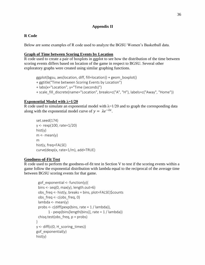
36

Appendix II

R Code

Below are some examples of R code used to analyze the BGSU Women’s Basketball data.

Graph of Time between Scoring Events by Location

R code used to create a pair of boxplots in ggplot to see how the distribution of the time between

scoring events differs based on location of the game in respect to BGSU. Several other

exploratory graphs were created using similar graphing functions.

ggplot(bgsu, aes(location, diff, fill=location)) + geom_boxplot() + ggtitle("Time between Scoring Events by Location") + labs(x="Location", y="Time (seconds)") + scale_fill_discrete(name="Location", breaks=c("A", "H"), labels=c("Away", "Home"))

Exponential Model with λ=1/20

R code used to simulate an exponential model with λ=1/20 and to graph the corresponding data

along with the exponential model curve of 𝑦 = 𝜆𝑒−𝜆𝑥.

set.seed(174) y <- rexp(100, rate=1/20) hist(y) m <- mean(y) m hist(y, freq=FALSE) curve(dexp(x, rate=1/m), add=TRUE)

Goodness-of-Fit Test

R code used to perform the goodness-of-fit test in Section V to test if the scoring events within a

game follow the exponential distribution with lambda equal to the reciprocal of the average time

between BGSU scoring events for that game.

gof_exponential <- function(y){ bins <- seq(0, max(y), length.out=6) obs_freq <- hist(y, breaks = bins, plot=FALSE)$counts obs_freq <- c(obs_freq, 0) lambda <- mean(y) probs <- c(diff(pexp(bins, rate = 1 / lambda)), 1 - pexp(bins[length(bins)], rate = 1 / lambda)) chisq.test(obs_freq, p = probs) } y <- diff(c(0, H_scoring_times)) gof_exponential(y) hist(y)

statistical analysis of momentum in basketball

Documents