statistical analysis of nmr metabolic fingerprints
TRANSCRIPT

metabolites
H
OH
OH
Review
Statistical Analysis of NMR Metabolic Fingerprints:Established Methods and Recent Advances
Helena U. Zacharias 1, Michael Altenbuchinger 2 and Wolfram Gronwald 3,* ID
1 Institute of Computational Biology, Helmholtz Zentrum München, Ingolstädter Landstraße 1,85764 Neuherberg, Germany; [email protected]
2 Statistical Bioinformatics, Institute of Functional Genomics, University of Regensburg, Am Biopark 9,93053 Regensburg, Germany; [email protected]
3 Institute of Functional Genomics, University of Regensburg, Am Biopark 9, 93053 Regensburg, Germany* Correspondence: [email protected]; Tel.: +49-941-943-5015
Received: 2 July 2018; Accepted: 18 August 2018; Published: 28 August 2018�����������������
Abstract: In this review, we summarize established and recent bioinformatic and statistical methodsfor the analysis of NMR-based metabolomics. Data analysis of NMR metabolic fingerprints exhibitsseveral challenges, including unwanted biases, high dimensionality, and typically low samplenumbers. Common analysis tasks comprise the identification of differential metabolites and theclassification of specimens. However, analysis results strongly depend on the preprocessing of thedata, and there is no consensus yet on how to remove unwanted biases and experimental varianceprior to statistical analysis. Here, we first review established and new preprocessing protocols andillustrate their pros and cons, including different data normalizations and transformations. Second,we give a brief overview of state-of-the-art statistical analysis in NMR-based metabolomics. Finally,we discuss a recent development in statistical data analysis, where data normalization becomesobsolete. This method, called zero-sum regression, builds metabolite signatures whose estimation aswell as predictions are independent of prior normalization.
Keywords: data normalization; data scaling; zero-sum; metabolic fingerprinting; NMR; statisticaldata analysis
1. Introduction
Metabolomics is defined as the comprehensive study of small organic compounds, so-calledmetabolites, in a biological specimen, e.g., a cell, an organ, or a whole organism. Particular focusis placed on the identification of metabolites that characterize specific phenotypes. These metabolicbiomarkers can facilitate new insights into pathomechanisms of diseases, as well as offer efficientdiagnostic tools and possible targets for patient treatment.
Typical metabolites are amino acids, sugars, organic acids, bases, lipids, vitamins, and variousconjugates of absorbed substances of exogenous origin. Metabolomics finds widespread application,including such diverse topics as the screening of milk of dairy cows [1] or the investigation of acutekidney injury following heart surgery [2,3].
Metabolomic investigations are mainly conducted employing hyphenated mass spectrometry ornuclear magnetic resonance (NMR) spectroscopy. Here, we will focus on the application of solutionNMR spectroscopy to biological fluids as well as tissue and cell extracts in an academic setting,although many of the described approaches are not limited to these examples.
In order to extract meaningful information from NMR metabolic fingerprints, numerous statisticaldata analysis methods are applied. Routinely, the significance of differential metabolite intensitiesis assessed by hypothesis testing. Unsupervised machine learning methods are applied to unravel
Metabolites 2018, 8, 47; doi:10.3390/metabo8030047 www.mdpi.com/journal/metabolites
Metabolites 2018, 8, 47 2 of 10
structure in the data, and supervised machine learning methods try to separate predefined groupsof specimens.
Researchers in NMR-based metabolomics are confronted with a vast amount of different methods,making it challenging to decide on one or the other. The intention of this review is twofold. First,we want to provide a brief overview of available data processing and analysis techniques, withoutthe intention of being complete. Second, we want to point the reader towards potential issues.Data analysis is not unique. Different methods yield different results, and even final conclusionscan be altered. This particularly concerns the preprocessing of data. We will review an examplewhere prior data normalization substantially influences the downstream analysis and its interpretation.Finally, we will describe a recent development where parts of the data preprocessing no longer impactdownstream analysis.
2. Preprocessing
2.1. Data Extraction
Routine statistical analysis requires predefined molecular features. These features are eitherdefined in a targeted manner, where they constitute preselected, often absolutely quantified metabolites,or in an untargeted manner, where they comprise the whole spectral region. The latter approach doesnot require the identification of metabolites prior to feature extraction, and is recommended in thecontext of exploratory phenotype analysis.
Different methods for data extraction in NMR-based metabolomics are available. In general, NMRsignal positions can vary across specimens due to differences in pH, ionic strength, or measurementtemperature. A widely used and robust method to at least partially compensate for these effects isspectral binning. A simple but efficient strategy implies the splitting of the whole spectral regioninto equally spaced buckets/bins. Data points inside every bucket are summed up or integrated.The whole dataset is then represented as a matrix of bucket integrals, where the rows correspond toindividual specimens and the columns correspond to individual bins, respectively. Other schemessuch as adaptive binning [4], spectral alignment [5,6], and combinations thereof have been shown tobe superior to equidistant binning [4,5,7–9].
2.2. Normalization
Metabolomic datasets are prone to unwanted technical and/or biological variances and biases.Technical variances can result from differences in sample collection, storage, and preparation, aswell as spectrometer performance across the set of investigated specimens. Unintended biologicalvariances can arise due to numerous reasons. The most prominent, in the case of urine metabolomics,are dilutions of metabolite concentrations due to the varying fluid intake of study participants.Urine specimen dilutions can further vary due to drugs, toxins, disease status, respiration, defecation,perspiration, and patient treatment [10,11]. Other reasons for unintended biological variances may bedifferences in the available sample volumes due to unequal numbers of cells in the case of cell-lineextracts, varying tissue volumes/masses, or varying biofluid volumes across the investigated cohort.
To minimize the undesired technical and biological variance across specimens is the goal of datanormalization in metabolomics. As stated by Craig et al. (2006) [10], it can be considered as a rowoperation to remove unwanted sample-to-sample variations. Numerous normalization methods havebeen suggested during the past years, and we will briefly introduce the most prominent strategies forNMR-based metabolomics.
A normalization of each metabolic fingerprint to a specific “housekeeping” metabolite,e.g., creatinine, is a common approach to remove data variances due to differences in overall urineconcentrations [10,12], as exemplified in Figure 1. Here, creatinine clearance is assumed to beconstant and used as a proxy for renal function [10]. However, this normalization strategy cannot berecommended in general [12]. It assumes the absence of interindividual differences in the production

Metabolites 2018, 8, 47 3 of 10
and renal excretion of creatinine [13]. However, creatinine production and excretion depend on the sex,age, muscle mass, diet, and pregnancy, as well as renal pathology of the examined individual [14,15].
Metabolites 2018, 8, x 3 of 10
depend on the sex, age, muscle mass, diet, and pregnancy, as well as renal pathology of the examined individual [14,15].
Figure 1. Normalization of two different urine spectra with respect to creatinine. (Left) Before normalization and (right) after normalization.
Another commonly applied method to reduce unwanted sample-to-sample variation is the normalization of every spectrum to a total sum of one, the so-called total spectral intensity/area normalization. Here, each metabolic feature is divided by the total sum of all of the spectral features. It assumes that only a relatively small amount of metabolites is regulated in approximately equal shares up and down, while all others remain constant. However, this prerequisite is often not fulfilled, especially in the case of kidney diseases where, e.g., higher overall blood metabolite levels are observed in diseased than in healthy patients [3].
Probabilistic quotient normalization (PQN) assumes that biologically interesting concentration changes only affect parts of the NMR spectrum, whereas different specimen dilutions influence all of the metabolite signals simultaneously [16]. For PQN, each spectrum first is normalized to the total spectral intensity, and multiplied by 100. Subsequently, a reference spectrum, e.g., the median spectrum over all of the spectra of a cohort is derived, and the quotient of all of the variables of the investigated spectra and the reference spectrum is calculated. In the next step, the median of these quotients across all of the metabolic features is computed, and finally, each metabolic feature of the spectra is divided by this median. Again, this normalization method is not applicable if the underlying assumptions are not fulfilled.
If only technical variances due to differences in spectrometer performance need to be addressed, a normalization to the NMR reference substance is recommended [3].
We systematically compared established and advanced normalization methods for urinary metabolomic NMR datasets [17]. Here, quantile [18], variance stabilization [19] and cubic spline [20] normalization performed best with respect to sample classification, bias reduction, and the detection of correct fold changes. However, these methods all assume that only a relatively small proportion of the metabolites is different between the investigated groups, and therefore, the average total spectral areas are assumed to be similar across specimens and groups [21]. If this assumption is not fulfilled, Hochrein et al. 2005 [21] suggest to learn the normalization parameters on a subset of non-regulated features only. Additionally, it is important to note that all of the different normalization strategies mentioned here impact the following analysis steps such as screening for differential metabolites or multivariate metabolic signatures [22–25], as we will discuss in more detail in the following sections.
2.3. Additional Data Transformation
In addition to normalization, further data transformations might be necessary. Many statistical methods assume variables that are distributed multivariate normal and have constant variance. Binned NMR intensities frequently exhibit skewed distributions across specimens, i.e., the data are
Figure 1. Normalization of two different urine spectra with respect to creatinine. (Left) Beforenormalization and (right) after normalization.
Another commonly applied method to reduce unwanted sample-to-sample variation is thenormalization of every spectrum to a total sum of one, the so-called total spectral intensity/areanormalization. Here, each metabolic feature is divided by the total sum of all of the spectral features.It assumes that only a relatively small amount of metabolites is regulated in approximately equalshares up and down, while all others remain constant. However, this prerequisite is often not fulfilled,especially in the case of kidney diseases where, e.g., higher overall blood metabolite levels are observedin diseased than in healthy patients [3].
Probabilistic quotient normalization (PQN) assumes that biologically interesting concentrationchanges only affect parts of the NMR spectrum, whereas different specimen dilutions influence allof the metabolite signals simultaneously [16]. For PQN, each spectrum first is normalized to thetotal spectral intensity, and multiplied by 100. Subsequently, a reference spectrum, e.g., the medianspectrum over all of the spectra of a cohort is derived, and the quotient of all of the variables of theinvestigated spectra and the reference spectrum is calculated. In the next step, the median of thesequotients across all of the metabolic features is computed, and finally, each metabolic feature of thespectra is divided by this median. Again, this normalization method is not applicable if the underlyingassumptions are not fulfilled.
If only technical variances due to differences in spectrometer performance need to be addressed,a normalization to the NMR reference substance is recommended [3].
We systematically compared established and advanced normalization methods for urinarymetabolomic NMR datasets [17]. Here, quantile [18], variance stabilization [19] and cubic spline [20]normalization performed best with respect to sample classification, bias reduction, and the detectionof correct fold changes. However, these methods all assume that only a relatively small proportion ofthe metabolites is different between the investigated groups, and therefore, the average total spectralareas are assumed to be similar across specimens and groups [21]. If this assumption is not fulfilled,Hochrein et al. 2005 [21] suggest to learn the normalization parameters on a subset of non-regulatedfeatures only. Additionally, it is important to note that all of the different normalization strategiesmentioned here impact the following analysis steps such as screening for differential metabolites ormultivariate metabolic signatures [22–25], as we will discuss in more detail in the following sections.
Metabolites 2018, 8, 47 4 of 10
2.3. Additional Data Transformation
In addition to normalization, further data transformations might be necessary. Many statisticalmethods assume variables that are distributed multivariate normal and have constant variance.Binned NMR intensities frequently exhibit skewed distributions across specimens, i.e., the dataare heteroscedastic. The most prominent method to achieve approximately normal distributedvariables and equal variance is the logarithmic transformation, which was suggested in the context ofNMR-based metabolomics, e.g., by Viant et al. (2005) [26]. A mathematically more evolved method,which requires the estimation of an additional parameter, is a variance stabilizing transformation(VST) [27]. VST in combination with normalization is variance stabilization normalization (VSN) [19].This method was systematically evaluated in Kohl et al. (2012) [17], where it was among the bestpreprocessing strategies and particularly performed well for both classification and bias removal.Other data transformations that do not account for heteroscedasticity but which correct the variance ofvariables are, e.g., Pareto [28] and autoscaling [29]. Both methods rescale metabolite features; thus, theyare column operations in contrast to normalization, which is a row operation according to Craig et al.(2006) [10]. A detailed discussion of these strategies is beyond the scope of this article and we referthe interested reader for example to Craig et al. (2006) [10], Kohl et al. (2012) [17], Gromski et al.(2015) [23], van den Berg et al. (2006) [30], and Emwas et al. (2018) [31] for more details.
3. Statistical Data Analysis Strategies
3.1. Unsupervised Machine Learning Methods
In unsupervised machine learning, no information about underlying groups is used. Therefore,the group separations that are observed are purely data-driven. Unsupervised algorithms are oftenemployed to check for group separation prior to the classification of data or in cases where too fewsamples are available for classification with rigid cross-validation.
One of the most prominent unsupervised methods in the metabolomics community is principalcomponent analysis (PCA). PCA is a dimension reduction approach where new coordinate axes inthe directions of maximal variances are drawn. The maximum variance is not necessarily equal tothe intended biological variance, i.e., the metabolic differences between different phenotypes, butmight also arise from for example batch effects, which had not been successfully removed by datanormalization. PCA enables the easy visualization of high-dimensional data. Closely related to PCA isindependent component analysis (ICA), which has been shown to provide good results for metabolicdata [32,33].
Other used methods include clustering approaches such as hierarchical clustering [34],non-hierarchical clustering employing the k-means method [35], and clustering by affinity propagation [36].Self-organizing maps are a widely used method for two-dimensional data visualization [37]. For moredetails about unsupervised machine learning in the context of NMR-based metabolomics, we refer theinterested reader for example to Zacharias et al. (2013) [38].
3.2. Hypothesis Testing
Hypothesis tests are of central importance in metabolomics data analysis. They are used toidentify differentially regulated metabolites. For instance, a standard application is to screen formetabolites that serve as biomarkers of a certain disease. Here, metabolite intensities are comparedbetween healthy and diseased individuals. Routinely, in the case of normally distributed data, this isdone by applying a Student’s t-test or, if there are more than two conditions to be compared, an analysisof variance (ANOVA).
Since common metabolic studies comprise a large number of metabolic features, significance levelsor p-values need to be corrected for multiple hypothesis testing. Prominent methods are controllingthe false discovery rate according to Benjamini and Hochberg [39] and controlling the familywise errorrate according to Bonferroni [40].

Metabolites 2018, 8, 47 5 of 10
However, the results of univariate data analysis exhibit a distinct dependency on the a priorichosen normalization method, as investigated by Zacharias et al. (2017) [22]. Figure 2 illustrates theseobservations for a t-test analysis of urinary NMR fingerprints of acute kidney injury (AKI) versushealthy patients.Metabolites 2018, 8, x 5 of 10
Figure 2. Test for differentially regulated metabolites in 1D 1H urinary nuclear magnetic resonance (NMR) fingerprints between acute kidney injury (AKI) and healthy patients with respect to different normalization strategies. –Log10(p-values) of moderated t-test analysis are shown after preprocessing with four different normalization methods: scaling to (a) equal total spectral area, (b) scaling to creatinine, (c) probabilistic quotient normalization (PQN), and (d) scaling to the internal reference TSP, plotted versus the ppm regions of the corresponding NMR buckets (upper panels). The significance level for Benjamini–Hochberg (B/H) adjusted p-values below 0.01, corresponding to a false discovery rate (FDR) below 1%, is marked by an orange line, and the significant NMR features are indicated as orange diamonds. The corresponding log2 fold changes (log2 FC) plotted versus the ppm regions are shown in the lower panels (e–h). Since log2 FCs were calculated as AKI minus non-AKI, positive log2 FCs correspond to higher values in AKI than in non-AKI samples. Figure adapted from Zacharias et al. (2017) [22].
The number as well as the identity of statistically significant NMR buckets strongly depends on the employed normalization strategy. This finding points to an inherent problem of standard statistical data analysis in metabolomics studies: the respective results are always dependent on the often arbitrarily chosen normalization strategy, and findings can probably only be reproduced if the initial choice of normalization is used.
3.3. Supervised Machine Learning Methods
The classification of an unknown sample into two or more known phenotypic classes (e.g., healthy and diseased) is a common task for which techniques from machine learning are used.
Popular machine learning methods in omics science are partial least squares discriminant analysis (PLS-DA) [41], orthogonal projection to latent structures discriminant analysis (OPLS-DA) [42], random forest (RF) [43], support vector machine (SVM) [44], as well as least-absolute shrinkage and selection operator (LASSO) [45], ridge [46], and elastic net regression [47].
In metabolomic data analysis, PLS-DA and OPLS-DA are most widely used. RF and SVM are less frequently applied, but are well established, for example, in gene expression analysis. Hochrein et al. (2012) [48] showed that RFs are particularly well suited for the analysis of high-dimensional NMR data with regard to prediction accuracy [48]. Elastic net, or its special cases ridge and LASSO regression, are also rather unpopular in metabolomics data analysis. However, they are very popular in the machine learning community, and exhibit excellent performance also in NMR metabolomics [48]. All methods have their pros and cons, and several comprehensive comparisons are available, e.g., Hochrein et al. (2012), [48], Gromski et al. (2015) [49], Ren et al. (2015) [50], and Cuperlovic-Culf et al. (2018) [51].
A particular challenge in supervised machine learning is the high-dimensionality of the data. Usually, many more metabolic features are assessed than specimens are available. As a consequence, high performance on the training data does not necessarily imply high performance on the test data,
02
46
8
Total Area
ppm
−log
10 (p−v
alue
)
(a)
9 8 7 6 5 4 3 2 1
02
46
8
Creatinine
ppm
−log
10 (p−v
alue
)
(b)
9 8 7 6 5 4 3 2 1
02
46
8
PQN
ppm
−log
10 (p−v
alue
)
(c)
9 8 7 6 5 4 3 2 1
02
46
8
TSP
ppm
−log
10 (p−v
alue
)
(d)
9 8 7 6 5 4 3 2 1
−1.5
−0.5
0.5
1.5
Total Area
ppm
log 2
FC
(e)
9 8 7 6 5 4 3 2 1
−1.5
−0.5
0.5
1.5
Creatinine
ppm
log 2
FC
(f)
9 8 7 6 5 4 3 2 1
−1.5
−0.5
0.5
1.5
PQN
ppm
log 2
FC
(g)
9 8 7 6 5 4 3 2 1
−1.5
−0.5
0.5
1.5
TSP
ppm
log 2
FC
(h)
9 8 7 6 5 4 3 2 1
Figure 2. Test for differentially regulated metabolites in 1D 1H urinary nuclear magnetic resonance(NMR) fingerprints between acute kidney injury (AKI) and healthy patients with respect to differentnormalization strategies. –Log10(p-values) of moderated t-test analysis are shown after preprocessingwith four different normalization methods: scaling to (a) equal total spectral area, (b) scaling tocreatinine, (c) probabilistic quotient normalization (PQN), and (d) scaling to the internal reference TSP,plotted versus the ppm regions of the corresponding NMR buckets (upper panels). The significancelevel for Benjamini–Hochberg (B/H) adjusted p-values below 0.01, corresponding to a false discoveryrate (FDR) below 1%, is marked by an orange line, and the significant NMR features are indicated asorange diamonds. The corresponding log2 fold changes (log2 FC) plotted versus the ppm regions areshown in the lower panels (e–h). Since log2 FCs were calculated as AKI minus non-AKI, positive log2
FCs correspond to higher values in AKI than in non-AKI samples. Figure adapted from Zacharias et al.(2017) [22].
The number as well as the identity of statistically significant NMR buckets strongly dependson the employed normalization strategy. This finding points to an inherent problem of standardstatistical data analysis in metabolomics studies: the respective results are always dependent on theoften arbitrarily chosen normalization strategy, and findings can probably only be reproduced if theinitial choice of normalization is used.
3.3. Supervised Machine Learning Methods
The classification of an unknown sample into two or more known phenotypic classes (e.g., healthyand diseased) is a common task for which techniques from machine learning are used.
Popular machine learning methods in omics science are partial least squares discriminant analysis(PLS-DA) [41], orthogonal projection to latent structures discriminant analysis (OPLS-DA) [42], randomforest (RF) [43], support vector machine (SVM) [44], as well as least-absolute shrinkage and selectionoperator (LASSO) [45], ridge [46], and elastic net regression [47].
In metabolomic data analysis, PLS-DA and OPLS-DA are most widely used. RF and SVM are lessfrequently applied, but are well established, for example, in gene expression analysis. Hochrein et al.(2012) [48] showed that RFs are particularly well suited for the analysis of high-dimensional NMR datawith regard to prediction accuracy [48]. Elastic net, or its special cases ridge and LASSO regression, arealso rather unpopular in metabolomics data analysis. However, they are very popular in the machine
Metabolites 2018, 8, 47 6 of 10
learning community, and exhibit excellent performance also in NMR metabolomics [48]. All methodshave their pros and cons, and several comprehensive comparisons are available, e.g., Hochrein et al.(2012), [48], Gromski et al. (2015) [49], Ren et al. (2015) [50], and Cuperlovic-Culf et al. (2018) [51].
A particular challenge in supervised machine learning is the high-dimensionality of the data.Usually, many more metabolic features are assessed than specimens are available. As a consequence,high performance on the training data does not necessarily imply high performance on the test data,which is commonly known as the problem of over-fitting. Therefore, results need to be validatedby bootstrapping, cross-validation, or in the best case, on independent validation data. Althoughstate-of-the-art machine learning methods are designed to control over-fitting, such as LASSO/ridgeregression, SVMs, and random forests, their performance remains to be validated.
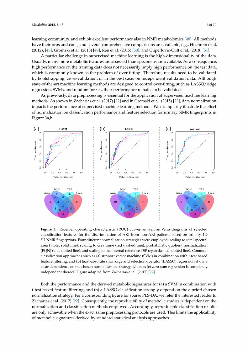
As previously, data preprocessing is essential for the application of supervised machine learningmethods. As shown in Zacharias et al. (2017) [22] and in Gromski et al. (2015) [23], data normalizationimpacts the performance of supervised machine learning methods. We exemplarily illustrate the effectof normalization on classification performance and feature selection for urinary NMR fingerprints inFigure 3a,b.
Metabolites 2018, 8, x 6 of 10
which is commonly known as the problem of over-fitting. Therefore, results need to be validated by
bootstrapping, cross-validation, or in the best case, on independent validation data. Although
state-of-the-art machine learning methods are designed to control over-fitting, such as LASSO/ridge
regression, SVMs, and random forests, their performance remains to be validated.
As previously, data preprocessing is essential for the application of supervised machine
learning methods. As shown in Zacharias et al. (2017) [22] and in Gromski et al. (2015) [23], data
normalization impacts the performance of supervised machine learning methods. We exemplarily
illustrate the effect of normalization on classification performance and feature selection for urinary
NMR fingerprints in Figure 3a,b.
Figure 3. Receiver operating characteristic (ROC) curves as well as Venn diagrams of selected
classification features for the discrimination of AKI from non-AKI patients based on urinary 1D 1H
NMR fingerprints. Four different normalization strategies were employed: scaling to total spectral
area (violet solid line), scaling to creatinine (red dashed line), probabilistic quotient normalization
(PQN) (blue dotted line), and scaling to the internal reference TSP (cyan dashed–dotted line).
Common classification approaches such as (a) support vector machine (SVM) in combination with
t-test based feature filtering, and (b) least-absolute shrinkage and selection operator (LASSO)
f−SVM
False positive rate
Tru
e po
siti
ve
rate
0.0 0.2 0.4 0.6 0.8 1.0
0.0
0.2
0.4
0.6
0.8
1.0
(a) LASSO
False positive rate
Tru
e po
siti
ve
rate
0.0 0.2 0.4 0.6 0.8 1.0
0.0
0.2
0.4
0.6
0.8
1.0
(b) zero−sum
False positive rate
Tru
e po
siti
ve
rate
0.0 0.2 0.4 0.6 0.8 1.00.0
0.2
0.4
0.6
0.8
1.0
(c)
10
39
2
30
0
27
6
33
80 0
5
35
0
Area Crea.
PQN TSP
71
4
1
7
40
7
0
10
21 0
2
7
3
Area Crea.
PQN TSP
00
0
0
1
67
0
0
0
00 0
0
0
0
Area Crea.
PQN TSP
Figure 3. Receiver operating characteristic (ROC) curves as well as Venn diagrams of selectedclassification features for the discrimination of AKI from non-AKI patients based on urinary 1D1H NMR fingerprints. Four different normalization strategies were employed: scaling to total spectralarea (violet solid line), scaling to creatinine (red dashed line), probabilistic quotient normalization(PQN) (blue dotted line), and scaling to the internal reference TSP (cyan dashed–dotted line). Commonclassification approaches such as (a) support vector machine (SVM) in combination with t-test basedfeature filtering, and (b) least-absolute shrinkage and selection operator (LASSO) regression show aclear dependence on the chosen normalization strategy, whereas (c) zero-sum regression is completelyindependent thereof. Figure adapted from Zacharias et al. (2017) [22].
Both the performance and the derived metabolic signatures for (a) a SVM in combination witht-test based feature filtering, and (b) a LASSO classification strongly depend on the a priori chosennormalization strategy. For a corresponding figure for sparse PLS-DA, we refer the interested reader toZacharias et al. (2017) [22]. Consequently, the reproducibility of metabolic studies is dependent on thenormalization and classification methods employed. Accordingly, reproducible classification resultsare only achievable when the exact same preprocessing protocols are used. This limits the applicabilityof metabolic signatures derived by standard statistical analysis approaches.

Metabolites 2018, 8, 47 7 of 10
4. Zero-Sum Regression
To overcome these limits of traditional biomarker signatures, zero-sum regression [52,53], whichhas recently been demonstrated to be invariant under any normalization of data [53], has beenextended to logistic zero-sum regression [22]. In contrast to commonly used approaches, logisticzero-sum regression always selects the same set of biomarkers for sample classification, regardless ofthe chosen normalization method. Therefore, prior data normalization may be omitted completely.
In brief, it is based on the following concept: We start with the binned fingerprinting data xij,where xij is the logarithm of the intensity of bin j ∈ {1, . . . ,p} in spectrum i ∈ {1, . . . ,N}, and yi is thecorresponding (clinical) response of patient i. In standard regression analysis, prior data normalizationto a common unit such as the total spectral area is required. As the data are on a logarithmic scale,normalization to a common unit becomes a shifting of the binned value xij by some spectrum-specificvalue γi. Therefore, in the case of normalized data, the regression equation reads:
yi = β0 +p
∑j=1
β j(xij + γi
)+ εi (1)
Equation (1) becomes independent of the normalization factor γi if and only if the regressioncoefficients βj sum up to zero, i.e.:
p
∑j=1
β j = 0. (2)
As a consequence, the additional constraint that all regression coefficients have to sum up to zerois set in zero-sum regression. Zacharias et al. (2017) [22] showed for two metabolomic datasets that theobtained biomarker signatures were indeed independent of any prior data normalization. Figure 3cillustrates these results for a urinary 1D 1H NMR metabolic dataset.
5. Available Software for Metabolomics Data Preprocessing and Statistical Analysis
The statistical programming environment R [54] provides a convenient way of normalizing andtransforming datasets, as well as performing subsequent data analysis. Other common tools to performthese tasks or parts thereof include, for example, the numerical programming environment MATLAB(The MathWorks Inc., Natick, MA, USA), the online server MetaboAnalyst [55], MVAPACK [56],Workflow4Metabolomics [57], and the data analysis software SIMCA (Umetrics, Umeå, Sweden). Mostrecently, NormalizeMets has been proposed for the comparative evaluation of normalization methodsin metabolomics studies [58]. Another web tool, called MetaPre, offers the possibility of evaluating thenormalization performance of, in total, 16 different normalization methods [59]. Logistic as well aslinear zero-sum regression are available as an R package and as high-performance computing softwareat https://github.com/rehbergT/zeroSum.
6. Conclusions
In this review, we focused on the statistical data analysis of NMR-derived metabolic fingerprints.Special emphasis was given to the issue of data normalization and its impact on downstream analysisand result interpretation. In this context, we focused on the novel logistic zero-sum regression methodthat is independent of prior data normalization, and therefore has the potential to greatly enhance thereproducibility of biomarker studies.
Funding: This work was supported by e:Med initiative of the German Ministry for Education and Research[grant 031A428A].
Conflicts of Interest: The authors declare no conflict of interest.
Metabolites 2018, 8, 47 8 of 10
References
1. Klein, M.S.; Buttchereit, N.; Miemczyk, S.P.; Immervoll, A.K.; Louis, C.; Wiedemann, S.; Junge, W.; Thaller, G.;Oefner, P.J.; Gronwald, W. NMR metabolomic analysis of dairy cows reveals milk glycerophosphocholineto phosphocholine ratio as prognostic biomarker for risk of ketosis. J. Proteome Res. 2012, 11, 1373–1381.[CrossRef] [PubMed]
2. Zacharias, H.U.; Schley, G.; Hochrein, J.; Klein, M.S.; Köberle, C.; Eckardt, K.U.; Willam, C.; Oefner, P.J.;Gronwald, W. Analysis of Human Urine Reveals Metabolic Changes Related to the Development of AcuteKidney Injury Following Cardiac Surgery. Metabolomics 2013, 9, 697–707. [CrossRef]
3. Zacharias, H.U.; Hochrein, J.; Vogl, F.C.; Schley, G.; Mayer, F.; Jeleazcov, C.; Eckardt, K.-U.; Willam, C.;Oefner, P.J.; Gronwald, W. Identification of Plasma Metabolites Prognostic of Acute Kidney Injury afterCardiac Surgery with Cardiopulmonary Bypass. J. Proteome Res. 2015, 14, 2897–2905. [CrossRef] [PubMed]
4. Davis, R.A.; Charlton, A.J.; Godward, J.; Jones, S.A.; Harrison, M.; Wilson, J.C. Adaptive binning: An improvedbinning method for metabolomics data using the undecimated wavelet transform. Chemom. Intell. Lab. 2007, 85,144–154. [CrossRef]
5. Vu, T.N.; Laukens, K. Getting your peaks in line: A review of alignment methods for NMR spectral data.Metabolites 2013, 3, 259–276. [CrossRef] [PubMed]
6. Savorani, F.; Tomasi, G.; Engelsen, S.B. Icoshift: A versatile Tool for the Rapid Alignment of 1D NMR Spectra.J. Magn. Reson. 2010, 202, 190–202. [CrossRef] [PubMed]
7. De Meyer, T.; Sinnaeve, D.; van Gasse, B.; Rietzschel, E.R.; de Buyzere, M.L.; Langlois, M.R.; Bekaert, S.;Martins, J.C.; van Criekinge, W. Evaluation of Standard and Advanced Preprocessing Methods for theUnivariate Analysis of Blood Serum 1H-NMR Spectra. Anal. Bioanal. Chem. 2010, 398, 1781–1790. [CrossRef][PubMed]
8. Anderson, P.E.; Reo, N.V.; DelRaso, N.J.; Doom, T.E.; Raymer, M.L. Gaussian binning: A new kernel-basedmethod for processing NMR spectroscopic data for metabolomics. Metabolomics 2008, 4, 261–272. [CrossRef]
9. Sousa, S.; Magalhães, A.; Ferreira, M.M.C. Optimized bucketing for NMR spectra: Three case studies.Chemom. Intell. Lab. 2013, 122, 93–102. [CrossRef]
10. Craig, A.; Cloarec, O.; Holmes, E.; Nicholson, J.K.; Lindon, J.C. Scaling and Normalization Effects in NMRSpectroscopic Metabolomic Data Sets. Anal. Chem. 2006, 78, 2262–2267. [CrossRef] [PubMed]
11. Ryan, D.; Robards, K.; Prenzler, P.D.; Kendall, M. Recent and potential developments in the analysis of urine:A review. Anal. Chim. Acta 2011, 684, 8–20. [CrossRef] [PubMed]
12. Lindon, J.C.; Nicholson, J.K.; Holmes, E. (Eds.) The Handbook of Metabonomics and Metabolomics. NMRSpectroscopy Techniques for Application to Metabonomics; Elsevier: Amsterdam, The Netherlands, 2007.
13. Waikar, S.S.; Sabbisetti, V.S.; Bonventre, J.V. Normalization of Urinary Biomarkers to Creatinine duringChanges in Glomerular Filtration Rate. Kidney Int. 2010, 78, 486–494. [CrossRef] [PubMed]
14. Curhan, G. Cystatin C: A Marker for Renal Function of Something More? Clin. Chem. 2005, 51, 293–294.[CrossRef] [PubMed]
15. Stevens, L.A.; Levey, A.S. Measured GFR as a confirmatory test for estimated GFR. J. Am. Soc. Nephrol. 2009,20, 2305–2313. [CrossRef] [PubMed]
16. Dieterle, F.; Ross, A.; Schlotterbeck, G.; Senn, H. Probabilistic Quotient Normalization as Robust Method toAccount for Dillution of Complex Biological Mixtures. Application to 1H NMR Metabolomics. Anal. Chem.2006, 78, 4281–4290. [CrossRef] [PubMed]
17. Kohl, S.M.; Klein, M.S.; Hochrein, J.; Oefner, P.J.; Spang, R.; Gronwald, W. State-of-the Art Data NormalizationMethods Improve NMR-Based Metabolomic Analysis. Metabolomics 2012, 8, 146–160. [CrossRef] [PubMed]
18. Bolstad, B.M.; Irizarry, R.A.; Astrand, M.; Speed, T.P. A Comparison of Normalization Methods for HighDensity Oligonucleotide Array Data Based on Variance and Bias. Bioinformatics 2003, 19, 185–193. [CrossRef][PubMed]
19. Huber, W.; Heydebreck, A.V.; Sültmann, H.; Poustka, A.; Vingron, M. Variance Stabilisation Applied toMicroarray Data Calibration and to the Quantification of Differential Expression. Bioinformatics 2002, 18,S96–S104. [CrossRef] [PubMed]
20. Workman, C.; Jensen, L.J.; Jarmer, H.; Berka, R.; Gautier, L.; Nielser, H.B.; Saxild, H.H.; Nielsen, C.; Brunak, S.;Knudsen, S. A New Non-Linear Normalization Method for Reducing Variability in DNA MicroarrayExperiments. Genome Biol. 2002, 3. [CrossRef]
Metabolites 2018, 8, 47 9 of 10
21. Hochrein, J.; Zacharias, H.U.; Taruttis, F.; Samol, C.; Engelmann, J.C.; Spang, R.; Oefner, P.J.; Gronwald, W.Data Normalization of 1H NMR Metabolite Fingerprinting Data Sets in the Presence of UnbalancedMetabolite Regulation. J. Proteome Res. 2015, 14, 3217–3228. [CrossRef] [PubMed]
22. Zacharias, H.U.; Rehberg, T.; Mehrl, S.; Richtmann, D.; Wettig, T.; Oefner, P.J.; Spang, R.; Gronwald, W.;Altenbuchinger, M. Scale-invariant biomarker discovery in urine and plasma metabolite fingerprints.J. Proteome Res. 2017, 16, 3596–3605. [CrossRef] [PubMed]
23. Gromski, P.S.; Xu, Y.; Hollywood, K.A.; Turner, M.L.; Goodacre, R. The influence of scaling metabolomicsdata on model classification accuracy. Metabolomics 2015, 11, 684–695. [CrossRef]
24. Jauhiainen, A.; Madhu, B.; Narita, M.; Narita, M.; Griffiths, J.; Tavaré, S. Normalization of metabolomics datawith applications to correlation maps. Bioinformatics 2014, 30, 2155–2161. [CrossRef] [PubMed]
25. Saccenti, E. Correlation Patterns in Experimental Data Are Affected by Normalization Procedures:Consequences for Data Analysis and Network Inference. J. Proteome Res. 2017, 16, 619–634. [CrossRef][PubMed]
26. Viant, M.R.; Lyeth, B.G.; Miller, M.G.; Berman, R.F. An NMR metabolomic investigation of early metabolicdisturbances following traumatic brain injury in a mammalian model. NMR Biomed. 2005, 18, 507–516.[CrossRef] [PubMed]
27. Purohit, P.V.; Rocke, D.M.; Viant, M.R.; Woodruff, D.L. Discrimination models using variance-stabilizingtransformation of metabolomic NMR data. Omics 2004, 8, 118–130. [CrossRef] [PubMed]
28. Eriksson, L.; Antti, H.; Gottfries, J.; Holmes, E.; Johansson, E.; Lindgren, F.; Long, I.; Lundstedt, T.;Trygg, J.; Wold, S. Using Chemometrics for Navigating in the Large Data Sets of Genomics, Proteomics, andMetabonomics (gpm). Anal. Bioanal. Chem. 2004, 380, 419–429. [CrossRef] [PubMed]
29. Jackson, J.E. A User’s Guide to Principal Components; Wiley-Interscience: Hoboken, NJ, USA, 2003.30. Van den Berg, R.A.; Hoefsloot, H.C.; Westerhuis, J.A.; Smilde, A.K.; van der Werf, M.J. Centering, scaling,
and transformations: Improving the biological information content of metabolomics data. BMC Genom. 2006,7, 142. [CrossRef] [PubMed]
31. Emwas, A.-H.; Saccenti, E.; Gao, X.; McKay, R.T.; dos Santos, V.A.M.; Roy, R.; Wishart, D.S. Recommendedstrategies for spectral processing and post-processing of 1D 1H-NMR data of biofluids with a particularfocus on urine. Metabolomics 2018, 14, 31. [CrossRef] [PubMed]
32. Scholz, M.; Gatzek, S.; Sterling, A.; Fiehn, O.; Selbig, J. Metabolite Fingerprinting: Detecting BiologicalFeatures by Independent Component Analysis. Bioinformatics 2004, 20, 2447–2454. [CrossRef] [PubMed]
33. Klein, M.S.; Dorn, C.; Saugspier, M.; Hellerbrand, C.; Oefner, P.J.; Gronwald, W. Discrimination of Steatosisand NASH in Mice Using Nuclear Magnetic Resonance Spectroscopy. Metabolomics 2011, 7, 237–246.[CrossRef]
34. Draisma, H.H.; Reijmers, T.H.; van der Kloet, F.; Bobeldijk-Pastorova, I.; Spies-Faber, E.; Vogels, J.T.;Meulman, J.J.; Boomsma, D.I.; van der Greef, J.; Hankemeier, T. Equating, or correction for between-blockeffects with application to body fluid LC-MS and NMR metabolomics data sets. Anal. Chem. 2010, 82,1039–1046. [CrossRef] [PubMed]
35. Hartigan, J. Clustering Algorithms; John Wiley: New York, NY, USA, 1975.36. Frey, B.J.; Dueck, D. Clustering by passing messages between data points. Science 2007, 315, 972–976.
[CrossRef] [PubMed]37. Dow, L.K.; Sandeep, K.; Dow, E.R. Self-organizing Maps for the Analysis of NMR Spectra. Biosilico 2004, 2,
157–163. [CrossRef]38. Zacharias, H.U.; Hochrein, J.; Klein, M.S.; Samol, C.; Oefner, P.J.; Gronwald, W. Current Experimental,
Bioinformatic and Statistical Methods used in NMR Based Metabolomics. Curr. Metabol. 2013, 1, 253–268.[CrossRef]
39. Benjamini, Y.; Hochberg, Y. Controlling the False Discovery Rate: A Practical and Powerful Approach toMultiple Testing. J. R. Stat. Soc. B 1995, 57, 289–300.
40. Salkind, N.J. (Ed.) Bonferroni and Sidak Corrections for Multiple Comparisons. In Encyclopedia of Measurementand Statistics; Sage: Thousand Oaks, CA, USA, 2007.
41. Barker, M.; Rayens, W. Partial Least Squares for Discrimination. J. Chemom. 2003, 17, 166–173. [CrossRef]42. Trygg, J.; Wold, S. Orthogonal Projections to Latent Structures. J. Chemom. 2002, 16, 119–128. [CrossRef]43. Breiman, L. Random Forests. Mach. Learn. 2001, 45, 5–32. [CrossRef]
Metabolites 2018, 8, 47 10 of 10
44. Burges, C.J.C. A Tutorial on Support Vector Machines for Pattern Recognition. Data Min. Knowl. Discov. 1998,2, 121–167. [CrossRef]
45. Tibshirani, R. Regression Shrinkage and Selection via the Lasso. J. R. Stat. Soc. B 1996, 58, 267–288.46. Hoerl, A.E.; Kennard, R.W. Ridge Regression: Biased Estimation for Nonorthogonal Problems. Technometrics
1970, 12, 55–67. [CrossRef]47. Zou, H.; Hastie, T. Regularization and Variable Selection via the Elastic Net. J. R. Stat. Soc. B 2005, 67,
301–320. [CrossRef]48. Hochrein, J.; Klein, M.S.; Zacharias, H.U.; Li, J.; Wijffels, G.; Schirra, H.J.; Spang, R.; Oefner, P.J.; Gronwald, W.
Performance Evaluation of Algorithms for the Classification of Metabolic 1H-NMR Fingerprints. J. Proteome Res.2012, 11, 6242–6251. [CrossRef] [PubMed]
49. Gromski, P.S.; Muhamadali, H.; Ellis, D.I.; Xu, Y.; Correa, E.; Turner, M.L.; Goodacre, R. A tutorial review:Metabolomics and partial least squares-discriminant analysis—A marriage of convenience or a shotgunwedding. Anal. Chim. Acta 2015, 879, 10–23. [CrossRef] [PubMed]
50. Ren, S.; Hinzman, A.A.; Kang, E.L.; Szczesniak, R.D.; Lu, L.J. Computational and statistical analysis ofmetabolomics data. Metabolomics 2015, 11, 1492–1513. [CrossRef]
51. Cuperlovic-Culf, M. Machine Learning Methods for Analysis of Metabolic Data and Metabolic PathwayModeling. Metabolites 2018, 8, 4. [CrossRef] [PubMed]
52. Lin, W.; Shi, P.; Feng, R.; Li, H. Variable selection in regression with compositional covariates. Biometrika2014, 101, 785–797. [CrossRef]
53. Altenbuchinger, M.; Rehberg, T.; Zacharias, H.U.; Stämmler, F.; Dettmer, K.; Weber, D.; Hiergeist, A.;Gessner, A.; Holler, E.; Oefner, P.J.; et al. Reference point insensitive molecular data analysis. Bioinformatics2017, 33, 219–226. [CrossRef] [PubMed]
54. Development Core Team, R. R: A Language and Environment for Statistical Computing; R Foundation forStatistical Computing: Vienna, Austria, 2009.
55. Xia, J.; Psychogios, N.; Young, N.; Wishart, D.S. MetaboAnalyst: A Web Server for Metabolomic DataAnalysis and Interpretation. Nucleic Acids Res. 2009, 37, W652–W660. [CrossRef] [PubMed]
56. Worley, B.; Powers, R. MVAPACK: A complete data handling package for NMR metabolomics. ACS Chem. Biol.2014, 9, 1138–1144. [CrossRef] [PubMed]
57. Giacomoni, F.; Le Corguillé, G.; Monsoor, M.; Landi, M.; Pericard, P.; Pétéra, M.; Duperier, C.;Tremblay-Franco, M.; Martin, J.-F.; Jacob, D.; et al. Workflow4Metabolomics: A collaborative researchinfrastructure for computational metabolomics. Bioinformatics 2015, 31, 1493–1495. [CrossRef] [PubMed]
58. De Livera, A.M.; Olshansky, G.; Simpson, J.A.; Creek, D.J. NormalizeMets: Assessing, selecting andimplementing statistical methods for normalizing metabolomics data. Metabolomics 2018, 14, 1048. [CrossRef]
59. Li, B.; Tang, J.; Yang, Q.; Cui, X.; Li, S.; Chen, S.; Cao, Q.; Xue, W.; Chen, N.; Zhu, F. PerformanceEvaluation and Online Realization of Data-driven Normalization Methods Used in LC/MS based UntargetedMetabolomics Analysis. Sci. Rep. 2016, 6, 38881. [CrossRef] [PubMed]
© 2018 by the authors. Licensee MDPI, Basel, Switzerland. This article is an open accessarticle distributed under the terms and conditions of the Creative Commons Attribution(CC BY) license (http://creativecommons.org/licenses/by/4.0/).