statistical approach to the development of a micro …
TRANSCRIPT

STATISTICAL APPROACH TO THE DEVELOPMENT OF A MICRO SCALE
MODEL FOR ESTIMATING EXHAUST EMISSIONS FROM
LIGHT DUTY GASOLINE VEHICLES
by
BENJAMIN AFOTEY
Presented to the Faculty of the Graduate School of
The University of Texas at Arlington in Partial Fulfillment
of the Requirements
for the Degree of
DOCTOR OF PHILOSOPHY
THE UNIVERSITY OF TEXAS AT ARLINGTON
December 2008

Copyright © by Benjamin Afotey 2008
All Rights Reserved

DEDICATED TO MY PARENTS AND GOD ALMIGHTY
“pillars of my strength”

iv
ACKNOWLEDGEMENTS
First, I would like to express my deepest and profound gratitude to the Almighty
God for the strength, wisdom and knowledge he provided me throughout this research.
Second, I would like to express my heartfelt thanks to my research advisor, Dr.
Melanie Sattler. Her words of encouragement and motivation provided a source of
inspiration that propelled me to successfully complete this demanding and challenging
research. She was always available to give me a patient ear and to answer all my
questions throughout the entire program. In fact, her role in my doctorial program was
priceless and would always be remembered.
Third, I would like to thank Dr. Stephen Mattingly for his guidance during the
research study. The ideas and knowledge he contributed during the data analysis part
played an important role in my research.
Fourth, I would like to thank Dr. Victoria Chen for the invaluable knowledge
and tips she provided during the statistical analysis. Her timely responses to my
questions during the analysis were vital to my successful completion of this research.
Fifth, I thank Dr. Sia Ardekani for his advice, contribution and guidance he
provided during this research and throughout my doctorial program.
I also thank my dissertation committee member Dr. Andrew Kruzic for his
support and assistance during this research.
I thank Paul Shover for his assistance during the instrument installation.
I also thank Jaya Nagireddi for helping in the data collection.

v
I would like to thank Barbara Howser, at the science and engineering library, for
her assistance with databases during the literature review write up.
I also thank Nancy Rowe, at the statistical department for her assistance in
writing the SAS (Statistical Analysis System) codes.
I would like to thank the Civil Engineering department at UTA for providing me
this great opportunity to pursue my doctorate under the guidance of some great minds.
Finally, I am grateful to my parents, brothers, sisters and church for their support
in any small way. Without their prayers and love I would not have had this opportunity
to pursue and complete my graduate study.
November 11, 2008

vi
ABSTRACT
STATISTICAL APPROACH TO THE DEVELOPMENT OF A MICRO SCALE
MODEL FOR ESTIMATING EXHAUST EMISSIONS OF
LIGHT DUTY GASOLINE VEHICLES
Benjamin Afotey, PhD.
The University of Texas at Arlington, 2008
Supervising Professor: Dr. Melanie Sattler
Today, air pollution is taking a growing toll on human health, the environment
and the economy, despite decades of efforts to combat it. Although it was once a
primary urban phenomenon in industrialized countries, today air pollution has spread
worldwide. Mobile, industrial and natural sources constitute the major sources of air
pollution.
Around the world, major cities in industrialized countries have in recent times
been battling air pollution from mobile sources. Beijing, New Delhi, Dallas/ Fort Worth
and Los Angeles are no exceptions.
Pronounced interest has focused on mobile source (vehicle exhaust) emissions in
recent decades. A rapid increase in the number of vehicles in use and a corresponding
increase in vehicle miles traveled (VMT), especially in urban areas, have made vehicle

vii
emissions suspected culprits for some major health and environmental problems
observed among urban populations. At the state and regional levels, transportation and
air quality engineers are developing various transportation models to help estimate
vehicle exhaust emission.
This research involves development of a statistical model for vehicle tailpipe
emissions estimation. Second-by-second data collection was carried out using an On
Board emissions measurement System (OBS-1300 system) which was installed in the
2007 Dodge Charger Car acquired by the Civil Engineering Department of the
University of Texas at Arlington (UTA).
The test procedure involved 40 hours of second-by-second emissions data
collection. Two roadway types, arterial and highway, were considered and data was
collected for two different time periods, off peak and peak.
The model built contains predictor variables such as velocity and acceleration,
and thus is able to address driving dynamics and with excellent potential of estimating
second-by-second vehicle emissions.

viii
TABLE OF CONTENTS
ACKNOWLEDGEMENTS………………………………………………………….. ...... iv
ABSTRACT………………………………………………………………………….. ..... vi
LIST OF ILLUSTRATIONS………………………………………………………… .... xvi
LIST OF TABLES…………………………………………………………………… ..... xx
Chapter Page
1 INTRODUCTION……………………………………………………… ............ 1
1.1 Introduction ……………………………………………….......... ......... 1
1.2 Why Developing a Microscale Emissions Model for Predicting Vehicle Emissions is Important………………………………….. …. .... 2
1.3 Overview of Dissertation Report…………………………………… ... 5
2 LITERATURE REVIEW………………………………………………. ............ 6
2.1 Background…………………………………………………… ........... 6
2.2 Vehicle Emission Sources…………………………………… ............ 7
2.2.1 Hydrocarbon Emissions……………………………… ........ 10
2.2.2 Nitrogen Oxide Emissions…………………………… ........ 10
2.2.3 Carbon Monoxide Emissions……………………….. ......... 10
2.2.4 Particulate Matter Emissions……………………….. .......... 11
2.3 Pollutant Impacts……………………………………………. ............ 11
2.3.1 Carbon Monoxide……………………………………. ........ 12
2.3.2 Nitrogen Oxides…………………………………….. ......... 12

ix
2.3.3 Hydrocarbons or Volatile Organic Compounds……… ....... 13
2.3.4 Ozone………………………………………………… ........ 13
2.3.5 Particulate Matter…………………………………….. ........ 15
2.3.6 Sulfur Dioxide………………………………………... ....... 16
2.3.7 Lead…………………………………………………… ...... 17
2.3.8 Carbon Dioxide……………………………………….. ....... 18
2.4 The Clean Air Act……………………………………………… ........ 19
2.4.1 Air Quality Standards…………………………………... .... 20
2.4.2 Nonattainment Areas………………………………….. ...... 22
2.5 Why Measure /Estimate Emissions?……………………………. ...... 23
2.6 Emission Measurement Methods……………………………… ......... 24
2.6.1 Dynamometer Testing Method………………………. ........ 24
2.6.2 Remote Sensing Method……………………………… ....... 27
2.6.2.1 How Remote Sensing Works……………... .......... 28
2.6.3 On-Board Measurement Method……………………… ...... 31
2.6.4 Advantages and Disadvantages of the Vehicle Emissions Measurement Techniques……………………………… ............ 32
2.7 Formation of Pollutants in Engines and Prediction of NOx Emissions as a Function of Velocity & Acceleration………… .. ........... 34
2.7.1 Formation of Pollutants in Gasoline Engines…………. ...... 34
2.7.2 Variation of NOx with Velocity……………………….. ..... 36
2.7.3 Variation of Emissions with Driving Mode……………. ..... 37
2.8 Emissions Model………………………………........................ .......... 37

x
2.8.1 Macroscopic (Macroscale) Emission Models…………... .... 38
2.8.2 Microscopic (Microscale) Emission Models……………. ... 40
2.8.2.1 Look-up Tables……………………………... ....... 40
2.8.2.2 MEASURE Model……………………………. .... 41
2.8.3 Integration………………………………………………. .... 42
2.8.4 Ahn’s Non-Linear Regression Model and Neural Network…………………………………………………. …….. .. 42 2.8.4.1 Non-Linear Regression Model……………… ...... 43
2.8.4.2 Neural Network Model……………………. ......... 43
2.8.5 Fomunung’s Statistical Model for Nitrogen Oxides from Light-Duty Gasoline Vehicles…………………… .............. 43
2.8.6 Hong, Tong, and Cheung’s Modal Emissions Model for HC, CO and NOx .......................................................... 45 2.8.7 Toth-Nagy’s Artificial Neural Network Model for CO and NOx .................................................................. 45 2.8.8 Jazcilevich’s Emissions Model Based on On-Board System Data ................................................................................... 46 2.8.9 A Statistical Model of Vehicle Emissions and Fuel Consumption based on Second-by Second Dynamometer Testing Data ................................................................................... 46 2.9 Fuel Consumption Models……………………………………… ....... 48
2.9.1 Acceleration Term models …………………………….. ..... 48
2.9.2 The Vehicle Mix Model………………………………… .... 49
2.9.3 Transyt– 7F Model (Lecture Notes, Ardekani, Fall 2006) ... 49
2.9.4 Steady Speed Model (Vincent et al: Lecture Notes, Ardekani, fall 2006)……………………. ............ 49

xi
2.9.5 Steady Speed Model (Post et al: Lecture Notes, Ardekani, Fall 2006)……….……………. ........... 50 2.10 Objective of the Research………………………………………. ..... 50
3 RESEARCH METHODOLOGY…………………………………………. ....... 53
3.1 Introduction…………………………………………………… .......... 53
3.2 Study and Data Collection Equipment……………………….. .......... 53
3.2.1 Study Vehicle…………………………………………... ..... 53
3.2.2 OBS-1300……………………………………………… ..... 55
3.2.2.1 Batteries…………………………………… ......... 55
3.2.2.2 Power Supply Unit (PSU)…………………… ...... 56
3.2.2.3 Data Integration Unit (DIU) and MEXA-720 HNDIR……………………………….......... 56
3.2.2.4 MEXA-1170 HNDIR Unit……………….. .......... 58
3.2.2.5 Data Logger PC…………………………… ......... 58
3.2.2.6 Remote Controller………………………… ......... 59
3.2.2.7 Geographic Positioning System………….. ........... 59
3.2.2.8 Humidity/Temperature Sensor……………........... 60
3.3 Data Collection Procedures…………………………………….. ....... 60
3.3.1 Introduction……………………………………………… ... 60
3.3.2 Data Collection Routes………………………………….. ... 61
3.3.2.1 Arterial Test Track…………………………. ........ 61
3.3.2.2 Highway Test Track……………………… .......... 61
3.3.3 Data Quality Control…………………………………… ..... 62

xii
3.3.4 Configuration of Data Logging Software……………… ..... 63
3.3.5 Warm-up and Calibration Procedures before Data Collection Session……………………………………… ............ 64 3.3.6 Calibration and Data Collection Procedures during a Data Collection Session………………………………… ............ 65 3.3.7 Weekly Calibration of NOx Sensor……………………… ... 67
3.3.8 Maintenance and Diagnostic Procedures………………. ..... 68
3.3.8.1 Maintenance Procedures…………………… ........ 69
3.3.8.2 Diagnostic Procedures……………........... ............ 70
3.3.9 Installation Procedure……………………………… ........... 71
3.4 Statistical Modeling……………………………………………… ...... 72
3.4.1 Introduction……………………………………………… ... 72
3.4.2 Model Building Process…………………………………. ... 73
4 MODEL DEVELOPMENT AND RESULTS…………………………... .......... 76
4.1 Building the Preliminary Regression Model for Carbon Dioxide (CO2)…………………………………………………….. .......... 76 4.1.1 Variables……………………………………………….. ..... 76
4.1.2 Fitting the Preliminary Model for Arterial Data……………77
4.2 Evaluating the Existing Model………………………………… ........ 79
4.2.1 Preliminary Plots……………………………………… ...... 79
4.2.1.1 Response Variables vs. Predictor Variables and Predictor Variables vs. Predictor Variables…. ........... 79 4.2.2 Residuals Plots………………………………………… ...... 84
4.2.2.1 Residuals vs. ŷi .......................................... ........... 84

xiii
4.2.2.2 Residuals (e) vs. Predictor Variables…….. ........... 85
4.2.2.3 Residuals vs. Interaction Terms………….. ........... 86
4.2.3 Normal Probability Plot of ei’s…………………………. .... 87
4.2.4 Time Series Plot……………………………………….. ...... 88
4.3 Verifying the Model Assumptions……………………………........... 89
4.3.1 Test for Constant Variance (Modified Levene Test)…. ....... 90
4.3.2 Test for Normality…………………………………….. ...... 91
4.3.3 Outlier Diagnostic…………………………………… ......... 92
4.3.4 Multicollinearity - Variance Inflation……………….. ......... 93
4.3.5 Partial Regression Plots……………………………… ........ 94
4.4 Model Selection (Best Potential Model)…………………… . .......... 103
4.4.1 Best Subset Selection………………………………. ......... 103
4.4.2 Stepwise Regression………………………………... ........ 105
4.4.3 Backward Deletion………………………………….. ....... 108
4.5 Potential “Best” Models……………………………………. . . ......... 109
4.5.1 Building the Regression Function…………………... ....... 110
4.6 Verifying Model Assumptions……………………………… .......... 115
4.7 Testing Goodness of Fit for Each Model…………………… .......... 117
4.8 Summary of the Best Selected Model………………………. .......... 119
4.9 Fitting the Preliminary Model for Highway Data…………….......... 120
4.10 Evaluating the existing Model……………………………… ......... 121
4.10.1 Preliminary Plots………………………………….. ........ 121

xiv
4.10.1.1 Response Variables vs. Predictor Variables and Predictor Variables vs. Predictor Variables…. ......... 121 4.10.2 Residuals Plots for Highway Data……………………. ... 126
4.10.2.1 Residuals vs. ŷi......................................... ......... 126
4.10.2.2 Residuals (e) vs. Predictor Variables…... .......... 126
4.10.2.3 Residuals vs. Interaction Terms………… ......... 127
4.10.3 Normal Probability Plot of ei’s……………………… ..... 128
4.10.4 Time Series Plot…………………………………… ........ 129
4.11 Verifying the Model Assumptions………………………… .......... 130
4.11.1 Test for Constant Variance (Modified Levene Test)... ..... 130
4.11.2 Test for Normality…………………………………... ..... 132
4.11.3 Outlier Diagnostic…………………………………… ..... 133
4.11.4 Multicollinearity - Variance Inflation……………… ....... 134
4.11.5 Assessing Partial Regression Plots for Highway Data... .. 134
4.12 Model Selection (Best Potential Model) for Highway Data…… .... 142
4.12.1 Best Subset Selection………………………………. ....... 142
4.12.2 Stepwise Regression………………………………... ...... 144
4.12.3 Backward Deletion………………………………….. .... .147
4.13 Potential “Best” Models……………………………………. ......... 148
4.13.1 Building the Regression Function for the Highway Data…………………………………. . …. .......... 148 4.14 Verifying Model Assumptions……………………………… ........ 153
4.15 Testing Goodness of Fit for Each Model…………………… ......... 155

xv
4.16 Summary of the Best Selected Model………………………. ........ 157
4.17 Selection of Best Model, Including Factors Other Than Statistical……………………………………………………. ….. .......... 158
4.17.1 Other Models with High R2 values………………… ....... 158
4.17.1.1 Arterial Models……………………… .. ......... 159
4.17.1.2 Highway Model……………………… .. ......... 159
4.17.2 Estimation of CO2 Emissions from Considered Arterial and Highway Models…………………………… ......... 160
4.17.3 Final Choice of Models……………………………. ....... 164
5 CONCLUSIONS AND RECOMMENDATIONS……………………..... ....... 169
5.1 Conclusions…………………………………………………. .......... 169
5.1.1 Final Carbon Dioxide (CO2) Models……………………. . 169
5.2 Recommendations…………………………………………….......... 170
APPENDIX
A. ARTERIAL SAS OUTPUT FOR X & Y OUTLIERS DETERMINATION.. .... 172
B. HIGHWAY SAS OUTPUT FOR X & Y OUTLIERS DETERMINATION.. ..... 179
REFERENCES…………………………………………………………………….. ...... 186
BIOGRAPHICAL INFORMATION………………………………………………....... 195

xvi
LIST OF ILLUSTRATIONS
Figure
2.1 Human Sources of NOx……………………………………………………… ........ 13
2.2 Photochemical Reaction Process……………………………………………... ....... 14
2.3 Emissions of Carbon Dioxide, 1990-2006……………………………………........ 18
2.4 2003 Transportation Greenhouse Gas Emissions, by USEPA, 2006…………… ... 19
2.5 Ozone Nonattainment Areas in DFW Region…………………………………. ..... 22
2.6 Chassis Dynamometer…………………………………………………………. ..... 25
2.7 Vehicle Undergoing Dynamometer Testing…………………………………… ..... 26
2.8 Vehicle Undergoing Dynamometer Testing…………………………………… ..... 26
2.9 Federal Test Procedure…………………………………………………………. .... 27
2.10 Measurement of Vehicle Emissions by Remote Sensing……………………… ... 30
2.11 Measurement of Vehicle Emission by Remote Sensing Method……………… ... 30
2.12 OBS-1300 Setup……………………………………………………………….. ... 31
2.13 NOx Sensor Attached to Tailpipe………………………………………………. .. 32
2.14 Plots of Emissions versus Temperature…………………………………………. . 35
2.15 Effects of Air/Fuel Ratio on Nitrogen Oxide, Hydrocarbon and Carbon Monoxide Exhaust Emissions…………………………………………….. … .. .......... 36
2.16 Light- Duty Vehicle Emissions vs. Speed from MOBILE………………. ............ 37
3.1 2007 Dodge Charger…………………………………………………………….. ... 54
3.2 Two 12V Deep Cycle Batteries…………………………………………………… 55

xvii
3.3 Power Supply Unit (PSU)…………………………………………………….... ..... 56
3.4 DIU and MEXA-1170 HNDIR Unit……………………………………………..... 57
3.5 MEXA-720 Unit and NOx Sensor ……………………………………………….. . 57
3.6 NOx Sensor Probe Being Attached to the Tail Pipe Attachment………………… .. 58
3.7 Remote Controller………………………………………………………………. ... 59
3.8 Arterial Test Track………………………………………………………………. ... 61
3.9 Highway Test Track……………………………………………………………. .... 62
3.10 NOx Sensor Calibration Setup (Adapted from Horiba’s OBS Instruction Manual)…………………………………………………………………. …… ........... 67
4.1 Scatter Plots of Response and Predictor Variables………………………………. .. 81
4.2 Funnel Shape…………………………………………………………………… .... 84
4.3 Curvilinearity…………………………………………………………………… .... 84
4.4 Residual vs. Predicted Value of CO2…………………………………………… .... 85
4.5 Residual vs. Predictor Variables………………………………………………… ... 86
4.6 Residuals vs. Interaction Terms…………………………………………………. ... 87
4.7 Normal Probability Plot…………………………………………………………. ... 88
4.8 Time Series Plot…………………………………………………………………. ... 89
4.9 Residual vs. Predicted Value of CO2…………………………………………….. .. 90
4.10 Residual e(Y/x1x2x3x4x5) vs. Residual e(x1x2/x1x2x3x4x5)………………….. 95
4.11 Residual e(Y/x1x2x3x4x5) vs. Residual e(x1x3/x1x2x3x4x5)……………….. .... 96
4.12 Residual e(Y/x1x2x3x4x5) vs. Residual e(x1x4/x1x2x3x4x5)……………… ...... 96
4.13 Residual e(Y/x1x2x3x4x5) vs. Residual e(x1x5/x1x2x3x4x5)………….. ............ 97
4.14 Residual e(Y/x1x2x3x4x5) vs. Residual e(x2x3/x1x2x3x4x5)……………. ......... 97

xviii
4.15 Residual e(Y/x1x2x3x4x5) vs. Residual e(x2x4/x1x2x3x4x5)………….. ............ 98
4.16 Residual e(Y/x1x2x3x4x5) vs. Residual e(x2x5/x1x2x3x4x5)……………. ......... 98
4.17 Residual e(Y/x1x2x3x4x5) vs. Residual e(x3x4/x1x2x3x4x5)…………… .......... 99
4.18 Residual e(Y/x1x2x3x4x5) vs. Residual e(x3x5/x1x2x3x4x5)……………… ...... 99
4.19 Residual e(Y/x1x2x3x4x5) vs. Residual e(x4x5/x1x2x3x4x5)……………… .... 100
4.20 Scatter Plots of Residual vs. Standardized Interaction Terms…………………....102
4.21 Scatter Plot Matrix of Response and Predictor Variables……………………… 111
4.22 Scatter Plot Matrix of Response and Predictor Variables………………………. 114
4.23 Scatter Plots of Response and Predictor Variables ……………………… .......... 123
4.24 Residual vs. Predicted Value of CO2…………………………………….. .......... 126
4.25 Residual vs. Predictor Variables……………………………………………… ... 127
4.26 Residuals vs. Interaction Terms……………………………………………… .... 128
4.27 Normal Probability Plot……………………………………………………… .... 129
4.28 Time Series Plot……………………………………………………………… .... 130
4.29 Residual vs. Predicted Value of CO2………………………………………. ....... 131
4.30 Residual e(Y/x1x2x3x4x5) vs. Residual e(x1x2/x1x2x3x4x5)……………… .... 135
4.31 Residual e(Y/x1x2x3x4x5) vs. Residual e(x1x3/x1x2x3x4x5)……………… .... 135
4.32 Residual e(Y/x1x2x3x4x5) vs. Residual e(x1x4/x1x2x3x4x5)…………… ........ 136
4.33 Residual e(Y/x1x2x3x4x5) vs. Residual e(x1x5/x1x2x3x4x5)…………. .......... 136
4.34 Residual e(Y/x1x2x3x4x5) vs. Residual e(x2x3/x1x2x3x4x5)……………. ....... 137
4.35 Residual e(Y/x1x2x3x4x5) vs. Residual e(x2x4/x1x2x3x4x5)………….. .......... 137
4.36 Residual e(Y/x1x2x3x4x5) vs. Residual e(x2x5/x1x2x3x4x5)……………. ....... 138

xix
4.37 Residual e(Y/x1x2x3x4x5) vs. Residual e(x3x4/x1x2x3x4x5)…………… ........ 138
4.38 Residual e(Y/x1x2x3x4x5) vs. Residual e(x3x5/x1x2x3x4x5)……………… .... 139
4.39 Residual e(Y/x1x2x3x4x5) vs. Residual e(x4x5/x1x2x3x4x5)……………… .... 139
4.40 Scatter Plots of Residual vs. Standardized Interaction Terms………………….. 142
4.41 Scatter Plot Matrix of Response and Predictor Variables……………………… 150
4.42 Scatter Plot Matrix of Response and Predictor Variables………………………. 152

xx
LIST OF TABLES
Table
2.1 Emission Producing Vehicle Activities…………………………………………… ..... 8
2.2 Vehicle Parameters, Fuel Parameters, Vehicle Operating Conditions, and Environmental Conditions Known to Affect Motor Vehicle Emission Rates… .......... 9 2.3 National Ambient Air Quality Standards………………………………………….. .. 21
2.4 Number of Areas Designated as Nonattainment……………………………………. 23
2.5 Advantages and Disadvantages of Vehicle Emissions Measurement Techniques….. 33
3.1 Specifications of 2007 Dodge Charger Car……………………………………….. ... 54
3.2 Configured Value Ranges in the Analog Digital Conversion Setup………………. .. 64
4.1 Parameter Estimates………………………………………………………………. .... 78
4.2 Correlation between Variables……………………………………………………. ... 82
4.3 SAS Output for Testing Constant Variance…………………………………………. 91
4.4 Normality Test from SAS Output…………………………………………………… 92
4.5 Correlation between Interaction Terms and Predictors……………………….. ....... 100
4.6 Correlation between Interaction Terms and Predictors……………………….. ....... 101
4.7 Correlation between Standardized Interaction Terms and Predictors…………. ...... 101
4.8 Correlation between Standardized Interaction Terms and Predictors…………. ...... 102
4.9 SAS Output for the Best Subset Method……………………………………………104
4.10SAS Output for Stepwise Regression Method…………………………………...... 105
4.11 SAS output for Backward Deletion Method……………………………….. .......... 109

xxi
4.12 SAS Output for Parameter Estimate for Model A………………………….. ......... 110
4.13 Correlation between Predictor Variables for Model A…………………….. .......... 111
4.14 SAS Output for Parameter Estimate for Model B………………………….. ......... 112
4.15 Correlation between Predictor Variables for Model B…………………….. .......... 113
4.16 Model Assumption Verification…………………………………………… .......... 116
4.17 SAS ANOVA Output for Model A……………………………………….. ........... 117
4.18 SAS T-test Output for Model A…………………………………………............... 117
4.19 SAS ANOVA Output for Model B……………………………………….. ............ 118
4.20 SAS T-test Output for Model B…………………………………………… ........... 118
4.21 Parameter Estimates ………………………………………………………… ........ 120
4.22 Correlation between Variables………………………………………………… .... 124
4.23 SAS Output for Testing Constant Variance……………………………………. .... 131
4.24 Normality Test from SAS Output……………………………………………… .... 132
4.25 Correlation between Interaction Terms and Predictors………………….. ............. 140
4.26 Correlation between Interaction Terms and Predictors………………….. ............. 140
4.27 Correlation between Standardized Interaction Terms and Predictors…… ............. 141
4.28 Correlation between Standardized Interaction Terms and Predictors…… ............. 141
4.29 SAS Output for the Best Subset Method……………………………………… ..... 143
4.30 SAS Output for Stepwise Regression Method…………………………………..... 144
4.31 SAS Output for Backward Deletion Method………………………………….. ..... 147
4.32 SAS Output for Parameter Estimate for Model A…………………………… ....... 142
4.33 Correlation between Predictor Variables for Model A…………………….. .......... 149

xxii
4.34 SAS Output for Parameter Estimate for Model B………………………….. ......... 151
4.35 Correlation between Predictor Variables for Model B…………………….. .......... 152
4.36 Model Assumption Verification…………………………………………… .......... 153
4.37 SAS ANOVA Output for Model A……………………………………….. ........... 155
4.38 SAS T-test Output for Model A…………………………………………............... 155
4.39 SAS ANOVA Output for Model B……………………………………….. ............ 156
4.40 SAS T-test Output for Model B…………………………………………… ........... 156
4.41 CO2 Emissions Using Actual Values in Arterial Models, Acceleration=0 (Cruse Mode)…………………………………………………………………... .… ..... 160 4.42 CO2 Emissions Using Actual Values in Arterial Models, Acceleration= 1mi/hr/sec…………………………………………………………… .... 160 4.43 CO2 Emissions Using Actual Values in Arterial Models, Acceleration=2mi/hr/sec…………………………………………………………… ...... 161 4.44 CO2 Emissions Using Actual Values in Highway Models, Acceleration=0 (Cruise Mode)…………………………………………………………………….. ........ 161 4.45 CO2 Emissions Using Actual Values in Highway Models, Acceleration=1mi/hr/sec…………………………………………………………… ...... 162 4.46 CO2 Emissions Using Actual Values in Highway Models, Acceleration=2mi/hr/sec…………………………………………………………… ...... 162 4.47 Advantages and Disadvantages Associated with the Arterial Models……… ........ 165
4.48 Advantages and Disadvantages Associated with the Highway Models…... .......... 166

1
CHAPTER 1
INTRODUCTION
1.1 Introduction
Despite decades of efforts to combat it, air pollution today is taking a growing
toll on human health, the environment and the economy. Although it was once a
primary urban phenomenon in industrialized countries, today air pollution has spread
worldwide. Mobile, industrial and natural sources constitute the major sources of air
pollution.
Around the world, major cities in industrialized countries have in recent times
been battling air pollution from mobile sources. These cities include Beijing and
Shanghai in China, New Delhi in India, Tokyo in Japan and Athens in Greece. Dallas/
Fort Worth, Texas and Los Angeles, California in the United States are no exceptions.
According to the U.S Environmental Protection Agency, all mobile sources in the U.S
contributed about 79% of all carbon monoxide (CO) emissions, 53% of all nitrogen
oxides (NOx) emissions, 43% of all volatile organic compounds (VOC) emissions, 21%
of all particulate matter (PM2.5) emissions and 30% of all carbon dioxide (CO2)
emissions (USEPA, 2003).

2
1.2 Why Developing a Microscale Emissions Model for Predicting Vehicle Emissions is Important
During recent decades, pronounced interest has focused on mobile source
(vehicle exhaust) emissions and their health and environmental impacts. A rapid
increase in the number of vehicles in use and a corresponding increase in vehicle miles
traveled (VMT), especially in urban areas, have made vehicle emissions suspected
culprits for some major health problems observed among urban populations.
For instance, long-term exposure to nitrogen dioxide and nitric oxide (NOx)
concentrations as low as 10-30 ppm can contribute to pulmonary fibrosis and
emphysema, according to Varon and Fromm (1998). Carbon monoxide (CO) can lead to
carbon monoxide poisoning (i.e. CO can combine with hemoglobin of the blood and
reduce the blood’s ability to transport oxygen to cell tissues), and impair visual
perception, exercise capacity and manual dexterity. Ozone (O3) formed from a
photochemical reaction between hydrocarbons (HC) and nitrogen oxides (NOx) can also
cause lung tissue damage and respiratory illness.
Particulate matter (especially PM2.5, with a diameter less than 2.5 microns) can
cause elevated health problems and even death to asthmatic and cardiovascular patients.
Increased carbon dioxide (CO2) in the stratosphere can cause global warming and lead
to climate change. A World watch Institute study of 1990 also showed that air pollution,
with most pollutants from vehicle exhaust, causes as many as 50, 000 deaths per year
and costs as much as $40 billion a year in health care and lost productivity in the United
States. (World watch Institute Study, 1990)

3
In order to curb the alarming rise of air pollutants, the Clean Air Act, which was
last amended in 1990, required the Environmental Protection Agency (EPA) to set
National Ambient Air Quality Standards (NAAQS) to regulate air pollutants that are
viewed as harmful to the public and the environment. For the Clean Air Act (CAA) to
achieve its objectives, organizations at the state level must develop strategies to reduce
vehicle emissions as part of State Implementation Plans. This task faced by
environmental professionals required the development of emission models to accurately
quantify emissions from roadways, and based on that, development of efficient
emission reduction programs, strategies and technologies capable of addressing vehicle
exhaust emissions.
This led to the development of the currently used emission model, MOBILE 6.2,
developed by the Environmental Protection Agency (EPA). The most important input
parameters are vehicle miles traveled (VMT) for various vehicle categories and average
speed. Unfortunately, the model is not suitable for evaluating emissions impacts for
small scale projects, such as changes in ramp and intersection geometric design, traffic-
signal control, and intelligent transportation systems since it does not address driving
dynamics.
The problem with the model is that it uses average speed as the only variable to
represent driving dynamics when calculating vehicle emissions. As a matter of fact,
driving dynamics cannot be appropriately characterized by average speed since a large
number of different driving patterns can result in the same average speed. In essence it

4
is the change in speed, that is acceleration or deceleration, which represents driving
dynamics.
The Mobile Emission Assessment System for Urban and Regional Evaluation
(MEASURE) is another model developed by the Georgia Institute of Technology to
estimate carbon monoxide, oxides of nitrogen and volatile organic compounds.
MEASURE differs from the U.S Environmental Protection Agency’s current model
(MOBILE model) in that it estimates exhaust emissions as a function of vehicle
operating modes, such as cruise, acceleration, deceleration and idling, rather than
average vehicle speed. Researchers believe MEASURE model reflects on-road
emissions better than MOBILE because it is a modal model. However, one big
disadvantage with this model is that it contains over thirty variables and this makes the
model very difficult to handle.
Due to the difficulty in representing acceleration or deceleration in a macroscale
emission model (i.e. the MOBILE model) and the complexity of using the MEASURE
model, this research focuses on developing a micro scale emission model that can
estimate second-by-second CO2 emissions. The model is developed from data collected
using an On-Board measurement System (OBS).
The interest in CO2 estimation is because of the rate at which CO2 is increasing
in the atmosphere, leading to global warming and a corresponding change in global
climate. Therefore, by developing CO2 emission models, strategies can be developed to
help reduce CO2 and hence reduce global warming.

5
1.3 Overview of Dissertation Report
The remaining chapters of the dissertation are as follows:
Chapter 2
The literature review discusses the background and impacts of the major vehicle
exhaust pollutants regulated by the Clean Air Act. It also reviews similar emission
models already developed and which are in use.
Chapter 3
Chapter 3 discusses the methodology used in on-road data collection. In
addition, it spells out the statistical tools and software considered in the model building
approach.
Chapter 4
This chapter presents results and discussion of the analysis conducted to arrive
at the desired statistical (least-squares regression) model for vehicle exhaust emissions
estimation.
Chapter 5
The final chapter concludes and recommends future work related to the project.

6
CHAPTER 2
LITERATURE REVIEW
• The composition of the motor vehicle fleet changes over time.
2.1 Background
Motor transportation systems, like every other fossil-fuel-combustion-based
system, produce unwanted by-products in the form of air emissions. As discussed
earlier, transportation related activities account for the highest percentage of total
emissions from all sources in recent decades.
The vehicle transportation system, comprised of the motor vehicle fleet,
different types of roadways, intersections, and operational control strategies ( e.g.
transportation control measures, signalization schemes), differs from stationary and
natural sources of air pollution in several important ways. These include:
• Emission rates of the individual vehicles are highly dependent upon the vehicle
operational mode (acceleration, deceleration, cruise, idle, cold start).
• The vehicles emit pollutants at different emission rates for each pollutant
depending on the emission-producing activity in which the vehicle is engaged (see
Table 2.1).
The passage of the Clean Air Act Amendments of 1990 and the Intermodal
Surface Transportation Efficiency Act of 1991 (ISTEA) changed the way air quality
impacts are considered in the transportation planning process significantly. Together,

7
the two acts established the concept of “conformity”, which requires that all federally-
funded or significant regional transportation projects show that they will not violate the
National Ambient Air Quality Standards, increase the severity or magnitude of existing
NAAQS violations, or delay attainment of NAAQS (FHWA, 2000).
The conformity rules issued by the Federal Highway Authority (FHWA) require
that micro-scale or project level analyses be performed to determine vehicle emissions
using the latest versions of EPA approved analytical computer models (FHWA, 2000).
The models currently in use for determining vehicle emissions such as MOBILE6 were
developed for macro scale analyses and therefore have several deficiencies when
applied to micro scale level analyses.
This chapter provides background information on important vehicle emissions,
their standards, measurement procedures and the types of instruments and devices used
in their measurement. It also discusses important microscopic (micro scale) and
macroscopic emission models, and their relevance to air emissions estimations.
i. Stationary (point & area) sources such as factories and power plants.
2.2 Vehicle Emission Sources
Air emissions come from many different sources:
ii. Smaller area sources like dry cleaners, gas stations and painting operations.
iii. On-road mobile sources including cars, buses, and trucks.
iv. Non-road mobile sources such as construction equipment, airplanes, boats and
trains.
v. Natural sources such as windblown dust and volcanic eruptions.

8
Motor vehicles are the dominant emission sources of volatile organic
compounds (VOCs), nitrogen oxides (NOx), carbon monoxide (CO), particulate matter
(PM) and carbon dioxides (CO2) in urban areas. These pollutants result from either the
combustion or evaporation of motor vehicle fuel. In the United States, apart from the
very small fraction of alternative-fuel vehicles, most motor vehicles use either gasoline
or diesel fuel. Light-duty vehicles use gasoline fuel, while heavy-duty trucks are diesel-
powered. Various motor vehicle activities lead to varying degrees of emissions
production, as shown in Table 2.1 below.
Table 2.1 Emission Producing Vehicle Activities
EMISSION PRODUCING VEHICLE ACTIVITY
TYPES OF EMISSIONS PRODUCED
Vehicle Miles Traveled
Running Exhaust Emissions (CO,VOC,NOx,PM10, SOx) Running Evaporative Emissions (VOC)
Cold Engine Starts Elevated Running Exhaust Emissions (CO,VOC,NOx,PM10, SOx)
Hot Engine Starts Elevated Running Exhaust Emissions (CO,VOC,NOx,PM10, SOx)
Engine “Hot Soaks” (shut downs) Evaporative Emissions (VOC)
Engine Idling Running Exhaust Emissions (CO,VOC,NOx,PM10, SOx) Running Evaporative Emissions (VOC)
Exposure to Diurnal and Multi-Day Diurnal Temperature Fluctuation
Evaporative Emissions (VOC)
Vehicle Refueling Evaporative Emissions (VOC)
Modal Behavior (e.g., High Power Demand, Heavy Engine Loads, or Engine Motoring)
Elevated Running Exhaust Emissions (CO,VOC,NOx,PM10, SOx)

9
CO = Carbon Monoxide; VOC = Volatile Organic Compound; NOx = Oxides of
Nitrogen; PM10 = Particulate Matter (less than 10 microns in diameter); SOx = Oxides
of Sulfur
Source: Adapted from Guensler, 1993
Motor vehicle emission rates are also affected by vehicle parameters, fuel
parameters, vehicle operating conditions and environmental conditions, as listed in
Table 2.2 below.
Table 2.2 Vehicle Parameters, Fuel Parameters, Vehicle Operating Conditions, and Environmental Conditions Known to Affect Motor Vehicle Emission Rates
Vehicle Parameters • Vehicle class (weight, engine size, HP, etc.)* • Model year • Accrued vehicle mileage • Fuel delivery system (carbureted or fuel injected) • Emission control system • On-board computer control system • Control system tampering • Inspection and maintenance history
Fuel Parameters • Fuel type • Oxygen content • Fuel volatility • Sulfur content (SOx precursor) • Benzene content • Olefin and aromatic content • Lead and metals content • Trace sulfur (catalyst effects)*
Vehicle Operating Conditions • Cold or hot start mode (unless treated separately) • Average vehicle speed • Modal activities that cause enrichment* • Load (e.g. A/C, heavy loads, or towing) • Trip lengths and trips/day* • Influence of driver behavior*
Vehicle Operating Environment • Altitude • Humidity • Ambient temperature • Diurnal temperature range • Road grade*
Source: Guensler, 1993
Note:
These components are not explicitly included in the USEPA Mobile emission rate model

10
2.2.1 Hydrocarbon Emissions
Hydrocarbon emissions result from incomplete combustion in the engine, - or
when unburned fuel is emitted from the engine as exhaust, and also through direct
evaporation of fuel from vehicle engines into the atmosphere. Absorption of the fuel
into the oil layer and crevices in the combustion chamber, and leakages around the
valves, contribute to evaporative hydrocarbon or VOC emissions. Even higher levels of
hydrocarbons are emitted from the engine during cold starts. During cold starts, the
engine’s emission control system (catalytic converter) is cold and so cannot help in any
oxidation process, leading to elevated levels of exhaust emissions. Other sources of
hydrocarbon emissions occur at gas stations when refueling.
2.2.2 Nitrogen Oxide Emissions
Nitrogen oxide emissions occur when molecular nitrogen in air combines with
molecular oxygen during combustion. Nitrogen oxides formation is favored by elevated
temperatures and excess oxygen. Increased amounts result as temperature increases due
to increasing vehicle speed.
2.2.3 Carbon Monoxide Emissions
Carbon monoxide emissions from motor vehicles result from incomplete
combustion of fuel. When conditions are poor for combustion, carbon monoxide
emissions increase. Elevated levels are experienced during cold starts and “jack rabbit”
accelerations. High carbon monoxide levels are also produced when the weather is very
cold or at high elevations where there is less oxygen in the air for fuel combustion.

11
Automobile exhaust produces as much as 95 percent of all CO emissions (U.S EPA
2000).
2.2.4 Particulate Matter Emissions
Gasoline engines emit less particulate than diesel engines. A light-duty diesel
vehicle, for instance, will emit from 10-30 times as much particulate as a gasoline
engine without a catalytic converter (Lederer, 2001).
2.3 Pollutant Impacts
Vehicle emissions continue to be a major source of air pollution in the United
States and other industrialized countries such as China, India and Japan. Vehicle
emissions are of great concern in recent times because of their increased production due
to increased vehicle miles traveled (VMT), especially in industrialized countries. These
pollutants have the potential of causing various health problems to humans and damage
to agriculture through acid rain. Hence, elevated amounts can be detrimental to the
environment (USEPA, July 2003).
The major pollutants from gasoline vehicles are hydrocarbons (HC), also
referred to as volatile organic compounds (VOC); carbon monoxide (CO); and oxides of
nitrogen (NOx). Another gas emitted from gasoline vehicles which has aroused attention
due to global warming is carbon dioxide (CO2). Ozone (O3) is produced indirectly from
gasoline vehicles. In addition to these pollutants, regulated pollutants of concern to EPA
are particulate matter (PM), which is mostly produced from diesel vehicles, and sulfur
dioxide (SO2). Lead is also regulated by EPA, but various emission reduction programs
have virtually eliminated lead from gasoline.

12
2.3.1 Carbon Monoxide
Carbon monoxide (CO) is a colorless, practically odorless and tasteless gas. The
U.S National Air Quality Standard (NAAQS) for CO is 35 ppm for the one-hour
average and 9 ppm for the 8-hour average.
Carbon monoxide is a poisonous gas, and when it bonds with hemoglobin in the
blood stream, it reduces the ability of the blood to deliver oxygen to organs and tissues.
At low concentrations, it causes fatigue in healthy people and chest pains in people with
heart disease. At elevated concentrations, impaired vision, dizziness, headaches, nausea
and poor learning ability may result.
2.3.2 Nitrogen Oxides
Nitrogen oxides are highly reactive gases that contain nitrogen and oxygen in
varying amounts. Nitrogen dioxide (NO2), which is a common pollutant, is most often
seen to combine with particles in the air to form as a reddish-brown layer over many
urban areas. The other component of nitrogen oxides is nitric oxide (NO). Motor
vehicles, electric utilities, and other industrial, commercial and residential sources that
burn fuel are the primary sources of nitrogen oxides. Motor vehicles emit a greater
percentage of the NOx, about 55 % (EPA, 2006).
About 95 percent of the NOx is emitted as NO, which is readily converted to
NO2 in the atmosphere. NO2 is a primary precursor in ozone formation. The NAAQS
for NO2 is 0.053 ppm (USEPA, 2000).
NOx reacts with water vapor in the atmosphere to form acid rain, which may
cause deterioration of cars, buildings, historic monuments and also put the lives of

13
fishes in lakes and streams at risk by making them acidic. Figure 2.1 shows the
percentage contributions of nitrogen oxides from the major sources.
Figure 2.1 Human Sources of NOx Source: USEPA, March 2006
2.3.3 Hydrocarbons or Volatile Organic Compounds
Hydrocarbons are chemical compounds that contain hydrogen and carbon atoms.
Hydrocarbon-based fuels such as gasoline and diesel are mostly used to power motor
vehicles. In the presence of sunlight, hydrocarbons react with nitrogen oxides to form
ozone. Hydrocarbons include many toxic compounds that cause cancer, lung irritation
and other health effects. In addition to motor vehicle sources, hydrocarbons are also
produced from industrial and natural processes.
2.3.4 Ozone
Ozone is a gas that occurs both in the earth’s upper atmosphere and at ground
level. Ozone which occurs in the upper atmosphere (stratosphere) is “good ozone” that
shields us from the sun’s ultraviolet rays. However, “bad ozone” is found at ground

14
level (troposphere) and is formed as a result of a reaction between volatile organic
compounds (VOC) and nitrogen oxides in the presence of sunlight. Ground level ozone
is colorless and very reactive. Figure 2.2 and Equation (1) shows a simplified version
of photochemical reaction process that leads to ozone formation.
Figure 2.2 Photochemical Reaction Process (Source: http://www.epa.gov/airtrends/2005/ozonenbp.pdf)
VOC + NOx →sunlight Ozone ………………….. 2.1
The current National Ambient Air Quality Standard for ozone is the 8-hour
standard of 0.08 ppm. Ground level ozone is the primary ingredient in photochemical
smog, which is a concern during the summer months due to strong sunlight and hot
weather that triggers its formation.
Elevated levels of ground level ozone can cause a number of health problems,
including chest pains, coughing and throat irritation. It can worsen bronchitis,
emphysema and asthma. It can also reduce lung function, and repeated exposure may
permanently scar lung tissues. Also at risk are healthy adults and children who may
experience difficulty in breathing when exposed to high levels of ozone pollution,
which occur most frequently during summer months. Ground level ozone also damages

15
vegetation and ecosystems. According to USEPA, it is responsible for an estimated
$500 million in reduced crop production each year in the United States (USEPA, June
2006).
2.3.5 Particulate Matter
Particulate matter, also called particle pollution or PM, is a complex mixture of
extremely tiny particles and liquid droplets. They come from a variety of sources such
as construction sites, tilled fields, unpaved roads, stone crushing, wood burning and fuel
combustion processes such as in the production of electricity and on-road vehicles.
Other particles are formed in the atmosphere due to chemical reactions. Larger particles
are visible as dust or smoke and settle out rapidly. The tiniest particles can be suspended
in the air for long periods of time and are the most harmful to human health.
Particulate matter 2.5 (PM2.5) includes particles with an aerodynamic diameter
less than 2.5 microns. They are so small that they are not typically visible to the naked
eye. In the atmosphere, they are significant contributors to haze. They can cause
significant health problems because the particles are too small to be filtered out and so
they penetrate deep into the lungs and gets deposited in bronchioles or alveolar sacs.
They also increase the risk of death from respiratory or cardiac disease for the elderly.
Particulate matter with diameter less than 2.5 microns in diameter (PM2.5) is believed
to elevate these health problems because they are even finer particulates. Virtually all
particulate matter from mobile sources is PM2.5 (USEPA, 2000).

16
Particulate matter 10 (PM10) is mainly coarse particles that get deposited in the
nose and throat but do not penetrate into lungs. They may be responsible for throat
irritation.
PM10 has primary standards for short-term and long-term exposures. The
standard for short-term exposure (24-hours) is 150 μg/m3 and cannot be exceeded more
than once per year averaged over a three-year period. The long-term standard is an
annual arithmetic mean of 50 μg/m3 averaged over three-years (USEPA, 2000). PM 2.5
also has primary standards for short-term and long-term exposures. The standard for
short-term exposure (24-hours) is 65 μg/m3 and cannot be exceeded more than once per
year averaged over a three-year period. The long-term standard is an annual arithmetic
mean of 15 μg/m3 averaged over three years. The secondary standards are the same as
the primary standards (USEPA, 2000).
2.3.6 Sulfur Dioxide
Sulfur dioxide is the main component of sulfur oxides (SOx). These gases are
formed when fuel containing sulfur (mainly coal and oil) is burned at power plants and
during metal smelting and other industrial processes. Mobile emissions are a minor
source of sulfur dioxide emissions. According to USEPA (2001), over 65% of the SO2
emitted into the atmosphere comes from combustion of fuels used in electrical power
plants. Short- term exposure to high concentrations of SO2 results in breathing
impairment, especially for asthmatic children and adults. Long-term exposure can result
in respiratory illness or aggravated cardiovascular disease (USEPA, 2001).

17
In the presence of water, sulfur dioxide (SO2) is converted into sulfuric acid in
the atmosphere to form acid deposition (acid rain). It contributes to acidification of
soils, lakes, streams and has adverse impacts on ecosystems. Exposure of vegetation to
sulfuric acid can increase foliar injury and decrease plant growth and yield. Acid
deposition can also accelerate the corrosion of building materials such as steel, iron,
zinc, limestone, concrete and other protective materials (USEPA, 2001).
There are both short-term and long-term NAAQS for SO2. The short-term (24-
hour) standard of 0.14 ppm is not to be exceeded more than once per year. The long-
term standard specifies an annual arithmetic mean not to exceed 0.03 ppm. The
secondary standard (3-hour) of 0.50 ppm is not to be exceeded more than once per year
(USEPA, 2006).
2.3.7 Lead
The primary source of lead in the United States is metal processing operations,
with lead smelting plants producing the highest levels. Mobile sources were the greatest
source of lead about thirty years ago, but the complete elimination of lead from gasoline
has eliminated motor vehicles as a significant source.
Lead is a poisonous substance and can adversely affect kidneys, liver, nervous
system and blood cells. High levels of lead (above 80 μg per deciliter of blood) can
cause convulsions, coma and even death. Lower levels of lead (about 10 μg per deciliter
of blood) can impair mental and physical development (Lederer, 2001).

18
2.3.8 Carbon Dioxide
Carbon dioxide has aroused concern worldwide because it is one of the gases
that cause the greenhouse effect. The sources of carbon dioxide are mainly industrial
and mobile, with the latter producing greater amounts in recent decades. Figure 2.3
shows carbon dioxide emissions by end-use sector from 1990-2006, while Figure 2.4
shows amounts of carbon dioxide from various transportation sources.
Figure 2.3 Emissions of Carbon Dioxide, 1990-2006 Source: U.S Department of Energy, 2006

19
Figure 2.4 2003 Transportation Greenhouse Gas Emissions, by USEPA, 2006
2.4 The Clean Air Act
The Clean Air Act is a federal pollution law covering the entire United States.
The 1990 Clean Air Act is the current version of the law. Under the law, the
Environmental Protection Agency (EPA) sets ambient air quality standards to protect
human health and the environment. The law allows individual states to have stronger
pollution controls, but states are not allowed to have weaker pollution controls than
those set for the whole country.
States have to develop state implementation plans (SIPs) that explain how each
state will do its job and stay within emission standards under the Clean Air Act. A state
implementation plan (SIP) is a collection of regulations a state uses to clean up its
polluted area(s). EPA is the governing body that approves the SIP. If a SIP is
unacceptable, EPA can decide to take over the enforcement of the Clean Air Act in the
state.

20
2.4.1 Air Quality Standards
EPA’s National Ambient Air Quality Standards (NAAQS) are federal standards,
established through extensive scientific review that set allowable concentration limits
for certain pollutants in order to protect public health and welfare. Two types of
National Ambient Air Quality Standards were established by the Clean Air Act. These
are:
The primary standard: sets limits to protect public health, including health of
sensitive populations such as asthmatics, children and the elderly.
The secondary standard: sets limits to protect public welfare, including
protection against decreased visibility, damage to animals, crops, vegetation and
buildings.
Carbon monoxide (CO), nitrogen dioxide (NO2), sulfur dioxide (SO2), lead (Pb),
ozone (O3) and particulate matter (PM) are the six criteria pollutants for which
standards have been set under the authority of the Clean Air Act. Table 2.3 lists the
current NAAQS. An ambient standard is yet to be set for CO2 due to its contribution to
greenhouse effect and global warming.

21
Table 2.3 National Ambient Air Quality Standards
Pollutant Primary Standard
Averaging Times
Secondary Standards
Carbon Monoxide
9ppm(10 mg/m3) 8-hour None 35ppm(40 mg/m3) 1-hour None
Lead 1.5 μg/m3 Quarterly average
Same as Primary
Nitrogen Dioxide
0.053 ppm (100 μg/m3)
Annual (Arithmetic Mean)
Same as Primary
Particulate Matter (PM10)
50 μg/m3
Annual (Arithmetic Mean)
Same as Primary
150 μg/m3 24-hour
Particulate Matter (PM2.5)
15 μg/m3
Annual (Arithmetic Mean)
Same as Primary
65 μg/m3 24-hour
Ozone
0.08 ppm 8-hour Same as Primary
0.12 ppm
1-hour (Applies only in limited areas)
Same as Primary
Sulfur Oxides
0.03 ppm
Annual (Arithmetic Mean) -
0.14 ppm 24-hour -
- 3-hour 0.5ppm (1300 μg/m3)
Source: http://www.epa.gov/air/criteria.html

22
2.4.2 Nonattainment Areas
To determine which areas have air pollution problems, monitoring networks
were established by EPA, States and local agencies to measure outdoor air pollutants.
Monitoring data is then analyzed to determine if standards are met. If levels of any
pollutant exceed the standards, then EPA, in cooperation with the state, designates the
area as nonattainment. Once the area in question meets the standards for healthy air,
EPA redesignates that area back to attainment. Two cities currently on EPA’s list as
nonattainment areas for ozone are Dallas/Fort Worth (DFW) and Los Angeles, with
DFW classified as “moderate nonattainment” and Los Angeles classified as “extreme
nonattainment” for ozone. Figure 2.5 shows the counties within DFW that are
nonattainment for ozone.
Figure 2.5 Ozone Nonattainment Areas in DFW Region Source: NCTCOG, 2007

23
Table 2.3 below shows that the number of areas designated as nonattainment for
air quality has decreased between 1992 and 2002, which demonstrates that air quality is
improving in the United States. The information concerning ozone in Table 2.4 is based
on the old 1-hour standard.
Table 2.4 Number of Areas Designated as Nonattainment
Pollutant 1992 2002
Carbon monoxide 78 24
Lead 13 3
Nitrogen dioxide 1 0
Ozone 134 74
Particulate Matter (PM10) 84 68
Sulfur Dioxide 53 26
All Pollutants 363 195
Source: U.S. EPA, July/August 2003
State Implementation Plans (SIPs) require quantitative estimates of emission
reductions. Measuring and estimating emissions is necessary to predict ambient
pollutant concentrations. NOx and VOC emissions, for instance, are input into a
regional (macro scale) photochemical model to predict ozone concentrations. Ozone
concentrations are predicted before and after controls, to ensure that controls are
sufficient to bring a region into compliance with CAA standards. If emissions are
overestimated, the SIP will be overly stringent and costly. If emissions are
2.5 Why Measure / Estimate Emissions?

24
underestimated, the SIP will fail to achieve compliance with NAAQS. Therefore
accurate emission measurement and estimation is critical to achieving air quality
compliance cost effectively. In addition, it permits the application of efficient control
strategies to reduce emissions (Sattler, 2005).
Dynamometer testing is a method where vehicle emissions are measured under
laboratory conditions during a driving cycle that simulates vehicle road operation. The
driving cycle is intended to represent typical driving patterns in an urban area. A driving
cycle is composed of a unique profile of stops, starts, constant speed cruises,
accelerations and decelerations and is typically characterized by an overall average
speed. Different driving cycles are used to represent driving under different conditions.
2.6 Emission Measurement Methods
The day-to-day rise in vehicle mile traveled (VMT) caused by the increasing
population, coupled with increasing annual miles travelled per vehicle and a
corresponding rise in vehicle tailpipe emissions, has warranted emission measurements.
In order to curb pollutant concentrations exceeding national standards, emission
measurement is necessary. This permits us to accurately quantify pollutants from all
sources for a particular region and therefore be able to develop the appropriate control
strategies to reduce their concentration to meet national standards.
Three major types of vehicle measurement methods are currently in use. These
are: (i) Dynamometer tests (Federal Test procedure); (ii) Remote sensing; and (iii) On-
board measurement methods.
2.6.1 Dynamometer Testing Method

25
The vehicle can be driven over the cycle with both a cold start and hot start, and the
exhaust (tailpipe) emissions are measured during the trip. A shortcoming of the
dynamometer test is that it may not be representative of actual driving conditions. The
dynamometer tests are often used in regulatory procedures (Federal Testing Procedure)
to check compliance of light-duty vehicles and light-duty trucks with federal emission
standards or to inspect in-use vehicles.
Data obtained from driving cycles are also used to develop emission estimation
models such as EMFAC, MOBILE6, Georgia Tech’s MEASURE and UC Riverside’s
modal emission model. Figure 2.6 shows a dynamometer used in vehicle emission
measurement. Figure 2.7 and Figure 2.8 show light-duty vehicles on a dynamometer
device undergoing an emissions test.
Figure 2.6 Chassis Dynamometer

26
Figure 2.7 Vehicle Undergoing Dynamometer Testing
Figure 2.8 Vehicle Undergoing Dynamometer Testing Source (Figs. 2.6-2.8): Mustangdyne, March 2005
Figure 2.9 shows a monograph of EPA’s Federal Test Procedure (FTP). The
FTP uses dynamometer testing to determine compliance of light-duty vehicles and light
duty trucks with federal emission standards. Pre-production and production line
vehicles are tested using the FTP as part of the vehicle certification process. (Sattler,
2005)

27
Figure 2.9 Federal Test Procedure Source: Sattler, Transportation and Air Quality Notes, Fall 2005
2.6.2 Remote Sensing Method
Remote sensing is one of the methods used in measuring pollutant levels in a
vehicle’s exhaust while it is traveling down the road. This emission measurement is
different from other methods since the equipment is not physically attached to the
vehicle as it is with other equipment used to measure vehicle emissions today. In
addition to being a fast, mobile and unobtrusive emission measuring method, remote
sensing also helps in identifying excessive polluters as well as vehicles that are
registered outside the boundaries of the test area. Pollutants measured by the remote
sensing device (RSD) system are tailpipe hydrocarbons (HC), carbon monoxide (CO),
carbon dioxide (CO2) and nitrogen oxides (NOx). Remote sensing, however, is not able
to measure “evaporative” emissions and gasoline vapors that vent directly into the air

28
from hot engines and the fuel system, which are significant sources of hydrocarbon
pollution capable of exceeding tailpipe emissions on some hot days (City of
Albuquerque, 2005).
2.6.2.1 How Remote Sensing Works
Remote sensing device works by employing an infrared absorption principle to
measure emissions. The RSD system consists of an IR source, a detector, video ID
camera and computer. It operates by continuously projecting a beam of IR radiation
across the roadway. The IR light signals are strong at the RSD’s detector when there is
no vehicle emission in the path. If there is some amount of CO, CO2, HC present in the
path, it will absorb a portion of the light for the pollutant’s unique wavelength.
The device stores the readings of the ambient conditions present at the time a
vehicle passes through the beam produced by the RSD device and performs electronic
calibrations. The RSD system then measures the CO to CO2 and CO to exhaust HC
ratios in front of the vehicle and in the exhaust plume behind the vehicle. This
measurement takes place at the rate of 100 per second and is adjusted for ambient
conditions (City of Albuquerque, 2005).
The RSD calculates the vehicle’s CO emission rate by comparing the “behind”
measurement to the expected ratio for ideal combustion, using the “before”
measurement of the ambient conditions as base. To ensure validity of the data, the
system conducts several quality audit checks. All these calculations take place within
0.7 seconds (City of Albuquerque, 2005). In a similar manner, exhaust HC is calculated.

29
Thus the RSD compares the total carbon content of exhaust HC, CO and CO2 to the
total carbon content of the gasoline the car burns.
Measuring NOx emissions with the RSD system is slightly different. It employs
an ultraviolet (UV) light source in addition to, and collinear with, infrared due to the
fact that NOx absorption characteristics are stronger and more selective in the ultraviolet
light spectrum. The RSD system uses the video camera to digitize a color image of the
rear of the tested vehicle, including the license plate, and stores emissions information
for each monitored vehicle based on its license plate. This makes it suitable to be used
for inspection and enforcement purposes in identifying high emitting vehicles (City of
Albuquerque, 2005).
The major advantage of remote sensing is that it is possible to measure a large
number of on-road vehicles per day. The major disadvantage of remote sensing is that it
only gives an instantaneous (snap shot) estimate of emissions at a specific location.
There are also difficulties in siting the device that makes it impractical to use remote
sensing as a means of vehicle emission measurement at many locations of interest, such
as that close to intersections or across multiple lanes of heavy traffic (City of
Albuquerque, March 2005).
Figures 2.10 and 2.11 show the measurement procedure of vehicle exhaust
emissions by remote sensing method.

30
Figure 2.10 Measurement of Vehicle Emissions by Remote Sensing
Figure 2.11 Measurement of Vehicle Emission by Remote Sensing Method Source: City of Albuquerque, March 2005

31
2.6.3 On-Board Measurement Method
On-board emission measurement is widely recognized as a desirable emission
measurement approach since data is collected under real- world conditions at any
location and time traveled by the vehicle. Analysis and representation of variability in
vehicle emissions as a result of variations in facility (roadway) characteristics, vehicle
location, vehicle operation, driver behavior or other factors can be done more reliably
with on-board emission measurement method than with other methods. This is because
measurements are obtained during real world driving, thus eliminating concerns about
non-representativeness that is often an issue with dynamometer testing, and at any
location, eliminating the siting restrictions associated with remote sensing.
The Horiba OBS-1300 system, shown in Figure 2.12, consists mainly of a
MEXA-1170 HNDIR analyzer, data integration unit which houses a MEXA-720 NOx
analyzer, a power supply unit, a data logger PC and other accessories. The NOx sensor
is attached to the tailpipe of the van, as shown in Figure 2.13. The OBS and its
accessories are installed in the test vehicle of interest.
Figure 2.12 OBS-1300 Setup

32
Figure 2.13 NOx Sensor Attached to Tailpipe
While the test vehicle is being driven down the road, OBS systems logs
concentrations of HC, CO, CO2, and NOx; vehicle velocity; exhaust temperature and
pressure; and ambient temperature, pressure and humidity on a second-by second basis.
2.6.4 Advantages and Disadvantages of Vehicle Emissions Measurement Techniques
Table 2.5 below lists advantages and disadvantages associated with the various
vehicle emissions measurement techniques.

33
Table 2.5 Advantages and Disadvantages of Vehicle Emissions Measurement Techniques
Measurement Technique Advantages Disadvantages
Dynamometer 1. Can test specific velocities 2. Accurate and reliable since pattern of acceleration, decelerations and velocities is the same for all vehicles
1. Pattern may not be
representative of actual
driving conditions.
Remote-Sensing 1. Can sample many vehicles. 2. Real world data.
1. Provides just a
snapshot of emissions.
2. Just meaningfully measures one vehicle at a time. Problem if there are several lanes of traffic. 3. Problem of not being able to identify hot spots.
On-board System 1. Can evaluate microscale impact. 2. Measures emissions for actual driving conditions rather than simulated conditions. 3. Can measure emissions from various driving patterns. 4. Can measure emissions at various times and places.
1. Can only measure
one vehicle at a time.
2. Time intensive.
3. Involves significant
technical difficulties.

34
2.7 Formation of Pollutants in Engines and Prediction of NOx Emissions as a Function of Velocity and Acceleration
2.7.1 Formation of Pollutants in Gasoline Engines
The main emissions generated in gasoline vehicle engines are nitrogen oxides,
carbon monoxide, and hydrocarbons, or volatile organic compounds. In the engine, the
elemental nitrogen in the combustion air reacts with oxygen in the presence of heat to
form nitrogen oxides. The amount of NOx produced increases with combustion
temperature, as shown in Figure 2.14.
Air-to-fuel ratio strongly influences emissions, as shown in Figure 2.15. Carbon
monoxide and hydrocarbons are produced at low air-to-fuel ratios due to insufficient air
supplied to the combustion chamber. At high air-to-fuel ratios, carbon monoxide and
hydrocarbon emissions are generally reduced and carbon dioxide emissions increased,
but the engine operates rougher. At stoichiometric conditions, the engine temperature is
the greatest, which maximizes NOx emissions. In recent times, the current practice for
modern vehicles equipped with catalytic converters is to burn at just less than the
stoichiometric air-to-fuel ratio (ER=0.98-0.99) to allow favorable operation of the
catalytic converter, which must simultaneously oxidize CO and HC and reduce NOx.
With this overall target in mind, the methods of controlling the flow rate of fuel to
provide the right macromixture (overall AFR) and the methods of mixing the air and
fuel to provide a homogeneous micromixture in every part of the cylinder are very
important.

35
Today, achieving the desired AFR is accomplished by fuel injectors, as
compared with carburetors in the past.
Figure 2.14 Plots of Emissions versus Temperature Source: Boubel, 1994

36
Figure 2.15 Effects of Air/Fuel Ratio on Nitrogen Oxide, Hydrocarbon and Carbon Monoxide Exhaust Emissions
Source: Cooper and Alley, 2002
2.7.2 Variation of NOx with Velocity
Figure 2.16 shows a plot of how nitrogen oxides (NOx) in g/mile changes with
velocity or speed in mph, at zero acceleration, according to repeated runs of
MOBILE5a. The figure shows light-duty fleet-averaged emission factors.

37
Figure 2.16 Light-Duty Vehicle Emissions vs. Speed from MOBILE Source: Cooper and Alley, 2002
A review of Figure 2.16 above shows that NOx decreases with speed until 30-40
mph, and then begins to increase as speed increases.
2.7.3 Variation of Emissions with Driving Mode
Frey et al. (2003) measured emissions as a function of driving mode for 10 light-
duty gasoline vehicles tested on 3 sites. The average emission rate for the acceleration
mode was the highest for all pollutants for all vehicles. The cruise mode had the 2nd-
highest emission rate for all vehicles. In almost all cases, deceleration was the 3rd-
highest emission rate, with idle emission rate being lowest.
2.8 Emission Models
Emissions estimates are important for developing emissions control strategies,
determining applicability of permitting and control programs, ascertaining the effects of
sources and appropriate mitigation strategies, and a number of other related applications
by users including federal, state and local agencies, consultants and industry. Emission
models are hence important for regulation purposes.

38
2.8.1 Macroscopic (Macroscale) Emission Models
The most widely used macroscale emission model is MOBILE, developed by
the U.S Environmental Protection Agency, (USEPA). It was developed based on
laboratory dynamometer driving tests. The model predicts carbon monoxide,
hydrocarbon and nitrogen oxides emissions as a function of a number of factors, with
vehicle speed constituting the only traffic measure. The MOBILE model has undergone
significant revision since its initial development. MOBILE6 is hence the most recent
updated version. Other models such as NONROAD, PART5, and MOBTOX are
included in the MOBILE6 package to estimate off-road emissions, PM emissions and
air toxics emissions, respectively.
According to Heirings et al. (2001), the primary revisions included in MOBILE6
are light duty vehicle basic exhaust emission rate, start emissions, speed/cycle
corrections, inspection and maintenance, gasoline fuel composition, air conditioning,
diurnal and resting losses, “gross liquid leakers,” heavy-duty vehicles, fleet
characterization, trip characteristics, new emission standards and idle emissions. The
model is currently used to demonstrate conformity of transportation and air -quality
plans, develop emissions inventories and provide emission estimates for dispersion and
photochemical air -quality modeling.
MOBILE is designed for estimating regional emissions for input into a regional
photochemical model. MOBILE6 reports area-wide emission rates for each vehicle type
in grams of pollutant per vehicle mile travelled. MOBILE6 enables the modeler to input
the average speed by roadway type and then calculates area-wide emission factors as a

39
weighted sum of the four facility-specific emission factors (local/ collectors, arterial,
freeways, and ramps). Emission rates can be combined with estimates of travel activity
(total vehicle miles traveled or VMT) to develop highway vehicle emission inventories
expressed in tons per year, day, month, or year. While MOBILE6 is useful for
developing regional emission inventories, it lacks the temporal and special resolution
needed to evaluate the “micro” scale impact of MSERS, such as signal timing
optimization and intersection improvements (Frey et al, 2003). To evaluate the air
quality benefits of MSERs, it is necessary to evaluate localized changes in emissions at
a fixed location, which macroscopic models are not designed to do (Frey et al, 2001).
MOBILE6 basis its emission factors on standardized driving cycles and cannot be
adjusted to account for increased or decreased numbers of accelerations due to
MSERS. The latest version of MOBILE, the regional mobile emissions model,
estimates CO2 emissions, but its estimates according to the User’s Guide are “very
simplistic”. They are based on fuel economy, but are not adjusted for speed,
temperature, or fuel content. SYNCHRO is a much more simplified macroscopic
emission model that predicts vehicle emissions by first predicting fuel consumption,
calculated as a function of vehicles miles, total delay in vehicle-hr/hr, and total stops in
stops per hour. Vehicle emissions are then estimated by multiplying the fuel
consumption by an adjustment factor, which differs depending on the type of emissions
(CO, NOx or HC). SYNCHRO is known to have shortcomings in terms of accuracy, and
also does not include CO2.

40
Transyt-7F, PasserII-90, HCS and SIGNAL97 are other macroscopic traffic
models but unfortunately, they do not include emission predictors (Unal et al., 2003).
2.8.2 Microscopic (Microscale) Emission Models
2.8.2.1 Look-Up Tables
The most basic form of the microscale emissions model is a multidimensional
lookup table that stores emissions values corresponding to a combination of speed and
acceleration or deceleration, and/or speed in the last several seconds of vehicle
operation - (Barth et al., 2000). The values in look-up tables have historically come
from dynamometer testing, but may also come from on-board testing.
CORSIM is an example of software that uses look-up tables to estimate
emissions. CORSIM determines the total emissions on each link by applying default
emission rates, based on speed and acceleration, to each vehicle for each second the
vehicle travels on the given link (Lederer, 2001).
Look-up tables are straightforward to implement and the computational cost is
very low. However, look-up tables cannot explicitly account for the time dependence of
emissions in response to vehicle operation. It is also inconvenient to introduce other
influencing factors such as road grade into such a model. Also, the emission factors in
CORSIM have not been kept up-to-date.

41
2.8.2.2 MEASURE Model
The Mobile Emission Assessment System for Rural and Urban Evaluation
(MEASURE) model is a second microscale mobile emission model recently developed
by researchers at Georgia Institute of Technology. The model development was
conducted under a cooperative agreement with the U.S Environmental Protection
Agency (EPA) and Federal Highway Administration. MEASURE predicts on-road
emissions as a function of vehicle operating mode (cruise, acceleration, deceleration,
idle), specific vehicle characteristics (including model year, engine size), operating
conditions (road grade, traffic flow, etc.) and speed/acceleration profiles. The model
was developed within a GIS framework, which allows for facility-level aggregations of
microscopic traffic simulations or disaggregation of traditional macroscopic four-step
travel demand forecasting models to develop emission-specific vehicle activity data
(Guensler, 1998).
The vehicle technology module, vehicle activity module, vehicle emission
module and reporting module are the four major modules of MEASURE. While the
vehicle technology module takes regional vehicle registration data and outputs location
and time specific emission technology group distribution, the vehicle activity module
takes regional planning model results and joins them with appropriate speed and
acceleration lookup tables to produce location and time specific estimates of emission
specific modes of vehicle activity. Weighted, least-square, regression models developed
from large databases of vehicle emission tests (iterative, linear approach, etc.) constitute
the vehicle emissions module. Finally, the reporting module combine estimates into a

42
gridded, hourly, format that is used as input into a regional photochemical models
(Guensler, 1998).
Although a great deal of unexplained variability exists even within the enhanced
analyses of the MEASURE model, the model framework is capable of providing
significant improvements over the current average speed models. It uses over 30
variables as inputs, however, and thus is complicated to implement.
2.8.3 Integration
INTEGRATION, another microscopic traffic model, computes fuel
consumption for each vehicle on a second-by-second basis as a function of speed and
acceleration. The vehicle’s tailpipe emissions are then estimated on a second-by-second
basis as a function of the fuel consumption, ambient temperature, and the extent to
which the vehicle’s catalytic converter has already been warmed up during an earlier
portion of the trip (Lederer, 2001). Dynamometer testing data was used in developing
the model and a light-duty gasoline vehicle was used in the data collection.
2.8.4 Ahn’s Non-Linear Regression Model and Neural Network Model
Ahn (1998) developed models for estimating emission rates using two main
predictor variables: vehicle velocity and acceleration. Second-by second measurements
of light-duty gasoline vehicle emissions made by Oak Ridge National Laboratory were
used in the development of the models. Dynamometer testing data from the laboratory
was used in developing the models and light-duty gasoline vehicles were used in data
collection. As part of this research, two types of mathematical models, nonlinear
regression models and neural network models were studied.

43
2.8.4.1 Non-Linear Regression Model
( ) ( )∑∑= =
××=3
0
3
0,
i j
jiji
ee askMOELog Eqn. 2.1
Where MOEe = Fuel consumption and emission rates (liters/hr or mg/s)
k = model regression coefficient
s = speed (m/s)
a = acceleration (m/s2)
2.8.4.2 Neural Network Models
( )( )( )321112233 bbbpWFWFWFMOEe +++= Eqn.2.2
Where MOEe = Fuel consumption and emission rates (liters/hr or mg/s)
W1, W2, W3 = model coefficients
b1, b2, b3 = bias coefficients
p = an input vector containing pairs of speed and acceleration used as predictor
variables
F1 = nonlinear transfer function (hyperbolic tangent sigmoid, F= 1/(1+e-n)
F2 and F3 = nonlinear transfer function (logarithmic sigmoid, F= (en-e-n)/(en+e-n)
The R2 values are 0.95 for the Non-linear regression model and 0.99 for the Neural
network models. These show very good model fit.
2.8.5 Fomunung’s Statistical Model for Nitrogen Oxides from Light-Duty Gasoline Vehicles
Fomunung (1999) developed a statistical model for estimating nitrogen oxide
emissions from light duty gasoline vehicles. Data used was obtained from in-use vehicle

44
emissions testing database compiled by the USEPA, Office of Mobile Sources. Light-
duty gasoline vehicles were tested for this model.
Eqn.2.3
where:
Ep= predicted emission rate under (g/s) under tested driving conditions.
AVGSPD = average speed of cycle in miles per hour.
IPS.120 = percent of cycle time spent with inertia power surrogate greater than 120
mph2/s.
ACC.6 = percent of cycle time spent accelerating at rate greater than 6mph/s.
DEC.2 = percent of cycle time spent decelerating at rate greater than 6mph/s.
finj1 = an interaction variable between fuel injection type carburetor and odometer
reading less than 25,000 miles.
finj2 = variable representing that have carburetors with odometer readings between
25,000 miles and 50,000 miles.
cat1 = variable for vehicle that have only oxidation type catalyst and odometer reading
between 50,000miles and 100,000miles.
cat2 = variable for vehicle that have 3-way catalyst type convertor and mileage between
25,000 miles and 50,000 miles.
cat3 = variable for vehicle that have 3-ay catalyst type convertor and mileage between
50,000 miles and 100,000 miles.
( )
( ) ( )( ) ( ) ( )( ) ( ) ( )( ) ( ) ( )
−−++−
+++++
××=
20068.010085.030003.020026.010021.020028.0
10083.02.0247.06.6329.0120.3434.00225.0
log20259.0/
flagflagcatcatcatfinj
finjDECACCIPSAVGSPD
antiFTPbagsgEp

45
flag1 = variable with fuel injection type port with odometer reading and odometer
reading between 50,000 miles and 100,000 miles and is also a high emitter.
flag2 = variable with throttle body fuel injector type and odometer reading
between 50,000 miles and 100,000 miles and is also a high emitter.
The R2 value for this model is 0.62. This demonstrates a reasonable fit.
2.8.6 Hung, Tong, and Cheung’s Modal Emissions Model for HC, CO, and NOx
Hung, Tong, and Cheung (2005) developed a vehicle emissions model based on
mode.
Their model is useful in evaluating microscale impacts of local traffic management
schemes. It is based on on-road data collected from 4 vehicles in Hong Kong. HC, CO,
and NOx emissions are predicted as functions of vehicle speed for acceleration,
deceleration, and cruising modes.
2.8.7 Toth-Nagy’s Artificial Neural Network Model for CO and NOx
Toth-Nagy et al. (2006) developed an artificial neural network-based model for
predicting emissions of CO and NOx from heavy-duty diesel conventional and hybrid
vehicles.
ANN models were trained on engine and exhaust emissions data collected from
dynamometer tests and then used to predict emissions based on engine speed and torque
data. Predictions were then compared with actual emissions data collected from chassis
dynamometer tests of similar vehicles. The methodology sounds promising, but was not
applied to gasoline vehicles.

46
2.8.8 Jazcilevich’s Emissions Model Based on On-Board System Data
Jazcilevich et al. (2007) developed a methodology for estimating vehicular
emissions using a car simulator, a basic traffic model, and a geographical information
system.
The experimental data for the car simulator was obtained using on-board measurement
system (Semtech) data from 17 vehicles and laboratory Fourier transform IR (FTIR)
measurements with a dynamometer following typical driving cycles. The car simulator
uses this data to generate emission factors every second for HC, CO, CO2, and NOx.
These emission factors, together with information on car activity and velocity profiles
in conjunction with a basic traffic model, provide emissions per second of a sample
fleet. The geographical information system was used to localize these road emissions,
with Mexico City used as a case study.
2.8.9 A Statistical Model of Vehicle Emissions and Fuel Consumption based on Second-by Second Dynamometer Testing Data
In the past, vehicle emissions models were mainly developed for CO, NOx, and
HC. CO2 models were scarcely developed, until recently when global warming and
climate change has become a global issue due to the alarming rate at which greenhouse
gases increase in the troposphere.
Most CO2 emissions models developed from vehicular sources are macro scale
and are based mainly on average speed. Data used in developing such models were
obtained from fixed driving cycles, which do not adequately capture the effects of
driving dynamic and vehicle dynamics on emissions. CO2 emissions are poorly
predicted from these models.

47
A second by second model is better able to predict vehicle emissions, not only
because it addresses the dynamics of driving but also takes into account traffic variables
that could not be measured by a macro scale model, when predicting emissions.
This article (A Statistical Model of Vehicle Emissions and Fuel Consumption)
used regression to develop an equation to predict CO2. Regression based models
typically employ functions of instantaneous vehicle speed and acceleration as
explanatory variables. This helps in overcoming limitations such as sparseness and non
flexibility.
“This paper presents EMIT (EMIssions from Traffic), which is a simple
statistical model for instantaneous tailpipe emissions (CO2, CO, HC and NOx) and fuel
consumption. The paper derived its explanatory variables from a load-based approach,
in order to realistically reproduce the emissions behavior”.
Data used for developing the EMIT model was obtained from NCHRP (National
Corporative Highway Research Program) vehicle emissions database. The data was
collected using a dynamometer testing procedure, where second-by- second speed,
engine out and tailpipe emissions rates of CO2, CO, HC and NOx were measured for
344 light-duty vehicles. Only speed and emissions data were obtained from the
database, and acceleration was computed from the change in second-by-second speed
per unit time.
Using the data, the tailpipe CO2 emissions model was developed as:
=
>+++=
0,
0,
2
2222
2 '
3
tractCO
tractCOCOCOCOCO
ifP
ifPavvvTP
α
ζδβα Eqn.2. 4

48
where:
vgMvaMvCvBvAPtract .sin....... 32 ϑ++++=
v: vehicle speed (m/s)
a: vehicle acceleration(m/s2)
A: rolling resistance term (kW/m/s)
B: speed-correction to rolling resistance term (kW/(m/s)2)
C: air drag resistance term (kW/(m/s)3)
M: vehicle mass (kg)
g: gravitational constant (9.81m/s2)
ϑ: road grade (degrees)
PKEkvkv
kkE ii
iii 4,3,
2,1, +++=
2.9 Fuel Consumption Models
Many factors that influence fuel consumption also influence emission rates.
Models developed to estimate fuel consumption can thus indicate the anticipated form
of equations for estimating emissions. Four such fuel consumption models are listed
below.
2.9.1 Acceleration Term Models (S.E Moore, 1982)
Watson, Milkins and Marshall (1979) developed a set of relationships to
estimate fuel consumption and emissions as a function of average speed, v and positive
accelerations, PKE. These relationships are of the form:
Eqn2.5
where PKE is defined as:

49
for dv/dt> 0
ki,1,2,3,4 are constants, vf and vs are final and start velocities for positive accelerations,
i relates to different expressions for fuel consumption or HC, CO, NOx, CO2 emissions.
The constants in the above equation were estimated, using regression analysis,
for a single vehicle.
2.9.2 The Vehicle Mix Model (Lecture Notes, Ardekani, Fall 2006)
TKKF 21 += Eqn.2.6
Where F = Fuel Consumption (Lit/Km)
T = temperature in what units (Degree Fahrenheit)
K1 = a + bM M = Engine Mass (Kg)
K2 =C. EC, where EC = Engine Capacity (Liters)
2.9.3 Transyt – 7F Model (Lecture Notes, Ardekani, Fall 2006)
SKDKTTKF 321 ++= Eqn. 2.7
Where F = Fuel Consumption (units?)
TT = Vehicle-Miles Traveled (miles)
D = Vehicle Hours of Delay (hours)
S = Number of Stops
2.9.4 Steady Speed Model (Vincent et al: Lecture Notes, Ardekani, fall 2006)
2xx cVbVaF ++= Eqn. 2.8
Where, F = Fuel consumption (liters/km); Vx = Cruise speed (km/hr)
( )∑
−
Dvv sf
22

50
2.9.5 Steady Speed Model (Post et al: Lecture Notes, Ardekani, Fall 2006)
2x
xcV
VbaF ++= Eqn. 2.9
Where, F = Fuel consumption (liters/km); Vx = Cruise speed (km/hr); b<0
The models developed are linear regression models containing vehicle speed,
vehicle acceleration and acceleration x velocity term. Vehicle acceleration in my
models explains the dynamics of driving. However, in the fuel consumption models,
vehicle velocity is the only variable.
The positive signs of vehicle velocity and acceleration are plausible and
consistent with our expectation. The findings suggest that CO2 emissions increase with
velocity and acceleration, which is consistent with theory and current models.
• MOBILE: The MOBILE model currently in use has average velocity and
vehicle mile traveled as the major variables that impact vehicle emissions. It, however,
does not address driving dynamics (acceleration, deceleration), which contributes
significantly to vehicle emissions. It cannot, thus, be used to evaluate emission impacts
2.10 Objective of the Research
The objective of the research is to develop a microscale model for estimating
vehicle emissions of carbon dioxide. A statistical (least square regression) approach
using statistical analysis system (SAS) software will be employed during the model
development process.
The model developed in this research will overcome shortcomings associated
with some of the existing models:

51
of transportation system measures that affect accelerations and decelerations, such as
traffic signal coordination.
• SYNCHRO: SYNCHRO predicts emissions by first predicting fuel
consumption. Vehicle miles traveled and numbers of stops are the other parameters
used by this model. It, however, does not address driving dynamics, and hence cannot
be used to evaluate emissions impacts of transportation system measures that affect
accelerations and decelerations. SYNCHRO is known to have shortcomings in terms of
accuracy, and also does not include CO2.
• Look-Up Tables (CORSIM): Look-up tables cannot explicitly account for the
time dependence of emissions in response to vehicle operation. It is also inconvenient to
introduce other influencing factors such as road grade into such a model. Also, the
emission factors in CORSIM have not been kept up-to-date.
• MEASURE: In the case of the Georgia Tech MEASURE model, many variables
were considered, some of which negligibly impact vehicle emissions, but which make
the model complicated and difficult to use.
• INTEGRATION: INTEGRATION predicts emissions from computed fuel
consumption as a function of velocity and acceleration obtained from a dynamometer
test.
• Ahn’s Models: The models are complicated to use in emission estimation.
• Fomunung’s Model: This model only applies to NOx. Like the MEASURE
model, this model estimates emissions by considering several variables, some of which
negligibly impacts emissions.

52
• Hung, Tong, and Cheung’s Modal Emissions Model: Since it was developed for
Hong Kong, it is not necessarily representative of vehicles with US emission controls.
In addition, the model does not distinguish among various accelerations within the
acceleration mode category, which can produce substantially different emissions. Also,
it does not include CO2.
• Toth-Nagy’s Artificial Neural Network Model. The methodology sounds
promising, but the work was conducted for heavy-duty diesel vehicles and not for
gasoline vehicles. Also, it does not include CO2.

53
CHAPTER 3
RESEARCH METHODOLOGY
3.1 Introduction
Previous chapters have discussed the benefits of addressing driving dynamics,
which some emission models did not consider. Research work has shown that vehicle
emissions are significant in the acceleration mode; hence, analysis of vehicle activity is
important in emission estimation. The focus of this research is hence on developing a
model that incorporates acceleration and deceleration. Unlike other models, such as the
MEASURE model that used GIS based software in its analysis, this research uses
Statistical Analysis System software in most of its analysis and the model building
process.
The model will be developed using data collected under real world traffic
conditions using an On-Board System (OBS) emissions measurement unit, in contrast
with other models that use dynamometer data in their model building process. This
chapter discusses the study equipment and its accessories, the data collection procedure
and the statistical tools employed in the analysis and model development.
The study vehicle used was a rented vehicle from Enterprise Incorporated,
located on East Abrams, Arlington, Texas. The Civil Engineering Department of the
University of Texas at Arlington (UTA) acquired the car for this study. It was a 2007
3.2 Study and Data Collection Equipment
3.2.1 Study Vehicle

54
gasoline-powered Dodge Charger, shown in Figure 3.1 below. Information about the car
is given in Table 3.1.
Figure 3.1 2007 Dodge Charger
Table 3.1 Specifications of 2007 Dodge Charger Car
Parameter Value
Standard Engine
2.7 L V6
Power 149KW, 200 HP @ 5,800 rpm
Power 190 ft lb, 258 Nm@ 4,850
rpm Fuel Tank capacity 18 gallons
Fuel type/ system Gas engine / Sequential
electronic fuel injected Standard transmission 4 speed automatic
Cylinders 6
Compression 9.7
Weight, lb 3820

55
3.2.2 OBS -1300
The equipment used in the on-road data collection was acquired from Horiba
Instruments. It is an On-Board emission measurement System (OBS 1300) installed in
the on-road study vehicle and which measures the exhaust gases of the vehicle. The
equipment is mainly composed of two on-board gas analyzers, a laptop computer
equipped with data logger software, a power supply unit, a tailpipe attachment and other
accessories. The OBS measures nitrogen oxides (NOx), carbon monoxide (CO), carbon
dioxide (CO2) and hydrocarbons (HC).
The various components of the OBS1300 set up are described in details as
follows:
3.2.2.1 Batteries
The batteries, shown in Fig. 3.2, are the source of electrical energy on which the
whole OBS runs.
Figure 3.2 Two 12V Deep Cycle Batteries

56
The OBS setup runs on two deep cycle batteries of 12 V each, acquired from
Trojan batteries. These two batteries connected to the Power Supply Unit (PSU) should
last for around four hours after fully charged. A battery monitor is also provided to
monitor the voltage of the batteries.
3.2.2.2 Power Supply Unit (PSU)
Figure 3.3 shows the PSU unit.
Figure 3.3 Power Supply Unit (PSU)
The PSU performs a dual function. It converts the battery output power (24 V in
this case) to AC current and supplies it to all the units of the OBS-1300 setup while
collecting data in the field. It also serves as a battery charger by converting AC input
power to DC current. The PSU is connected to the battery and data integration unit.
3.2.2.3 Data Integration Unit (DIU) and MEXA-720 HNDIR
The data integration unit (DIU) houses the Mexa-720 NOx analyzer, which
measures the nitrogen oxide emissions. It also acts as an interface unit for each sensor,

57
and analyzer of the entire OBS-1300 setup as well as the data logger PC (a Dell laptop
in this case). Figure 3.4 shows the DIU unit and the MEXA-1170 HNDIR unit.
Figure 3.4 DIU and MEXA-1170 HNDIR Unit
The individual MEXA-720 analyzer unit and the NOx sensor are shown in Figure 3.5.
Figure 3.5 MEXA-720 Unit and NOx Sensor (Source: Horiba Instruments Inc.)
The MEXA-720 NOx analyzer is a non-sampling type zirconium sensor that
measures NOx concentrations. It comes pre-installed in the DIU unit, as discussed
earlier.
Figure 3.6 shows the NOx sensor probe being attached to the tail pipe attachment.
MEXA-
1170
HNDIR
Unit
DIU
Unit

58
Figure 3.6 NOx Sensor Probe Being Attached to the Tail Pipe Attachment
3.2.2.4 MEXA-1170 HNDIR Unit
This unit uses a Heated Non-Dispersive Infrared (HNDIR) detection technique
to measure CO, HC and CO2 emissions exiting the tailpipe of the car. The HNDIR
technique is based on the principle of selective absorption. Here a gas species absorbs
infrared radiation in an amount directly proportional to its molecular concentration.
The HNDIR unit has a heated tube attached to the tail pipe attachment, as shown
in Figure 3.6, which takes in the sample for analysis. This unit also connects the analog
output to DIU.
3.2.2.5 Data Logger PC
A DELL laptop loaded with an OBS-1000 series data logging software is
provided. A PCMCIA card is included with it for data import. This unit logs the earlier
indicated pollutant concentrations, A/F ratio, exhaust pipe temperature, ambient
temperature and ambient humidity data.
Heated Sampling tube from the HNDIR Unit
NOx Sensor Probe
Tail Pipe Attach-

59
3.2.2.6 Remote Controller
A remote controller is provided for the rider (or data logger), who takes care of
the data logging procedures on the laptop during the run, to operate the MEXA-1170
HNDIR unit from the back seat of the study vehicle. Figure 3.7 shows the remote
controller.
Figure 3.7 Remote Controller
It holds calibration buttons like “CAL”, “ZERO”, and “SPAN” and other
buttons like “PURGE”, “RESET” and “MEASURE”. The remote facilitates the tasks of
HNDIR unit calibration and initiation of data sampling functions for the rider at the
back with the earlier mentioned buttons.
3.2.2.7 Geographic Positioning System (GPS)
A GPS unit is provided in this setup to log the velocity, latitude and altitude of
the vehicle when on a data collection run. It is placed at a convenient location on the
side of the van just outside of the window to obtain accurate GPS points throughout the
run.

60
3.2.2.8 Humidity/Temperature Sensor
A humidity/temperature sensor is also provided in the OBS-1300 setup that
measures the humidity and ambient temperature of the outside air on a second by
second basis. It acts as a mini weather station for the whole system.
3.3 Data Collection Procedures
3.3.1 Introduction
The data collection and preparation procedures were the most intensive,
complicated and challenging areas of the study. Large amounts of data were collected
on a second –by-second basis. As mentioned earlier, the data collection for this research
project was carried out using an OBS-1300 system, which was installed in the 2007
Dodge Charger car.
The test procedure was 40 hours of second-by-second emissions data collection.
20 hours of the 40 hours was from a highway facility and the remaining 20 hours was
collected from an arterial facility. For each of the facilities, 10 hours of the data was
collected during the peak hour time period, defined as times from 6:30 am to 9:00 am
(morning peak) and 4:00 pm to 6:30 pm (evening peak). The other 10 hours of data was
collected during the off-peak time periods, defined as times from 9:00 am to 4:00 pm.
Data collection starts Monday afternoon at1:00 pm and ends at 9:00 am or 10:30 am on
Friday, on a weekly basis. Monday morning and Friday afternoons are exempted due to
extreme traffic density which might not be representative of the rest of the data. Data
collection was carried out from January through May of 2007.

61
3.3.2 Data Collection Routes
3.3.2.1 Arterial Test Track
Figure 3.8 shows the arterial route followed during this research. From UTA
Blvd., travel North on Cooper to Division; East on Division to Collins; South on Collins
to Pioneer; West on Pioneer to Cooper; North on Cooper to UTA Blvd.
Figure 3.8 Arterial Test Track
3.3.2.2 Highway Test Track
Figure 3.9 shows the highway route followed during this research. From Cooper,
travel west on I-30 to 820; South on 820 to I-20; East on I-20 to Spur-408; North on
Spur-408 to Loop-12; North on Loop-12 to I-30; West on I-30 to Cooper.

62
Figure 3.9 Highway Test Track
3.3.3 Data Quality Control
The procedures listed below were conducted to ensure quality data:
1. Warming up of the OBS-1300 system was carried out for 45 minutes to 1 hour
before starting data collection. This was done to tune the system to measure and log
accurate data.
2. The required calibrations for the analyzers as well as the NOx sensor were duly
carried out to maintain the accuracy of the whole setup.
3. The data collection was carried out during the days when the university was in
session, as traffic patterns in and around the city of Arlington was greatly impacted by
this.

63
4. Testing was conducted from Monday afternoon through Friday morning.
5. No collection of data was carried out during rainy days, since water can damage
the NOx sensor.
6. The speed of the vehicle during data collection was approximately maintained
with the flow speed of the traffic. This was done to imitate real traffic conditions.
7. The two 12V batteries used for the system were fully charged before the start of
data collection. Data collection was immediately suspended whenever the voltage
reading showed less than 21V.
8. Regular inspections were carried out for the OBS to see to that the emissions
coming from the exhaust and those measured by the device were not varying with time
and usage.
3.3.4 Configuration of Data Logging Software
For the data logging software to log the correct values of the measured
emissions and other required parameters, the software was configured to a set of values
provided by the Horiba Instruments, Inc. Table 3.2 lists the configured set of values.

64
Table 3.2 Configured Value Ranges in the Analog Digital Conversion Setup
Parameters Range of Values Units
NOx 0-4989 ppm
Air to Fuel Ratio (AFR) 0-100
Exhaust Temperature 0-1000 Deg. C
Exhaust Pressure 0-200 kPa
Ambient Temperature 0-150 Deg. C
Ambient Pressure 0-100 kPa
Ambient Humidity 0-100 %
Velocity 0-500 kmph
Revolutions 0-5000 rpm
In addition, it was estimated by that there would be a 1 second delay in the
logging of the NOx data and 3 seconds for HC, CO and CO2 data. Horiba Instruments
Inc. attributed this delay to the time it took to convert the measured concentration from
analog to digital output on the laptop. The data analysis spreadsheets were adjusted to
account for this delay.
3.3.5 Warm-Up and Calibration Procedures before Data Collection Session
Before the start of data collection every day, it is necessary to have two 12V
batteries (DC) completely charged. The following are the steps for the warm-up and

65
calibration procedure that were followed before a morning or afternoon data collection
session (typically lasting 4 hours):
• Using AC Power, turn on the DIU followed by the HNDIR unit.
• Let the system warm up for around 45 minutes to 1 hr., then switch off both
units and change the power source from AC to DC source by connecting the units to the
two 12 V batteries.
• Turn on the DIU then the HNDIR unit.
• Open the valve of the zero gas cylinder making sure it is set at 100kPa.
• Purge for 5 minutes by pressing the “PURGE” button on the HNDIR unit.
• Press “RESET”.
• Press “ZERO” button on the HNDIR unit. Allow 30 to 60 seconds.
• Connect the span gas cylinder to the HNDIR unit and open its valve.
• Press “RESET”.
• Press “SPAN” button and make sure enough span gas is flowing through the
units. This can be known when the ball within the MEXA 1170HNDIR compartment in
front of the unit rises up between two blue bands. Wait for around 2 minutes.
• Press “RESET”.
• Press “CAL” and the OBS-1300 will do both the zero and span calibrations. It
will reset by itself at the end of the process.
3.3.6 Calibration and Data Collection Procedures during a Data Collection Session
The ‘runs’ for data collection were started every day only after the earlier
mentioned warm-up and calibration procedures were completed. The OBS-1300 setup

66
runs on the DC power of the two batteries for a maximum of 4 hours during data
collection. The calibration and data collection procedures during a 4 – hour data
collection session are as follows:
a) Turn on the data logger PC and start the OBS-1300 data logging software.
b) Put the system in PURGE by pressing the PURGE button on the remote
controller.
c) Perform a pitot tube calibration on the laptop to stabilize the exhaust flow rate
value. It is OK to allow a tolerance or accuracy level of between -0.05 to .05.
d) Now start the engine by turning on the ignition.
e) Activate the GPS if not activated by selecting the appropriate port in which a
satellite’s signal is available.
f) Enter a filename and get ready to start logging data by activating the “START”
button on the Laptop.
g) Now, with the help of the remote controller, put the system in ‘MEASURE”
mode.
h) Now, start data logging by clicking on the START button when the desired
starting point is reached and saving of data begins in the file.
i) Stop data logging at the end of the run and turn off the engine of the car.
j) REPEAT steps ‘b’ to ‘h’ for the second and subsequent runs until the assigned
hours of data collection are completed.

67
3.3.7 Weekly Calibration of NOx Sensor
NOx sensor calibration was carried out every week throughout the data
collection period. This is required to help maintain accuracy of NOx emissions
measurement. The setup for the NOx sensor calibration is shown in Figure 3.10. The
following are the steps involved here:
• A calibration unit is employed in the NOx sensor calibration. It consists of a
sensor adaptor, a flow meter, bubbler, and water inlet.
• The NOx sensor has to be fixed in the adaptor of the calibration unit.
• The calibration gas used for this process is oxygen free N2, and the flow of this
gas from the cylinder is regulated through a regulatory valve.
• The exhaust outlet of the calibration unit is connected to a long Teflon tube,
through which the calibration gas is safely discharged into the outside air.
Figure 3.10 NOx Sensor Calibration Setup (Adapted from Horiba’s OBS Instruction Manual)

68
• Before calibration, the NOx sensor is connected to the calibrator, as shown in
Figure 3.10 above.
• Teflon tubing is also connected from the calibration gas to the calibrator, as
shown in Figure 3.10.
• The valve of the calibration gas is turned on, making sure the regulator valve is
set to 100kPa.
• The yellow valve on the calibrator is slowly turned on till the ball in the flow
meter rises up between two blue bands.
• Allow about 2 minutes for the ball to equilibrate.
• Now, press CAL/SET key on the Mexa-720, the zero LEV will blink. This sets
the sensor to zero.
• Press CAL/SET key again, the span LEV will blink. This sets the NOx sensor to
the concentration of the calibration gas on the gas bottle. This completes the calibration
steps.
• Finally press CAL/SET and press ENTER.
3.3.8 Maintenance and Diagnostics Procedures
To ensure consistently smooth and good data collection without frequent
interruptions due to OBS 1300 unit malfunction, inability of batteries to stay charged
and calibration issues throughout the period, proper maintenance and diagnostic
procedures were followed.

69
3.3.8.1 Maintenance Procedures
(i) Batteries
1. Set the charger at 12V, 2Amp when charging the batteries overnight. One can set
charger at 12V, 10Amp when charging batteries for a shorter period of time (say 2-3
hours).
Problem: Leaving the batteries to charge overnight at 12V, 10Amp or for longer hours
causes the acid to boil up and destroys the lead.
2. Check the acid level of the battery at least once every 3 weeks and top it off only with
distilled water in case the acid level has gone down.
(ii) OBS 1300 Unit
1. Need regular calibration of unit. The calibration procedures are described in Sections
3.3.5 and 3.3.6.
2. Loosened CO, HC, CO2 cable connections: Need to check and tighten all connecting
cables once every two weeks.
3. Check for hydrocarbon hang up in the heated line by performing the following every
two weeks:
Disconnect the heated line from the tailpipe and connect it to a tee.
Put a short piece of tubing on one end of the tee before opening to ambient
pressure.
Connect the other leg of the tee to the nitrogen zero gas: use a needle valve or
regulator to limit the flow out of the gas cylinder.

70
Flow gas and adjust until you just get enough flow out of the open leg of the tee
that will make a piece of paper flutter; this should be checked while in measure.
Do this right after zero calibrating the analyzers.
When in measure and pulling zero gas through the heated line, look for high
hydrocarbon signals.
If you are seeing high numbers, then try to clean the heated line with hot water.
3.3.8.2 Diagnostic Procedures
After driving around and collecting data, it is possible that expansion,
contraction and bumping back and forth on the roadway could cause the connections to
loosen up. Drifting of OBS 1300 unit could also result from longer periods of driving.
This can affect the emission values and most importantly the flow rate value of the pitot
tube.
(i) Negative Flow Rate Values
Possibilities of getting negative flow rate values and how to solve them:
1. Negative flow rate values can indicate loosened pressure lines connected to the
tailpipe attachment and at the back of the DIU. Hence those connections must be
tightened.
2. Another possibility is a “kink” in the pressure line can result in negative flow
rates. The line needs to be straightened.
3. Drift can occur due to constant usage of units, resulting in negative flow rate
values; hence, the operator needs to purge the system and flow zero gas as well (see
checklist for purging & zeroing). Also calibrate the pitot tube.

71
Pitot tube calibration on the lap top: Each time we calibrate, we have to allow about 1 to
2 minutes for the flow rate values to stabilize; a good flow rate range to stop calibration
and start data collection is -0.05 - 0.05m3/min. That is when the flow rate value bounces
between these numbers, then we are OK to start logging data.
Also, it is very important that we make sure that the engine’s ignition is turned off
(ii) Inconsistent CO, HC, CO2 , NOx, Values
before we do the pitot tube (flow) calibration.
Possibilities of inconsistent CO, HC, CO2 or NOx, emission values and how to solve
them:
1. Use of unit for a long time without calibration. Need to calibrate Unit and NOx
Sensor connected to the tailpipe attachment.
2. Condensed H2O in exhaust line connected at the back of the Mexa 1170 HNDIR.
Need to drain condensed water in the exhaust line.
3. Hand held remote is not set to MEASURE just before clicking LOG START to begin
logging data. We must hence make sure we set the hand held remote to MEASURE
before we start logging data.
4. It is also important we check for any leak of the sample line monthly.
3.3.9 Installation Procedure
The OBS 1300 is installed in any test vehicle by using the following procedure:
1. Connect Analog cable at the back of MEXA 1170 HNDIR to XMS2S- 37 at the back
of the battery monitor.

72
2. Connect GPS DIU line at the back of the DIU to RS-232C (GPS) at the back of the
PC.
3. Connect Temperature & Humidity sensor at the back of DIU to NO 05393 and attach
to vehicle using a tape.
4. Connect NOx sensor line, SFC-8 to NOx sensor at the back of DIU.
5. Connect Power in -100- 240VAC line to power in at the back of DIU.
6. Connect Power out2 (PC) line to Power out2 PC (031029-1) at the back of DIU.
7. Connect Power OUT1 at the back of DIU to MEXA model THP-B4T-30.
8. Connect D. Press HIG, D. Press low from the back of DIU to D. Press HIG, D. Press
low at the tailpipe attachment.
9. Connect Remote control line to OMRONXM2S-og at the back of MEXA
1170HNDIR.
10. Connect Main power to 10A 250V ~ SNDF1.
11. Connect H-line (heated line) from the tail pipe attachment to ZCAT 3035-13 at the
back of MEXA 1170HNDIR.
12. Connect NOx sensor and flow meter to the tailpipe attachment.
One of the challenges of this study is to select an appropriate statistical
modeling method for analyzing the data. The method should be able to identify the most
important predictor variables, as well as to identify a relationship between the predictor
3.4 Statistical Modeling
3.4.1 Introduction

73
variables and the response variable. The model variables should be representative of the
true variable responsible for accurate on-road emission estimation.
Based upon the research needs, multiple linear regression (MLR) was found to
be the most appropriate statistical method to use for this study. Multiple linear
regression is a procedure that determines the best fitting regression function (a
regression surface or a response surface) among several variables. In general, the
multiple linear regression model can be represented as follows:
ii XXXXY εβββββ +++++= 443322110
Where:
Yi= Response variable
Xk= Predictor variables (k=0,1,2,….p-1,) ; p is number of variables
0β = Y intercept of the regression plane
kβ = Parameters (k=0,1,2,….p-1,) ; p is number of parameters
εi = Random error in Y for observation i
3.4.2 Model Building Process
The completion of the data collection phase resulted in the accumulation of a
large amount of CO2 emissions data, which is used as the response variable with
average velocity, acceleration, deceleration and power demand ( velocity x acceleration)
and time of the day (peak/off-peak) representing the predictor (independent) variables.
The data is then divided into a training dataset and testing dataset. The training
dataset is used in model estimation, while the testing dataset is used for model

74
validation. A Statistical analysis system (SAS) software is employed for the data
analysis. The model estimation process involves:
(1) Fitting a preliminary model – Plotting the response variable against each
predictor variable.
(2) Checking model assumptions:
a. Use the plots of residuals vs. predicted values to verify that the error variance is
constant
b. Use the plots of residuals vs. predicted values to verify that the current model
form is appropriate.
c. Use a normal probability plot of the residuals to verify that the errors are
normally distributed.
d. Use a plot of the residuals over time to verify that there is no serial correlation.
(3) Performing diagnostics:
a. Checking x-y-outliers (Bonferroni outlier test): this test is to identify data points
which are suspicious of being outliers.
b. Leverage values: these are diagonal elements of the “Hat matrix”. If an
observation of the hat matrix is high, then observation i is x-outlying and has high
leverage.
c. Influence: this test is to detect if any data point considered as an outlier and
hence removed from the dataset has the potential of affecting the fitted regression
function to any substantial extent.

75
d. Variance inflation (VIF); Variance inflation is used to check the
multicollinearity problem. Higher variance inflation represents the increasing variation
in coefficients due to high correlation between the predictors.
(4) Where there is enough reason, such as interruption in data collection by a
passing train, outliers are removed and preliminary analysis repeated.
(5) Performing any necessary transformations, e.g. squaring of response variable.
At this point model assumptions are rechecked by:
(6) Explaining the regression output
a. Explained variability
b. Significance of predictors
(7) Exploring interactions: Using partial regression plots and adding possibly useful
interactions to the set of predictors.
(8) Obtaining a set of at least two potentially “best” models (backward deletion,
best subsets, and stepwise regression).
The next stage in the model estimation process is to ensure all predictors are significant
at α = 0.10 level and multicolinearity is not a problem. This is accomplished by:
a. Verifying model assumptions
a. Checking diagnostics ( outliers, leverage, influence, VIF)
b. Discussing and justifying choice of best overall model
(10) Presenting and interpreting meaning of final model.
(11) Discussing fit of the model and interpreting inferences.
Details of the model estimation process will be presented in Chapter 4.

76
CHAPTER 4
MODEL DEVELOPMENT AND RESULTS
As mentioned earlier, a multiple linear regression approach is used to fit the emissions
data. The emissions data from both arterial and highway facilities are used to develop
statistical models in this research: carbon dioxide emissions models. Six variables
including the response variable were considered during the model building process for
both models, with the most significant variables left in the model at the end of the
process.
• Vehicle Velocity (Vel) in miles per hour,
4.1 Building the Preliminary Regression Model for Carbon Dioxide (CO2)
4.1.1 Variables
Predictor variables used were:
• Vehicle Acceleration (Acc) in miles per hour per second,
• Vehicle Deceleration (Dec) in miles per hour per second,
• Power Demand (PD) in mile2per hour2 per second, (acceleration * velocity)
• Time of Day (TD), (Traffic Period), unitless; 1 or 0 (peak or off-peak).
The response variable used was:
• Carbon dioxides (CO2) emission rate in grams/sec
Although the OBS will measure ambient temperature and relative humidity, the
temperature/relative humidity sensor was not functioning when the data for this

77
research was collected. We need to include the preceding sentence because you mention
in Ch. 3 that the OBS measures temperature and humidity, so someone may legitimately
as the question of why they weren’t included in the model-building process.
4.1.2 Fitting the Preliminary Model for Arterial Data
Multiple Linear Regression (MLR) is a procedure that determines the best fitting
regression function (a regression surface or a response surface) among the several
variables. In general, the multiple linear regression models can be represented as
follows:
ii XXXXXY εββββββ ++++++= 55443322110 , Eqn. 4.1
Where:
0β = Y intercept of the regression plane,
kβ = Parameters (k=0, 1, 2….p-1,); p is number of parameters,
εi = Random error in Y for observation i.
To fit a model for the variables presented, SAS software is used. To find the unbiased
estimators (Regression Coefficients, bk) for unknown parameters kβ , the Least Squares
Method is used to minimize the residuals error (residual, ei = yi - ŷ) and the assumption
[ ] 0=iE ε is considered. After regressing “yi- Carbon Dioxide” on “x1- Vehicle
Velocity”, “x2- Vehicle Acceleration”, “x3- Vehicle Deceleration”, “x4- Power
Demand” and “x5- Time of Day”, the result (SAS output) obtained is as follows:

78
Table 4.1 Parameter Estimates
From the SAS table in Table 4.1 above:
b0 = 0.90912
b1 = 0.0096
b2 = 0.95488
b3 = -0.05074
b4 = 0.00759
b5 = 0.15151
So, the estimated regression function is:
54321
^15151.000759.005074.095488.0.00960.909120 xxxxxy ++−++=
Eqn. 4.2
At this point, the regression coefficients b1, for example, can be interpreted as
the change in response variable per unit increase in the x1 variable when all other
predictor variables remain constant. However, due to correlation between predictor
variables, this might not be the exact case.

79
A scatter plot between CO2 mass emission rate (response variable) and 5
different predictor variables can easily convey the relationship between the response
and each of the predictor variables. In Figure 4.1 below, which is the SAS output for the
scatter plots of CO2, “Vehicle Velocity”, “Vehicle Acceleration”, “Vehicle
Deceleration”, “Power Demand” and “Time of Day”, the objective is to identify any
curvilinearity, funnel shape and/or outliers and fix them. In addition, any linear trend
within the scatter plots is assessed. An assessment is conducted for predictor variables
4.2 Evaluating the Existing Model
In the multiple linear regression method, evaluating the efficiency of the model
can be quite challenging and time consuming since several combinations of predictor
variables can be used to build a model. To evaluate the influence of the same predictor
variable on the response variable, we need to come up with the best combination of
predictor variables and, hence, the best MLR model. To assess whether or not the
existing MLR model is reasonable, several tests and procedures will be used. The
preliminary plots are the easiest and fastest to start with during this evaluation stage.
4.2.1 Preliminary Plots
To conduct a snap evaluation of the preliminary model, plots are very useful.
Instead of dealing with many complicated numbers, eyeballing was used to assess
existing essential factors visually and identify problems within the plots in satisfying
our first assumptions such as constant variance, normality, correlation and outliers.
4.2.1.1 Response Variables vs. Predictor Variables and Predictor Variables vs. Predictor Variables

80
vs. predictor variable (Velocity, Acceleration, Deceleration, Power Demand, Time of
Day) plots to identify potential multicollinearity.
In Figure 4.1 below, each linear trend or coverage within the scatter plots has
been shown. Any noticeable trend detected between the predictor vs. predictor plots
show a potential correlation between the variables and that is not good. This is treated
later on in the model development process.
Referring to Figure 4.1:
• A correlation between “CO2” and “Vehicle Acceleration” is noticeable. A slight
linear trend shows a relationship between these two variables. This means that “Vehicle
Acceleration” can noticeably influence “CO2” emission rate and the positive slope of
the trend conveys that, as “Vehicle Acceleration” increases, the mass emission rate of
“CO2” increases as well.
• Plots do not show a high correlation between “CO2” with “Vehicle Velocity”
and “Time of Day”. This means that the two variables may not highly influence “CO2”,
although this is just a basic evaluation. Further tests and assessments will be conducted
in order to evaluate influences caused by the interaction terms as well.
• “CO2” and “Power Demand” seem to be slightly correlated, which means this
predictor variable is influencing the response variable.
• “Vehicle Acceleration” and “Power Demand” and “Vehicle Deceleration” and
“Power Demand”, on the other hand, look to be highly correlated and might lead to a
multicollinearity problem. This is the inter-correlation of independent variables and

81
occurs when two or more predictors are highly correlated. In the remaining plots, the
points seem to be fairly scattered and variables seem to be uncorrelated.
• In some predictor vs. predictor plots as well as response vs. predictor plots,
some points appear to be potential x-outliers. Later some procedures will be conducted
to evaluate whether they should be thrown out.
Figure 4.1 Scatter Plots of Response and Predictor Variables
In addition to the plots, another SAS output is used to evaluate the correlations
between the variables. This output is a table that summarizes the Correlation Coefficient

82
(Correlation Matrix) between the variables (correlation between the response - predictor
and also between the predictor- predictor variables). Correlation Coefficient (r) is a
measure that indicates a linear relationship and varies between “-1” and “1”. The
higher the value of the “Correlation Coefficient”, the stronger the linear relation
between the pair of variables. Table 4.2 shows the correlation between the response
variable and predictor variables.
Table 4.2 Correlation between Variables
From Table 4.2, we have the following preliminary conclusions:
ry1 = 0.05 indicates that CO2 and “Vehicle Velocity” are somewhat positively
correlated.
ry2 = 0.76 indicates that CO2 and “Vehicle Acceleration” are positively highly
correlated.
ry3 = 0.30 indicates that CO2 and “Vehicle Deceleration” are somewhat
positively correlated.
ry4 = 0.62 indicates that CO2 and “Power Demand” are positively highly
correlated.

83
ry5 = 0.07 indicates that CO2 and “Time of Day” are somewhat positively
correlated.
r12 = -0.10 indicates that “Vehicle Velocity” and “Vehicle Acceleration” are
somewhat negatively correlated.
r13 = 0.16 indicates that “Vehicle Velocity” and “Vehicle Deceleration” are
somewhat positively correlated.
r14 = 0.03 indicates that there is little correlation between “Vehicle Velocity”
and “Power Demand”.
r15 = 0.04 indicates that there is little correlation between “Vehicle Velocity”
and “Time of Day”.
r23 = 0.26 indicates that “Vehicle Acceleration” and “Vehicle Deceleration” are
somewhat positively correlated.
r24 = 0.69 indicates that “Vehicle Acceleration” and “Power Demand” are
positively highly correlated.
r25 = -0.002 indicates that there is little correlation between “Vehicle
Acceleration” and “Time of Day”.
r34 = 0.73 indicates that there is little correlation between “Vehicle
Deceleration” and “Power Demand” are positively highly correlated.
r35 = 0.0004 indicates that there is little correlation between “Vehicle
Deceleration” and “Time of Day”.
r45 = -0.0009 indicates that there is little correlation between “Power Demand”
and “Time of Day”.

84
From the numbers presented in Table 4.2, it can be deduced that a correlation
exists between predictor variables in at least two cases, “Vehicle Acceleration” and
“Power Demand” and “Vehicle Deceleration” and “Power Demand”. This may be a
potential multicollinearity problem. Further tests will help in making a final decision on
the multicolinearity issue.
4.2.2 Residuals Plots
Residual plots can reveal useful information about the performance of the
existing model. We are looking to detect problems such as “curvilinearity”, as shown in
Figure 4.3, and “funnel shape”, as shown in Figure 4.2, to assess “constant variance”
and “outliers”.
Figure 4.2 Funnel Shape Figure 4.3 Curvilinearity
4.2.2.1 Residuals vs. ŷi
From Figure 4.4 below, we cannot detect any funnel shape. So far what can be
concluded is that the “constant variance” assumption is probably OK. Further tests will
be conducted to verify the conclusion from this plot.

85
Figure 4.4 Residual vs. Predicted Value of CO2
4.2.2.2 Residuals (e) vs. Predictor Variables
In this series of plots shown in Figure 4.5, curvature cannot be detected.
Curvature would indicate violation of the assumed model form, which is currently a
linear equation. There are also some possible outliers.

86
Figure 4.5 Residual vs. Predictor Variables
4.2.2.3 Residuals vs. Interaction Terms
Basically, what we are looking for in Figure 4.6 plots below is a trend between
the residuals and any interaction terms. If a trend is seen, we can suggest adding the
associated interaction terms to the model.

87
Figure 4.6 Residuals vs. Interaction Terms
As shown in Figure 4.6 above, there is not a strong trend among the plots. There
might be a slight trend between residuals and x1x3, x1x2, x1x4 and x2x4, but at this
point we are not suggesting that any interaction terms should be added.
4.2.3 Normal Probability Plot of ei’s
A normality plot delivers information about the distribution of residuals and
allows one to study whether the residuals are normally distributed. The normality plot
shown in Figure 4.7 looks to deviate slightly from a straight-line. There is slight
indication of a shorter right tail and a longer left tail than the normal distribution.

88
However, on the strength of the straightness of the plot, normality may be OK. Further
tests will be conducted and a final decision on normality will be made later.
Figure 4.7 Normal Probability Plot
4.2.4 Time Series Plot
The time series plot in Figure 4.8 below shows a slight upward trend, which
might indicate serial correlation between the observations.

89
Figure 4.8 Time Series Plot
4.3 Verifying the Model Assumptions
In this section, tests and diagnostics are presented to further verify model
assumptions that have been assessed visually from the plots.

90
4.3.1 Test for Constant Variance (Modified Levene Test)
A further test is conducted to confirm the initial assumption from the plots that
the “constant variance” assumption is OK. Figure 4.9 and Table 4.3 are considered in
this test.
Ho: Variances are equal
Test: vs.
H1: Variances are not equal
Figure 4.9 Residual vs. Predicted Value of CO2
As discussed previously, we concluded from the residual plots that the “constant
variance” assumption is OK. The Modified Levene Test will be used to confirm this
conclusion. This test does not depend on the normality of the error terms. To conduct
this test, we divide the data into two groups of about the same number of observations.

91
The cutoff line on ŷ i will fall around value “1.8”. This line is illustrated on the residual
vs. ŷi plot in Figure 4.9.
Table 4.3 SAS Output for Testing Constant Variance
Table 4.3 shows the result of conducting the test using SAS and using 2 groups
with about the same number of observations in each of them. Assuming α=0.1 for the
confidence level, the p-value for the test turns out to be greater than α=0.1. Thus:
P-value=0.5321>0.1=α ⇒ we fail to reject H0.
This leads us to conclude that the assumption of “constant variance” is OK.
4.3.2 Test for Normality
Further testing is conducted to support the initial assumption that normality
generally may be OK, as follows:
H0: Normality is OK
Test: Vs.
H1: Normality is violated
The following table is obtained from the SAS output.

92
Table 4.4 Normality Test from SAS Output
We need to find ( )nc ,α in order to compare it with the correlation value
^ρ (from the SAS output) in Table 4.4 with 10.0=α , we have
989.0)53795,10.0( === nc α ; this implies ⇒<= 989.0967.0^ρ reject Ho. Thus, the
Normality is not OK from the test. However, the correlation value ^ρ is close to the
( )nc ,α value. Further, normality is a desired assumption and not a required one. Hence,
we consider normality from the plot to be somewhat OK.
4.3.3 Outlier Diagnostic
Y-Outlier: Y-Outliers can be detected by using the Bonferroni test.
If the studentized deleted residuals (Rstudent-APPENDIX A) are less than the
Bonferroni test cutoff, then there are no y-outliers.
Bonferroni test cutoff: t(1-α /2n, n-p-1) = t(1-0.10/(2*53795)); 53795-6-1) = t(0.99999,
53788) = 3.291. When compared with the Rstudent values in APPENDIX A, the values
are less than 3.291; we then conclude that there are no y – outliers.

93
X-Outlier: Leverage values (hii) are utilized to check whether x-outliers exist or
not. The hii values (APPENDIX A) are compared with the valuenp2 = 2(6)/53795 =
0.0002. If any hii value from APPENDIX A>0.0002, then it can be concluded that x-
outliers exist. We can detect a few observations greater than 0.0002, but we do not
have any reason for deleting them; hence, we leave them in the dataset and continue
with the analysis.
Influence on the Fitted Values: DFFITS
The DFFITS values for any outliers (APPENDIX A) are compared with the
valuenp2 =
5379562 = 0.021. If the DFFITS value for an outlier > 0.021, then that
outlier has high influence on the estimated regression equation and fitted values. From
APPENDIX A, there are a couple of DFFITS values higher than np2 = 0.021.
Cut-off DFBETA (influence on the individual LSEs):
The DFBETA values (APPENDIX A) are compared with the value 53795
22=
n=
0.009. If the DFBETA value for an outlier >0.009, then that outlier has high influence
on the least square estimates. From the value of DFBETA in APPENDIX A, a couple of
observations have higher values than 0.009.
4.3.4 Multicollinearity - Variance Inflation
From the assessment of the predictor variables using the Correlation Matrix, a
potential multicollinearity problem was discovered. To further assess the

94
multicollinearity problem, tolerance (1-R2)-1 or the variance inflation factor (VIF),
which is simply the reciprocal of tolerance, is used. If the VIF is high, there is a high
multicollinearity problem and therefore the correlation between predictor variables is
high. One guideline is to avoid models with any VIF greater than 5.
Table 4.1, repeated here for convenience, shows only one number slightly
greater than “5” under the “Variance Inflation” column. Therefore, up to this point,
multicollinearity may not be a problem.
Table 4.1 SAS Output for Assessing Variance Inflation
4.3.5 Partial Regression Plots
Partial regression plots can evaluate the effect of adding an additional variable to
the model. Partial regression plots are formed by:
(1) Calculating the residuals of regressing the response variable against the independent
variables but omitting Xi,
(2) Calculating the residuals from regressing Xi against the remaining independent
variables,
(3) Plotting the residuals from (1) against the residuals from (2).
The resulting plots are shown in Figure 4.10-4.19 Before considering the
addition of any interaction terms to our model, the correlation between the interaction

95
terms vs. predictor variable in Tables 4.5 and 4.6 are examined. The results show many
high correlation values (>0.7). To reduce correlation between interaction terms and
current predictor variables, standardized variables will be utilized. The correlations for
the standardized variables are shown in Table 4.7 and 4.8. From these tables, the
correlations between standardized interaction terms and current predictors are less or
equal to 0.6 except stdx2x4.
Figure 4.19 shows scatter plots of residual vs. standardized interaction terms.
Trends are difficult to see on both Figures 4.10-4.19 and 4.20. However, stdx1x2,
stdx1x3, stdx1x4, stdx2x3 and stdx2x4 seem to show some trends and would be added
to the model.
Figure 4.10 Residual e(Y/x1x2x3x4x5) vs. Residual e(x1x2/x1x2x3x4x5)

96
Figure 4.11 Residual e(Y/x1x2x3x4x5) vs. Residual e(x1x3/x1x2x3x4x5)
Figure 4.12 Residual e(Y/x1x2x3x4x5) vs. Residual e(x1x4/x1x2x3x4x5)

97
Figure 4.13 Residual e(Y/x1x2x3x4x5) vs. Residual e(x1x5/x1x2x3x4x5)
Figure 4.14 Residual e(Y/x1x2x3x4x5) vs. Residual e(x2x3/x1x2x3x4x5)

98
Figure 4.15 Residual e(Y/x1x2x3x4x5) vs. Residual e(x2x4/x1x2x3x4x5)
Figure 4.16 Residual e(Y/x1x2x3x4x5) vs. Residual e(x2x5/x1x2x3x4x5)

99
Figure 4.17 Residual e(Y/x1x2x3x4x5) vs. Residual e(x3x4/x1x2x3x4x5)
Figure 4.18 Residual e(Y/x1x2x3x4x5) vs. Residual e(x3x5/x1x2x3x4x5)

100
Figure 4.19 Residual e(Y/x1x2x3x4x5) vs. Residual e(x4x5/x1x2x3x4x5)
Table 4.5 Correlation between Interaction Terms and Predictors

101
Table 4.6 Correlation between Interaction Terms and Predictors
Table 4.7 Correlation between Standardized Interaction Terms and Predictors

102
Table 4.8 Correlation between Standardized Interaction Terms and Predictors
Figure 4.20 Scatter Plots of Residual vs. Standardized Interaction Terms

103
In multiple linear regression analysis, the most important part is selecting the
best model. This is due to the need to explain the data in the simplest way and, hence,
remove unnecessary predictor variables. Time will be saved in measuring unnecessary
predictors. Three methods to consider in “best model” selection are best subset
selection, stepwise regression, and backward deletion. Each of these methods is
discussed in turn.
4.4.1 Best Subset Selection
4.4 Model Selection (Best Potential Model)
The best subset selection is a procedure that uses the branch and bound
algorithm (Chen, Spring 2006) to find a specified number of best models containing
one, two, three variables and so on, up to the single model containing all of the
explanatory variables. The criteria used for the best model determination are: a) High
2R , the coefficient of multiple determination, the percent of the variance in the
dependent variable that can be explained by all of the independent variables taken
together; b) High Ra2 , the adjusted coefficient of multiple determination, which is a
version of R2 that has been adjusted for the number of predictors in the model (R-
Squared tends to over-estimate the strength of the association, especially if the model
has more than one independent variable); c) low Cp or close to p (number or
parameters), Cp criterion, estimates the normalized expected value of the squared
difference between a fitted regression model and a true model. The SAS program was
used to run the best subset procedure to obtain the output shown in Table 4.9 below.

104
Table 4.9 SAS Output for the Best Subset Method
In conclusion, using the idea of R2 leveling off and Cp close to P (the number of
parameters), the following two best models were selected.
Vel , Acc, PD, TD, stdx1x2 and stdx1x4 ( 1st choice)
Vel , Dec, PD, TD, stdx1x2, stdx1x3, stdx1x4 and stdx2x4 (2nd choice)

105
4.4.2 Stepwise Regression
Stepwise regression is a procedure that combines the backward elimination and
forward selection methods. This method allows the addition and removal of variables at
anytime in the process and finally selects the “best” model. The result from the SAS
program is shown in Table 4.10 below.
Table 4.10 SAS Output for Stepwise Regression Method

106
Table 4.10 - continued
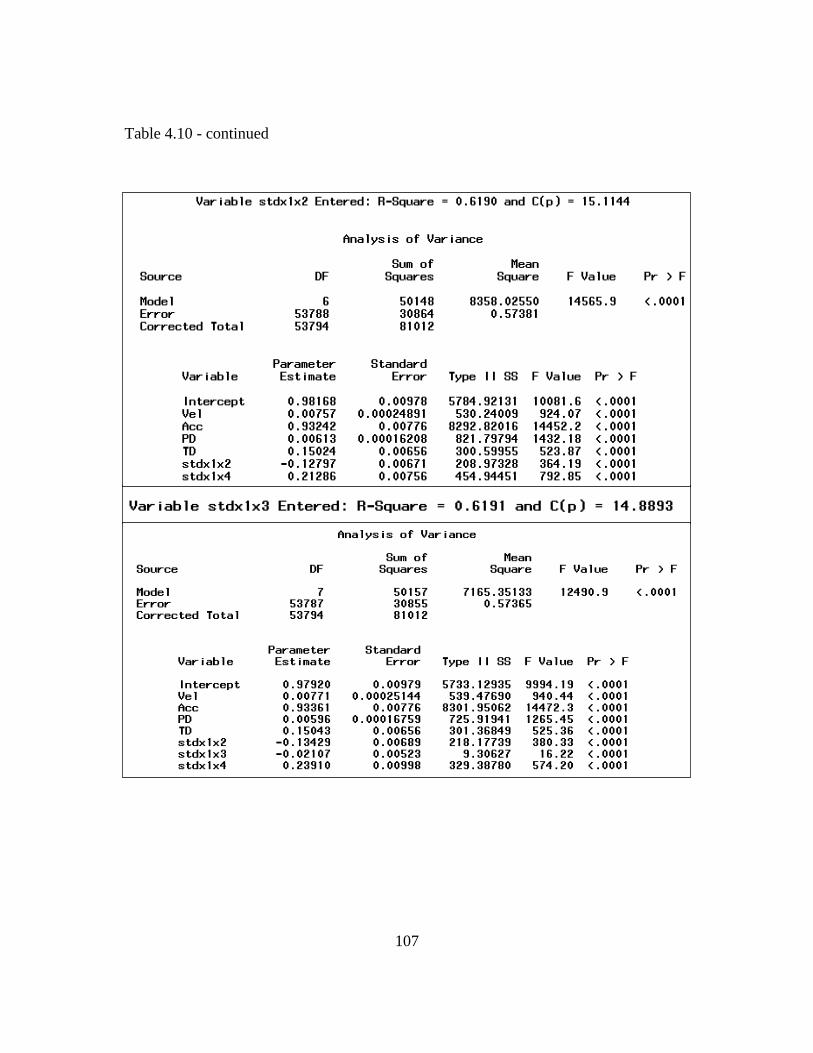
107
Table 4.10 - continued

108
Table 4.10 - continued
All variables left in the model are significant at the 0.05 level. No other variable met the
0.05 significance level for entry into the model.
Vel , Acc, PD, TD and stdx1x4, stdx2x4 (1st choice)
Vel, Acc, PD, TD, stdx1x2, stdx1x3 and stdx1x4 (2nd choice)
4.4.3 Backward Deletion
This is the simplest method among the three methods of variable selection. This
method starts with all the predictor variables in the model and removes those with
highest p-value greater than alpha critical (selected as 0.0500), one after the other. This
is because they are statistically insignificant. We ended up with the SAS program
selecting the model in Table 4.11 below.

109
Table 4.11 SAS Output for Backward Deletion Method
All variables left in the model are significant at the 0.0500 level.
In conclusion, the model with p-value<0.05 was selected.
Vel, Acc, Dec, PD, TD, stdx1x2 and stdx1x4, stdx2x4 (1st choice), if we
consider significance level at 0.1.
4.5 Potential “Best” Models
Summarizing the results obtained from the three methods of model search, we conclude
with the following best models.
Model A: Vel, Acc, PD, TD, stdx1x2 and stdx1x4 (1st choice)
Model B: Vel, Acc, PD, TD, stdx1x2, stdx1x3 and stdx1x4 (2nd choice)

110
4.5.1 Building the Regression Function
MODEL A
The regression function for Model A can be built from Table 4.12 below.
Table 4.12 SAS Output for Parameter Estimate for Model A
The regression function is:
41215421
^213.0128.0150.00.006923.0008.0982.0 xxxxxxxxy +−++++= Eqn. 4.3
Where
2COy =Λ
, (gram/sec)
x1 = Vehicle Velocity, V,(mi/hr)
x2 = Vehicle Acceleration, V,(mi/hr/sec)
x4 = Power Demand, PD, (mi2/hr2/sec)
x5 = Time of Day, TD,
From the correlation matrix in Table 4.13 below and the scatter plot matrix in
Figure 4.21 below, a strong correlation does not exist between the predictor variables.

111
Table 4.13 Correlation between Predictor Variables for Model A
Figure 4.21 Scatter Plot Matrix of Response and Predictor Variables

112
This model compared to the preliminary model shows an improvement in terms of
linear relationship between response variable and predictor variables and less
multicolinearity between predictor variables.
MODEL B
The regression function for Model B can be built from Table 4.14 below.
Table 4.14 SAS Output for Parameter Estimate for Model B
The regression function is:
Eqn. 4.4
Where
2COy =Λ
(grams/sec)
x1 = Vehicle Velocity, Vel,(mi/hr)
x2 = Vehicle Acceleration, Acc,(mi/hr/sec)
x3 = Vehicle Deceleration, Acc,(mi/hr/sec)
x4 = Power Demand, PD, (mi2/hr2/sec)
x5 = Time of Day, TD,
4131215421
^239.0021.0134.0150.00.006934.0008.0979.0 xxxxxxxxxxy +−−++++=

113
From the correlation matrix in Table 4.15 above and the scatter plot matrix in Figure
4.22 below, there is no high correlation or multicollinearity between predictor variables.
Table 4.15 Correlation between Predictor Variables for Model B
.

114
Figure 4.22 Scatter Plot Matrix of Response and Predictor Variables
The best model is selected from the two models above. To do this, various tests
including diagnostic, normality and constant variance tests for the two models are
conducted and make sure they satisfy them. The model that satisfies all the tests is
selected as the “best” overall model.

115
4.6 Verifying Model Assumptions
Table 4.16 below compares Model A with Model B
Table 4.16 Model Assumption Verification

116
Table 4.16- continued

117
4.7 Testing Goodness of Fit for Each Model
Analysis of Variance (ANOVA) and t-test tables from the SAS output will be
used to test the goodness of fit for each model:
Model A
Tables 4.17 and 4.18 show the SAS output of the ANOVA and T-test respectively, for
testing the goodness of fit for Model A.
Table 4.17 SAS ANOVA Output for Model A
Table 4.18 SAS T-test Output for Model A

118
Model B
Tables 4.19 and 4.20 show the SAS output of the ANOVA and T-test respectively, for
testing the goodness of fit for Model B.
Table 4.19 SAS ANOVA Output for Model B
Table 4.20 SAS T-test Output for Model B

119
From the ANOVA and t-test tables above:
The regression is significant for both models. This is because the p value (Pr>F)
is less than 10.0=α .
The coefficient of multiple determination ( )2R measures how well the
regression model fits the data set of CO2 emitted. ( ) ⇒== 6190.0/2 SSTOSSRR It can
be concluded that 62% of total variation in the mass emission rate of CO2 is explained
by the introduction of velocity, acceleration, power demand, time of day,
velocity*acceleration, and velocity*power demand in the model. The model appears to
fit well since the value is close to 1 ( )10 2 ≤≤ R . The remaining 38% is not accounted
for, or unexplained.
Similarly for model B, ( ) ⇒== 6191.0/2 SSTOSSRR It can be concluded that
62% of total variation in the mass emission rate of CO2 is explained by the introduction
of velocity, acceleration, power demand, time of day, (velocity*acceleration),
(velocity*deceleration) and (velocity*power demand) in the model. The model appears
to fit well since the value is close to 1 ( )10 2 ≤≤ R . The remaining 38% is not
accounted for, or unexplained. Several factors may have contributed to the unaccounted
portion of the dataset. These may include changes in weather conditions, road grade,
and air conditioning usage.
Model A: Passed all the tests except normality test. Normality test, however, is a
desired test, not a required one. In addition to that it is a simpler model to use compared
4.8 Summary of the Best Selected Model

120
to Model B. Moreover, Model A was selected as one of the 2 best models in two model
selection methods.
Model B: Passed all tests except the normality test, though the normality plot showed
that normality may be OK. Model B was selected as one of the 2 best models in one of
the three model selection methods.
Best model from a statistical point is model Model A.
Eqn. 4.3
4.9 Fitting the Preliminary Model for Highway Data
Table 4.21 Parameter Estimates
The result (SAS output) obtained is as follows:
From the SAS table in Table 4.21 above:
b0 = 0.97915
b1 = 0.02459
b2 = 0.57065
b3 = -0.21946
b4 = 0.01178
b5 = 0.03357
41215421
^213.0128.0150.00.006923.0008.0982.0 xxxxxxxxy +−++++=

121
So, the estimated regression function is:
54321
^034.0012.0219.0571.0.0250.9790 xxxxxy ++−++= Eqn. 4.5
4.10 Evaluating the Existing Model
The same evaluation procedure used for the arterial data is employed.
4.10.1 Preliminary Plots
The same procedure used in evaluating the arterial data is employed.
4.10.1.1 Response Variables vs. Predictor Variables and Predictor Variables vs. Predictor Variables
A similar scatter plot analysis between the mass emission rate of CO2 (response
variable) and the 5 different predictor variables are made with regards to the highway
data. The plots are shown in Figure 4.23 below.
Referring to Figure 4.23:
A correlation between “CO2” and “Vehicle Acceleration” is noticeable. A slight
linear trend shows a relationship between these two variables. This means that “Vehicle
Acceleration” can noticeably influence “CO2” emission rate and the positive slope of
the trend conveys that as “Vehicle Acceleration” increases, the mass emission rate of
“CO2” increases as well.
Plots do not show a high correlation between “CO2” with “Vehicle Velocity”
and “Time of Day”. This means that the two variables may slightly influence “CO2”,
although this is just a basic evaluation. Further tests and assessments will be conducted
in order to evaluate influences caused by the interaction terms as well.

122
“CO2” and “Power Demand” seem to be slightly correlated, which means this
predictor variable is influencing the response variable.
“Vehicle Acceleration” and “Power Demand” and “Vehicle Deceleration” and
“Power Demand”, on the other hand, look to be highly correlated and might lead to a
multicollinearity problem. This is the inter-correlation of independent variables and
occurs when two or more predictors are highly correlated. In the remaining plots, the
points seem to be fairly scattered and variables seem to be uncorrelated.
In some predictor vs. predictor plots as well as response vs. predictor plots,
some points appear to be potential x-outliers. Later some procedures will be conducted
to evaluate whether they should be thrown out.

123
Figure 4.23 Scatter Plots of Response and Predictor Variables
Similarly, Table 4.20 shows the correlation between the response variable and predictor
variables for the highway data.

124
Table 4.22 Correlation between Variables
From Table 4.22, we have the following preliminary conclusions:
ry1 = 0.26 indicates that CO2 and “Vehicle Velocity” are somewhat positively
correlated.
ry2 = 0.31 indicates that CO2 and “Vehicle Acceleration” are somewhat
positively correlated.
ry3 = 0.32 indicates that CO2 and “Vehicle Deceleration” are somewhat
positively correlated.
ry4 = 0.42 indicates that CO2 and “Power Demand” are somewhat positively
correlated.
ry5 = -0.04 indicates that there is little correlation between CO2 and “Time of
Day”.
r12 = -0.27 indicates that “Vehicle Velocity” and “Vehicle Acceleration” are
somewhat negatively correlated.

125
r13 = 0.21 indicates that “Vehicle Velocity” and “Vehicle Deceleration” are
somewhat positively correlated.
r14 = 0.001 indicates that there is little correlation between “Vehicle Velocity”
and “Power Demand”.
r15 = -0.22 indicates that “Vehicle Velocity” and “Time of Day” are somewhat
negatively correlated.
r23 = 0.25 indicates that “Vehicle Acceleration” and “Vehicle Deceleration” are
somewhat positively correlated.
r24 = 0.65 indicates that “Vehicle Acceleration” and “Power Demand” are
positively highly correlated.
r25 = -0.06 indicates that there is little correlation between “Vehicle
Acceleration” and “Time of Day”.
r34 = 0.80 indicates that there is little correlation between “Vehicle
Deceleration” and “Power Demand” are positively highly correlated.
r35 = -0.07 indicates that there is little correlation between “Vehicle
Deceleration” and “Time of Day”.
r45 = -0.01 indicates that there is little correlation between “Power Demand” and
“Time of Day”.
From the numbers presented in Table 4.22, it can be deduced that a correlation
exists between predictor variables in at least two cases, “Vehicle Acceleration” and
“Power Demand” and “Vehicle Deceleration” and “Power Demand”. This may be a

126
potential multicollinearity problem. Further tests will help in making a final decision on
the multicolinearity issue.
4.10.2 Residual Plots for Highway Data
4.10.2.1 Residuals vs. ŷi
From Figure 4.24 below, we cannot detect any funnel. The plot does not show
any curvilinear shape but a couple of potential outliers can be observed. So far what can
be concluded is that the “constant variance” assumption is probably OK. Further tests
will be conducted to verify the conclusion from this plot.
Figure 4.24 Residual vs. Predicted Value of CO2
4.10.2.2 Residuals (e) vs. Predictor Variables
In this series of plots shown in Figure 4.25, curvature cannot be detected.
Curvature would indicate violation of the assumed model form, which is currently a
linear equation. There are also some possible outliers.

127
Figure 4.25 Residual vs. Predictor Variables
4.10.2.3 Residuals vs. Interaction Terms
Basically, what we are looking for in Figure 4.26 plots below is a trend between
the residuals and any interaction terms. If a trend is seen, we can suggest adding the
associated interaction terms to the model.

128
Figure 4.26 Residuals vs. Interaction Terms
As shown in Figure 4.26 above, there is not a strong trend among the plots.
There might be a slight trend between residuals and x2x5, x2x4 and x3x4, but at this
point we are not suggesting that any interaction terms should be added.
4.10.3 Normal Probability Plot of ei’s
The normality plot shown in Figure 4.27 does not deviate much from a straight-
line. There is slight indication of a longer right tail and a shorter left tail than the normal
distribution. However, on the strength of the straightness of the plot, normality seems

129
generally OK. Further tests will be conducted and a final decision on normality will be
made later.
Figure 4.27 Normal Probability Plot
4.10.4 Time Series Plot
The time series plot in Figure 4.28 below shows a slight upward trend, which
might indicate serial correlation between the observations.

130
Figure 4.28 Time Series Plot
4.11 Verifying the Model Assumptions
In this section, tests and diagnostics are presented to further verify model
assumptions that have been assessed visually from the plots.
4.11.1 Test for Constant Variance (Modified Levene Test)
A further test is conducted to confirm the initial assumption from the plots that
the “constant variance” assumption is OK. Figure 4.29 and Table 4.21 are considered in
this test.
Ho: Variances are equal
Test: vs.
H1: Variances are not equal

131
Figure 4.29 Residual vs. Predicted Value of CO2
As discussed previously, we concluded from the residual plots that the “constant
variance” assumption is OK. The Modified Levene Test will be used to confirm this
conclusion. This test does not depend on the normality of the error terms. To conduct
this test, we divide the data into two groups of about the same number of observations.
The cutoff line on ŷ i will fall around value “2.8”. This line is illustrated on the residual
vs. ŷi plot in Figure 4.29.
Table 4.23 SAS Output for Testing Constant Variance

132
Table 4.23 shows the result of conducting the test using SAS and using 2 groups
with about the same number of observations in each of them. Assuming α=0.1 for the
confidence level, the p-value for the test turns out to be greater than α=0.1. Thus:
P-value=0.3579>0.1=α ⇒ we fail to reject H0.
This leads us to conclude that the assumption of “constant variance” is OK.
4.11.2 Test for Normality
Further testing is conducted to support the initial assumption that normality is
generally OK, as follows:
H0: Normality is OK
Test: Vs.
H1: Normality is violated
The following table is obtained from the SAS output.
Table 4.24 Normality Test from SAS Output
We need to find ( )nc ,α in order to compare it with the correlation value
^ρ (from the SAS output) in Table 4.22. With 10.0=α , we have
989.0)55342,10.0( === nc α ; this implies ⇒>= 989.099396.0^ρ fail to reject Ho.
Hence normality is OK.

133
4.11.3 Outlier Diagnostic
Y-Outlier: Bonferroni test cutoff: t(1-α /2n, n-p-1) = t(1-0.10/(2*55342));
55342-6-1) = t(0.999999, 55335) = 3.291. When compared with the Rstudent values in
APPENDIX A, the values are less than 3.291; we then conclude that there are no y –
outliers.
X-Outlier: Leverage values (hii) are utilized to check whether x-outliers exist or
not. The hii values (APPENDIX A) are compared with the valuenp2 = 2(6)/55342 =
0.0002. If any hii value from APPENDIX A>0.0002, then it can be concluded that x-
outliers exist. We can detect a few observations greater than 0.0002, but we do not
have any reason for deleting them; hence, we leave them in the dataset and continue
with the analysis.
Influence on the Fitted Values: DFFITS
The DFFITS values for any outliers (APPENDIX A) are compared with the
valuenp2 =
5534262 = 0.021. If the DFFITS value for an outlier > 0.021, then that
outlier has high influence on the estimated regression equation and fitted values. From
APPENDIX A, there are a few DFFITS values higher than np2 = 0.021.
Cut-off DFBETA (influence on the individual LSEs)
The DFBETA values (APPENDIX A) are compared with the value
5534222
=n
= 0.009. If the DFBETA value for an outlier >0.009, then that outlier

134
has high influence on the least square estimates. From the value of DFBETA in
APPENDIX A, a few observations have higher values than 0.009.
4.11.4 Multicollinearity - Variance Inflation
From the assessment of the predictor variables using the Correlation Matrix, a
potential multicollinearity problem was discovered. Table 4.21, repeated here for
convenience, shows only one number slightly greater than “5” under the “Variance
Inflation” column. Therefore, up to this point, multicollinearity may not be a problem.
Table 4.21 SAS Output for Assessing Variance Inflation
4.11.5 Assessing Partial Regression Plots for Highway Data
Following the same procedure as in the arterial data plots, partial regression
graphs for highway data are plotted and analyzed. The resulting plots are shown in
Figure 4.20-4.39. Trends are difficult to see on both Figures 4.30-4.39 and 4.340, hence,
all terms will be added and the model selection procedures will be used to try to identify
any helpful interaction terms.

135
Figure 4.30 Residual e(Y/x1x2x3x4x5) vs. Residual e(x1x2/x1x2x3x4x5)
Figure 4.31 Residual e(Y/x1x2x3x4x5) vs. Residual e(x1x3/x1x2x3x4x5)

136
Figure 4.32 Residual e(Y/x1x2x3x4x5) vs. Residual e(x1x4/x1x2x3x4x5)
Figure 4.33 Residual e(Y/x1x2x3x4x5) vs. Residual e(x1x5/x1x2x3x4x5)

137
Figure 4.34 Residual e(Y/x1x2x3x4x5) vs. Residual e(x2x3/x1x2x3x4x5)
Figure 4.35 Residual e(Y/x1x2x3x4x5) vs. Residual e(x2x4/x1x2x3x4x5)

138
Figure 4.36 Residual e(Y/x1x2x3x4x5) vs. Residual e(x2x5/x1x2x3x4x5)
Figure 4.37 Residual e(Y/x1x2x3x4x5) vs. Residual e(x3x4/x1x2x3x4x5)

139
Figure 4.38 Residual e(Y/x1x2x3x4x5) vs. Residual e(x3x5/x1x2x3x4x5)
Figure 4.39 Residual e(Y/x1x2x3x4x5) vs. Residual e(x4x5/x1x2x3x4x5)

140
Table 4.25 Correlation between Interaction Terms and Predictors
Table 4.26 Correlation between Interaction Terms and Predictors

141
Table 4.27 Correlation between Standardized Interaction Terms and Predictors
Table 4.28 Correlation between Standardized Interaction Terms and Predictors

142
Figure 4.40 Scatter Plots of Residual vs. Standardized Interaction Terms
4.12 Model Selection (Best Potential Model) for Highway Data
The same selection process used for the arterial data is applied to the highway data.
4.12.1 Best Subset Selection
The result from the SAS program is shown in Table 4.29 below.

143
Table 4.29 SAS Output for the Best Subset Method
In conclusion, using the idea of R2 leveling off and Cp close to P (the number of
parameters), the following two best models were selected.
Vel , Acc, PD, TD, stdx1x3 and stdx2x4 ( 1st choice)

144
Vel , PD, TD, stdx1x2, stdx2x3 and stdx2x4 (2nd choice)
4.12.2 Stepwise Regression
The result from the SAS program is shown in Table 4.30 below.
Table 4.30 SAS Output for Stepwise Regression Method

145
Table 4.30-continued

146
Table 4.30-continued
All variables left in the model are significant at the 0.05 level. No other variable
met the 0.05 significance level for entry into the model.
Vel, PD, TD, stdx1x2, stdx2x3 and stdx2x4 (1st choice)
Vel , PD, stdx1x2, stdx2x3 and stdx2x4 (2nd choice)

147
4.12.3 Backward Deletion
We ended up with the SAS program selecting the model in Table 4.31 below.
Table 4.31 SAS Output for Backward Deletion Method

148
All variables left in the model are significant at the 0.0500 level.
In conclusion, the model with p-value<0.05 was selected.
Vel, Acc, Dec, PD, TD, stdx1x2 and stdx2x4 (best choice), if we consider
significance level at 0.1.
4.13 Potential “Best” Models
Summarizing the results obtained from the three methods of model search, we
conclude with the following best models.
Model A: Vel, PD, TD, stdx1x2, stdx2x3 and stdx2x4 (1st choice)
Model B: Vel, Acc, PD, TD, stdx1x3 and stdx2x4 (2nd choice)
4.13.1 Building the Regression Function for the Highway Data
MODEL A
The regression function for Model A can be built from Table 4.32 below.
Table 4.32 SAS Output for Parameter Estimate for Model A
The regression function is:
Eqn.4.6
423221541
^013.0225.0022.0036.00.014025.0034.1 xxxxxxxxxy ++−+++=

149
Where
2COy =Λ
, (gram/sec)
x1 = Vehicle Velocity, V,(mi/hr)
x2 = Vehicle Acceleration, Acc,(mi/hr/sec)
x3 = Vehicle Deceleration, Dec,(mi/hr/sec)
x4 = Power Demand, PD, (mi2/hr2/sec)
x5 = Time of Day, TD, (1 for peak, 0 for offpeak)
From the correlation matrix in Table 4.33 below and the scatter plot matrix in Figure
4.41 below, a strong correlation does not exist between the predictor variables.
Table 4.33 Correlation between Predictor Variables for Model A
.

150
Figure 4.41 Scatter Plot Matrix of Response and Predictor Variables
This model compared to the preliminary model shows an improvement in terms
of linear relationship between response variable and predictor variables and less
multicolinearity between predictor variables.

151
MODEL B
The regression function for Model B can be built from Table 4.34 below.
Table 4.34 SAS Output for Parameter Estimate for Model B
The regression function is:
42315421
^013.0026.0036.00.009633.0025.0978.0 xxxxxxxxy ++++++= Eqn.4.7
Where
2COy =Λ
(gram/sec)
x1 = Vehicle Velocity, V,(mi/hr)
x2 = Vehicle Acceleration, Acc.(mi/hr/sec)
x3 = Vehicle Deceleration, Dec.(mi/hr/sec)
x4 = Power Demand, PD, (mi2/hr2/sec)
x5 = Time of Day, TD,
From the correlation matrix in Table 4.32 above and the scatter plot matrix in
Figure 4.42 below, there is no high correlation or multicollinearity between predictor
variables.

152
Table 4.35 Correlation between Predictor Variables for Model B
Figure 4.42 Scatter Plot Matrix of Response and Predictor Variables

153
The best model is selected from the two models above. To do this, various tests
including diagnostic, normality and constant variance tests for the two models are
conducted and make sure they satisfy them. The model that satisfies all the tests is
selected as the “best” overall model.
4.14 Verifying Model Assumptions
Table 4.36 below compares Model A with model B
Table 4.36 Model Assumption Verification

154
Table 4.36-continued

155
4.15 Testing Goodness of Fit for Each Model
Analysis of Variance (ANOVA) and t-test tables from the SAS output will be
used to test the goodness of fit for each model:
Model A
Tables 4.37 and 4.38 show the SAS output of the ANOVA and T-test,
respectively, for testing the goodness of fit for Model A.
Table 4.37 SAS ANOVA Output for Model A
Table 4.38 SAS T-test Output for Model A

156
Model B
Tables 4.39 and 4.40 show the SAS output of the ANOVA and T-test,
respectively, for testing the goodness of fit for Model B.
Table 4.39 SAS ANOVA Output for Model B
Table 4.40 SAS T-test Output for Model B
From the ANOVA and t-test tables above:

157
The regression is significant for both models. This is because the p value
(Pr>F) is less than 10.0=α .
( ) ⇒== 2675.0/2 SSTOSSRR It can be concluded that 27% of total
variation in the mass emission rate of CO2 is explained by the introduction of velocity,
power demand, time of day, (velocity*acceleration), (acceleration*deceleration) and
(acceleration*power demand) in the model. The model does not appear to fit that well
since the value is so low ( )10 2 ≤≤ R . The remaining 73% is not accounted for, or
unexplained.
Similarly for model B, ( ) ⇒== 2675.0/2 SSTOSSRR It can be concluded that
27% of total variation in the mass emission rate of CO2 is explained by the introduction
of velocity, acceleration, power demand, time of day, (acceleration*deceleration) and
(acceleration*power demand) in the model. The model does not appear to fit that well
since the value is so low ( )10 2 ≤≤ R . The remaining 73% is not accounted for, or
unexplained.
Similarly, factors such as changes in weather conditions, road grade, and air
conditioning usage may have contributed to the unaccounted portion of the dataset.
4.16 Summary of the Best Selected Model
Model A: Passed all the tests and in addition to that it is a simpler model to use
compared to Model B. Moreover, Model A was selected as one of the 2 best models in
two model selection methods.

158
Model B: Passed all tests that normality is OK. Model B was selected as one of
the 2 best models in two of the three model selection methods.
From a statistical point of view, the best model is Model A.
423221541
^013.0225.0022.0036.00.014025.0034.1 xxxxxxxxxy ++−+++=
Eqn.4.6
(i) They are simple models.
4.17 Selection of Best Model, Including Factors Other Than Statistical
Statistical factors, like R2 values and Cp values, are only one set of factors to
consider in choosing a model. Other factors include complexity of use, whether it is
consistent with theory, and whether it gives realistic emission estimates. These
additional factors are considered in this section
4.17.1 Other Models with High R2 values
SAS output includes only the top two models in each category (number of
terms),e.g. the top two models with two terms, the top two models with three terms, etc.
However, in this research, the R2 values for the top two models in each category were
only slightly higher than models ranked lower. This section presents some of the lower
ranked models, which had comparable R2 values.
Eqns.4.8 - Eqn. 4.10 (arterial models) and Eqns.4.11 - Eqn. 4.13 (highway
models) were selected from the other SAS output models for the following reasons:
(ii) The independent variables present are velocity, acceleration and
velocity* acceleration. These variables are representative of variables
found in other fuel consumption models such as Eqn.2.5,

159
and in practice, influence fuel consumption rates as well as exhaust
emissions rate.
4.17.1.1 Arterial Models
0.006PD982.0010.0007.1^
+++= AccVely R2= 0.6094 Eqn. 4.8
Acc*0.208Vel172.1011.0867.0^
+++= AccVely R2=0.6050 Eqn.4.9
AccVely 145.1011.0902.0^
++= R2 = 0.5967 Eqn.4.10
PDVelAccVelTDPDAccVely *213.0*128.0150.00.006923.0008.0982.0^
+−++++=
R2= 0.6190 Eqn.4.3
4.17.1.2 Highway Models
R2 = 0.2646 Eqn. 4.11
R2 = 0.2250 Eqn. 4.12
R2= 0.2650 Eqn. 4.13
R2= 0.2675 Eqn.4.6
0.009PD702.0024.0071.1^
+++= AccVely
AccVely 318.1028.0707.0^
++=
Acc*0.060Vel538.1026.0765.0^
+++= AccVely
4
^*013.0*225.0*022.0036.00.014025.0034.1 PDAccDecAcAccVelTDPDVely ++−+++=

160
4.17.2 Estimation of CO2 Emissions from considered Arterial and Highway Models
This section presents case studies of CO2 emissions calculated using different
models.
Table 4.41 CO2 Emissions Using Actual Values in Arterial Models, Acceleration=0 (Cruise Mode)
CO2 emissions (gram/sec)
Acc=0
5mi/hr 10mi/hr 15mi/hr 20mi/hr 25mi/hr 30mi/hr 35mi/hr 40mi/hr
Eqn.4.8 1.06 1.11 1.16 1.21 1.26 1.31 1.36 1.41
Eqn.4.9 0.92 0.98 1.03 1.09 1.14 1.20 1.25 1.31
Eqn.4.10 0.96 1.01 1.07 1.12 1.18 1.23 1.29 1.34
Eqn.4.3 1.10 1.14 1.18 1.22 1.26 1.30 1.34 1.38
Table 4.42 CO2 Emissions Using Actual Values in Arterial Models, Acceleration=1mi/hr/sec
CO2 emissions (gram/sec)
Acc=1mi/hr/sec
5mi/hr 10mi/hr 15mi/hr 20mi/hr 25mi/hr 30mi/hr 35mi/hr 40mi/hr
Eqn.4.8 2.07 2.15 2.23 2.31 2.39 2.47 2.55 2.63
Eqn.4.9 3.13 4.23 5.32 6.42 7.51 8.61 9.70 10.80
Eqn.4.10 2.10 2.16 2.21 2.27 2.32 2.38 2.43 2.49
Eqn.4.3 6.74 22.15 48.20 84.91 132.26 190.27 258.92 338.23

161
Table 4.43 CO2 Emissions Using Actual Values in Arterial Models, Acceleration=2mi/hr/sec
CO2 emissions (gram/sec)
Acc=2mi/hr/sec
5mi/hr 10mi/hr 15mi/hr 20mi/hr 25mi/hr 30mi/hr 35mi/hr 40mi/hr
Eqn.4.8 3.08 3.19 3.30 3.41 3.52 3.63 3.74 3.85
Eqn.4.9 5.35 7.48 9.62 11.75 13.89 16.02 18.16 20.29
Eqn.4.10 3.25 3.30 3.36 3.41 3.47 3.52 3.58 3.63
Eqn.4.3 12.39 43.16 95.23 168.60 263.27 379.24 516.51 675.08
Table 4.44 CO2 Emissions Using Actual Values in Highway Models, Acceleration=0 (Cruise Mode)
CO2 emissions (gram/sec)
Acc=0
45mi/hr 50mi/hr 55mi/hr 60mi/hr 65mi/hr 70mi/hr 75mi/hr 80mi/hr
Eqn.4.11 2.15 2.27 2.39 2.51 2.63 2.75 2.87 2.99
Eqn.4.12 1.97 2.11 2.25 2.39 2.53 2.67 2.81 2.95
Eqn.4.6 2.18 2.30 2.43 2.55 2.68 2.80 2.93 3.05
Eqn.4.13 1.94 2.07 2.20 2.33 2.46 2.59 2.72 2.85

162
Table 4.45 CO2 Emissions Using Actual Values in Highway Models, Acceleration=1mi/hr/sec
CO2 emissions (gram/sec)
Acc=1mi/hr/sec
45mi/hr 50mi/hr 55mi/hr 60mi/hr 65mi/hr 70mi/hr 75mi/hr 80mi/hr
Eqn.4.11 3.26 3.42 3.59 3.75 3.92 4.08 4.25 4.41
Eqn.4.12 3.29 3.43 3.57 3.71 3.85 3.99 4.13 4.27
Eqn.4.6 2.15 2.30 2.45 2.60 2.75 2.90 3.05 3.20
Eqn.4.13 6.17 6.60 7.03 7.46 7.89 8.32 8.75 9.18
Table 4.46 CO2 Emissions Using Actual Values in Highway Models, Acceleration=2mi/hr/sec
CO2 emissions (gram/sec)
Acc=2mi/hr/sec
45mi/hr 50mi/hr 55mi/hr 60mi/hr 65mi/hr 70mi/hr 75mi/hr 80mi/hr
Eqn.4.11 4.37 4.58 4.79 5.00 5.21 5.42 5.63 5.84
Eqn.4.12 4.60 4.74 4.88 5.02 5.16 5.30 5.44 5.58
Eqn.4.6 3.29 3.59 3.90 4.20 4.51 4.81 5.12 5.42
Eqn.4.13 10.41 11.14 11.87 12.60 13.33 14.06 14.79 15.52
The trends in Tables 4.41-4.46 are what would be expected, in that emissions
increase across each table as velocity increases. This is due to the fact that an increase
in speed causes more fuel to be burned, correspondingly producing more tailpipe

163
emissions including carbon dioxide emissions. In addition, emissions predicted by a
given equation for a given velocity increase. An increase in the change in velocity per
unit time, acceleration, puts more load on the engine and requires more fuel to be
burned producing more carbon dioxide emissions. For the cruise cases (acceleration =
0), emissions predicted by all 4 models at a given speed are very similar.
Emissions estimated for acceleration = 1 mi/hr/sec and 2 mi/hr/sec using Eq. 4.3
are very high compared with the estimates given by the other equations. Eq. 4.3 likely
overestimates emissions at higher speeds, for acceleration = 1 mi/hr/sec and 2 mi/hr/sec,
according to a check run using the carbon equivalent of gasoline published in the Code
of Federal Regulations (40 CFR 600.113) and used by the Environmental Protection
Agency in fuel economy calculations.
As speeds increase from 40 mi/hr arterial to 45 mi/hr highway, discontinuities
exist between Tables 4.42 (arterial) and 4.45 (highway), and Tables 4.43 (arterial), and
4.46(highway). In most cases, emissions calculated by a given equation for 45 mph
highway are greater than emissions estimated for 40 mph by the corresponding arterial
equation. The discontinuity issue may be due to the fact that the highway model was
built with velocity values less than 45mile/hr inclusive. The discontinuities do not occur
for the cruise cases (acceleration = 0).

164
4.17.3 Final Choice of Models
From a statistical stand point, the models selected were Eqn. 4.3 (for arterial)
and Eqn.4.6 (for highway), taking into account the model selection process. Factors
such as R2, Adjusted R2, and Cp closer to P were considered. As explained earlier, the
model with the highest R2 value, highest adjusted R2 value and Cp closest to P was
selected as the best model from a statistical viewpoint, after passing all the models’
assumption tests. Eqn. 4.3 & Eqn. 4.6 satisfied all these conditions and hence ended up
as the selected models.
However, these models contain a lot of variables and interaction terms, which
makes them complex. In addition, the negative coefficient in front of the interaction
term, velocity* acceleration, which occurs in both equations, is not consistent with
theory and practice. Theoretical models developed for estimating fuel consumption or
emissions show positive coefficient values for velocity and acceleration variables,
which indicates that emissions would increase with increase in these variables. This is
consistent with what real world situations depict: as velocity and acceleration increase,
fuel consumption and emissions also increase. In most emissions and fuel consumption
models, such as Eqn. 4.13 below, velocity and acceleration are two important variables
responsible for vehicle emissions increase.
Therefore, a model containing velocity acceleration and velocity*acceleration with all
the terms positive will be plausible. Further the model should be simple.
Table 4.47 summarizes advantages and disadvantages associated with the
various arterial models.

165
Table 4.47 Advantages and Disadvantages Associated with the Arterial Models
Equation Number of Independent Variables/Variable Groups
R2 Simple or Complex?
Fuel Economy basis?
Emission Estimates Realistic?
4.8 3 0.6094 Simple No Don’t vary much with speed
4.9 3 0.6050 Simple Yes Seem reasonable
4.10 2 0.5968 Simple Yes Don’t vary much with speed
4.3 6 0.6190 Complex No, and interaction term has negative coefficient
Likely too high
For the arterial models, Eqn.4.3 (R2=0.6190) has a higher R2 value, but it likely
over predicted emissions. In addition, due to the greater number of independent
variables, it is more complex to use. Eqn.4.9 (R2 = 0.6050) has about the same R2 value
as Eqn. 4.3, contains fewer variables, and has a basis in fuel economy models. In Tables
4.41 and 4.42, Eq. 4.8 and 4.10 do not predict much of an emissions increase with
velocity, as would be expected. Eqn.4. 9 was hence selected as the final arterial model.

166
Table 4.48 summarizes advantages and disadvantages associated with the
various highway models.
Table 4.48 Advantages and Disadvantages Associated with the Highway Models
Equation Number of
Independent
Variables/Variable
Groups
R2 Simple or
Complex?
Fuel
Economy
basis?
Emission
Estimates
Realistic?
4.11 3 0.2646 Simple No Yes
4.12 2 0.2250 Simple Yes Yes
4.6 6 0.2675 Complex No Yes
4.13 3 0.2650 Simple Yes Yes
Of the highway models, Eqn.4.6, due to the greater number of independent
variables, is more complex to use. Eqn. 4.13 is a simpler model containing velocity,
acceleration and velocity*acceleration, which are important independent variables
present in most fuel consumption models such as the one in Eqn. 2.5. From Table 4.48,
Eqn. 4.11 does not have a basis in fuel consumption models while the R2 value of Eqn.
4.12 is lower. Therefore Eqn. 4.13 was selected as the final highway model.
Eqn.4.9 & Eqn. 4.13, which are much simpler and contains variables such as
velocity and acceleration that are representative of vehicle emissions estimation, are
selected as the final models for the arterial and highway datasets, respectively. These
models have R2 and adjusted R2values almost as high as the models previously selected

167
purely on statistical rationale, in addition, the coefficients of all variables and
interaction terms are positive.
Similarly, it should be noted that, the chosen arterial model can only be used
over velocity ranges of 0 to 54 mile per hour, acceleration ranges of 0 to 4.9 mile per
hour per second, and power demand ranges of 0 to 119 mi2per hr2 per sec. These ranges
represent the range of values used in developing the model.
61% of total variation in the mass emission rate of CO2 is explained by the
chosen arterial model.
The remaining 39%, which was not accounted for in the model may be due to
factors such as road grade, weather conditions, air conditioning usage, tire pressure
(needed to be checked and made sure the amount of air in tire is consistent throughout
the data collection period), road surface conditions and total vehicle weight.
Similarly, the chosen highway model can only be used over velocity ranges of 0
to 85 mile per hour, acceleration ranges of 0 to 4.5 mile per hour per second, and power
demand ranges of 0 to 315 mi2per hr2 per sec. These ranges represent the range of
dataset used in developing the model.
27% of total variation in the mass emission rate of CO2 is explained by the
highway model.
The remaining 73% is not accounted for, or unexplained. This unexplained part of the
R2 may be due to factors such as road grade, weather conditions, air conditioning usage,
tire pressure (needed to be checked and made sure the amount of air in tire is consistent
throughout the data collection period), road surface conditions and total vehicle weight

168
(which may have changed due to different drivers and passengers). Further, it may be
due to the fact that the data used in developing the highway model contained speed data
that is below 45miles per hour, which is representative of speeds found on an arterial
facility, and may have represented anomalous conditions for the highway. Future
research using freeway data should exclude velocity data less than 45 miles per hour.
The coefficients of both the velocity and the acceleration terms for the highway
model are higher than for the arterial model. This is an indication that, on the highway
facility, the changes in velocity and acceleration would produce higher CO2 emissions
compared with an arterial facility.
Unlike MOBILE 6.2 which contain vehicle velocity as the only traffic variable,
the chosen arterial and highway models are functions of both velocity and acceleration
and could better explain the dynamics associated with driving.
The models can be coupled with a micro scale traffic model to evaluate
emissions impact of transportation system measures such as:
• traffic signal coordination
• speed limit reductions
• extended idling reductions
• bottleneck removal.

169
CHAPTER 5
CONCLUSIONS AND RECOMMENDATIONS
1. Arterial model:
5.1 Conclusions
A Multiple Linear Regression method which incorporates Statistical Analysis
System (SAS) software was used to develop CO2 emissions models for a light duty
gasoline vehicle. This statistical method was used as a tool to identify useful
explanatory variables.
5.1.1 Final Carbon Dioxide (CO2) Models
The models to estimate carbon dioxide emissions on a second-by-second basis
are:
2. Highway model:
Where
2COy =Λ
(grams/sec),
Vel = Vehicle Velocity,(mi/hr),
Acc*0.208Vel172.1011.0867.0^
+++= AccVely
Acc*0.060Vel538.1026.0765.0^
+++= AccVely

170
Acc= Vehicle Acceleration,(mi/hr/sec),
Given the large set of second by second data collected, the number of variables
examined and the surrogate nature of the variables, the overall R2 value of 0.61 for CO2
demonstrated a strong model fit to the arterial dataset, whereas the overall R2 value of
0.27 for CO2 demonstrated a weak model fit to the highway dataset. However, all final
model variables are statistically significant as indicated by the P-values from the SAS
output in the tables.
Further, unlike other models that predict vehicle emissions with velocity as the
sole vehicle activity variable responsible for higher emissions, these models developed
contain an additional variable, acceleration, which accounts for the dynamics involved
in vehicle activity.
• On – board emissions measurement methods should be used in future studies to
improve knowledge of real-world on-road tailpipe emissions.
5.2 Recommendations
• On-road measurement studies should be carefully designed, taking into account
well-defined study objectives.
• Variability and uncertainty should be accounted for in the study design and
when making inferences based upon measured data. That is, driving behavior during
data collection should be as consistent as possible; in addition, variation in road grade,
air conditioning usage and weather conditions under which data is collected should be

171
minimized. The impact, however, of accounting for these variability and uncertainty
could lead to an improvement of the coefficient of determination (R2).
• UTA and others should use on-road emissions data to aid in the design and
evaluation of transportation control measures (TCMs) and transportation
implementation programs (TIPs).
• Further research can be conducted by developing CO and HC models, as well as
testing diesel vehicles.

172
APPENDIX A
ARTERIAL SAS OUTPUT FOR X & Y OUTLIERS DETERMINATION

173

174

175

176

177

178

179
APPENDIX B
HIGHWAY SAS OUTPUT FOR X & Y OUTLIERS DETERMINATION

180

181

182

183

184

185

186
REFERENCES
1. H. Christopher Frey; Nagui M. Rouphil; A. Unal; James D. Colyar; “Measurement of
On- Road Tailpipe CO, NO, and Hydrocarbon Emissions using a portable instrument”;
Journal of Air and Waste Management Association, June 24-28, 2001.
2. Nagui M. Rouphil; H. Christopher Frey; James D. Colyar; Alper Unal; “Vehicle
Emissions and traffic Measures: Exploratory Analysis of Field Observations at
Signalized Arterials”; Annual meeting of the Transportation research Board, January 7-
11, 2001.
3. U.S Environmental Protection Agency home page. See
http://www.epa.gov/otaq/invntory/overview/definitions.htm, (accessed December,
2006).
4. Yi Grace Qi; Hualiang Harry Teng; and Lei Yu; “Microscale Emissions Models
Incorporating Acceleration and Deceleration”; Journal of Transportation Engineering
at ASCE, May/June 2004.
5. Rakesh B. Singh; James J. Sloan; “Development and Application of a Microscale
Emission Factor Model (MicroFac) for Mobile Source Emissions”; Annual Emission
Inventory Conference, Las Vegas, April 11-15, 2005.

187
6. Remote Sensing: A Supplemental tool for Vehicle Emission Control; U.S
Environmental Protection Agency Office of Mobile Sources, August 1993.
7. City of Albuquerque; Remote Sensing: Vehicle Pollution Management.
http://www.cabq.gov/aircare/rst.html (accessed September 14, 2007).
8. Melanie Sattler; Transportation and Air quality lecture notes fall 2005.
9. Melanie Sattler, Air pollution Dispersion modeling lecture notes, fall 2005.
10. Randall Guensler; Data Needs for Evolving Motor Vehicle Emission Modeling
Approaches; Georgia Tech., Atlanta, 1993.
11. A. Unal, H; Christopher Frey; Nagui M. Rouphail; James D. Colyer; Hot Spot
Analysis of Real World Vehicle Emissions based upon a Portable On-board
Measurement System; North Carolina, Raleigh, 2001.
12. John Neter; Michael H. Kutner; Christopher J. Nachtsheim; Williams Li; Applied
Linear Statistical Models; Fifth edition, 1996.

188
13. Shauna L. Hallmark, Randall Guensler, and John D. Leonard II, Stopline
Distributions of Speed and Acceleration for Signalized Intersections, School of Civil
and Environmental Engineering, Georgia Tech., Atlanta, Georgia, 30332, 1998.
14. U.S Department of Transportation and Federal Highway Administration; Air
Quality and Transportation; See http://www.tfhrc.gov/pubrds/03jul/10.htm (accessed
January, 2007).
15. Robert Jourmard; Peter Jost; John Hickman; Dieter Hassel; Hot Passenger Car
Emissions Modeling as a Function of Instantaneous Speed and Acceleration; 1994.
16. Environmental Protection Agency, Clean Air Act,
http://www.epa.gov/oar/oaqps/pegcaa/pegcaa02.html (accessed January 2007).
17. Environmental Protection Agency; Green Book-Criteria Pollutant;,
http://www.epa.gov/oar/oaqps/greenbk/o3co.htm (accessed September, 2007).
18. Alper Unal; Nagui M. Rouphail; H. Christopher Frey; Effect of Arterial
Signalization and Level of Service on Measured Vehicle Emissions; Transportation
Research record 1842 paper No. 03-2884.
19. Steven H. Cadle; Robert A. Gorse; Timothy C. Belian; Douglas R. Lawson;

189
“Real-World Vehicle Emission: A Summary of the Eighth Coordinating Research
Council On-Road Vehicle Emissions Workshop”; Journal of the Air & Waste
Management Association; March 1999.
21. Dr. Christopher Frey; Dr. Nagui Rouphail; Alper Unal; James Colyar; Emissions
reduction Through Better Traffic Management: An Empirical Evaluation Based Upon
On-Road Measurements; North Carolina State University: North Carolina, Raleigh, NC
27695, December 2001.
22. Ignatus Fomunung; Simon Washington; Randall Guensler; Comparison of Measure
and Mobile 5a predictions Using Laboratory Measurements of Vehicle Emission;
Transportation Planning and Air Quality; Georgia Institute of Technology: Atlanta,
Georgia, 1999.
23. Horiba Instruments Inc.; On-board Emission Measurement System, OBS-1000
Instruction Manual; 2003.
24. Gary R. McGaughey; Nimish R. Desai; David T. Allen; Robert L. Seila; William A.
Lonneman; Matthew P. Fraser; Robert A. Harle;, Alison K. Pollack; Jason M. Ivy;
James H. Price; Analysis of motor vehicle emissions in a Houston tunnel during the
Texas Air Quality Study; Atmospheric Environment 38, 2004.

190
25. Roger Westerholm; Karl-Erik Egeback; Exhaust Emissions from Light-duty and
Heavy-duty Vehicles: Chemical Composition, Impact of Exhaust after Treatment, and
Fuel Parameters; Environmental Health Perspectives, 102(suppl 4): 13-23 (1994).
26. U.S. Environmental Protection Agency; Technology Transfer Network Support
Center for Regulatory atmospheric Modeling;
http://www.epa.gov/scram001/aqmindex.htm, January, 2007).
27. Randall Guensler; Simon Washington; William Bachman; Overview of the
MEASURE Modeling Framework; Transportation Planning and Air Quality III, 1998.
28. Peter J. Sturm; Raimund Almbauer; Christoph Sudy; Karl Pucher; Application of
Computational Methods for the Determination of Traffic Emissions; Institute for
Internal Combustion Engines and Thermodynamics: Technical University of Graz,
Austria, 1997.
29. Wing-Tat Hung; Hing-Yan Tong; Chun-Shun Cheung; A Modal Approach to
Vehicular Emissions and Fuel Consumption Model Development; Hong Kong
Polytechnic University; Hong Kong, SAR, 2005.
(accessed
30. H. Christopher Frey; Alper Unal; Jianjun Chen; and Song Li; Modeling Mobile
Emissions based upon In-use and Second-by-Second data: Development for Conceptual

191
Approaches for EPA’s new MOVES model; North Carolina State university, Raleigh,
NC27695.
31. Michael H. Kutner; Christopher J. Nachtsheim; John Neter; Williams Li; Applied
Linear Statistical Models; Fifth edition, 2004.
32. R. Hogg; J. Ledolter; Applied Statistics for Engineers and Physical Scientists; 1992.
33. R. Mason; R. Gunst; J. Hess; Statistical Design and Analysis of Experiments; 1989.
34. Paul Richard Lederer; Analysis and Prediction of Individual Vehicle Activity for
Light-Duty Trucks on Freeway Rumps; Dissertation, June 2001.
35. U.S Environmental Protection Agency, Office of Mobile Sources; Remote Sensing:
A Supplementary Tool for Vehicle Emission Control, August 1993.
36.Joseph Veron; Paul E. Marik; Robert E. Fromm; Alfredo Gueler; Carbon Monoxide
Poisoning: A Review for Clinicians,1999.
37. World Watch Institute; Air Pollution Now Threatening Health Worldwide,
http://www.worldwatch.org/node/1586, (accessed January 2007).

192
38. Robert Jourmard; Peter Jost; John Hickman; Dieter Hassel; Hot Passenger Car
Emissions Modeling as a Function of Instantaneous Speed and Acceleration; 1994.
39. Taosheng Jin; Lixin Fu; Application of GIS to Modified Models of Vehicle Emission
Dispersion; Atmospheric Environment, July, 2005.
40. Environmental Protection Agency; OAQPS-Taking Toxics Out of the Air;
http://www.epa.gov/oar/oaqps/takingtoxics/p1.html ,
.
41. Bruno Ando; Salvatore Baglio; Salvatore Graziani; Nicola Pitrone; Models for Air
Quality Management and Assessment; IEEE Transactions on System, August 2000.
42. Randall Guensler; Simon Washington; William Bachman; Overview of the Measure
Modeling Framework; Georgia Institute of Technology; Georgia, Atlanta, 30332.
43. Office of Integrated Analysis and Forecasting, EI – 81 (2007), U.S; Carbon dioxide
Emissions from Energy Sources 2006 flash estimates; U.S department of energy, 2007.
44. U.S environmental Protection Agency and Office of Transportation and Air Quality;
Greenhouse Gas Emissions; 2006.
45. S.A. Ardekani; Fuel Consumption Model Class Notes, UTA; 2007.
( accessed October, 2007).

193
46. K. Ahn; Microscopic Fuel Consumption and Emissions Modeling; 1998.
47. C. David Cooper; F.C. Alley; Air Pollution Control: A design approach; 2002.
48. Victoria Chen; Advanced Engineering Statistics Lecture Notes, Spring 2006.
49. EPA Emission trend Report: Office of Air Quality Planning and Standards;
Research Triangle Park, North Carolina, September 2003.
50. To´th-Nagy; Csaba; Conley, John J.; Jarrett, Ronald P.; and Nigel N. Clark. “Further
Validation of Artificial Neural Network-Based Emissions Simulation Models for
Conventional and Hybrid Electric Vehicles.” Journal of the Air & Waste Management
Association, Vol. 56, pp. 898-910, 2006
51. Jazcilevich, Aro´n D.; Garcı´a-Fragoso, Alejandro; Reynoso, Agustı´n Garcı´a;
Grutter, Michel; Diego-Ayala, Ulises; Lents, Jim; and Nicole Davis. “A Vehicle
Emissions System Using a Car Simulator and a Geographical Information System: Part
1--System Description and Testing.” Journal of the Air & Waste Management
Association, Vol. 57, pp. 1234-1240, 2007.
52. Hung, Wing-Tat; Tong, Hing-Yan; and Chun-Shun Cheung. “A Modal Approach to
Vehicular Emissions and Fuel Consumption Model Development.” Journal of the Air &
Waste Management Association, Vol. 55, pp. 1431-1440, October 2005.

194
53. S.E. Moore, An Analysis of Fuel Consumption Models, Proceedings of the Joint
SAE-A, AARB Second Conference on Traffic, Energy and Emissions, Melbourne,
Australia, May 19-21, 1982.
54. Frey, H. Christopher; Unal, Alper; Rouphail, Nagui M.; and James D. Colyar. “On-
Road Measurement of Vehicle Tailpipe Emissions Using a Portable Instrument.”
Journal of the Air & Waste Management Association. Vol. 53, pp. 992-1002, August
2003.
55. Frey, H. Christopher; Rouphail, Nagui M.; Unal, A.; and James D. Colyar.
“Measurement of On-Road Tailpipe CO, NO, and Hydrocarbon Emissions Using a
Portable Instrument.” Proceedings of the Air & Waste Management Association’s 96th
Annual Conference & Exhibition, Orlando, Florida, 2001.

195
BIOGRAPHICAL INFORMATION
Benjamin Afotey hails from the West African country of Ghana. He was born
and raised in the city of Accra. He completed his secondary education at St. Peter’s
Secondary School and Ghana National College. He graduated from the University of
Science and Technology, Ghana with a Bachelors of Science degree Chemical
Engineering in June, 2000. During his final year, he worked as a student intern at the
Cocoa Processing Company, Ghana.
Benjamin completed his Masters in Civil/Environmental Engineering from the
University of Texas, Arlington in December, 2003. During this period he was appointed
by Dr. Crosby as a graduate teaching assistant.
In January 2005, he began his Doctorial Degree in Civil/Environmental
Engineering where he was appointed a graduate research assistant by Dr. Melanie
Sattler. The North Central Texas Council of Governments’ Aftermarket Technology
and Fuel Additive Research Project is one of the research projects he worked on while
completing the program.
In December, 2008, he graduated from the university with a Doctorate Degree in
Civil/Environmental Engineering. He developed a micro scale model to estimate
exhaust emissions of light duty gasoline vehicles.

196
He is currently working with TCEQ in the Office of Compliance and
Enforcement, Houston, Texas. Research interests include emissions measurement, air
quality modeling, emissions modeling, and air pollution control technologies.