statistical classification - sharif university of...
TRANSCRIPT
Statistical Classification
CE-725: Statistical Pattern RecognitionSharif University of TechnologySpring 2013
Soleymani
Bayesian Decision Theory
2
A fundamental statistical approach to pattern recognition
Decision problem is posed in probabilistic terms
First, we assume all relevant probabilities are known
Classification Problem: Probabilistic view
3
Each feature as a random variable
Class label also as a random variable
We observe the feature values for a random sample andwe intend to find its class label Evidence: feature vector Query: class label
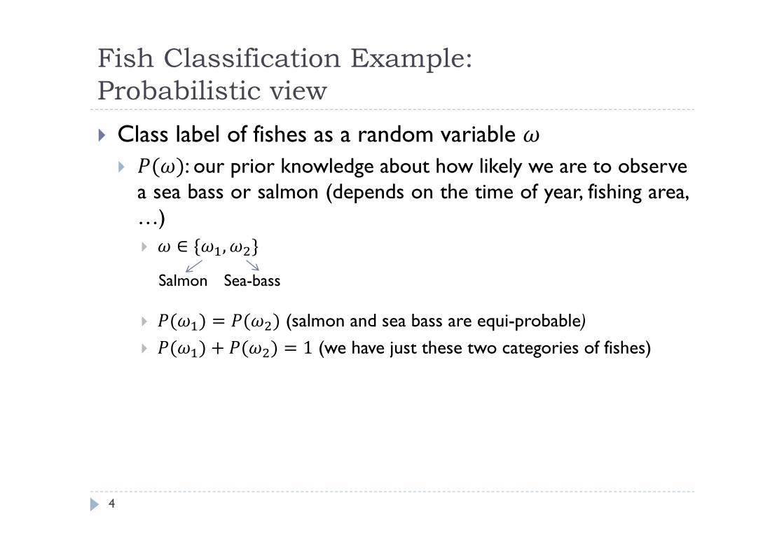
Fish Classification Example:Probabilistic view
4
Class label of fishes as a random variable ( ): our prior knowledge about how likely we are to observe
a sea bass or salmon (depends on the time of year, fishing area,…) ∈ { , } ( ) = ( ) (salmon and sea bass are equi-probable) ( ) + ( ) = 1 (we have just these two categories of fishes)
Salmon Sea-bass
Fish Classification Example:Probabilistic view (Cont’d)
5
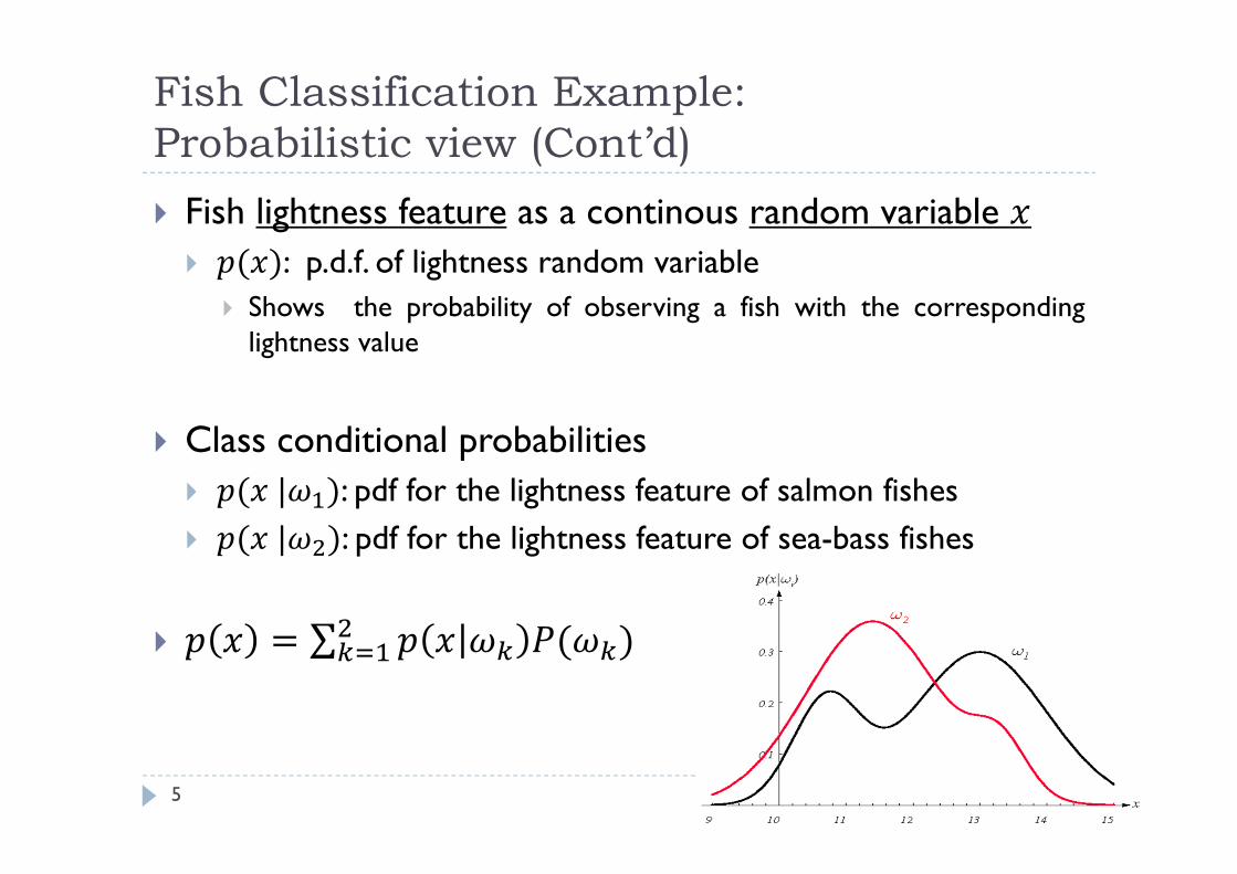
Fish lightness feature as a continous random variable ( ): p.d.f. of lightness random variable
Shows the probability of observing a fish with the correspondinglightness value
Class conditional probabilities ( | ): pdf for the lightness feature of salmon fishes ( | ): pdf for the lightness feature of sea-bass fishes
Fish Classification Example:Probabilistic view (Cont’d)
6
If we have a set of training examples we can estimate theclass conditional probabilities and also the priorprobabilities.
Now, suppose that we know these probabilities
Fish Classification Example:Bayes formula
7
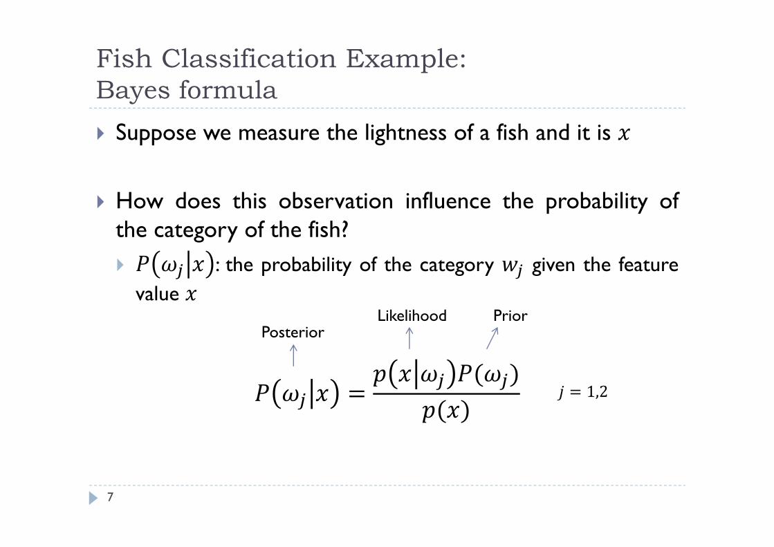
Suppose we measure the lightness of a fish and it is
How does this observation influence the probability ofthe category of the fish? : the probability of the category given the feature
valueLikelihood Prior
Posterior
= 1,2
Fish Classification Example:Bayesian Decision Rule
8
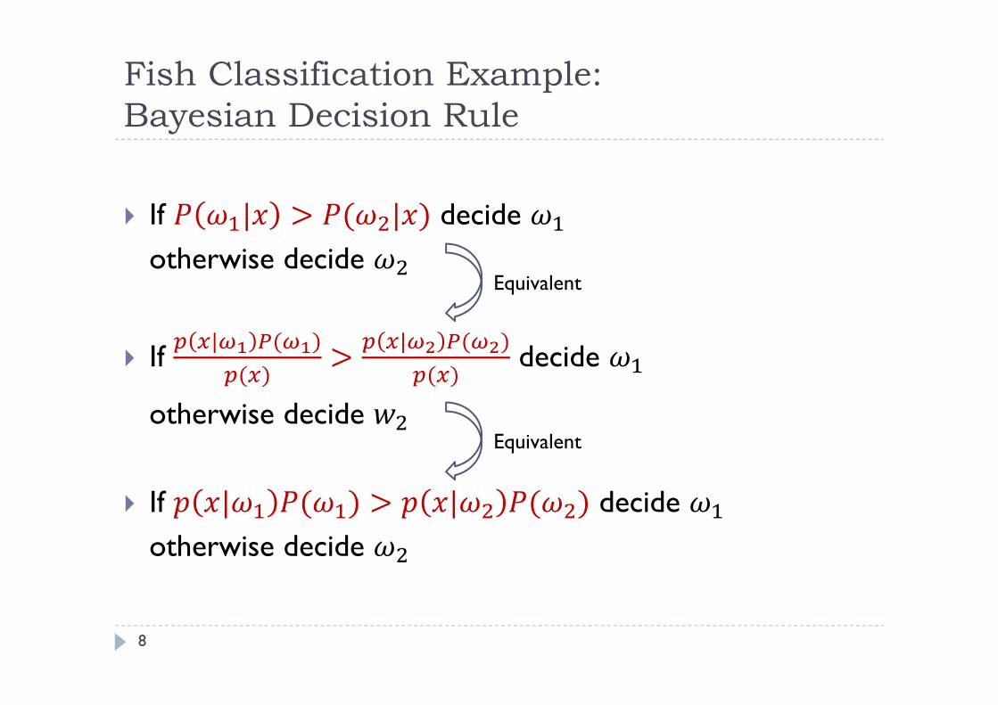
If decide otherwise decide
If | ( )( ) | ( )( ) decide
otherwise decide
If decide otherwise decide
Equivalent
Equivalent
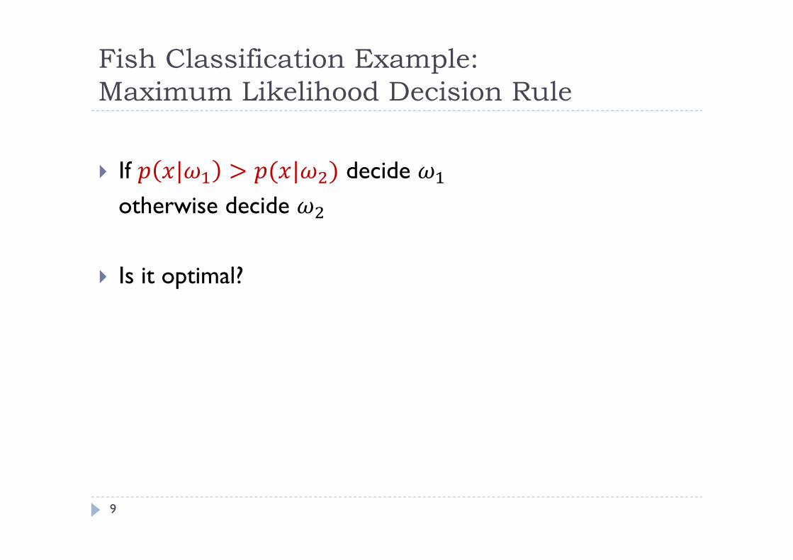
Fish Classification Example:Maximum Likelihood Decision Rule
9
If decide otherwise decide
Is it optimal?
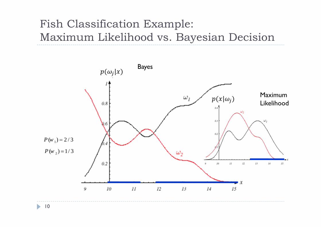
Fish Classification Example:Maximum Likelihood vs. Bayesian Decision
10
1( ) 2 / 3P w
2( ) 1/ 3P w
( | )( | )
Maximum Likelihood
Bayes
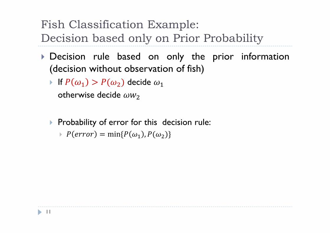
Fish Classification Example:Decision based only on Prior Probability
11
Decision rule based on only the prior information(decision without observation of fish) If > ( ) decide otherwise decide
Probability of error for this decision rule: = min { , ( )}
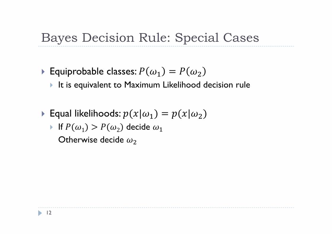
Bayes Decision Rule: Special Cases
12
Equiprobable classes: It is equivalent to Maximum Likelihood decision rule
Equal likelihoods: If ( 1) > ( 2) decide Otherwise decide
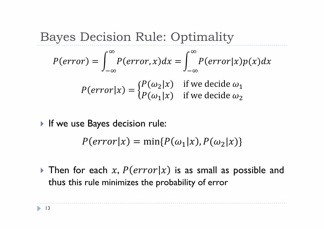
Bayes Decision Rule: Optimality
13
= , = | ( )= ( | ) if we decide ( | ) if we decide
If we use Bayes decision rule:
Then for each , is as small as possible andthus this rule minimizes the probability of error
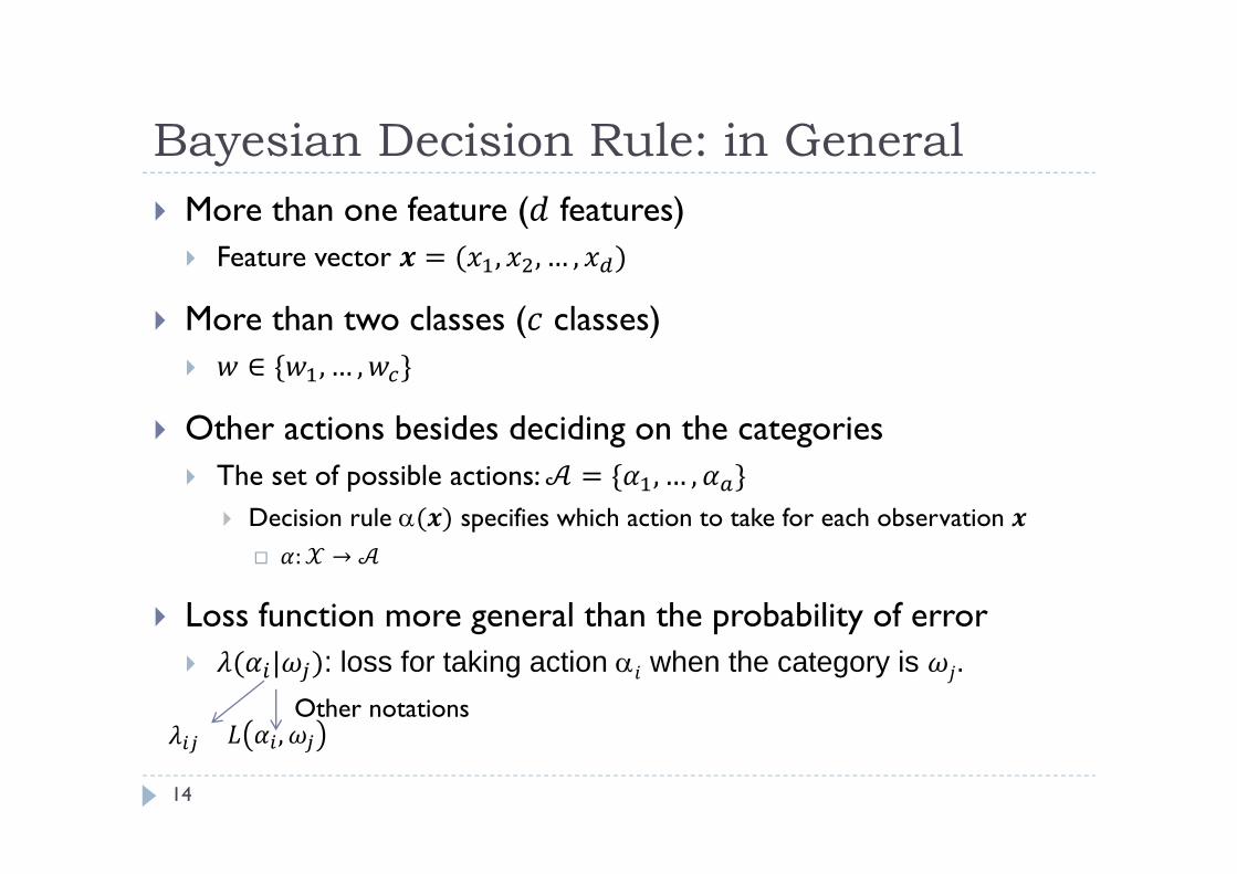
Bayesian Decision Rule: in General
14
More than one feature ( features) Feature vector = ( , , … , )
More than two classes ( classes) ∈ { , … , }
Other actions besides deciding on the categories The set of possible actions: = { , … , }
Decision rule ( ) specifies which action to take for each observation : →
Loss function more general than the probability of error ( | ): loss for taking action when the category is ., Other notations
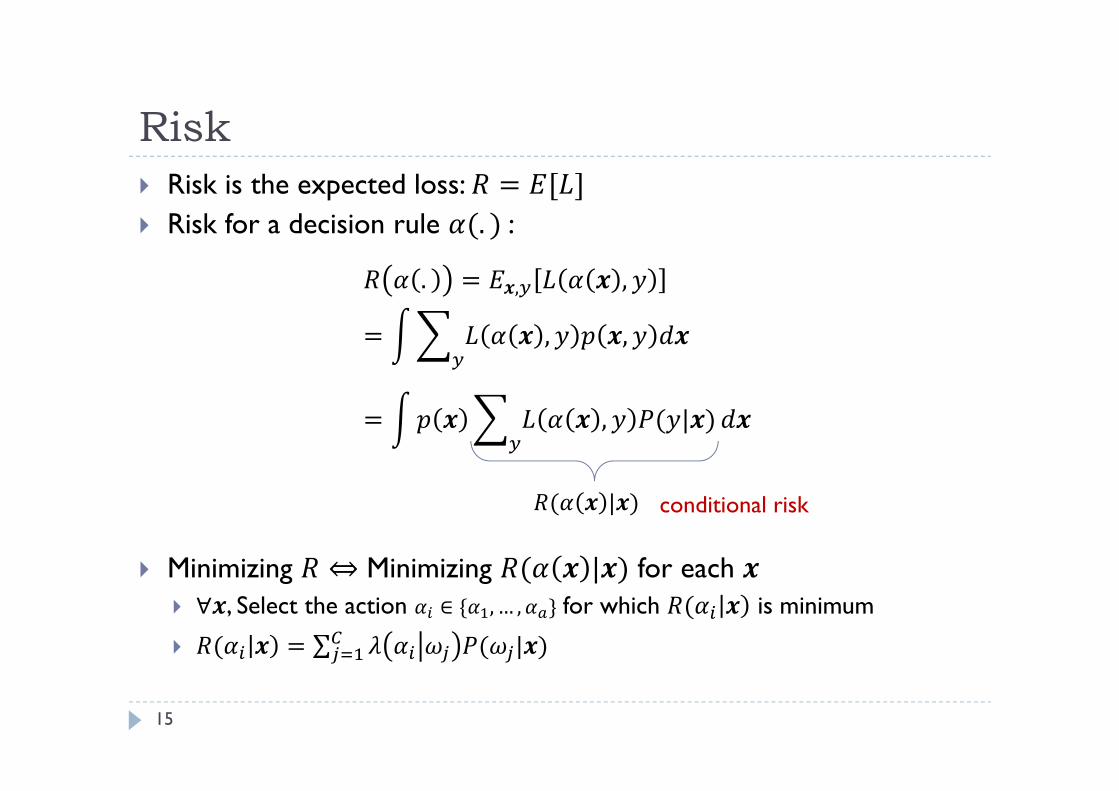
Risk
15
Risk is the expected loss: = [ ] Risk for a decision rule (. ) :
Minimizing ⇔ Minimizing ( | ) for each ∀ , Select the action ∈ { , … , } for which ( is minimum
( = ∑ ( | )( | )
. = , ,= , ,= , ( | )
conditional risk
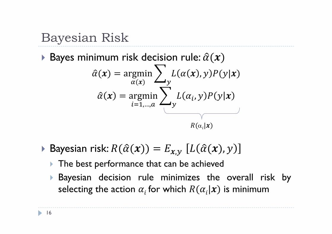
Bayesian Risk
16
Bayes minimum risk decision rule:( ) = argmin( ) , ( | )= argmin,…, , Bayesian risk: , The best performance that can be achieved Bayesian decision rule minimizes the overall risk by
selecting the action for which ( | ) is minimum
( | )
Conditional Risk: Two Category Example
17
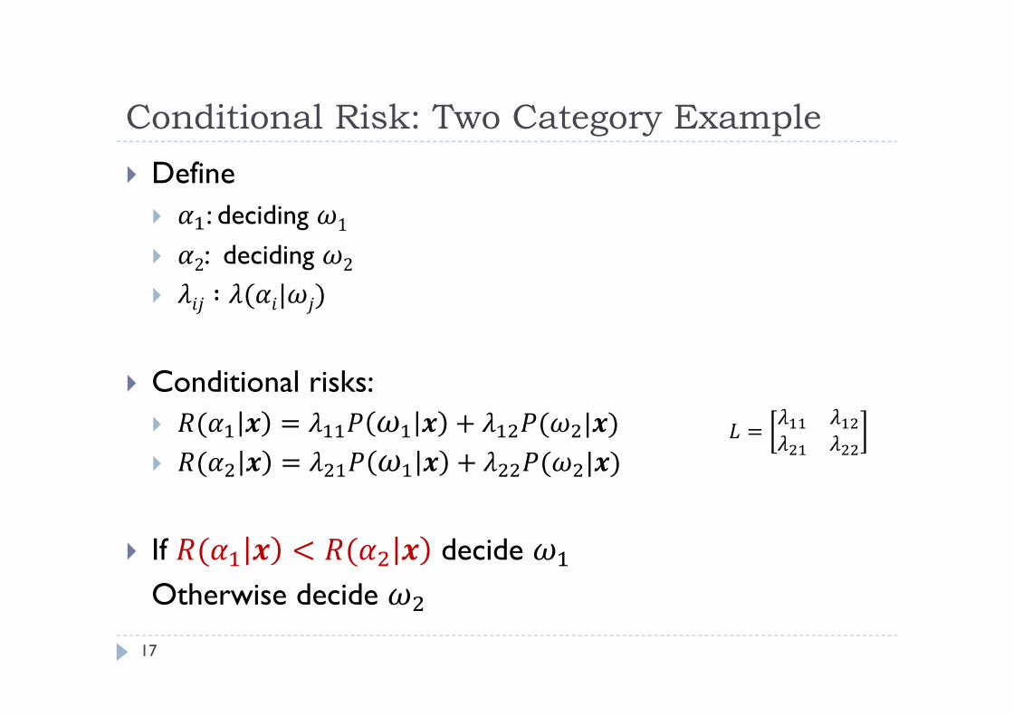
Define : deciding 1 2: deciding 2 ∶ ( | )
Conditional risks: ( = + ( | ) ( = + ( | )
If decide Otherwise decide
=
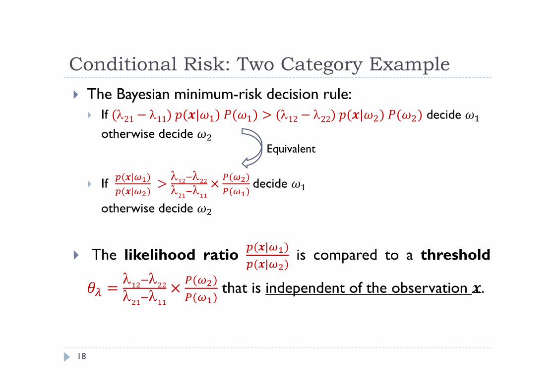
Conditional Risk: Two Category Example The Bayesian minimum-risk decision rule:
If (21 − 11) ( | ) ( ) > (12 − 22) ( | ) ( ) decide otherwise decide
If ( | )( | ) > × ( )( ) decide
otherwise decide
The likelihood ratio ( | )( | ) is compared to a threshold= × ( )( ) that is independent of the observation .
18
Equivalent
Example
19
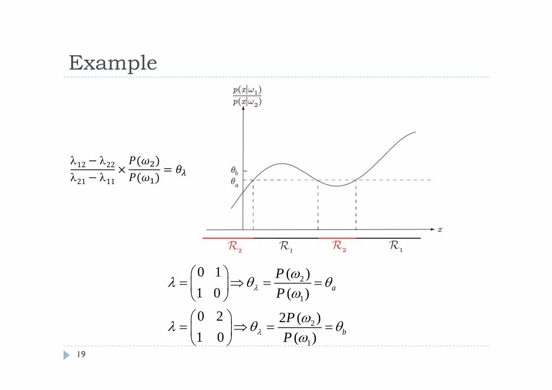
12 − 2221 − 11 × ( )( ) =
2
1
2
1
0 1 ( )1 0 ( )
0 2 2 ( )1 0 ( )
a
b
PP
PP
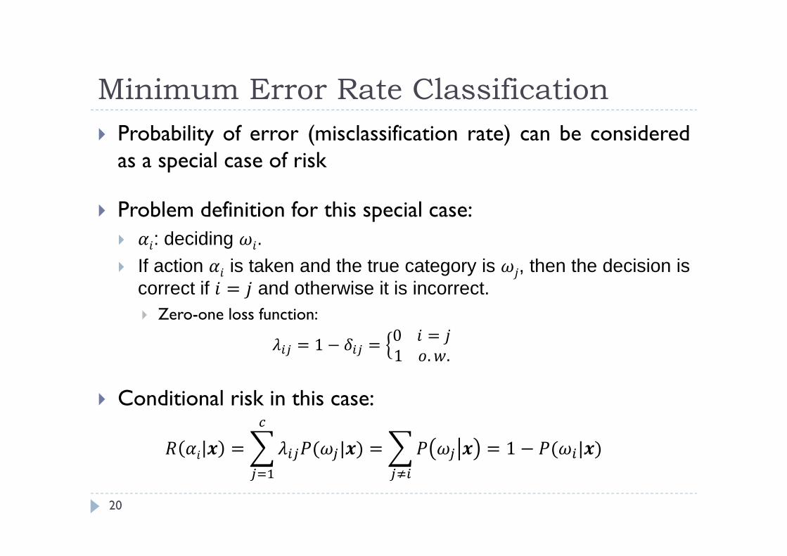
Minimum Error Rate Classification Probability of error (misclassification rate) can be considered
as a special case of risk
Problem definition for this special case: : deciding . If action is taken and the true category is , then the decision is
correct if = and otherwise it is incorrect. Zero-one loss function:= 1 − = 0 = 1 . .
Conditional risk in this case:= ( | ) = = 1 − ( | )20
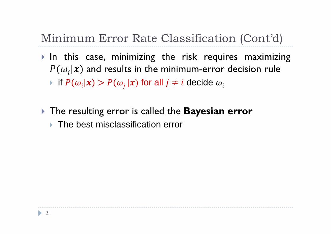
Minimum Error Rate Classification (Cont’d) In this case, minimizing the risk requires maximizing
and results in the minimum-error decision rule if ( | ) > ( | ) for all ≠ decide
The resulting error is called the Bayesian error The best misclassification error
21
Minimum Error Rate Classification (Cont’d)
22
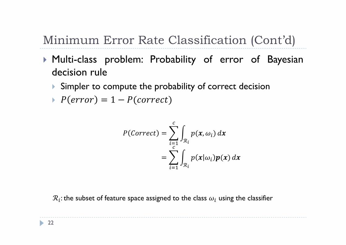
Multi-class problem: Probability of error of Bayesiandecision rule Simpler to compute the probability of correct decision = 1 − ( )
ℛ : the subset of feature space assigned to the class using the classifier
= ( , )ℛ = ( )ℛ
Probabilistic Discriminant Functions
23
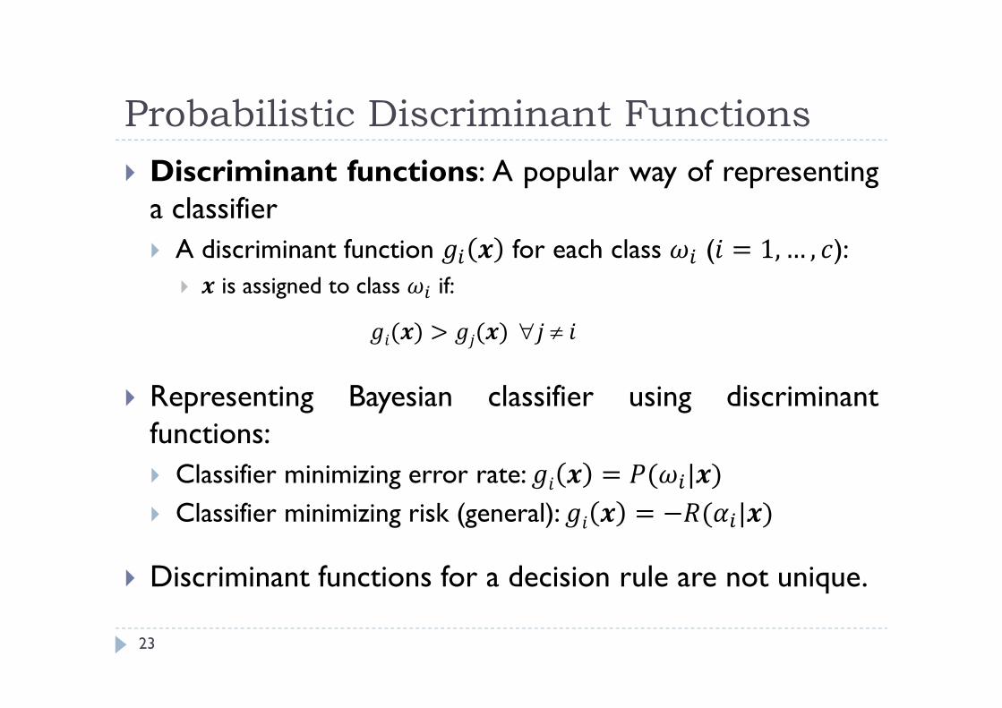
Discriminant functions: A popular way of representinga classifier A discriminant function for each class ( = 1, … , ):
is assigned to class if:( ) > ( ) Representing Bayesian classifier using discriminant
functions: Classifier minimizing error rate: = ( | ) Classifier minimizing risk (general): = − ( | )
Discriminant functions for a decision rule are not unique.

Discriminant Functions & Decision Surfaces
24
Using discriminant function, we can easily divide the featurespace into regions (each of them corresponds to a class) ℛ : Region of the -th class:∀ , ( ) > ( ) ⇒ ∈ ℛ
Decision surfaces (boundaries) can also be found usingdiscriminant functions Boundary of the ℛ and ℛ : ∀ , = ( )
Discriminant Functions: Gaussian Density
25
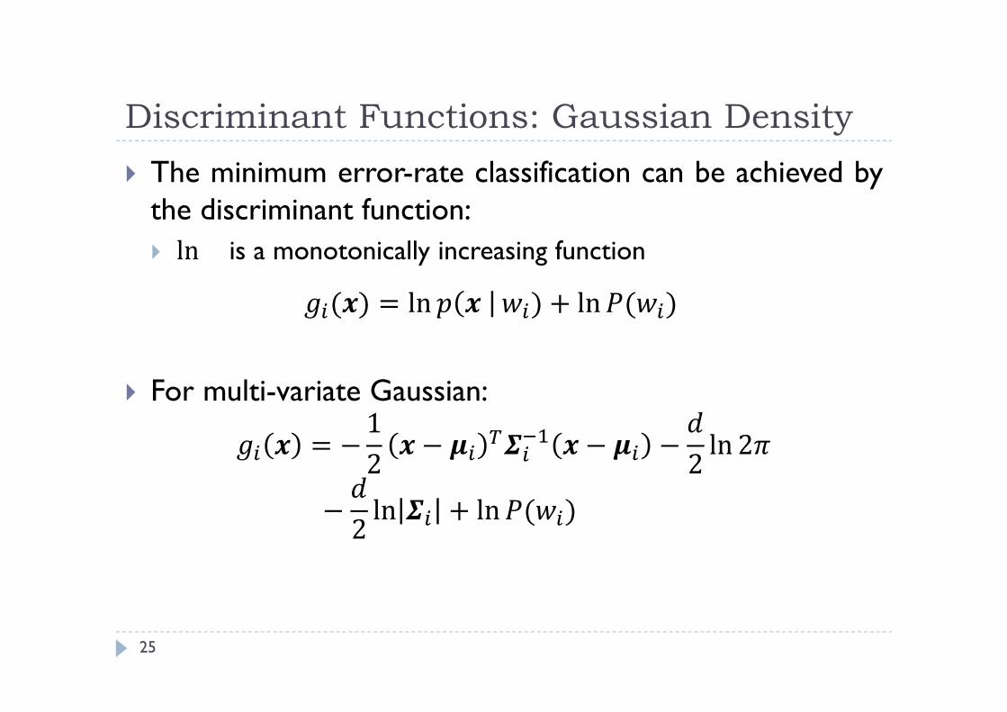
The minimum error-rate classification can be achieved bythe discriminant function: ln is a monotonically increasing function( ) = ln ) + ln ( )
For multi-variate Gaussian:= − 12 − − − 2 ln 2− 2 ln + ln ( )
Discriminant Functions: Gaussian densityCase I:
26
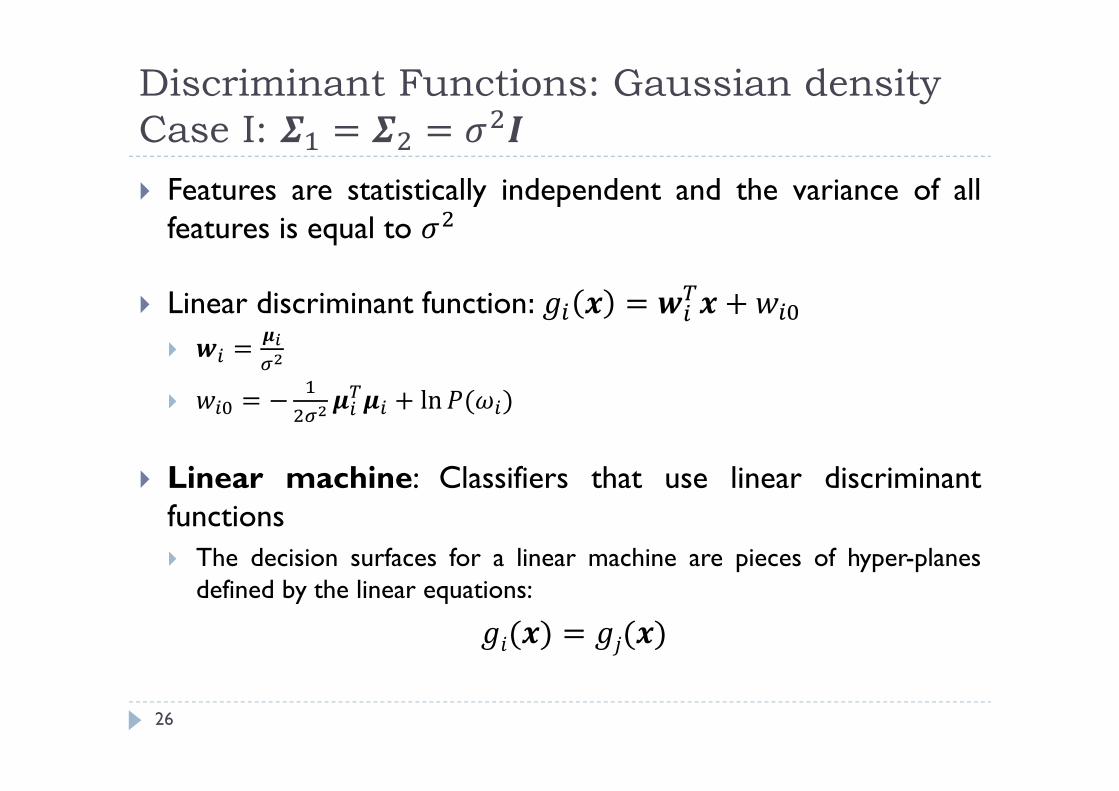
Features are statistically independent and the variance of allfeatures is equal to
Linear discriminant function: = + = = − + ln ( )
Linear machine: Classifiers that use linear discriminantfunctions The decision surfaces for a linear machine are pieces of hyper-planes
defined by the linear equations:( ) = ( )
Discriminant Functions: Gaussian DensityCase I:
27
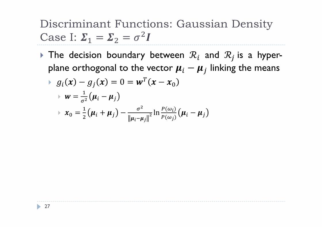
The decision boundary between and is a hyper-plane orthogonal to the vector linking the means − = 0 = −
= − = + − ln ( )( ) −

Discriminant Functions: Gaussian DensityCase I:
28
Discriminant Functions: Gaussian DensityCase I:
29
Discriminant Functions: Gaussian DensityCase I:
30
Special case 1 : Bayesian classifier is the minimum-distance classifier
if ∗ = argmin,.., − assign to ∗
Discriminant Functions: Gaussian DensityCase II:
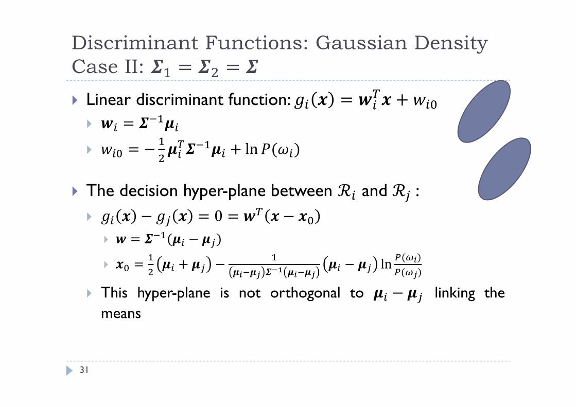
31
Linear discriminant function: = = − + ln ( )
The decision hyper-plane between and : − = 0 = −
= ( − ) = + − − ln ( )( )
This hyper-plane is not orthogonal to − linking themeans
Discriminant Functions: Gaussian DensityCase II:
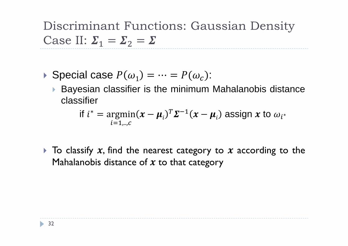
32
Special case 1 : Bayesian classifier is the minimum Mahalanobis distance
classifierif ∗ = argmin,.., − − assign to ∗
To classify , find the nearest category to according to theMahalanobis distance of to that category
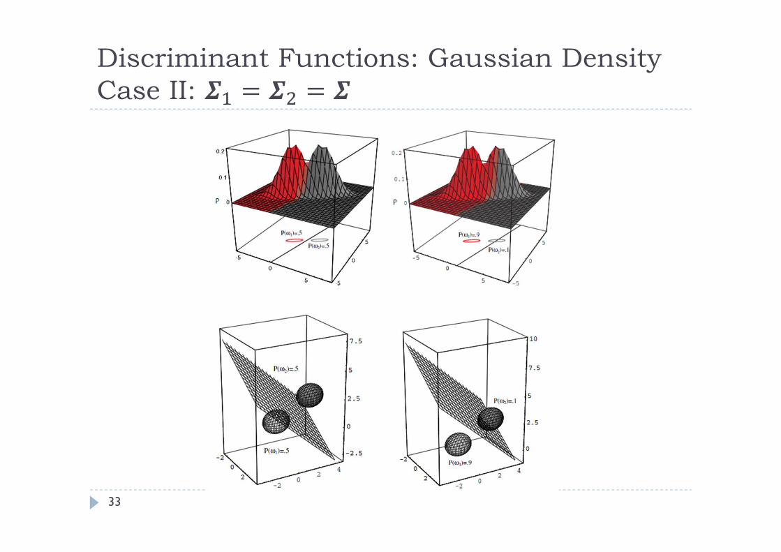
Discriminant Functions: Gaussian DensityCase II:
33
Discriminant Functions: Gaussian DensityCase III: arbitrary
34
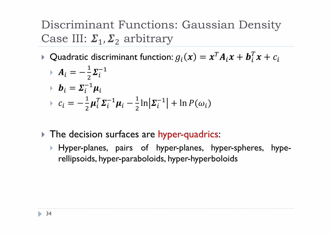
Quadratic discriminant function: = + + = − = = − − ln + ln ( )
The decision surfaces are hyper-quadrics: Hyper-planes, pairs of hyper-planes, hyper-spheres, hype-
rellipsoids, hyper-paraboloids, hyper-hyperboloids
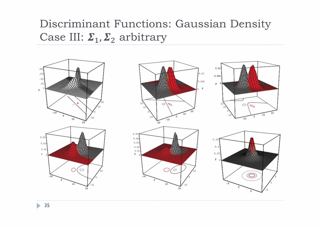
Discriminant Functions: Gaussian DensityCase III: arbitrary
35
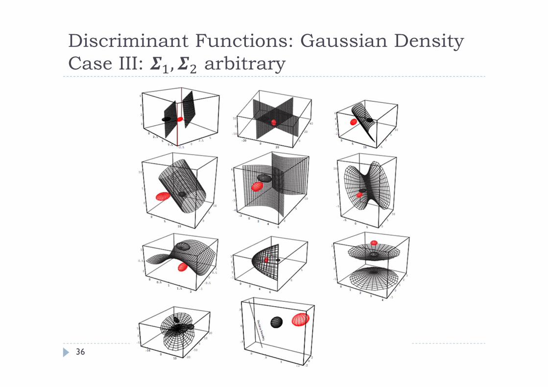
Discriminant Functions: Gaussian DensityCase III: arbitrary
36

Discriminant Functions: Gaussian DensityMulti Category
37
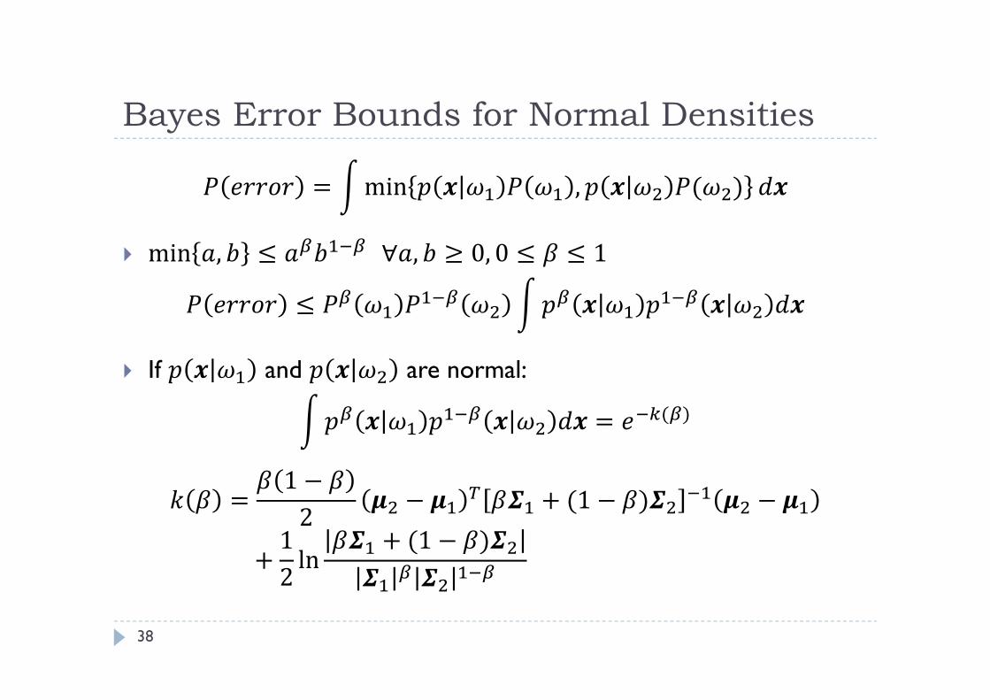
Bayes Error Bounds for Normal Densities
38
= min , ( ) min , ≤ ∀ , ≥ 0, 0 ≤ ≤ 1≤ If and are normal: = ( )
= 1 −2 − + (1 − ) −+ 12 ln + (1 − )
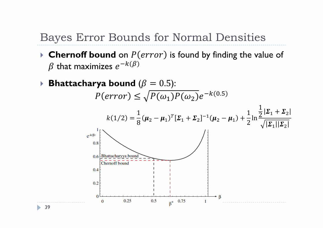
Bayes Error Bounds for Normal Densities
39
Chernoff bound on is found by finding the value ofthat maximizes ( )
Bhattacharya bound ( = 0.5):≤ ( ) ( ) ( . )1 2⁄ = 18 − + − + 12 ln 12 +

Minimax Criterion Design a classifier with a good performance on a range of prior
probabilities (Prior probabilities may vary widely and in an unpredictable way)
Set = 1 −= ℛ + ℛ
+ × ℛ + ℛ − ℛ − ℛ40
= + ( | )ℛ ++ ( | )ℛ
For a fix decision rule (i.e., fixed regions), risk is linear w.r.t. ( )
Minimax Criterion
41
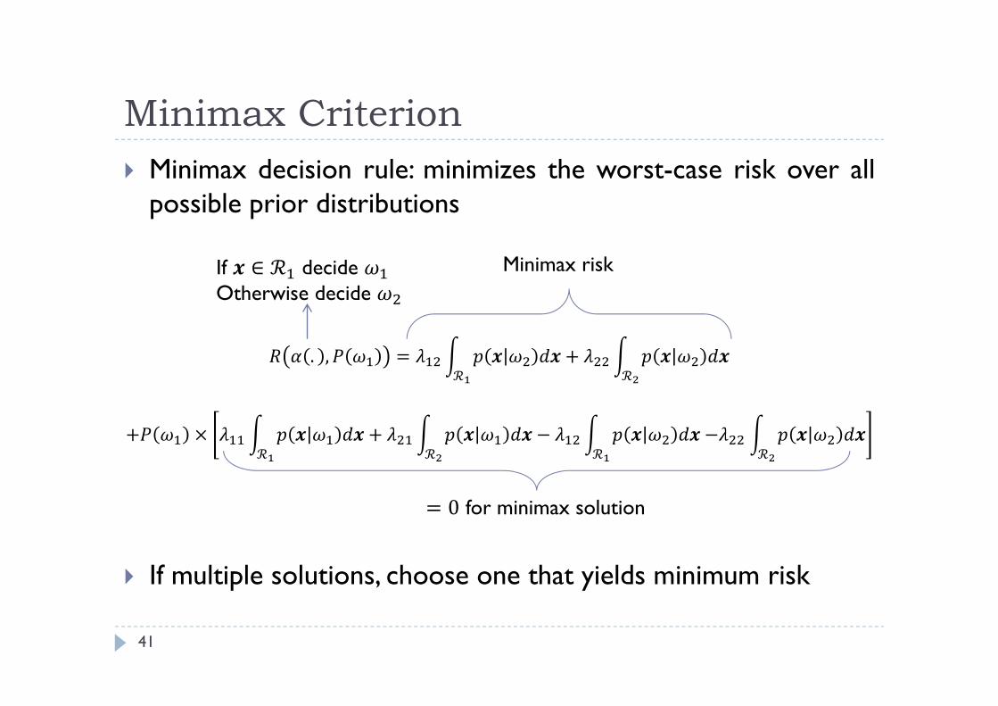
Minimax decision rule: minimizes the worst-case risk over allpossible prior distributions
. , = ℛ + ℛ+ × ℛ + ℛ − ℛ − ℛ
If multiple solutions, choose one that yields minimum risk
= 0 for minimax solution
Minimax riskIf ∈ ℛ decide Otherwise decide

Minimax Criterion
42
We are looking for the classifier which minimizes thismaximum risk: min( ) max ( (. , ( )), )
The line for each ( 1) is a tangent to ( . , ( 1) ).
( . , ( ) , ( ))( . , , 0 ≤ ( ) ≤ 1)
Risk for each ( ) when has also been found for the corresponding ( )
Risk for each ( ) when the decision rule is fixed for =
Neyman-Pearson Criterion Minimizing risk subject to a constraint
Example: maximizing the probability of detection, whileconstraining “probability of false-alarm ”. E.g. in a network intrusion detection system, we may need to
maximize the probability of detecting real attacks whileretaining the probability of false alarm below a threshold
N.-P. criterion is generally satisfied by adjusting boundariesnumerically However, for some distributions (e.g., Gaussian) analytical
solutions exist.
43
Definitions: TP, TN, FP, FN
44
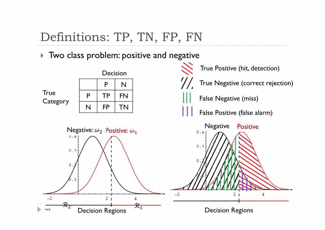
Decision
P N
P TP FN
N FP TN
Two class problem: positive and negative
True Category
PositiveNegative
Decision Regions
Positive: Negative:
Decision Regions
True Positive (hit, detection)
True Negative (correct rejection)
False Negative (miss)
False Positive (false alarm)
Positive
ℛℛ

Neyman-Pearson Criterion
45
The Neyman-Pearson criterion decision rule := argmin ( )subject to ( ) ≤ where ∈ [0, 1] is the “significance level” of the test
Assume that the probability of false alarm is a given , theNeyman-Pearson classifier will minimize the probability of miss 1 − is called “the power of the test” for the given significance level

Neyman-Pearson Criterion
46
Probability of false alarm: ℛ Probability of false negative: ℛ Neyman-Pearson rule that minimizes for a given is a
likelihood ratio test with a threshold :
Critical region:
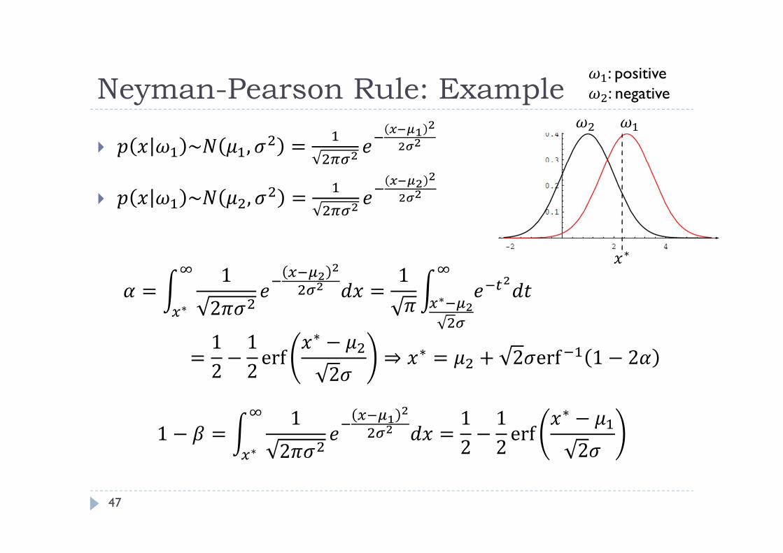
: positive: negative
Neyman-Pearson Rule: Example
47
~ , = ~ , =
= 12∗ = 1 ∗= 12 − 12 erf ∗ −2 ⇒ ∗ = + 2 erf 1 − 2
1 − = 12∗ = 12 − 12 erf ∗ −2
∗
: positive: negative
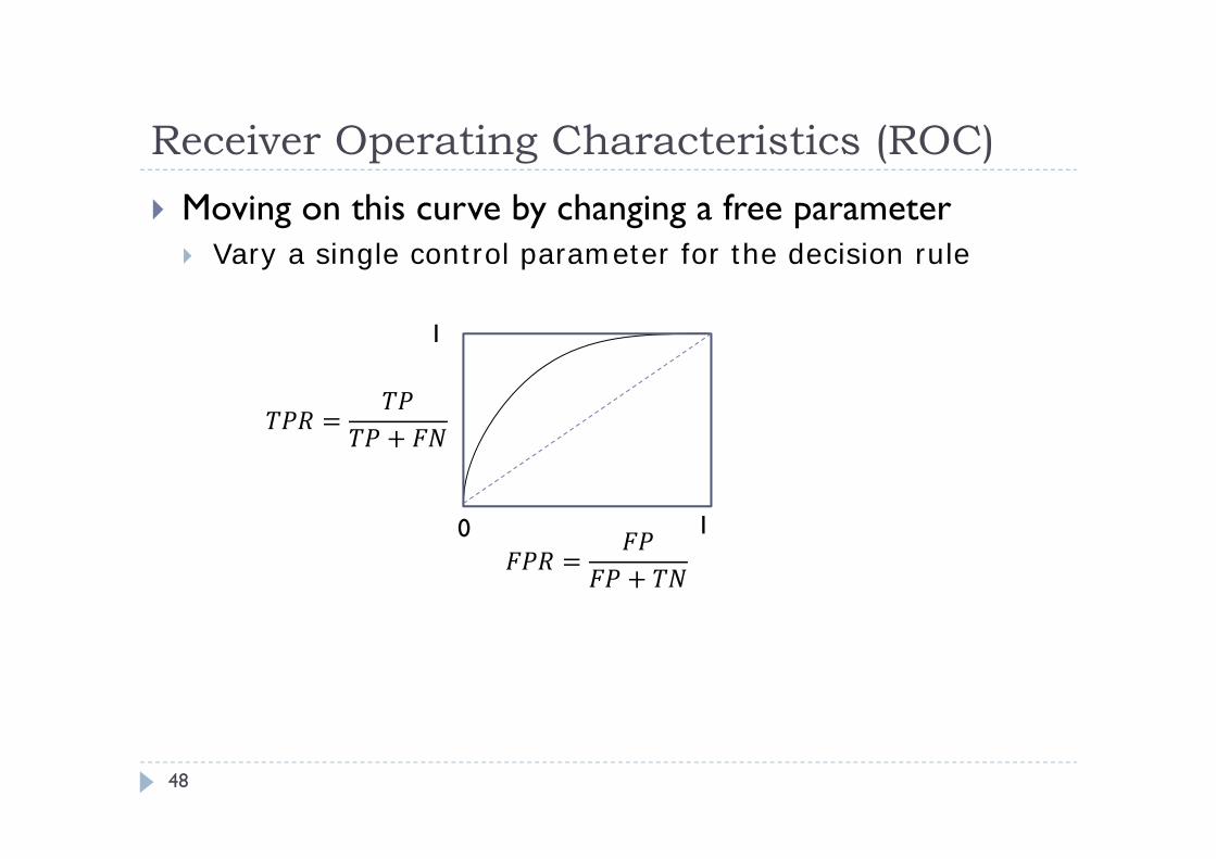
Receiver Operating Characteristics (ROC)
48
Moving on this curve by changing a free parameter Vary a single control parameter for the decision rule
= += +0 1
1