statistical evaluation of the response of intensity to large-scale forcing in the 2008 hwrf model...
TRANSCRIPT

Statistical Evaluation of the Response of Intensity to Large-Scale Forcing in the 2008 HWRF model
Mark DeMaria, NOAA/NESDIS/RAMMB Fort Collins, COBrian McNoldy, CSU, Fort Collins, CO
Presented at the HFIP Diagnostics Workshop
May 5, 2009

Outline
• Motivation
• HWRF Sample
• Evolution of large scale forcing in HWRF– Lower boundary– Vertical shear
• Evaluation of storm response to forcing – Fitting LGEM model to HWRF forecasts– Comparison with fitting LGEM to observations


Intensification Factors in SHIPS Model
1) Center over Land• Time since landfall, fraction of circulation over land
2) Center over Water
Normalized Regression Coefficients at 48 hr for 2009 SHIPS Model
-0.6
-0.4
-0.2
0
0.2
0.4
0.6
0.8
1
Ju
lian
Da
y
Pe
rsis
ten
ce
Vm
ax
*Pe
r
Zo
na
l mo
tio
n
Ste
eri
ng
La
ye
r
GO
ES
Co
ld C
lou
d
GO
ES
As
ym
.
SS
T P
ote
nti
al
SS
T P
ote
nti
al *
*2
Vm
ax
t=
0
Oc
ea
n H
ea
t C
on
ten
t
Sh
ea
r
Sh
ea
r*L
at
Sh
ea
r*V
ma
x
Sh
ea
r D
ire
cti
on
GF
S v
ort
ex
85
0 h
Pa
En
v V
ort
20
0 h
Pa
En
v D
iv
T 2
00
hP
a
T 2
50
hP
a
Ve
rt S
tab
ility
Mid
-le
ve
l RH
No
rma
lize
d R
eg
res
sio
n C
oe
ffic
ien
t

Preliminary Analysis of HWRF
• Consider 3 error sources– Accuracy of track forecasts
• Over land versus over water
– SST along forecast track• Related to MPI
– Shear along forecast track
• Compare track, SST and shear errors to HWRF intensity errors
• How to HWRF storms respond to SST and shear forcing compared to real storms?

Summary of HWRF Cases• Atlantic • East Pacific
Total - 576 HWRF runs during 2008 * - 7532 individual times to compare an HWRF analysis or forecast to Best Track data *
* HWRF runs only counted for named storms in Best Track database
0
10
20
30
40
50
60
70
Arthur
Bertha
Cristo
bal
Dolly
Edouard
Fay
Gustav
HannaIk
e
Jose
phine
Kyle
Laura
Mar
coNana
Omar
Palom
a
No
. Cas
es
0
10
20
30
40
50
60
70
Alma
Boris
Christin
a
Douglas
Elida
Faust
o
Genevie
ve
Hernan
Isel
leJu
lio
Karina
Lowell
Mar
ie
Norbert
OdilePolo
No
. Cas
es
N=331 N=245

Initial Positions of 2008 HWRF Cases

Simple “SHIPS-type”text output files created from HWRF grid files for preliminary analysis

Error Methods
BIAS MEAN ABSOLUTE ERROR
LATITUDE: increasing toward north LONGITUDE: increasing toward east CENTER LOCATION: positioned at lowest SLP in HWRF nested grid DISTANCE TO LAND: positive over ocean, negative over land, HWRF and BTRK use identical land masks SST: five closest gridpoints under storm center in HWRF VERT SHEAR: 850-200hPa winds averaged from 300-350km around storm center in HWRF nested grid (200-800km in BTRK) MAX WIND: strongest 10m wind in HWRF nested grid
Ground truth for lat, lon, max wind from NHC best track Ground “truth” for SST and Shear from SHIPS developmental dataset
i
Ni
ii BTRKHWRF
N
1
1
Ni
iii BTRKHWRF
N 1
1

Storm Errors : Maximum Wind
BIAS MEAN ABSOLUTE ERROR

Lat/Lon Track Biases
Latitude Bias Longitude Bias

Track Errors : Center Location
Mean Absolute Errors

Track Errors : 30hr,60hr Truth Table

Track Errors : 90hr,120hr Truth Table

Track Errors : Correct Surface Type

Storm Errors : Sea Surface Temp
BIAS MEAN ABSOLUTE ERROR

Storm Errors : Vertical Shear
BIAS MEAN ABSOLUTE ERROR
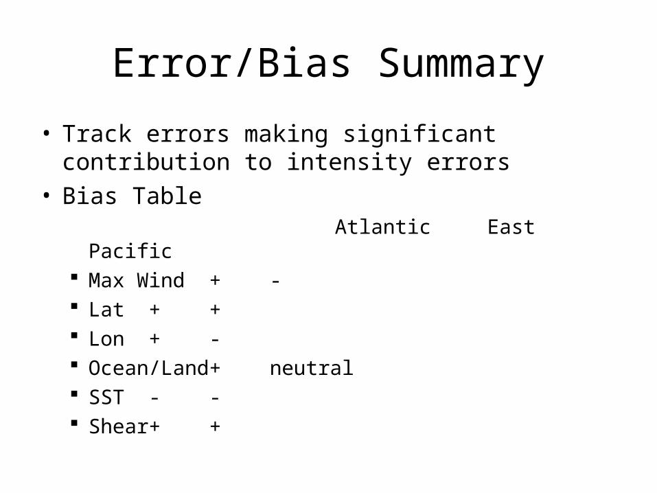
Error/Bias Summary
• Track errors making significant contribution to intensity errors
• Bias Table Atlantic East Pacific Max Wind + - Lat + + Lon + - Ocean/Land + neutral SST - - Shear + +

Evaluation of Storm Response to Forcing
• Use simplified version of LGEM model– Includes only MPI and vertical shear terms
• Use LGEM adjoint to find optimal coefficients for MPI and shear terms
• Fit to HWRF forecasts and to observations
• Compare fitted coefficients
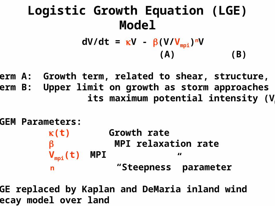
Logistic Growth Equation (LGE) Model
dV/dt = V - (V/Vmpi)nV (A) (B)
Term A: Growth term, related to shear, structure, etc Term B: Upper limit on growth as storm approaches its maximum potential intensity (Vmpi)
LGEM Parameters: (t) Growth rate MPI relaxation rate Vmpi(t) MPI n “Steepness” parameter
LGE replaced by Kaplan and DeMaria inland wind decay model over land

Analytic LGE Solutions for Constant , , n, Vmpi
Vs = Steady State V = Vmpi(/)1/n Let U = V/Vs and T = tdU/dT = U(1-Un) U(t) = Uo{enT/[1 + (enT-1)(Uo)n]}1/n
0
0.2
0.4
0.6
0.8
1
1.2
1.4
1.6
1.8
0 0.5 1 1.5 2 2.5 3 3.5 4
T
U
Vo/Vs=1.6Vo/Vs=1.3Vo/Vs=1.0Vo/Vs=0.7Vo/Vs=0.4Vo/Vs=0.1
0
0.2
0.4
0.6
0.8
1
1.2
1.4
1.6
1.8
0 0.5 1 1.5 2 2.5 3 3.5 4
t/k
V/V
s
Vo/Vs=1.6Vo/Vs=1.3Vo/Vs=1.0Vo/Vs=0.7Vo/Vs=0.4Vo/Vs=0.1
0 0
U
T
U
n=3 n=3
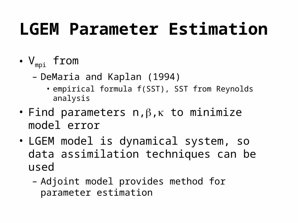
LGEM Parameter Estimation
• Vmpi from – DeMaria and Kaplan (1994)
• empirical formula f(SST), SST from Reynolds analysis
• Find parameters n,, to minimize model error• LGEM model is dynamical system, so data
assimilation techniques can be used– Adjoint model provides method for parameter
estimation

Application of Adjoint LGE Model• Discretized forward model: V0 = Vobs(t=0)
V+1 = V + [V -(V /Vmpi )nV ]t, =1,2,…T• Error Function: E = ½ (V -Vobs )2
• Add forward model equations as constraints: J = E + {V+1 - V - [V -(V /Vmpi )nV ]t}• Set dJ/dV = to give adjoint model for
T = - (VT-VobsT), = +1{-(n+1)(V/Vmpi)n]t} - (V-Vobs), =T-1,T-2,…• Calculate gradient of J wrt to unknown parameters dJ/d = - t V-1
dJ/dn = t (V-1/Vmpi-1)nV-1
dJ/d = t (V-1/Vmpi-1)n ln(V-1/Vmpi -1)nV-1
• Use gradient descent algorithm to find optimal parameters
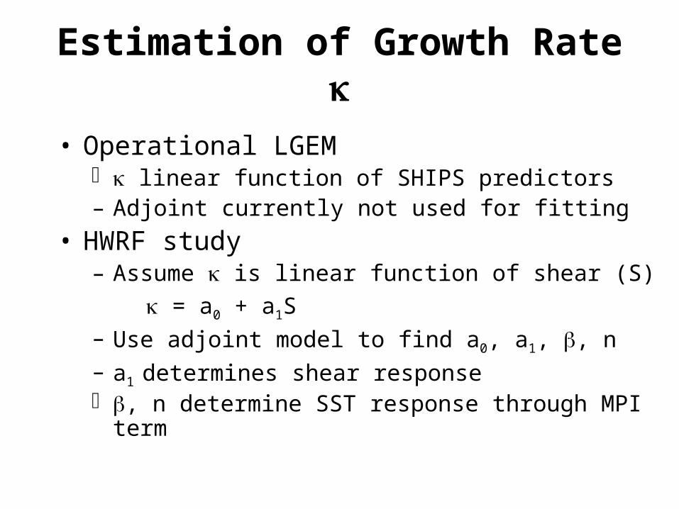
Estimation of Growth Rate
• Operational LGEM linear function of SHIPS predictors– Adjoint currently not used for fitting
• HWRF study– Assume is linear function of shear (S)
= a0 + a1S– Use adjoint model to find a0, a1, , n– a1 determines shear response , n determine SST response through MPI term

Example of LGEM Fitting
• Hurricane Omar (2008)• Find 4 constants to
minimize 5-day LGEM forecast
• Input:– Observed track, SST,
shear • Optimal parameters
= 0.034 n =2.61a1=-0.026 a0=0.017
-1 = 29 hr |a1-1|=36 hr

Optimal LGEM Forecast with Observational Input
0
20
40
60
80
100
120
140
160
0 12 24 36 48 60 72 84 96 108 120
Time (hr)
Ma
x W
ind
(k
t) o
r S
he
ar
(kt)
MPI
Best Track
LGEM
Shear
Mean Absolute Intensity Error = 6.3 kt
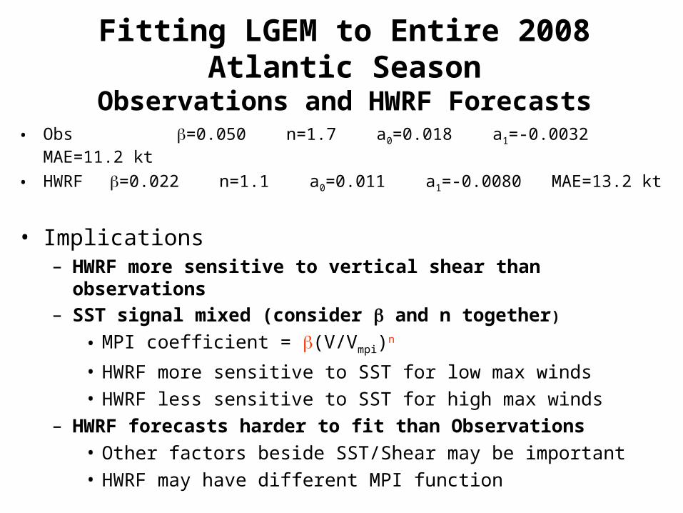
Fitting LGEM to Entire 2008 Atlantic SeasonObservations and HWRF Forecasts
• Obs =0.050 n=1.7 a0=0.018 a1=-0.0032 MAE=11.2 kt
• HWRF =0.022 n=1.1 a0=0.011 a1=-0.0080 MAE=13.2 kt
• Implications– HWRF more sensitive to vertical shear than observations– SST signal mixed (consider and n together)
• MPI coefficient = (V/Vmpi)n
• HWRF more sensitive to SST for low max winds• HWRF less sensitive to SST for high max winds
– HWRF forecasts harder to fit than Observations• Other factors beside SST/Shear may be important• HWRF may have different MPI function

Summary
• Preliminary diagnostic analysis of 2008 HWRF runs
• Track error may be significant contribution to Atlantic intensity error
• Biases differ between Atlantic and east Pacific– Track, SST, Shear biases help explain East Pacific
intensity bias, but not Atlantic
• Preliminary analysis using LGEM fit indicates response to SST and Shear in HWRF is different than observations
Future Plans• Continue current analysis on east Pacific cases• Investigate vertical instability impact on intensity
changes• Examine HWRF MPI relationships• Evaluation HWRF in “GOES IR space”
– Apply radiative transfer to HWRF output to create simualted imagery
– Need vertical profiles of T, RH and all condensate variables
• Develop applications of ensemble forecasts using NHC wind probability model framework

Example of Simulated ImageryHurricane Wilma 2005
GOES-East Channel 3 Channel 3 from RAMS Model Output

Back-Up Slides

Summary of Cases• Atlantic • East Pacific
Total
# OF RUNS # OF INDIV TIMESARTHUR 4 14BERTHA 62 1155
CRISTOBAL 14 119DOLLY 16 231
EDOUARD 8 44FAY 34 678
GUSTAV 29 554HANNA 38 603
IKE 50 840JOSEPHINE 15 120
KYLE 13 104LAURA 9 45MARCO 5 15NANA 5 20OMAR 15 120
PALOMA 14 105331 4767
# OF RUNS # OF INDIV TIMES4 18
27 3779 456 27
23 35522 29122 25224 2948 459 633 9
18 17122 25229 43113 1096 26
245 2765
- 576 HWRF runs during 2008 * - 7532 individual times to compare an HWRF analysis or forecast to Best Track data *
* HWRF runs only counted for named storms in Best Track database
ALMABORISCHRISTINA

Track Errors : Distance to Land
BIAS MEAN ABSOLUTE ERROR

Track Errors : 0hr Truth Table
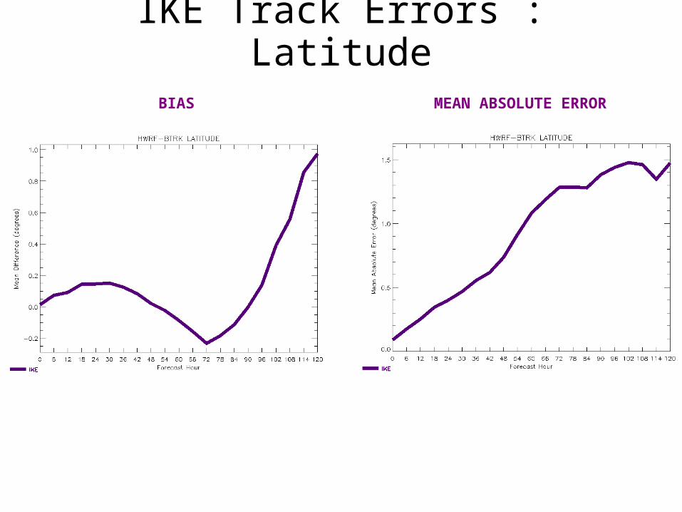
IKE Track Errors : Latitude
BIAS MEAN ABSOLUTE ERROR
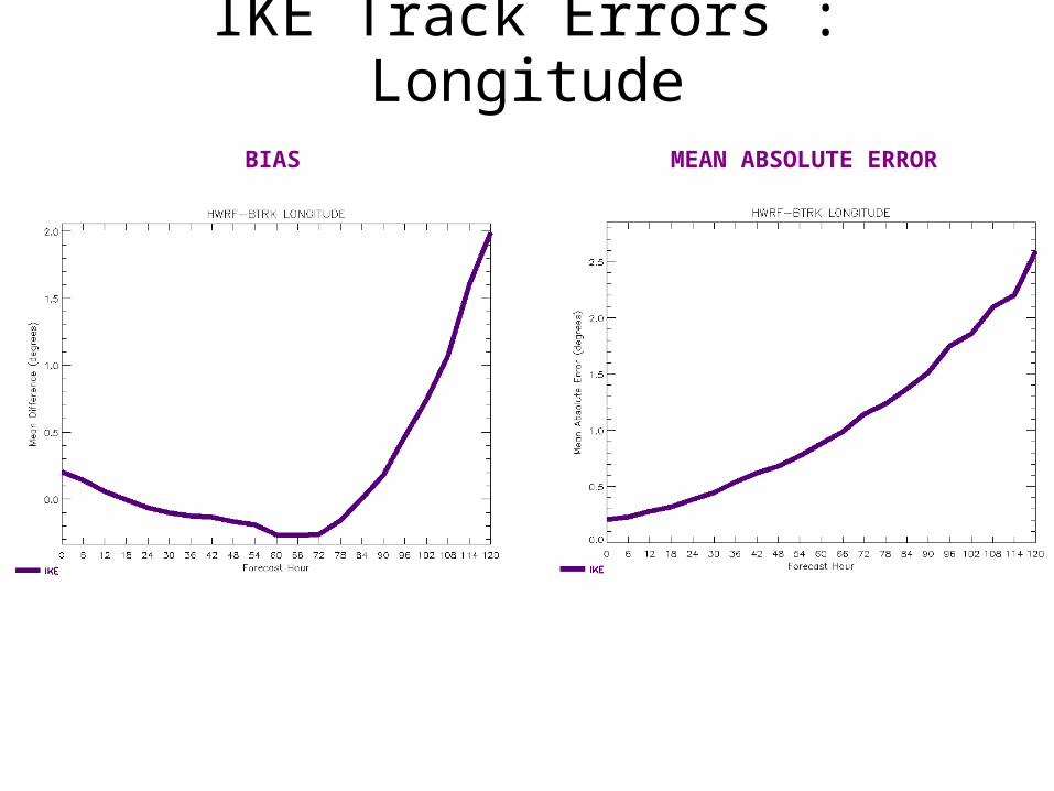
IKE Track Errors : Longitude
BIAS MEAN ABSOLUTE ERROR
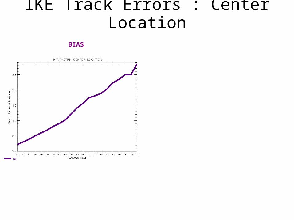
IKE Track Errors : Center Location
BIAS

IKE Track Errors : Distance to Land
BIAS MEAN ABSOLUTE ERROR

IKE Track Errors : 0hr Truth Table

IKE Track Errors : 30hr,60hr Truth Table

IKE Track Errors : 90hr,120hr Truth Table

IKE Track Errors : Correct Land Type

IKE Storm Errors : Sea Surface Temp
BIAS MEAN ABSOLUTE ERROR
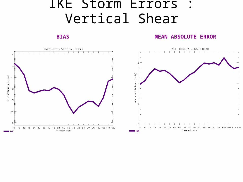
IKE Storm Errors : Vertical Shear
BIAS MEAN ABSOLUTE ERROR

IKE Storm Errors : Maximum Wind
BIAS MEAN ABSOLUTE ERROR