Statistical Learning Theory: A Tutorial

Sanjeev R. Kulkarni and Gilbert Harman∗

February 20, 2011

Abstract

In this article, we provide a tutorial overview of some aspects of statistical learningtheory, which also goes by other names such as statistical pattern recognition, nonparametricclassification and estimation, and supervised learning. We focus on the problem of two-classpattern classification for various reasons. This problem is rich enough to capture many ofthe interesting aspects that are present in the cases of more than two classes and in theproblem of estimation, and many of the results can be extended to these cases. Focusingon two-class pattern classification simplifies our discussion, and yet it is directly applicableto a wide range of practical settings.

We begin with a description of the two class pattern recognition problem. We thendiscuss various classical and state of the art approaches to this problem, with a focus onfundamental formulations, algorithms, and theoretical results. In particular, we describenearest neighbor methods, kernel methods, multilayer perceptrons, VC theory, support vec-tor machines, and boosting.

Index Terms: statistical learning, pattern recognition, classification, supervised learning,kernel methods, neural networks, VC dimension, support vector machines, boosting

1 Introduction

In this paper, we focus on the problem of two-class pattern classification — classifying an objectinto one of two categories based on several observations or measurements of the object. Morespecifically, we are interested in methods for learning rules of classification.

Consider the problem of learning to recognize handwritten characters or faces or otherobjects from visual data. Or, think about the problem of recognizing spoken words. While

∗Sanjeev R. Kulkarni is with the Department of Electrical Engineering, Princeton University, Princeton, NJ08544. His email address is kulkarni@princeton.edu. Gilbert Harman is with the Department of Philosophy,Princeton University, Princeton, NJ 08544. His email address is harman@princeton.edu.

1

humans are extremely good at these types of classification problems in many natural settings,it is quite difficult to design automated algorithms for these tasks with anywhere near the per-formance and robustness of humans. Even after more than a half century of effort in fields suchas electrical engineering, mathematics, computer science, statistics, philosophy, and cognitivescience, humans can still far outperform the best pattern classification algorithms that havebeen developed. That said, enormous progress has been made in learning theory, algorithms,and applications. Results in this area are deep and practical and are relevant to a range ofdisciplines.

Our aim in this paper is to provide an accessible introduction to this field, either as afirst step for those wishing to pursue the subject in more depth, or for those desiring a broadunderstanding of the basic ideas. Our treatment is essentially a condensed version of the book[9], which also provides an elementary introduction to the topics discussed here, but in moredetail. Although many important aspects of learning are not covered by the model we focus onhere, we hope this paper provides a valuable entry point to this area. For further reading, weinclude a number of references at the end of this paper. The references included are all textbooksor introductory, tutorial, or survey articles. These references cover the topics discussed here aswell as many other topics in varying levels of detail and depth. Since this paper is intended asa brief, introductory tutorial, and because all the material presented here is very standard, werefrain from citing original sources, and instead refer the reader to the references provided atthe end of this paper and the additional pointers contained therein.

2 The Pattern Recognition Problem

In the pattern classification problem, we observe an object and wish to classify it into one of twoclasses, which we might call 0 and 1 (or −1 and 1). In order to decide either 0 or 1, we assumewe have access to measurements of various properties of the object. These measurements maycome from sensors that capture some physical variables of interest, or features, of the object.

For simplicity, we represent each measured feature by a single real number. Although insome applications certain features may not be very naturally represented by a number, thisassumption allows discussion of the most common learning techniques that are useful in manyapplications. The set of features can be put together to form a feature vector. Suppose thereare d features with the value of the features given by x1, x2, . . . , xd. The feature vector isx = (x1, x2, . . . , xd), which can be thought of as a point or a vector in d-dimensional space Rd,which we call feature space.

One concrete application is image classification. The features in this case might be theintensities of pixels in the image. For an N ×N gray scale image the total number of featureswould be d = N2. In the case of a color image, each pixel can be considered as providing 3measurements, corresponding to the intensities of each of three color components. In this case,

2

there are d = 3N2 features. For even a modest size image, the dimension of the feature spacecan be quite large.

In most applications, the class to which an object belongs is not uniquely and definitivelydetermined by its feature vector. There are some fundamental reasons for this. First, althoughit would be nice if the measured features capture all the properties of the object important forclassification, this usually is not the case. Second, depending on the application and the specificmeasurements, the feature values may be noisy. For these reasons, a statistical formulation forthe pattern recognition problem is very useful.

We assume that there are prior probabilities P (0) and P (1) of observing an object fromeach of the two classes. The feature vector of the object is related to the class to which theobject belongs. This is described through conditional probability densities p(x|0) and p(x|1).Equivalently, let y ∈ 0, 1 be the label associated with x (i.e., the actual class to which theobject belongs). Then, we can think of the pair (x, y) as being drawn from a joint distributionP (x, y).

When we observe a feature vector x, our problem is to decide either 0 or 1. So, a decisionrule (or classification rule) can be thought of as a mapping c : Rd → 0, 1, where c(x) indicatesthe decision when feature vector x is observed. Equivalently, we can think of a decision ruleas a partition of Rd into two sets Ω0 and Ω1 that correspond to those feature vectors thatget classified as 0 and 1, respectively. For technical/mathematical reasons we do not considerthe set of all possible subsets of Rd as potential decision rules, but rather restrict attention todecision rules that are measurable.

Out of the enormous collection of all possible decision rules, we would like to select one thatperforms well. We make a correct decision if our decision c(x) is equal to the label y. A naturalsuccess criterion is the probability that we make a correct decision. We would like a decisionrule that maximizes this probability, or equivalently, that minimizes the probability of error.For a decision rule c, the probability of error of c, denoted R(c), is given by

R(c) = E[(c(x)− y)2] = P (0)P (Ω1|0) + P (1)P (Ω0|1).

In the ideal (and unusual) case, where the underlying probabilistic structure is known, thesolution to the classification problem is well known and is a basic result from statistics. Onthe assumption that the underlying probabilities P (0), P (1) and p(x|0), p(x|1) are all known,we can compute the so-called posterior probabilities P (0|x) and P (1|x) using Bayes theorem.Specifically, the unconditional distribution P (x) is given by

P (x) = P (0)P (x|0) + P (1)P (x|1) (1)

and probabilities P (0|x) and P (1|x) are then given by

P (0|x) =P (0)P (x|0)

P (x)(2)

3

P (1|x) =P (1)P (x|1)

P (x)(3)

Once we have the posterior probabilities, the best decision is simply to choose the classwith larger conditional probability – namely, decide 0 if P (0|x) > P (1|x) and decide 1 ifP (1|x) > P (0|x). If P (0|x) = P (1|x), then it doesn’t matter what we decide. This classificationrule is called Bayes decision rule, or sometimes simply Bayes rule.

Bayes decision rule is optimal in the sense that no other decision rule has a smaller proba-bility of error. The error rate of Bayes decision rule, denoted by R∗, is given by

R∗ =∫Rd

minP (0|x), P (1|x)p(x) dx (4)

Clearly, 0 ≤ R∗ ≤ 1/2 but we can’t say more without additional assumptions.

Finding Bayes decision rule requires knowledge of the underlying distributions, but typicallyin applications these distributions are not known. In fact, in many applications, even the formof or approximations to the distributions are unknown. In this case, we try to overcome thislack of knowledge by resorting to labeled examples. That is, we assume that we have accessto examples (x1, y1), . . . , (xn, yn) that are independent and identically distributed according tothe unknown distribution P (x, y). Using these examples, we want to come up with a decisionrule to classify a new feature vector x.

The term “supervised” learning arises from the fact that we assume we have access to thetraining examples (x1, y1), . . . , (xn, yn) that are properly labeled by a “supervisor” or “teacher”.This contrasts with “unsupervised learning” in which many examples of objects are available,but the class to which each object belongs is unknown. Other formulations such as semi-supervised learning, reinforcement learning, and related problems have also been widely studied,but in this paper we focus exclusively on the case of supervised learning (and specifically thecase of two-class pattern classification). In the following sections, we describe a number ofapproaches and results for this learning problem.

3 Nearest Neighbor and Kernel Rules

Perhaps the simplest decision rule one might come up with is to find in the training data thefeature vector xi that is closest to x, and then decide that x belongs to the same class as givenby the label yi. This decision rule is called the “nearest neighbor rule” (or NN rule, or 1-NNrule).

Associated with each xi is a region (called the Voronoi region) consisting of all points thatare closer to xi than to any other xj . The NN rule simply classifies a feature vector x according

4

to the label associated to the Voronoi region to which x belongs. Figure 1 illustrates Voronoiregions in two dimension. Of course, in general, the feature vectors xi are in a high-dimensionalspace.

x5

x1 x3

x4

x2

Figure 1: Voronoi Regions

To measure the performance of the NN rule, we consider the expected performance withrespect to the new instance to be classified as well as the training examples. Let Rn denote theexpected error rate of the NN rule after n training examples, and let R∞ denote the limit ofRn as n tends to infinity.

It can be shown thatR∗ ≤ R∞ ≤ 2R∗(1−R∗). (5)

A simpler (but looser) bound isR∗ ≤ R∞ ≤ 2R∗. (6)

In general we cannot say anything stronger than the bounds given in the sense that there areunderlying probability distributions for which the performance of the NN rule achieves eitherthe upper or lower bound.

Using only random labeled examples but knowing nothing about the underlying distribu-tions, we can (in the limit) achieve an error rate no worse than twice the error rate that couldbe achieved by knowing everything about the probability distributions. Moreover, we can dothis with an extremely simple rule that bases its decision on just the nearest neighbor to thefeature vector we wish to classify.

It is natural to ask whether we can do any better by using more neighbors. For example,consider the k-NN rule in which we use the k nearest neighbors, for some fixed number k, andtake a majority vote of the labels corresponding to these k nearest neighbors. Let Rk∞ be theerror rate of the k-nearest neighbor rule in the limit of infinite data. Under certain conditions,the k-NN rule outperforms the 1-NN rule. However, it can also be shown that there are somedistributions for which the 1-NN rule outperforms the k-NN rule for any fixed k > 1.

A very useful idea is to let the number of neighbors used grow with n (the amount of datawe have). That is, we can let k be a function of n, so that we use a kn-NN rule. We need

5

kn →∞ so that we use more and more neighbors as the amount of training data increases. Butwe should make sure that kn/n→ 0, so that asymptotically the number of neighbors we use isa negligible fraction of the total amount of data. This will ensure that we use neighbors thatget closer and closer to the observed feature vector x. For example, we might let kn =

√n to

satisfy both conditions.

It turns out that with any such kn (such that kn → ∞ and kn/n → 0 are satisfied), weget Rkn

n → R∗ as n → ∞. That is, in the limit as the amount of training data grows, theperformance of the kn-NN rule approaches that of the optimal Bayes decision rule.

What is surprising about this result is that by observing data but without knowing anythingabout the underlying distributions, asymptotically we can do as well as if we knew the under-lying distributions completely. And, this works without assuming the underlying distributionstake on any particular form or satisfy any stringent conditions. In this sense, the kn-NN ruleis called universally consistent, and is an example of truly nonparametric learning in that theunderlying distributions can be arbitrary and we need no knowledge of their form. It was notknown until the early 1970’s whether universally consistent rules existed, and it was quite sur-prising when the kn-NN rule along with some others were shown to be universally consistent. Anumber of such decision rules are known today, as we will discuss further in subsequent sections.

However, universal consistency is not the end of the story. A critical issue is that of con-vergence rates. Many results are known on the convergence rates of the nearest neighbor ruleand other rules. A fairly generic problem is that, except under rather stringent conditions, therate of convergence for most methods is very slow in high dimensional spaces. This is a facetof the so-called “curse of dimensionality.” In many real applications the dimension can be ex-tremely large, which bodes ill for many methods. Furthermore, it can be shown that there areno “universal” rates of convergence. That is, for any method, one can always find distributionsfor which the convergence rate is arbitrarily slow. This is related to so-called “No Free LunchTheorems” that formalize the statement that there is no one method that can universally beatout all other methods. These results make the field continue to be exciting, and makes thedesign of good learning algorithms and the understanding of their performance an importantscience and art. In the following sections, we will discuss some other methods useful in practice.

4 Kernel Rules

Rather than fixing the number of neighbors, we might consider fixing a distance h and takinga majority vote of the labels yi corresponding to all examples from among x1, . . . , xn that fallwithin a distance h of x. If none of the xi fall within distance h or if there is a tie in themajority vote, we need some way to decide in these cases. One way to do this is simply tobreak ties randomly.

6

As with nearest neighbor rules, this rule classifies a feature vector x ∈ Rd according to amajority vote among the labels of the training points xi in the vicinity of x. However, whilethe nearest neighbor rule classifies x based on a specified number kn of training examples thatare closest to x, this rule considers all xi’s that are within a fixed distance h of x. The rule wehave been discussing is the simplest example of a very general class of rules call kernel rules.

One way to precisely describe this rule is using a “kernel” (or “window function”) definedas follows:

K(x) =

1 if ‖x‖ ≤ 10 otherwise,

(7)

Figure 2: Basic Window Kernel

Define vote counts v0n(x) and v1

n(x) as

v0n(x) =

n∑i=1

Iyi=0K

(x− xih

)

and

v1n(x) =

n∑i=1

Iyi=1K

(x− xih

).

The decision rule is then to decide class 0 if v0n(x) > v1

n(x), decide class 1 if v1n(x) > v0

n(x), andbreak ties randomly.

Writing the rule in this way naturally suggests that we might pick a different kernel functionK(·). For example, it makes sense that training examples very close to x should have moreinfluence (or a larger weight) in determining the classification of x than those which are fartheraway. Such a function is usually nonnegative and is often monotonically decreasing along raysstarting from the origin. In addition to the window kernel, some other popular choices forkernel functions include:

Triangular kernel: K(x) = (1− ‖x‖)I‖x‖≤1

Gaussian kernel: K(x) = e−‖x‖2.

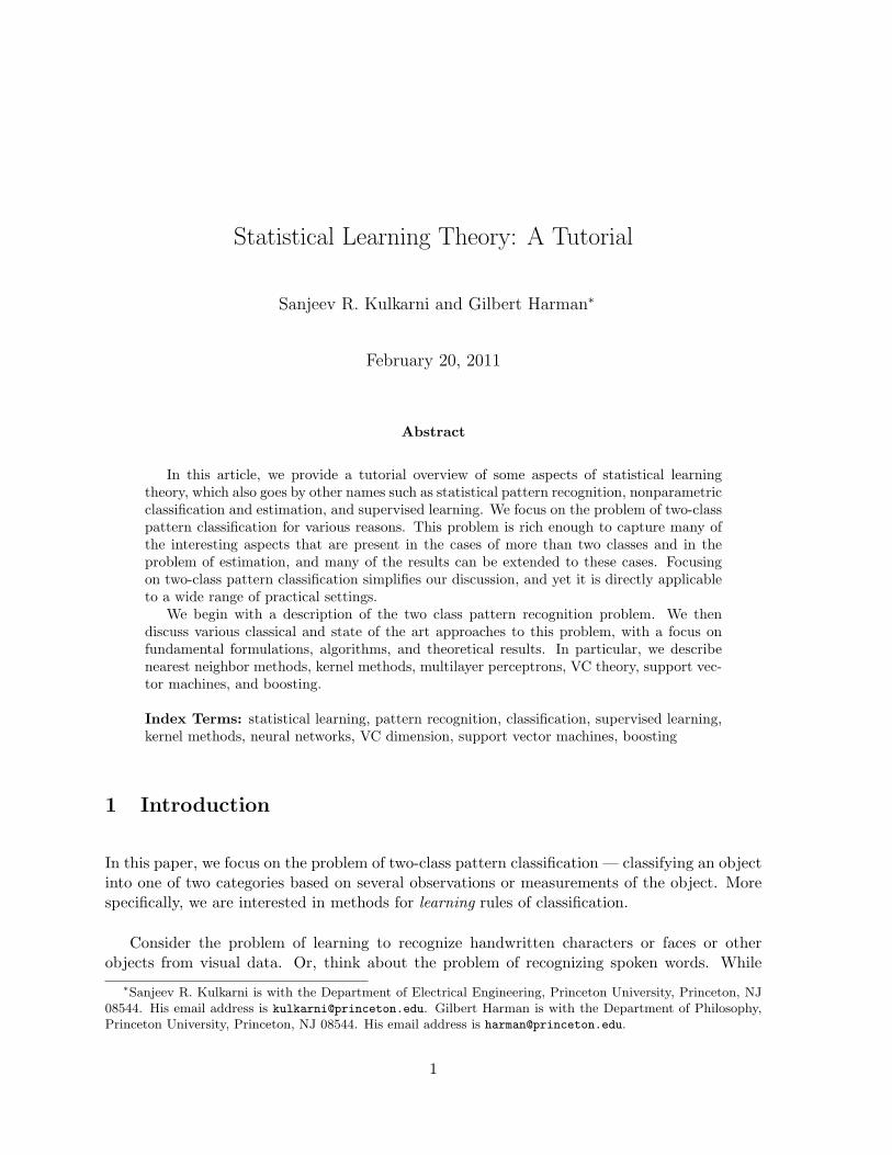
Cauchy kernel: K(x) = 1/(1 + ‖x‖d+1)Epanechnikov kernel: K(x) = (1− ‖x‖2)I‖x‖≤1.

7

Figure 3: Triangular Kernel

Figure 4: Gaussian Kernel

The positive number h is called the smoothing factor, or bandwidth, and is an importantparameter of a kernel rule. If h is small, the rule gives large relative weight to points nearx, and the decision is very “local,” while for a large h many more points are considered withfairly large weight, but these points can be farther from x. Hence, h determines the amount of“smoothing.” In choosing a value for h, one confronts a similar kind of tradeoff as in choosingthe number of neighbors using a nearest neighbor rule.

As we might expect, to get universal consistency, we need to let the smoothing factordepend on the amount of data, so we let h = hn. To make sure we get “locality” (i.e., so thatthe training examples used get closer to x), we need to have limn→∞ hn = 0. To make surethat the number of training examples used grows, we need to have limn→∞ nh

dn =∞.

These two conditions (hn → 0 and nhdn →∞) are analogous to the conditions imposed on knto get universal consistency. In addition to these two conditions, to show universal consistencywe need certain fairly mild regularity conditions on the kernel function K(·). In particular, weneed K(·) to be non-negative, and over a small neighborhood of the origin K(·) is required tobe larger than some fixed positive number b > 0. The last requirement is more technical butas a special case, it’s enough if we require that K(·) be non-increasing with distance from theorigin and have finite volume under the kernel function.

Figure 5: Cauchy Kernel

8

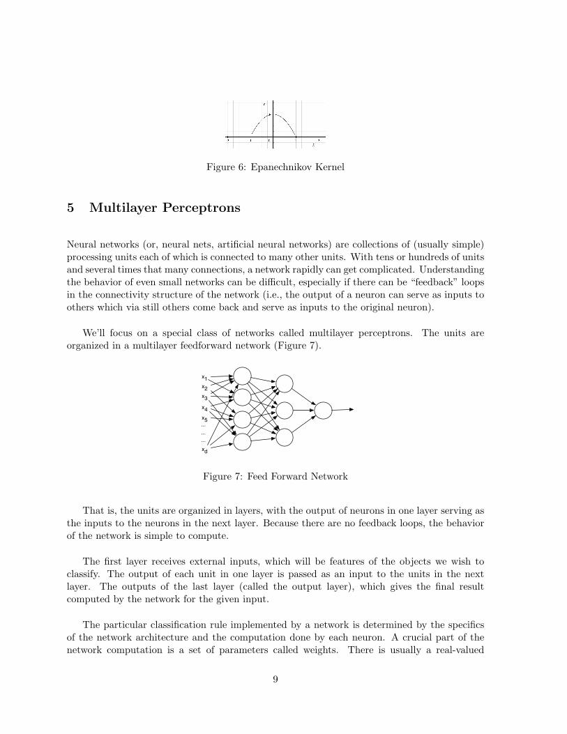
Figure 6: Epanechnikov Kernel

5 Multilayer Perceptrons

Neural networks (or, neural nets, artificial neural networks) are collections of (usually simple)processing units each of which is connected to many other units. With tens or hundreds of unitsand several times that many connections, a network rapidly can get complicated. Understandingthe behavior of even small networks can be difficult, especially if there can be “feedback” loopsin the connectivity structure of the network (i.e., the output of a neuron can serve as inputs toothers which via still others come back and serve as inputs to the original neuron).

We’ll focus on a special class of networks called multilayer perceptrons. The units areorganized in a multilayer feedforward network (Figure 7).

x1x2x3x4x5

xd

...

...

...

Figure 7: Feed Forward Network

That is, the units are organized in layers, with the output of neurons in one layer serving asthe inputs to the neurons in the next layer. Because there are no feedback loops, the behaviorof the network is simple to compute.

The first layer receives external inputs, which will be features of the objects we wish toclassify. The output of each unit in one layer is passed as an input to the units in the nextlayer. The outputs of the last layer (called the output layer), which gives the final resultcomputed by the network for the given input.

The particular classification rule implemented by a network is determined by the specificsof the network architecture and the computation done by each neuron. A crucial part of thenetwork computation is a set of parameters called weights. There is usually a real-valued

9

weight associated with each connection between units. The weights are generally consideredto be adjustable, while the rest of the network is usually thought of as fixed. Thus, we thinkof the classification rule implemented by the network as being determined by the weights, andthis classification rule can be altered if we change the weights.

To solve a given pattern recognition problem with a neural net, we need a set of weightsthat results in a good classification rule. As we discussed previously, it is difficult to directlyspecify good decision rules in most practical situations, and this is made even more difficult bythe complexity of the computation performed by the neural net. So, how should we go aboutselecting the weights of the network?

This is where learning comes in. Suppose we start with some initial set of weights. It isunlikely that the weights we start with will result in a very good classification rule. But, asbefore, we will assume we have a set of labeled examples (training data). If we use this data to“train” the network to perform well on this data, then perhaps the network will also “generalize”and provide a decision rule that works well on new data. The success of neural networks inmany practical problems is due to an efficient way to train a given network to perform well ona set of training examples, together with the fact that in many cases the resulting decision ruledoes in fact generalize well.

x1

x2

xd

...

...

...

w1

w2

wd

(1 or -1)

Figure 8: Perceptron

In a multilayer perceptron, each single unit is called a perceptron (depicted in Figure 8) thatoperates as follows. The feature vector x1, x2, . . . , xd is presented as the input so that input xiis connected to the unit with an associated weight wi.

The output a of the perceptron is given by

a = sign(x1w1 + · · ·+ xdwd)

where

sign(u) =

−1 if u < 0

1 otherwise

In general, a perceptron can have a non-zero threshold but often for convenience a threshold

10

of 0 is assumed, as we will do here. This is not restrictive since a non-zero threshold can bemimicked by a unit with a zero threshold and an extra input.

A simple learning rule, called the Perceptron Convergence Procedure, can be used for per-ceptrons to classify the well data as the perceptron can. The problem is that a perceptron canrepresent only linear decision rules (i.e., those with a hyperplane decision boundary).

+

–+

++

++

+

++

+

+

+

+

++

+

+

+

+ +++

+

+

++

+

+ +

+

+ ++

+

+–

–

–

–

––

–

–

–

––

––

– ––

–

––

–

–

––

––

–

–

–

–

––

Figure 9: Hyperplane decision rules. In R2 these are just straight lines.

Linear classifiers have been extremely well-studied, and in some applications, the best lineardecision rule may be good enough (or even optimal). But, in other problems we may need moregeneral classifiers. There may be no reason to believe that the optimal Bayes decision rule (oreven just a reasonably good rule) is linear.

Multilayer networks overcome the representation limitations of perceptrons. Perhaps sur-prisingly, with just three layers and enough units in each layer, a multilayer network can ap-proximate any decision rule. In fact, the third layer (the output layer) consists of just a singleoutput unit, so multiple units are needed only in the first and second layer.

However, due to the complexity of the network and the nonlinear relationships between theweights and the network output, a learning method for finding good weights is more difficult.

00

Figure 10: Threshold functions versus sigmoid functions

Because of this, it is very common in multilayer perceptrons to replace the threshold outputfunction of the perceptron with a “smoothed” version such as that shown on the right inFigure 10. It turns out that having the smooth function vary between 0 and 1 instead of -1and 1 simplifies things. So, for convenience, we make this change as well. A function with thisgeneral “S” shape that is differentiable, increasing, and tends to finite limits at −∞ and ∞ iscalled a sigmoid function.

11

Thus, the output of a unit is now given by

a = σ(x1w1 + · · ·+ xdwd) (8)

where the xi are the inputs to the unit, the wi are the weights, and σ(·) is a sigmoid function.One commonly used sigmoid function is

σ(y) =1

1 + e−y(9)

With a sigmoidal function small changes in one of the weights or inputs to the unit willresult in small changes to the output. This eliminates the discontinuity problem associatedwith the threshold function and allows some basic but powerful machinery from calculus andoptimization to be used to deal with the learning problem of adjusting the weights in thenetwork to perform well on the training data.

The most common learning rule for multilayer perceptrons is called backpropagation. Thisis essentially a gradient descent type of procedure that sequentially cycles through the trainingexamples and incrementally adjusts the weights in a way to as to try to reduce the errorbetween the training examples and the network output. Due to limited space, we do notprovide a detailed explanation of backpropagation here, but this can be found in a numberof books on statistical pattern recognition, learning theory, and neural networks given in thebibliography. Like all “descent” optimization algorithms, backpropagation finds only localminima. Nevertheless, it has been shown to give good results in practice, and backpropagationor its variants are the most widely used training algorithms for multilayer perceptrons.

6 Vapnik Chervonenkis Theory

Neural nets are a special case of a more general approach that fixes a collection of rules C andattempts to find a good rule from this fixed collection. In addition to the practical reasonsfor working with a fixed collection of decision rules, this perspective also leads to a fruitfulconceptual framework. The results obtained provide a characterization of the difficulty of alearning problem in terms of a measure of the “richness” of the class of decision rules.

Once the class of rules is fixed, we would like some measure of the difficulty of learning interms of the collection C. Rather than saying something about a particular method for selectinga rule from the class, we would like to say something about the inherent difficulty due to therichness of the class itself. For example, for neural nets, we would like to make statementsabout the fundamental limits of the network — not just statements about the performance ofback-propagation in particular. We would also like some measure of how much training data isrequired for learning. Vapnik-Chervonenkis theory provides results of this sort.

12

If there is only one possible decision rule in C, then “learning” is a non-issue. There isno choice but to select this one decision rule, regardless of any data observed. The issue oflearning arises when C contains many rules and we need to select a good rule from C based onthe training examples.

Each rule c ∈ C has an associated error rate R(c). A natural quantity to consider is

R∗C = minc∈C

R(c)

which is the best performance we can hope for if we are restricted to using rules from C. Ofcourse, we always have R∗C ≥ R∗. If C is rich, then R∗C may be close to the Bayes error rateR∗, but in other cases R∗C may be far from R∗.

Note that we cannot actually compute the error rates for the rules in C, since we do notknow the necessary probability distributions. Instead, we have to try to select a good rule fromC based on the data.

With a finite amount of data, it may be unreasonable to expect to always be able to find thebest rule from C. We will settle for a rule that is only approximately optimal (or approximatelycorrect). That is, we would like to select a hypothesis h from C such that the error rate R(h)of the hypothesis satisfies R(h) ≤ R∗C + ε, where ε is an accuracy parameter.

Moreover, since the training examples are random, we will require only that we produce agood hypothesis with high probability. In other words, we will require that

PR(h) ≤ R∗C + ε ≥ 1− δ

for some confidence parameter δ. This is the Probably Approximately Correct (or PAC) criterion.

Of course, we should expect that the number of examples we need to learn will depend onthe choice of ε and δ. However, we require that the number of training examples required by alearning algorithm not depend on the underlying distributions.

Specifically, we say that a class of decision rules C is PAC learnable if there is a mappingthat produces a hypotheses h ∈ C based on training examples such that for every ε, δ > 0 thereis a finite sample size m(ε, δ) such that for any distributions we have

PR(h) > R∗C + ε < δ

after seeing m(ε, δ) training examples.

There is an inherent trade-off involved in the richness of this class C. If C is too rich, thenit may be easy to find a rule that fits the data, but we won’t have confidence that performanceon the training data will be predictive of performance on new data. On the other other hand, ifC is not very rich, then perhaps no rule from C will have very good performance (even if we can

13

be confident of finding the best rule from C). Simply counting the number of rules in C is notthe right measure of complexity (or richness) of C. Instead a measure of richness should takeinto account the “expressive power” of rules in C, and this is what the notion of “shattering”and VC dimension capture.

Given a set of feature vectors x1, . . . , xn, we say that x1, . . . , xn are shattered by a class ofdecision rules C if all 2n labelings of the feature vectors x1, . . . , xn can be generated using rulesfrom C.

The Vapnik-Chervonenkis dimension (or VC dimension) of a class of decision rules C, de-noted VCdim(C), is the largest integer V such that some set of V feature vectors is shatteredby C. If arbitrarily large sets can be shattered, then VCdim(C) =∞.

Under certain mild measurability conditions, it can be shown that C is PAC learnable iffthe VC dimension of C is finite. Moreover, if V = VCdim(C) satisfies 1 ≤ V < ∞ then asample size

64ε2

(2V log

(12ε

)+ log

(4δ

))is sufficient for ε, δ learning. What is more important than the exact constants is the form ofthe bound and the fact that such a precise statement can be made. Lower bounds can also beobtained which state that ε, δ learning is not possible unless a certain number of examples areused, and the lower bounds have similar dependence on ε, δ, and V .

These results can be applied to neural networks as follows. Recall that the set of decisionrules that can be represented by a single perceptron is the set of halfspaces. If the threshold is0 the halfspaces pass through the origin, but for adjustable thresholds we get all halfspaces. Itcan be shown that in 2 dimensions, the set of halfspaces has VC dimension equal to 3. Moregenerally, the set of all halfspaces in d dimensions can be shown to have VC dimension equalto d+ 1. Thus, the learning results can be directly applied to learning using perceptrons.

Results have also been obtained for multilayer networks. Although it is quite difficult tocompute the VC dimension exactly, useful bounds have been obtained. For networks withthreshold units, one bound is that

VCdim(C) ≤ 2(d+ 1)(s) log(es)

where d is the dimension of the feature space, s is the total number of perceptrons, and e is thebase of the natural logarithm (approximately 2.718).

Similar results have been obtained for the case of sigmoidal units. In this case, the boundalso involves the maximum slope of the sigmoidal output function and the maximum allowedmagnitude for the weights.

The results involving finite VC dimension focus on the estimation error, the problem oftrying to predict which rule from C will be the best based on a set of random examples. If

14

the class of rules is too rich, then even with a large number of examples it can be difficult todistinguish those rules from C that will actually perform well on new data from those that justhappen to fit the data seen so far but have no predictive value.

In addition to the estimation error, the approximation error is also important in determiningthe overall performance of a decision rule. The approximation error sets a limit on how wellwe can do no matter how much data we receive. If we are restricted to using rules from theclass C, we can certainly do no better than the best rule from C. Once we fix a class withfinite VC dimension, we are stuck with whatever approximation error results from the classand the underlying distributions. Moreover, since the distributions are unknown, the actualapproximation error we must live with is also unknown.

If we slightly modify the PAC criterion, we can deal with certain classes that have infiniteVC dimension, and thereby address the issue of non-zero approximation errors. Consider asequence of classes C1, C2, . . . that are nested, so that C1 ⊂ C2 ⊂ · · ·. If Vi = VCdim(Ci), thenwe require Vi <∞ for all i, but we allow Vi →∞ as i→∞.

Given such a sequence of classes, we can think of VCdim(Ci) as a measure of the “complex-ity” of the class of rules Ci. We can identify the complexity of a rule with the smallest indexof a class Ci to which the rule belongs. The collection of all rules under consideration is givenby

C =∞⋃i=1

Ci.

If Vi →∞ then the class C has infinite VC dimension and so is not PAC learnable.

Nevertheless, it may turn out that we can still find good rules from C as we get more andmore data. The key idea is to allow the number of examples needed for ε, δ learning to dependon the underlying probability distributions (as well as on ε and δ), which is both an intuitiveand reasonable idea. We should expect that complicated or difficult problems will require moredata for learning, while simple problems can be learned easily with minimal data.

With this modified criterion, a hierarchy of classes C = ∪∞i=1Ci can be learned by trading offthe fit to the data against the complexity of the hypothesis. This idea is at the heart of varioustechniques that go by different names: Occam’s razor, minimum description length (MDL)principle, structural risk minimization, Akaike’s information criterion (AIC), etc. Our choiceof hypothesis should reflect some tradeoff between misfit on the data (error) and complexity.Given specific ways of measuring the error of a decision rule on the data and the complexity ofa decision rule, we can select a hypothesis by

h = argminh∈C [error(h) + complexity(h)]

Making the first term small favors choosing a hypothesis in some Ci with large i. However, ifunchecked this would result in “overfitting” and wouldn’t provide much predictive power. The

15

second term helps to control the “overfitting” problem. By striking a balance between thesetwo terms, we control the expressive power of the rules we will entertain, and also consider howwell the rules take into account the training data.

There are many choices for exactly how to carry out the misfit versus complexity tradeoff.One concrete result is as follows. Suppose the hierarchy of classes is chosen so that R∗Ci

→ R∗

as i→∞. This means that we can find rules with performance arbitrarily close to the optimalBayes decision rule as i gets sufficiently large. We select a sequence kn →∞ such that

Vkn log(n)n

→ 0 as n→∞ (10)

After seeing n examples, we select a rule hn from the class Ckn that fits the data the best. Thenit can be shown that this method is universally consistent. That is, for any distributions, asn → ∞ we have R(hn) → R∗. Hence, as we get more and more data, the performance of therule we select gets closer and closer to the Bayes error rate.

However, in general we cannot obtain uniform sample size bounds that will be guaranteeε, δ learning after some fixed number of examples. The number of examples needed will dependon the underlying distributions, and these are unknown. The performance will also dependon the choice of hierarchy of classes and the misfit/complexity tradeoff. These choices areoften a matter of art, intuition, and technical understanding of the problem domain. Thecomplexity hierarchy of the decision rules reflects the learner’s inductive bias about which rulesare considered “simple”, and how well this reflects reality has a strong effect on performance.

7 Support Vector Machines

Support Vector Machines (SVMs) provide a state-of-the-art learning method that has beenhighly successful in a variety of applications. SVMs are a special case of generalized kernelmethods, a special case of which were described in Section 4.

The origin of SVMs arises from two key ideas. The first idea is to map the feature vectors ina nonlinear way to a high (possibly infinite) dimensional space and then utilize linear classifiersin this new space. Specifically, let H denote the new feature space, and let Φ denote themapping, so that

Φ : Rd → H

For an original feature vector x ∈ Rd, the transformed feature vector is given by Φ(x). Thelabel y remains the same. Thus, the training example (xi, yi) becomes (Φ(xi), yi).

Then, we seek a hyperplane in the transformed space H that separates the transformedtraining examples (Φ(x1), y1), . . . , (Φ(xn), yn). That is, we want to find a hyperplane in thespace H so that a transformed feature vector Φ(xi) lies on one side of the hyperplane if the

16

label yi = −1, and Φ(xi) lies on the other side of the hyperplane if yi = 1. As in in Section 5,it is convenient here to assume the class labels are −1 and 1 instead of 0 and 1.

This results in nonlinear classifiers in the original space, which overcomes the representa-tional limitations of linear classifiers. However, the use of linear classifiers (in the transformedspace) lends itself to computational methods for finding a classifier that performs well on thetraining data. These computational benefits are retained while allowing a rich class of nonlinearrules.

The second key idea is to try to find hyperplanes that separate the data with a largemargin, that is a hyperplane separates the data as much as possible from among the generallyinfinitely many hyperplanes that may separate the data. While many separating hyperplanesperform equally well on the training data (in fact perfectly well if they separate the data), thegeneralization performance on new data can vary significantly.

Figure 11 shows a separable case in two dimensions with a number of separating lines.All of these separating hyperplanes perform equally well on the training data (in fact theyperform perfectly), but they might have different generalization performance. It is natural toask whether some of the separating hyperplanes are better than others in terms of their errorrate on new examples. Without some qualification, the answer is no. In a worst case sense,all hyperplanes will result in similar performance. However, it may be that the distributionsgiving rise to the worst-case performance are unusual, and that for most “typical” distributionswe might be able to do better by exploiting some properties of the training data.

--

-- -

-

---

-

++

+++

++

++

+

Figure 11: Separating Hyperlanes in Two Dimensions

It turns out that finding a hyperplane with large margin helps to provide good generalizationperformance. Intuitively, if the margin is large then the separation of the training examples isrobust to small changes in the hyperplane, and we would expect the classifier to have betterpredictive performance. This is often the case, though not in a worst-case sense. The fact thatlarge margin classifiers tend to have good generalization performance has been both justified

17

theoretically and observed in practice.

Let d+ denote the smallest distance from examples labeled 1 to the separating hyperplane,and let d− denote the smallest distance from examples labeled −1 to the separating hyperplane.The margin of the hyperplane is defined to be d+ + d−. By choosing the right orientation ofa separating hyperplane, we can make d+ + d− as large as possible. Any plane parallel to thiswill have the same value of d+ + d−.

--

-- -

-

---

-

++

+++

++

++

+

Figure 12: Large Margin Separation

In Figure 12, we show this in two dimensions. The hyperplane for which d+ = d− isshown, together with parallel hyperplanes for which either d+ = 0 or d− = 0. These last twohyperplanes will pass through one or more examples from the training data. These examplesare called the support vectors, and they are the examples that define the maximum marginhyperplane. If we move or remove the support vectors, then the maximum margin hyperplanecan change, but if we move or remove any of the other training examples, then the maximummargin hyperplane remains unchanged.

Recall that the transformed training examples are (Φ(x1), y1), . . . , (Φ(xn), yn) where Φ(xi) ∈H and yi ∈ −1, 1. The equation of a hyperplane in H can be represented in terms of a vectorw and a scalar b as

w · Φ(x) + b = 0

It turns out that w is the normal to the hyperplane and |b|/‖w‖ is the distance of the hyperplanefrom the origin.

Since there are finitely many training examples, if a hyperplane separates the training data,then each training example must be at least β away from the hyperplane for some β > 0. Thenwe can then can renormalize to require that a separating hyperplane satisfies

Φ(xi) · w + b ≥ +1 if yi = +1Φ(xi) · w + b ≤ −1 if yi = −1

18

Equivalently, we can write these conditions as

yi(Φ(xi) · w + b)− 1 ≥ 0 for i = 1, . . . , n (11)

In general, we may not be able to separate the training data with a hyperplane. However,we can still seek a hyperplane that separates the data “as much as possible” while also tryingto maximize the margin, with these objectives suitably defined. In order to carry this out, weintroduce “slack variables” ξi with ξi ≥ 0 for i = 1, . . . , n and try to satisfy

Φ(xi) · w + b ≥ +1− ξi if yi = +1Φ(xi) · w + b ≤ −1 + ξi if yi = −1

Without a constraint on the ξi, the conditions above can be satisfied trivially. We can get auseful formulation by adding a penalty term of the form C

∑i ξi, where C is some appropriate

constant.

Also, written as in Equation (11), d+ = d− = 1/‖w‖ so that

margin = d+ + d− =2‖w‖

To maximize the margin we can minimize ‖w‖, or equivalently minimize ‖w‖2.

Thus, we seek a hyperplane that solves the following optimization problem:

minimize ‖w‖2 + C∑i ξi

subject to yi(Φ(xi) · w + b)− 1 + ξi ≥ 0 for i = 1, . . . , nξi ≥ 0 for i = 1, . . . , n

Using techniques from optimization (Lagrange multipliers and considering the dual prob-lem), the maximum margin separating hyperplane can be found by solving the following opti-mization problem:

maximize∑i αi − 1

2

∑i,j αiαj yiyj (Φ(xi) · Φ(xj))

subject to∑i αiyi = 0

αi ≥ 0 for i = 1, . . . , n

This is a standard type of optimization problem called a convex quadratic programmingproblem for which there are well-known and efficient algorithms. Through solving this opti-mization, the following equations are satisfied, which provide the equation for the hyperplane:

w =n∑i=1

αiyiΦ(xi) (12)

αi(yi(w · Φ(xi) + b)− 1) = 0 for i = 1, . . . , n (13)yi(Φ(xi) · w + b)− 1 ≥ 0 for i = 1, . . . , n (14)

19

The solution to the optimization problem returns values for the αi and the ξi. From these,w can be obtained directly from the expression above in Equation (12). The scalar b can beobtained by solving Equation (13) for any i in terms of b, though a better approach is to dothis for all i and take the average of the values obtained as the choice for b.

Solving this optimization problem and obtaining the hyperplane (namely w and b) is theprocess of training. For classification, we need only check on which side of the hyperplane afeature vector x falls. That is, x is classified as 1 if

w · Φ(x) + b =n∑i=1

αiyi (Φ(xi) · Φ(x)) + b > 0

and x is classified as −1 otherwise.

For some i, it turns out that αi = 0. For these i, the corresponding example (Φ(xi), yi)does not affect the maximum margin hyperplane. For other i, we have αi > 0, and the ex-amples corresponding to these i do affect the maximum margin hyperplane. These examples(corresponding to positive αi) are the support vectors.

An important practical consideration is how to implement the transformation Φ(·). Theoriginal feature vector x is often high-dimensional itself and the transformed space is typicallyof even much higher dimension, possibly even infinite dimensional. Thus, computing Φ(xi) andΦ(x) can be very difficult.

A useful result allows us to address this issue and also provides a connection between SVMsand kernel methods discussed in Section 4. Under certain conditions the dot product Φ(xi)·Φ(x)can be replaced with a function K(xi, x) that is easy to compute. This function K(·, ·) is just akernel function, and the resulting classifier becomes a form of a general kernel classifier. Namely,a feature vector x is classified according to whether

w · Φ(x) + b =n∑i=1

αiyi (Φ(xi) · Φ(x)) + b

=n∑i=1

αiyiK(xi, x) + b

is greater than zero or less than zero.

The terms in the optimization problem used to find the αi also contain dot products of theform Φ(xi) · Φ(xj) which can be replaced with K(xi, xj).

In practice, one generally directly chooses the kernel function K, while the mapping Φ(·) andthe transformed space H are induced by the choice of K. In fact, once we specify a kernel, thetraining and classification rule can be implemented directly without the need for even knowingwhat are the corresponding Φ and H. It turns out that for a given choice of the kernel K,

20

corresponding Φ and H exist if and only if K satisfies a condition known as Mercer’s condition— i.e., for all g(x) such that

∫g(x)2 dx <∞, we have

∫K(x, z)g(x)g(z) dx dz ≥ 0.

Some common choices of kernel functions are those mentioned in Section 4. As with kernelmethods in general, the choice of the kernel function and associated parameters is an art andcan have a strong influence on classification performance.

8 Boosting

Boosting is an iterative procedure for improving the performance of any learning algorithm. Itis among the most successful learning methods available.

Boosting combines a set of “weak” classification rules to produce a “strong” compositeclassifier. A weak learning rule is one that performs strictly better than random guessing.That is, a weak learning rule and has an error rate ε = 1/2 − γ for some γ > 0. Because ofcomputational or other considerations, it might be easy to produce a weak learning rule, eventhough finding a good rule may be difficult. This is where boosting comes into play. If we havean algorithm that given training data can find a weak classifier, then boosting can be used toproduce a new classifier with much better performance.

Boosting proceeds in a series of rounds. In each round, a weak rule is produced by runningsome basic learning algorithm using a different weighting of the training examples. Startingwith equal weighting in the first round, the weighting of the training examples is updated aftereach round to place more weight on those training examples that are misclassified by the currentweak hypothesis just produced and less weight on those that are correctly classified. This forcesthe weak learner to concentrate in the next round on these hard-to-classify examples.

Specifically, let Dt(·) denote the distribution on the training examples at round t, so thatDt(i) is the probability (or weight) that we assign to the i-th training example. At stage t,the goal of the weak learning algorithm will be produce a hypothesis ht(·) that attempts tominimize the weighted error, εt defined by

εt =n∑i=1

Dt(i)Iht(xi)6=yi (15)

εt as the probability of error of the classifier ht(·), where the probability is computed withrespect to the distribution Dt(·). To compute ht, “new” examples can be generated by drawingexamples from the training data (xi, yi) according to these probabilities, and then train thelearning algorithm on this set of “new” examples. Or, if possible, we can simply apply thelearning algorithm with the objective of minimizing the weighted training error.

After a number of rounds, a final classification rule is produced via a weighted sum of

21

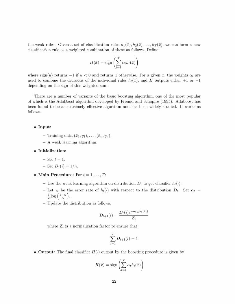
the weak rules. Given a set of classification rules h1(x), h2(x), . . . , hT (x), we can form a newclassification rule as a weighted combination of these as follows. Define

H(x) = sign

(T∑t=1

αtht(x)

)

where sign(u) returns −1 if u < 0 and returns 1 otherwise. For a given x, the weights αt areused to combine the decisions of the individual rules ht(x), and H outputs either +1 or −1depending on the sign of this weighted sum.

There are a number of variants of the basic boosting algorithm, one of the most popularof which is the AdaBoost algorithm developed by Freund and Schapire (1995). Adaboost hasbeen found to be an extremely effective algorithm and has been widely studied. It works asfollows.

• Input:

– Training data (x1, y1), . . . , (xn, yn).

– A weak learning algorithm.

• Initialization:

– Set t = 1.

– Set D1(i) = 1/n.

• Main Procedure: For t = 1, . . . , T :

– Use the weak learning algorithm on distribution Dt to get classifier ht(·).– Let εt be the error rate of ht(·) with respect to the distribution Dt. Set αt =

12 log

(1−εtεt

).

– Update the distribution as follows:

Dt+1(i) =Dt(i)e−αtyiht(xi)

Zt

where Zt is a normalization factor to ensure that

T∑t=1

Dt+1(i) = 1

• Output: The final classifier H(·) output by the boosting procedure is given by

H(x) = sign

(T∑t=1

αtht(x)

)

22

To discuss the performance of Adaboost, let γt = 1/2 − εt. Since εt < 1/2, γt > 0 and isthe amount by which ht performs better than random guessing on the training data (weightedaccording to Dt).

It can be shown that the training error of the final classifier H produced by AdaBoost isbounded as follows:

1n

n∑i=1

IH(xi)6=yi ≤ e−2∑T

t=1γ2

t . (16)

The bound on the right hand side of Equation (16) gets smaller with every round, and if γt ≥ γfor some γ > 0 then

e−2∑T

t=1γ2

t ≤ e−2∑T

t=1γ2

= e−2Tγ2

so that the training error approaches zero exponentially fast in the number of rounds T .

Boosting algorithms prior to AdaBoost satisfied similar bounds on the training error butrequired knowledge of γ, which can be hard to obtain. The beauty of AdaBoost is that itadapts naturally to the error rates of ht so that knowledge of γ is not required (hence the nameAdaBoost, short for Adaptive Boosting).

While the performance on the training data is reassuring, for a learning method to bevaluable we are interested in the generalization error as opposed to the training error. Thegeneralization performance of H, denoted R(H), is given by

R(H) = PH(x) 6= y

and is the probability that H misclassifies a new randomly drawn example.

Using VC theory, it can be shown that with high probability the error rate after T roundsof boosting is bounded as follows:

R(H) ≤ 1n

n∑i=1

IH(xi)6=yi +O

√TV

n

. (17)

The problem with this bound is that it increases with the number of rounds T , suggesting thatboosting will tend to overfit the training data as we run it for more rounds. However, whilesometimes overfitting is observed, in many cases the generalization error continues to decreaseas the number of rounds increases, and this can happen even after the error on the trainingdata is zero. Explanations for this have been provided in terms of the margins of the classifier.

Here we use a slightly different way to measure the margin than was used in Section 7.Define the margin of the example (xi, yi) as

margin(xi, yi) =yi∑Tt=1 αtht(xi)∑Tt=1 αt

(18)

23

The margin of (xi, yi) is always between −1 and +1 and is positive if and only if H classifies(xi, yi) correctly. In a sense, the margin measures the confidence in our classification of (xi, yi).

It can be shown that for any θ > 0, with high probability we have

R(H) ≤ 1n

n∑i=1

Imargin(xi,yi)≤θ +O

√ V

nθ2

. (19)

An important feature of this bound is that it does not depend on T . This helps explainthe empirical observation that running boosting for many rounds often does not increase thegeneralization error.

References

[1] M. Anthony and P.L. Bartlett, Neural Network Learning: Theoretical Foundations, Cam-bridge University Press, 1999.

[2] C. Bishop, Pattern Recognition and Machine Learning, Springer, New York, 2006.

[3] C.J.C. Burges, “A Tutorial on Support Vector Machines for Pattern Recognition,” DataMining and Knowledge Discovery, Vol. 2, pp.121167, 1998.

[4] N. Cristianini and J. Shawe-Taylor, An Introduction to Support Vector Machines, Cam-bridge University Press, 2000.

[5] P.R. Devijver and J. Kittler, Pattern Recognition: A Statistical Approach, Prentice-Hall,1982.

[6] L. Devroye, L. Gyorfi, G. Lugosi, A Probabilistic Theory of Pattern Recognition, SpringerVerlag, New York, 1996.

[7] R.O. Duda, P.E. Hart, and D.G. Stork, Pattern Classification, Second Edition, Wiley, NewYork, 2001.

[8] K. Fukunaga, Introduction to Statistical Pattern Recognition, Second Edition, AcademicPress, 1990.

[9] G. Harman and S.R. Kulkarni, An Elementary Introduction to Statistical Learning Theory,Wiley, 2011.

[10] G. Harman and S.R. Kulkarni, Reliable Reasoning: Induction and Statistical LearningTheory, MIT Press, 2007.

[11] T. Hastie, R. Tibshirani, J. Friedman, The Elements of Statistical Learning: Data Mining,Inference, and Prediction, Second Edition, Springer, 2009.

24

[12] S. Haykin, Neural Networks: A Comprehensive Foundation, Macmillan Publishing Com-pany, 1994.

[13] M.J. Kearns and U.V. Vazirani, An Introduction to Computational Learning Theory, MITPress, 1994.

[14] S.R. Kulkarni, G. Lugosi, and Venkatesh, S., “Learning Pattern Classification – A Survey,”IEEE Transactions on Information Theory, Vol. 44, No. 6, pp. 2178-2206, Oct., 1998.

[15] D.J.C. MacKay, Information Theory, Inference, & Learning Algorithms, Cambridge Uni-versity Press, 2002.

[16] T. Mitchell, Machine learning, McGraw-Hill, 1997.

[17] S. Russell and P. Norvig P, Artificial Intelligence: A Modern Approach, Third Edition,Prentice-Hall, 2011.

[18] R.J. Schalkoff, Pattern Recognition: Statistical, Structural, and Neural Approaches, Wiley,1992.

[19] R.E. Schapire, “A brief introduction to boosting,” Proceedings of the Sixteenth Interna-tional Joint Conference on Artificial Intelligence, 1999.

[20] J. Shawe-Taylor and N. Cristianini, Kernel Methods for Pattern Analysis, Cambridge Uni-versity Press, 2004.

[21] S. Theodoridis and K. Koutroumbas, Pattern Recognition, Fourth Edition, Academic Press,2008.

[22] V.N. Vapnik, The Nature of Statistical Learning Theory, Springer-Verlag, New York, 1996.

[23] V. Vapnik, Statistical Learning Theory, Wiley-Interscience, New York, 1998.

[24] M. Vidyasagar, A Theory of Learning and Generalization, Springer-Verlag, 1997.

25