statistical learning theory - statistics...

Statistical Learning TheoryMachine Learning Summer School, Kyoto, Japan

Alexander (Sasha) Rakhlin

University of Pennsylvania, The Wharton SchoolPenn Research in Machine Learning (PRiML)

August 27-28, 2012

1 / 130

References

Parts of these lectures are based on

▸ O. Bousquet, S. Boucheron, G. Lugosi:“Introduction to Statistical Learning Theory”, 2004.

▸ MLSS notes by O. Bousquet

▸ S. Mendelson: “A Few Notes on Statistical Learning Theory”

▸ Lecture notes by S. Shalev-Shwartz

▸ Lecture notes (S. R. and K. Sridharan)http://stat.wharton.upenn.edu/~rakhlin/courses/stat928/stat928_notes.pdf

Prerequisites: a basic familiarity with Probability is assumed.

2 / 130

http://stat.wharton.upenn.edu/~rakhlin/courses/stat928/stat928_notes.pdf

Outline

Introduction

Statistical Learning TheoryThe Setting of SLTConsistency, No Free Lunch Theorems, Bias-Variance TradeoffTools from Probability, Empirical ProcessesFrom Finite to Infinite ClassesUniform Convergence, Symmetrization, and Rademacher ComplexityLarge Margin Theory for ClassificationProperties of Rademacher ComplexityCovering Numbers and Scale-Sensitive DimensionsFaster RatesModel Selection

Sequential Prediction / Online LearningMotivationSupervised LearningOnline Convex and Linear OptimizationOnline-to-Batch Conversion, SVM optimization

3 / 130

Example #1: Handwritten Digit Recognition

Imagine you are asked to write a computer program that recognizes postalcodes on envelopes. You observe the huge amount of variation andambiguity in the data:

One can try to hard-code all the possibilities, but likely to fail. It would benice if a program looked at a large corpus of data and learned thedistinctions!

This picture of MNIST dataset was yanked from http://www.heikohoffmann.de/htmlthesis/node144.html4 / 130

Example #1: Handwritten Digit Recognition

Need to represent data in the computer. Pixel intensities is one possibility,but not necessarily the best one. Feature representation:

1.15.36.22.92.3...feature map

We also need to specify the “label” of this example: “3”. The labeledexample is then

1.15.36.22.92.3...( ,3

(After looking at many of these examples, we want the program to predictthe label of the next hand-written digit.

5 / 130

Example #2: Predict Topic of a News ArticleYou would like to automatically collect news stories from the web anddisplay them to the reader in the best possible way. You would like togroup or filter these articles by topic. Hard-coding possible topics forarticles is a daunting task!

Representation in the computer:

010250110...

This is a bag-of-words representation. If “1” stands for the category“politics”, then this example can be represented as

010250110...

( ,1

(

After looking at many of such examples, we would like the program topredict the topic of a new article.

6 / 130

Why Machine Learning?

▸ Impossible to hard-code all the knowledge into a computer program.

▸ The systems need to be adaptive to the changes in the environment.

Examples:

▸ Computer vision: face detection, face recognition

▸ Audio: voice recognition, parsing

▸ Text: document topics, translation

▸ Ad placement on web pages

▸ Movie recommendations

▸ Email spam detection

7 / 130

Machine Learning

(Human) learning is the process of acquiring knowledge or skill.

Quite vague. How can we build a mathematical theory for something soimprecise?

Machine Learning is concerned with the design and analysis of algorithmsthat improve performance after observing data.

That is, the acquired knowledge comes from data.

We need to make mathematically precise the following terms: performance,improve, data.

8 / 130

Learning from Examples

How is it possible to conclude something general from specific examples?

Learning is inherently an ill-posed problem, as there are many alternativesthat could be consistent with the observed examples.

Learning can be seen as the process of induction (as opposed to deduction):“extrapolating” from examples.

Prior knowledge is how we make the problem well-posed.

Memorization is not learning, not induction. Our theory should make thisapparent.

Very important to delineate assumptions. Then we will be able to provemathematically that certain learning algorithms perform well.

9 / 130

DataSpace of inputs (or, predictors): X

▷ e.g. x ∈ X ⊂ {0, 1, . . . , 216}64 is a string of pixel intensities in an 8 × 8image.

▷ e.g. x ∈ X ⊂ R33,000 is a set of gene expression levels.

x1 = x2 = . . .

x1 = x2 = . . .

x1 =

5

1

22...

x2 =

...

1

0

17

# cigarettes/day

# drinks/day

BMI

10 / 130

Data

Sometimes the space X is uniquely defined for the problem. In other cases,such as in vision/text/audio applications, many possibilities exist, and agood feature representation is key to obtaining good performance.

This important part of machine learning applications will not be discussedin this lecture, and we will assume that X has been chosen by thepractitioner.

11 / 130

Data

Space of outputs (or, responses): Y

▷ e.g. y ∈ Y = {0, 1} is a binary label (1 = “cat”)

▷ e.g. y ∈ Y = [0, 200] is life expectancy

A pair (x,y) is a labeled example.

▷ e.g. (x,y) is an example of an image with a label y = 1, which stands forthe presence of a face in the image x

Dataset (or training data): examples {(x1,y1), . . . , (xn,yn)}

▷ e.g. a collection of images labeled according to the presence or absenceof a face

12 / 130

The Multitude of Learning Frameworks

Presence/absence of labeled data:

▸ Supervised Learning: {(x1,y1), . . . , (xn,yn)}▸ Unsupervised Learning: {x1, . . . ,xn}▸ Semi-supervised Learning: a mix of the above

This distinction is important, as labels are often difficult or expensive toobtain (e.g. can collect a large corpus of emails, but which ones are spam?)

Types of labels:

▸ Binary Classification / Pattern Recognition: Y = {0, 1}▸ Multiclass: Y = {0, . . . ,K}▸ Regression: Y ⊆ R▸ Structure prediction: Y is a set of complex objects (graphs,

translations)

13 / 130

The Multitude of Learning Frameworks

Problems also differ in the protocol for obtaining data:

▸ Passive

▸ Active

and in assumptions on data:

▸ Batch (typically i.i.d.)

▸ Online (i.i.d. or worst-case or some stochastic process)

Even more involved: Reinforcement Learning and other frameworks.

14 / 130

Why Theory?

“... theory is the first term in the Taylor series of practice”– Thomas M. Cover, “1990 Shannon Lecture”

Theory and Practice should go hand-in-hand.

Boosting, Support Vector Machines – came from theoretical considerations.

Sometimes, theory is suggesting practical methods, sometimes practicecomes ahead and theory tries to catch up and explain the performance.

15 / 130

This tutorial

First 2/3 of the tutorial: we will study the problem of supervised learning(with a focus on binary classification) with an i.i.d. assumption on the data.

The last 1/3 of the tutorial: we will turn to online learning without thei.i.d. assumption.

16 / 130

Outline

Introduction



17 / 130

Outline

Introduction



18 / 130

Statistical Learning Theory

The variable x is related to y, and we would like to learn this relationshipfrom data.

The relationship is encapsulated by a distribution P on X ×Y.

Example: x = [weight, blood glucose, . . .] and y is the risk of diabetes. Weassume there is a relationship between x and y: it is less likely to seecertain x co-occur with “low risk” and unlikely to see some other x co-occurwith “high risk”. This relationship is encapsulated by P(x,y).

This is an assumption about the population of all (x,y). However, what wesee is a sample.

19 / 130


Data denoted by {(x1,y1), . . . , (xn,yn)}, where n is the sample size.

The distribution P is unknown to us (otherwise, there is no learning to bedone).

The observed data are sampled independently from P (the i.i.d.assumption)

It is often helpful to write P = Px ×Py∣x. The distribution Px on the inputs iscalled the marginal distribution, while Py∣x is the conditional distribution.

20 / 130


Upon observing the training data {(x1,y1), . . . , (xn,yn)}, the learner isasked to summarize what she had learned about the relationship between xand y.

The learner’s summary takes the form of a function fn ∶ X ↦ Y. The hatindicates that this function depends on the training data.

Learning algorithm: a mapping {(x1,y1), . . . , (xn,yn)}z→ fn.

The quality of the learned relationship is given by comparing the responsefn(x) to y for a pair (x,y) independently drawn from the same distributionP:

E(x,y)`(fn(x),y)where ` ∶ Y ×Y ↦ R is a loss function. This is our measure of performance.

21 / 130

Loss Functions

▸ Indicator loss (classification): `(y,y ′) = I{y≠y ′}

▸ Square loss: `(y,y ′) = (y − y ′)2

▸ Absolute loss: `(y,y ′) = ∣y − y ′∣

22 / 130

Examples

Probably the simplest learning algorithm that you are probably familiarwith is linear least squares:

Given (x1,y1), . . . , (xn,yn), let

β = arg minβ∈Rd

1

n

n

∑i=1

(yi − ⟨β,xi⟩)2

and definefn(x) = ⟨β,x⟩

Another basic method is regularized least squares:

β = arg minβ∈Rd

1

n

n

∑i=1

(yi − ⟨β,xi⟩)2 + λ∥β∥2

23 / 130

Methods vs Problems

Algorithms fn Distributions P

24 / 130

Expected Loss and Empirical Loss

The expected loss of any function f ∶ X ↦ Y is

L(f) = E`(f(x),y)

Since P is unknown, we cannot calculate L(f).

However, we can calculate the empirical loss of f ∶ X ↦ Y

L(f) = 1

n

n

∑i=1

`(f(xi),yi)

25 / 130

... again, what is random here?

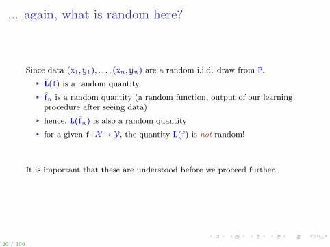
Since data (x1,y1), . . . , (xn,yn) are a random i.i.d. draw from P,

▸ L(f) is a random quantity

▸ fn is a random quantity (a random function, output of our learningprocedure after seeing data)

▸ hence, L(fn) is also a random quantity

▸ for a given f ∶ X → Y, the quantity L(f) is not random!

It is important that these are understood before we proceed further.

26 / 130

The Gold Standard

Within the framework we set up, the smallest expected loss is achieved bythe Bayes optimal function

f∗ = arg min

fL(f)

where the minimization is over all (measurable) prediction rules f ∶ X ↦ Y.

The value of the lowest expected loss is called the Bayes error:

L(f∗) = inffL(f)

Of course, we cannot calculate any of these quantities since P is unknown.

27 / 130

Bayes Optimal Function

Bayes optimal function f∗ takes on the following forms in these twoparticular cases:

▸ Binary classification (Y = {0, 1}) with the indicator loss:

f∗(x) = I{η(x)≥1/2}, where η(x) = E[Y∣X = x]

0

1

⌘(x)

▸ Regression (Y = R) with squared loss:

f∗(x) = η(x), where η(x) = E[Y∣X = x]

28 / 130

The big question: is there a way to construct a learning algorithm with aguarantee that

L(fn) − L(f∗)is small for large enough sample size n?

29 / 130

Outline

Introduction



30 / 130

Consistency

An algorithm that ensures

limn→∞

L(fn) = L(f∗) almost surely

is called consistent. Consistency ensures that our algorithm is approachingthe best possible prediction performance as the sample size increases.

The good news: consistency is possible to achieve.

▸ easy if X is a finite or countable set

▸ not too hard if X is infinite, and the underlying relationship between xand y is “continuous”

31 / 130

The bad news...

In general, we cannot prove anything “interesting” about L(fn) − L(f∗),unless we make further assumptions (incorporate prior knowledge).

What do we mean by “nothing interesting”? This is the subject of theso-called “No Free Lunch” Theorems. Unless we posit further assumptions,

▸ For any algorithm fn, any n and any ε > 0, there exists a distributionP such that L(f∗) = 0 and

EL(fn) ≥1

2− ε

▸ For any algorithm fn, and any sequence an that converges to 0, thereexists a probability distribution P such that L(f∗) = 0 and for all n

EL(fn) ≥ an

Reference: (Devroye, Gyorfi, Lugosi: A Probabilistic Theory of Pattern Recognition),

(Bousquet, Boucheron, Lugosi, 2004)

32 / 130

is this really “bad news”?

Not really. We always have some domain knowledge.

Two ways of incorporating prior knowledge:

▸ Direct way: assume that the distribution P is not arbitrary (also knownas a modeling approach, generative approach, statistical modeling)

▸ Indirect way: redefine the goal to perform as well as a reference set Fof predictors:

L(fn) − inff∈F

L(f)

This is known as a discriminative approach. F encapsulates ourinductive bias.

33 / 130

Pros/Cons of the two approaches

Pros of the discriminative approach: we never assume that P takes someparticular form, but we rather put our prior knowledge into “what are thetypes of predictors that will do well”. Cons: cannot really interpret fn.

Pros of the generative approach: can estimate the model / parameters ofthe distribution (inference). Cons: it is not clear what the analysis says ifthe assumption is actually violated.

Both approaches have their advantages. A machine learning researcher orpractitioner should ideally know both and should understand theirstrengths and weaknesses.

In this tutorial we only focus on the discriminative approach.

34 / 130

Example: Linear Discriminant Analysis

Consider the classification problem with Y = {0, 1}. Suppose theclass-conditional densities are multivariate Gaussian with the samecovariance Σ = I:

p(x∣y = 0) = (2π)−k/2

exp{−1

2∥x −µ0∥

2}

andp(x∣y = 1) = (2π)

−k/2exp{−

1

2∥x −µ1∥

2}

The “best” (Bayes) classifier is f∗ = I{P(y=1∣x)≥1/2} which corresponds to thehalf-space defined by the decision boundary p(x∣y = 1) ≥ p(x∣y = 0). Thisboundary is linear.

35 / 130

Example: Linear Discriminant Analysis

The (linear) optimal decision boundary comes from our generativeassumption on the form of the underlying distribution.

Alternatively, we could have indirectly postulated that we will be lookingfor a linear discriminant between the two classes, without makingdistributional assumptions. Such linear discriminant (classification)functions are

I{⟨w,x⟩≥b}

for a unit-norm w and some bias b ∈ R.

Quadratic Discriminant Analysis: If unequal correlation matrices Σ1 and Σ2

are assumed, the resulting boundary is quadratic. We can then defineclassification function by

I{q(x)≥0}

where q(x) is a quadratic function.

36 / 130

Bias-Variance TradeoffHow do we choose the inductive bias F?

L(fn) − L(f∗) = L(fn) − inff∈F

L(f)´¹¹¹¹¹¹¹¹¹¹¹¹¹¹¹¹¹¹¹¹¹¹¹¹¹¹¹¹¹¹¹¹¹¹¹¹¹¹¹¹¹¹¹¸¹¹¹¹¹¹¹¹¹¹¹¹¹¹¹¹¹¹¹¹¹¹¹¹¹¹¹¹¹¹¹¹¹¹¹¹¹¹¹¹¹¹¹¶

Estimation Error

+ inff∈F

L(f) − L(f∗)´¹¹¹¹¹¹¹¹¹¹¹¹¹¹¹¹¹¹¹¹¹¹¹¹¹¹¹¹¹¹¹¹¹¹¹¹¹¹¹¹¹¹¸¹¹¹¹¹¹¹¹¹¹¹¹¹¹¹¹¹¹¹¹¹¹¹¹¹¹¹¹¹¹¹¹¹¹¹¹¹¹¹¹¹¶

Approximation Error

F

fn f⇤fF

Clearly, the two terms are at odds with each other:

▸ Making F larger means smaller approximation error but (as we willsee) larger estimation error

▸ Taking a larger sample n means smaller estimation error and has noeffect on the approximation error.

▸ Thus, it makes sense to trade off size of F and n. This is calledStructural Risk Minimization, or Method of Sieves, or Model Selection.

37 / 130

Bias-Variance Tradeoff

We will only focus on the estimation error, yet the ideas we develop willmake it possible to read about model selection on your own.

Note: if we guessed correctly and f∗ ∈ F , then

L(fn) − L(f∗) = L(fn) − inff∈F

L(f)

For a particular problem, one hopes that prior knowledge about the problemcan ensure that the approximation error inff∈F L(f) − L(f∗) is small.

38 / 130

Occam’s Razor

Occam’s Razor is often quoted as a principle for choosing the simplesttheory or explanation out of the possible ones.

However, this is a rather philosophical argument since simplicity is notuniquely defined. We will discuss this issue later.

What we will do is to try to understand “complexity” when it comes tobehavior of certain stochastic processes. Such a question will bewell-defined mathematically.

39 / 130

Looking Ahead

So far: represented prior knowledge by means of the class F .

Looking forward, we can find an algorithm that, after looking at a datasetof size n, produces fn such that

L(fn) − inff∈F

L(f)

decreases (in a certain sense which we will make precise) at a non-trivialrate which depends on “richness” of F .

This will give a sample complexity guarantee: how many samples areneeded to make the error smaller than a desired accuracy.

40 / 130

Outline

Introduction



41 / 130

Types of Bounds

In expectation vs in probability (control the mean vs control the tails):

E{L(fn) − inff∈F

L(f)} < ψ(n) vs P (L(fn) − inff∈F

L(f) ≥ ε) < ψ(n,ε)

The in-probability bound can be inverted as

P (L(fn) − inff∈F

L(f) ≥ φ(δ,n)) < δ

by setting δ ∶= ψ(ε,n) and solving for ε.

In this lecture, we are after the function φ(δ,n). We will call it “the rate”.

“With high probability” typically means logarithmic dependence of φ(δ,n)on 1/δ. Very desirable: the bound grows only modestly even for highconfidence bounds.

42 / 130

Sample Complexity

Sample complexity is the sample size required by the algorithm fn toguarantee L(fn) − inff∈F L(f) ≤ ε with probability at least 1 − δ. Of course,we just need to invert a bound


L(f) ≥ φ(δ,n)) < δ

by setting ε ∶= φ(δ,n) and solving for n. In other words, n(ε, δ) is samplecomplexity of the algorithm fn if


L(f) ≥ ε) ≤ δ

as soon as n ≥ n(ε, δ).

Hence, “rate” can be translated into “sample complexity” and vice versa.

Easy to remember: rate O(1/√n) means O(1/ε2) sample complexity,

whereas rate O(1/n) is a smaller O(1/ε) sample complexity.

43 / 130

Types of BoundsOther distinctions to keep in mind: We can ask for bounds (either inexpectation or in probability) on the following random variables:

L(fn) − L(f∗) (A)

L(fn) − inff∈F

L(f) (B)

L(fn) − L(fn) (C)

supf∈F

{L(f) − L(f)} (D)

supf∈F

{L(f) − L(f) − penn(f)} (E)

Let’s make sure we understand the differences between these randomquantities!

44 / 130

Types of Bounds

Upper bounds on (D) and (E) are used as tools for achieving the otherbounds. Let’s see why.

Obviously, for any algorithm that outputs fn ∈ F ,

L(fn) − L(fn) ≤ supf∈F

{L(f) − L(f)}

and so a bound on (D) implies a bound on (C).

How about a bound on (B)? Is it implied by (C) or (D)? It depends onwhat the algorithm does!

Denote fF = arg minf∈F L(f). Suppose (D) is small. It then makes sense toask the learning algorithm to minimize or (approximately minimize) theempirical error (why?)

45 / 130

Canonical Algorithms

Empirical Risk Minimization (ERM) algorithm:

fn = arg minf∈F

L(f)

Regularized Empirical Risk Minimization algorithm:

fn = arg minf∈F

L(f) + penn(f)

We will deal with the regularized ERM a bit later. For now, let’s focus onERM.

Remark: to actually compute f ∈ F minimizing the above objectives, oneneeds to employ some optimization methods. In practice, the objectivemight be optimized only approximately.

46 / 130

Performance of ERM

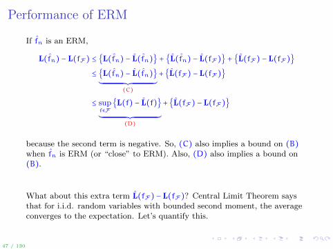
If fn is an ERM,

L(fn) − L(fF) ≤ {L(fn) − L(fn)} + {L(fn) − L(fF)} + {L(fF) − L(fF)}≤ {L(fn) − L(fn)}´¹¹¹¹¹¹¹¹¹¹¹¹¹¹¹¹¹¹¹¹¹¹¹¹¹¹¹¹¹¹¹¹¹¹¹¹¹¹¹¹¹¹¹¹¸¹¹¹¹¹¹¹¹¹¹¹¹¹¹¹¹¹¹¹¹¹¹¹¹¹¹¹¹¹¹¹¹¹¹¹¹¹¹¹¹¹¹¹¹¶

(C)

+{L(fF) − L(fF)}

≤ supf∈F

{L(f) − L(f)}´¹¹¹¹¹¹¹¹¹¹¹¹¹¹¹¹¹¹¹¹¹¹¹¹¹¹¹¹¹¹¹¹¹¹¹¹¹¹¹¹¹¹¹¹¹¹¹¹¹¸¹¹¹¹¹¹¹¹¹¹¹¹¹¹¹¹¹¹¹¹¹¹¹¹¹¹¹¹¹¹¹¹¹¹¹¹¹¹¹¹¹¹¹¹¹¹¹¹¹¶

(D)

+{L(fF) − L(fF)}

because the second term is negative. So, (C) also implies a bound on (B)when fn is ERM (or “close” to ERM). Also, (D) also implies a bound on(B).

What about this extra term L(fF) − L(fF)? Central Limit Theorem saysthat for i.i.d. random variables with bounded second moment, the averageconverges to the expectation. Let’s quantify this.

47 / 130

Hoeffding Inequality

Let W,W1, . . . ,Wn be i.i.d. such that P (a ≤W ≤ b) = 1. Then

P (EW − 1

n

n

∑i=1

Wi > ε) ≤ exp(− 2nε2

(b − a)2)

and

P ( 1

n

n

∑i=1

Wi − EW > ε) ≤ exp(− 2nε2

(b − a)2)

Let Wi = `(fF(xi),yi). Clearly, W1, . . . ,Wi are i.i.d. Then,

P (∣L(fF) − L(fF)∣ > ε) ≤ 2 exp(− 2nε2

(b − a)2)

assuming a ≤ `(fF(x),y) ≤ b for all x ∈ X ,y ∈ Y.

48 / 130

Wait, Are We Done?

Can’t we conclude directly that (C) is small? That is,

P (E`(fn(x),y) −1

n

n

∑i=1

`(fn(xi),yi) > ε) ≤ 2 exp(− 2nε2

(b − a)2) ?

No! The random variables `(fn(xi),yi) are not necessarily independent andit is possible that

E`(fn(x),y) = EW ≠ E`(fn(xi),yi) = EWi

The expected loss is “out of sample performance” while the second term is“in sample”.

We say that `(fn(xi),yi) is a biased estimate of E`(fn(x),y).

How bad can this bias be?

49 / 130

Example

▸ X = [0, 1], Y = {0, 1}▸ `(f(Xi),Yi) = I{f(Xi)≠Yi}

▸ distribution P = Px × Py∣x with Px = Unif[0, 1] and Py∣x = δy=1

▸ function class

F = ∪n∈N{f = fS ∶ S ⊂ X , ∣S∣ = n, fS(x) = I{x∈S}}

0

1

1

ERM fn memorizes (perfectly fits) the data, but has no ability togeneralize. Observe that

0 = E`(fn(xi),yi) ≠ E`(fn(x),y) = 1

This phenomenon is called overfitting.

50 / 130

Example

Not only is (C) large in this example. Also, uniform deviations (D) do notconverge to zero.

For any n ∈ N and any (x1,y1), . . . , (xn,yn) ∼ P

supf∈F

{Ex,y`(f(x),y) −1

n

n

∑i=1

`(f(xi),yi)} = 1

Where do we go from here? Two approaches:

1. understand how to upper bound uniform deviations (D)2. find properties of algorithms that limit in some way the bias of`(fn(xi),yi). Stability and compression are two such approaches.

51 / 130

Uniform Deviations

We first focus on understanding

supf∈F

{Ex,y`(f(x),y) −1

n

n

∑i=1

`(f(xi),yi)}

If F = {f0} consists of a single function, then clearly

supf∈F

{E`(f(x),y) − 1

n

n

∑i=1

`(f(xi),yi)} = {E`(f0(x),y) −1

n

n

∑i=1

`(f0(xi),yi)}

This quantity is OP(1/√n) by Hoeffding’s inequality, assuming

a ≤ `(f0(x),y) ≤ b.

Moral: for “simple” classes F the uniform deviations (D) can be boundedwhile for “rich” classes not. We will see how far we can push the size of F .

52 / 130

A bit of notation to simplify things...

To ease the notation,

▸ Let zi = (xi,yi) so that the training data is {z1, . . . , zn}▸ g(z) = `(f(x),y) for z = (x,y)▸ Loss class G = {g ∶ g(z) = `(f(x),y)} = ` ○F▸ gn = `(fn(⋅), ⋅), gG = `(fF(⋅), ⋅)▸ g∗ = arg ming Eg(z) = `(f∗(⋅), ⋅) is Bayes optimal (loss) function

We can now work with the set G, but keep in mind that each g ∈ Gcorresponds to an f ∈ F :

g ∈ G ←→ f ∈ F

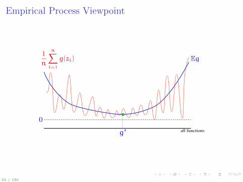
Once again, the quantity of interest is

supg∈G

{Eg(z) − 1

n

n

∑i=1

g(zi)}

On the next slide, we visualize deviations Eg(z) − 1n ∑

ni=1 g(zi) for all

possible functions g and discuss all the concepts introduces so far.

53 / 130

Empirical Process Viewpoint

g⇤0

Eg

all functions

g⇤0

Eg

all functions

1

n

nX

i=1

g(zi)

g⇤0

Eg

all functions

1

n

nX

i=1

g(zi)

g⇤0

Eg

all functions

1

n

nX

i=1

g(zi)

gn g⇤0

1

n

nX

i=1

g(zi)

gn

G

g⇤0

Eg

all functions

1

n

nX

i=1

g(zi)G

g⇤0

Eg

all functions

1

n

nX

i=1

g(zi)

gG gn

G

g⇤0

Eg

all functions

1

n

nX

i=1

g(zi)

54 / 130


g⇤0

Eg

all functionsg⇤0

Eg

all functions

1

n

nX

i=1

g(zi)

g⇤0

Eg

all functions

1

n

nX

i=1

g(zi)

g⇤0

Eg

all functions

1

n

nX

i=1

g(zi)

gn g⇤0

1

n

nX

i=1

g(zi)

gn

G

g⇤0

Eg

all functions

1

n

nX

i=1

g(zi)G

g⇤0

Eg

all functions

1

n

nX

i=1

g(zi)

gG gn

G

g⇤0

Eg

all functions

1

n

nX

i=1

g(zi)

54 / 130


g⇤0

Eg

all functionsg⇤0

Eg

all functions

1

n

nX

i=1

g(zi)

g⇤0

Eg

all functions

1

n

nX

i=1

g(zi)

g⇤0

Eg

all functions

1

n

nX

i=1

g(zi)

gn

g⇤0

1

n

nX

i=1

g(zi)

gn

G

g⇤0

Eg

all functions

1

n

nX

i=1

g(zi)G

g⇤0

Eg

all functions

1

n

nX

i=1

g(zi)

gG gn

G

g⇤0

Eg

all functions

1

n

nX

i=1

g(zi)

54 / 130


g⇤0

Eg

all functionsg⇤0

Eg

all functions

1

n

nX

i=1

g(zi)

g⇤0

Eg

all functions

1

n

nX

i=1

g(zi)

g⇤0

Eg

all functions

1

n

nX

i=1

g(zi)

gn g⇤0

1

n

nX

i=1

g(zi)

gn

G

g⇤0

Eg

all functions

1

n

nX

i=1

g(zi)

G

g⇤0

Eg

all functions

1

n

nX

i=1

g(zi)

gG gn

G

g⇤0

Eg

all functions

1

n

nX

i=1

g(zi)

54 / 130


g⇤0

Eg

all functionsg⇤0

Eg

all functions

1

n

nX

i=1

g(zi)

g⇤0

Eg

all functions

1

n

nX

i=1

g(zi)

g⇤0

Eg

all functions

1

n

nX

i=1

g(zi)

gn g⇤0

1

n

nX

i=1

g(zi)

gn

G

g⇤0

Eg

all functions

1

n

nX

i=1

g(zi)G

g⇤0

Eg

all functions

1

n

nX

i=1

g(zi)

gG gn

G

g⇤0

Eg

all functions

1

n

nX

i=1

g(zi)

54 / 130


A stochastic process is a collection of random variables indexed by some set.

An empirical process is a stochastic process

{Eg(z) − 1

n

n

∑i=1

g(zi)}g∈G

indexed by a function class G.

Uniform Law of Large Numbers:

supg∈G

∣Eg − 1

n

n

∑i=1

g(zi)∣→ 0

in probability.

Key question: How “big” can G be for the supremum of the empiricalprocess to still be manageable?

55 / 130

Union Bound (Boole’s inequality)

Boole’s inequality: for a finite or countable set of events,

P (∪jAj) ≤∑j

P (Aj)

Let G = {g1, . . . ,gN}. Then

P (∃g ∈ G ∶ Eg − 1

n

n

∑i=1

g(zi) > ε) ≤N

∑j=1

P (Egj −1

n

n

∑i=1

gj(zi) > ε)

Assuming P (a ≤ g(zi) ≤ b) = 1 for every g ∈ G,

P (supg∈G

{Eg − 1

n

n

∑i=1

g(zi)} > ε) ≤ N exp(− 2nε2

(b − a)2)

56 / 130

Finite Class

Alternatively, we set δ = N exp (− 2nε2

(b−a)2 ) and write

P⎛⎝

supg∈G

{Eg − 1

n

n

∑i=1

g(zi)} > (b − a)√

log(N) + log(1/δ)2n

⎞⎠≤ δ

Another way to write it: with probability at least 1 − δ,

supg∈G

{Eg − 1

n

n

∑i=1

g(zi)} ≤ (b − a)√


Hence, with probability at least 1 − δ, the ERM algorithm fn for a class Fof cardinality N satisfies

L(fn) − inff∈F

L(f) ≤ 2(b − a)√


assuming a ≤ `(f(x),y) ≤ b for all f ∈ F , x ∈ X , y ∈ Y.

The constant 2 is due to the L(fF) − L(f

F) term. This is a loose upper bound.

57 / 130

Once again...

A take-away message is that the following two statements are worlds apart:

with probability at least 1 − δ, for any g ∈ G, Eg − 1

n

n

∑i=1

g(zi) ≤ ε

vs

for any g ∈ G, with probability at least 1 − δ, Eg − 1

n

n

∑i=1

g(zi) ≤ ε

The second statement follows from CLT, while the first statement is oftendifficult to obtain and only holds for some G.

58 / 130

Outline

Introduction



59 / 130

Countable Class: Weighted Union Bound

Let G be countable and fix a distribution w on G such that ∑g∈G w(g) ≤ 1.For any δ > 0, for any g ∈ G

P⎛⎝Eg − 1

n

n

∑i=1

g(zi) ≥ (b − a)√

log 1/w(g) + log(1/δ)2n

⎞⎠≤ δ ⋅w(g)

by Hoeffding’s inequality (easy to verify!). By the Union Bound,

P⎛⎝∃g ∈ G ∶ Eg − 1

n

n

∑i=1

g(zi) ≥ (b − a)√

log 1/w(g) + log(1/δ)2n

⎞⎠≤ δ∑

g∈Gw(g) ≤ δ

Therefore, with probability at least 1 − δ, for all f ∈ F

L(f) − L(f) ≤ (b − a)√

log 1/w(f) + log(1/δ)2n

´¹¹¹¹¹¹¹¹¹¹¹¹¹¹¹¹¹¹¹¹¹¹¹¹¹¹¹¹¹¹¹¹¹¹¹¹¹¹¹¹¹¹¹¹¹¹¹¹¹¹¹¹¹¹¹¹¹¹¹¹¹¹¹¹¹¹¹¹¹¹¹¹¹¹¹¹¹¹¹¹¹¹¹¹¹¹¹¹¹¹¹¹¹¹¹¹¹¹¹¹¹¹¹¹¸¹¹¹¹¹¹¹¹¹¹¹¹¹¹¹¹¹¹¹¹¹¹¹¹¹¹¹¹¹¹¹¹¹¹¹¹¹¹¹¹¹¹¹¹¹¹¹¹¹¹¹¹¹¹¹¹¹¹¹¹¹¹¹¹¹¹¹¹¹¹¹¹¹¹¹¹¹¹¹¹¹¹¹¹¹¹¹¹¹¹¹¹¹¹¹¹¹¹¹¹¹¹¹¶penn(f)

60 / 130

Countable Class: Weighted Union Bound

If fn is a regularized ERM,

L(fn) − L(fF) ≤ {L(fn) − L(fn) − penn(fn)}+ {L(fn) + penn(fn) − L(fF) − penn(fF)}+ {L(fF) − L(fF)} + penn(fF)≤ supf∈F

{L(f) − L(f) − penn(f)} + {L(fF) − L(fF)} + penn(fF)

So, (E) implies a bound on (B) when fn is regularized ERM.From the weighted union bound for a countable class:

L(fn) − L(fF) ≤ {L(fF) − L(fF)} + penn(fF)

≤ 2(b − a)√

log 1/w(fF) + log(1/δ)2n

61 / 130

Uncountable Class: Compression Bounds

Let us make the dependence of the algorithm fn on the training setS = {(x1,y1), . . . , (xn,yn)} explicit: fn = fn[S].

Suppose F has the property that there exists a “compression function” Ckwhich selects from any dataset S of any size n a subset of k labeledexamples Ck(S) ⊆ S such that the algorithm can be written as

fn[S] = fk[Ck(S)]

Then,

L(fn) − L(fn) = E`(fk[Ck(S)](x),y) −1

n

n

∑i=1

`(fk[Ck(S)](xi),yi)

≤ maxI⊂{1,...,n},∣I∣≤k

{E`(fk[SI](x),y) −1

n

n

∑i=1

`(fk[SI](xi),yi)}

62 / 130

Uncountable Class: Compression Bounds

Since fk[SI] only depends on k out of n points, the empirical average is“mostly out of sample”. Adding and subtracting

1

n∑

(x ′,y ′)∈W`(fk[SI](x ′),y ′)

for an additional set of i.i.d. random variables W = {(x ′1,y ′1), . . . , (x ′k,y ′k)}results in an upper bound

maxI⊂{1,...,n},∣I∣≤k

⎧⎪⎪⎪⎨⎪⎪⎪⎩E`(fk[SI](x),y) −

1

n∑

(x,y)∈S∖SI∪W∣I∣`(fk[SI](x),y)

⎫⎪⎪⎪⎬⎪⎪⎪⎭+ (b − a)k

n

We appeal to the union bound over the (nk) possibilities, with a Hoeffding’s

bound for each. Then with probability at least 1 − δ,

L(fn) − inff∈F

L(f) ≤ 2(b − a)√k log(en/k) + log(1/δ)

2n+ (b − a)k

n

assuming a ≤ `(f(x),y) ≤ b for all f ∈ F , x ∈ X , y ∈ Y.

63 / 130

Example: Classification with Thresholds in 1D

▸ X = [0, 1], Y = {0, 1}▸ F = {fθ ∶ fθ(x) = I{x≥θ},θ ∈ [0, 1]}▸ `(fθ(x),y) = I{fθ(x)≠y}

0 1

fn

For any set of data (x1,y1), . . . , (xn,yn), the ERM solution fn has theproperty that the first occurrence xl on the left of the threshold has labelyl = 0, while first occurrence xr on the right – label yr = 1.

Enough to take k = 2 and define fn[S] = f2[(xl, 0), (xr, 1)].

64 / 130

Stability

Yet another way to limit the bias of `(fn(xi),yi) as an estimate of L(fn) isthrough a notion of stability.

An algorithm fn is stable if a change (or removal) of a single data pointdoes not change (in a certain mathematical sense) the function fn by much.

Of course, a dumb algorithm which outputs fn = f0 without even looking atdata is very stable and `(fn(xi),yi) are independent random variables...But it is not a good algorithm! We would like to have an algorithm thatboth approximately minimizes the empirical error and is stable.

Turns out, certain types of regularization methods are stable. Example:

fn = arg minf∈F

1

n

n

∑i=1

(f(xi) − yi)2 + λ∥f∥2K

where ∥ ⋅ ∥ is the norm induced by the kernel of a reproducing kernelHilbert space (RKHS) F .

65 / 130

Summary so far

We proved upper bounds on L(fn) − L(fF) for

▸ ERM over a finite class

▸ Regularized ERM over a countable class (weighted union bound)

▸ ERM over classes F with the compression property

▸ ERM or Regularized ERM that are stable (only sketched it)

What about a more general situation? Is there a way to measure complexityof F that tells us whether ERM will succeed?

66 / 130

Outline

Introduction



67 / 130

Uniform Convergence and Symmetrization

Let z ′1, . . . , z ′n be another set of n i.i.d. random variables from P.Let ε1, . . . ,εn be i.i.d. Rademacher random variables:

P (εi = −1) = P (εi = +1) = 1/2

Let’s get through a few manipulations:

E supg∈G

{Eg(z) − 1

n

n

∑i=1

g(zi)} = Ez1∶n supg∈G

{Ez ′1∶n

{ 1

n

n

∑i=1

g(z ′i)} −1

n

n

∑i=1

g(zi)}

By Jensen’s inequality, this is upper bounded by

Ez1∶n,z ′1∶n

supg∈G

{ 1

n

n

∑i=1

g(z ′i) −1

n

n

∑i=1

g(zi)}

which is equal to

Eε1∶nEz1∶n,z ′1∶n

supg∈G

{ 1

n

n

∑i=1

εi(g(z ′i) − g(zi))}

68 / 130

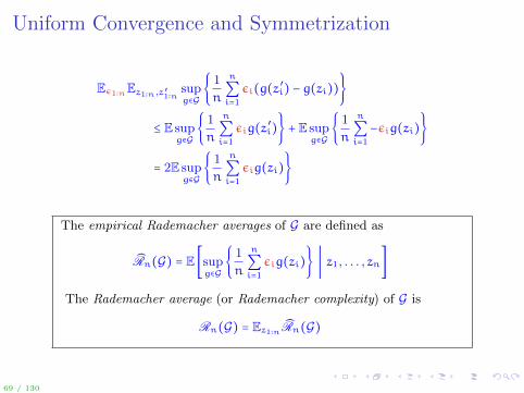
Uniform Convergence and Symmetrization

Eε1∶nEz1∶n,z ′1∶n

supg∈G

{ 1

n

n

∑i=1

εi(g(z ′i) − g(zi))}

≤ E supg∈G

{ 1

n

n

∑i=1

εig(z ′i)} + E supg∈G

{ 1

n

n

∑i=1

−εig(zi)}

= 2E supg∈G

{ 1

n

n

∑i=1

εig(zi)}

The empirical Rademacher averages of G are defined as

Rn(G) = E [supg∈G

{ 1

n

n

∑i=1

εig(zi)} ∣ z1, . . . , zn]

The Rademacher average (or Rademacher complexity) of G is

Rn(G) = Ez1∶nRn(G)

69 / 130

Classification: Loss Function Disappears

Let us focus on binary classification with indicator loss and let F be a classof {0, 1}-valued functions. We have

`(f(x),y) = I{f(x)≠y} = (1 − 2y)f(x) + y

and thus

Rn(G) = E [supf∈F

{ 1

n

n

∑i=1

εi(f(xi)(1 − 2yi) + yi)} ∣ (x1,y1) . . . , (xn,yn)]

= E [supf∈F

{ 1

n

n

∑i=1

εif(xi)} ∣ x1, . . . ,xn] = Rn(F)

because, given y1, . . . ,yn, the distribution of εi(1 − 2yi) is the same as εi.

70 / 130

Vapnik-Chervonenkis Theory for Classification

We are now left examining

E [supf∈F

{ 1

n

n

∑i=1

εif(xi)} ∣ x1, . . . ,xn]

Given x1, . . . ,xn, define the projection of F onto sample:

F ∣x1∶n = {(f(x1), . . . , f(xn)) ∈ {0, 1}n ∶ f ∈ F} ⊆ {0, 1}n

Clearly, this is a finite set and

Rn(F) = Eε1∶n maxv∈F ∣x1∶n

1

n

n

∑i=1

εivi ≤√

2 log card(F ∣x1∶n)n

This is because a maximum of N (sub)Gaussian random variables ∼√

logN.

The bound is nontrivial as long as log card(F ∣x1∶n) = o(n).

71 / 130


The growth function is defined as

ΠF(n) = max{card(F ∣x1,...,xn) ∶ x1, . . . ,xn ∈ X}

The growth function measures expressiveness of F . In particular, if F canproduce all possible signs (that is, ΠF(n) = 2n), the bound becomes useless.

We say that F shatters some set x1, . . . ,xn if F ∣xn = {0, 1}n.

The Vapnik-Chervonenkis (VC) dimension of the class F is defined as

vc(F) = max{d ∶ ΠF(t) = 2t}

Vapnik-Chervonenkis-Sauer-Shelah Lemma: If d = vc(F) <∞, then

ΠF(n) ≤d

∑i=0

(nd) ≤ (en

d)d

72 / 130


Conclusion: for any F with vc(F) <∞, the ERM algorithm satisfies

E{L(fn) − inff∈F

L(f)} ≤ 2

√2d log(en/d)

n

While we proved the result in expectation, the same type of bound holdswith high probability.

VC dimension is a combinatorial dimension of a binary-valued functionclass. Its finiteness is necessary and sufficient for learnability if we place noassumptions on the distribution P.

Remark: the bound is similar to that obtained through compression. Infact, the exact relationship between compression and VC dimension is stillan open question.

73 / 130


Examples of VC classes:

▸ Half-spaces F = {I{⟨w,x⟩+b≥0} ∶ w ∈ Rd, ∥w∥ = 1,b ∈ R} has vc(F) = d + 1

▸ For a vector space H of dimension d, VC dimension ofF = {I{h(x)≥0} ∶ h ∈H} is at most d

▸ The set of Euclidean balls F = {I{∑di=1 ∥xi−ai∥2≤b}∶ a ∈ Rd,b ∈ R} has

VC dimension at most d + 2.

▸ Functions that can be computed using a finite number of arithmeticoperations (see (Goldberg and Jerrum, 1995))

However: F = {fα(x) = I{sin(αx)≥0} ∶ α ∈ R} has infinite VC dimension, so itis not correct to think of VC dimension as the number of parameters!

Unfortunately, the VC theory is unable to explain the good performance ofneural networks and Support Vector Machines! This prompted thedevelopment of a margin-based theory.

74 / 130

Outline

Introduction



75 / 130

Classification with Real-Valued Functions

Many methods useI(F) = {I{f≥0} ∶ f ∈ F}

for classification. The VC dimension can be very large, yet in practice themethods work well.

Example: f(x) = fw(x) = ⟨w,ψ(x)⟩ where ψ is a mapping to a high-dimensional feature space (see Kernel Methods). The VC dimension of theset is typically huge (equal to the dimensionality of ψ(x)) or infinite, yetthe methods perform well!

Is there an explanation beyond VC theory?

76 / 130

Margins

Hard margin:∃f ∈ F ∶ ∀i, yif(xi) ≥ γ

f(x)

More generally, we hope to have

∃f ∈ F ∶ card({i ∶ yif(xi) < γ})n

is small

77 / 130

Surrogate LossDefine

φ(s) =⎧⎪⎪⎪⎪⎨⎪⎪⎪⎪⎩

1 if s ≤ 0

1 − s/γ if 0 < s < γ0 if s ≥ γ

Then: I{y≠sign(f(x))} = I{yf(x)≤0} ≤ φ(yf(x)) ≤ ψ(yf(x)) = I{yf(x)≤γ}

The function φ is an example of a surrogate loss function.

�(yf(x))

�

(yf(x))I{yf(x)60}

yf(x)

Let

Lφ(f) = Eφ(yf(x)) and Lφ(f) =1

n

n

∑i=1

φ(yif(xi))

ThenL(f) ≤ Lφ(f), Lφ(f) ≤ Lψ(f)

78 / 130

Surrogate Loss

Now consider uniform deviations for the surrogate loss:

E supf∈F

{Lφ(f) − Lφ(f)}

We had shown that this quantity is at most 2Rn(φ(F)) for

φ(F) = {g(z) = φ(yf(x)) ∶ f ∈ F}

A useful property of Rademacher averages:

Rn(φ(F)) ≤ LRn(F) if φ is L-Lipschitz.

Observe that in our example φ is 1/γ-Lipschitz. Hence,

E supf∈F

{Lφ(f) − Lφ(f)} ≤2

γRn(F)

79 / 130

Margin BoundSame result in high probability: with probability at least 1 − δ,

supf∈F

{Lφ(f) − Lφ(f)} ≤2

γRn(F) +

√log(1/δ)

2n

With probability at least 1 − δ, for all f ∈ F

L(f) ≤ Lψ(f) +2

γRn(F) +

√log(1/δ)

2n

If fn is minimizing margin loss

fn = arg minf∈F

1

n

n

∑i=1

φ(yif(xi))

then with probability at least 1 − δ

L(fn) ≤ inff∈F

Lψ(f) +4

γRn(F) + 2

√log(1/δ)

2n

Note: φ assumes knowledge of γ, but this assumption can be removed.

80 / 130

Outline

Introduction



81 / 130

Useful Properties

1. If F ⊆ G, then Rn(F) ≤ Rn(G)2. Rn(F) = Rn(conv(F))3. For any c ∈ R, Rn(cF) = ∣c∣Rn(F)4. If φ ∶ R↦ R is L-Lipschitz (that is, φ(a) −φ(b) ≤ L∣a − b∣ for alla,b ∈ R), then

Rn(φ ○F) ≤ LRn(F)

82 / 130

Rademacher Complexity of Kernel Classes

▸ Feature map φ ∶ X ↦ `2 and p.d. kernel K(x1,x2) = ⟨φ(x1),φ(x2)⟩▸ The set FB = {f(x) = ⟨w,φ(x)⟩ ∶ ∥w∥ ≤ B} is a ball in H▸ Reproducing property f(x) = ⟨f,K(x, ⋅)⟩

An easy calculation shows that empirical Rademacher averages are upperbounded as

Rn(FB) = E supf∈F1

1

n

n

∑i=1

εif(xi) = E supf∈FB

1

n

n

∑i=1

εi ⟨f,K(xi, ⋅)⟩

= E supf∈FB

⟨f, 1

n

n

∑i=1

εiK(xi, ⋅)⟩ = B ⋅ E∥ 1

n

n

∑i=1

εiK(xi, ⋅)∥

= BnE⎛⎝n

∑i,j=1

εiεj ⟨K(xi, ⋅),K(xj, ⋅)⟩⎞⎠

−1/2

≤ Bn

(n

∑i=1

K(xi,xi))−1/2

A data-independent bound of O(Bκ/√n) can be obtained if

supx∈X K(x,x) ≤ κ2. Then κ and B are the effective “dimensions”.

83 / 130

Other Examples

Using properties of Rademacher averages, we may establish guarantees forlearning with neural networks, decision trees, and so on.

Powerful technique, typically requires only a few lines of algebra.

Occasionally, covering numbers and scale-sensitive dimensions can be easierto deal with.

84 / 130

Outline

Introduction



85 / 130

Real-Valued Functions: Covering NumbersConsider

▸ a class F of [−1, 1]-valued functions

▸ let Y = [−1, 1], `(f(x),y) = ∣f(x) − y∣

We haveE supf∈F

L(f) − L(f) ≤ 2Ex1∶nRn(F)

For real-valued functions the cardinality of F ∣x1∶n is infinite. However,similar functions f and f ′ with

(f(x1), . . . , f(xn)) ≈ (f ′(x1), . . . , f ′(xn))

should be treated as the same.

↵

86 / 130

Real-Valued Functions: Covering Numbers

Given α > 0, suppose we can find V ⊂ [−1, 1]n of finite cardinality such that

∀f,∃vf ∈ V, s.t.1

n

n

∑i=1

∣f(xi) − vfi ∣ ≤ α

Then

Rn(F) = Eε1∶n supf∈F

1

n

n

∑i=1

εif(xi)

= Eε1∶n supf∈F

1

n

n

∑i=1

εi(f(xi) − vfi) + Eε1∶n supf∈F

1

n

n

∑i=1

εivfi

≤ α + Eε1∶n maxv∈V

1

n

n

∑i=1

εivi

Now we are back to the set of finite cardinality:

Rn(F) ≤ α +√

2 log card(V)n

87 / 130


Such a set V is called an α-cover (or α-net). More precisely, a set V is anα-cover with respect to `p norm if

∀f,∃vf ∈ V, s.t.1

n

n

∑i=1

∣f(xi) − vfi ∣p ≤ αp

The size of the smallest α-cover is denoted by Np(F ∣x1∶n ,α).

x1 x2 xT

Above : Two sets of levels provide an α-cover for the four functions. Onlythe values of functions on x1, . . . ,xT are relevant.

88 / 130


We have proved that for any x1, . . . ,xn,

Rn(F) ≤ infα≥0

{α + 1√n

√2 log card(N1(F ∣x1∶n ,α))}

A better bound (called Dudley entropy integral):

Rn(F) ≤ infα≥0

{4α + 12√n∫

1

α

√2 log card(N2(F ∣x1∶n , δ))dδ}

89 / 130

Example: Nondecreasing functions.

Consider the set F of nondecreasing functions R↦ [−1, 1].

While F is a very large set, F ∣x1∶n is not that large:

N1(F ∣x1∶n ,α) ≤ N2(F ∣x1∶n ,α) ≤ n2/α.

The first bound on the previous slide yields

infα≥0

{α + 1√αn

√4 log(n)} = O(n−1/3)

while the second bound (the Dudley entropy integral)

infα≥0

{4α + 12√n∫

1

α

√4/δ log(n)dδ} = O(n−1/2)

where the O notation hides logarithmic factors.

90 / 130

Scale-Sensitive Dimensions

We say that F ⊆ RX α-shatters a set (x1, . . . ,xT ) if there exist(y1, . . . ,yT ) ∈ RT (called a witness to shattering) with the followingproperty:

∀(b1, . . . ,bT ) ∈ {0, 1}T , ∃f ∈ F s.t.

f(xt) > yt +α

2if bt = 1 and f(xt) < yt −

α

2if bt = 0

The fat-shattering dimension of F at scale α, denoted by fat(F ,α), is thesize of the largest α-shattered set.

Wait, another measure of complexity of F? How is it related to coveringnumbers?

Theorem (Mendelson & Vershynin): For F ⊆ [−1, 1]X and any 0 < α < 1,

N2(F ∣x1∶n ,α) ≤ ( 2

α)K⋅fat(F,cα)

where K, c are positive absolute constants.

91 / 130

Quick Summary

We are after uniform deviations in order to understand performance ofERM. Rademacher averages is a nice measure with useful properties. Theycan be further upper bounded by covering numbers through the Dudleyentropy integral. In turn, covering numbers can be controlled via thefat-shattering combinatorial dimension. Whew!

92 / 130

Outline

Introduction



93 / 130

Faster Rates

Are there situations when

EL(fn) − inff∈F

L(f)

approaches 0 faster than O(1/√n)?

Yes! We can beat the Central Limit Theorem!

How is this possible??

Recall that the CLT tells us about convergence of average to theexpectation for random variables with bounded second moment. What ifthis variance is small?

94 / 130

Faster Rates: Classification

Consider the problem of binary classification with the indicator loss and aclass F of {0, 1}-valued functions. For any f ∈ F ,

1

n

n

∑i=1

`(f(xi),yi)

is an average of n Bernoulli random variables with bias p = E`(f(x),y).Exact expression for the binomial tails:

P (L(f) − L(f) > ε) =⌊n(p−ε)⌋∑i=0

(ni)pi(1 − p)n−i

Further upper bounds:

exp{− nε2

2p(1 − p) + 2ε/3} Bernstein

exp{−2nε2} Hoeffding

95 / 130


Inverting

exp{− nε2

2p(1 − p) + 2ε/3} ≤ exp{− nε2

2p + 2ε/3} =∶ δ

yields that for any f ∈ F , with probability at least 1 − δ

L(f) ≤ L(f) +√

2L(f) log(1/δ)n

+ 2 log(1/δ)3n

For non-negative numbers A,B,C

A ≤ B +C√A implies A ≤ B +C2 +

√BC

Therefore for any f ∈ F , with probability at least 1 − δ,

L(f) ≤ L(f) +√

2L(f) log(1/δ)n

+ 4 log(1/δ)n

96 / 130


By the Union Bound, for F with finite N = card(F), with probability atleast 1 − δ,

∀f ∈ F ∶ L(f) ≤ L(f) +√

2L(f) log(N/δ)n

+ 4 log(N/δ)n

For an empirical minimizer fn, with probability at least 1 − δ, a zeroempirical loss L(fn) = 0 implies

L(fn) ≤4 log(N/δ)

n

This happens, for instance, in the so-called noiseless case: L(fF) = 0.Indeed, then L(fF) = 0 and thus L(fn) = 0.

97 / 130

Summary: Minimax Viewpoint

Value of a game where we choose an algorithm, Nature chooses adistribution P ∈ P, and our payoff is the expected loss of our algorithmrelative to the best in F :

Viid(F ,P,n) = inffn

supP∈P

{L(fn) − inff∈F

L(f)}

If we make no assumption on the distribution P, then P is the set of alldistributions. Many of the results we obtained in this lecture are for thisdistribution-free case. However, one may view margin-based results and theabove fast rates for the noiseless case as studying Viid(F ,P,n) when P is“nicer”.

98 / 130

Outline

Introduction



99 / 130

Model Selection

For a given class F , we have proved statements of the type

P (supf∈F

{L(f) − L(f)} ≥ φ(δ,n,F)) < δ

Now, take a countable nested sieve of models

F1 ⊆ F2 ⊆ ...

such that H = ∪∞i=1Fi is a very large set that will surely capture the Bayesfunction.

For a function f ∈H, let k(f) be the smallest index of Fk that contains f.Let us write φn(δ, i) for φ(δ,n,Fi).

Let us put a distribution w(i) on the models, with ∑∞i=1w(i) = 1. Then for

every i,

P (supf∈Fi

{L(f) − L(f)} ≥ φn(δw(i), i)) < δ ⋅w(i)

simply by replacing δ with δw(i).

100 / 130

Now, taking a union bound:

P (supf∈H

{L(f) − L(f)} ≥ φn(δw(k(f)),k(f))) <∑i

δw(i) ≤ δ

Consider the penalized method

fn = arg minf∈H

{L(f) +φn(δw(k(f)),k(f))}

= arg mini,f∈Fi

{L(f) +φn(δw(i), i)}

This balances fit to data and the complexity of the model. Of course, thisis exactly a regularized ERM form analyzed earlier.

F1

Fk⇤

f⇤. . .. . .

Let k∗ = k(f∗) be the (smallest) model Fi that contains the optimalfunction.

101 / 130

Exactly as on the slide “Countable Class: Weighted Union Bound”,

L(fn) − L(f∗) ≤ {L(fn) − L(fn) − penn(fn)}+ {L(fn) + penn(fn) − L(fF) − penn(fF)}+ {L(fF) − L(fF)} + penn(fF)≤ L(f∗) − L(f∗) + penn(f

∗)= L(f∗) − L(f∗) +φn(δw(k∗),k∗)

The first part of this bound is OP(1/√n) by the CLT, just as before.

If the dependence of φ on 1/δ is logarithmic, then taking w(i) = 2−i simplyimplies an additional additive i∗, a penalty for not knowing the model inadvance.

Conclusion: given uniform deviation bounds for a single class F , asdeveloped earlier, we can perform model selection by penalizing modelcomplexity!

102 / 130

Outline

Introduction



103 / 130

Outline

Introduction



104 / 130

Looking back: Statistical Learning

▸ future looks like the past

▸ modeled as i.i.d. data

▸ evaluated on a random sample from the same distribution

▸ developed various measures of complexity of F

105 / 130

Example #1: Bit Prediction

Predict a binary sequence y1,y2, . . . ∈ {0, 1}, which is revealed one by one.At step t, make a prediction zt of the t-th bit, then yt is revealed.

Let ct = I{zt=yt}. Goal: make cn = 1n ∑

nt=1 ct large.

Suppose we are told that the sequence presented is Bernoulli with anunknown bias p. How should we choose predictions?

106 / 130

Example #1: Bit Prediction

Of course, we should do majority vote over the past outcomes

zt = I{yt−1≥1/2}

where yt−1 = 1t−1 ∑

t−1s=1 ys. This algorithm guarantees ct →max{p, 1−p} and

lim inft→∞

(ct −max{zt, 1 − zt}) ≥ 0 almost surely (∗)

Claim: there is an algorithm that ensures (∗) for an arbitrary sequence.Any idea how to do it?

Another way to formulate (∗): number of mistakes should be not muchmore than made by the best of the two “experts”, one predicting “1” all thetime, the other constantly predicting “0”.

Note the difference: estimating a hypothesized model vscompeting against a reference set. We had seen this distinction inthe previous lecture.

107 / 130

Example #2: Email Spam Detection

We are tasked with developing a spam detection program thatneeds to be adaptive to malicious attacks.

▸ x1, . . . ,xn are email messages, revealed one-by-one

▸ upon observing the message xt, the learner (spam detector) needs todecide whether it is spam or not spam (yt ∈ {0, 1})

▸ the actual label yt ∈ {0, 1} is revealed (e.g. by the user)

Do it seem plausible that (x1,y1), . . . , (xn,yn) are i.i.d. from somedistribution P?

Probably not... In fact, the sequence might even be adversarially chosen. Infact, spammers adapt and try to improve their strategies.

108 / 130

Outline

Introduction



109 / 130

Online Learning (Supervised)

▸ No assumption that there is a single distribution P

▸ Data not given all at once, but rather in the online fashion

▸ As before, X is the space of inputs, Y the space of outputs

▸ Loss function `(y1,y2)

Online protocol (supervised learning):

For t = 1, . . . ,nObserve xt, predict yt, observe yt

Goal: keep regret small:

Regn =1

n

n

∑t=1

`(yt,yt) − inff∈F

1

n

n

∑t=1

`(f(xt),yt)

A bound on Regn should hold for any sequence (x1,y1), . . . , (xn,yn)!

110 / 130

Pros/Cons of Online Learning

The good:

▸ An upper bound on regret implies good performance relative to the setF no matter how adversarial the sequence is.

▸ Online methods are typically computationally attractive as theyprocess one data point at a time. Used when data sets are huge.

▸ Interesting research connections to Game Theory, Information Theory,Statistics, Computer Science.

The bad:

▸ A regret bound implies good performance only if one of the elementsof F has good performance (just as in Statistical Learning). However,for non-iid sequences a single f ∈ F might not be good at all! Toalleviate this problem, the comparator set F can be made into a set ofmore complex strategies.

▸ There might be some (non-i.i.d.) structure of sequences that we arenot exploiting (this is an interesting area of research!)

111 / 130

Setting Up the Minimax Value

First, it turns out that yt has to be a randomized prediction: we need todecide on a distribution qt ∈ ∆(Y) and then draw yt from qt.

The minimax best that both the learner and the adversary (or, Nature) cando is

V(F ,n) = ⟪ supxt∈X

infqt∈∆

supyt∈Y

Eyt∼qt

⟫n

t=1

{ 1

n

n

∑t=1

`(yt,yt) − inff∈F

1

n

n

∑t=1

`(f(xt),yt)}

This is an awkward and long expression, so no need to be worried. All youneed to know right now is:

▸ An upper bound on V(F ,n) guarantees existence of a strategy(learning algorithm) that will suffer at most that much regret.

▸ A lower bound on V(F ,n) means the adversary can inflict at leastthat much damage, no matter what the learning algorithm does.

It is interesting to study V(F ,n)! It turns out, many of the tools we usedin Statistical Learning can be extended to study Online Learning!

112 / 130

Sequential Rademacher Complexity

A (complete binary) X -valued tree x of depth n is a collection of functionsx1, . . . ,xn such that xi ∶ {±1}i−1 ↦ X and x1 is a constant function.

A sequence ε = (ε1, . . . ,εn) defines a path in x:

x1, x2(ε1), x3(ε1,ε2), . . . , xn(ε1, . . . ,εn−1)

Define sequential Rademacher complexity as

Rseqn (F ,n) = sup

xEε1∶n sup

f∈F{ 1

n

n

∑t=1

εtf(xt(ε1∶t−1))}

where the supremum is over all X -valued trees of depth n.

TheoremLet Y = {0, 1} and F is a class of binary-valued functions. Let ` be theindicator loss. Then

V(F ,n) ≤ 2Rseqn (F ,n)

113 / 130

Finite Class

Suppose F is finite, N = card(F). Then for any tree x,

Eε1∶n supf∈F

{ 1

n

n

∑t=1

εtf(xt(ε1∶t−1))} ≤√

2 logN

n

because, again, this is a maximum of N (sub)Gaussian Random variables!

Hence,

V(F ,n) ≤ 2

√2 logN

n

This bound is basically the same as that for Statistical Learning with afinite number of functions!

Therefore, there must exist an algorithm for predicting yt given xt such

that regret scales as O(√

logNn

). What is it?

114 / 130

Exponential Weights, or the Experts Algorithm

We think of each element {f1, . . . , fN} = F as an expert who gives aprediction fi(xt) given side information xt. We keep distribution wt overexperts, according to their performance.

Let w1 = (1/N, . . . , 1/N), η =√

(8 logN)/T .

To predict at round t, observe xt, pick it ∼ wt and set yt = fit(xt).

Updatewt+1(i)∝ wt(i) exp{−ηI{fi(xt)≠yt}}

Claim: for any sequence (x1,y1), . . . , (xn,yn), with probability at least 1− δ

1

n

n

∑t=1

I{yt≠yt} − inff∈F

1

n

n

∑t=1

I{f(xt)≠yt} ≤√

logN

2n+√

log(1/δ)2n

115 / 130

Useful Properties of Sequential Rademacher Complexity

Sequential Rademacher complexity enjoys the same nice properties as its iidcousin, except for the Lipschitz contraction (4). At the moment we canonly prove

Rseqn (φ ○F) ≤ LRseq

n (F) ×O(log3/2n)

It is an open question whether this logarithmic factor can be removed...

116 / 130

Theory for Online Learning

There is now a theory with combinatorial parameters, covering numbers,and even a recipe for developing online algorithms!

Many of the relevant concepts (e.g. sequential Rademacher complexity) aregeneralizations of the i.i.d. analogues to the case of dependent data.

Coupled with the online-to-batch conversion we introduce in a few slides,there is now an interesting possibility of developing new computationallyattractive algorithms for statistical learning. One such example will bepresented.

117 / 130

Theory for Online Learning

Statistical Learning Online Learning

i.i.d. data arbitrary sequences

tuples of data binary trees

Rademacher averages sequential Rademacher complexity

covering / packing numbers tree cover

Dudley entropy integral analogous result with tree cover

VC dimension Littlestone’s dimension

Scale-sensitive dimension analogue for trees

Vapnik-Chervonenkis-Sauer-ShelahLemma analogous combinatorial result for trees

ERM and regularized ERM many interesting algorithms

118 / 130

Outline

Introduction



119 / 130

Online Convex and Linear Optimization

For many problems, `(f, (x,y)) is convex in f and F is a convex set. Let ussimply write `(f, z), where the move z need not be of the form (x,y).

▷ e.g. square loss `(f, (x,y)) = (⟨f,x⟩ − y)2 for linear regression.

▷ e.g. hinge loss `(f, (x,y)) = max{0, 1 − y ⟨f,x⟩}, a surrogate loss forclassification.

We may then use optimization algorithms for updating our hypothesis afterseeing each additional data point.

120 / 130

Online Convex and Linear Optimization

Online protocol (Online Convex Optimization):

For t = 1, . . . ,nPredict ft ∈ F , observe zt

Goal: keep regret small:

Regn =1

n

n

∑t=1

`(ft, zt) − inff∈F

1

n

n

∑t=1

`(f, zt)

Online Linear Optimization is a particular case when `(f, z) = ⟨f, z⟩.

121 / 130

Gradient Descent

At time t = 1, . . . ,n, predict ft ∈ F , observe zt, update

f′t+1 = ft − η∇`(ft, zt)

and project f ′t+1 to the set F , yielding ft+1.

▸ η is a learning rate (step size)

▸ gradient is with respect to the first coordinate

This simple algorithm guarantees that for any f ∈ F

1

n

n

∑t=1

`(ft, zt) −1

n

n

∑t=1

`(f, zt) ≤1

n

n

∑t=1

⟨ft,∇`(ft, zt)⟩ −1

n

n

∑t=1

⟨f,∇`(ft, zt)⟩

≤ O(n−1/2)

as long as ∥∇`(ft, zt)∥ ≤ c for some constant c, for all t, and F has abounded diameter.

122 / 130

Gradient Descent for Strongly Convex Functions

Assume that for any z, `(⋅, z) is strongly convex in the first argument. Thatis, `(f, z) − 1

2∥f∥2 is a convex function.

The same gradient descent algorithm with a different step size η guaranteesthat for any f∗ ∈ F

1

n

n

∑t=1

`(ft, zt) −1

n

n

∑t=1

`(f, zt) ≤ O( log(n)n

) ,

a faster rate.

123 / 130

Outline

Introduction



124 / 130

How to use regret bounds for i.i.d. data

Suppose we have a regret bound

1

n

n

∑t=1

`(ft, zt) − inff∈F

1

n

n

∑t=1

`(f, zt) ≤ Rn

that holds for all sequences z1, . . . , zn, for some Rn → 0.

Assume z1, . . . , zn are i.i.d. with distribution P. Run the regretminimization algorithm on these data and let f = 1

n ∑nt=1 ft. Then

Ez,z1,...,zn`(f, z) ≤ E{ 1

n

n

∑t=1

`(ft, z)} = E{ 1

n

n

∑t=1

`(ft, zt)}

where the last step holds because ft only depends on z1, . . . , zt−1. Also,

E{inff∈F

1

n

n

∑t=1

`(f, zt)} ≤ inff∈F

E{ 1

n

n

∑t=1

`(f, zt)} = Ez`(fF , z)

Combining,EL(f) − inf

f∈FL(f) ≤ Rn

125 / 130

How to use regret bounds for i.i.d. data

This gives an alternative way of proving bounds on

EL(fn) − inff∈F

L(f)

by using fn = f, the average of the trajectory of an online learningalgorithm.

Next, we present an interesting application of this idea.

126 / 130

Pegasos

Support Vector Machine is a fancy name for the algorithm

fn = arg minf∈Rd

1

m

m

∑i=1

max{0, 1 − yi ⟨f,xi⟩} +λ

2∥f∥2

in the linear case.

The objective can be “kernelized” for representing linear separators inhigher-dimensional feature space. The hinge loss is convex in f.

Write

`(f, z) = max{0, 1 − y ⟨f,x⟩} + λ2∥f∥2

for z = (x,y). Then the objective of SVM can be written as

minf

E`(f, z)

The expectation is with respect to the empirical distribution 1m ∑

mi=1 δ(xi,yi).

Then an i.i.d. sample z1, . . . , zn from the empirical distribution is simply adraw with replacement from the dataset {(x1,y1), . . . , (xm,ym)}.

127 / 130

Pegasos

A gradient descent ft+1 = ft − η∇`(ft, zt) with

∇`(ft, zt) = −ytxtI{yt⟨ft,xt⟩<1} + λft

then gives a guarantee

E`(f, z) − inff∈F

E`(f, z) ≤ Rn

Since `(f, z) is λ-strongly convex, the rate Rn = O(log(n)/n).

Pegasos (Shalev-Shwartz et al, 2010)For t = 1, . . . ,nChoose a random example (xit ,yit) from the dataset. Set η = 1/(λt)If yit ⟨ft,xit⟩ < 1, update ft+1 = (1 − ηtλ)ft + ηtxityitelse, update ft+1 = (1 − ηtλ)ft

The algorithm and analysis are due to (S. Shalev-Shwartz, Singer, Srebro, Cotter, 2010)

128 / 130

Pegasos

We conclude that f = 1n ∑

nt=1 ft computed using the gradient descent

algorithm is an O(n−1)-approximate minimizer of the SVM objective aftern steps.

This gives an O(d/(λε)) time to converge to an ε-minimizer. Very fastSVM solver, attractive for large datasets!

129 / 130

Summary

Key points for both statistical and online learning:

▸ obtained performance guarantees with minimal assumptions

▸ prior knowledge is captured by the comparator term

▸ understanding the inherent complexity of the comparator set

▸ key techniques: empirical processes for iid and non-iid data

▸ interesting relationships between statistical and online learning

▸ computation and statistics – a basis of machine learning

130 / 130

statistical learning theory - statistics...

Documents