statistical methods for nlp - cs.columbia.edu
TRANSCRIPT

1
Statistical Methods for NLP
Part I Markov Random FieldsPart II Equations to Implementation
Sameer Maskey
Week 14, April 20, 2010

2
Announcement
� Next class : Project presentation
� 10 mins total time, strictly timed
� 2 mins for questions
� Please come to my office hours to download the presentation to my laptop
� Or please come 15 mins early to the class
3
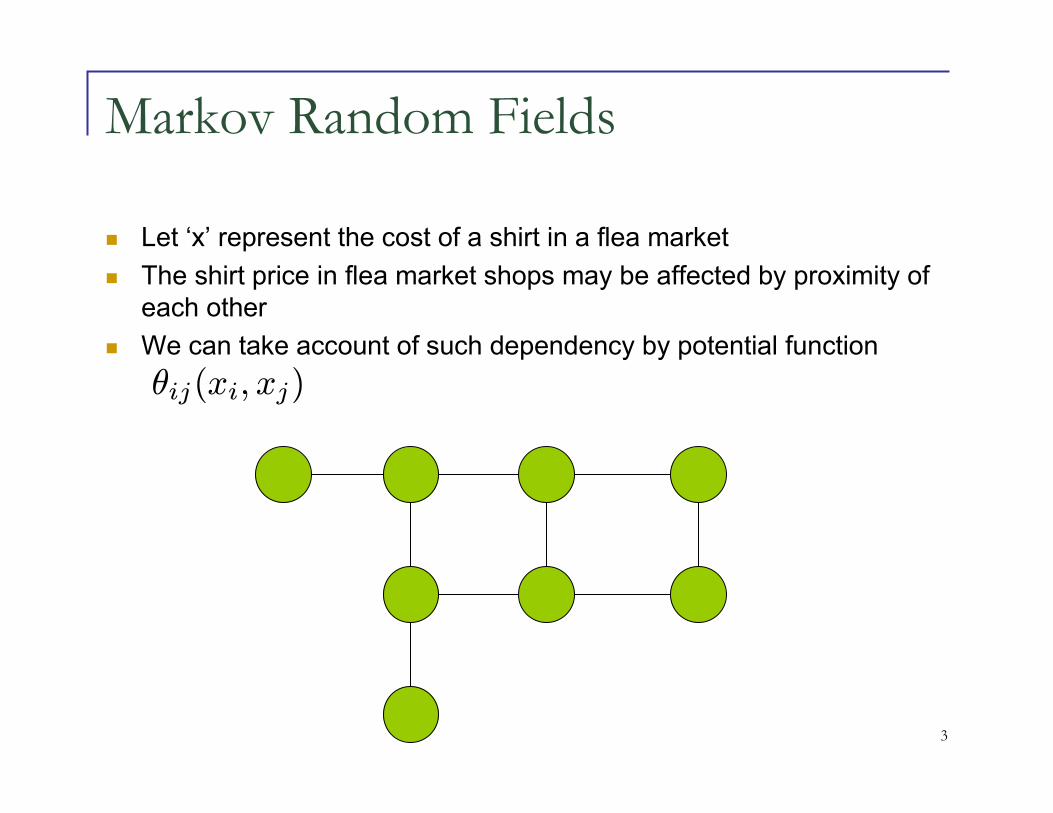
Markov Random Fields
� Let ‘x’ represent the cost of a shirt in a flea market
� The shirt price in flea market shops may be affected by proximity of each other
� We can take account of such dependency by potential function
θij(xi, xj)
4
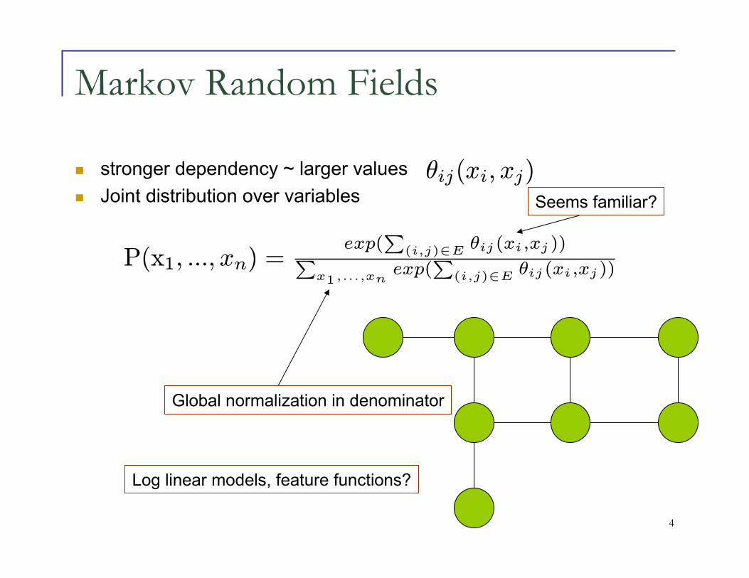
Markov Random Fields
� stronger dependency ~ larger values
� Joint distribution over variables
θij(xi, xj)
P(x1, ..., xn) =exp(
∑(i,j)∈E θij(xi,xj))∑
x1,...,xnexp(
∑(i,j)∈E θij(xi,xj))
Global normalization in denominator
Seems familiar?
Log linear models, feature functions?

5
Markov Random Fields (cont’d)
� Rewriting in terms of factors
P(x1, ..., xn) =1Z(θ)exp(
∑(i,j)∈E θij(xi, xj))
= 1Z(θ)
∏(i,j)∈E exp(θij(xi, xj))
= 1Z(θ)
∏(i,j)∈E ψij(xi, xj)
Potential Functions
Positive functions over groups of variables

6
Potential Functions
� Potential is just a table (all node combinations represented as entries)
� Marginalizing the potential entails collapsing into one dimension
Marginalize over B Marginalize over A
7
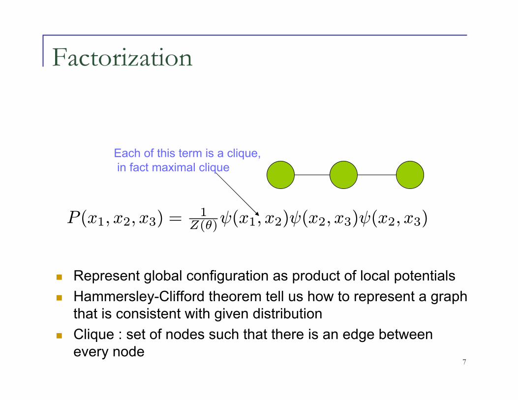
Factorization
P (x1, x2, x3) =1Z(θ)ψ(x1, x2)ψ(x2, x3)ψ(x2, x3)
Each of this term is a clique,in fact maximal clique
� Represent global configuration as product of local potentials
� Hammersley-Clifford theorem tell us how to represent a graph that is consistent with given distribution
� Clique : set of nodes such that there is an edge between every node
8
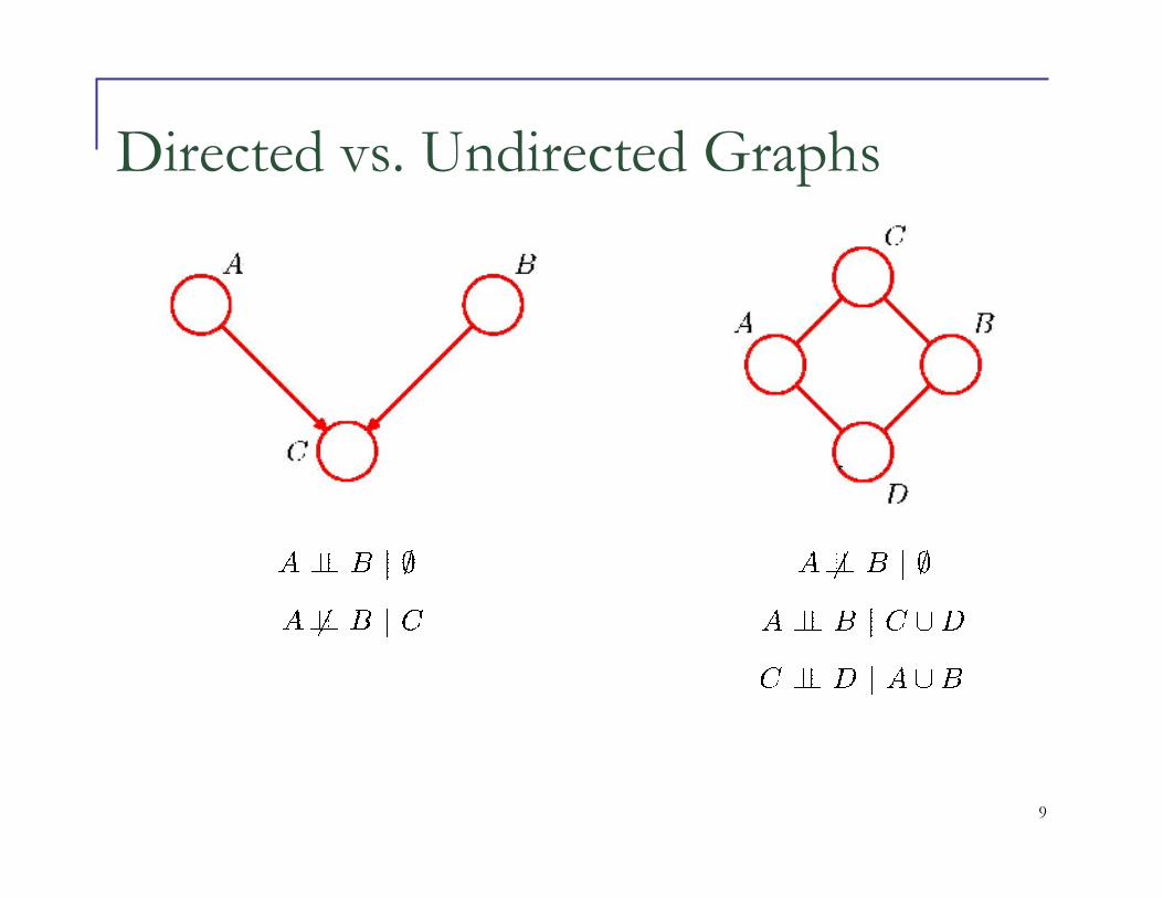
Graph Separation
� We liked Bayesian Network because it allowed to represent conditional independence well
� Conditional independence governed by D-separation criterion in Bayes Net
� Simple representation of independence properties in Markov Random Field
� Check graph reachability
9
Directed vs. Undirected Graphs

10
Converting Directed to Undirected Graphs
� Additional links
11
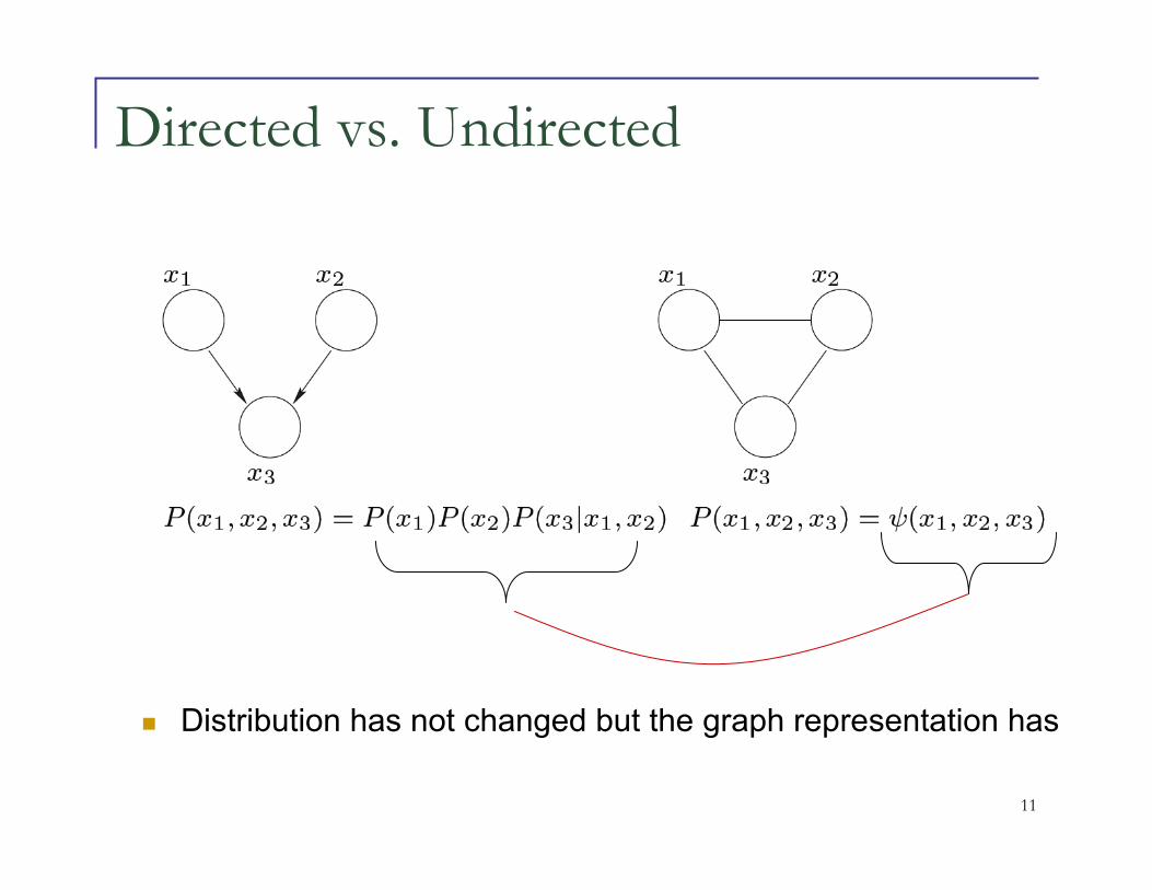
Directed vs. Undirected
� Distribution has not changed but the graph representation has
12
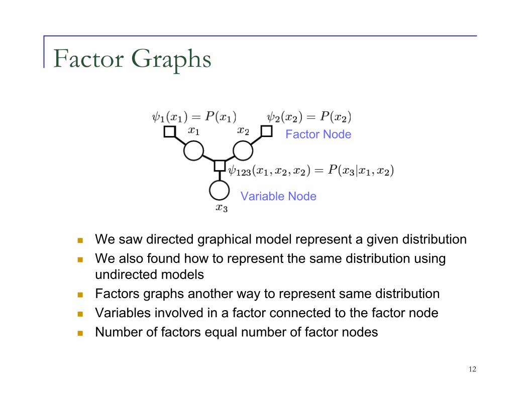
Factor Graphs
� We saw directed graphical model represent a given distribution
� We also found how to represent the same distribution using undirected models
� Factors graphs another way to represent same distribution
� Variables involved in a factor connected to the factor node
� Number of factors equal number of factor nodes
Variable Node
Factor Node

13
Graph Representation
� We saw that we can represent distributions in three different types of graphs
� Directed Acyclic Graphs
� Undirected Graphs
� Factor Graphs
� Depending on a problem one type of graph may be favored against another

14
Graphical Models in NLP
� Markov Random Field for term dependencies [Metzler W and Croft D, 05]
� Conditional Random fields for shallow parsing [Sha F. and Pereira F, 03]
� Bayesian Network for speech summarization [Maskey S. and Hirschberg J., 03]
� Dependency parsing with belief propagation [Smith D and Eisner J, 08]
15
Inference in Graphical Model
� Weights in Network make local assertions on how two nodes are related
� Inference algorithm takes these local assertions into global assertions between nodes[Jordan, M, 02]
� Many inference algorithms
� Popular inference algorithm : Junction Tree algorithm
16
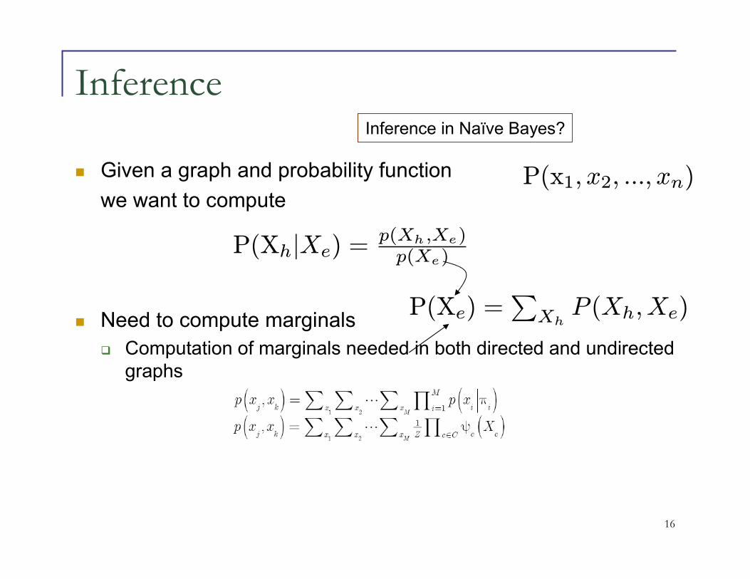
Inference
� Given a graph and probability function
we want to compute
� Need to compute marginals
� Computation of marginals needed in both directed and undirected graphs
P(x1, x2, ..., xn)
P(Xh|Xe) =p(Xh,Xe)p(Xe)
Inference in Naïve Bayes?
P(Xe) =∑XhP (Xh,Xe)
17
Inference : Exploit Graph Structure
� We can compute marginals by summing over all other variables
� Brute force, computationally expensive, not efficient
� Better algorithm?
� Pass messages in the graph
� Enforce consistency among messages
18
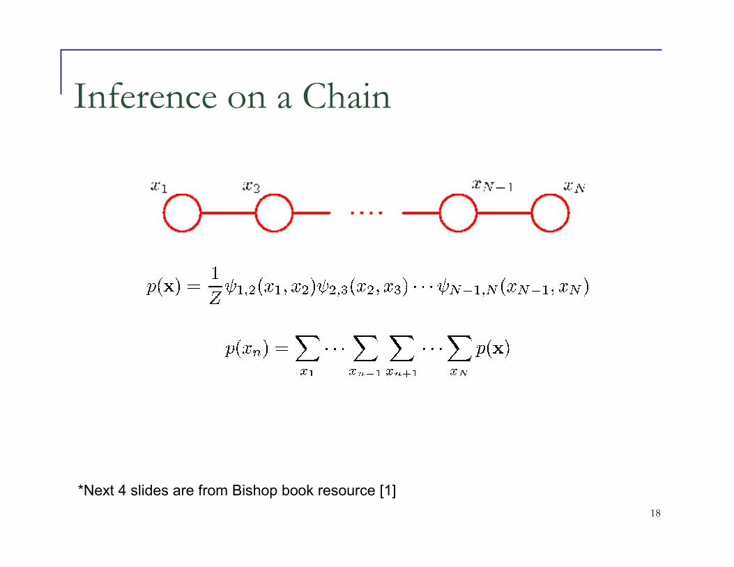
Inference on a Chain
*Next 4 slides are from Bishop book resource [1]

19
Inference on a Chain

20
Inference on a Chain
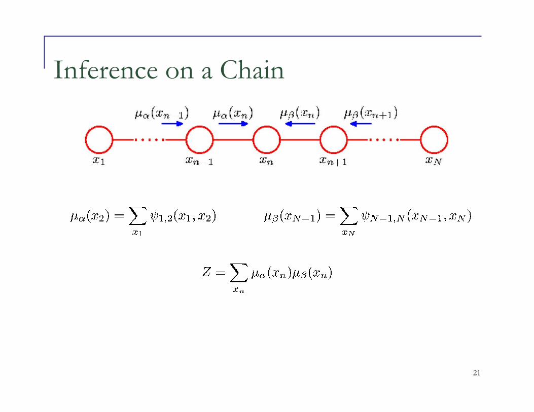
21
Inference on a Chain
22
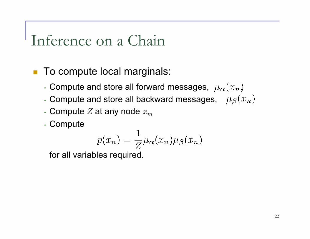
Inference on a Chain
� To compute local marginals:
• Compute and store all forward messages, .
• Compute and store all backward messages, .
• Compute Z at any node xm
• Compute
for all variables required.

23
MOD
Graphical Model for Dependency Parsing
He reckons the current account deficit will narrow to only 1.8 billion in September.
Raw sentence
Part-of-speech tagging
He reckons the current account deficit will narrow to only 1.8 billion in September.PRP VBZ DT JJ NN NN MD VB TO RB CD CD IN NNP .
POS-tagged sentence
Word dependency parsing
slide from Smith D and Eisner J, 08, [2]
Word dependency parsed sentence
He reckons the current account deficit will narrow to only 1.8 billion in September .
SUBJ
ROOT
S-COMP
SUBJ
SPEC
MODMOD
COMP
COMP
24
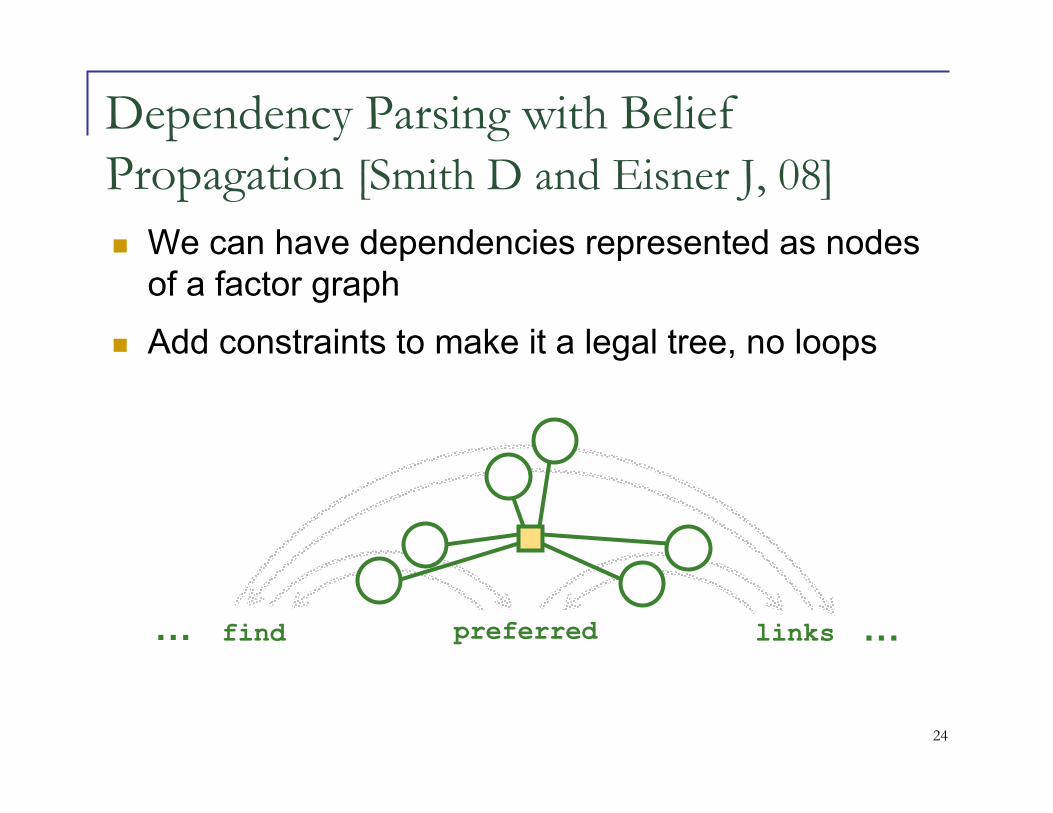
Dependency Parsing with Belief
Propagation [Smith D and Eisner J, 08]
find preferred links ……
� We can have dependencies represented as nodes of a factor graph
� Add constraints to make it a legal tree, no loops
25
Graphical Models Summary
� Represent distributions with graphs (directed, undirected, factor graphs)
� Inference on the graph can be done by message passing algorithms
� Gaining more attention in NLP community

26
Statistical Methods for NLP
Part II Equations to Implementation

27
Topics We Covered
NLP -- ML� Text Mining
� Text Categorization
� Information Extraction
� Topic and Document Clustering
� Machine Translation
� Language Modeling� Speech-to-Speech Translation
Linear Models of Regression
Linear Methods of ClassificationSupport Vector Machines
Hidden Markov ModelMaximum Entropy ModelsConditional Random Fields
K-meansExpectation Maximization Viterbi Search
Graphical Models

28
Scoring Unstructured Text
Patterns may exist in unstructured text
Some of these patternscould be exploited todiscover knowledge
All Amazon reviewers may notrate the product, may just
write reviews, we may have to infer the rating based on text review
Review of a camera in Amazon
29
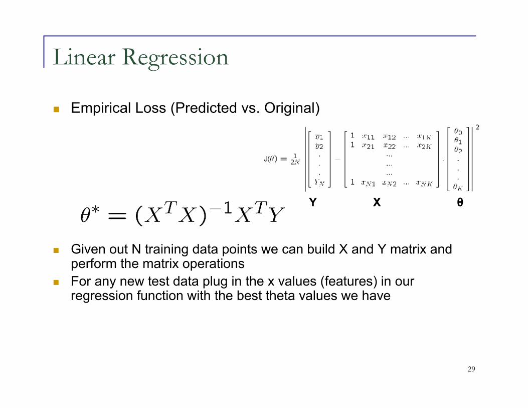
Linear Regression
� Empirical Loss (Predicted vs. Original)
Y X θ
� Given out N training data points we can build X and Y matrix andperform the matrix operations
� For any new test data plug in the x values (features) in our regression function with the best theta values we have
30
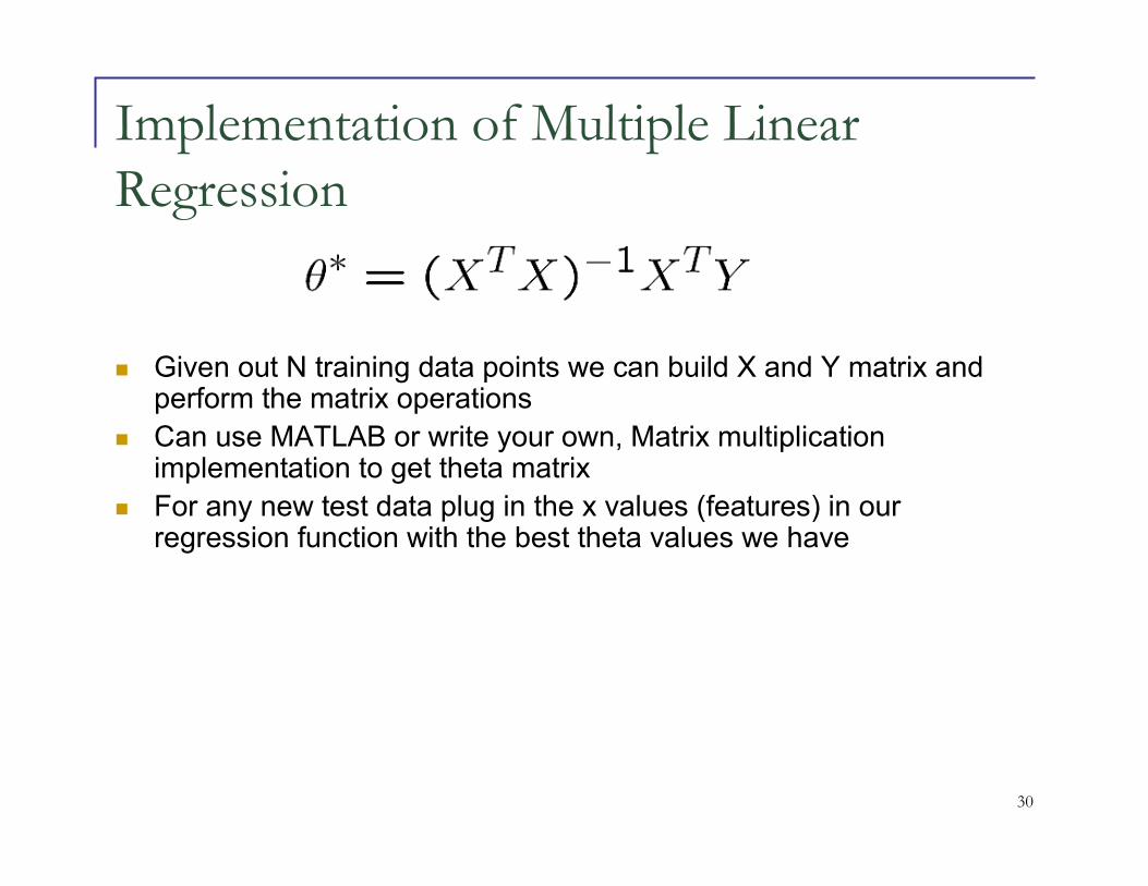
Implementation of Multiple Linear
Regression
� Given out N training data points we can build X and Y matrix andperform the matrix operations
� Can use MATLAB or write your own, Matrix multiplication implementation to get theta matrix
� For any new test data plug in the x values (features) in our regression function with the best theta values we have
31
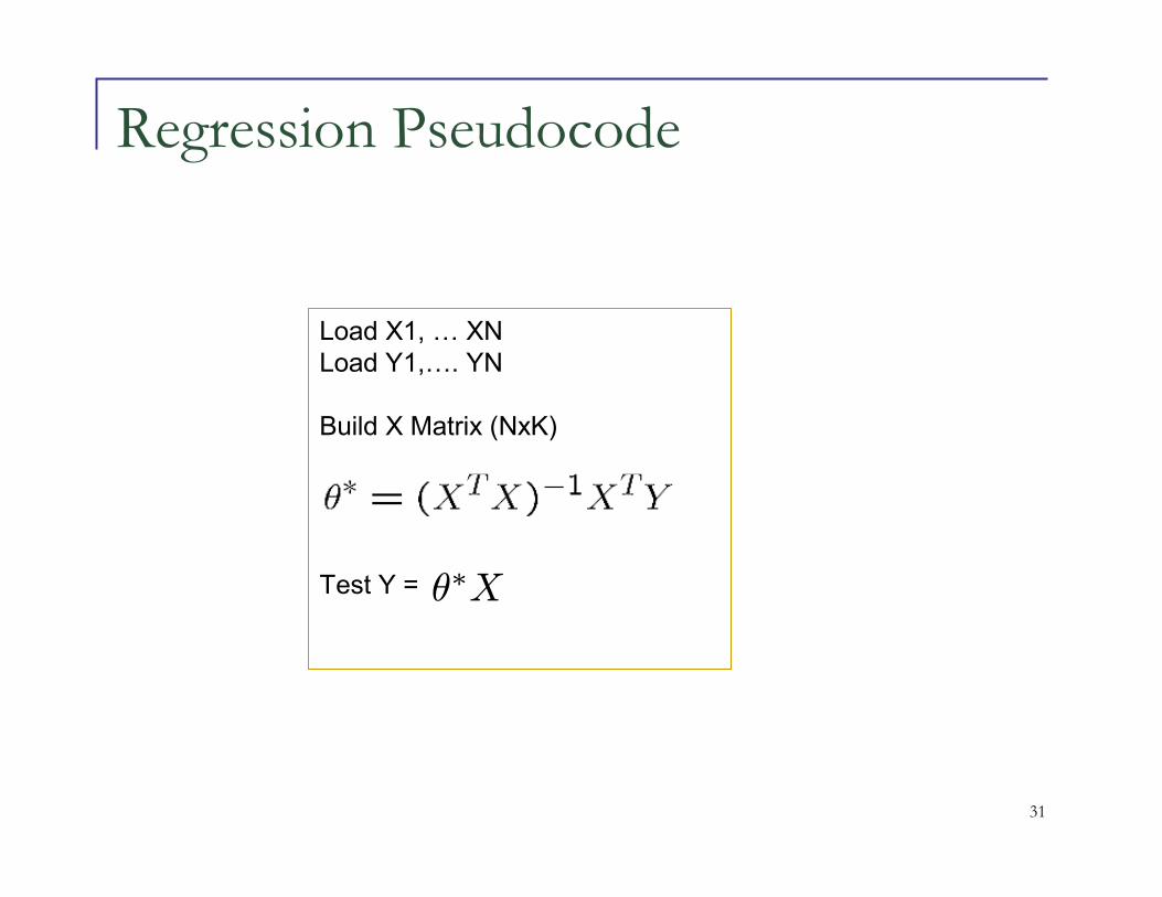
Regression Pseudocode
Load X1, … XNLoad Y1,…. YN
Build X Matrix (NxK)
Test Y = θ∗X
32
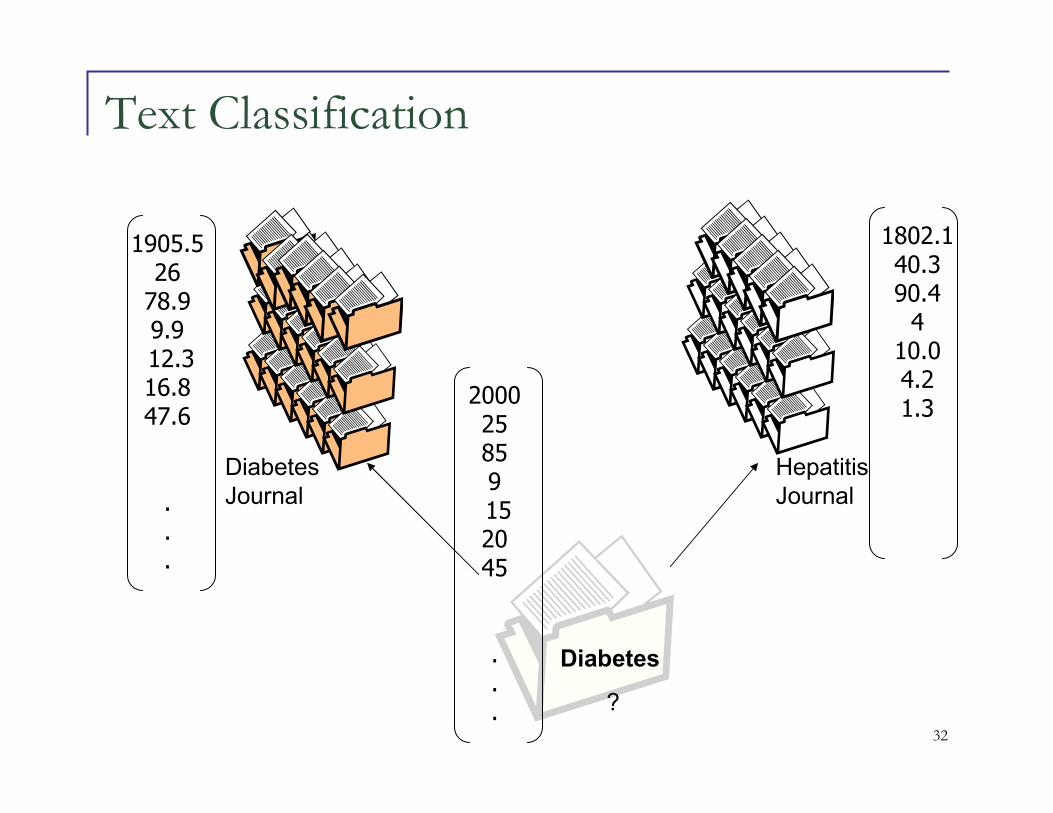
Text Classification
Diabetes
DiabetesJournal
HepatitisJournal
1802.140.390.44
10.04.21.3
1905.52678.99.912.316.847.6
.
.
.
200025859152045
.
.
. ?
33
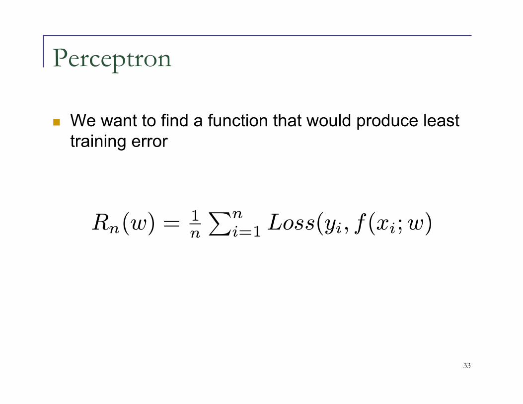
Perceptron
Rn(w) =1n
∑ni=1 Loss(yi, f(xi;w)
� We want to find a function that would produce least training error
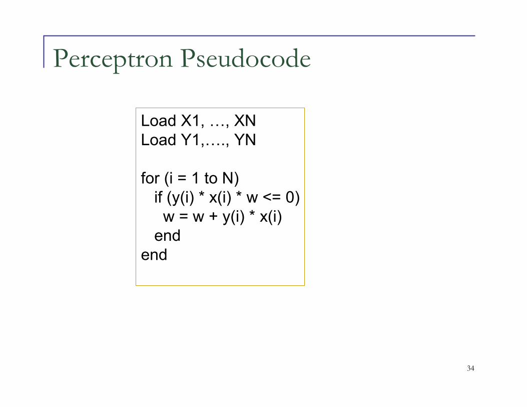
34
Perceptron Pseudocode
Load X1, …, XNLoad Y1,…., YN
for (i = 1 to N)if (y(i) * x(i) * w <= 0)w = w + y(i) * x(i)
endend

35
Naïve Bayes Classifier for Text
Prior Probability of the Class
Conditional Probability of feature given the Class
Here N is the number of words, not to confuse with the total vocabulary size
P (Yk,X1,X2, ..., XN ) = P (Yk)ΠiP (Xi|Yk)
36
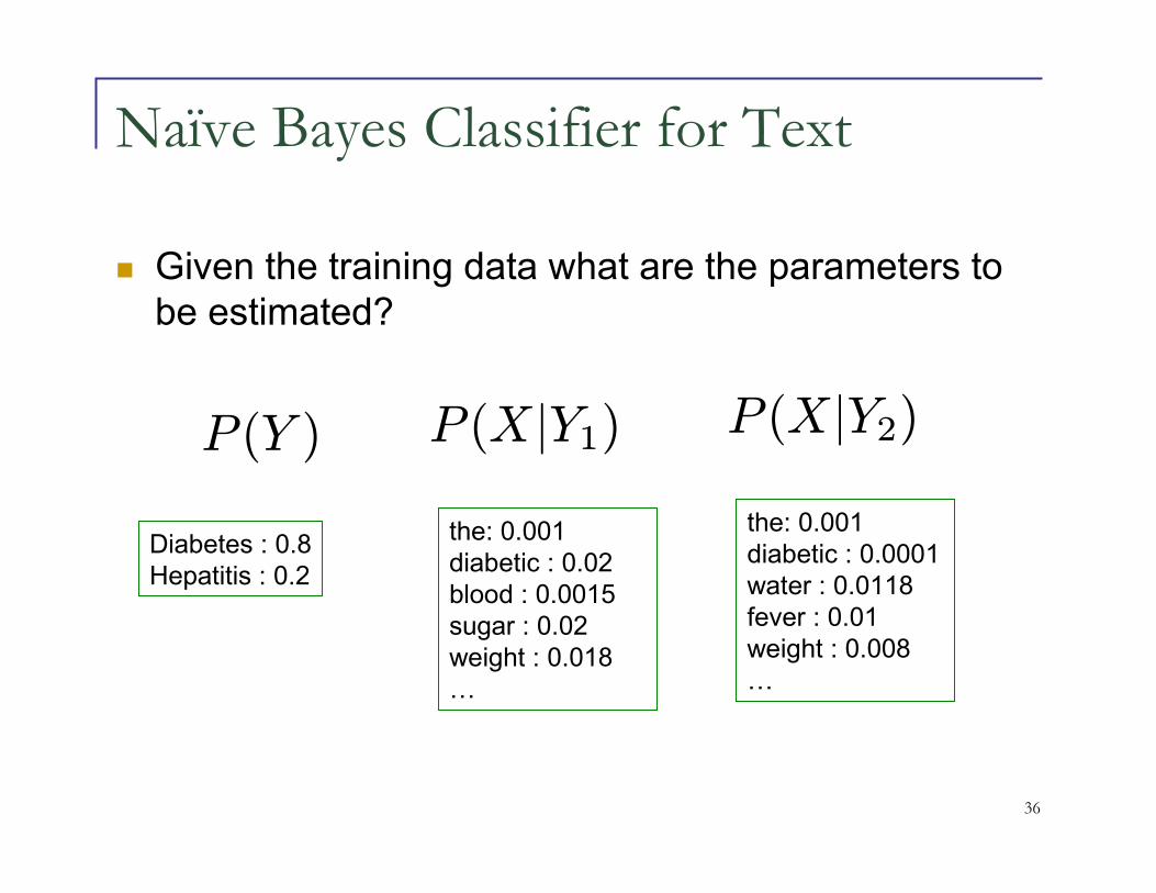
Naïve Bayes Classifier for Text
� Given the training data what are the parameters to be estimated?
P (X|Y2)P (X|Y1)P (Y )
Diabetes : 0.8Hepatitis : 0.2
the: 0.001diabetic : 0.02blood : 0.0015sugar : 0.02weight : 0.018…
the: 0.001diabetic : 0.0001water : 0.0118fever : 0.01weight : 0.008…

37
Naïve Bayes Pseudocode
Foreach Class CtotalWCount=0for J = 1 to |V| count(WJ)
endtotalCount = totalCount + totalCount(WJ)for J= 1 to |V|C.WJProb = count(WJ) + delta /totalCount(WJ) + delta * |V|
end end

38
SVM: Maximizing Margin with Constraints
� We can combine the two inequalities to get
� Problem formulation
� Minimize
� Subject to
‖w‖2
2
yi(wTxi + b)− 1 ≥ 0 ∀i
yi(wTxi + b)− 1 ≥ 0 ∀i
d+
d-

39
� Solve dual problem instead
� Maximize
� subject to constraints of
Dual Problem
J(α) =∑ni=1 αi −
12
∑ni,j=1 αiαjyiyj(xi.xj)
αi ≥ 0 ∀i
∑ni=1 αiyi = 0

40
SVM Solution
� Linear combination of weighted training example
� Sparse Solution, why?
� Weights zero for non-support vectors
∑i∈SV αiyi(xi.x) + b
w=∑ni=1 αiyixi
41
Sequential Minimal Optimization (SMO)
Algorithm
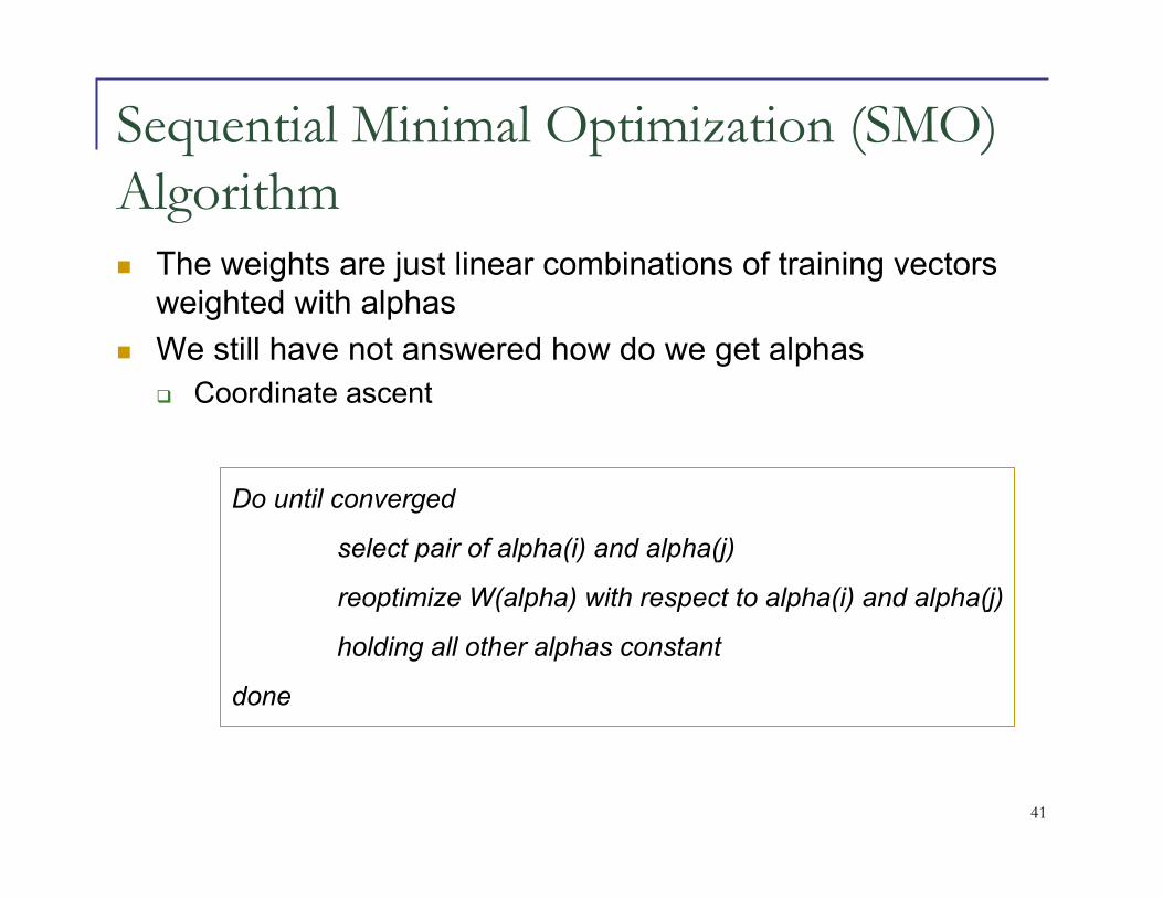
� The weights are just linear combinations of training vectors weighted with alphas
� We still have not answered how do we get alphas
� Coordinate ascent
Do until converged
select pair of alpha(i) and alpha(j)
reoptimize W(alpha) with respect to alpha(i) and alpha(j)
holding all other alphas constant
done

42
Information Extraction Tasks
� Named Entity Identification
� Relation Extraction
� Coreference resolution
� Term Extraction
� Lexical Disambiguation
� Event Detection and Classification
43
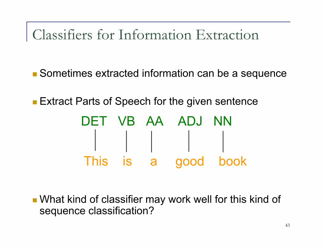
� Sometimes extracted information can be a sequence
� Extract Parts of Speech for the given sentence
� What kind of classifier may work well for this kind of sequence classification?
Classifiers for Information Extraction
DET VB AA ADJ NN
This is a good book
44
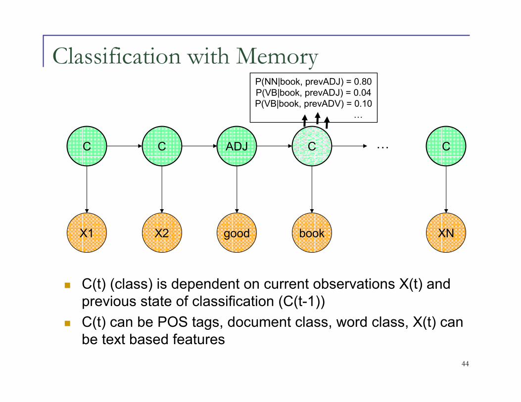
Classification with Memory
C
X1
C
X2
ADJ
good
C
book
C
XN
…
� C(t) (class) is dependent on current observations X(t) and previous state of classification (C(t-1))
� C(t) can be POS tags, document class, word class, X(t) can be text based features
P(NN|book, prevADJ) = 0.80P(VB|book, prevADJ) = 0.04P(VB|book, prevADV) = 0.10
…

45
HMM Example

46
Forward Algorithm : Computing alphas

47
Forward Algorithm Perl CodeSub Forward() {
for (my $t = 0; $t < @obs ; $t++){
#sum across i,j transitions for all starting i and ending at j
for (my $i = 0; $i < $num_states; $i++){
my $tot_forward_prob_for_cur_dest = 0;for (my $j = 0; $j < $num_states; $j++){
#multiply transition prob * obs probmy $trans_prob = $trans_matrix[$i][$j];
#get obs_idmy $cur_obs = $obs[$t];my $obs_id = $obs_vocab_id{$cur_obs};
#state i producing the given observationmy $obs_prob = $obs_matrix[$i][$obs_id];
#compute the forward probif ($t == 0){
my $start_trans_prob = $start_state_matrix[$j];$tot_forward_prob_for_cur_dest = $start_trans_prob * $obs_prob;
}else{
$tot_forward_prob_for_cur_dest = $tot_forward_prob_for_cur_dest + $forward_prob_matrix[$i][$t] * $trans_prob * $obs_prob;
}}#this is for passing on forward pass to next iteration
$forward_prob_matrix[$i][$t+1] = $tot_forward_prob_for_cur_dest;}
}}

48
Viterbi Algorithm

49
Problem 3: Forward-Backward
AlgorithmConsider transition from state i to j, trij
Let pt(trij,X) be the probability that trij is taken at time t, and the complete output is X.
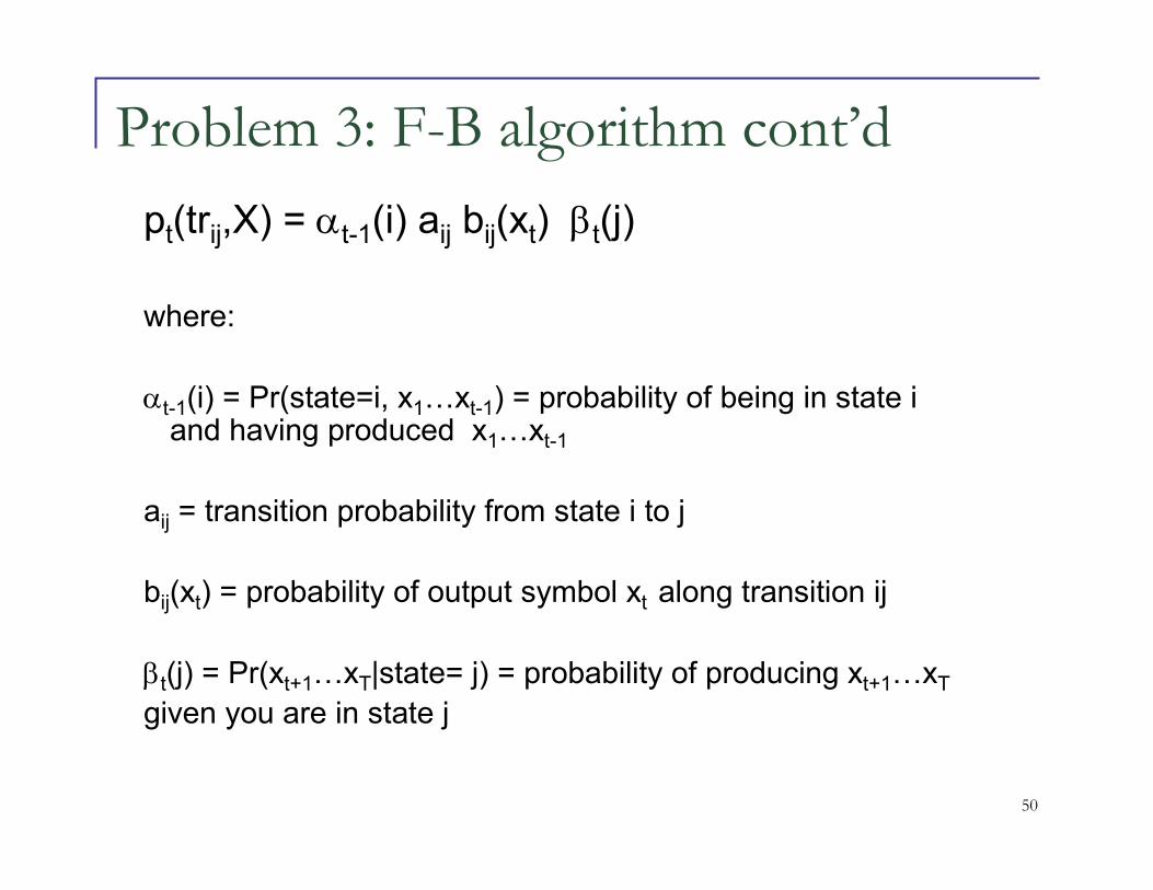
pt(trij,X) = αt-1(i) aij bij(xt) βt(j)
Si
Sj
αt-1(i) βt(j)
xt
50
Problem 3: F-B algorithm cont’d
pt(trij,X) = αt-1(i) aij bij(xt) βt(j)
where:
αt-1(i) = Pr(state=i, x1…xt-1) = probability of being in state i and having produced x1…xt-1
aij = transition probability from state i to j
bij(xt) = probability of output symbol xt along transition ij
βt(j) = Pr(xt+1…xT|state= j) = probability of producing xt+1…xT
given you are in state j

51
Estimating Transition and Emission
Probabilities
aijExpected number of transitions from state i to j
Expected number of transitions from state i=
bj (xt)Expected number of times in state j and observing symbol xt
Expected number of time in state j=
aij =count(i→j)∑q∈Q count(i→q)
52
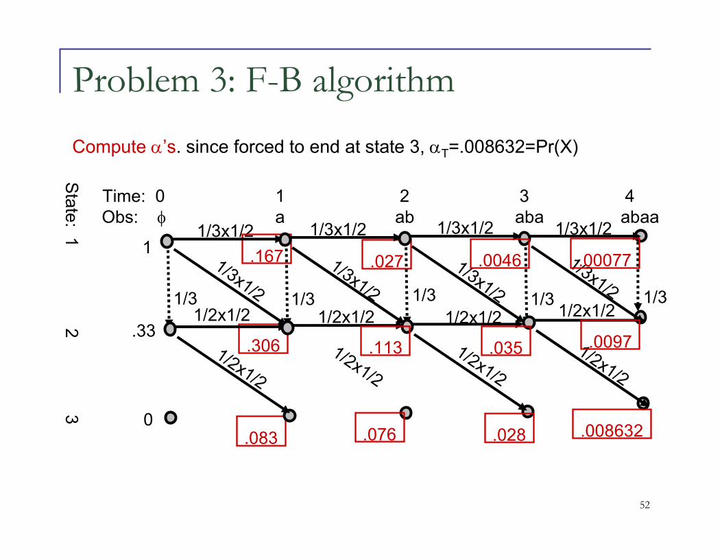
Problem 3: F-B algorithm
.083
Time: 0 1 2 3 4Obs: φ a ab aba abaa
Sta
te: 1
2 3
1/3x1/2 1/3x1/2 1/3x1/2 1/3x1/2
1/3 1/3 1/3 1/3 1/3
1/3x1/2
1/3x1/2
1/3x1/2
1/3x1/2
1/2x1/2 1/2x1/2 1/2x1/2 1/2x1/2
1/2x1/2
1/2x1/2
1/2x1/2
1/2x1/2
1
.33
0
.167
.306
.027
.076
Compute α’s. since forced to end at state 3, αT=.008632=Pr(X)
.113
.0046
.035
.028
.00077
.0097
.008632
Compute α’s. since forced to end at state 3, αT=.008632=Pr(X)

53
Problem 3: F-B algorithm, cont’d
0
Time: 0 1 2 3 4Obs: φ a ab aba abaa
Sta
te: 1
2 3
1/3x1/2 1/3x1/2 1/3x1/2 1/3x1/2
1/3 1/3 1/3 1/3 1/3
1/3x1/2
1/3x1/2
1/3x1/2
1/3x1/2
1/2x1/2 1/2x1/2 1/2x1/2 1/2x1/2
1/2x1/2
1/2x1/2
1/2x1/2
1/2x1/2
.0086
.0039
0
.028
.016
.076
0
Compute β’s.
.0625
.083
.25
0
0
0
1
54
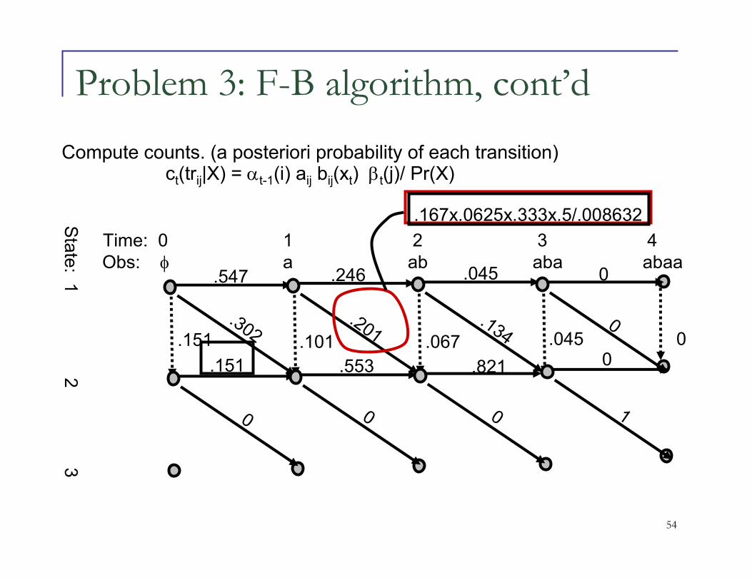
Problem 3: F-B algorithm, cont’d
Time: 0 1 2 3 4Obs: φ a ab aba abaa
Sta
te: 1
2 3
.547 .246 .045 0
.151 .101 .067 .045 0
.302.201
.1340
.151 .553 .821 0
00 0 1
Compute counts. (a posteriori probability of each transition)ct(trij|X) = αt-1(i) aij bij(xt) βt(j)/ Pr(X)
.167x.0625x.333x.5/.008632
55
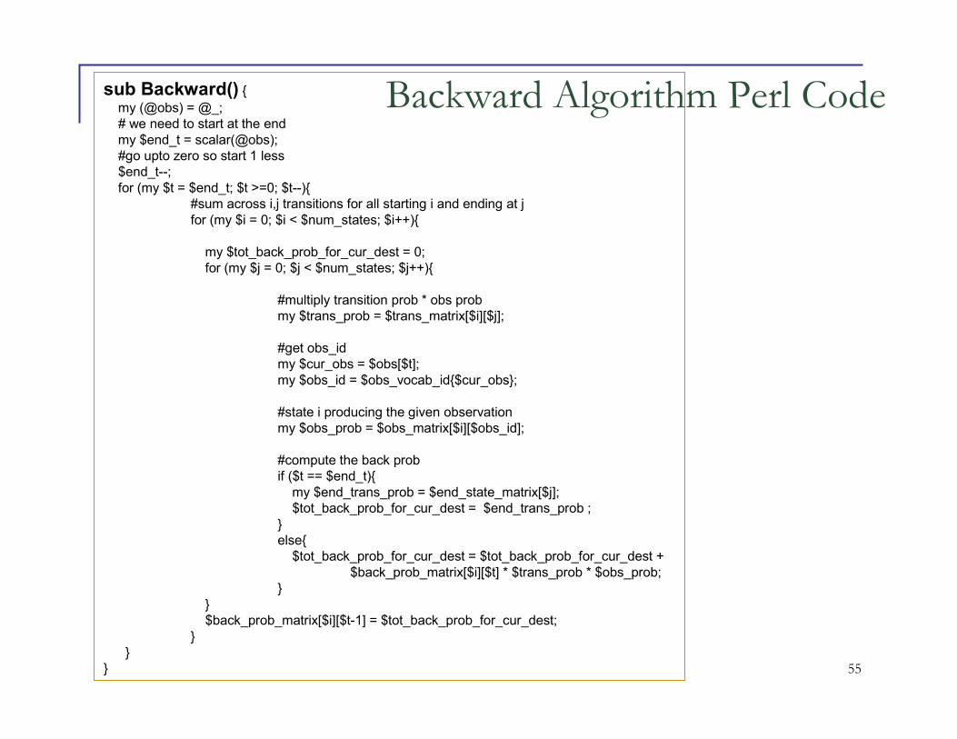
sub Backward() {
my (@obs) = @_;# we need to start at the endmy $end_t = scalar(@obs);#go upto zero so start 1 less$end_t--;for (my $t = $end_t; $t >=0; $t--){
#sum across i,j transitions for all starting i and ending at jfor (my $i = 0; $i < $num_states; $i++){
my $tot_back_prob_for_cur_dest = 0;for (my $j = 0; $j < $num_states; $j++){
#multiply transition prob * obs probmy $trans_prob = $trans_matrix[$i][$j];
#get obs_idmy $cur_obs = $obs[$t];my $obs_id = $obs_vocab_id{$cur_obs};
#state i producing the given observationmy $obs_prob = $obs_matrix[$i][$obs_id];
#compute the back probif ($t == $end_t){
my $end_trans_prob = $end_state_matrix[$j];$tot_back_prob_for_cur_dest = $end_trans_prob ;
}else{
$tot_back_prob_for_cur_dest = $tot_back_prob_for_cur_dest + $back_prob_matrix[$i][$t] * $trans_prob * $obs_prob;
}}$back_prob_matrix[$i][$t-1] = $tot_back_prob_for_cur_dest;
}}
}
Backward Algorithm Perl Code

56
Finding Maximum Likelihood of our Conditional
Models (Multinomial Logistic Regression)
P(C|D,λ) =∑
(c,d)∈(C,D)
logexp
∑i λifi(c,d)∑
c′ exp∑i λifi(c
′, d)
P(C|D,λ) =∑
(c,d)∈(C,D)
logp(c|d,λ)
(C|D,λ) =∏
(c,d)∈(C,D)
p(c|d,λ)
57
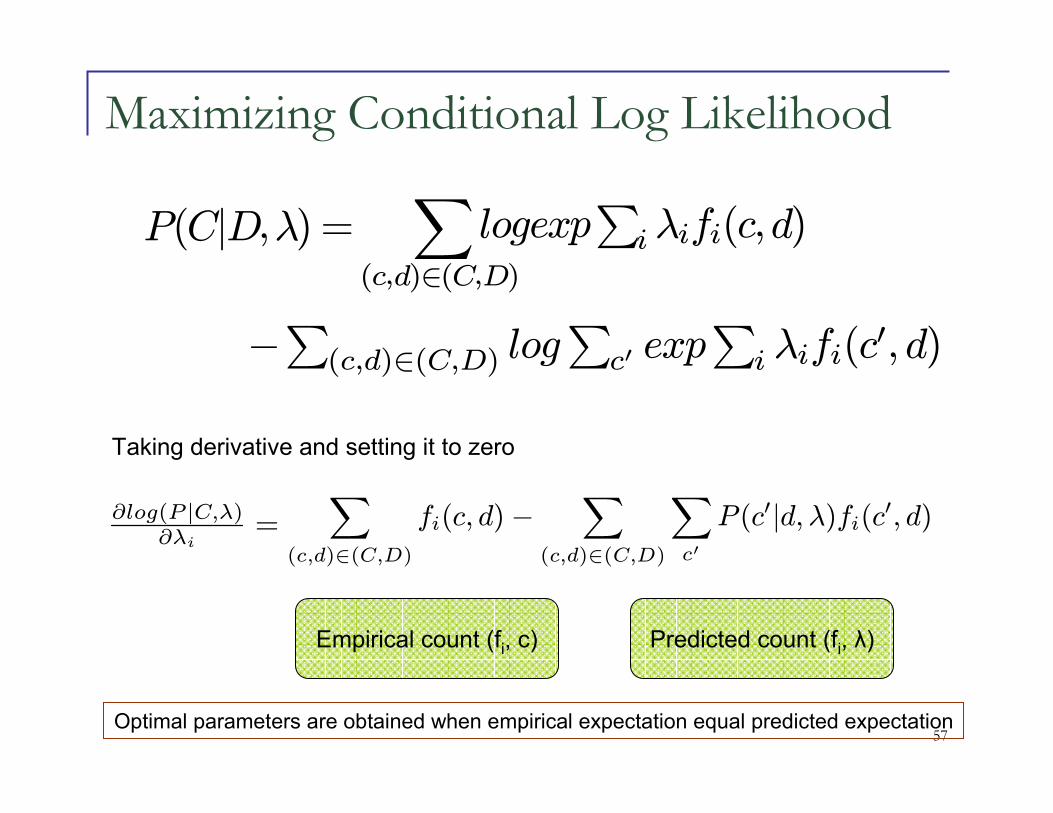
Maximizing Conditional Log Likelihood
P(C|D,λ) =∑
(c,d)∈(C,D)
−∑(c,d)∈(C,D) log
∑c′ exp
∑i λifi(c
′, d)
logexp∑iλifi(c,d)
∑
(c,d)∈(C,D)
fi(c, d)−∑
(c,d)∈(C,D)
∑
c′
P (c′|d, λ)fi(c′, d)∂log(P |C,λ)
∂λi=
Empirical count (fi, c) Predicted count (fi, λ)
Optimal parameters are obtained when empirical expectation equal predicted expectation
Taking derivative and setting it to zero

58
Finding Model Parameters
� We saw that optimum parameters are obtained when empirical expectation of a feature equals predicted expectation
� We are finding a model having maximum entropy and satisfying constraints for all features fj
� Hence finding the parameters of maximum entropy model entails to maximizing conditional log-likelihood and solving it� Conjugate Gradient Descent� Quasi Newton’s Method
� A simple iterative scaling� Features are non-negative (indicator functions are non-negative)� Add a slack feature
� where
Ep(fj) = E(p)(fj)
M = maxi,c∑mj=1 fj(di, c)
fm+1(d, c) =M −∑mj=1 fj(d, c)

59
Finding Model Parameters� We saw that optimum parameters are obtained when empirical
expectation of a feature equals predicted expectation� We are finding a model having maximum entropy and satisfying
constraints for all features fj
� Hence finding the parameters of maximum entropy model entails tomaximizing conditional log-likelihood and solving it� Conjugate Gradient Descent� Quasi Newton’s Method� A simple iterative scaling
� Features are non-negative (indicator functions are non-negative)� Add a slack feature
� where
Ep(fj) = E(p)(fj)
M = maxi,c∑mj=1 fj(di, c)
fm+1(d, c) =M −∑mj=1 fj(d, c)
60
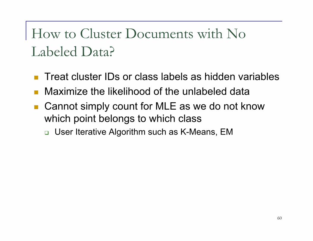
How to Cluster Documents with No
Labeled Data?
� Treat cluster IDs or class labels as hidden variables
� Maximize the likelihood of the unlabeled data
� Cannot simply count for MLE as we do not know which point belongs to which class
� User Iterative Algorithm such as K-Means, EM
61
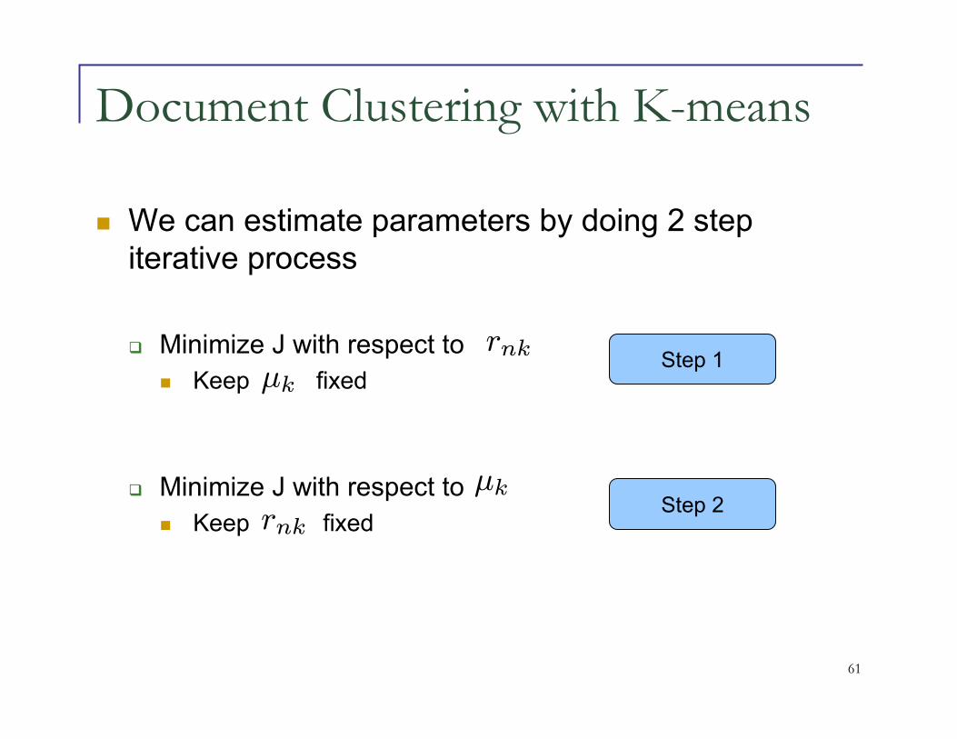
Document Clustering with K-means
� We can estimate parameters by doing 2 step iterative process
� Minimize J with respect to
� Keep fixed
� Minimize J with respect to
� Keep fixed
rnkµk
µkrnk
Step 1
Step 2

62
� Optimize for each n separately by choosing for k that gives minimum
� Assign each data point to the cluster that is the closest
� Hard decision to cluster assignment
rnk
||xn − rnk||2
rnk = 1 if k = argminj ||xn − µj ||2
= 0 otherwise
rnkµk
Step 1� Minimize J with respect to
� Keep fixed

63
� J is quadratic in . Minimize by setting derivative w.rt. to zero
� Take all the points assigned to cluster K and re-estimate the mean for cluster K
� Minimize J with respect to
� Keep fixedrnk
µkStep 2
µk µk
µk =
∑n rnkxn∑n rnk

64
Expectation Maximization for Gaussian
Mixture Models
� E-Step
γ(znk) = E(znk|xn) = p(zk = 1|xn)
γ(znk) =πkN (xn|µk,
∑k)
∑Kj=1 πjN (xn|µj ,
∑j)

65
Estimating Parameters
� M-step
� Iterate until convergence of log likelihood
π′k =Nk
N
log p(X|π, µ,∑) =
∑Nn=1 log (
∑kk=1N (x|µk,
∑k))
µ′k =1Nk
∑Nn=1 γ(znk)xn
∑′k =
1Nk
∑Nn=1 γ(znk)(xn − µ
′k)(xn − µ
′k)T
where Nk =∑Nn=1 γ(znk)

66
Maximum Entropy Markov Model
T = argmaxTP (W |T )P (T )
T = argmaxTP (T |W )
T = argmaxTP (T |W )
MEMM Inference
HMM Inference
= argmaxT∏i P (ti|ti−1, wi)
= argmaxT∏i P (wi|ti)p(ti|ti−1)
67
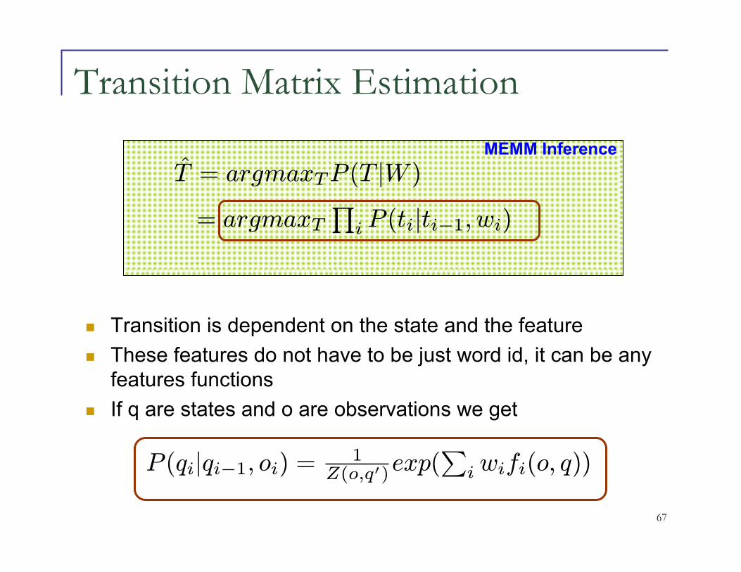
Transition Matrix Estimation
P (qi|qi−1, oi) =1
Z(o,q′)exp(∑i wifi(o, q))
T = argmaxTP (T |W )MEMM Inference
= argmaxT∏i P (ti|ti−1, wi)
� Transition is dependent on the state and the feature
� These features do not have to be just word id, it can be any features functions
� If q are states and o are observations we get

68
Viterbi in HMM vs. MEMM
� HMM decoding:
� MEMM decoding:
This computed in maximum entropy frameworkbut has markov assumption in states thus its name MEMM
vt(j) = maxNi=1vt−1(i)P (sj |si)P (ot|sj) 1 ≤ j ≤ N, 1 < t ≤ T
vt(j) = maxNi=1vt−1(i)P (sj |si, ot) 1 ≤ j ≤ N, 1 < t ≤ T

69
Conditional Random Field
FeatureFunctions
Weight forgiven feature function
Feature function can access all of observation
Sum overall data points
Sum overall feature function
Sum overall possible label sequence
Model log linear on Feature functions
P (y|x;w) =
exp(
∑
i
∑
j
wjfj(yi−1, yi, x, i))
∑
y′∈Y
exp(∑
i
∑
j
wjfj(y′i−1, y
′i, x, i))

70
Inference in Linear Chain CRF
� We saw how to do inference in HMM and MEMM
� We can still do Viterbi dynamic programming based inference
y∗ = argmaxyp(y|x;w)
= argmaxy∑j wjFj(x, y)
= argmaxy∑i gi(yi−1, yi)
wheregi(yi−1, yi) =∑j wjfj(yi−1, yi, x, i)
= argmaxy∑j wj
∑i fj(yi−1, yi, x, i)
x and i arguments of f_j dropped in definition of g_ig_i is different for each I, depends on w, x and i
Denominator?

71
Computing Expected Counts
Need to compute denominator
P (y|x;w) =
exp(
∑
i
∑
j
wjfj(yi−1, yi, x, i))
∑
y′∈Y
exp(∑
i
∑
j
wjfj(y′i−1, y
′i, x, i))
72
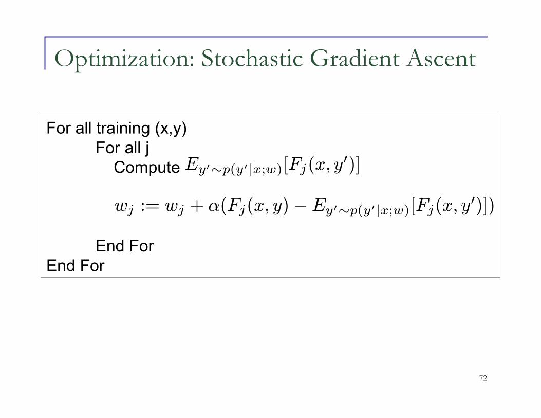
Optimization: Stochastic Gradient Ascent
For all training (x,y)For all j
Compute
End ForEnd For
Ey′∼p(y′|x;w)[Fj(x, y′)]
wj := wj + α(Fj(x, y)−Ey′∼p(y′|x;w)[Fj(x, y′)])

73
References
� [1] Christopher Bishop, “Pattern Recognition and Machine Learning” 2006
� [2] David Smith and Jason Eisner, “Dependency Parsing by Belief Propagation,” Proceedings of the 2008 Conference on Empirical Methods in Natural Language Processing, pages 145–156, Honolulu, October 2008.