statistical testing in nlp (ii)

Statistical Testing in NLP (II)

CS 690N, Spring 2018Advanced Natural Language Processing

http://people.cs.umass.edu/~brenocon/anlp2018/

Brendan O’ConnorCollege of Information and Computer Sciences

University of Massachusetts Amherst

Tuesday, February 27, 18



Statistical variability in NLP

• How to trust experiment results, given many sources of variability?

• How was the text data sampled?

• How were the annotations sampled?

• How variably do the human annotators behave?

• How variable are the computational algorithms?

• Today: Variability due to small sample size

2


Text data variability

• Mathematically, the easiest case to analyze:What if we resampled the tokens/sentences/documents from a similar population as our current data sample?

• Assume units are sampled i.i.d.; then apply your favorite statistical significance/confidence interval testing technique

• T-tests, binomial tests, ...

• Bootstrapping

• Paired tests

• For

• 1. Null hypothesis testing

• 2. Confidence intervals

3


Null hypothesis test

• Must define a null hypothesis you wish to ~disprove

• pvalue = Probability of a result as least as extreme, if the null hypothesis was active

• Example: paired testing of classifiers with exact binomial test (R: binom.test)

4

3.4. EVALUATING CLASSIFIERS 77

Figure 3.5: Probability mass function for the binomial distribution. The pink highlightedareas represent the cumulative probability for a significance test on an observation ofk = 10 and N = 30.

We write k ⇠ Binom(✓, N) to indicate that k is drawn from a binomial distribution, withparameter N indicating the number of random “draws”, and ✓ indicating the probabilityof “success” on each draw. The probability mass function (PMF) of the binomial distri-bution is,

pBinom(k; N, ✓) =

✓N

k

◆✓k(1 � ✓)N�k, [3.9]

with ✓k representing the probability of the k successes, (1 � ✓)N�k representing the prob-ability of the N � k unsuccessful draws. The expression

�Nk

�= N !

k!(N�k)! is a binomialcoefficient, representing the number of possible orderings of events; this ensures that thedistribution sums to one over all k 2 {0, 1, 2, . . . , N}.

Under the null hypothesis, ✓ = 1

2

: when the classifiers disagree, they are each equallylikely to be right. Now suppose that among N disagreements, c

1

is correct only k <N2

times. The probability of c1

being correct k or fewer times is the one-tailed p-value,because it is computed from the area under the binomial probability mass function from0 to k, as shown in the left tail of Figure 3.5. This cumulative probability is computed asa sum over all values i k,

PrBinom

✓count(y(i)

2

= y(i) 6= y(i)1

) k; N, ✓ =1

2

◆=

kXi=0

pBinom

✓i; N, ✓ =

1

2

◆. [3.10]

The one-tailed p-value applies only to the asymmetric null hypothesis that c1

is at leastas accurate as c

2

. To test the two-tailed null hypothesis that c1

and c2

are equally accu-rate, we would take the sum of one-tailed p-values, where the second term is computedfrom the right tail of Figure 3.5. The binomial distribution is symmetric, so this can becomputed by simply doubling the one-tailed p-value.

(c) Jacob Eisenstein 2018. Work in progress.

3.4. EVALUATING CLASSIFIERS 77

Figure 3.5: Probability mass function for the binomial distribution. The pink highlightedareas represent the cumulative probability for a significance test on an observation ofk = 10 and N = 30.

We write k ⇠ Binom(✓, N) to indicate that k is drawn from a binomial distribution, withparameter N indicating the number of random “draws”, and ✓ indicating the probabilityof “success” on each draw. The probability mass function (PMF) of the binomial distri-bution is,

pBinom(k; N, ✓) =

✓N

k

◆✓k(1 � ✓)N�k, [3.9]

with ✓k representing the probability of the k successes, (1 � ✓)N�k representing the prob-ability of the N � k unsuccessful draws. The expression

�Nk

�= N !

k!(N�k)! is a binomialcoefficient, representing the number of possible orderings of events; this ensures that thedistribution sums to one over all k 2 {0, 1, 2, . . . , N}.

Under the null hypothesis, ✓ = 1

2

: when the classifiers disagree, they are each equallylikely to be right. Now suppose that among N disagreements, c

1

is correct only k <N2

times. The probability of c1

being correct k or fewer times is the one-tailed p-value,because it is computed from the area under the binomial probability mass function from0 to k, as shown in the left tail of Figure 3.5. This cumulative probability is computed asa sum over all values i k,

PrBinom

✓count(y(i)

2

= y(i) 6= y(i)1

) k; N, ✓ =1

2

◆=

kXi=0

pBinom

✓i; N, ✓ =

1

2

◆. [3.10]

The one-tailed p-value applies only to the asymmetric null hypothesis that c1

is at leastas accurate as c

2

. To test the two-tailed null hypothesis that c1

and c2

are equally accu-rate, we would take the sum of one-tailed p-values, where the second term is computedfrom the right tail of Figure 3.5. The binomial distribution is symmetric, so this can becomputed by simply doubling the one-tailed p-value.

(c) Jacob Eisenstein 2018. Work in progress.


Statistical tests

• Closed-form tests

• t-tests, exact binomial test, chi-square tests....

• Bootstrapping

• All methods can give both p-values and confidence intervals

5


Bootstrapping• Bootstrapped CI methods

• Percentile

• Standard error-based normal approx, etc.

• Theoretical guarantees (under various regularity conditions... for

a slightly different CI method...):

6

Bootstrap Confidence Interval

1. Draw a bootstrap sample X⇤1

, . . . , X⇤n ⇠ Pn. Compute b✓⇤n = g(X⇤

1

, . . . , X⇤n).

2. Repeat the previous step, B times, yielding estimators b✓⇤n,1, . . . , b✓⇤n,B.

3. Let

bF (t) =1

B

BX

j=1

I⇣p

n(b✓⇤n,j � b✓n⌘ t).

4. Let

Cn =

b✓n �

t1�↵/2p

n, b✓n �

t↵/2pn

�

where t↵/2 = bF�1(↵/2) and t1�↵/2 = bF�1(1� ↵/2).

5. Output Cn.

Theorem 2 Under appropriate regularity conditions,

P(✓ 2 Cn) = 1� ↵�O

✓1pn

◆.

as n ! 1.

See the appendix for a discussion of the regularity conditions.

4 Examples

Example 3 Consider the polynomial regression model Y = g(X) + ✏ where X, Y 2 R andg(x) = �

0

+ �1

x + �2

x2. Given data (X1

, Y1

), . . . , (Xn, Yn) we can estimate � = (�0

, �1

, �2

)with the least squares estimator b�. Suppose that g(x) is concave and we are interested inthe location at which g(x) is maximized. It is easy to see that the maximum occurs at x = ✓

where ✓ = �(1/2)�1

/�2

. A point estimate of ✓ is b✓ = �(1/2)b�1

/b�2

. Now we use thebootstrap to get a confidence interval for ✓. Figure 1 shows 50 points drawn from the abovemodel with �

0

= �1, �1

= 2, �2

= �1. The Xi’s were sample uniformly on [0, 2] and wetook ✏i ⇠ N(0, .22). In this case, ✓ = 1. The true and estimated curves are shown in thefigure. At the bottom of the plot we show the 95 percent boostrap confidence interval basedon B = 1, 000.

4

• How many samples? 10,000-100,000(governs monte carlo error; can always make nearly 0)

• Paired bootstrap

• Bootstrapped p-values


• (stopped here 2/27)

7


Berg-Kirkpatrick et al. 2012

• Paired bootstrap test

• (Subtle, debatable bug?)

• Stat. sig results may not transfer domains

• Researcher effects? Or is paired testing working correctly?

8


9

As mentioned, a major benefit of the bootstrap isthat any evaluation metric can be used to compute�(x).3 We run the bootstrap using several metrics:F1-measure for constituency parsing, unlabeled de-pendency accuracy for dependency parsing, align-ment error rate (AER) for word alignment, ROUGEscore (Lin, 2004) for summarization, and BLEUscore for machine translation.4 We report all met-rics as percentages.

3 Experiments

Our first goal is to explore the relationship be-tween metric gain, �(x), and statistical significance,p-value(x), for a range of NLP tasks. In order to sayanything meaningful, we will need to see both �(x)and p-value(x) for many pairs of systems.

3.1 Natural Comparisons

Ideally, for a given task and test set we could obtainoutputs from all systems that have been evaluatedin published work. For each pair of these systemswe could run a comparison and compute both �(x)and p-value(x). While obtaining such data is notgenerally feasible, for several tasks there are pub-lic competitions to which systems are submitted bymany researchers. Some of these competitions makesystem outputs publicly available. We obtained sys-tem outputs from the TAC 2008 workshop on auto-matic summarization (Dang and Owczarzak, 2008),the CoNLL 2007 shared task on dependency parsing(Nivre et al., 2007), and the WMT 2010 workshopon machine translation (Callison-Burch et al., 2010).

For cases where the metric linearly decomposes over sentences,the mean of �(x(i)) is �(x). By the central limit theorem, thedistribution will be symmetric for large test sets; for small testsets it may not.

3Note that the bootstrap procedure given only approximatesthe true significance level, with multiple sources of approxima-tion error. One is the error introduced from using a finite num-ber of bootstrap samples. Another comes from the assumptionthat the bootstrap samples reflect the underlying population dis-tribution. A third is the assumption that the mean bootstrap gainis the test gain (which could be further corrected for if the metricis sufficiently ill-behaved).

4To save time, we can compute �(x) for each bootstrap sam-ple without having to rerun the evaluation metric. For our met-rics, sufficient statistics can be recorded for each sentence andthen sampled along with the sentences when constructing eachx

(i) (e.g. size of gold, size of guess, and number correct are suf-ficient for F1). This makes the bootstrap very fast in practice.

0.5

0.6

0.7

0.8

0.9

1

0 0.5 1 1.5 2

1 -

p-v

alue

ROUGE

Different research groupsSame research group

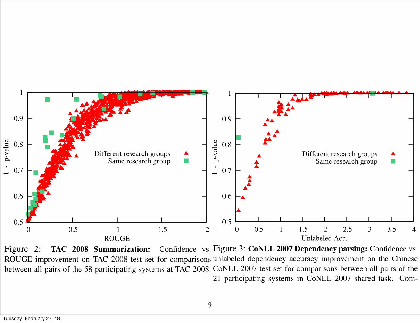
Figure 2: TAC 2008 Summarization: Confidence vs.ROUGE improvement on TAC 2008 test set for comparisonsbetween all pairs of the 58 participating systems at TAC 2008.Comparisons between systems entered by the same researchgroup and comparisons between systems entered by differentresearch groups are shown separately.

3.1.1 TAC 2008 SummarizationIn our first experiment, we use the outputs of the

58 systems that participated in the TAC 2008 work-shop on automatic summarization. For each possi-ble pairing, we compute �(x) and p-value(x) on thenon-update portion of the TAC 2008 test set (we or-der each pair so that the gain, �(x), is always pos-itive).5 For this task, test instances correspond todocument collections. The test set consists of 48document collections, each with a human producedsummary. Figure 2 plots the ROUGE gain against1 � p-value, which we refer to as confidence. Eachpoint on the graph corresponds to an individual pairof systems.

As expected, larger gains in ROUGE correspondto higher confidences. The curved shape of the plotis interesting. It suggests that relatively quickly wereach ROUGE gains for which, in practice, signif-icance tests will most likely be positive. We mightexpect that systems whose outputs are highly corre-lated will achieve higher confidence at lower met-ric gains. To test this hypothesis, in Figure 2 we

5In order to run bootstraps between all pairs of systemsquickly, we reuse a random sample counts matrix between boot-strap runs. As a result, we no longer need to perform quadrat-ically many corpus resamplings. The speed-up from this ap-proach is enormous, but one undesirable effect is that the boot-strap estimation noise between different runs is correlated. As aremedy, we set b so large that the correlated noise is not visiblein plots.

0.5

0.6

0.7

0.8

0.9

1

0 0.5 1 1.5 2 2.5 3 3.5 4

1

- p

-val

ue

Unlabeled Acc.

Different research groupsSame research group

Figure 3: CoNLL 2007 Dependency parsing: Confidence vs.unlabeled dependency accuracy improvement on the ChineseCoNLL 2007 test set for comparisons between all pairs of the21 participating systems in CoNLL 2007 shared task. Com-parisons between systems entered by the same research groupand comparisons between systems entered by different researchgroups are shown separately.

separately show the comparisons between systemsentered by the same research group and compar-isons between systems entered by different researchgroups, with the expectation that systems entered bythe same group are likely to have more correlatedoutputs. Many of the comparisons between systemssubmitted by the same group are offset from themain curve. It appears that they do achieve higherconfidences at lower metric gains.

Given the huge number of system comparisons inFigure 2, one obvious question to ask is whetherwe can take the results of all these statistical sig-nificance tests and estimate a ROUGE improvementthreshold that predicts when future statistical sig-nificance tests will probably be significant at thep-value(x) < 0.05 level. For example, let’s say wetake all the comparisons with p-value between 0.04and 0.06 (47 comparisons in all in this case). Eachof these comparisons has an associated metric gain,and by taking, say, the 95th percentile of these met-ric gains, we get a potentially useful threshold. Inthis case, the computed threshold is 1.10 ROUGE.

What does this threshold mean? Well, based onthe way we computed it, it suggests that if somebodyreports a ROUGE increase of around 1.10 on the ex-act same test set, there is a pretty good chance that astatistical significance test would show significanceat the p-value(x) < 0.05 level. After all, 95% of

the borderline significant differences that we’ve al-ready seen showed an increase of even less than 1.10ROUGE. If we’re evaluating past work, or are insome other setting where system outputs just aren’tavailable, the threshold could guide our interpreta-tion of reports containing only summary scores.

That being said, it is important that we don’t over-interpret the meaning of the 1.10 ROUGE threshold.We have already seen that pairs of systems submit-ted by the same research group and by different re-search groups follow different trends, and we willsoon see more evidence demonstrating the impor-tance of system correlation in determining the rela-tionship between metric gain and confidence. Addi-tionally, in Section 4, we will see that properties ofthe test corpus have a large effect on the trend. Thereare many factors are at work, and so, of course, met-ric gain alone will not fully determine the outcomeof a paired significance test.

3.1.2 CoNLL 2007 Dependency ParsingNext, we run an experiment for dependency pars-

ing. We use the outputs of the 21 systems that par-ticipated in the CoNLL 2007 shared task on depen-dency parsing. In Figure 3, we plot, for all pairs,the gain in unlabeled dependency accuracy againstconfidence on the CoNLL 2007 Chinese test set,which consists of 690 sentences and parses. Weagain separate comparisons between systems sub-mitted by the same research group and those submit-ted by different groups, although for this task therewere fewer cases of multiple submission. The re-sults resemble the plot for summarization; we againsee a curve-shaped trend, and comparisons betweensystems from the same group (few that they are)achieve higher confidences at lower metric gains.

3.1.3 WMT 2010 Machine TranslationOur final task for which system outputs are pub-

licly available is machine translation. We run an ex-periment using the outputs of the 31 systems par-ticipating in WMT 2010 on the system combinationportion of the German-English WMT 2010 news testset, which consists of 2,034 German sentences andEnglish translations. We again run comparisons forpairs of participating systems. We plot gain in testBLEU score against confidence in Figure 4. In thisexperiment there is an additional class of compar-


10

4.2 Empirical Calibration across Domains

Now that we have a way of generating outputs forthousands of pairs of systems, we can check empir-ically the practical reliability of significance testing.Recall that the bootstrap p-value(x) is an approxi-mation to p(�(X) > �(x)|H0). However, we oftenreally want to determine the probability that the newsystem is better than the baseline on the underlyingtest distribution or even the distribution from anotherdomain. There is no reason a priori to expect thesenumbers to coincide.

In our next experiment, we treat the entire Browncorpus, which consists of 24K sentences, as the truepopulation of English sentences. For each systemgenerated in the way described in Section 3.2.5 wecompute F1 on all of Brown. Since we are treat-ing the Brown corpus as the actual population of En-glish sentences, for each pair of parsers we can saythat the sign of the F1 difference indicates which isthe truly better system. Now, we repeatedly resam-ple small test sets from Brown, each consisting of1,600 sentences, drawn by sampling sentences withreplacement. For each pair of systems, and for eachresampled test set, we compute p-value(x) using thebootstrap. Out of the 4K bootstraps computed in thisway, 942 had p-value between 0.04 and 0.06, 869of which agreed with the sign of the F1 differencewe saw on the entire Brown corpus. Thus, 92% ofthe significance tests with p-value in a tight rangearound 0.05 correctly identified the better system.

This result is encouraging. It suggests that sta-tistical significance computed using the bootstrap isreasonably well calibrated. However, test sets arealmost never drawn i.i.d. from the distribution of in-stances the system will encounter in practical use.Thus, we also wish to compute how calibration de-grades as the domain of the test set changes. In an-other experiment, we look at how significance nearp-value = 0.05 on section 23 of the WSJ corpuspredicts performance on sections 22 and 24 and theBrown corpus. This time, for each pair of generatedsystems we run a bootstrap on section 23. Out ofall these bootstraps, 58 system pairs had p-value be-tween 0.04 and 0.06. Of these, only 83% had thesame sign of F1 difference on section 23 as they didon section 22, 71% the had the same sign on sec-tion 23 as on section 24, and 48% the same sign on

Sec. 23 p-value % Sys. A > Sys. BSec. 22 Sec. 24 Brown

0.00125 - 0.0025 97% 95% 73%0.0025 - 0.005 92% 92% 60%0.005 - 0.01 92% 85% 56%0.01 - 0.02 88% 92% 54%0.02 - 0.04 87% 78% 51%0.04 - 0.08 83% 74% 48%

Table 1: Empirical calibration: p-value on section 23 of theWSJ corpus vs. fraction of comparisons where system A beatssystem B on section 22, section 24, and the Brown corpus. Notethat system pairs are ordered so that A always outperforms B onsection 23.

section 23 as on the Brown corpus. This indicatesthat reliability degrades as we switch the domain. Inthe extreme, achieving a p-value near 0.05 on sec-tion 23 provides no information about performanceon the Brown corpus.

If we intend to use our system on out-of-domaindata, these results are somewhat discouraging. Howlow does p-value(x) have to get before we start get-ting good information about out-of-domain perfor-mance? We try to answer this question for this par-ticular parsing task by running the same domain cal-ibration experiment for several different ranges ofp-value. The results are shown in Table 1. Fromthese results, it appears that for constituency pars-ing, when testing on section 23, a p-value level be-low 0.00125 is required to reasonably predict perfor-mance on the Brown corpus.

It should be considered a good practice to includestatistical significance testing results with empiri-cal evaluations. The bootstrap in particular is easyto run and makes relatively few assumptions aboutthe task or evaluation metric. However, we havedemonstrated some limitations of statistical signifi-cance testing for NLP. In particular, while statisticalsignificance is usually a minimum necessary condi-tion to demonstrate that a performance difference isreal, it’s also important to consider the relationshipbetween test set performance and the actual goalsof the systems being tested, especially if the systemwill eventually be used on data from a different do-main than the test set used for evaluation.

5 ConclusionWe have demonstrated trends relating several im-portant factors to significance level, which include


• Statistical significance != practical significance

• CI width, statistical power, data size

• Many other confounds we don’t have models for, but know can be very significant

• Researcher bias

• File-drawer bias

• Generalization (e.g. across domains)

• Tuning on test sets

• Reusing test set over multiple papers

11


statistical testing in nlp (ii)

Documents